qutip: quantum toolbox in python - amazon...

DTU, Copenhagen, 2014 [email protected] 1

Introduction to

QuTiP: Quantum Toolbox in Python

with circuit-QED applications

Robert JohanssonRIKEN

In collaboration with

Paul NationKorea University

Franco NoriRIKEN / Michigan University


Content

● Introduction to QuTiP

● Example notebooks

– Getting started with QuTiP

– Jaynes-Cumming-like models

● Vacuum Rabi oscillations

● Single-atom laser

– Spectrum of dispersively coupled atom-cavity system


2000 2005 2010

NEC 1999

qubits

qubit-qubit

qubit-resonator

resonator as coupling bus

high level of controlof resonators

Delft 2003

NIST 2007

NEC 2007

NIST 2002

Saclay 2002

Saclay 1998 Yale 2008

Yale 2011

UCSB 2012

UCSB 2006

NEC 2003

Yale 2004

UCSB 2009

UCSB 2009

ETH 2008

ETH 2010

Chalmers 2008


What is QuTiP?

● Framework for computational quantum dynamics

– Efficient and easy to use for quantum physicists

– Thoroughly tested (100+ unit tests)

– Well documented (200+ pages, 50+ examples)

– Quite large number of users (>1000 downloads)

● Suitable for

– theoretical modeling and simulations

– modeling experiments

● 100% open source

● Implemented in Python/Cython using SciPy, Numpy, and matplotlib


Project information

Authors: Robert Johansson and Paul Nation

Web site: http://www.qutip.org

Discussion: Google group “qutip”

Blog: http://qutip.blogspot.com

Platforms: Linux, Mac, Windows

License: GPLv3

Download: http://www.qutip.org/download.html

Repository: http://github.com/qutip

Publication: Comp. Phys. Comm. 183, 1760 (2012),

Comp. Phys. Comm. 184, 1234 (2013)

http://qutip.blogspot.com/


What is Python?

Python is a modern, general-purpose, interpreted programming language

Modern

Good support for object-oriented and modular programming, packaging and reuse of code, and other good programming practices.

General purpose

Not only for scientific use. Huge number of top-quality packages for communication, graphics, integration with operating systems and other software packages.

Interpreted

No compilation, automatic memory management and garbage collection, very easy to use and program.

More information:http://www.python.org


Why use Python for scientific computing?

● Widespread use and a strong position in the computational physics community

● Excellent libraries and add-on packages

– numpy for efficient vector, matrix, multidimensional array operations

– scipy huge collection of scientific routines

ode, integration, sparse matrices, special functions, linear algebra, fourier transforms, …

– matplotlib for generating high-quality raster and vector graphics in 2D and 3D

● Great performance due to close integration with time-tested and highly optimized compiled codes

– blas, atlas blas, lapack, arpack, Intel MKL, …

● Modern general purpose programming language with good support for

– Parallel processing, interprocess communication (MPI, OpenMP), ...

More information at:http://www.scipy.org


What we want to accomplish with QuTiP

Objectives

To provide a powerful framework for quantum mechanics that closely resembles the standard mathematical formulation

– Efficient and easy to use

– General framework, able to handle a widerange of different problems

Design and implementation

– Object-oriented design

– Qobj class used to represent quantum objects

● Operators

● State vectors

● Density matrices

– Library of utility functions that operate on Qobj instances

QuTiP core class: Qobj


Quantum object class: Qobj

Abstract representation of quantum states and operators

– Matrix representation of the object

– Structure of the underlaying state space, Hermiticity, type, etc.

– Methods for performing all common operationson quantum objects:

eigs(),dag(),norm(),unit(),expm(),sqrt(),tr(), ...

– Operator arithmetic with implementations of: +. -, *, ...

>>> sigmax()

Quantum object: dims = [[2], [2]], shape = [2, 2], type = oper, isHerm = TrueQobj data =[[ 0. 1.] [ 1. 0.]]

Example: built-in operator

>>> coherent(5, 0.5)

Quantum object: dims = [[5], [1]], shape = [5, 1], type = ketQobj data =[[ 0.88249693] [ 0.44124785] [ 0.15601245] [ 0.04496584] [ 0.01173405]]

Example: built-in state


Calculating using Qobj instances

Basic operations# operator arithmetic>> H = 2 * sigmaz() + 0.5 * sigmax()

Quantum object: dims = [[2], [2]],shape = [2, 2], type = oper, isHerm = TrueQobj data =[[ 2. 0.5] [ 0.5 -2. ]] # superposition states>> psi = (basis(2,0) + basis(2,1))/sqrt(2)

Quantum object: dims = [[2], [1]],shape = [2, 1], type = ketQobj data =[[ 0.70710678] [ 0.70710678]]

# expectation values>> expect(num(2), psi)

0.4999999999999999

>> N = 25 >> psi = (coherent(N,1) + coherent(N,3)).unit()>> expect(num(N), psi)

4.761589143572134

Composite systems# operators>> sx = sigmax()Quantum object: dims = [[2], [2]],shape = [2, 2], type = oper, isHerm = TrueQobj data =[[ 0. 1.] [ 1. 0.]]

>> sxsx = tensor([sx,sx])Quantum object: dims = [[2, 2], [2, 2]],shape = [4, 4], type = oper, isHerm = TrueQobj data =[[ 0. 0. 0. 1.] [ 0. 0. 1. 0.] [ 0. 1. 0. 0.] [ 1. 0. 0. 0.]]

# states>> psi_a = fock(2,1); psi_b = fock(2,0)>> psi = tensor([psi_a, psi_b])Quantum object: dims = [[2, 2], [1, 1]],shape = [4, 1], type = ketQobj data =[[ 0.] [ 1.] [ 0.] [ 0.]]

>> rho_a = ptrace(psi, [0])Quantum object: dims = [[2], [2]],shape = [2, 2], type = oper, isHerm = TrueQobj data =[[ 1. 0.] [ 0. 0.]]

Basis transformations # eigenstates and values for a Hamiltonian>> H = sigmax() >> evals, evecs = H.eigenstates()>> evals

array([-1., 1.])

>> evecs

array([Quantum object: dims = [[2], [1]],shape = [2, 1], type = ketQobj data =[[-0.70710678] [ 0.70710678]],Quantum object: dims = [[2], [1]],shape = [2, 1], type = ketQobj data =[[ 0.70710678] [ 0.70710678]]], dtype=object)

# transform an operator to the eigenbasis of H>> sx_eb = sigmax().transform(evecs)

Quantum object: dims = [[2], [2]],shape = [2, 2], type = oper, isHerm = TrueQobj data =[[-1. 0.] [ 0. 1.]]


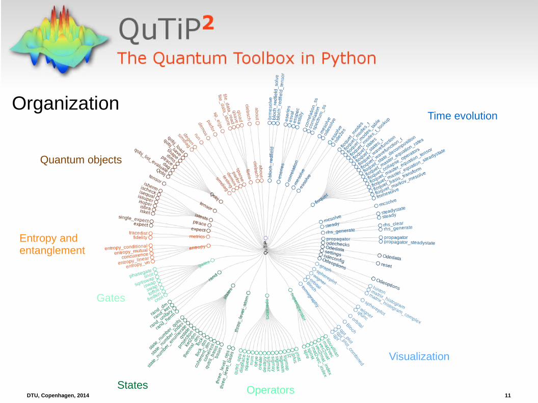
OrganizationTime evolution

Visualization

Gates

OperatorsStates

Quantum objects

Entropy andentanglement


Evolution of quantum systems

Typical simulation work flow:

i. Define parameters that characterize the system

ii. Create Qobj instances for operators and states

iii. Create Hamiltonian, initial state andcollapse operators, if any

iv. Choose a solver and evolve the system

v. Post-process, visualize the data, etc.

Available evolution solvers:

– Unitary evolution: Schrödinger and von Neumann equations

– Lindblad master equations

– Monte-Carlo quantum trajectory method

– Bloch-Redfield master equation

– Floquet-Markov master equation

– Propagators

The main use of QuTiP is quantum evolution. A number of solvers are available.


Lindblad master equation

Equation of motion for the density matrix for a quantum system that interacts with its environment:

How do we solve this equation numerically?

I. Construct the matrix representation of all operatorsII. Evolve the ODEs for the unknown elements in the density matrixIII. For example, calculate expectation values for some selected operators for each


Lindblad master equation

Equation of motion for the density matrix for a quantum system that interacts with its environment:

How do we solve this equation numerically in QuTiP?

from qutip import *

psi0 = ... # initial stateH = ... # system Hamiltonian c_op_list = [...] # collapse operatorse_op_list = [...] # expectation value operators

tlist = linspace(0, 10, 100)result = mesolve(H, psi0, tlist, c_op_list, e_op_list)


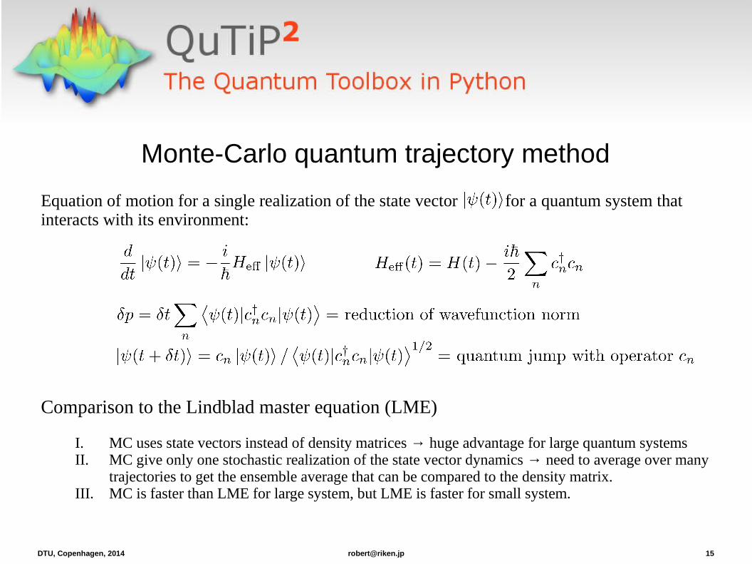
Monte-Carlo quantum trajectory method

Equation of motion for a single realization of the state vector for a quantum system that interacts with its environment:

Comparison to the Lindblad master equation (LME)

I. MC uses state vectors instead of density matrices → huge advantage for large quantum systemsII. MC give only one stochastic realization of the state vector dynamics → need to average over many

trajectories to get the ensemble average that can be compared to the density matrix. III. MC is faster than LME for large system, but LME is faster for small system.


Monte-Carlo quantum trajectory method

Equation of motion for a single realization of the state vector for a quantum system that interacts with its environment:

Comparison to the Lindblad master equation (LME) in QuTiP code:

from qutip import *

psi0 = ... # initial stateH = ... # system Hamiltonian c_list = [...] # collapse operatorse_list = [...] # expectation value operators

tlist = linspace(0, 10, 100)result = mesolve(H, psi0, tlist, c_list, e_list)

from qutip import *

psi0 = ... # initial stateH = ... # system Hamiltonian c_list = [...] # collapse operatorse_list = [...] # expectation value operators

tlist = linspace(0, 10, 100)result = mcsolve(H, psi0, tlist, c_list, e_list, ntraj=500)


Example: Jaynes-Cummings model

Mathematical formulation:

Hamiltonian

Initial state

Time evolution

Expectation values

QuTiP code:from qutip import *N = 10

a = tensor(destroy(N),qeye(2))sz = tensor(qeye(N),sigmaz())s = tensor(qeye(N),destroy(2))wc = wq = 1.0 * 2 * pig = 0.5 * 2 * piH = wc * a.dag() * a - 0.5 * wq * sz + \ 0.5 * g * (a * s.dag() + a.dag() * s)psi0 = tensor(basis(N,1), basis(2,0))tlist = linspace(0, 10, 100)out = mesolve(H, psi0, tlist, [], [a.dag()*a])

from pylab import *plot(tlist, out.expect[0])show()

(a two-level atom in a cavity)

Qobjinstances


Example: time-dependenceMultiple Landau-Zener transitions

from qutip import *

# Parametersepsilon = 0.0delta = 1.0

# Initial state: start in ground statepsi0 = basis(2,0)

# HamiltonianH0 = - delta * sigmaz() - epsilon * sigmax()H1 = - sigmaz()h_t = [H0, [H1, 'A * cos(w*t)']]args = {'A': 10.017, 'w': 0.025*2*pi}

# No dissipationc_ops = []

# Expectation valuese_ops = [sigmax(), sigmay(), sigmaz()]

# Evolve the systemtlist = linspace(0, 160, 500)output = mesolve(h_t, psi0, tlist, c_ops, e_ops, args)

# Process and plot result# ...


Example: open quantum system

from qutip import *

g = 1.0 * 2 * pi # coupling strengthg1 = 0.75 # relaxation rateg2 = 0.25 # dephasing raten_th = 1.5 # environment temperatureT = pi/(4*g)

H = g * (tensor(sigmax(), sigmax()) + tensor(sigmay(), sigmay()))

c_ops = []# qubit 1 collapse operatorssm1 = tensor(sigmam(), qeye(2))sz1 = tensor(sigmaz(), qeye(2))c_ops.append(sqrt(g1 * (1+n_th)) * sm1)c_ops.append(sqrt(g1 * n_th) * sm1.dag())c_ops.append(sqrt(g2) * sz1)# qubit 2 collapse operatorssm2 = tensor(qeye(2), sigmam())sz2 = tensor(qeye(2), sigmaz())c_ops.append(sqrt(g1 * (1+n_th)) * sm2)c_ops.append(sqrt(g1 * n_th) * sm2.dag())c_ops.append(sqrt(g2) * sz2)

U = propagator(H, T, c_ops)

qpt_plot(qpt(U, op_basis), op_labels)

Dissipative two-qubit iSWAP gate

Col

laps

e o p

erat

ors


Visualization● Objectives of visualization in quantum mechanics:

– Visualize the composition of complex quantum states (superpositions and statistical mixtures).

– Distinguish between quantum and classical states. Example: Wigner function.

● In QuTiP:

– Wigner and Q functions, Bloch spheres, process tomography, ...

– most common visualization techniques used in quantum mechanics are implemented


Example notebooks for circuit-QED applications

● IPython notebooks:

– Example notebooks

– Getting started with QuTiP

– Jaynes-Cumming-like models

● Vacuum Rabi oscillations● Single-atom laser● Spectrum of dispersively coupled atom-cavity systems

● Available for download from github:

http://github.com/jrjohansson/qutip-lectures

http://jrjohansson.github.io

http://github.com/jrjohansson/qutip-lectures


Summary● QuTiP: framework for numerical simulations of

quantum systems

– Generic framework for representing quantum states and operators

– Large number of dynamics solvers

● Main strengths:

– Ease of use: complex quantum systems can programmed rapidly and intuitively

– Flexibility: Can be used to solve a wide variety of problems

– Performance: Near C-code performance due to use of Cython for time-critical functions

● Future developments:

– Stochastic master equations?Non-markovian master equations?

More information at: http://www.qutip.org

qutip: quantum toolbox in python - amazon...

Documents