Quenched Invariance Principles

for Random Walks and Elliptic Di↵usions

in Random Media with Boundary

Zhen-Qing Chen⇤, David A. Croydon and Takashi Kumagai†

Dedicated to Professors Martin T. Barlow and Ed Perkins

on the occasion of their 60th birthdays.

January 29, 2014

Abstract

Via a Dirichlet form extension theorem and making full use of two-sided heat kernel estimates,we establish quenched invariance principles for random walks in random environments with aboundary. In particular, we prove that the random walk on a supercritical percolation clusteror amongst random conductances bounded uniformly from below in a half-space, quarter-space,etc., converges when rescaled di↵usively to a reflecting Brownian motion, which has been oneof the important open problems in this area. We establish a similar result for the randomconductance model in a box, which allows us to improve existing asymptotic estimates forthe relevant mixing time. Furthermore, in the uniformly elliptic case, we present quenchedinvariance principles for domains with more general boundaries.

AMS 2000 Mathematics Subject Classification: Primary 60K37, 60F17; Secondary 31C25,35K08, 82C41.

Keywords: quenched invariance principle, Dirichlet form, heat kernel, supercritical percolation,random conductance model

Running title: Quenched invariance principles for random media with a boundary.

1 Introduction

Invariance principles for random walks in d-dimensional reversible random environments date backto the 1980s [27, 40, 42, 43]. The most robust of the early results in this area concerned scalinglimits for the annealed law, that is, the distribution of the random walk averaged over the possiblerealizations of the environment, or possibly established a slightly stronger statement involving some

⇤Research partially supported by NSF Grants NSF Grant DMS-1206276, and NNSFC Grant 11128101.†Research partially supported by the Grant-in-Aid for Scientific Research (B) 22340017 and (A) 25247007.

1

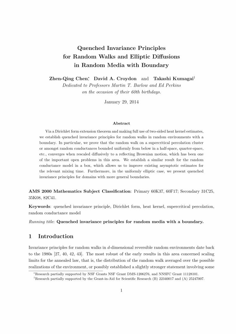
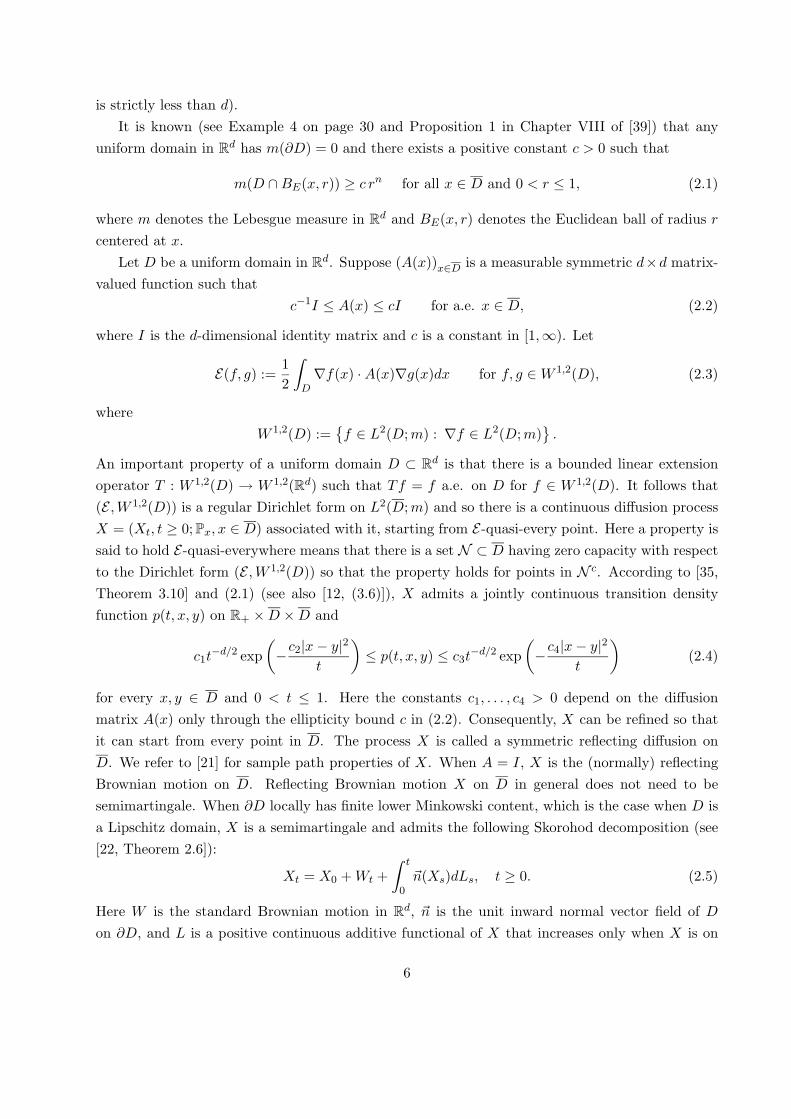
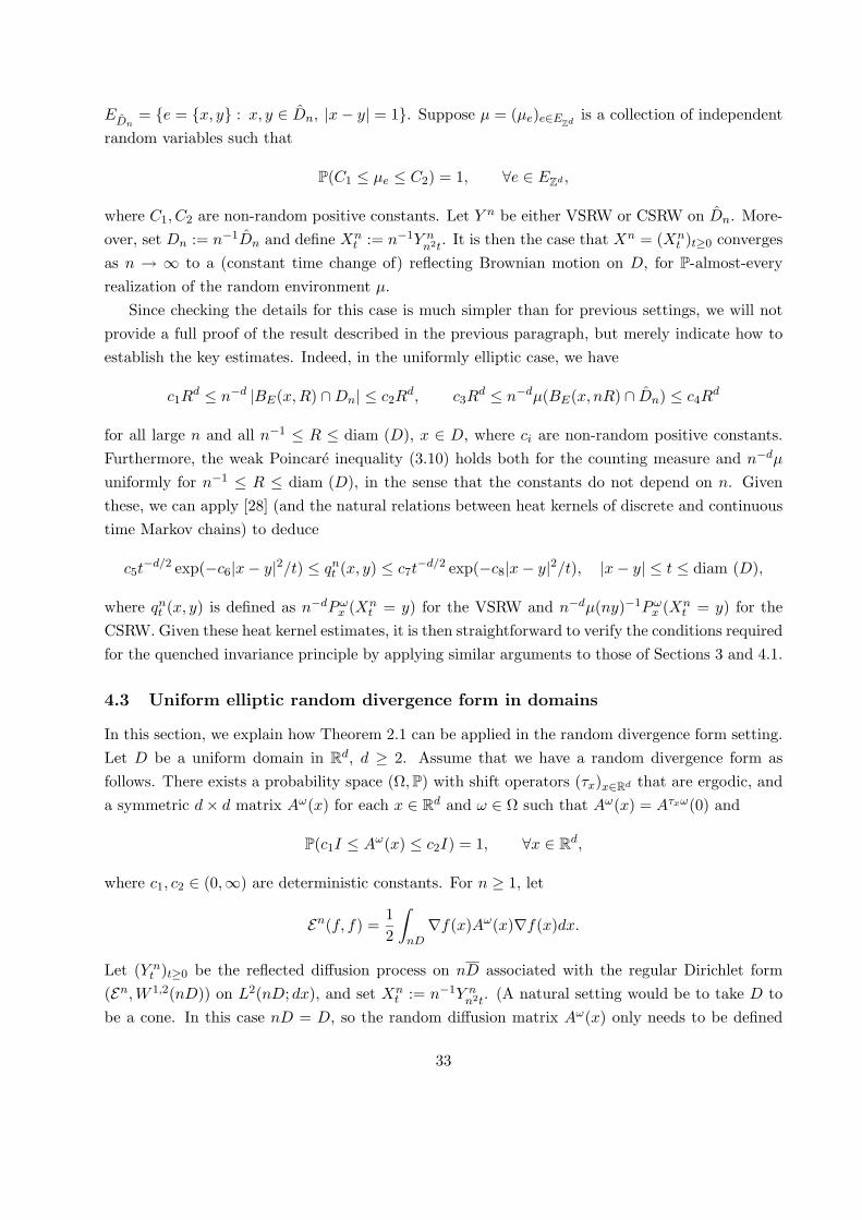
Figure 1: A section of the unique infinite cluster for supercritical percolation on Z2+ with parameter

p = 0.52.

form of convergence in probability. Studying the behavior of the random walks under the quenchedlaw, that is, for a fixed realization of the environment, has proved to be a much more di�culttask, especially when there is some degeneracy in the model. This is because it is often the casethat a typical environment has ‘bad’ regions that need to be controlled. Nevertheless, over the lastdecade significant work has been accomplished in this direction. Indeed, in the important case ofthe random walk on the unique infinite cluster of supercritical (bond) percolation on Zd, buildingon the detailed transition density estimates of [6], a Brownian motion scaling limit has now beenestablished [15, 46, 52]. Additionally, a number of extensions to more general random conductancemodels have also been proved [3, 8, 17, 45].

Whilst the above body of work provides some powerful techniques for overcoming the technicalchallenges involved in proving quenched invariance principles, such as studying ‘the environmentviewed from the particle’ or the ‘harmonic corrector’ for the walk (see [16] for a survey of the recentdevelopments in the area), these are not without their limitations. Most notably, at some point,the arguments applied all depend in a fundamental way on the translation invariance or ergodicityunder random walk transitions of the environment. As a consequence, some natural variationsof the problem are not covered. Consider, for example, supercritical percolation in a half-spaceZ+ ⇥ Zd�1, or possibly an orthant of Zd. Again, there is a unique infinite cluster (Figure 1 showsa simulation of such in the first quadrant of Z2), upon which one can define a random walk. Giventhe invariance principle for percolation on Zd, one would reasonably expect that this process would

2

converge, when rescaled di↵usively, to a Brownian motion reflected at the boundary. After all, as isillustrated in the figure, the ‘holes’ in the percolation cluster that are in contact with the boundaryare only on the same scale as those away from it. However, the presence of a boundary meansthat the translation invariance/ergodicity properties necessary for applying the existing argumentsare lacking. For this reason, it has been one of the important open problems in this area to provethe quenched invariance principle for random walk on a percolation cluster, or amongst randomconductances more generally, in a half-space (see [15, Section B] and [16, Problem 1.9]). Our aimis to provide a new approach for overcoming this issue, and thereby establish invariance principleswithin some general framework that includes examples such as those just described.

The approach of this paper is inspired by that of [19, 20], where the invariance principle forrandom walk on grids inside a given Euclidean domain D is studied. It is shown first in [19] for aclass of bounded domains including Lipschitz domains and then in [20] for any bounded domain D

that the simple random walk converges to the (normally) reflecting Brownian motion on D whenthe mesh size of the grid tends to zero. Heuristically, the normally reflecting Brownian motion isa continuous Markov process on D that behaves like Brownian motion in D and is ‘pushed back’instantaneously along the inward normal direction when it hits the boundary. See Section 2 for aprecise definition and more details. The main idea and approach of [19, 20] is as follows: (i) showthat random walk killed upon hitting the boundary converges weakly to the absorbing Brownianmotion in D, which is trivial; (ii) establish tightness for the law of random walks; (iii) show anysequential limit is a symmetric Markov process and can be identified with reflecting Brownianmotion via a Dirichlet form characterization. In [19, 20], (ii) is achieved by using a forward-backward martingale decomposition of the process and the identification in (iii) is accomplished byusing a result from the boundary theory of Dirichlet form, which says that the reflecting Brownianmotion on D is the maximal Silverstein’s extension of the absorbing Brownian motion in D; see[19, Theorem 1.1] and [23, Theorem 6.6.9].

For quenched invariance principles for random walks in random environments with a boundary,step (i) above can be established by applying a quenched invariance principle for the full-space case.For step (ii), i.e. establishing tightness, the forward-backward martingale decomposition methoddoes not work well with unbounded random conductances. To overcome this di�culty, as well asfor the desire to establish an invariance principle for every starting point, we will make the full useof detailed two-sided heat kernel estimates for random walk on random clusters. In particular, weprovide su�cient conditions for the subsequential convergence that involve the Holder continuityof harmonic functions (see Section 2.2). This continuity property can be verified in examples byusing existing two-sided heat kernel bounds. We remark that the corrector-type methods for full-space models, such as the approach of [15], often require only upper bounds on the heat kernel.Using the Holder regularity, we can further show that any subsequential limit of random walks inrandom environments is a conservative symmetric Hunt process with continuous sample paths. Instep (iii), we can identify the subsequential limit process with the reflecting Brownian motion bya Dirichlet form argument (see Theorem 2.1). In summary, our approach for proving quenched

3

invariance principles for random walks in random environments with a boundary encompasses twonovel aspects: a Dirichlet form extension argument and the full use of detailed heat kernel estimates.

The full generality of the random conductance model to which we are able to apply the aboveargument is presented in Section 3. As an illustrative application of Theorem 2.1, though, we statehere a theorem that verifies the conjecture described above concerning the di↵usive behavior of therandom walk on a supercritical percolation cluster on a half-space, quarter-space, etc. We recallthat the variable speed random walk (VSRW) on a connected (unweighted) graph is the continuoustime Markov process that jumps from a vertex at a rate equal to its degree to a uniformly chosenneighbor (see Section 3 for further details). In this setting, similar results to that stated can beobtained for the so-called constant speed random walk (CSRW), which has mean one exponentialholding times, or the discrete time random walk (see Remark 3.18 below).

Let Z+ := {0, 1, 2, . . . } and R+ := [0,1). Then the following is our main theorem.

Theorem 1.1. Fix d1, d2 2 Z+ such that d1 � 1 and d := d1 +d2 � 2. Let C1 be the unique infinitecluster of a supercritical bond percolation process on Zd1

+ ⇥Zd2, and let Y = (Yt)t�0 be the associatedVSRW. For almost-every realization of C1, it holds that the rescaled process Y n = (Y n

t )t�0, asdefined by

Y nt := n�1Yn2t,

started from Y n0 = xn 2 n�1C1, where xn ! x 2 Rd1

+ ⇥Rd2, converges in distribution to {Xct; t � 0},where c 2 (0,1) is a deterministic constant and {Xt; t � 0} is the (normally) reflecting Brownianmotion on Rd1

+ ⇥ Rd2 started from x.

As an alternative to unbounded domains, one could consider compact limiting sets, replacing Y n

in the previous theorem by the rescaled version of the variable speed random walk on the largestpercolation cluster contained in a box [�n, n]d \ Zd, for example. As presented in Section 4.1,another application of Theorem 2.1 allows an invariance principle to be established in this case aswell, with the limiting process being Brownian motion in the box [�1, 1]d, reflected at the boundary.Consequently, we are able to refine the existing knowledge of the mixing time asymptotics for thesequence of random graphs in question from a tightness result [13] to an almost-sure convergenceone (see Corollary 4.4 below).

Although in the percolation setting we only consider relatively simple domains with ‘flat’ bound-aries, this is mainly for technical reasons so that deriving the percolation estimates in Section 3.1required for our proofs is manageable. Indeed, in the case when we restrict to uniformly ellipticrandom conductances, so that controlling the clusters of extreme conductances is no longer an is-sue, we are able to derive from Theorem 2.1 quenched invariance principles in any uniform domain,the collection of which forms a large class of possibly non-smooth domains that includes (global)Lipschitz domains and the classical van Koch snowflake planar domain as special cases. Theseapplications are discussed in Section 4.2.

Homogenization of reflected SDE/PDE on half-planes and more general domains has beenstudied in various contexts (see, for example, [5, 14, 41, 51, 53]; we refer to [38, 41] and the references

4

therein for the history of homogenization for di↵usions in random environments). In a recent paper[51], Rhodes proves homogenization (as a convergence in product measure in environment andstate space of quenched distribution, which implies an annealed invariance principle) for symmetricreflected di↵usions in upper half spaces. His method is based on the Girsanov formula and a useof subsidiary di↵usions with an invariant probability measure, which is very di↵erent from ours.Although we can also only handle symmetric cases, our methods contribute to this field as well.This is because the analytical part of our results (namely Section 2) holds for the entire class ofuniform domains. Moreover, our results are on the level of quenched invariance principles. Thepresentation of how our techniques can be applied in the uniformly elliptic random divergence formsetting appears in Section 4.3. Note further that in this setting we resolve the open problem on thequenched invariance principle starting from arbitrary starting points posed in [51, pp. 1004–1005].

The remainder of the paper is organized as follows. In Section 2, we introduce an abstractframework for proving invariance principles for reversible Markov processes in a Euclidean domain.This is applied in Section 3 to our main example of a random conductance model in half-spaces,quarter-spaces, etc. The details of the other examples discussed above are presented in Section4. Our results for the random conductance model depend on a number of technical percolationestimates, some of the proofs of which are contained in the appendix that appears at the end ofthis article. The appendix also contains a proof of a generalization of existing quenched invarianceprinciples that allows for arbitrary starting points (previous results have always started the relevantprocesses from the origin, which will not be enough for our purposes).

Finally, in this paper, for a locally compact separable metric space E, we use Cb(E) and C1(E)to denote the space of bounded continuous functions on E and the space of continuous functionson E that vanish at infinity, respectively. The space of continuous functions on E with compactsupport will be denoted by Cc(E). For real numbers a, b, we use a _ b and a ^ b for max{a, b} andmin{a, b}, respectively.

2 Framework

The following definition is taken from Vaisala [55], where various equivalent definitions are dis-cussed. An open connected subset D of Rd is called uniform if there exists a constant C such thatfor every x, y 2 D there is a rectifiable curve � joining x and y in D with length(�) C|x � y|and moreover min {|x� z|, |z � y|} C dist(z, @D) for all points z 2 �. Here dist(z, @D) is theEuclidean distance between the point z and the set @D. Note that a uniform domain with respectto an inner metric is called inner uniform in [35, Definition 3.6].

For example, the classical van Koch snowflake domain in the conformal mapping theory is auniform domain in R2. Every (global) Lipschitz domain is uniform, and every non-tangentiallyaccessible domain defined by Jerison and Kenig in [37] is a uniform domain (see (3.4) of [37]). How-ever, the boundary of a uniform domain can be highly nonrectifiable and, in general, no regularityof its boundary can be inferred (besides the easy fact that the Hausdor↵ dimension of the boundary

5

is strictly less than d).It is known (see Example 4 on page 30 and Proposition 1 in Chapter VIII of [39]) that any

uniform domain in Rd has m(@D) = 0 and there exists a positive constant c > 0 such that

m(D \BE(x, r)) � c rn for all x 2 D and 0 < r 1, (2.1)

where m denotes the Lebesgue measure in Rd and BE(x, r) denotes the Euclidean ball of radius r

centered at x.Let D be a uniform domain in Rd. Suppose (A(x))x2D is a measurable symmetric d⇥d matrix-

valued function such thatc�1I A(x) cI for a.e. x 2 D, (2.2)

where I is the d-dimensional identity matrix and c is a constant in [1,1). Let

E(f, g) :=12

ZDrf(x) ·A(x)rg(x)dx for f, g 2 W 1,2(D), (2.3)

whereW 1,2(D) :=

�f 2 L2(D;m) : rf 2 L2(D;m)

.

An important property of a uniform domain D ⇢ Rd is that there is a bounded linear extensionoperator T : W 1,2(D) ! W 1,2(Rd) such that Tf = f a.e. on D for f 2 W 1,2(D). It follows that(E ,W 1,2(D)) is a regular Dirichlet form on L2(D;m) and so there is a continuous di↵usion processX = (Xt, t � 0; Px, x 2 D) associated with it, starting from E-quasi-every point. Here a property issaid to hold E-quasi-everywhere means that there is a set N ⇢ D having zero capacity with respectto the Dirichlet form (E ,W 1,2(D)) so that the property holds for points in N c. According to [35,Theorem 3.10] and (2.1) (see also [12, (3.6)]), X admits a jointly continuous transition densityfunction p(t, x, y) on R+ ⇥D ⇥D and

c1t�d/2 exp

✓�c2|x� y|2

t

◆ p(t, x, y) c3t

�d/2 exp✓�c4|x� y|2

t

◆(2.4)

for every x, y 2 D and 0 < t 1. Here the constants c1, . . . , c4 > 0 depend on the di↵usionmatrix A(x) only through the ellipticity bound c in (2.2). Consequently, X can be refined so thatit can start from every point in D. The process X is called a symmetric reflecting di↵usion onD. We refer to [21] for sample path properties of X. When A = I, X is the (normally) reflectingBrownian motion on D. Reflecting Brownian motion X on D in general does not need to besemimartingale. When @D locally has finite lower Minkowski content, which is the case when D isa Lipschitz domain, X is a semimartingale and admits the following Skorohod decomposition (see[22, Theorem 2.6]):

Xt = X0 + Wt +Z t

0~n(Xs)dLs, t � 0. (2.5)

Here W is the standard Brownian motion in Rd, ~n is the unit inward normal vector field of D

on @D, and L is a positive continuous additive functional of X that increases only when X is on

6

the boundary, that is, Lt =R t0 1{Xs2@D}dLs for t � 0. Moreover, it is known that the reflecting

Brownian motion spends zero Lebesgue amount of time at the boundary @D. These together with(2.5) justify the heuristic description we gave in the introduction for the reflecting Brownian motionin D.

2.1 Convergence to reflecting di↵usion

In this subsection, D is a uniform domain in Rd and X is a reflecting di↵usion process on D associ-ated with the Dirichlet form (E ,W 1,2(D)) on L2(D;m) given by (2.3). Denote by (XD, PD

x , x 2 D)the subprocess of X killed on exiting D. It is known (see, e.g., [23]) that the Dirichlet form of XD

on L2(D;m) is (E ,W 1,20 (D)), where

W 1,20 (D) :=

�f 2 W 1,2(D) : f = 0 E-quasi-everywhere on @D

.

Suppose that {Dn; n � 1} is a sequence of Borel subsets of D such that each Dn supportsa measure mn that converges vaguely to the Lebesgue measure m on D. The following resultplays a key role in our approach to the quenched invariance principle for random walks in randomenvironments with boundary.

Theorem 2.1. For each n 2 N, let (Xn, Pnx, x 2 Dn) be an mn-symmetric Hunt process on Dn.

Assume that for every subsequence {nj}, there exists a sub-subsequence {nj(k)} and a continu-ous conservative m-symmetric strong Markov process ( eX, ePx, x 2 D) such that the following threeconditions are satisfied:

(i) for every xnj(k)! x with xnj(k)

2 Dnj(k), Pnj(k)

xnj(k)converges weakly in D([0,1), D) to ePx;

(ii) eXD, the subprocess of eX killed upon leaving D, has the same distribution as XD;

(iii) the Dirichlet form (E , F) of eX on L2(D;m) has the properties that

C ⇢ F and E(f, f) C0 E(f, f) for every f 2 C, (2.6)

where C is a core for the Dirichlet form (E ,W 1,2(D)) and C0 2 [1,1) is a constant.

It then holds that for every xn ! x with xn 2 Dn, (Xn, Pnxn

) converges weakly in D([0,1), D) to(X, Px).

Proof. With both eX and X being m-symmetric Hunt processes on D, it su�ces to show thattheir corresponding (quasi-regular) Dirichlet forms on L2(D;m) are the same; that is (eE , eF) =(E ,W 1,2(D)). Condition (iii) immediately implies that W 1,2(D) ⇢ eF and

eE(f, f) C0E(f, f) for every f 2 W 1,2(D).

7

Next, observe that since eX is a di↵usion process admitting no killings, its associated Dirichlet formis strongly local. Thus for every u 2 eF , eE(u, u) = 1

2eµhui(D), where eµhui is the energy measurecorresponding to u. By the proof of [47, Proposition on page 389] ,

eµhui(dx) C0ru(x)A(x)ru(x)dx cC0|ru(x)|2dx on D for every u 2 W 1,2(D).

This in particular implies that

eµhui(@D) = 0 for u 2 W 1,2(D). (2.7)

On the other hand, by the strong local property of eµhui and the fact that eXD has the samedistribution as XD, we have that every bounded function in eF – the collection of which we denoteby eFb – is locally in W 1,2

0 (D) and

1D(x)eµhui(dx) = 1D(x)ru(x)A(x)ru(x)dx for u 2 eFb. (2.8)

This together with (2.7) implies that eE(u, u) = E(u, u) for every bounded u 2 W 1,2(D), and hencefor every u 2 W 1,2(D). Furthermore, (2.8) implies that for u 2 eFb,

RD |ru(x)|2dx < 1 and so

u 2 W 1,2(D). Consequently we have eF ⇢ W 1,2(D) and thus (eE , eF) = (E ,W 1,2(D)).

Remark 2.2. (i) Note that if (Xnt )t�0 is conservative for each n 2 N and {Pnj(k)

xnj(k)} is tight, then

X is conservative.(ii) Theorem 2.1 can be viewed as a variation of [19, Theorem 1.1]. The di↵erence is that in [19,Theorem 1.1], the constant C0 in (2.6) is assumed to be 1 but the limiting process eX only need tobe Markov and does not need to be continuous a priori, while for Theorem 2.1, the condition on theconstant C0 is weaker but we need to assume a priori that the limit process eX is continuous.

2.2 Su�cient condition for subsequential convergence

In this subsection, we give some su�cient conditions for the subsequential convergence of {Xn}; inother words, su�cient conditions for (i) in Theorem 2.1. For simplicity, we assume that 0 2 Dn forall n � 1 throughout this section, though note this restriction can easily be removed.

We start by introducing our first main assumption, which will allow us to check an equi-continuity property for the �-potentials associated with the elements of {Xn} (see Proposition 2.4below). In the statement of the assumption, we suppose that (�n)n�1 is a decreasing sequence in[0, 1] with limn!1 �n = 0 and such that |x� y| � �n for all distinct x, y 2 Dn. (When �n ⌘ 0, thiscondition always holds. However, our assumption will give an additional restriction.) We denoteby ⌧A(Xn) the first exit time of the process Xn from the set A.

Assumption 2.3. There exist c1, c2, c3,�, � 2 (0,1), N0 2 N such that the following hold for alln � N0, x0 2 BE(0, c1n1/2), and �1/2

n r 1.

(i) For all x 2 BE(x0, r/2) \Dn,

Enx

⇥⌧BE(x0,r)\Dn

(Xn)⇤ c2r

�.

8

(ii) If hn is bounded in Dn and harmonic (with respect to Xn) in a ball BE(x0, r), then

|hn(x)� hn(y)| c3

✓|x� y|

r

◆�

khnk1 for x, y 2 BE(x0, r/2) \Dn.

Define for � > 0 the �-potential

U�nf(x) = En

x

Z 1

0e��tf(Xn

t ) dt for x 2 Dn.

Proposition 2.4. Under Assumption 2.3 there exist C = C� 2 (0,1) and �0 2 (0,1) such thatthe following holds for any bounded function f on Dn, for any n � N0 and any x, y 2 Dn such thatx 2 BE(0, c1n1/2) and |x� y| < 1/4:

|U�nf(x)� U�

nf(y)| C|x� y|�0kfk1. (2.9)

In particular, we have

lim�!0

supn�N0

supx,y2Dn\BE(0,c1n1/2):

|x�y|<�

|U�nf(x)� U�

nf(y)| = 0. (2.10)

Proof. The proof is similar to that of [11, Proposition 3.3]. Fix x0 2 BE(0, c1n1/2) \ Dn, let1 � r � �1/2

n , and suppose x, y 2 BE(x0, r/2). Set ⌧nr := ⌧BE(x0,r)\Dn

(Xn). By the strong Markovproperty,

U�nf(x) = En

x

Z ⌧nr

0e��tf(Xn

t ) dt + Enx

h(e��⌧n

r � 1)U�nf(Xn

⌧nr)i

+ Enx

hU�

nf(Xn⌧nr)i

= I1 + I2 + I3,

and similarly when x is replaced by y. We have by Assumption 2.3(i) that

|I1| kfk1Enx⌧n

r c2r�kfk1,

and by noting kU�nfk1 1

�kfk1 that

|I2| �Enx⌧n

r kU�nfk1 c2r

�kfk1.

Similar statements also hold when x is replaced by y. So,���U�nf(x)� U�

nf(y)��� 4c2r

�kfk1 +���En

xU�nf(Xn

⌧nr)� En

yU�nf(Xn

⌧nr)��� . (2.11)

But z ! Enz U�

nf(Xn⌧nr) is bounded in Rd and harmonic in BE(x0, r), so by Assumption 2.3(ii), the

second term in (2.11) is bounded by c3(|x � y|/r)�kU�nfk1. So by kU�

nfk1 1�kfk1 again, we

have ���U�nf(x)� U�

nf(y)��� c

✓r� + ��1

✓|x� y|

r

◆�◆kfk1 for x, y 2 BE(x0, r/2). (2.12)

9

Now, for distinct x, y 2 Dn with x 2 BE(0, c1n1/2) and (�1/2n )2 |x� y| < 1/4 (note that since

|x � y| � �n for distinct x and y, the first inequality always hold), let x0 = x and r = |x � y|1/2.Then �n r < 1/2 and y 2 BE(x0, r/2) (because |x0 � y| = r2 < r/2). Thus we can apply (2.12)to obtain

���U�nf(x)� U�

nf(y)��� c

⇣|x� y|�/2 + ��1|x� y|�/2

⌘kfk1

c(1 + ��1)|x� y|(�^�)/2kfk1.

So (2.9) holds with C = c(1 + ��1) and �0 = (� ^ �)/2. The result at (2.10) is immediate from(2.9).

We note that with an additional mild condition, we can further obtain equi-Holder continuityof the associated semigroup. (The next proposition will only be used in the proof of Theorem 3.13below.) Set BR := BE(0, R) \ Dn for R 2 [2,1). Denote by Xn,BR the subprocess of Xn killedupon exiting BR, and {Pn,BR

t ; t � 0} the transition semigroup of Xn,BR . (When R = 1, we set(Pn

t )t�0 := (Pn,B1t )t�0, i.e. the semigroup of Xn itself.) For p 2 [1,1], we use k · kp,n,R to denote

the Lp-norm with respect to mn on BR.

Proposition 2.5. Let R 2 [2,1] and t > 0. Suppose there exist c1 > 0 and N1 2 N (that maydepend on R and t) such that for every g 2 L1(BR,mn),

kPn,BRt gk1,n,R c1kgk1,n,R, for all n � N1.

Suppose in addition that Assumption 2.3 holds with Xn,BR and BR in place of Xn and Dn, respec-tively. It then holds that there exist constants c 2 (0,1) and N2 � 1 (that also may depend on R

and t) such that ���Pn,BRt f(x)� Pn,BR

t f(y)��� c2|x� y|�0kfk2,n,R,

for every n � N2, f 2 L2(BR;mn), and mn-a.e. x, y 2 BR/2 with |x � y| < 1/4. Here �0 is theconstant of Proposition 2.4.

Proof. We follow [11, Proposition 3.4]. For notational simplicity, we drop the su�ces n � N0 andBR throughout the proof. Using spectral representation theorem for self-adjoint operators, thereexist projection operators Eµ = En,R

µ on the space L2(BR;mn) such that

f =Z 1

0dEµ(f), Ptf =

Z 1

0e�µt dEµ(f), U�f =

Z 1

0

1� + µ

dEµ(f). (2.13)

Defineh =

Z 1

0(� + µ)e�µt dEµ(f).

Since supµ(� + µ)2e�2µt c, we have

khk22 =

Z 1

0(� + µ)2e�2µt dhEµ(f), Eµ(f)i c

Z 1

0dhEµ(f), Eµ(f)i = ckfk2

2,

10

where for f, g 2 L2, hf, gi is the inner product of f and g in L2. Thus h is a well defined functionin L2.

Now, suppose g 2 L1. By the assumption, kPtgk1 ckgk1, from which it follows that kPtgk2 ckgk1. Since supµ(� + µ)e�µt/2 c, using Cauchy-Schwarz we have

hh, gi =Z 1

0(� + µ)e�µt dhEµ(f), gi

✓Z 1

0(� + µ)e�µt dhEµ(f), f)i

◆1/2✓Z 1

0(� + µ)e�µt dhEµ(g), gi

◆1/2

c

✓Z 1

0dhEµ(f), fi

◆1/2✓Z 1

0e�µt/2 dhEµ(g), gi

◆1/2

= ckfk2kPt/2gk2 c0kfk2kgk1.

Taking the supremum over g 2 L1 with L1 norm less than 1, this yields khk1 ckfk2. Finally, by(2.13),

U�h =Z 1

0e�µt dEµ(f) = Ptf, a.e.,

and so the Holder continuity of Ptf follows from Proposition 2.4.)

Let D(R+, D) be the space of right continuous functions on R+ having left limits and takingvalues in D that is equipped with the Skorohod topology. For t � 0, we use Xt to denote thecoordinate projection map on D(R+, D); that is, Xt(!) = !(t) for ! 2 D(R+, D). For subsequentialconvergence to a di↵usion, we need the following.

Assumption 2.6. (i) For any sequence xn ! x with xn 2 Dn, {Pnxn} is tight in D(R+, D).

(ii) For any sequence xn ! x with xn 2 Dn and any " > 0,

lim�!0

lim supn!1

Pnxn

(J(Xn, �) > ") = 0,

where J(X, �) :=R10 e�u

�1 ^ sup�tu |Xt �Xt��|

�du.

We need the following well-known fact (see, for example [7, Lemma 6.4]) in the proof of Propo-sition 2.8. For readers’ convenience, we provide a proof here.

Lemma 2.7. Let K be a compact subset of Rd. Suppose f and fk, k 2 N, are functions on K suchthat limk!1 fk(yk) = f(y) whenever yk 2 K converges to y. Then f is continuous on K and fk

converges to f uniformly on K.

Proof. We first show that f is continuous on K. Fix x0 2 K. Let xk be any sequence in K thatconverges to it. Since limi!1 fi(x) = f(x) for every x 2 K, there is a sequence nk 2 N thatincreases to infinity so that |fnk(xk)�f(xk)| 2�k for every k � 1. Since limk!1 fnk(xk) = f(x0),it follows that limk!1 |f(x0)� f(xk)| = 0. This shows that f is continuous at x0 and hence on K.

11

We next show that fk converges uniformly to f on K. Suppose not. Then there is " > 0 so thatfor every k � 1, there are nk � k and xnk 2 K so that |fnk(xnk)�f(xnk)| > ". Since K is compact,by selecting a subsequence if necessary, we may assume without loss of generality that xnk ! x0 2K. As limk!1 fnk(xnk) = f(x0) by the assumption, we have lim infk!1 |f(x0)�f(xnk)| � ". Thiscontradicts to the fact that f is continuous on K.

Now, applying the argument in [7, Section 6], we can prove that any subsequential limit ofthe laws of Xn under Pn

xnis the law of a symmetric di↵usion. For this, we need to introduce a

projection map from D to Dn. For each n � 1, let �n : D ! Dn be a map that projects eachx 2 D to some �n(x) 2 Dn that minimizes |x � y| over y 2 Dn (if there is more than one suchpoint that does this, we choose and fix one). If needed, we extend a function f defined on Dn tobe a function on D by setting f(x) = f(�n(x)). Note that each Dn supports the measure mn thatconverges vaguely to m. This implies that for each x 2 D and r > 0, there is an N � 1 so that�n(x) 2 BE(x, r) for every n � N . From this, one concludes that

�n(xn) ! x0 for every sequence xn 2 D that converges to x0. (2.14)

Proposition 2.8. Suppose that Assumptions 2.3 and 2.6 hold and that {Xn, Pnx, x 2 Dn} is

conservative for su�ciently large n. For every subsequence {nj}, there exists a sub-subsequence{nj(k)} and a continuous conservative m-symmetric Hunt process ( eX, ePx, x 2 D) such that forevery xnj(k)

! x, Pnj(k)xnj(k) converges weakly in D([0,1), D) to ePx.

Proof. For notational simplicity, let us relabel the subsequence as {n}. We first claim that thereexists a (sub-)subsequence {nj} such that U�

njf converges uniformly on compact sets for each � > 0

and f 2 Cb(D). Indeed, let {�i} be a dense subset of (0,1) and {fk} a sequence of functions inCb(D) such that kfkk1 1 and whose linear span is dense in (Cb(D), k · k1). For fixed m and i,by Proposition 2.4 and the Ascoli-Arzela theorem, there is a subsequence of U�i

n fk that convergesuniformly on compact sets. By a diagonal selection procedure, we can choose a subsequence {nj}such that U�i

njfk converges uniformly on compact sets for every m and i to a Holder continuous

function which we denote as U�ifk. Noting that

U�n � U�

n = (� � �)U�nU�

n , kU�nk1!1 1

�, kU�

n � U�n k1!1 � � �

��, (2.15)

a careful limiting argument shows that U�nj

f converges uniformly on compact sets, say to U�f , forany � > 0 and any continuous function f , and (2.15) holds as well for {U�}. By the equi-continuityof U�

njf , we also have U�

njf(xnj ) ! U�f(x) for each xnj 2 Dnj that converges to x 2 D.

We next claim that Pnjxnj

converges weakly, say to ePx. Indeed, by Assumption 2.6(i), {Pnjxnj

} istight, so it su�ces to show that any two limit points agree. Let P0 and P00 be any two limit points.Then, one sees that

E0Z 1

0e��sf(Xs)ds

�= U�f(x) = E00

Z 1

0e��sf(Xs)ds

�,

12

for any f 2 Cb(D). So, by the uniqueness of the Laplace transform,

E0[f(Xs)] = E00[f(Xs)]

for almost all s � 0 and hence for every s � 0 since s ! Xs is right continuous. So the one-dimensional distributions of Xt under P0 and P00 are the same. Set Psf(x) := E0f(Xs). We haveP

njs f(xnj ) ! Psf(x) for every sequence xnj 2 Dnj that converges to x. Recall the restriction

map �n introduced proceeding the statement of this theorem. It follows from (2.14) that Pnjs (f �

�nj )(ynj ) ! Psf(y) for every sequence ynj 2 D that converges to y. Thus by Lemma 2.7, Pnjs (f �

�nj ) converges to Psf uniformly on compact subsets of D and Psf 2 Cb(D) for every f 2 Cc(D).For f, g 2 Cc(D) and 0 s < t, by the Markov property of X under Pnj

xnj,

Enjxnj

[g(Xs)f(Xt)] = Enjxnj

⇥((Pn

t�sf)g)(Xs)⇤

= Enjxnj

[((Pt�sf)g)(Xs)] + Enjxnj

⇥((Pn

t�sf � Pt�sf)g)(Xs)⇤.

The first term of the right-hand side converges to E0[((Pt�sf)g)(Xs)] by the above proof, whilethe second term goes to 0 since P

njt�sf ! Pt�sf uniformly on compact sets. Repeating this, we

conclude that for every k � 1 and every 0 < s1 < s2 < · · · < sk and fj 2 Cc(D),

E024 kY

j=1

fj(Xsj )

35 = E00

24 kY

j=1

fj(Xsj )

35 = Ps1 (f1Ps2�s1(f2Ps3�s2(f3 . . . ))) (x). (2.16)

This proves that the finite dimensional distributions of X under P0 and P00 are the same. Conse-quently, P0 = P00, which we now denote as ePx. Moreover, (2.16) shows that (X, ePx, x 2 D) is aMarkov process with transition semigroup {Pt, t � 0}.

Next we show that {ePx : x 2 D} is a strong Markov process. Note that X is conservative withePx(X0 = x) = 1, and under Assumption 2.6(ii), Xt is continuous a.s. under ePx. We also havePtf 2 Cb(D) for f 2 Cc(D). It is easy to deduce from these properties and (2.16) that for everyf 2 Cc(D) and every stopping time T ,

Ex [f(XT+t)|FT+] = Ptf(XT ), x 2 D.

See the proof of Theorem 2.3.1 on p.56 of [24]. From it, one gets the strong Markov property of X

by a standard measure-theoretic argument (see p.57 of [24]). Since X is continuous and has infinitelifetime, this in fact shows that X is a continuous conservative Hunt process.

Finally, for f, g 2 Cc(D), by the convergence of semigroups and vague convergence of measures,it holds that, for every t > 0,

ZDn

(Pnjt f)(x)g(x)mnj (dx) !

ZD

(Ptf)(x)g(x)m(dx).

Since Xnj is mn-symmetric, this readily yields the desired m-symmetry of X.

13

Remark 2.9. Note that we did not use any special properties of the Euclidean metric in this section,so that all the arguments in this section can be extended to a metric measure space without anychanges.

By Theorem 2.1, Remark 2.2 (i) and Proposition 2.8, we see that in order to prove (Xn, Pnxn

)converges weakly to (X, Px) in D([0,1), D) as n ! 1, it su�ces to verify condition (ii), (iii) inTheorem 2.1, vague convergence of the measure mn to m on D, Assumptions 2.3 and 2.6, and theconservativeness of (Xn, Pn

xn) for each n 2 N.

3 Random conductance model in unbounded domains

In this section we will obtain, as a first application of our theorem, a quenched invariance prin-ciple for random walk amongst random conductances on half-spaces, quarter-spaces, etc. Theassumptions we make on the random conductances include the supercritical percolation model,and random conductances bounded uniformly from below and with finite first moments. For themain conclusion, see Theorem 3.17.

Fix d1, d2 2 Z+ such that d1 � 1 and d := d1 + d2 � 2. Define a graph (L, EL) by settingL := Zd1

+ ⇥ Zd2 and EL := {e = {x, y} : x, y 2 L, |x� y| = 1}. Given O ✓ EL, let C1(L,O) be theinfinite connected cluster of (L,O), provided it exists and is unique (otherwise set C1(L,O) := ;).

Let µ = (µe)e2EL be a collection of independent and identically distributed random variableson [0,1), defined on a probability space (⌦, P) such that

p1 := P (µe > 0) > pbondc (Zd), (3.1)

where pbondc (Zd) 2 (0, 1) is the critical probability for bond percolation on Zd. We assume that

there is c > 0 so thatP (µe 2 (0, c)) = 0, (3.2)

andE (µe) < 1. (3.3)

This framework includes the special cases of supercritical percolation (where P (µe = 1) = p1 =1� P (µe = 0)) and the random conductance model with conductances bounded from below (thatis, P (c µe < 1) = 1 for some c > 0) and having finite first moments. For each x 2 L, setµx =

Py⇠x µxy. Set

O1 := {e 2 EL : µe > 0} , C1 := C1(L,O1).

Note that for the random conductance model bounded from below, C1 = L.For each realization of C1, there is a continuous time Markov chain Y = (Yt)t�0 on C1 with

transition probabilities P (x, y) = µxy/µx, and the holding time at each x 2 C1 being the exponentialdistribution with mean µ�1

x . Such a Markov chain is sometimes called a variable speed random

14

walk (VSRW). The corresponding Dirichlet form is (E , L2(C1; ⌫)), where ⌫ is the counting measureon C1 and

E(f, g) =12

Xx,y2C1, x⇠y

(f(x)� f(y))(g(x)� g(y))µxy for f, g 2 L2(C1; ⌫).

The corresponding discrete Laplace operator is LV f(x) =P

y(f(y)� f(x))µxy. For each f, g thathave finite support, we have

E(f, g) = �Xx2C1

(LV f)(x)g(x).

We will establish a quenched invariance principle for Y in Section 3.3, but we first need to derivesome preliminary estimates regarding the geometry of C1 and the heat kernel associated with Y .

3.1 Percolation estimates

In this section, we derive a number of useful properties of the underlying percolation cluster C1.Most importantly, we introduce the concept of ‘good’ and ‘very good’ balls for the model andprovide estimates for the probability of such occurring, see Definition 3.4 and Proposition 3.5below.

Since a variety of percolation models will appear in the course of this paper, let us now makeexplicit that the critical probability for bond/site percolation on an infinite connected graph con-taining the vertex 0 is

pc := inf {p 2 [0, 1] : Pp (0 is in an infinite connected cluster of open bonds/sites) > 0} ,

where Pp is the law of parameter p bond/site percolation on the graph in question. Note inparticular that the critical probability for bond percolation on L is identical to pbond

c (Zd), see [32,Theorem 7.2] (which is the bond percolation version of a result originally proved as [33, TheoremA]). Recall

O1 := {e 2 EL : µe > 0} , C1 := C1(L,O1).

That C1 is non-empty almost-surely is guaranteed by [10, Corollary to Theorem 1.1] (this coversd � 3, and, as is commented there, the case d = 2 can be tackled using techniques from [36]).

Now, suppose that µ is actually a restriction of independent and identically distributed (underP) random variables (µe)e2EZd , where EZd are the usual nearest-neighbor edges for the integerlattice Zd, and define

O1 := {e 2 EZd : µe > 0} , C1 := C1(Zd, O1).

For su�ciently large K so that

q = q(K) := P(0 < µe < K�1) + P(µe > K) < p1 � pbondc (Zd),

15

and writing OI := {e 2 EZd : µe 2 I} for I ✓ [0,1), we let

OR := O(0,K�1)[(K,1),

OS :=n

e 2 O1 : e \ e0 6= ; for some e0 2 OR

o,

O2 := O1\OS .

We will also define O2 := O2 \ EL, and set C2 := C1(L,O2) – the next lemma will guarantee thatthis set is non-empty almost-surely.

To represent the set of ‘holes’, let H := C1\C2. Moreover, for x 2 C1, let H(x) be the connectedcomponent of C1\C2 containing x. The following lemma provides control on the size of thesecomponents. Since its proof is a somewhat technical adaptation to our setting of that used toestablish [3, Lemma 2.3], which dealt with the whole Zd model, we defer this to the appendix.Note, though, that in the percolation case (i.e. when µe are Bernoulli random variables) or theuniformly elliptic random conductor case, the proof of the result is immediate; indeed, for largeenough K, we have that O2 = O1, and so H = ;.

Lemma 3.1. For su�ciently large K, the following holds.(i) All the connected components of H are finite. Furthermore, there exist constants c1, c2 suchthat: for each x 2 L,

P (x 2 C1 and diam(H(x)) � n) c1e�c2n,

where diam denotes the diameter with respect to the `1 metric on Zd.(ii) There exists a constant ↵ such that, P-a.s., for large enough n, the volume of any hole inter-secting the box [�n, n]d \ L is bounded above by (log n)↵.

In what follows, we will need to make comparisons between two graph metrics on (C1,O1), andthe Euclidean metric. The first of these, d1, will simply be defined to be the shortest path metricon (C1,O1), considered as an unweighted graph. To define the second metric, d1, we follow [8] bydefining edge weights

t(e) := CA ^ µ�1/2e ,

where CA < 1 is a deterministic constant, and then letting d1 be the shortest path metric on(C1,O1), considered as a weighted graph (in [8], the analogous metric was denoted d). We notethat the latter metric on C1 satisfies

�C�2

A _ µ{y,z}� ��d1(x, y)� d1(x, z)

��2 1,

for any x, y, z 2 C1 with {y, z} 2 O1. Observe that, since the weights t(e) are bounded above by CA,we immediately have that d1 is bounded above by CAd1, Hence the following lemma establishes bothd1 and d1 are comparable to the Euclidean one. An easy consequence of this is the comparabilityof balls in the di↵erent metrics, see Lemma 3.3. The proofs of both these results are deferred tothe appendix.

16

Lemma 3.2. There exist constants c1, c2, c3 such that: for R � 1,

supx,y2L:|x�y|R

P (x, y 2 C1 and d1(x, y) � c1R) c2e�c3R, (3.4)

and also, for every x, y 2 L,

P�x, y 2 C1 and d1(x, y) c�1

1 |x� y|� c2e

�c3|x�y|. (3.5)

Lemma 3.3. There exist constants c1, c2, c3, c4 such that: for every x 2 L, R � 1,

P�{x 2 C1} \

�C1 \BE(x, c1R) ✓ B1(x,R) ✓ B1(x,CAR) ✓ BE(x, c2R)

c� c3e�c4R,

where B1(x, R) is a ball in the metric space (C1, d1), B1(x,R) is a ball in (C1, d1), and BE(x, R) isa Euclidean ball.

We continue by adapting a definition for ‘good’ and ‘very good’ balls from [3]. In preparationfor this, we define µ0

e := 1{e2O1}, set µ0x :=

Py2L µ0

{x,y} for x 2 L, and then extend µ0 to a measureon L. Moreover, we set � := 1� 2(1 + d)�1.

Definition 3.4. (i) Let CV , CP , CW , CR, CD be fixed strictly positive constants. We say the pair(x,R) 2 C1 ⇥ R+ is good if:

B1(x,C�1A r) ✓ B1(x, r) ✓ B1(x,CDr), 8r � R, (3.6)

|y � z| � C�1R R, 8y 2 B1(x,R/2), z 2 B1(x, 8R/9)c, (3.7)

CV Rd µ0(B1(x,R)), (3.8)

diam(H(y)) R�, 8y 2 BE(x,R) \ C1, (3.9)

and the weak Poincare inequalityX

y2B1(x,R)

�f(y)� fB1(x,R)

�2µ0

y CP R2X

y,z2B1(x,CW R):{y,z}2O1

|f(y)� f(z)|2 (3.10)

holds for every f : B1(x, CW R) ! R. (Here fB1(x,R) is the value which minimizes the left-handside of (3.10)).(ii) We say a pair (x, R) 2 C1⇥R+ is very good if: there exists N = N(x,R) such that (y, r) is goodwhenever y 2 B1(x, R) and N r R. We can always assume that N � 2. Moreover, if N M ,we will say that (x, R) is M -very good.(iii) Let ↵ 2 (0, 1]. For x 2 C1, we define R(↵)

x to be the smallest integer M such that (x, R) isR↵-very good for all R � M . We set R(↵)

x = 0 if x 62 C1.

The following proposition, which is an adaptation of [3, Proposition 2.8], provides bounds forthe probabilities of these events and for the distribution of R(↵)

x .

17

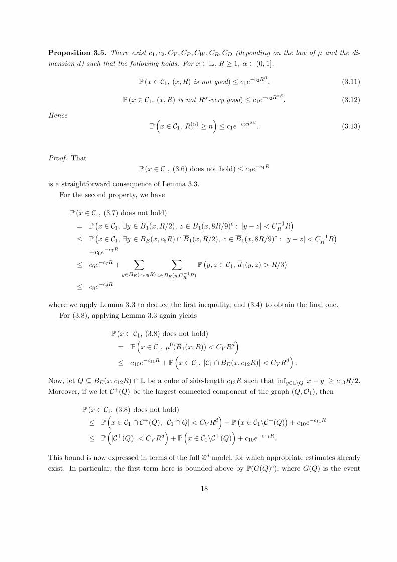
Proposition 3.5. There exist c1, c2, CV , CP , CW , CR, CD (depending on the law of µ and the di-mension d) such that the following holds. For x 2 L, R � 1, ↵ 2 (0, 1],

P (x 2 C1, (x,R) is not good) c1e�c2R�

, (3.11)

P (x 2 C1, (x,R) is not R↵-very good) c1e�c2R↵�

. (3.12)

HenceP⇣x 2 C1, R(↵)

x � n⌘ c1e

�c2n↵�. (3.13)

Proof. ThatP (x 2 C1, (3.6) does not hold) c3e

�c4R

is a straightforward consequence of Lemma 3.3.For the second property, we have

P (x 2 C1, (3.7) does not hold)

= P�x 2 C1, 9y 2 B1(x,R/2), z 2 B1(x, 8R/9)c : |y � z| < C�1

R R�

P�x 2 C1, 9y 2 BE(x, c5R) \B1(x,R/2), z 2 B1(x, 8R/9)c : |y � z| < C�1

R R�

+c6e�c7R

c6e�c7R +

Xy2BE(x,c5R)

Xz2BE(y,C�1

R R)

P�y, z 2 C1, d1(y, z) > R/3

�

c8e�c9R

where we apply Lemma 3.3 to deduce the first inequality, and (3.4) to obtain the final one.For (3.8), applying Lemma 3.3 again yields

P (x 2 C1, (3.8) does not hold)

= P⇣x 2 C1, µ0(B1(x,R)) < CV Rd

⌘

c10e�c11R + P

⇣x 2 C1, |C1 \BE(x, c12R)| < CV Rd

⌘.

Now, let Q ✓ BE(x, c12R) \ L be a cube of side-length c13R such that infy2L\Q |x � y| � c13R/2.Moreover, if we let C+(Q) be the largest connected component of the graph (Q,O1), then

P (x 2 C1, (3.8) does not hold)

P⇣x 2 C1 \ C+(Q), |C1 \Q| < CV Rd

⌘+ P

�x 2 C1\C+(Q)

�+ c10e

�c11R

P⇣|C+(Q)| < CV Rd

⌘+ P

⇣x 2 C1\C+(Q)

⌘+ c10e

�c11R.

This bound is now expressed in terms of the full Zd model, for which appropriate estimates alreadyexist. In particular, the first term here is bounded above by P(G(Q)c), where G(Q) is the event

18

that |C+(Q)| � 12P(0 2 C1)|Q| (recall that C1 := C1(Zd, O1)). Consequently, by simply translating

the relevant part of [3, Lemma 2.6] to our setting (taking K = 1), we obtain that it is boundedabove by c13e�c14R� . That the second term is bounded above by c15e�c16R can be established byapplying [6, Lemma 2.8].

To check the fourth property, we simply note

P (x 2 C1, (3.9) does not hold) X

y2BE(x,R)\LP⇣y 2 C1, diam(H(y)) > R�

⌘,

which may be bounded above by c17e�c18R� by applying Lemma 3.1.Finally, for the Poincare inequality, we will apply [6, Proposition 2.12]. In particular, this

result yields that if Q is a cube of side-length 2R contained in L, C+(Q) is the largest connectedcomponent of the graph (Q,O1), and H(Q) is the event that

mina

Xy2C+(Q)

(f(y)� a)2 µ0y CR2

Xy,z2C+(Q):{y,z}2O1

|f(y)� f(z)|2

for every f : C+(Q) ! R, then P(H(Q)c) c19e�c20R� . Furthermore, it is clear that if H(Q) holdsand also B1(x, R) ✓ C+(Q) ✓ B1(x, c21R), then (3.10) holds. This means that

P (x 2 C1, (3.10) does not hold)

c22e�c23R�

+ P�{x 2 C1} \

�B1(x,R) ✓ C+(Q) ✓ B1(x, c21R)

c�,

where Q is chosen such that BE(x,R)\L ✓ Q. Noting as above that P(x 2 C1\C+(Q)) c24e�c25R,at the expense of adjusting constants, we may replace {x 2 C1} by {x 2 C1 \ C+(Q)} in the abovebound. On the event {x 2 C1 \ C+(Q)} \ {B1(x,R) ✓ C+(Q)}c, it is elementary to check thatB1(x,R) 6✓ BE(x,R), which is impossible. Since C+(Q) ✓ BE(x, 2R), we have thus shown that

P (x 2 C1, (3.10) does not hold)

c26e�c27R�

+ P ({x 2 C1} \ {BE(x, 2R) ✓ B1(x, cR)}c) .

By applying Lemma 3.3 once again, this expression is bounded above by c28e�c29R� , and so we havecompleted the proof of (3.11).

Given (3.11), a simple union bound subsequently yields (3.12), and the inequality at (3.13) is astraightforward consequence of this.

Remark 3.6. It only requires a simple argument to check that if (x,R) is good and y 2 C1 satisfiesd1(x, y) � CDR, then

C�1D d1(x, y) d1(x, y) CAd1(x, y)

(cf. [8, Lemma 2.10(a)]).

Finally, we state a bound that allows us to compare ⌫ with ⌫, which is the measure definedsimilarly from the whole Zd model, i.e. uniform measure on C1. Its proof can be found in theappendix.

19

Lemma 3.7. There exists a constant c such that if Q ✓ L is a cube of side length n, then

P⇣⌫(Q)� ⌫(Q) � nd�1(log n)d+1

⌘ cn�2.

3.2 Heat kernel estimates

Let Dn = n�1C1, D = Rd1+ ⇥Rd2 (recall R+ := [0,1)). Let Y be the VSRW on C1, and for a given

realization of C1 = C1(!), ! 2 ⌦, write P!x for the law of Y started from x 2 C1. Moreover, define

Z to be the trace of Y on C2, that is, the time change of Y by the inverse of At =R t0 1(Ys2C2)ds.

Specifically, writing at = inf{s : As > t} for the right-continuous inverse of A, we set

Zt = Yat , t � 0.

Note that unlike Y , the process Z may perform long jumps by jumping over the holes of C2. Ifx 2 C2(!) then we have Z0 = Y0 = x, P!

x -a.s., but otherwise Z0 = Ya0 .Given the percolation estimates of Section 3.1, we can follow [3, Section 4] to establish the

following theorems, which correspond to Proposition 4.7(c) and Theorem 4.11 in [3]. We remarkthat the second of the two results will be used in this paper only for the proof of Theorem 3.12.Since it is the case that, given Proposition 3.5, the proofs are a simple modification of those in [3],we omit them. For the statement of the first result, we set

(R, t) =

8<:

e�R2/t if t > e�1R,

e�R log(R/t) if t < e�1R.

Proposition 3.8. Write ⌧ZA = inf{t : Zt 62 A}, ⌧Y

A = inf{t : Yt 62 A}. There exist constants�, ci 2 (0,1) and random variables (Rx, x 2 L) with

P(Rx � n, x 2 C1) c1e�c2n�

, (3.14)

such that the following holds: for x 2 C1, t > 0 and R � Rx,

P!x (⌧Z

BE(x,R) < t) c3 (c4R, t),

P!x (⌧Y

BE(x,R) < t) c3 (c4R, t).

Theorem 3.9. There exist: constants �, ci 2 (0,1); a set ⌦1 ⇢ ⌦ with P(⌦1) = 1; and randomvariables (Sx, x 2 L) satisfying Sx(!) < 1 for each ! 2 ⌦1 and x 2 C2(!), and

P(Sx � n, x 2 C2) c1e�c2n�

;

20

such that the following statements hold.(a) For x, y 2 C2(!) the transition density of Z, as defined by setting qZ

t (x, y) := P!x (Zt = y),

satisfies

qZt (x, y) c3t

�d/2 exp(�c4|x� y|2/t), t � |x� y| _ Sx,

qZt (x, y) � c5t

�d/2 exp(�c6|x� y|2/t), t � |x� y|3/2 _ Sx.

(b) Further, if x 2 C2(!), t � Sx and B = B2(x, 2p

t) then

qZ,Bt (x, y) � c7t

�d/2 for y 2 B2(x,p

t),

where B2(x,R) is a ball in the (unweighted) graph (C2,O2), and qZ,B is the transition of Z killedon exiting B, i.e. qZ,B

t (x, y) := P!x (Zt = y, ⌧Z

B > t).

Applying Proposition 3.8, we can establish the following, which corresponds to [3, Proposition5.13 (b)]. To state the result, we introduce the rescaled process Y n = (Y n

t )t�0 by setting

Y nt := n�1Yn2t.

Proposition 3.10 (Tightness). Let K,T, r > 0. For P-a.e. !, the following is true: if xn 2Dn, n � 1, x 2 BE(0,K) are such that xn ! x, then

limR!1

lim supn!1

P!nxn

supsT

|Y ns | > R

!= 0, (3.15)

lim�!0

lim supn!1

P!nxn

sup

|s1�s2|�,siT|Y n

s2� Y n

s1| > r

!= 0. (3.16)

In particular, for P-a.e. !, if xn 2 Dn, n � 1, x 2 D are such that xn ! x, under P!nxn

, the familyof processes (Y n

t )t�0, n 2 N is tight in D([0,1), D).

Proof. Since the statement is slightly di↵erent from [3, Proposition 5.13], we sketch the proof. Notethat since xn ! x 2 BE(0,K), then by setting M = K + 1 we have that nxn 2 BE(0, nM) for alln suitably large. Let nR > supn Rnxn . Then, by Proposition 3.8,

P!nxn

supsT

|Y ns | > R

!= P!

nxn

⇣⌧YBE(0,nR) < n2T

⌘ c1 (c2nR, n2T ).

Considering separately the cases 1/n < T/R and 1/n � T/R, we deduce that

P!nxn

supsT

|Y ns | > R

! c3e

�c4R2/T _ e�R.

Since lim supn Rnxn/n lim supn supx2BE(0,Mn) Rx/n < 1, P-a.s., due to the Borel-Cantelli argu-ment using (3.14), we obtain (3.15).

21

We next prove (3.16). Write

p(x, T, �, r) = P!x

sup

|s1�s2|�,siT|Ys2 � Ys1 | > r

!,

so that

P!nxn

sup

|s1�s2|�,siT|Y n

s2� Y n

s1| > r

!= p(nxn, n2T, n2�, nr).

Arguing similarly to the proof of [3, Proposition 5.13], we have

p(nxn, n2T, n2�, 2nr) c exp(�cnT 1/2) + c(T/�) exp(�cr2/�),

providedT 1/2 � n�1R2/3

x , � > n�1r, r � n�1 maxy2BE(nxn,n3/2T 3/4)

Ry. (3.17)

Note that BE(nxn, n3/2T 3/4) ⇢ BE(0, nM + n3/2T 3/4) for large n. If T, r and � are fixed, due tothe Borel-Cantelli argument using (3.14), each of conditions in (3.17) holds when n is large enough.So, for P-a.e. !,

lim supn!1

p(nxn, n2T, n2�, 2nr) c(T/�) exp(�cr2/�),

and (3.16) follows.Using (3.15) and (3.16), we have tightness for {P!

nxn} by [31, Corollary 3.7.4].

We can further establish the following theorems, which correspond to [17, Lemma 5.6, Propo-sition 6.1] and [3, Theorem 7.3]. We denote by (qY

t (x, y))x,y2C1,t>0 the heat kernel associated withY , i.e. for x, y 2 C1, t > 0,

qYt (x, y) := P!

x (Yt = y).

(We recall that the invariant measure of Y is the uniform measure ⌫ on C1).

Proposition 3.11. There exist c1, c2, c3, � 2 (0,1) (non-random) and random variables (Rx, x 2L) with

P(Rx � n, x 2 C1) exp(�c1n�), (3.18)

such that if x, y 2 C1, then

qYt (x, y) c2t

�d/2 for t � (c3 _ 2d1(x, y) _Rx)1/4.

Proof. Note that the corresponding result for Z-process is given in [3, Corollary 4.3]. We need toobtain similar result for Y -process. First, note that because we have Proposition 3.5, the proof of[3, Proposition 4.1 and Corollary 4.3] (with " = 1/4 for simplicity) goes through once (4.7) in [3]is verified. To check [3, (4.7)], we use [8, Theorem 2.3], which can be proved almost identicallyin our case. Note that in [8, Theorem 2.3], the metric d is used, but thanks to Remark 3.6, wecan obtain the same estimates using the metric d1. Finally, using Cauchy-Schwarz, we obtain thedesired inequality.

22

For G ⇢ C1, we define @out(G) to be the exterior boundary of G in the graph (C1,O1), i.e. thosevertices of C1\G that are connected to G by an edge in O1, and set cl(G) = G [ @out(G). We saythat a function h is Y –harmonic in A ⇢ C1 if h is defined on cl(A) and LV h(x) = 0 for x 2 A.

Theorem 3.12 (Elliptic Harnack inequality). There exist random variables (R0x, x 2 L) with

P(x 2 C1, R0x � n) ce�c0n�

,

and a constant CE such that if x0 2 C1, R � R0x0

and h : cl(B1(x0, R)) ! R+ is Y –harmonic onB1 = B1(x0, R), then writing B0

1 = B1(x0, R/2),

supB0

1

h CE infB0

1

h.

Proof. Given Lemma 3.1, the proof is almost identical to that of [3, Theorem 7.3].

3.3 Quenched invariance principle

To prove a quenched invariance principle for Y (see Theorem 3.17 below), we will check the con-ditions of Theorem 2.1 one by one. We choose �n = c2

⇤/n, where c⇤ is a constant that will bechosen later. First, since Xn is a continuous time Markov chain with holding time at x being anexponential random variable of mean µ�1

x , it is conservative. Condition (ii) in Theorem 2.1 is aconsequence of the quenched invariance principle for the whole space (cf. [3]) and the fact thatC1 ✓ C1, which is a consequence of the uniqueness of the infinite percolation clusters in the twosettings. Since in the original papers quenched invariance principles are uniformly stated in termsof the random walk started from the origin, whereas we require such to hold from an arbitrarystarting point, we state the following generalization of existing results. We will suppose that P!

y

refers to the quenched law of the VSRW Y on C1 started from y 2 C1, and Y n refers to the rescaledprocess defined by setting Y n

t := n�1Yn2t. The proof of the result can be found in the appendix.

Theorem 3.13. There exists a deterministic constant c 2 (0,1) such that, for P-a.e !, the laws ofthe processes Y n under P!

nxn, where nxn 2 C1 and xn ! x, converge weakly to the laws of (Bct)t�0,

where (Bt)t�0 is standard Brownian motion on Rd started from x.

Concerning Assumption 2.3(i), we will prove the following: there exist c⇤, c1 2 (0,1) (non-random) and N0(!) such that for all n � N0(!), x0, x 2 BE(0, n1/2) \Dn and c⇤/n1/2 r0 1,

E!x

�⌧BE(x0,r0)\Dn

(Y n)� c1r

02. (3.19)

Applying Proposition 3.11, we have the following: for all x0, x 2 BE(0, n3/2) \ C1 and r n, ifc2r2 � (c3 _ 2 supz2BE(x0,r)\C1

d1(x, z) _Rx)1/4, then

P!x

⇣⌧YBE(x0,r)\L � c2r

2⌘

P!x

�Yc2r2 2 BE(x0, r)

�=Z

BE(x0,r)qYc2r2(x, z)µ0(dz)

c

(c2r2)d/2µ0(BE(x0, r))

cc4rd

cd/22 rd

1/2, (3.20)

23

where we used µ0(BE(x0, r)) c4rd and we set c2 := (2cc4)2/d _ c1/43 . Now, using Lemma 3.3,

there exists N1(!) 2 N that satisfies P(N1(!) � m) c1e�c2m such that BE(x, c1R) ⇢ B1(x,R)for x 2 BE(0, R)\ C1 and R � N1(!). On the other hand, |x� z| |x|+ |x0|+ |x0� z| 2n3/2 + r

for z 2 BE(x0, r), so taking r � c⇤n1/2 with c⇤ large enough, there exists N2(!) that satisfiesP(N2(!) � m) c1e�c2m such that c2r2 � (2 supz2BE(x0,r)\C1

d1(x, z))1/4 holds for n � N2(!).Next, by (3.18),

P

supx2BE(0,n3/2)\C1

Rx � n

! n3d/2e�c1n�

.

Summarizing, (3.20) holds for all x0, x 2 BE(0, n3/2) \ C1, c⇤n1/2 r n and n � N0(!) :=N2(!) _ N3(!), where N3(!) := supx2BE(0,n3/2)\C1

Rx. Moreover, the random variable N0(!) isalmost-surely finite; in fact, we have the following tail bound for it, which will be useful in Example4.1 below:

P (N0(!) � m) c1e�c2m�

. (3.21)

Using the Markov property, we can inductively obtain

P!x

⇣⌧YBE(x0,r)\L � kc2r

2⌘ (1/2)k, 8k 2 N.

So,E!

x

⇣⌧YBE(x0,r)\L

⌘X

k

(k + 1)c2r2P!

x

⇣kc2r

2 ⌧YBE(x0,r)\L < (k + 1)c2r

2⌘ 3c2r

2.

For Y n = n�1Yn2t, we therefore have: for n � N0(!), x0 2 BE(0, n1/2) \Dn, x 2 BE(0, n1/2) \Dn

and c⇤/n1/2 r0 1,

E!nx

�⌧BE(x0,r0)\Dn

(Y n)� 1

n2E!

nx

⇣⌧YBE(nx0,r)\L

⌘ 1

n2· 3c2r

2 = 3c2r02,

where r = nr0. Thus (3.19) holds, and so Assumption 2.3(i) holds with �n = c2⇤/n, � = 2.

Regarding Assumption 2.3(ii) we observe that, using Theorem 3.12, the relevant condition canbe obtained similarly to [9, Proposition 3.2]. (Note that Proposition 3.2 in [9] is a parabolic version,whereas we just need an elliptic version.) Indeed, taking (log n)2/� as n in Theorem 3.12,

P

supx2BE(0,cn2)\C1

R0x � (log n)2/�

! cdn2de�c0(log n)2 c0/n2.

Thus, by the Borel-Cantelli lemma, there exists N1(!) 2 N such that

supx2BE(0,cn2)\C1

R0x (log n)2/�, 8n � N1(!),

so the elliptic Harnack inequality holds for Y -harmonic functions on balls BE(x0, R) with x0 2BE(0, cn2), R � (log n)2/�. By scaling Y n(t) = n�1Yn2t, the elliptic Harnack inequality holdsuniformly for Y n-harmonic functions on BE(x0, R) with x0 2 BE(0, cn), R � (log n)2/�/n. Giventhe elliptic Harnack inequality, we can obtain the desired Holder continuity in a similar way as in

24

the proof of Proposition 3.2 of [9]. Thus, setting �n := c2⇤/n, Assumption 2.3(ii) holds for R � �1/2

n ,since �1/2

n � (log n)2/�/n.Next, we remark that part (i) of Assumption 2.6 is direct from Proposition 3.10, and part (ii)

follows from Proposition 3.10 (especially (3.16) implies the condition).The following proposition gives the appropriate convergence for the sequence of measures

(mn)n�1 defined by setting mn := n�d⌫(n ·). (Recall that ⌫ is the invariant measure for Y ,and so the measure mn is invariant for Y n.)

Proposition 3.14. P-a.s., the measures (mn)n�1 converge vaguely to m, a deterministic multipleof Lebesgue measure on D.

Proof. First note that if Q ⇢ D is a cube of side length �, then applying Lemma 3.7 in a BorelCantelli argument yields that, P-a.s.,

⌫(nQ)� ⌫(nQ)nd

! 0. (3.22)

Next, consider a rectangle of the form R = [0,�1]⇥ · · ·⇥ [0,�d]. Since the full Zd model is ergodicunder coordinate shifts, a simple application of a multidimensional ergodic theorem yields that,P-a.s.,

⌫(nR)nd

! c1

dYi=1

�i,

where c1 := P(0 2 C1) 2 (0, 1]. An inclusion-exclusion argument allows one to extend this result toany rectangle of the form [x1, x1 +�1]⇥ · · ·⇥ [xd, xd +�d], where xi � 0 for i = 1, . . . , d. Clearly theparticular orthant is not important, so the result can be further extended to cover any rectangleR ⇢ D, and, in particular, we have that, P-a.s.,

⌫(nQ)nd

! c1�d.

Applying (3.22), we obtain that the above limit still holds when ⌫ is replaced by ⌫. The propositionfollows.

Finally, in order to verify Condition (iii) in Theorem 2.1, we first give a lemma.

Lemma 3.15. Let {⌘i}i�1 be independent and identically distributed with E|⌘1| < 1. Suppose{an

k}nk=1 is a sequence of real numbers with |an

k | M for all k, n (here M > 0 is some fixedconstant) such that the following two limits exist:

a := limn!1

1n

nXk=1

ank , lim

n!11n

nXk=1

|ank |.

It then holds that 1n

Pnk=1 an

k⌘k converges to aE[⌘1] almost surely as n !1.

Proof. This can be proved similarly to Etemadi’s proof of the strong law of large numbers (see[30]).

25

Proposition 3.16. If C0 := E(µe) < 1, then P-a.s.,

E(f, f) lim supn!1

E(n)(f, f) C0

ZD|rf(x)|2dx, 8f 2 C2

c (D), (3.23)

where C2c (D) is the space of compactly supported functions on D with a continuous second derivative,

and

E(n)(f, f) :=n2�d

2

Xx,y2C1:{x,y}2O1

(f(x/n)� f(y/n))2µx,y

is the Dirichlet form on L2(Dn;mn) corresponding to Y n. In particular, condition (iii) in Theorem2.1 holds.

Proof. The first inequality of (3.23) is standard. Indeed,

E(f, f) = supt>0

1t(f � Ptf, f) = sup

t>0lim infk!1

1t(f � P

nj(k)

t f, f)

lim infk!1

supt>0

1t(f � P

nj(k)

t f, f) = lim infk!1

E(nj(k))(f, f),

where the first inner product is in L2(D;m), and the other two are in L2(Dnj(k);mnj(k)

). Moreover,to establish the second inequality of (3.23) we apply the local uniform convergence of P

nj(k)

t f toPtf (cf. the proof of Proposition 2.8) and the vague convergence of mnj(k)

to m (Lemma 3.14). Wenow prove the second inequality. Suppose Supp f ⇢ BE(0,M) \D for some M > 0, then

E(n)(f, f) =n2�d

2

X(x,y)2Hn,M

(f(x/n)� f(y/n))2µx,y,

where Hn,M := {(x, y) : x, y 2 BE(0, nM) \ C1, {x, y} 2 O1}. Clearly, this quantity increaseswhen Hn,M is replaced by H 0

n,M := {(x, y) : x 2 BE(0, nM) \ L, {x, y} 2 EZd}. Note that#H 0

n,M ⇠ c1(nM)d. Moreover, set an(x,y) := n2(f(x/n) � f(y/n))2 and ⌘(x,y) := µx,y. Then, since

f 2 C2c , 0 a(x,y) M 0 for some M 0 > 0, and further,

limn!1

(2c1(nM)d)�1X

(x,y)2H0n,M

an(x,y) = c�1

1 M�dZ

D|rf(x)|2dx,

by applying Lemma 3.15 we obtain that, P-a.s.,

limn!1

n�dX

(x,y)2H0n,M

an(x,y)⌘(x,y) = 2C0

ZD|rf(x)|2dx.

The result at (3.23) follows.

Putting together the above results, we conclude the following.

26

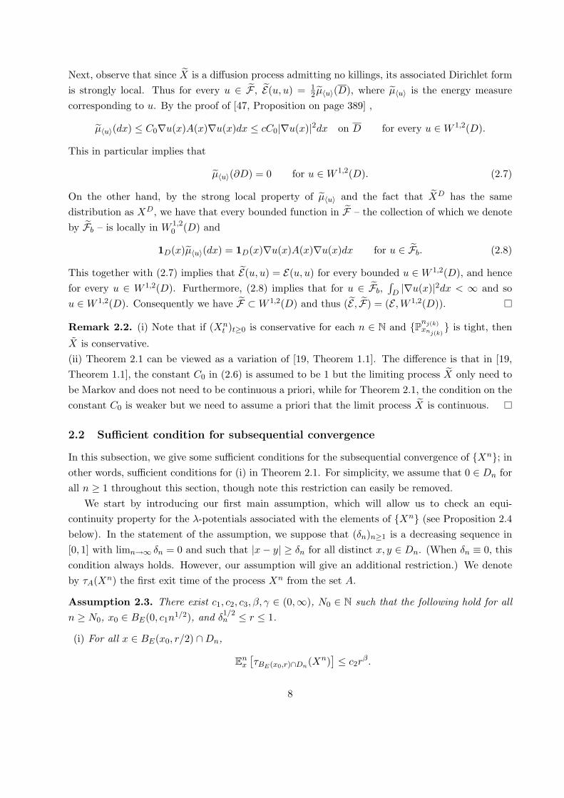
xyz

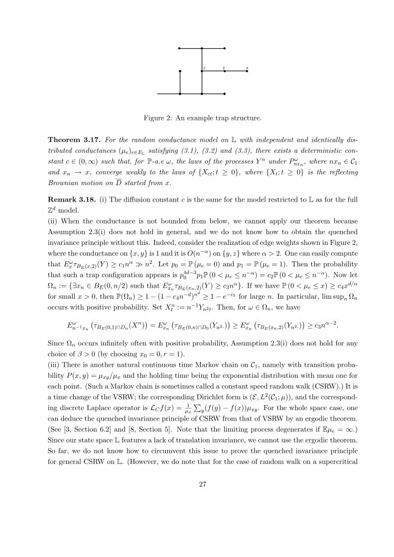
Figure 2: An example trap structure.

Theorem 3.17. For the random conductance model on L with independent and identically dis-tributed conductances (µe)e2EL satisfying (3.1), (3.2) and (3.3), there exists a deterministic con-stant c 2 (0,1) such that, for P-a.e !, the laws of the processes Y n under P!

nxn, where nxn 2 C1

and xn ! x, converge weakly to the laws of {Xct; t � 0}, where {Xt; t � 0} is the reflectingBrownian motion on D started from x.

Remark 3.18. (i) The di↵usion constant c is the same for the model restricted to L as for the fullZd model.(ii) When the conductance is not bounded from below, we cannot apply our theorem becauseAssumption 2.3(i) does not hold in general, and we do not know how to obtain the quenchedinvariance principle without this. Indeed, consider the realization of edge weights shown in Figure 2,where the conductance on {x, y} is 1 and it is O(n�↵) on {y, z} where ↵ > 2. One can easily computethat E!

x ⌧BE(x,2)(Y ) � c1n↵ � n2. Let p0 = P (µe = 0) and p1 = P (µe = 1). Then the probabilitythat such a trap configuration appears is p4d�3

0 p1P (0 < µe n�↵) = c2P (0 < µe n�↵). Now let⌦n := {9xn 2 BE(0, n/2) such that E!

xn⌧BE(xn,2)(Y ) � c3n↵}. If we have P (0 < µe x) � c4xd/↵

for small x > 0, then P(⌦n) � 1� (1� c4n�d)nd � 1� e�c5 for large n. In particular, lim supn⌦n

occurs with positive probability. Set Xnt := n�1Yn2t. Then, for ! 2 ⌦n, we have

E!n�1xn

�⌧BE(0,1)\Dn

(Xn)�

= E!xn

�⌧BE(0,n)\D0

(Yn2·)�� E!

xn

�⌧BE(xn,2)(Yn2·)

�� c3n

↵�2.

Since ⌦n occurs infinitely often with positive probability, Assumption 2.3(i) does not hold for anychoice of � > 0 (by choosing x0 = 0, r = 1).(iii) There is another natural continuous time Markov chain on C1, namely with transition proba-bility P (x, y) = µxy/µx and the holding time being the exponential distribution with mean one foreach point. (Such a Markov chain is sometimes called a constant speed random walk (CSRW).) It isa time change of the VSRW; the corresponding Dirichlet form is (E , L2(C1;µ)), and the correspond-ing discrete Laplace operator is LCf(x) = 1

µx

Py(f(y) � f(x))µxy. For the whole space case, one

can deduce the quenched invariance principle of CSRW from that of VSRW by an ergodic theorem.(See [3, Section 6.2] and [8, Section 5]. Note that the limiting process degenerates if Eµe = 1.)Since our state space L features a lack of translation invariance, we cannot use the ergodic theorem.So far, we do not know how to circumvent this issue to prove the quenched invariance principlefor general CSRW on L. (However, we do note that for the case of random walk on a supercritical

27

percolation cluster, the CSRW and VSRW behave similarly, and the quenched invariance principlefor the CSRW can be proved in a similar way as for the VSRW case. Moreover, the quenchedinvariance principle for the discrete time simple random walk on C1 follows easily from that for theCSRW.)(iv) To extend Theorem 3.17 to apply to more general domains, it will be enough to check thepercolation estimates from which we deduced Assumptions 2.3 and 2.6 in these settings. Whilstwe believe doing so should be possible, at least under certain smoothness assumptions on thedomain boundary, we do not feel the article would benefit significantly by the increased technicalcomplication of pursuing such results, and consequently omit to do so here. Instead we restrictour discussion of more general domains to the case of uniformly elliptic conductances, where therelevant estimates are straightforward to check (see Section 4.2 below). Similarly, given suitablefull space quenched invariance principles and percolation estimates (namely the estimates given inLemmas 3.1 – 3.3), our results should readily adapt to percolation models on other lattices.(v) Given the various estimates we have established so far, it is possible to extend the quenchedinvariance principle of Theorem 3.17 to a local limit theorem, i.e. a result describing the uniformconvergence of transition densities. More specifically, the additional ingredient needed for this is anequicontinuity result for the rescaled transition densities on C1, which can be obtained by applyingan argument similar to that used to deduce Assumption 2.3(ii), together with the heat kernelupper bound estimate of Proposition 3.11. Since the proof of such a result is relatively standard(cf. [9, 25]), we will only write out the details in the compact box case (see Section 4.1 below), whereconvergence of transition densities is also useful for establishing convergence of mixing times.

4 Other Examples

4.1 Random conductance model in a box

The purpose of this section is to explain how to adapt the results of Section 3 to the compact spacecase. For d � 2 fixed, set B(n) := [�n, n]d \ Zd, let EB(n) = {e = {x, y} : x, y 2 B(n), |x� y| = 1}be the set of nearest neighbor bonds, and suppose µ = (µe)e2EZd is a collection of independentrandom variables satisfying the assumptions made on the weights in Section 3, i.e. (3.1), (3.2) and(3.3). For each n and each realization of µ, let C1(n) be the largest component of B(n) that isconnected by edges satisfying µe > 0, and let Y n be the VSRW on C1(n). We will write P!

n,x forthe quenched law of Y n started from x 2 C1(n). The aim of this section is to show, via anotherapplication of Theorem 2.1, that Xn = (Xn

t )t�0, defined by setting

Xnt := n�1Y n

n2t,

converges as n !1 to reflecting Brownian motion on D = [�1, 1]d, for almost-every realization ofthe random environment µ. We observe that, in the case of uniformly elliptic random conductances,this result was recently established using an alternative argument in [18]. Note also that, by

28

in

Ci1(n)

C1(n)

C1(n) \ B"i (n)

= Ci1(n) \ B"

i (n)

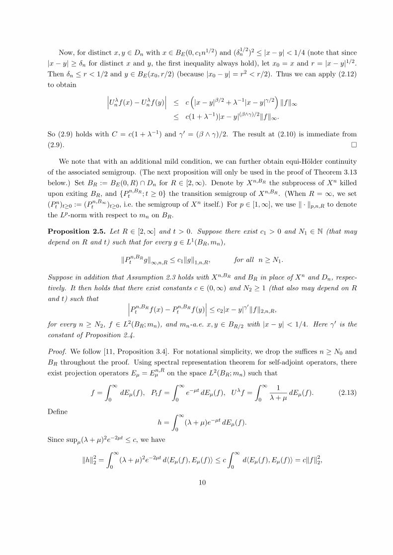
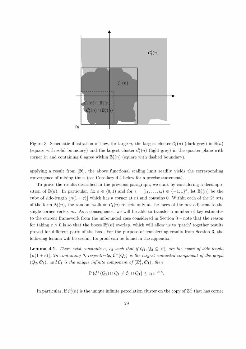
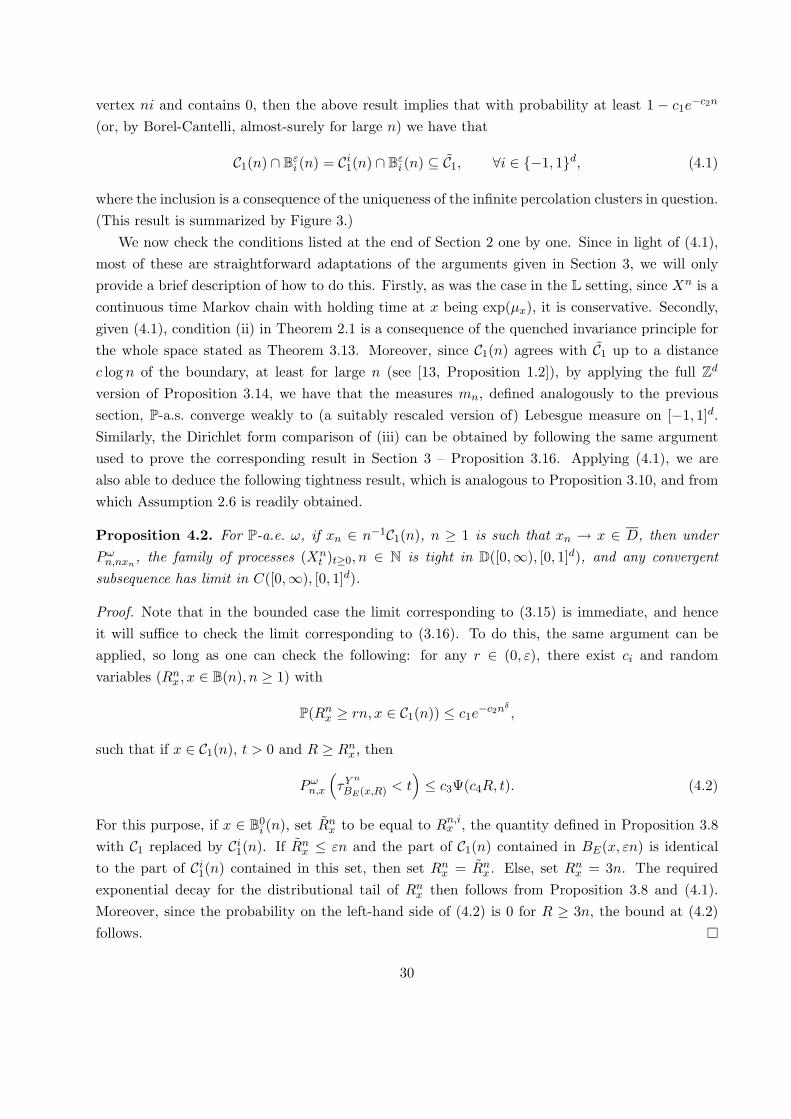
Figure 3: Schematic illustration of how, for large n, the largest cluster C1(n) (dark-grey) in B(n)(square with solid boundary) and the largest cluster Ci

1(n) (light-grey) in the quarter-plane withcorner in and containing 0 agree within B"

i (n) (square with dashed boundary).

applying a result from [26], the above functional scaling limit readily yields the correspondingconvergence of mixing times (see Corollary 4.4 below for a precise statement).

To prove the results described in the previous paragraph, we start by considering a decompo-sition of B(n). In particular, fix " 2 (0, 1) and for i = (i1, . . . , id) 2 {�1, 1}d, let B"

i (n) be thecube of side-length bn(1 + ")c which has a corner at ni and contains 0. Within each of the 2d setsof the form B"

i (n), the random walk on C1(n) reflects only at the faces of the box adjacent to thesingle corner vertex ni. As a consequence, we will be able to transfer a number of key estimatesto the current framework from the unbounded case considered in Section 3 – note that the reasonfor taking " > 0 is so that the boxes B"

i (n) overlap, which will allow us to ‘patch’ together resultsproved for di↵erent parts of the box. For the purpose of transferring results from Section 3, thefollowing lemma will be useful. Its proof can be found in the appendix.

Lemma 4.1. There exist constants c1, c2 such that if Q1, Q2 ✓ Zd+ are the cubes of side length

bn(1 + ")c, 2n containing 0, respectively, C+(Q2) is the largest connected component of the graph(Q2,O1), and C1 is the unique infinite component of (Zd

+,O1), then

P�C+(Q2) \Q1 6= C1 \Q1

� c1e

�c2n.

In particular, if Ci1(n) is the unique infinite percolation cluster on the copy of Zd

+ that has corner

29

vertex ni and contains 0, then the above result implies that with probability at least 1 � c1e�c2n

(or, by Borel-Cantelli, almost-surely for large n) we have that

C1(n) \ B"i (n) = Ci

1(n) \ B"i (n) ✓ C1, 8i 2 {�1, 1}d, (4.1)

where the inclusion is a consequence of the uniqueness of the infinite percolation clusters in question.(This result is summarized by Figure 3.)

We now check the conditions listed at the end of Section 2 one by one. Since in light of (4.1),most of these are straightforward adaptations of the arguments given in Section 3, we will onlyprovide a brief description of how to do this. Firstly, as was the case in the L setting, since Xn is acontinuous time Markov chain with holding time at x being exp(µx), it is conservative. Secondly,given (4.1), condition (ii) in Theorem 2.1 is a consequence of the quenched invariance principle forthe whole space stated as Theorem 3.13. Moreover, since C1(n) agrees with C1 up to a distancec log n of the boundary, at least for large n (see [13, Proposition 1.2]), by applying the full Zd

version of Proposition 3.14, we have that the measures mn, defined analogously to the previoussection, P-a.s. converge weakly to (a suitably rescaled version of) Lebesgue measure on [�1, 1]d.Similarly, the Dirichlet form comparison of (iii) can be obtained by following the same argumentused to prove the corresponding result in Section 3 – Proposition 3.16. Applying (4.1), we arealso able to deduce the following tightness result, which is analogous to Proposition 3.10, and fromwhich Assumption 2.6 is readily obtained.

Proposition 4.2. For P-a.e. !, if xn 2 n�1C1(n), n � 1 is such that xn ! x 2 D, then underP!

n,nxn, the family of processes (Xn

t )t�0, n 2 N is tight in D([0,1), [0, 1]d), and any convergentsubsequence has limit in C([0,1), [0, 1]d).

Proof. Note that in the bounded case the limit corresponding to (3.15) is immediate, and henceit will su�ce to check the limit corresponding to (3.16). To do this, the same argument can beapplied, so long as one can check the following: for any r 2 (0, "), there exist ci and randomvariables (Rn

x , x 2 B(n), n � 1) with

P(Rnx � rn, x 2 C1(n)) c1e

�c2n�,

such that if x 2 C1(n), t > 0 and R � Rnx , then

P!n,x

⇣⌧Y n

BE(x,R) < t⌘ c3 (c4R, t). (4.2)

For this purpose, if x 2 B0i (n), set Rn

x to be equal to Rn,ix , the quantity defined in Proposition 3.8

with C1 replaced by Ci1(n). If Rn

x "n and the part of C1(n) contained in BE(x, "n) is identicalto the part of Ci

1(n) contained in this set, then set Rnx = Rn

x . Else, set Rnx = 3n. The required

exponential decay for the distributional tail of Rnx then follows from Proposition 3.8 and (4.1).

Moreover, since the probability on the left-hand side of (4.2) is 0 for R � 3n, the bound at (4.2)follows.

30

It remains to check Assumption 2.3. For part (i), we simply note that the combination of (3.19)(or more precisely, the exponential tail bound for N0 that appears as (3.21)) and (4.1) in a standardBorel-Cantelli argument implies the following: there exist c⇤, c1 > 0 (non-random) and N0(!) suchthat if n � N0(!), then, for each x0, x 2 n�1C1(n) and c⇤/n1/2 r0 1,

E!n,x

�⌧BE(x0,r0)(Xn)

� c1r

02,

as desired. For part (ii) of this assumption, first note that we can obtain the elliptic Har-nack inequality uniformly for Xn-harmonic functions on BE(x0, R), where x0 2 n�1C1(n) and(logn)2/�/n R 1 for large n. (This can be proved similarly as before, namely when x0 2 B0

i (n),Theorem 3.12 can be applied by replacing C1 by Ci

1(n) due to (4.1).) Given the elliptic Harnackinequality, we can obtain Holder continuity in a similar way as in the proof of [9, Proposition 3.2],for example. Hence we have established the following.

Theorem 4.3. There exists a constant c 2 (0,1) such that, for P-a.e. !, the process Xn underP!

n,nxn, where nxn 2 C1 and xn ! x 2 [�1, 1]d, converges in distribution to (Bct)t�0, where (Bt)t�0

is the reflecting Brownian motion on [�1, 1]d started from x.

Next, for p 2 [1,1], define the Lp mixing time of the VSRW on C1(n) to be

tpmix(C1(n)) := inf

8<:t > 0 : sup

x2C1(n)

ZC1(n)

|qnt (x, y)� 1|p ⇡n(dy)

!1/p

<14

9=; , (4.3)

where we denote by qn the transition density of the VSRW with respect to its (unique) invariantprobability measure ⇡n. The above result then has the following corollary. Note that in thepercolation setting, the obvious adaptation of this result to discrete time gives a refinement of thefirst statement of [13, Theorem 1.1].

Corollary 4.4. Fix p 2 [1,1]. For P-a.e. !, we have that

n�2tpmix(C1(n)) ! c�1tpmix([�1, 1]d),

where c is the constant of Theorem 4.3, and tpmix([�1, 1]d) is the mixing time of reflecting Brownianmotion on [�1, 1]d (defined analogously to (4.3)).

Proof. First note that a simple rescaling yields that, P-a.s., ⇡n converges weakly to a rescaled versionof Lebesgue measure on [�1, 1]d. The P-a.s. Hausdor↵ convergence of n�1C1(n) (equipped withEuclidean distance) to [�1, 1]d is a straightforward consequence of this. To establish the corollaryby applying [26, Theorem 1.4], it will thus be enough to extend the weak convergence result ofTheorem 4.3 to a uniform convergence of transition densities (so as to satisfy [26, Assumption 1]).According to [26, Proposition 2.4] (cf. [25, Theorem 15]) and the quenched invariance principlementioned above, it is enough to show [26, (2.11)], namely, for any 0 < a < b < 1,

lim�!0

lim supn!1

supx,y,z2n�1C1(n):dE(ny,nz)n�

supt2[a,b]

��qnn2t(nx, ny)� qn

n2t(nx, nz)�� = 0. (4.4)

31

To prove this, first we have the following Holder continuity, which can be checked similarly toAssumption 2.3(ii):

��qnn2t(nx, ny)� qn

n2t(nx, nz)�� c1|y � z|�kqn

n2t(nx, ·)k1, 8x, y, z 2 n�1C1(n). (4.5)

For 0 < a t < 1, say, a compact version of Proposition 3.11 and scaling gives that

kqnn2t(nx, ·)k1 c3|C1(n)|(n2t)�d/2 c3a

�d/2

for large n. For t � 1, Cauchy-Schwarz and monotonicity of qnn2t(nx, nx) implies kqn

n2t(nx, ·)k1 c4.In particular,

kqnn2t(nx, ·)k1 c2(a) (4.6)

uniformly in x 2 Dn, t � a, for large n, P-a.s. Thus, for t 2 [a, b], the right-hand side of (4.5) isbounded from above by c3(a)|y � z|� . Taking n !1 and then � ! 0, we obtain (4.4).

Finally, as a corollary of the heat kernel continuity derived in the proof of the previous result,we obtain the following local central limit theorem. We let gn : [�1, 1]d ! C1(n) be such that gn(x)is a closest point in C1(n) to nx in the | · |1-norm. (If there is more than one such point, we chooseone arbitrarily.)

Corollary 4.5. Let qt(·, ·) be the heat kernel of the reflecting Brownian motion on [�1, 1]d. ForP-a.e. ! and for any 0 < a < b < 1, we have that

limn!1

supx,y2[�1,1]d

supt2[a,b]

|qnnt(gn(x), gn(y))� qct(x, y)| = 0, (4.7)

where c is the constant of Theorem 4.3.

Proof. Given the above results, the proof is standard. By (4.5) and (4.6) and the Ascoli-Arzelatheorem (along with the Hausdor↵ convergence of n�1C1(n) to [�1, 1]d), there exists a subsequenceof qn

nt(gn(·), gn(·)) that converges uniformly to a jointly continuous function on [a, b] ⇥ [�1, 1]d ⇥[�1, 1]d. Using Theorem 4.3, it can be checked that this function is the heat kernel of the limitingprocess. Since the limiting process is unique, we have the convergence of the full sequence ofqnnt(gn(·), gn(·)). The uniform convergence in (4.7) is then another consequence of (4.5) and (4.6).

4.2 Uniformly elliptic random conductances in uniform domains

When the conductances are uniform elliptic, i.e. bounded from above and below by fixed positiveconstants, we can obtain quenched invariance principles for a much wider class of domains thanthose considered in the examples presented so far. In particular, let D be a uniform domain inRd, d � 2. For each n � 1, let Dn be the largest connected component of of nD \ Zd, and set

32

EDn= {e = {x, y} : x, y 2 Dn, |x� y| = 1}. Suppose µ = (µe)e2EZd is a collection of independent

random variables such that

P(C1 µe C2) = 1, 8e 2 EZd ,

where C1, C2 are non-random positive constants. Let Y n be either VSRW or CSRW on Dn. More-over, set Dn := n�1Dn and define Xn

t := n�1Y nn2t. It is then the case that Xn = (Xn

t )t�0 convergesas n ! 1 to a (constant time change of) reflecting Brownian motion on D, for P-almost-everyrealization of the random environment µ.

Since checking the details for this case is much simpler than for previous settings, we will notprovide a full proof of the result described in the previous paragraph, but merely indicate how toestablish the key estimates. Indeed, in the uniformly elliptic case, we have

c1Rd n�d |BE(x,R) \Dn| c2R

d, c3Rd n�dµ(BE(x, nR) \ Dn) c4R

d

for all large n and all n�1 R diam (D), x 2 D, where ci are non-random positive constants.Furthermore, the weak Poincare inequality (3.10) holds both for the counting measure and n�dµ

uniformly for n�1 R diam (D), in the sense that the constants do not depend on n. Giventhese, we can apply [28] (and the natural relations between heat kernels of discrete and continuoustime Markov chains) to deduce

c5t�d/2 exp(�c6|x� y|2/t) qn

t (x, y) c7t�d/2 exp(�c8|x� y|2/t), |x� y| t diam (D),

where qnt (x, y) is defined as n�dP!

x (Xnt = y) for the VSRW and n�dµ(ny)�1P!

x (Xnt = y) for the

CSRW. Given these heat kernel estimates, it is then straightforward to verify the conditions requiredfor the quenched invariance principle by applying similar arguments to those of Sections 3 and 4.1.

4.3 Uniform elliptic random divergence form in domains

In this section, we explain how Theorem 2.1 can be applied in the random divergence form setting.Let D be a uniform domain in Rd, d � 2. Assume that we have a random divergence form asfollows. There exists a probability space (⌦, P) with shift operators (⌧x)x2Rd that are ergodic, anda symmetric d⇥ d matrix A!(x) for each x 2 Rd and ! 2 ⌦ such that A!(x) = A⌧x!(0) and

P(c1I A!(x) c2I) = 1, 8x 2 Rd,

where c1, c2 2 (0,1) are deterministic constants. For n � 1, let

En(f, f) =12

ZnDrf(x)A!(x)rf(x)dx.

Let (Y nt )t�0 be the reflected di↵usion process on nD associated with the regular Dirichlet form

(En,W 1,2(nD)) on L2(nD; dx), and set Xnt := n�1Y n

n2t. (A natural setting would be to take D tobe a cone. In this case nD = D, so the random di↵usion matrix A!(x) only needs to be defined

33

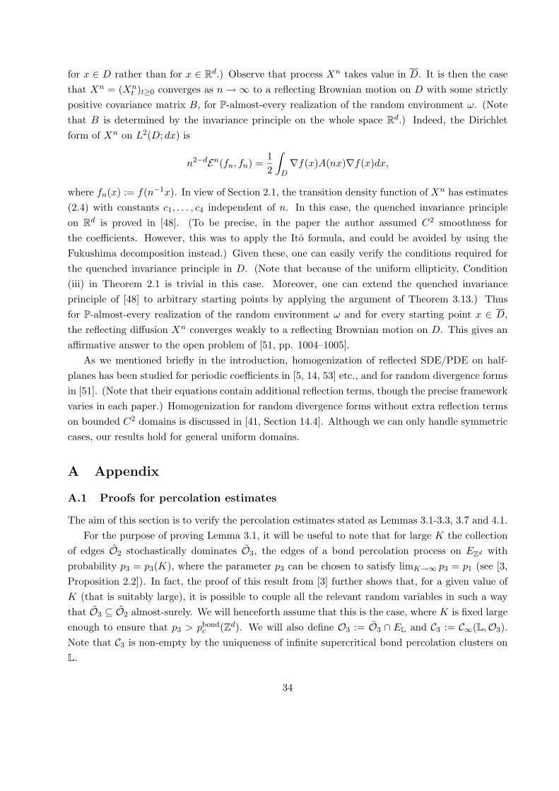
for x 2 D rather than for x 2 Rd.) Observe that process Xn takes value in D. It is then the casethat Xn = (Xn

t )t�0 converges as n !1 to a reflecting Brownian motion on D with some strictlypositive covariance matrix B, for P-almost-every realization of the random environment !. (Notethat B is determined by the invariance principle on the whole space Rd.) Indeed, the Dirichletform of Xn on L2(D; dx) is

n2�dEn(fn, fn) =12

ZDrf(x)A(nx)rf(x)dx,

where fn(x) := f(n�1x). In view of Section 2.1, the transition density function of Xn has estimates(2.4) with constants c1, . . . , c4 independent of n. In this case, the quenched invariance principleon Rd is proved in [48]. (To be precise, in the paper the author assumed C2 smoothness forthe coe�cients. However, this was to apply the Ito formula, and could be avoided by using theFukushima decomposition instead.) Given these, one can easily verify the conditions required forthe quenched invariance principle in D. (Note that because of the uniform ellipticity, Condition(iii) in Theorem 2.1 is trivial in this case. Moreover, one can extend the quenched invarianceprinciple of [48] to arbitrary starting points by applying the argument of Theorem 3.13.) Thusfor P-almost-every realization of the random environment ! and for every starting point x 2 D,the reflecting di↵usion Xn converges weakly to a reflecting Brownian motion on D. This gives ana�rmative answer to the open problem of [51, pp. 1004–1005].

As we mentioned briefly in the introduction, homogenization of reflected SDE/PDE on half-planes has been studied for periodic coe�cients in [5, 14, 53] etc., and for random divergence formsin [51]. (Note that their equations contain additional reflection terms, though the precise frameworkvaries in each paper.) Homogenization for random divergence forms without extra reflection termson bounded C2 domains is discussed in [41, Section 14.4]. Although we can only handle symmetriccases, our results hold for general uniform domains.

A Appendix

A.1 Proofs for percolation estimates

The aim of this section is to verify the percolation estimates stated as Lemmas 3.1-3.3, 3.7 and 4.1.For the purpose of proving Lemma 3.1, it will be useful to note that for large K the collection

of edges O2 stochastically dominates O3, the edges of a bond percolation process on EZd withprobability p3 = p3(K), where the parameter p3 can be chosen to satisfy limK!1 p3 = p1 (see [3,Proposition 2.2]). In fact, the proof of this result from [3] further shows that, for a given value ofK (that is suitably large), it is possible to couple all the relevant random variables in such a waythat O3 ✓ O2 almost-surely. We will henceforth assume that this is the case, where K is fixed largeenough to ensure that p3 > pbond

c (Zd). We will also define O3 := O3 \ EL and C3 := C1(L,O3).Note that C3 is non-empty by the uniqueness of infinite supercritical bond percolation clusters onL.

34

Proof of Lemma 3.1. First observe that O3 ✓ O2 ✓ O1. It follows that there exists an infiniteconnected component C of (L,O2) such that C3 ✓ C ✓ C1. For such a C (at the moment, we do notknow its uniqueness), we have that C1\C ✓ H3 ✓ L\C3. Denote by G(x) the connected componentof L\C3 containing x (if x 2 C3, we set G(x) = ;). To prove part (i) of the lemma, it su�ce to showthat there exist constants c1, c2 such that: for each x 2 L,

P (diam(G(x)) � n) c1e�c2n. (A.1)

For this, we will follow the renormalization argument used in the proof of [17, Proposition 2.3],making the adaptations necessary to deal with the boundary issues that arise in our setting.

We start by coupling a finite range-dependent site percolation model with our bond percolationprocess. For L 2 N, x 2 Zd, define

QL(x) := L(x + e1 + · · ·+ ed1) + [0, L]d \ Zd, Q3L(x) := L(x + e1 + · · ·+ ed1) + [�L, 2L]d \ Zd,

where e1, . . . , ed are the standard basis vectors for Zd. Given these sets, let GL(x) be the eventsuch that

• there exists an O3-crossing cluster for QL(x) in Q3L(x), i.e. there is a O3-connected clusterin Q3L(x) that, for all d directions, joins the ‘left face’ to the ‘right face’ of QL(x),

• all paths along edges of O3 that are contained in Q3L(x) and have diameter greater than L

are connected to the (necessarily unique) crossing cluster.

We will say that x 2 Zd is ‘white’ if GL(x) holds and ‘black’ otherwise, and make the importantobservation that if two neighboring vertices are white, then their crossing clusters must be con-nected. Since p3 > pbond

c (Zd), we can apply (the bond percolation version of) [49, Theorem 5] ford = 2 and [50, Theorem 3.1] for d � 3 to deduce that

limL!1

P (GL(x)) = 1, (A.2)

(cf. [4, (2.24)]). Moreover, although (1GL(x))x2Zd are not independent, the dependence betweenthese random variables is of finite range. Thus, by [44, Theorem 0.0], one can suppose that, forsuitably large L, the collection (1GL(x))x2Zd dominates a site percolation process on Zd of densityarbitrarily close to 1. Noting that for any infinite connected graph G with maximal vertex degree� the critical site and bond percolation probabilities satisfy

psitec (G) 1� (1� pbond

c (G))��1,

([34, Theorem 3]), we have that psitec (L) is bounded above by 1� (1� pbond

c (Zd))2d�1 < 1. Hence,by taking L suitably large, it is possible to assume that there is a non-zero probability of 0 beingcontained in an infinite cluster of white vertices in L. From this result, a standard ergodicityargument with respect to the shift x 7! x + e1 + · · · + ed1 allows one to check that, P-a.s., there

35

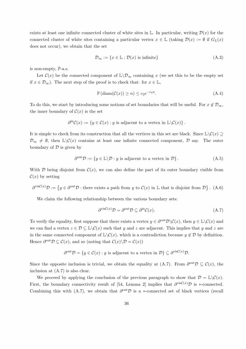
exists at least one infinite connected cluster of white sites in L. In particular, writing D(x) for theconnected cluster of white sites containing a particular vertex x 2 L (taking D(x) := ; if GL(x)does not occur), we obtain that the set

D1 := {x 2 L : D(x) is infinite} (A.3)

is non-empty, P-a.s.Let C(x) be the connected component of L\D1 containing x (we set this to be the empty set

if x 2 D1). The next step of the proof is to check that: for x 2 L,

P (diam(C(x)) � n) c3e�c4n. (A.4)

To do this, we start by introducing some notions of set boundaries that will be useful. For x 62 D1,the inner boundary of C(x) is the set

@inC(x) := {y 2 C(x) : y is adjacent to a vertex in L\C(x)} .

It is simple to check from its construction that all the vertices in this set are black. Since L\C(x) ◆D1 6= ;, then L\C(x) contains at least one infinite connected component, D say. The outerboundary of D is given by

@outD := {y 2 L\D : y is adjacent to a vertex in D} . (A.5)

With D being disjoint from C(x), we can also define the part of its outer boundary visible fromC(x) by setting

@visC(x)D :=�y 2 @outD : there exists a path from y to C(x) in L that is disjoint from D

. (A.6)

We claim the following relationship between the various boundary sets:

@visC(x)D = @outD ✓ @inC(x). (A.7)

To verify the equality, first suppose that there exists a vertex y 2 @outD\C(x), then y 2 L\C(x) andwe can find a vertex z 2 D ✓ L\C(x) such that y and z are adjacent. This implies that y and z arein the same connected component of L\C(x), which is a contradiction because y 62 D by definition.Hence @outD ✓ C(x), and so (noting that C(x)\D = C(x))

@outD = {y 2 C(x) : y is adjacent to a vertex in D} ✓ @visC(x)D.

Since the opposite inclusion is trivial, we obtain the equality at (A.7). From @outD ✓ C(x), theinclusion at (A.7) is also clear.

We proceed by applying the conclusion of the previous paragraph to show that D = L\C(x).First, the boundary connectivity result of [54, Lemma 2] implies that @visC(x)D is ⇤-connected.Combining this with (A.7), we obtain that @outD is a ⇤-connected set of black vertices (recall

36

that the vertices of @inC(x) are black). Secondly, note that if Pp is the law of a parameter p sitepercolation process on Zd and C⇤ is the corresponding ⇤-connected component of closed verticescontaining 0, then for suitably large p we have that

Pp (C⇤ � n) c5e�c6n, (A.8)

(see [1, Theorem 7.3] and [2, Proposition 7.6]). In particular, it is easy to check from this that all⇤-connected components of closed vertices in the site percolation process with this choice of p arefinite, Pp-a.s. Hence, because (1GL(x))x2Zd dominates a site percolation process whose parametercan be made arbitrarily close to 1 by taking L suitably large, it must be the case that, for largeL, @outD is P-a.s. a finite set. Since D is infinite, it readily follows that L\D is also finite. Now,suppose D1 is a connected component of L\C(x) distinct from D and such that D1 \D1 6= ;. Bythe definition of D1, it holds that D1\D(y) 6= ; for some y such that D(y) is an infinite set. SinceD1 [ D(y) is an infinite connected component of L\C(x), it must be the case that D1 is infinite.However, this contradicts the finiteness of L\D, and so no such D1 can exist. Thus it must be thecase that if D1 is a connected component of L\C(x) distinct from D, then D1 \ D1 = ;. Since,similar to the results of the previous paragraph, we have that @outD1 ✓ @inC(x), the set D1 [ C(x)must be a connected component of L\D1. By the definition of C(x), this implies that D1 = ;,which yields D = L\C(x) as required.

An immediate corollary of the equality D = L\C(x) is that @inC(x) = @outD, which, as we havealready established, is a finite ⇤-connected component of black vertices. We will use these resultsto finally prove (A.4). Note first that diam(C(x)) = diam(@inC(x)). Hence, writing @B(x,m) forthe vertices of L at an `1 distance m from x,

P (diam(C(x)) � n) 1X

m=0

P�diam(@inC(x)) � n, @inC(x) \ @B(x,m) 6= ;

�

1X

m=0

Xy2@B(x,m)

P (diam(C⇤(y)) � n _m) ,

where C⇤(y) is the ⇤-connected component of black vertices in Zd containing y. By again comparing(1GL(x))x2Zd to a site percolation process, it is possible to apply (A.8) to deduce that the tail ofthe probability in the above sum is bounded above by c5e�c6(n_m). The estimate at (A.4) follows.

We now return to the problem of deriving the estimate at (A.1). For x 2 Zd, define the setQ0

L(x) := L(x+e1 + · · ·+ed1)+ [0, L)d\Zd, so that (Q0L(x))x2Zd is a partition of Zd. For x 2 L, let

a(x) be the closest element of L, with respect to `1 distance, to the x0 2 Zd such that x 2 Q0L(x0).

(Only when x is within a distance L of the boundary of L does x0 6= a(x).) It is then easy to checkthat if diam(G(x)) � L, then

G(x) ✓ [x02C(a(x))Q3L(x0). (A.9)

(cf. [17, (3.7)]). In particular, this implies that, if diam(G(x)) � L, then it must be the case thatdiam(G(x)) 3Ldiam(C(a(x))). Consequently, (A.1) follows from (A.4), and thus the proof of part(i) is complete.

37

Given part (i), we observe

P⇣9x 2 [�n, n]d \ L : #H(x) � (log n)d+1

⌘

(2n + 1)d supx2L

P⇣x 2 C1, #H(x) � (log n)d+1

⌘

(2n + 1)d supx2L

P⇣x 2 C1, diam(H(x)) � (log n)(d+1)/d

⌘

(2n + 1)dc1e�c2(log n)(d+1)/d

.

Since this is summable in n, part (ii) follows by a Borel-Cantelli argument.

We now work towards the proof of Lemma 3.2.

Proof of Lemma 3.2. To establish the bound in (3.4), let us start by recalling/adapting some defi-nitions from the previous proof. In particular, for x 2 Zd, define QL(x) and Q3L(x) as in the proofof Lemma 3.1. Moreover, let GL(x) be defined similarly, but with O3 replaced by O1, and redefinex being ‘white’ to mean that this version of GL(x) holds (and say x is ‘black’ otherwise). Notethat the statement (A.2) remains true with this definition of GL(x), and the dependence betweenthe random variables (1GL(x))x2Zd is only finite range, and so we can suppose that it dominates adominates a site percolation process on Zd of density arbitrarily close to 1.

Now, fix x, y 2 L, and recall the definition of a(x) from the proof of Lemma 3.1. If n is the `1

distance between a(x) and a(y), then there exists a nearest neighbor path a0, . . . , an in L such thata0 = a(x) and an = a(y). We claim that if x and y are both contained in C1, then there exists apath from x to y along edges of O1 whose vertices all lie in

[ni=0 [b2C⇤(ai)

Q3L(b), (A.10)

where C⇤(a) := {a} if a is white, otherwise C⇤(a) := C⇤(a) [ @outC⇤(a), where C⇤(a) is the ⇤-connected component of black sites in L containing a (@outC⇤(a) is the outer boundary of C⇤(a),defined similarly to (A.5)). This is essentially [4, Proposition 3.1] rewritten for L instead of Zd. Theone slight issue with modifying the proof of this result to our situation is that, unlike the Zd case,the outer boundary in L of a finite connected cluster of vertices, C say, is no longer ⇤-connectedin general and so it is not possible to run around it in quite the same way. However, this problemis readily overcome by applying [54, Lemma 2], which implies that for each x 62 C, the part of theouter boundary of C that is visible from x, @vis(x)C (cf. (A.6)), is ⇤-connected. A simple estimateof the number of vertices in the set at (A.10) yields

d1(x, y) (3L + 1)dnX

i=0

#C⇤(ai) (3L + 1)dnX

i=0

⇣1 + 3d#C⇤(ai)

⌘.

(We take C⇤(a) := ; if a is white.) Clearly C⇤(a) ✓ C⇤(a), where C⇤(a) is the ⇤-connected componentof black sites in Zd containing a. Consequently, we obtain that

P (x, y 2 C1 and d1(x, y) � cR) P

(3L + 1)dnX

i=0

⇣1 + 3d#C⇤(ai)

⌘� cR

!.

38

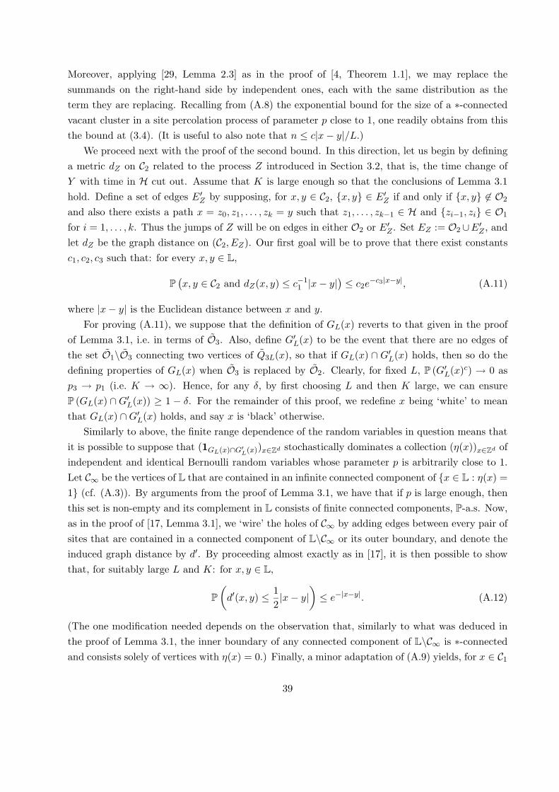
Moreover, applying [29, Lemma 2.3] as in the proof of [4, Theorem 1.1], we may replace thesummands on the right-hand side by independent ones, each with the same distribution as theterm they are replacing. Recalling from (A.8) the exponential bound for the size of a ⇤-connectedvacant cluster in a site percolation process of parameter p close to 1, one readily obtains from thisthe bound at (3.4). (It is useful to also note that n c|x� y|/L.)

We proceed next with the proof of the second bound. In this direction, let us begin by defininga metric dZ on C2 related to the process Z introduced in Section 3.2, that is, the time change ofY with time in H cut out. Assume that K is large enough so that the conclusions of Lemma 3.1hold. Define a set of edges E0

Z by supposing, for x, y 2 C2, {x, y} 2 E0Z if and only if {x, y} 62 O2

and also there exists a path x = z0, z1, . . . , zk = y such that z1, . . . , zk�1 2 H and {zi�1, zi} 2 O1

for i = 1, . . . , k. Thus the jumps of Z will be on edges in either O2 or E0Z . Set EZ := O2 [E0

Z , andlet dZ be the graph distance on (C2, EZ). Our first goal will be to prove that there exist constantsc1, c2, c3 such that: for every x, y 2 L,

P�x, y 2 C2 and dZ(x, y) c�1

1 |x� y|� c2e

�c3|x�y|, (A.11)

where |x� y| is the Euclidean distance between x and y.For proving (A.11), we suppose that the definition of GL(x) reverts to that given in the proof

of Lemma 3.1, i.e. in terms of O3. Also, define G0L(x) to be the event that there are no edges of

the set O1\O3 connecting two vertices of Q3L(x), so that if GL(x) \ G0L(x) holds, then so do the

defining properties of GL(x) when O3 is replaced by O2. Clearly, for fixed L, P (G0L(x)c) ! 0 as

p3 ! p1 (i.e. K ! 1). Hence, for any �, by first choosing L and then K large, we can ensureP (GL(x) \G0

L(x)) � 1 � �. For the remainder of this proof, we redefine x being ‘white’ to meanthat GL(x) \G0

L(x) holds, and say x is ‘black’ otherwise.Similarly to above, the finite range dependence of the random variables in question means that

it is possible to suppose that (1GL(x)\G0L(x))x2Zd stochastically dominates a collection (⌘(x))x2Zd ofindependent and identical Bernoulli random variables whose parameter p is arbitrarily close to 1.Let C1 be the vertices of L that are contained in an infinite connected component of {x 2 L : ⌘(x) =1} (cf. (A.3)). By arguments from the proof of Lemma 3.1, we have that if p is large enough, thenthis set is non-empty and its complement in L consists of finite connected components, P-a.s. Now,as in the proof of [17, Lemma 3.1], we ‘wire’ the holes of C1 by adding edges between every pair ofsites that are contained in a connected component of L\C1 or its outer boundary, and denote theinduced graph distance by d0. By proceeding almost exactly as in [17], it is then possible to showthat, for suitably large L and K: for x, y 2 L,

P✓

d0(x, y) 12|x� y|

◆ e�|x�y|. (A.12)

(The one modification needed depends on the observation that, similarly to what was deduced inthe proof of Lemma 3.1, the inner boundary of any connected component of L\C1 is ⇤-connectedand consists solely of vertices with ⌘(x) = 0.) Finally, a minor adaptation of (A.9) yields, for x 2 C1

39

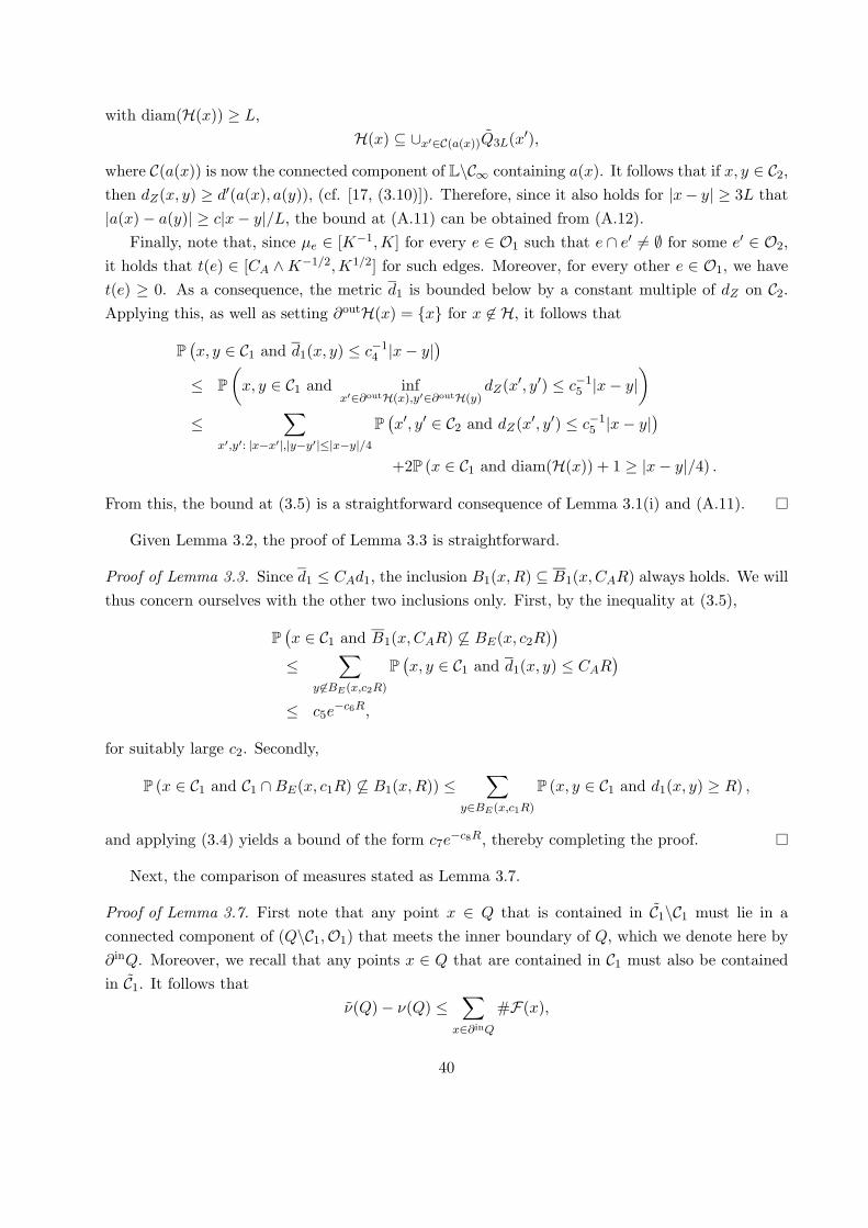
with diam(H(x)) � L,H(x) ✓ [x02C(a(x))Q3L(x0),

where C(a(x)) is now the connected component of L\C1 containing a(x). It follows that if x, y 2 C2,then dZ(x, y) � d0(a(x), a(y)), (cf. [17, (3.10)]). Therefore, since it also holds for |x� y| � 3L that|a(x)� a(y)| � c|x� y|/L, the bound at (A.11) can be obtained from (A.12).

Finally, note that, since µe 2 [K�1,K] for every e 2 O1 such that e \ e0 6= ; for some e0 2 O2,it holds that t(e) 2 [CA ^K�1/2,K1/2] for such edges. Moreover, for every other e 2 O1, we havet(e) � 0. As a consequence, the metric d1 is bounded below by a constant multiple of dZ on C2.Applying this, as well as setting @outH(x) = {x} for x 62 H, it follows that

P�x, y 2 C1 and d1(x, y) c�1

4 |x� y|�

P✓

x, y 2 C1 and infx02@outH(x),y02@outH(y)

dZ(x0, y0) c�15 |x� y|

◆

X

x0,y0: |x�x0|,|y�y0||x�y|/4

P�x0, y0 2 C2 and dZ(x0, y0) c�1

5 |x� y|�

+2P (x 2 C1 and diam(H(x)) + 1 � |x� y|/4) .

From this, the bound at (3.5) is a straightforward consequence of Lemma 3.1(i) and (A.11).

Given Lemma 3.2, the proof of Lemma 3.3 is straightforward.

Proof of Lemma 3.3. Since d1 CAd1, the inclusion B1(x,R) ✓ B1(x,CAR) always holds. We willthus concern ourselves with the other two inclusions only. First, by the inequality at (3.5),

P�x 2 C1 and B1(x,CAR) 6✓ BE(x, c2R)

�

Xy 62BE(x,c2R)

P�x, y 2 C1 and d1(x, y) CAR

�

c5e�c6R,

for suitably large c2. Secondly,

P (x 2 C1 and C1 \BE(x, c1R) 6✓ B1(x,R)) X

y2BE(x,c1R)

P (x, y 2 C1 and d1(x, y) � R) ,

and applying (3.4) yields a bound of the form c7e�c8R, thereby completing the proof.

Next, the comparison of measures stated as Lemma 3.7.

Proof of Lemma 3.7. First note that any point x 2 Q that is contained in C1\C1 must lie in aconnected component of (Q\C1,O1) that meets the inner boundary of Q, which we denote here by@inQ. Moreover, we recall that any points x 2 Q that are contained in C1 must also be containedin C1. It follows that

⌫(Q)� ⌫(Q) X

x2@inQ

#F(x),

40

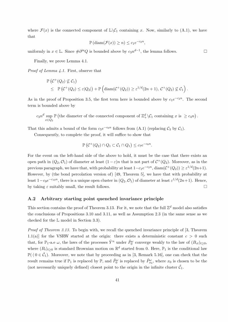
where F(x) is the connected component of L\C1 containing x. Now, similarly to (A.1), we havethat

P (diam(F(x)) � n) c1e�c2n,

uniformly in x 2 L. Since #@inQ is bounded above by c3nd�1, the lemma follows.

Finally, we prove Lemma 4.1.

Proof of Lemma 4.1. First, observe that

P�C+(Q2) 6✓ C1

� P

�C+(Q2) "|Q2|

�+ P

⇣diam(C+(Q2)) � "1/d(2n + 1), C+(Q2) 6✓ C1

⌘.

As in the proof of Proposition 3.5, the first term here is bounded above by c1e�c2n. The secondterm is bounded above by

c3nd sup

x2Q2

P�the diameter of the connected component of Zd

+\C1 containing x is � c4n�.

That this admits a bound of the form c5e�c6n follows from (A.1) (replacing C3 by C1).Consequently, to complete the proof, it will su�ce to show that

P�C+(Q2) \Q1 ⇢ C1 \Q1

� c7e

�c8n.

For the event on the left-hand side of the above to hold, it must be the case that there exists anopen path in (Q2,O1) of diameter at least (1� ")n that is not part of C+(Q2). Moreover, as in theprevious paragraph, we have that, with probability at least 1�c1e�c2n, diam(C+(Q2)) � "1/d(2n+1).However, by (the bond percolation version of) [49, Theorem 5], we have that with probability atleast 1�c9e�c10n, there is a unique open cluster in (Q2,O1) of diameter at least "1/d(2n+1). Hence,by taking " suitably small, the result follows.

A.2 Arbitrary starting point quenched invariance principle

This section contains the proof of Theorem 3.13. For it, we note that the full Zd model also satisfiesthe conclusions of Propositions 3.10 and 3.11, as well as Assumption 2.3 (in the same sense as wechecked for the L model in Section 3.3).

Proof of Theorem 3.13. To begin with, we recall the quenched invariance principle of [3, Theorem1.1(a)] for the VSRW started at the origin: there exists a deterministic constant c > 0 suchthat, for P1-a.e !, the laws of the processes Y n under P!

0 converge weakly to the law of (Bct)t�0,where (Bt)t�0 is standard Brownian motion on Rd started from 0. Here, P1 is the conditional lawP(·| 0 2 C1). Moreover, we note that by proceeding as in [3, Remark 5.16], one can check that theresult remains true if P1 is replaced by P, and P!

0 is replaced by P!x0

, where x0 is chosen to be the(not necessarily uniquely defined) closest point to the origin in the infinite cluster C1.

41

Given the above result, the argument of this paragraph applies for P-a.e. !. Fix x 2 Rd, " > 0,and define

⌧n := infn

t > 0 : Y nt 2 BE(x, ")

o,

⌧B := inf {t > 0 : Bct 2 BE(x, ")} .

A standard argument gives us that, jointly with the convergence of the previous paragraph, ⌧n

converges in distribution to ⌧B. Letting T > 0 be a deterministic constant, it follows that thelaws of the processes (Y n

⌧n+t)t�0 under P!x0

(·| ⌧n T ) converge weakly to the law of (Bc(⌧+t))t�0,started from 0 and conditional on ⌧ T . Consequently, the Markov property gives us that forevery bounded, continuous function f : C([0,1), Rd) ! R,Z

BE(x,")E!

nyf(Y n)P!x0

⇣Y n

⌧n 2 dy|⌧n T⌘!Z

BE(x,")EB

y f(Bc·)PB0

�Bc⌧B 2 dy|⌧B T

�, (A.13)

where BE(x, ") is the closure of BE(x, "), PBx is the law of the standard Brownian motion B started

from x, and EBx is the corresponding expectation. Furthermore, it is elementary to check for such

f that, as " ! 0, ZBE(x,")

EBy f(Bc·)PB

0

�Bc⌧B 2 dy|⌧B T

�! EB

x f(Bc·). (A.14)

Suppose that the following also holds for every sequence of starting points xn 2 n�1C1 such thatxn ! x, every finite collection of times 0 < t1 < t2 < · · · < tk and all bounded, continuous functionsfi : Rd ! R, i = 1, . . . , k,

lim"!0

lim supn!1

�����Z

BE(x,")E!

nyf(Y nt )P!

x0

⇣Y n

⌧n 2 dy|⌧n T⌘� E!

nxnf(Y n

t )

����� = 0, (A.15)

where Y nt := (Y n

t1 , Ynt2 , . . . , Y

ntk). Combining (A.13), (A.14) and (A.15) readily yields that the finite-

dimensional distributions of Y n (under P!nxn

) converge to those of Bc· (under PBx ). Moreover, from

the full plane version of Proposition 3.10, we have that the laws of Y n under P!nxn

are tight. Thesetwo facts yields the desired quenched invariance principle.

To complete the argument of the previous paragraph and the proof of the theorem, it remainsto check the limit at (A.15) holds (simultaneously over sequences of starting points xn ! x, timest = (t1, . . . , tk), and functions f) for P-a.e. !. In fact, using the independent increments propertyof Y n and some standard analysis, it will su�ce to check the result for k = 2 and for functions f

of the form f(Y nt1 , Y

nt2 ) = f1(Y n

t1 )f2(Y nt2 ). Writing the semigroup of Y n as Pn, we have for such a

function f that �����Z

BE(x,")E!

nyf(Y nt1 , Y

nt2 )P

!x0

⇣Y n

⌧n 2 dy|⌧n T⌘� E!

nxnf(Y n

t1 , Ynt2 )

�����=

�����Z

BE(x,")Pn

t1g(y)P!x0

⇣Y n

⌧n 2 dy|⌧n T⌘� Pn

t1g(xn)

����� sup

y2BE(x,")\n�1C1

���Pnt1g(y)� Pn

t1g(xn)��� , (A.16)

42

where g := f1 ⇥ (Pnt2�t1f2) (which is a bounded, continuous function). Take R > 2 with x 2

BE(0, R/2) \ n�1C1. For each � > 1, it holds that

Pnt g = Pn,B�R

t (g1B�R) + (Pnt � Pn,B�R

t )(g1B�R) + Pnt (g1Bc

�R),

where Bs := BE(0, s) \ n�1C1. We have

|(Pnt � Pn,B�R

t )(g1B�R)(z) + Pnt (g1Bc

�R)(z)| kgk1P z

!(⌧nB�R

t) + kgk1P z!(Y n

t 2 Bc�R)

2kgk1P z!(⌧n

B�R t).

So, setting Bx," := BE(x, ") \ n�1C1, for large n we have

supy2Bx,"

���Pnt1g(y)� Pn

t1g(xn)���

supy2Bx,"

���Pn,B�Rt1 (g1B�R)(y)� Pn,B�R

t1 (g1B�R)(xn)���+ 4kgk1 sup

z2Bx,2"

P z!(⌧n

B�R t)

=: I1 + 4kgk1I2.

Now let us note that Assumption 2.3 holds for Xn killed on exiting B�R when Dn is replaced byB�R (which can be verified similarly to the discussion in Section 3.3 for the L case; for this, it isuseful to note that the killing does not have any e↵ect since points in B�R/2 are suitably far awayfrom the boundary of B�R). Moreover, applying the scaling relation qn

t (x, y) = ndqYtn2(nx, ny), by

Proposition 3.11 (for the full Zd model) we have, kPn,B�Rt gk1,n,�R c1t�d/2kgk1,n,�R whenever we

also have tn2 � c2(supx2B�RRx_1_ supx,y2B�R

2d1(x, y))1/4, where Rx is defined as in Proposition3.11. Hence a simple Borel-Cantelli argument using the tail estimate of that proposition to controlsupx2B�R

Rx and Lemma 3.2 to control supx,y2B�R2d1(x, y) yields that the above bound holds true

for all large n, P-a.s. Hence, by applying Proposition 2.5, we have I1 Ct(2")�0kgk2,n,�R for allx 2 BR/2 and all large n, P-a.s. By applying the full Zd version of Proposition 3.14, i.e. the vagueconvergence of mn to a multiple of Lebesgue, it follows that for P-a.e. !: for t > 0, R > 2 and� > 1,

lim"!0

lim supn!1

supx2BR/2

I1 = 0.

For I2, we will apply the full Zd version of the exit time bound of Proposition 3.8. In particular,this result implies that for P-a.e. !: for t > 0, R > 2 and � > 1,

lim"!0

lim supn!1

supx2BR/2

I2 lim"!0

lim supn!1

c2 (c3(�R/2� 2")n, tn2) = c2e�c3�2R2/t.

(Note that a Borel-Cantelli argument that depends on the tail estimate for Rx of Proposition 3.8 ishidden in the inequality.) Letting � !1, this converges to 0. Thus, we deduce that for fixed R > 2and P-a.e.-! that: for every sequence of starting points xn 2 n�1C1 such that xn ! x 2 BE(0, R/2),for every 0 < t1 < t2, for every bounded, continuous f1, f2, the expression at (A.16) converges to 0as n !1 and then " ! 0. Since there is no problem in extending this result to allow any x 2 Rd,we have thus completed the proof of (A.15).

43

Acknowledgement. Parts of this work were completed during visits by the first and secondnamed authors to the Research Institute for Mathematical Sciences, Kyoto University in early 2012and early 2013, respectively. Both authors kindly thank RIMS for the hospitality and financialsupport.

References

[1] Aizenman, M. and Barsky, D. J. (1987). Sharpness of the phase transition in percolation models. Comm.Math. Phys. 108 489–526.

[2] Aizenman, M. and Newman, C. M. (1984). Tree graph inequalities and critical behavior in percolationmodels. J. Statist. Phys. 36 107–143.

[3] Andres, S., Barlow, M. T., Deuschel, J.-D. and Hambly, B. M. (2013). Invariance principle for therandom conductance model. Probab. Theory Related Fields 156 535–580.

[4] Antal, P. and Pisztora, A. (1996). On the chemical distance for supercritical Bernoulli percolation. Ann.Probab. 24 1036–1048.

[5] Barles, G., Da Lio, F., Lions, P.-L. and Souganidis, P. E. (2008). Ergodic problems and periodichomogenization for fully non-linear equations in half-space type domains with Neumann boundaryconditions. Indiana Univ. Math. J. 57 2355–2376.

[6] Barlow, M. T. (2004). Random walks on supercritical percolation clusters. Ann. Probab. 32 3024–3084.

[7] Barlow, M. T. and Bass, R. F. (1989). The construction of Brownian motion on the Sierpinski carpet.Ann. Inst. H. Poincare Probab. Statist. 25 225–257.

[8] Barlow, M. T. and Deuschel, J.-D. (2010). Invariance principle for the random conductance model withunbounded conductances. Ann. Probab. 38 234–276.

[9] Barlow, M. T. and Hambly, B. M. (2009). Parabolic Harnack inequality and local limit theorem forpercolation clusters. Electron. J. Probab. 14 1–27.

[10] Barsky, D. J., Grimmett, G. R. and Newman, C. M. (1991). Percolation in half-spaces: equality ofcritical densities and continuity of the percolation probability. Probab. Theory Related Fields 90 111–148.

[11] Bass, R. F., Kassmann, M. and Kumagai, T. (2010). Symmetric jump processes: localization, heatkernels and convergence. Ann. Inst. Henri Poincare Probab. Stat. 46. 59–71.

[12] Benjamini, I., Chen, Z.-Q. and Rohde, S. (2004). Boundary trace of reflecting Brownian motions.Probab. Theory Related Fields 129 1-17.

[13] Benjamini, I. and Mossel, E. (2003). On the mixing time of a simple random walk on the super criticalpercolation cluster. Probab. Theory Related Fields 125 408–420.

[14] Bensoussan, A.,Lions, J. L. and Papanicolaou, G. (1978). Asymptotic methods in periodic media. Ed.North Holland, 1978.

44

[15] Berger, N. and Biskup, M. (2007). Quenched invariance principle for simple random walk on percolationclusters. Probab. Theory Related Fields 137 83–120.

[16] Biskup, M. (2011). Recent progress on the random conductance model. Probab. Surv. 8 294–373.

[17] Biskup, M. and Prescott, T. M. (2007). Functional CLT for random walk among bounded randomconductances. Electron. J. Probab. 12 1323–1348.

[18] Buckley, S. and Hambly, B. M. An invariance principle for random walk in a box in the randomconductance model. In preparation.

[19] Burdzy, K. and Chen, Z.-Q. (2008). Discrete approximations to reflected Brownian motion. Ann. Probab.36 698-727.

[20] Burdzy, K. and Chen, Z.-Q. (2013). Reflecting random walk in fractal domains. Ann. Probab. 41 2791–2819.

[21] Chen, Z.-Q. (1993). On reflecting di↵usion processes and Skorokhod decompositions. Probab. TheoryRelated Fields 94 281-316.

[22] Chen, Z.-Q. (1996). Reflecting Brownian motions and a deletion result for Sobolev spaces of order (1;2). Potential Analysis 5 383-401.

[23] Chen, Z.-Q. and Fukushima, M. (2012). Symmetric Markov Processes, Time Change, and BoundaryTheory. Princeton University Press.

[24] Chung, K. L. and Walsh, J. B. (2005). Markov Processes, Brownian Motion, and Time Symmetry,Second Edition. Springer.

[25] Croydon, D. A. and Hambly, B. M. (2008). Local limit theorems for sequences of simple random walkson graphs. Potential Anal. 29 351–389.

[26] Croydon, D. A., Hambly, B. M. and Kumagai, T. (2012). Convergence of mixing times for sequences ofrandom walks on finite graphs. Electron. J. Probab. 17 no. 3, 1-32.

[27] De Masi,A., Ferrari, P. A., Goldstein, S. and Wick, W. D. (1989). An invariance principle for reversibleMarkov processes. Applications to random motions in random environments. J. Statist. Phys. 55 787–855.

[28] Delmotte, T. (1999). Parabolic Harnack inequality and estimates of Markov chains on graphs. Rev.Mat. Iberoamericana 15. 181–232.

[29] Deuschel, J.-D. and Pisztora, A. (1996). Surface order large deviations for high-density percolation.Probab. Theory Related Fields 104 467–482.

[30] Durrett, R. (1996). Probability: theory and examples, second ed., Duxbury Press, Belmont, CA.

[31] Ethier, S. N. and Kurtz, T. G. (1986). Markov processes, Characterization and convergence, Wiley Seriesin Probability and Mathematical Statistics: Probability and Mathematical Statistics, John Wiley &Sons Inc., New York.

45

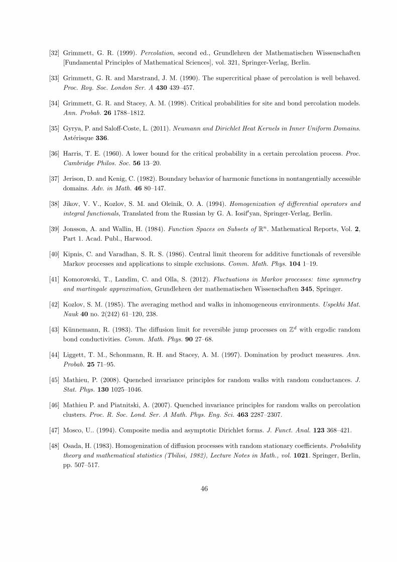
[32] Grimmett, G. R. (1999). Percolation, second ed., Grundlehren der Mathematischen Wissenschaften[Fundamental Principles of Mathematical Sciences], vol. 321, Springer-Verlag, Berlin.

[33] Grimmett, G. R. and Marstrand, J. M. (1990). The supercritical phase of percolation is well behaved.Proc. Roy. Soc. London Ser. A 430 439–457.

[34] Grimmett, G. R. and Stacey, A. M. (1998). Critical probabilities for site and bond percolation models.Ann. Probab. 26 1788–1812.

[35] Gyrya, P. and Salo↵-Coste, L. (2011). Neumann and Dirichlet Heat Kernels in Inner Uniform Domains.Asterisque 336.

[36] Harris, T. E. (1960). A lower bound for the critical probability in a certain percolation process. Proc.Cambridge Philos. Soc. 56 13–20.

[37] Jerison, D. and Kenig, C. (1982). Boundary behavior of harmonic functions in nontangentially accessibledomains. Adv. in Math. 46 80–147.

[38] Jikov, V. V., Kozlov, S. M. and Oleınik, O. A. (1994). Homogenization of di↵erential operators andintegral functionals, Translated from the Russian by G. A. Iosif0yan, Springer-Verlag, Berlin.

[39] Jonsson, A. and Wallin, H. (1984). Function Spaces on Subsets of Rn. Mathematical Reports, Vol. 2,Part 1. Acad. Publ., Harwood.

[40] Kipnis, C. and Varadhan, S. R. S. (1986). Central limit theorem for additive functionals of reversibleMarkov processes and applications to simple exclusions. Comm. Math. Phys. 104 1–19.

[41] Komorowski, T., Landim, C. and Olla, S. (2012). Fluctuations in Markov processes: time symmetryand martingale approximation, Grundlehren der mathematischen Wissenschaften 345, Springer.

[42] Kozlov, S. M. (1985). The averaging method and walks in inhomogeneous environments. Uspekhi Mat.Nauk 40 no. 2(242) 61–120, 238.

[43] Kunnemann, R. (1983). The di↵usion limit for reversible jump processes on Zd with ergodic randombond conductivities. Comm. Math. Phys. 90 27–68.

[44] Liggett, T. M., Schonmann, R. H. and Stacey, A. M. (1997). Domination by product measures. Ann.Probab. 25 71–95.

[45] Mathieu, P. (2008). Quenched invariance principles for random walks with random conductances. J.Stat. Phys. 130 1025–1046.

[46] Mathieu P. and Piatnitski, A. (2007). Quenched invariance principles for random walks on percolationclusters. Proc. R. Soc. Lond. Ser. A Math. Phys. Eng. Sci. 463 2287–2307.

[47] Mosco, U.. (1994). Composite media and asymptotic Dirichlet forms. J. Funct. Anal. 123 368–421.

[48] Osada, H. (1983). Homogenization of di↵usion processes with random stationary coe�cients. Probabilitytheory and mathematical statistics (Tbilisi, 1982), Lecture Notes in Math., vol. 1021. Springer, Berlin,pp. 507–517.

46

[49] Penrose, M. D. and Pisztora, A. (1996). Large deviations for discrete and continuous percolation. Adv.in Appl. Probab. 28 29–52.

[50] Pisztora, A. (1996). Surface order large deviations for Ising, Potts and percolation models. Probab.Theory Related Fields 104 427–466.

[51] Rhodes, R. (2010). Stochastic homogenization of reflected stochastic di↵erential equations. Electron. J.Probab. 15, Paper no. 31, 989–1023.

[52] Sidoravicius V. and Sznitman, A.-S. (2004). Quenched invariance principles for walks on clusters ofpercolation or among random conductances. Probab. Theory Related Fields 129 219–244.

[53] Tanaka, H. (1984). Homogenization of di↵usion processes with boundary conditions. Stoc. Anal. Appl.,Adv. Probab. Related Topics 7, Dekker, New York, 411–437.

[54] Timar, A. (2013). Boundary-connectivity via graph theory. Proc. Amer. Math. Soc. 141 475–480.

[55] Vaisala, J. (1988). Uniform domains. Tohoku Math. J. 40 101-118.

Zhen-Qing ChenDepartment of Mathematics, University of Washington, Seattle, WA 98195, USA.E-mail: zqchen@uw.edu

David A. CroydonDepartment of Statistics, University of Warwick, Coventry, CV4 7AL, United Kingdom.E-mail: d.a.croydon@warwick.ac.uk

Takashi KumagaiResearch Institute for Mathematical Sciences, Kyoto University, Kyoto 606-8502, Japan.E-mail: kumagai@kurims.kyoto-u.ac.jp

47