quantum optical experiments towards atom-photon entanglement
TRANSCRIPT
Quantum optical experiments towardsatom-photon entanglement
Dissertation at the Department of Physics of the
LudwigMaximiliansUniversität München
Markus Weber
München, March 31, 2005
Gutachter: Prof. Dr. Harald Weinfurter Prof. Dr. Khaled Karrai
Tag der mündlichen Prüfung: 17. Juni 2005

für Merle und Caspar


Acknowledgements
I would like to thank you all:
Jürgen Volz, Prof. Harald Weinfurter, Prof. Christian Kurtsiefer, Daniel Schlenk, WenjaminRosenfeld, Dr. Markus Greiner, Karen Saucke, Johannes Vrana, Nikolei Kiesel, Prof.Mohamed Bourennane, Patrick Zarda, Oliver Schulz, Tobias SchmittManderbach, ChristianSchmid, Manfred Eibl, Dr. Markus Oberparleiter, Chunlang Wang, Henning Weier, NadjaRegner, Gerhard Huber, Anton Scheich, Prof. T. W. Hänsch, Prof. Sophie Kröger, Prof. TheoNeger, Prof. Laurentius Windholz, Dr. Richard Kamendje, Prof. Dieter Zimmermann, OlafMandel, Prof. Jakob Reichel, Gabriele Gschwendtner, Nicole Schmid, Prof. Immanuel Bloch,Artur Widera.


Abstract
In 1935 Einstein, Podolsky and Rosen (EPR) used the assumption of local realism to con-clude in a Gedankenexperiment with two entangled particles that quantum mechanicsis not complete. For this reason EPR motivated an extension of quantum mechan-ics by so-called local hidden variables. Based on this idea in 1964 Bell constructed amathematical inequality whereby experimental tests could distinguish between quantummechanics and local-realistic theories. Many experiments have since been done that areconsistent with quantum mechanics, disproving the concept of local realism. But allthese tests suffered from loopholes allowing a local-realistic explanation of the exper-imental observations by exploiting either the low detector efficiency or the fact thatthe detected particles were not observed space-like separated. In this context, of spe-cial interest is entanglement between different quantum objects like atoms and photons,because it allows one to entangle distant atoms by the interference of photons. Theresulting space-like separation together with the almost perfect detection efficiency ofthe atoms allows a first loophole-free test of Bell’s inequality.
The primary goal of the present thesis is the experimental realization of entanglementbetween a single localized atom and a single spontaneously emitted photon at a wave-length suitable for the transport over long distances. In the experiment a single opticallytrapped 87Rb atom is excited to a state which has two selected decay channels. In thefollowing spontaneous decay a photon is emitted coherently with equal probability intoboth decay channels. This accounts for perfect correlations between the polarizationstate of the emitted photon and the Zeeman state of the atom after spontaneous decay.Because these decay channels are spectrally and in all other degrees of freedom indis-tinguishable, the spin state of the atom is entangled with the polarization state of thephoton. To verify entanglement, appropriate correlation measurements in complemen-tary bases of the photon polarization and the internal quantum state of the atom areperformed. It is shown, that the generated atom-photon state yields an entanglementfidelity of 0.82.
The experimental results of this work mark an important step towards the generationof entanglement between space-like separated atoms for a first loophole-free test of Bell’sinequality. Furthermore entanglement between a single atom and a single photon is animportant tool for new quantum communication and information applications, e.g. theremote state preparation of a single atom over large distances.


Zusammenfassung
Im Jahr 1935 veroffentlichten Einstein, Podolsky und Rosen (EPR) ein Gedankenex-periment, in dem mit Hilfe zweier verschrankter Teilchen und der Annahme, dass jedephysikalische Theorie lokal sein muss, gezeigt wurde, dass die Quantenmechanik eine un-vollstandige Theorie ist. EPR motivierten damit die Erweiterung der Quantenmechanikdurch sogenannte lokale verborgene Parameter. Basierend auf dieser Idee konstruierteBell 1964 eine mathematische Ungleichung, anhand derer erstmals mit Hilfe von exper-imentellen Tests zwischen der Quantentheorie und lokalen realistischen Theorien unter-schieden werden konnte. Seither wurden viele Experimente durchgefuhrt, die die Quan-tentheorie bestatigten und das Konzept der lokalen verborgenen Parameter widerlegten.Aber all diese experimentellen Tests litten unter sogenannten Schlupflochern, die einelokal-realistische Erklarung der experimentellen Beobachtungen zuließen. Entweder dieverwendeten Detektoren hatten eine zu niedrige Detektionseffizienz, oder die detektiertenTeilchen wurden nicht raumartig getrennt beobachtet. In diesem Zusammenhang ist dieVerschrankung zwischen unterschiedlichen Quantenobjekten wie Atomen und Photonenvon besonderem Interesse, da hiermit zwei weit voneinander entfernte Atome durch In-terferenz von Photonen robust verschrankt werden konnen. Die daraus resultierende rau-martige Trennung ermoglicht zusammen mit der beinahe perfekten Detektionseffizienzder Atome einen ersten schlupflochfreien Test der Bell’schen Ungleichung.
Das vorrangige Ziel dieser Arbeit ist die experimentelle Realisierung von Verschrankungzwischen einem einzelnen lokalisierten Atom und einem einzelnen spontan emittiertenPhoton, mit einer Wellenlange die sich gut zum Transport uber große Entfernungeneignet. In dem vorliegenden Experiment wird ein einzelnes, optisch gefangenes, 87RbAtom in einen Zustand angeregt, der zwei ausgezeichnete Zerfallskanale hat. Beimnachfolgenden Spontanzerfall wird ein Photon mit gleicher Wahrscheinlichkeit koharentin beide Kanale emittiert. Dies bedingt eine perfekte Korrelation zwischen der Polari-sation des emittierten Photons und dem Zeemanzustand des Atoms nach dem Spontan-zerfall. Da diese Kanale spektral und in allen anderen Freiheitsgraden ununterscheid-bar sind, kommt es zur Verschrankung des Polarisationsfreiheitsgrads des Photons mitdem Spinfreiheitsgrad des Atoms. Zum Nachweis der Verschrankung werden geeigneteKorrelationsmessungen zwischen dem internen Zustand des Atoms und dem Polari-sationszustand des Photons in komplementaren Messbasen vorgenommen. Es wirdgezeigt, dass der generierte Atom-Photon Zustand mit einer Gute von 82 Prozent ver-schrankt ist.
Die in dieser Arbeit gewonnenen experimentellen Ergebnisse markieren einen wich-tigen Schritt in Richtung Verschrankung zweier raumartig getrennter Atome fur einenersten schlupflochfreien Test der Bell’schen Ungleichung. Daruberhinaus ist die Ver-schrankung zwischen einem einzelnen Atom und einem einzelnen Photon ein wichtigesWerkzeug zur Realisierung von neuen Anwendungen auf dem Gebiet der Quantenkom-munikation und Quanteninformationsverarbeitung, wie zum Beispiel der Zustandsprapa-ration eines einzelnen Atoms uber große Entfernungen.


Contents
1 Introduction 3
2 Theory of atom-photon entanglement 7
2.1 Introduction . . . . . . . . . . . . . . . . . . . . . . . . . . . . . . . . . . 72.2 Basics of quantum mechanics . . . . . . . . . . . . . . . . . . . . . . . . 7
2.2.1 The superposition principle . . . . . . . . . . . . . . . . . . . . . 72.2.2 Quantum measurements . . . . . . . . . . . . . . . . . . . . . . . 82.2.3 Complementary observables . . . . . . . . . . . . . . . . . . . . . 8
2.3 Entanglement . . . . . . . . . . . . . . . . . . . . . . . . . . . . . . . . . 92.3.1 The EPR “paradox” . . . . . . . . . . . . . . . . . . . . . . . . . 112.3.2 Bell’s inequality . . . . . . . . . . . . . . . . . . . . . . . . . . . . 132.3.3 Quantifying entanglement . . . . . . . . . . . . . . . . . . . . . . 162.3.4 Applications of entanglement . . . . . . . . . . . . . . . . . . . . 17
2.4 Atom-photon entanglement . . . . . . . . . . . . . . . . . . . . . . . . . 202.4.1 Weisskopf-Wigner theory of spontaneous emission . . . . . . . . . 202.4.2 Properties of the emitted photon . . . . . . . . . . . . . . . . . . 222.4.3 Spontaneous emission as a source of atom-photon entanglement . 222.4.4 Experimental proof of atom-photon entanglement . . . . . . . . . 24
2.5 Summary . . . . . . . . . . . . . . . . . . . . . . . . . . . . . . . . . . . 24
3 Single atom dipole trap 25
3.1 Introduction . . . . . . . . . . . . . . . . . . . . . . . . . . . . . . . . . . 253.2 Theory of optical dipole traps for neutral atoms . . . . . . . . . . . . . . 26
3.2.1 Optical dipole potentials . . . . . . . . . . . . . . . . . . . . . . . 273.2.2 Trap loading . . . . . . . . . . . . . . . . . . . . . . . . . . . . . . 353.2.3 Heating and losses . . . . . . . . . . . . . . . . . . . . . . . . . . 37
3.3 Experimental setup . . . . . . . . . . . . . . . . . . . . . . . . . . . . . . 423.3.1 Vacuum system . . . . . . . . . . . . . . . . . . . . . . . . . . . . 423.3.2 Laser system . . . . . . . . . . . . . . . . . . . . . . . . . . . . . 433.3.3 Magneto optical trap . . . . . . . . . . . . . . . . . . . . . . . . . 443.3.4 Dipole trap and detection optics . . . . . . . . . . . . . . . . . . . 45
3.4 Observation of single atoms in a dipole trap . . . . . . . . . . . . . . . . 48
1

Contents
3.4.1 Trap lifetime . . . . . . . . . . . . . . . . . . . . . . . . . . . . . 493.4.2 Atom number statistics . . . . . . . . . . . . . . . . . . . . . . . . 513.4.3 Temperature measurement of a single atom . . . . . . . . . . . . . 52
3.5 Conclusion and discussion . . . . . . . . . . . . . . . . . . . . . . . . . . 55
4 Single photons from single atoms 57
4.1 Introduction . . . . . . . . . . . . . . . . . . . . . . . . . . . . . . . . . . 574.2 Theoretical framework . . . . . . . . . . . . . . . . . . . . . . . . . . . . 57
4.2.1 Second-order correlation function . . . . . . . . . . . . . . . . . . 574.2.2 Two-level atom . . . . . . . . . . . . . . . . . . . . . . . . . . . . 584.2.3 Four-level model . . . . . . . . . . . . . . . . . . . . . . . . . . . 604.2.4 Motional effects . . . . . . . . . . . . . . . . . . . . . . . . . . . . 65
4.3 Experimental determination of the photon statistics . . . . . . . . . . . . 674.3.1 Setup . . . . . . . . . . . . . . . . . . . . . . . . . . . . . . . . . 674.3.2 Experimental results . . . . . . . . . . . . . . . . . . . . . . . . . 69
4.4 Conclusion and discussion . . . . . . . . . . . . . . . . . . . . . . . . . . 70
5 Detection of atomic superposition states 72
5.1 Introduction . . . . . . . . . . . . . . . . . . . . . . . . . . . . . . . . . . 725.2 Theoretical framework . . . . . . . . . . . . . . . . . . . . . . . . . . . . 72
5.2.1 Coherent population trapping - dark states . . . . . . . . . . . . . 735.2.2 Stimulated Raman adiabatic passage . . . . . . . . . . . . . . . . 745.2.3 Tripod STIRAP . . . . . . . . . . . . . . . . . . . . . . . . . . . . 75
5.3 Phase-sensitive probing of Zeeman superposition states . . . . . . . . . . 775.3.1 Introduction . . . . . . . . . . . . . . . . . . . . . . . . . . . . . . 775.3.2 Hyperfine state preparation and detection . . . . . . . . . . . . . 785.3.3 Preparation of Zeeman superposition states . . . . . . . . . . . . 825.3.4 Detection of Zeeman superposition states . . . . . . . . . . . . . . 86
5.4 Conclusion and discussion . . . . . . . . . . . . . . . . . . . . . . . . . . 90
6 Observation of atom-photon entanglement 92
6.1 Introduction . . . . . . . . . . . . . . . . . . . . . . . . . . . . . . . . . . 926.2 Experimental process . . . . . . . . . . . . . . . . . . . . . . . . . . . . . 926.3 Experimental results . . . . . . . . . . . . . . . . . . . . . . . . . . . . . 966.4 Conclusion and discussion . . . . . . . . . . . . . . . . . . . . . . . . . . 97
7 Conclusion and Outlook 99
A Appendix 103
2
1 Introduction
Since the early days of quantum theory entanglement - first introduced by Schrodinger inhis famous paper on “Die gegenwartige Situtation in der Quantenmechanik [1] - has beena considerable subject of debate because it highlighted the counter-intuitive nonlocalaspect of quantum mechanics. In particular, Einstein, Podolsky and Rosen (EPR) [2]presented an argument to show that there are situations in which the general pro-babilistic scheme of quantum theory seems not to describe the physical reality. Inthis famous Gedankenexperiment EPR used the assumption of local realism to concludeby means of two entangled particles that quantum mechanics is incomplete. For thisreason EPR motivated an extension of quantum mechanics by so-called local hiddenvariables. Based on this idea in 1964 John Bell constructed mathematical inequalitieswhich allow to distinguish between quantum mechanics and local-realistic theories [3].Many experiments have since been done [4, 5, 6, 7, 8] that are consistent with quantummechanics, disproving the concept of local realism.
But all these tests suffered from at least one of two primary loopholes. The first iscalled the locality loophole [9, 10], in which the correlations of apparently separate eventscould result from unknown subluminal signals propagating between two different regionsof the measurement apparatus. An experiment was performed with entangled photons [7]enforcing strict relativistic separation between the measurements. But this experimentsuffered from low detection efficiencies allowing the possibility that the subensemble ofdetected events agrees with quantum mechanics even though the entire ensemble satisfiesthe predictions of Bell’s inequalities for local-realistic theories. This loophole is referredto as detection loophole [11, 12] and was addressed in an experiment with two trappedions [8], where the quantum state detection of the atoms was performed with almostperfect efficiency. Because the ion separation was only a few µm this experiment couldnot eliminate the locality loophole. A possibility to close both loopholes in the sameexperiment is the preparation of space-like separated entangled atoms [13, 14]. The key-element of this proposal is the faithful generation of two highly entangled states betweena single localized atom and a single spontaneously emitted photon (at a wavelengthsuitable for low-loss transport over large distances). The photons coming from each ofthe atoms travel then to an intermediate location where a partial Bell-state measurementis performed leaving the two distant atoms in an entangled state [15, 14]. Because theatoms can be detected with an efficiency up to 100 percent [8] this finally should allowa first loophole-free test of Bell’s inequality [13, 14].
Nowadays there is also a large interest in the generation and engineering of quantumentanglement for the implementation of quantum communication and information [16,
3

1 Introduction
17]. Until now entanglement was observed mainly between quantum objects of similartype like single photons [6, 18, 7], single atoms [19, 20, 21, 22] and recently betweenoptically thick atomic ensembles [23, 24]. But all distributed quantum computation andscalable quantum communication protocols [17] require to coherently transfer quantuminformation between photonic- and matter- based quantum systems. The importanceof this process is due to the fact that matter-based quantum systems provide excellentlong-term quantum memory storage, whereas long-distance communication of quantuminformation will be accomplished by coherent propagation of light, e.g. in the form ofsingle photons. The faithful mapping of quantum information between a stable quantummemory and a reliable quantum information channel would allow, for example, quantumcommunication over long distances and quantum teleportation of matter. But, becausequantum states cannot in general be copied, quantum information could be distributed inthese applications by entangling the quantum memory with the communication channel.In this sense entanglement between atoms and photons is necessary because it combinesthe ability to store quantum information with an effective communication channel [25,13, 26, 27, 14].
Atom-photon entanglement has been implicit in many previous experimental systems,from early measurements of Bell inequality violations in atomic cascade systems [4, 6]to fluorescence studies in trapped atomic ions [28, 29] and atomic beam experiments[30]. Furthermore, on the basis of entanglement between matter and light, differentexperimental groups combined in the last few years the data storage properties of atomswith coherence properties of light. E.g., in the microwave domain, coherent quantumcontrol has been obtained between single Rydberg atoms and single photons [31, 32, 33].Recently, Matsukevich et al. [34] reported the experimental realization of coherentquantum state transfer from a matter qubit onto a photonic qubit using entanglementbetween a single photon and a single collective excitation distributed over many atomsin two distinct optically thick atomic samples. However, atom-photon entanglement hasnot been directly observed until quite recently [35], as the individual atoms and photonshave not been under sufficient control.
The primary goal of the present work is the experimental realization of entangle-ment between a single localized atom and a single spontaneously emitted photon (ata wavelength suitable for long-distance transport in optical fibers and air) for a futureloophole-free test of Bell’s inequality. This task can be managed using optically trappedneutral alkali atoms like Rubidium or Cesium which radiate photons in the NIR of theelectromagnetic spectrum.
To generate atom-photon entanglement in this experiment, a single 87Rb atom (storedin an optical dipole trap) is excited to a state which has two decay channels. In thefollowing spontaneous emission the atom decays either to the |↑〉 ground state whileemitting a |σ+〉-polarized photon or to the |↓〉 state while emitting a |σ−〉-polarizedphoton. Provided these decay channels are indistinguishable a coherent superpositionof the two possibilities is formed and the spin state of the atom is entangled with thepolarization state of the emitted photon. Thus, the resulting atom-photon pair is in the
4

1 Introduction
σ+ σ−
Figure 1.1: Atomic dipole transition to generate atom-photon entanglement.
maximally entangled quantum state
|Ψ+〉 =1√2(|↑〉|σ+〉 + |↓〉|σ−〉). (1.1)
To verify entanglement of the generated atom-photon state one has to disprove thepossibility that the two-particle quantum system can be a statistical mixture of separablestates. This task is closely connected to a violation of Bell’s inequality and requirescorrelated local state measurements of the atom and the photon in complementary bases.The polarization state of the photon can be measured simply by a combination of apolarization filter and a single photon detector. However, the spin state of a single atomis not trivial to measure and therefore one of the challenges of this experiment.
In the context of the present work we set up an optical dipole trap which allows oneto localize and manipulate a single 87Rb atom. The internal quantum state of the atomis analyzed by means of a Stimulated-Raman-Adiabatic-Passage (STIRAP) technique,where the polarization of the STIRAP light field defines the atomic measurement basis.To proof atom-photon entanglement the internal quantum state of the atom is measuredconditioned on the detection of the polarization state of the photon. We observe strongatom-photon correlations in complementary measurement bases verifying entanglementbetween the atom and the photon.
Overview
In the second chapter I will introduce in general the property of entanglement betweentwo spin-1/2 particles and in particular spin-entanglement between a single atom and asingle photon. The third chapter deals with trapping single atoms in a far-off-resonanceoptical dipole potential. After the theory of optical dipole potentials is discussed, thetrap setup is presented and the observation of single atom resonance fluorescence is re-ported. A detailed investigation of the resonance fluorescence spectrum is performedwhich allows to determine the mean kinetic energy of the stored atom. In the fourthchapter, the photon statistics of the emission from a single four-level atom is analyzed.The measured photon-pair correlation functions are discussed and compared with theo-retical models. The fifth chapter describes in detail the atomic state detection scheme.
5

1 Introduction
The theory of coherent-population-trapping (CPT) and Stimulated-Raman-Adiabatic-Passage (STIRAP) is discussed and experiments are presented which show the coherentanalysis of Zeeman superposition states of a single atom. In the sixth chapter I willreport on the observation of entanglement between a single optically trapped 87Rb atomand a spontaneously emitted single photon. Finally in the seventh chapter the experi-mental achievements are discussed and future applications of atom-photon entanglementare highlighted.
6

2 Theory of atom-photon
entanglement
2.1 Introduction
In the context of this chapter I will introduce the concept of entanglement betweenthe spin state of a single atom and the polarization state of a single photon. I willbegin by very briefly recapitulating some basic features of quantum mechanics whichlater on will become relevant for the understanding of the experimental investigation ofatom-photon entanglement in chapter 6. Then I will establish in general the property of“entanglement” between two quantum systems and important applications in the fieldof quantum communication. Finally I will present the basic idea of my thesis how togenerate and analyze a spin-entangled atom-photon state.
2.2 Basics of quantum mechanics
2.2.1 The superposition principle
One of the most important concepts in quantum mechanics is the superposition principle.Quantum states denoted by |Ψ〉 can exist in a superposition, i.e. a linear combination,of two possible orthogonal basis states |↑〉 and |↓〉
|Ψ〉 = a|↑〉 + b|↓〉, (2.1)
where a and b are complex numbers and |a|2 + |b|2 = 1. Examples of states in a twodimensional Hilbert space are the polarization states |σ+〉 and |σ−〉 of a single photon orthe states |mL = −1/2〉 and |mL = +1/2〉 of the magnetic moment of a single atom withthe angular momemtum L = 1/2. The state |Ψ〉 can be written in a useful geometricrepresentation as:
|Ψ〉 = cos
(
θ
2
)
|↑〉 + eiφ sin
(
θ
2
)
|↓〉, (2.2)
where θ and φ define a point on the three-dimensional Bloch sphere (see Fig. 2.1).
7

2 Theory of atom-photon entanglement
θ
φ
| ↓〉z
| ↑〉x
= 1√
2(| ↑〉
z+ | ↓〉
z)
| ↓〉y = 1√
2(| ↑〉z − i| ↓〉z)
| ↓〉x
= 1√
2(| ↑〉
z− | ↓〉
z)
| ↑〉y = 1√
2(| ↑〉z + i| ↓〉z)
| ↑〉z
|Ψ〉
Figure 2.1: An arbitrary spin-1/2 state |Ψ〉 and the three complementary bases x,y,z inthe Bloch sphere representation.
2.2.2 Quantum measurements
A measurement in quantum mechanics is inherently indeterministic. If we ask (measure)whether |Ψ〉 is in the state |↑〉, we obtain this result with probability |〈↑|Ψ〉|2 = |a|2.After the measurement, the state is projected to |↑〉. In this ideal Von Neumann mea-surement, it is not possible to measure an unknown quantum state without disturbance.
2.2.3 Complementary observables
Two well known complementary observables are position and momentum of a singleparticle. These two observables cannot be measured with arbitrary accuracy in anexperiment at the same time [36]. In general, let A and B denote two non-commutingHermitian operators (observables) of a quantum system of dimension N , A and B aresaid to be complementary, or mutually unbiased, if their eigenvalues are non-degenerateand the inner product between any two normalized eigenvectors |ΨA〉 of A and |ΨB〉 ofB, always has the same magnitude. For the case of a two-dimensional Hilbert space,there are three complementary observables σx, σy and σz, which are called Pauli spin-operators. These operators can be represented by 2 × 2 Hermitian matrices definedby
σx =
(
0 11 0
)
σy =
(
0 −ii 0
)
σz =
(
1 00 −1
)
(2.3)
8

2.3 Entanglement
The eigenvalues of σx, σy and σz are λ = ±1 and the corresponding eigenvectors aregiven by
|↑〉x =1√2(|↑〉z + |↓〉z) (2.4)
|↓〉x =1√2(|↑〉z − |↓〉z) (2.5)
|↑〉y =1√2(|↑〉z + i|↓〉z) (2.6)
|↓〉y =1√2(|↑〉z − i|↓〉z) (2.7)
and |↑〉z and |↓〉z, respectively. Fig. 2.1 shows these three complementary basis vectorson the Bloch sphere.
The inner product 〈.|.〉 between any two basis states belonging to different bases is1/√
2. This property guarantees that if a quantum system is prepared in one basis, theoutcome of a measurement in any complementary basis is totally random.
2.3 Entanglement
Since the early days of quantum mechanics entanglement - first introduced by Schrodingerin his famous paper on “Die gegenwartige Situtation in der Quantenmechanik [1] - hasbeen a considerable subject of debate because it highlighted the counter-intuitive non-local aspect of quantum mechanics. In particular, Einstein, Podolsky and Rosen (EPR)[2] presented an argument to show that there are situations in which the general proba-bilistic scheme of quantum theory seems not to describe the physical reality properly. Inthis famous Gedankenexperiment EPR used the assumption of local realism to concludeby means of two entangled particles that quantum mechanics is incomplete. Here I willintroduce the essential features of entanglement between two spin-1/2 particles followingBohm [37].
Let us consider a quantum state |ΨAB〉 of two spin-1/2 particles A and B. Up to sometime t = 0, these particles are taken to be in a bound state of zero angular momentum.Then we turn off the binding potential (e.g., we disintegrate the bound system in twoparts), but introduce no angular momentum into the system and do not disturb thespins in any way. The seperate parts of the system are now free but due do conservationof angular momentum the two particles are entangled and the state is given by
|ΨAB〉 =1√2(|↑A〉|↓B〉 − |↓A〉|↑B〉). (2.8)
This state has four important properties:
1. it can not be expressed as a tensor product |ΨA〉 ⊗ |ΨB〉 of two single particlestates.
9
2 Theory of atom-photon entanglement
2. it is rotationally invariant.
3. the expectation value of the spin of a single particle is zero.
4. the spin states of both particles are anti-correlated in any analysis direction.
The probability to simultaneously “measure” the spin of particle A on the equator ofthe Bloch-sphere at the angle φA and particle B at the angle φB, respectively, is
PAB(φA, φB) = 〈ΨAB|πAφAπBφB
|ΨAB〉, (2.9)
where the projection operators πAφAand πBφB
corresponding to particles A and B aregiven by
πiφi=
1
2(I i + σix cosφi + σiy sin φi), i = A,B. (2.10)
After some calculations, we find
PAB(φA, φB) =1
4[1 − cos (φA − φB)] =
1
2sin2
(
φA − φB2
)
. (2.11)
If we now ask for the conditional probability to find particle A along φA if particle Bwas measured along φB we get
P (φA|φB) = sin2
(
φA − φB2
)
. (2.12)
This quantity is shown in Fig. 2.2 as a function of the analysis direction φB if particleA was measured as |↑〉 in σx or σy. If the analysis direction of both particles is the same(φA = φB), the conditional probability of detection is zero, because the spins are alwaysanticorrelated. But for φA = φB + π the conditional probability is equal to one. Thisproperty holds true for any initial choice of the analyzer direction φA and is invariantunder the exchange of the two particles P (φA|φB) = P (φB|φA). The described two-particle correlations are independent of the choice of the measurement basis. This is themain signature of the entangled singlet state |ΨAB〉.
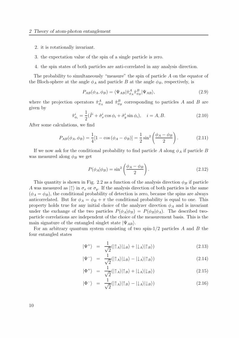
For an arbitrary quantum system consisting of two spin-1/2 particles A and B thefour entangled states
|Ψ+〉 =1√2(|↑A〉|↓B〉 + |↓A〉|↑B〉) (2.13)
|Ψ−〉 =1√2(|↑A〉|↓B〉 − |↓A〉|↑B〉) (2.14)
|Φ+〉 =1√2(|↑A〉|↑B〉 + |↓A〉|↓B〉) (2.15)
|Φ−〉 =1√2(|↑A〉|↑B〉 − |↓A〉|↓B〉) (2.16)
10

2.3 Entanglement
0 2 4 6 8
0.2
0.4
0.6
0.8
1
φb (rad)
P(
|
)
φφ
ab
Figure 2.2: Expected spin correlations of an entangled state |ΨAB〉 for complementarymeasurement bases of particle A as the analyzer-direction of particle B isvaried by an angle φB . (Red line) particle A is measured along φA = 0corresponding to |↑〉x. (Blue line) particle A is analyzed along φA = π/2corresponding to |↑〉y.
form an orthonormal basis of the 2 × 2 dimensional Hilbert space. These states arecalled Bell states and violate a Bell inequality (see subsection 2.3.2) by the maximumvalue predicted by quantum mechanics. Furthermore the Bell states have the importantproperty that each state can be transformed into any other of the four Bell states byunitary single particle rotations.
2.3.1 The EPR “paradox”
Every spin-entangled state has the property that none of the two spins has a definedvalue. Therefore it is impossible to predict the outcome of a spin measurement on oneparticle with certainty. But if we perform a measurement on one spin, instantaneouslythe outcome of a spin measurement on the other particle is known. This holds trueeven if the spins are separated by an arbitrary distance. These counterintuitive featuresof entangled quantum systems were used by Einstein, Podolsky and Rosen (EPR) [2]to argue that the quantum mechanical description of the physical reality can not beconsidered complete. EPR understand a theory to be complete if every element of thephysical reality is represented in the physical theory in the sense that:
“If, without in any way disturbing a system, we can predict with certainty (i.e. withprobability equal to unity) the value of a physical quantity, then there exists an elementof physical reality corresponding to this quantity.”
The first part of the reality criterion requires that the prediction can be made withoutdisturbing the object in question. It is, for instance, possible to predict the value of the
11

2 Theory of atom-photon entanglement
mass of the next pion crossing a bubble chamber without interacting with it. In everycase in which the prediction can be made in this way, the EPR reality criterion assignsto the object an element of reality, i.e., something real that does not necessarily coincidewith the observed property but generates it deterministically when a measurement ismade.
Furthermore EPR require that any physical theory has to be local. In other wordsthe locality postulate is based on the reasonable belief that the strength of interactionbetween objects depends inversily on their separation. If an electron is observed in alaboratory, another electron 10 or 1010 m away acquires no new property. To summarize,the idea of locality can be formulated as follows:
“Given two separated objects A and B, the modifications of A due to anything thatmay happen to B can be made arbitrarily small for any measurable physical quantity, byincreasing their separation.”
In 1951 David Bohm restated and simplified the EPR argument on the basis of thespin-entangled state |ΨAB〉 from (2.8) as follows [37]:
1. Pick an arbitrary analysis basis, e.g. the z-basis and measure the spin of particleA. Then the result will be either ↑ or ↓, say ↑.
2. Knowing that the spin of particle A is “up”, we know with certainty that the resultof a spin-measurement of B will be “down”. But if we then measure particle B inthe x-basis we will find that particle B has a definite spin (either ↑x or ↓x), i.e.,we know the value of σx.
3. Therefore, we know both the z and x components of the spin of particle B, whichis a violation of complementarity.
In the words of EPR this implies a very unsatisfactory state of affairs: “Thus, it ispossible to assign two different state vectors to the same reality.” One way out of thisproblem is to argue that in a single experiment one can measure particle B only in onebasis and not in two bases at the same time. The knowledge of a fictitious measurementresult does not replace the measurement process itself. From this point of view theEPR assumption about elements of reality becomes useless: it can only lead to theconclusion that “an element of reality is associated with a concretely performed act ofmeasurement”. This argument was used by Bohr [38] in a reply to EPR, whereas EPRused the inability of quantum mechanics to make definite predictions for the outcomeof a certain measurement to postulate the existence of “hidden” variables which are notknown and perhaps not measurable. It was hoped that an inclusion of these hiddenvariables (LHV) would restore the completness and determinism to the quantum theory.
12
2.3 Entanglement
2.3.2 Bell’s inequality
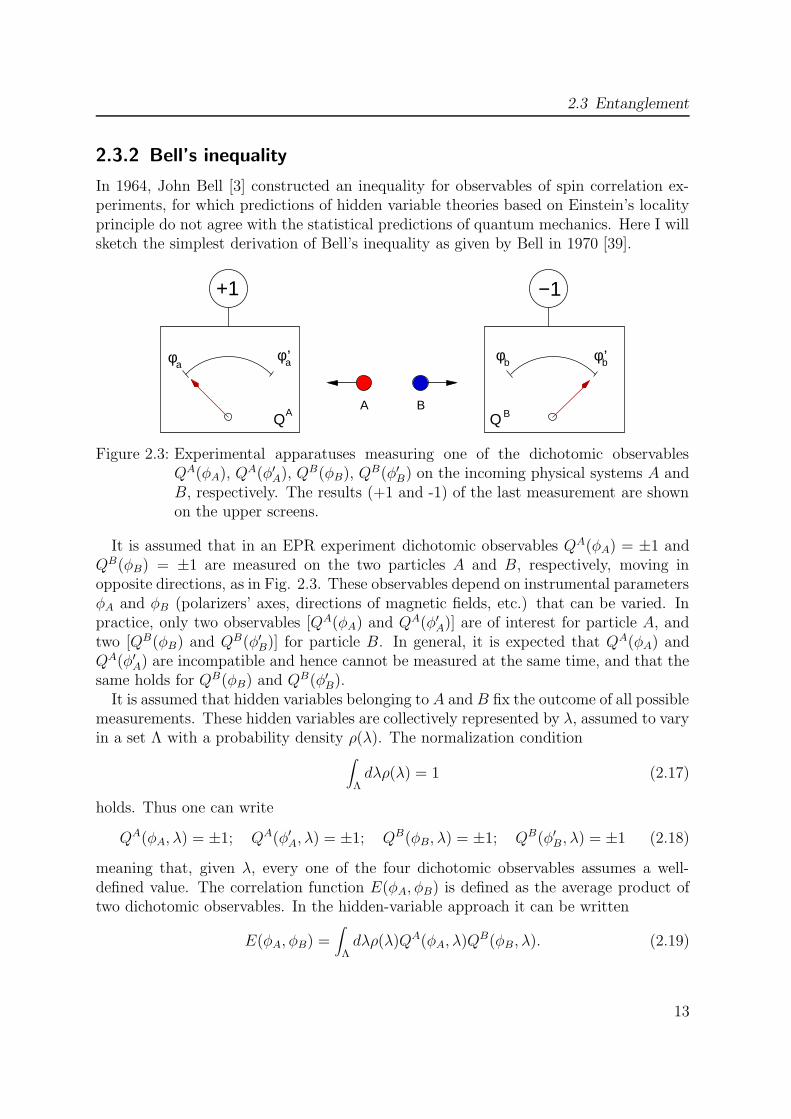
In 1964, John Bell [3] constructed an inequality for observables of spin correlation ex-periments, for which predictions of hidden variable theories based on Einstein’s localityprinciple do not agree with the statistical predictions of quantum mechanics. Here I willsketch the simplest derivation of Bell’s inequality as given by Bell in 1970 [39].
φaφa’ φb ’φb
A B
+1 −1
QA Q B
Figure 2.3: Experimental apparatuses measuring one of the dichotomic observablesQA(φA), QA(φ′
A), QB(φB), QB(φ′B) on the incoming physical systems A and
B, respectively. The results (+1 and -1) of the last measurement are shownon the upper screens.
It is assumed that in an EPR experiment dichotomic observables QA(φA) = ±1 andQB(φB) = ±1 are measured on the two particles A and B, respectively, moving inopposite directions, as in Fig. 2.3. These observables depend on instrumental parametersφA and φB (polarizers’ axes, directions of magnetic fields, etc.) that can be varied. Inpractice, only two observables [QA(φA) and QA(φ′
A)] are of interest for particle A, andtwo [QB(φB) and QB(φ′
B)] for particle B. In general, it is expected that QA(φA) andQA(φ′
A) are incompatible and hence cannot be measured at the same time, and that thesame holds for QB(φB) and QB(φ′
B).It is assumed that hidden variables belonging to A and B fix the outcome of all possible
measurements. These hidden variables are collectively represented by λ, assumed to varyin a set Λ with a probability density ρ(λ). The normalization condition
∫
Λdλρ(λ) = 1 (2.17)
holds. Thus one can write
QA(φA, λ) = ±1; QA(φ′A, λ) = ±1; QB(φB, λ) = ±1; QB(φ′
B, λ) = ±1 (2.18)
meaning that, given λ, every one of the four dichotomic observables assumes a well-defined value. The correlation function E(φA, φB) is defined as the average product oftwo dichotomic observables. In the hidden-variable approach it can be written
E(φA, φB) =∫
Λdλρ(λ)QA(φA, λ)QB(φB, λ). (2.19)
13

2 Theory of atom-photon entanglement
This is a local expression, in the sense that neither QA depends on φB nor QB on φA.It is easy to show that [39]
|E(φA, φB) − E(φA, φ′B) + E(φ′
A, φB) + E(φ′A, φ
′B)|
≤∫
Λdλ|QA(φA, λ)||QB(φB, λ) −QB(φ′
B, λ)| + |QA(φ′A, λ)||QB(φB, λ) −QB(φ′
B, λ)|
=∫
Λdλ|QB(φB, λ) −QB(φ′
B, λ)| + |QB(φB, λ) −QB(φ′B, λ)|
since |QA(φA, λ)| = |QA(φ′A, λ)| = 1. But the moduli QB(φB, λ) and QB(φ′
B, λ) are alsoequal to 1, so
|QB(φB, λ) −QB(φ′B, λ)| + |QB(φB, λ) +QB(φ′
B, λ)| = 2 (2.20)
From (2.17) and (2.20) one obtains the inequality
S(φA, φB, φ′A, φ
′B) = |E(φA, φB) − E(φA, φ
′B)| + |E(φ′
A, φB) + E(φ′A, φ
′B)| ≤ 2. (2.21)
This is Bell’s inequality in the CHSH form [40], which is more general than its originalform [3].
The present proof is based on a general form of realism because the hidden variable λis thought to belong objectively to the real physical systems A and B. It is also basedon locality for three reasons: (1) the dichotomic observables QA and QB do not dependon the parameters φA and φB of the experimental apparatus; (2) the probability densityρ(λ) does not depend on φA and φB; (3) the set Λ of possible λ values does not dependon φA and φB. The time arrow assumption is also implicit in the dependance of ρ(λ) onφ. In principle, the choices of the values of the instrumental parameters could be madewhen the particles A and B are in flight from the source to the analyzers.
But now, supposed two particles are in the entangled singlet state |ΨAB〉. Quantummechanically, the measurement of the dichotomic variables QA and QB is represented bythe spin operators ~σA~a and ~σB~b. The corresponding quantum mechanical correlationsentering Bell’s inequality are given by the expectation value for the product of spin-measurements on particle A and B along the directions ~a and ~b:
EQM(~a,~b) = 〈ΨAB|~σA~a⊗ ~σB~b|ΨAB〉
=1
2(〈↑|~σA~a|↑〉〈↓|~σB~b|↓〉 − 〈↑|~σA~a|↓〉〈↓|~σB~b|↑〉
−〈↓|~σA~a|↑〉〈↑|~σB~b|↓〉 + 〈↓|~σA~a|↓〉〈↑|~σB~b|↑〉)= −~a~b = cos (φA − φB)
Choosing the directions φA = 0, φ′A = π/2, φB = π/4 and φ′
B = 3π/4 of the spinanalyzers, one finds a maximal violation of inequality (2.21), namely
SQM(0, π/2, π/4, 3π/4) = 2√
2 > 2. (2.22)
14

2.3 Entanglement
Thus, for the spin entangled singlet state, the quantum mechanical correlations betweenthe measurement results of two distant observers are stronger than any possible corre-lation predicted by LHV theories.
The great achievement of John Bell was, that he derived a formal expression whichallows to distinguish experimentally between local-realistic theories and quantum theory.In real experiments it is hard to violate Bell’s inequality without the additional assump-tion of fair sampling. Pearle [11], for example, noted that a subensemble of detectedevents can agree with quantum mechanics even though the entire ensemble satisfies thepredictions of Bell’s inequality for local-realistic theories.
Clauser-Horne inequality
In 1974 Clauser and Horne derived an inequality, which can be tested in real experimentswith an essential weaker assumption [41]. Supposed during a period of time, while theadjustable parameters of the apparatus have the values φA and φB, the source emits, say,N two-particle systems of interest. For this period, denote by NA(φA) and NB(φB) thenumber of counts at detectors A and B, respectively, and by NAB(φA, φB) the numberof simultaneous counts from the two detectors (coincident events). If N is sufficientlylarge, then the ensemble probabilities of these results are
PA(φA) = NA(φA)/N,
PB(φB) = NB(φB)/N, (2.23)
PAB(φA, φB) = NAB(φA)/N.
After some algebra they obtain
S(φA, φB, φ′A, φ
′B) =
PAB(φA, φB) − PAB(φA, φ′B) + PAB(φ′
A, φB) + PAB(φ′A, φ
′B)
PA(φ′A) + PB(φB)
≤ 1.
(2.24)In this inequality the probabilities can be replaced simply by count rates because thenormalization to the real number of emitted pairs N cancels.
Loopholes
To exclude any local realistic theory in a Bell-type experiment one generally assumes:(1) the detection probability of a pair of particles which has passed the analyzers is in-dependent of the analyzer settings [40]; (2) the detected subset is a sample of the wholeemitted pairs; (3) a distant apparatus does not influence a space-like and time-limitedmeasurement due to any relativistic effect. If any of these assumptions is dropped ahard proof that local-realistic theories can not describe our physical reality is impossi-ble. Most prominently the detection loophole (2) and the locality loophole (3) are usedby critics to argue that no experiment disproves the concept of local realism.
15

2 Theory of atom-photon entanglement
In 1972 Freedman and Clauser [4] published an experiment which was designed fora first test of Bell’s inequality. A cascade transition in 40Ca was used to generatepolarization entangled photon pairs. Ten years later Aspect et al. [5, 6] modified theCa experiments by Clauser in a way that they used a non-resonant two-photon processfor the excitation instead of a Deuterium arc lamp. Furthermore this experiment tookgreat care to use non-absorptive state analyzers and to switch fast between differentmeasurement bases in order to fulfill the requirements assumed by John Bell in hisoriginal work. Aspect et al. retrieved experimental data violating the CHSH-inequalityby 2.697 ± 0.015. A new era of Bell experiments was opened by the application ofthe nonlinear optical effect of parametric down-conversion to generate entangled photonpairs [18]. A sequence of different experiments have been performed which culminatedin two Bell experiments [7, 42] highlighting the strict relativistic separation betweenmeasurements. But both experiments suffered from low detection efficiencies allowingthe possibility that the subensemble of detected events agrees with quantum mechanicseven though the entire ensemble satisfies the predictions of Bell’s inequalities for local-realistic theories. This loophole is referred to as detection loophole and was addressedin an experiment with two trapped ions [8], whereby the quantum state detection ofthe atoms was performed with almost perfect efficiency. But the ion separation was notlarge enough to eliminate the locality loophole.
2.3.3 Quantifying entanglement
The quantification of entanglement is a long standing problem in quantum informationtheory. Any good measure of entanglement should satisfy certain conditions. An im-portant condition is that entanglement cannot increase by local operations and classicalcommunications (for more detail see [43]). The question which amount of entanglementis contained in an arbitrary two-particle quantum state represented by a density matrixρ is connected closely to the general question “how close are two quantum states”. Onemeasure of distance between quantum states is the fidelity F .
For an unknown quantum system consisting of two spin-1/2 particles the state isrepresented by a 4 × 4 density matrix ρ. The entanglement fidelity with respect to aparticular maximally entangled pure state |ΨAB〉 is given by [44]
F (|ΨAB〉, ρ) = 〈ΨAB|ρ|ΨAB〉 =1
2(〈↓↑|ρ|↓↑〉+ 〈↑↓|ρ|↑↓〉+ 〈↓↑|ρ|↑↓〉+ 〈↑↓|ρ|↓↑〉), (2.25)
the overlap between |Ψ〉 and ρ. The first two terms in this expression are the measuredconditional probabilities of detecting |↓〉A|↑〉B and |↑〉A|↓〉B. The last two terms can bedetermined by repeating the experiment while rotating each spin through a polar angleof π/2 in the Bloch sphere before measurement. The rotated quantum state is thengiven by ρ. Without a complete state tomography of ρ the entanglement fidelity F can
16

2.3 Entanglement
not be determined accurately. But one can derive a lower bound of F , expressed onlyin terms of diagonal density matrix elements in the original and rotated basis [35]:
F ≥ 1
2(〈↓↑|ρ|↓↑〉 + 〈↑↓|ρ|↑↓〉 − 2
√
〈↓↓|ρ|↓↓〉〈↑↑|ρ|↑↑〉 + 〈↓↑|ρ|↓↑〉 + 〈↑↓|ρ|↑↓〉−〈↓↓|ρ|↓↓〉 − 〈↑↑|ρ|↑↑〉) (2.26)
Another possibility to determine the entanglement fidelity of an unknown quantumstate ρ is to do the following. Suppose, a source emits two spin-1/2 particles in theentangled pure state |ΨAB〉. But due to experimental imperfections in the state detectionof spin A and B, the state |ΨAB〉 can be measured with the probability 0 ≤ p ≤ 1. Forthe rest of the unperfect state we expect white noise, corresponding to the maximallymixed state 1
4I. Technically speaking, the imperfect detection is modeled by an ideal
preparation accompanied/followed by a noisy channel, which transforms the maximallyentangled initial state ρ = |ΨAB〉〈ΨAB| as
ρ→ ρ = p|ΨAB〉〈ΨAB| +(1 − p)
4I , (2.27)
where I is the identity operator. If we plug this expression into the definition of theentanglement fidelity F in Eq. 2.25, we obtain
F = p+(1 − p)
4(2.28)
For a mixed state denoted by a density matrix ρ, the correlations entering a Bell in-equality are given by
E(~a,~b) = Trρ~σA~a⊗ ~σB~b =4∑
i,k
〈ui|ρ|uk〉〈uk|~σA~a⊗ ~σB~b|ui〉, (2.29)
where |ui〉 denotes the two particle spin-1/2 basis states |↑↑〉, |↑↓〉, |↓↑〉 and |↓↓〉. Onthe basis of the mixed state density matrix (2.27) and (2.29) it is possible to derive theminimal amount of entanglement necessary to violate a Bell inequality. One obtainsp ≥ 0.707 corresponding to a minimum entanglement fidelity of F = 0.78. For fidelitiesF > 0.5, the underlying quantum state is entangled [44].
2.3.4 Applications of entanglement
Until the early 1990s the general physical interest concerning entanglement was focusedon fundamental tests of quantum mechanics. But in 1991 A. Ekert [45] realized thatthe specific correlations of entangled spin-1/2 particles and Bell’s theorem can be usedto distribute secret keys. Two years later Bennet, Brassard, Crepeau, Josza, Peres andWootters [46] proposed to transfer the quantum state of a particle to another particle at
17

2 Theory of atom-photon entanglement
ΨAΨBC
ΨC
entangled stateinitial state
B CA
Bell analyzer U
classical information
Alice Bob
teleported state
Figure 2.4: Principle of quantum teleportation using two-particle entanglement. Aliceperforms a Bell state measurement on the initial particle and particle B.After she has sent the measurement result as classical information to Bob,he performes a unitary transformation (U) on particle C depending on Alice’measurement result to reconstruct the initial state.
a distant location employing entanglement as a resource, and it was realized by Zukowskiet al. [15] that two particles can be entangled by a projection measurement on entangledBell-states although they never interacted in the past. In the last decade the physicalinterest about entanglement focused also on applications for computational tasks. Onthe next pages I will give a short review on quantum teleportation and entanglementswapping because entanglement between a single atom and a single photon can be usedto map quantum information between light- and matter-based quantum systems and forentangling space-like separated atoms for a loophole-free test of Bell’s inequality.
Quantum Teleportation
The idea of of quantum teleportation [46] is that Alice has a spin-1/2 particle in a certainquantum state |ΨA〉 = a|↑A〉+ b|↓A〉. She wishes to transfer this quantum state to Bob,but she cannot deliver the particle directly to him because their only connection is viaa classical channel. According to the projection postulate of quantum mechanics weknow that any quantum measurement performed by Alice on her particle will destroythe quantum state at hand without revealing all the necessary information for Bob toreconstruct the quantum state. So how can she provide Bob with the quantum state?The answer is to use an ancillary pair of entangled particles B and C in the singlet state
|Ψ−BC〉 =
1√2(|↑B〉|↓C〉 − |↓B〉|↑C〉) (2.30)
shared by Alice and Bob.
18
2.3 Entanglement
Although initially particles A and B are not entangled, their joint state can alwaysbe expressed as a superposition of four maximally entangled Bell states, given by (2.13),since these states form a complete orthonormal basis. The total state of the threeparticles can be written as:
|ΨABC〉 = |ΨA〉 ⊗ |ΨBC〉 =1
2[ |Ψ−
AB〉 ⊗ (−a|↑C〉 − b|↓C〉)+ |Ψ+
AB〉 ⊗ (−a|↑C〉 + b|↓C〉)+ |Φ−
AB〉 ⊗ (+a|↓C〉 + b|↑C〉)+ |Φ+
AB〉 ⊗ (+a|↓C〉 − b|↑C〉)]. (2.31)
Alice now performs a Bell state measurement (BSM) on particles A and B, that is, sheprojects her two particles onto one of the four Bell states. As a result of the measurementBob’s particle will be found in a state that is directly related to the initial state. Forexample, if the result of Alice’s Bell state measurement is |Φ−
AB〉 then particle C in thehands of Bob is in the state a|↓C〉+ b|↑C〉. All that Alice has to do is to inform Bob viaa classical communication channel on her measurement result and Bob can perform theappropriate unitary transformation (U) on particle C in order to obtain the initial stateof particle A.
Entanglement Swapping
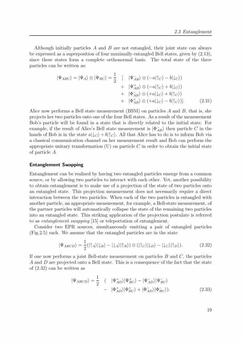
Entanglement can be realized by having two entangled particles emerge from a commonsource, or by allowing two particles to interact with each other. Yet, another possibilityto obtain entanglement is to make use of a projection of the state of two particles ontoan entangled state. This projection measurement does not necessarily require a directinteraction between the two particles. When each of the two particles is entangled withanother particle, an appropriate measurement, for example, a Bell-state measurement, ofthe partner particles will automatically collapse the state of the remaining two particlesinto an entangled state. This striking application of the projection postulate is referredto as entanglement swapping [15] or teleportation of entanglement.
Consider two EPR sources, simultaneously emitting a pair of entangled particles(Fig.2.5) each. We assume that the entangled particles are in the state
|ΨABCD〉 =1
2(|↑A〉|↓B〉 − |↓A〉|↑B〉) ⊗ (|↑C〉|↓D〉 − |↓C〉|↑D〉). (2.32)
If one now performs a joint Bell-state measurement on particles B and C, the particlesA and D are projected onto a Bell state. This is a consequence of the fact that the stateof (2.32) can be written as
|ΨABCD〉 =1
2( |Ψ+
AD〉|Ψ+BC〉 − |Ψ−
AD〉|Ψ−BC〉
− |Φ+AD〉|Φ+
BC〉 + |Φ−AD〉|Φ−
BC〉). (2.33)
19

2 Theory of atom-photon entanglement
Bell StateMeasurement
BA C D
EPR−source I EPR−source II
Figure 2.5: Principle of entanglement swapping. Two sources produce two pairs of en-tangled particles, pair A-B and pair C-D. One particle from each pair (par-ticles B and C) is subjected to a Bell-state measurement. This results in aprojection of particles A and D onto an entangled state.
In all cases particles A and D emerge entangled, despite the fact that they never inter-acted in the past.
2.4 Atom-photon entanglement
When a single atom is prepared in an excited state |e〉 it can spontaneously decay to theground level |g〉 and emit a single photon. Due to conservation of angular momentumin spontaneous emission the polarization of the emitted photon is correlated with thefinal quantum state |g〉 of the atom. For a simple two-level atom, after spontaneousemission, the system is in a tensor product state of the atom and the photon. But formultiple decay channels to different ground states the resuling state of atom and photonis entangled.
The physical process of spontaneous emission can not be explained by a semiclassicaltreatment of the light field but only by a quantum field approach (this can be foundin [47]). I do not intend to give a sophisticated treatment of spontaneous emission,but I rather give a phenomenological approach, which will be sufficient to understandatom-photon entanglement in the context of the present work.
2.4.1 Weisskopf-Wigner theory of spontaneous emission
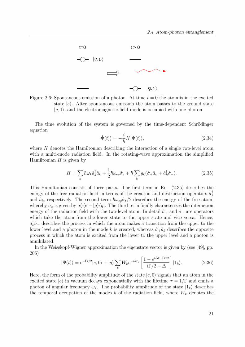
Let us consider a single atom at time t = 0 in the excited state |e〉 and the field modesin the vacuum state |0〉. In the “dressed state picture” the state of the system is thengiven by |e, 0〉 = |e〉 ⊗ |0〉, the product of the atomic state |e〉 and the vacuum state |0〉of the electromagnetic field. Due to coupling of the atom to vacuum fluctuations of theelectromagnetic field (this can be found in [48]) the atom will decay with a characteristictime constant τ , called the natural lifetime, to the ground state |g〉 and emit a singlephoton into the field mode k. For t → ∞ the sytem atom+photon will be in the state|g, 1〉.
20
2.4 Atom-photon entanglement
g,1
e,0
t=0 t > 0
Figure 2.6: Spontaneous emission of a photon. At time t = 0 the atom is in the excitedstate |e〉. After spontaneous emission the atom passes to the ground state|g, 1〉, and the electromagnetic field mode is occupied with one photon.
The time evolution of the system is governed by the time-dependent Schrodingerequation
|Ψ(t)〉 = − i
hH|Ψ(t)〉, (2.34)
where H denotes the Hamiltonian describing the interaction of a single two-level atomwith a multi-mode radiation field. In the rotating-wave approximation the simplifiedHamiltonian H is given by
H =∑
k
hωka†kak +
1
2hωegσz + h
∑
k
gk(σ+ak + a†kσ−). (2.35)
This Hamiltonian consists of three parts. The first term in Eq. (2.35) describes theenergy of the free radiation field in terms of the creation and destruction operators a†kand ak, respectively. The second term hωegσz/2 desrcibes the energy of the free atom,whereby σz is given by |e〉〈e|−|g〉〈g|. The third term finally characterizes the interactionenergy of the radiation field with the two-level atom. In detail σ+ and σ− are operatorswhich take the atom from the lower state to the upper state and vice versa. Hence,a†kσ− describes the process in which the atom makes a transition from the upper to thelower level and a photon in the mode k is created, whereas σ+ak describes the oppositeprocess in which the atom is excited from the lower to the upper level and a photon isannihilated.
In the Weisskopf-Wigner approximation the eigenstate vector is given by (see [49], pp.206)
|Ψ(t)〉 = e−Γt/2|e, 0〉 + |g〉∑
k
Wke−ikr0
[
1 − ei∆t−Γt/2
iΓ/2 + ∆
]
|1k〉. (2.36)
Here, the form of the probability amplitude of the state |e, 0〉 signals that an atom in theexcited state |e〉 in vacuum decays exponentially with the lifetime τ = 1/Γ and emits aphoton of angular frequency ωk. The probability amplitude of the state |1k〉 describesthe temporal occupation of the modes k of the radiation field, where Wk denotes the
21

2 Theory of atom-photon entanglement
∆ m = +/−1∆ m = 0
z zθθ
Figure 2.7: Emission characteristics of light emitted from dipole transitions with ∆m =0,±1.
overlap between the atomic states |g〉 and |e〉 in the field mode k, and ∆ = ωk−ωeg thedetuning in respect to the atomic transition frequency ωeg. For times long compared tothe radiative decay the first term in (2.36) is negligible and the state of the system isgiven by a linear superposition of single-photon states with different wave vectors.
2.4.2 Properties of the emitted photon
Because atomic states are eigenstates of the total angular momentum, the modes of theelectromagnetic field after spontaneous emission are also eigenstates of angular momen-tum. Therefore the polarization state of a photon spontaneously emitted from an atomicdipole depends upon the change in angular momentum ∆m of the atom along the dipoleaxis, and the direction of the emission. For ∆m = 0,±1, the polarization state of aspontaneously emitted photon is
|Π0〉 = sin θ |π〉 for ∆m = 0 (2.37)
|Π±1〉 =√
1 + cos2 θ/√
2 |σ±〉 for ∆m = ±1, (2.38)
where θ is the spherical polar angle with respect to the dipole (quantization) axis, and|π〉 and |σ±〉 denote the polarization state of the photon. Note that along a viewing axisparallel to the dipole (θ = 0) only |σ±〉-polarized radiation is emitted.
2.4.3 Spontaneous emission as a source of atom-photon
entanglement
Until now we considered a single atom in free space which spontaneously emits a photonfrom a two-level transition. According to Weisskopf and Wigner the state of the systematom+photon is a simple tensor product state of the form |g〉|Π∆m〉, where the atom isin the ground state |g〉 and the photon in the state |Π∆m〉. For multiple decay channels
22

2.4 Atom-photon entanglement
0,0
S 1/2
2
P 3/2
2
σ+ σ−
1,−1 1,+11,0
780 nm
F=1
F=2
F=0
Figure 2.8: Atomic level structure in 87Rb used to generate atom-photon entanglement.Provided the emission frequencies for σ+, σ− and π polarized transitions areindistinguishable within the natural linewidth of the transition, the polar-ization of a spontaneously emitted photon will be entangled with the spinstate of the atom.
of spontaneous emission to different ground states of atomic angular momentum F , theresulting (unnormalized) state of photon and atom is
|Ψ〉 =∑
∆m
C∆m|F∆m〉|Π∆m〉, (2.39)
where C∆m are atomic Clebsch-Gordon coefficients for the possible decay channels and|F∆m〉 denote the respective atomic ground states. The state in (2.39) can not berepresented as a tensor product, only as a linear superposition of different productstates. Therefore the spin degree of freedom of the atom and the polarization of thephoton are entangled.
In the current experiment we excite a single 87Rb atom to the 2P3/2, |F = 0, mF = 0〉state by a short optical π-pulse. In the following spontaneous emission the atom decayseither to the |1,−1〉 ground state while emitting a |σ+〉-polarized photon, or to the |1, 0〉state while emitting a |π〉-polarized photon, or to the |1,+1〉 ground state and emits a|σ−〉-polarized photon. Provided these decay channels are spectrally indistinguishable,a coherent superposition of the three possibilities is formed and the magnetic quantumnumber mF of the atom is entangled with the polarization of the emitted photon resultingin the atom-photon state
|Ψ〉 =1√2
[
√
(1 + cos2 θ)/2(
|1,−1〉|σ+〉 + |1,−1〉|σ−〉)
+ sin θ|1, 0〉|π〉]
, (2.40)
where the first index in the atomic basis state |F,mF 〉 denotes the total angular mo-mentum F and the second index indicates the respective magnetic quantum numbermF .
23
2 Theory of atom-photon entanglement
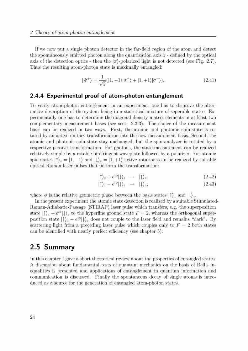
If we now put a single photon detector in the far-field region of the atom and detectthe spontaneously emitted photon along the quantization axis z - defined by the opticalaxis of the detection optics - then the |π〉-polarized light is not detected (see Fig. 2.7).Thus the resulting atom-photon state is maximally entangled:
|Ψ+〉 =1√2(|1,−1〉|σ+〉 + |1,+1〉|σ−〉). (2.41)
2.4.4 Experimental proof of atom-photon entanglement
To verify atom-photon entanglement in an experiment, one has to disprove the alter-native description of the system being in a statistical mixture of seperable states. Ex-perimentally one has to determine the diagonal density matrix elements in at least twocomplementary measurement bases (see sect. 2.3.3). The choice of the measurementbasis can be realized in two ways. First, the atomic and photonic spin-state is ro-tated by an active unitary transformation into the new measurement basis. Second, theatomic and photonic spin-state stay unchanged, but the spin-analyzer is rotated by arespective passive transformation. For photons, the state-measurement can be realizedrelatively simple by a rotable birefringent waveplate followed by a polarizer. For atomicspin-states |↑〉z = |1,−1〉 and |↓〉z = |1,+1〉 active rotations can be realized by suitableoptical Raman laser pulses that perform the transformation:
|↑〉z + eiφ|↓〉z → |↑〉z (2.42)
|↑〉z − eiφ|↓〉z → |↓〉z, (2.43)
where φ is the relative geometric phase between the basis states |↑〉z and |↓〉z.In the present experiment the atomic state detection is realized by a suitable Stimulated-
Raman-Adiabatic-Passage (STIRAP) laser pulse which transfers, e.g. the superpositionstate |↑〉z + eiφ|↓〉z to the hyperfine ground state F = 2, whereas the orthogonal super-position state |↑〉z − eiφ|↓〉z does not couple to the laser field and remains “dark”. Byscattering light from a preceding laser pulse which couples only to F = 2 both statescan be identified with nearly perfect efficiency (see chapter 5).
2.5 Summary
In this chapter I gave a short theoretical review about the properties of entangled states.A discussion about fundamental tests of quantum mechanics on the basis of Bell’s in-equalities is presented and applications of entanglement in quantum information andcommunication is discussed. Finally the spontaneous decay of single atoms is intro-duced as a source for the generation of entangled atom-photon states.
24
3 Single atom dipole trap
3.1 Introduction
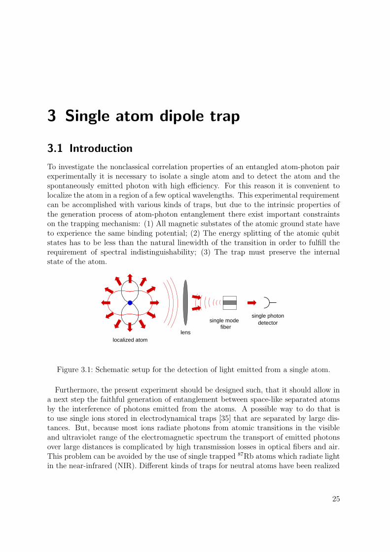
To investigate the nonclassical correlation properties of an entangled atom-photon pairexperimentally it is necessary to isolate a single atom and to detect the atom and thespontaneously emitted photon with high efficiency. For this reason it is convenient tolocalize the atom in a region of a few optical wavelengths. This experimental requirementcan be accomplished with various kinds of traps, but due to the intrinsic properties ofthe generation process of atom-photon entanglement there exist important constraintson the trapping mechanism: (1) All magnetic substates of the atomic ground state haveto experience the same binding potential; (2) The energy splitting of the atomic qubitstates has to be less than the natural linewidth of the transition in order to fulfill therequirement of spectral indistinguishability; (3) The trap must preserve the internalstate of the atom.
lenslocalized atom
single modefiber
single photondetector
Figure 3.1: Schematic setup for the detection of light emitted from a single atom.
Furthermore, the present experiment should be designed such, that it should allow ina next step the faithful generation of entanglement between space-like separated atomsby the interference of photons emitted from the atoms. A possible way to do that isto use single ions stored in electrodynamical traps [35] that are separated by large dis-tances. But, because most ions radiate photons from atomic transitions in the visibleand ultraviolet range of the electromagnetic spectrum the transport of emitted photonsover large distances is complicated by high transmission losses in optical fibers and air.This problem can be avoided by the use of single trapped 87Rb atoms which radiate lightin the near-infrared (NIR). Different kinds of traps for neutral atoms have been realized
25

3 Single atom dipole trap
in the last 20 years, but not all trapping mechanisms are applicable for the investigationof atom-photon and atom-atom entanglement. Magnetic traps [50, 51] are based on thestate-dependent force of the magnetic dipole moment in an inhomogenous field. Hence,this kind of trap is unsuitable for trapping atomic spin states with different sign. Inaddition, magnetic traps do not preserve the spectral indistinguishability of the possi-ble photonic emission paths due to different Zeeman-splitting of the magnetic substatesmF = −1 and mF = +1. The trapping mechanism of Magneto-optical traps (MOT)[52, 53] relies on near resonant scattering of light destroying any atomic coherence on atimescale of the excited state lifetime. Optical dipole traps - first proposed by Letokhovin 1968 [54, 55] - rely on the electric dipole interaction with far-detuned light at whichthe optical excitation can be kept extremely low. In optical dipole traps atomic coher-ence times up to several seconds are possible [56], and under appropriate conditions thetrapping mechanism is independent of the particular magnetic sub-level of the electronicground state. Therefore a localized single 87Rb atom in a far-off-resonance optical dipoletrap satisfies all necessary requirements for the investigation of atom-photon and atom-atom entanglement.
In the context of this thesis our group has set up a microscopic optical dipole trap,which allows to trap single Rubidium atoms one by one with a typical trap life- andcoherence time of several seconds. In order to understand the operating mode of ourtrap I will first indroduce the basic theoretical concepts of atom trapping in opticaldipole potentials. Then I will describe the experimental setup of our dipole trap andmeasurements which prove the subpoissonian occupation statistics. Finally the meankinetic energy of a single atom was determined via the spectral analysis of the emittedfluorescence light.
3.2 Theory of optical dipole traps for neutral atoms
Following Grimm et al. [57] I will introduce the basic concepts of atom trapping inoptical dipole potentials that result from the interaction with far-detuned light. In thiscase of particular interest, the optical excitation is very low and the radiation forcedue to photon scattering is negligible as compared to the dipole force. In Sec. 3.2.1,I consider the atom as a simple classical or quantum-mechanical oscillator to derivethe main equations for the optical dipole interaction. Then the case of real multi-levelatoms is considered, which allows to calculate the dipole potential of the 2S1/2 groundand 2P3/2 excited state in 87Rb. Atom trapping in dipole potentials requires cooling toload the trap and eventually also to counteract heating in the dipole trap. I thereforebriefly review two laser cooling methods and their specific features with respect to ourexperiment. Then I discuss sources of heating, and derive explicit expressions for theheating rate in the case of thermal equilibrium in a dipole trap. Finally I will present asimple model which allows to understand the atom number limitation in a small volume
26

3.2 Theory of optical dipole traps for neutral atoms
dipole trap due to light-induced two-body collisions. This effect opens the possibilityto trap only single atoms and simplifies the experimental investigation of an entangledatom-photon state.
3.2.1 Optical dipole potentials
Oscillator model
The optical dipole force arises from the dispersive interaction of the induced atomicdipole moment with the intensity gradient of the light field [54]. Because of its conser-vative character, the force can be derived from a potential, the minima of which canbe used for atom trapping. The absorptive part of the dipole interaction in far-detunedlight leads to residual photon scattering of the trapping light, which sets limits to theperformance of dipole traps. In the following I will derive the basic equations for thedipole potential and the scattering rate by considering the atom as a simple oscillatorsubject to the classical radiation field.
When an atom is irradiated by laser light, the electric field E induces an atomic dipolemoment p that oscillates at the driving frequency ω. In the usual complex notationE(r, t) = eE(r)eiωt + eE∗(r)e−iωt and p(r, t) = ep(r)eiωt + ep∗(r)e−iωt, where e is theunit polarization vector, the amplitude p of the dipole moment is simply related to thefield amplitude E by
p = α(ω)E. (3.1)
Here α is the complex polarizability, which depends on the driving frequency ω.
The interaction potential of the induced dipole moment p in the driving field E isgiven by
Udip = −1
2〈pE〉 = − 1
2ε0cRe(α)I (3.2)
where <> denote the time average over the rapid oscillating terms. The laser fieldintensity is
I =1
2ε0c|E|2, (3.3)
and the factor 1/2 takes into account that the dipole moment is an induced, not apermanent one. The potential energy of the atom in the field is thus proportional tothe intensity I and to the real part of the polarizability, which describes the in-phasecomponent of the dipole oscillation being responsible for the dispersive properties of theinteraction. The dipole force results from the gradient of the interaction potential
Fdip(r) = −∇Vdip(r) =1
2ε0cRe(α)∇I(r). (3.4)
It is thus a conservative force, proportional to the intensity gradient of the driving field.
27

3 Single atom dipole trap
The power absorbed by the oscillator from the driving field (and re-emitted as dipoleradiation) is given by
Pabs = 〈pE〉 =ω
ε0cIm(α)I(r). (3.5)
The absorption results from the imaginary part of the polarizability, which describes theout-of-phase component of the dipole oscillation. Considering the light as a stream ofphotons hω, the absorption can be interpreted in terms of photon scattering in cyclesof absorption and subsequent spontaneous reemission processes. The correspondingscatteringrate is
ΓSc(r) =Pabshω
=1
hε0cIm(α)I(r). (3.6)
We have now expressed the two main quantities of interest for dipole traps, the in-teraction potential and the scattered radiation power, in terms of the position dependentintensity I(r) and the polarizibility α(ω). These expressions are valid for any polarizableneutral particle in an oscillating electric field. This can be an atom in a near-resonantor far off-resonant laser field, or even a molecule in an optical or microwave field.
In order to calculate its polarizability α, I first consider the atom in Lorenz’s model asa classical oscillator (see, e.g. [58]). In this simple and very useful picture, an electron(mass me, elementary charge e) is considered to be bound elastically to the core with anoscillation eigenfrequency ω0 corresponding to the optical transition frequency. Dampingresults from the dipole radiation of the oscillating electron according to Larmor’s well-known formula for the power radiated by an accelerated charge.
It is straightforward to calculate the polarizability by integration of the equation ofmotion
x+ Γω x + ω20x = −eE(t)
me(3.7)
for the driven oscillation of the electron with the result
α =e2
me
1
ω20 − ω2 − iωΓω
. (3.8)
Here
Γω =e2ω2
6πε0mec2(3.9)
is the classical damping rate due to the radiative energy loss. Introducing the on-resonance damping rate Γ ≡ Γω0 = (ω0
ω)2Γω, one can put Eq. 3.8 into the form
α(ω) = 6πε0c2 Γ/ω2
0
ω20 − ω2 − i(ω3/ω2
0)Γ. (3.10)
In a semiclassical approach the atomic polarizability can be calculated by consideringthe atom as a two-level quantum system interacting with a classical radiation field. Whensaturation effects can be neglected, the semiclassical calculation yields the same result as
28
3.2 Theory of optical dipole traps for neutral atoms
the classical calculation with only one modification, the damping rate Γ (correspondingthe spontaneous decay rate of the excited state) is determined by the dipole matrixelement 〈e|µ|g〉 between the ground state |g〉 and the excited state |e〉 by
Γ =ω3
0
3πε0hc2|〈e|µ|g〉|2. (3.11)
For many atoms with a strong dipole-allowed transition starting from its ground state,the classical formula Eq. 3.9 nevertheless provides a good approximation to the sponta-neous decay rate. For the D lines of the alkali atoms Na, K, Rb, and Cs, the classicalresult agrees with the true decay rate to within a few percent.
An important difference between the quantum-mechanical and the classical oscillatoris the possible occurence of saturation. At very high intensities of the driving field, theexcited state gets strongly populated and the classical result (Eq. 3.10) is no longer valid.For dipole trapping, however one is essentially interested in the far-detuned case withvery low saturation and thus very low scatttering rates (ΓSc Γ). Thus the expressionin Eq. 3.10 for the atomic polarizability can be used as an excellent approximation forthe quantum-mechanical oscillator and the explicit expressions for the dipole potentialUdip and the scattering rate ΓSc can be derived.
Udip(r) = −3πc2
2ω30
(
Γ
ω0 − ω+
Γ
ω0 + ω
)
I(r) (3.12)
ΓSc(r) =3πc2
2hω30
(
ω
ω0
)3 ( Γ
ω0 − ω+
Γ
ω0 + ω
)2
I(r) (3.13)
These general expressions are valid for any driving frequency ω and show two resonantcontributions: Besides the usually considered resonance at ω = ω0, there is also theso-called counter-rotating term resonant at ω = −ω0.
In most experiments, the laser is tuned relatively close to the resonance ω0 such thatthe detuning ∆ = ω − ω0 fulfills |∆| ω0. In this case, the counter-rotating term canbe neglected in the well-known rotating wave approximation and the general expressionsfor the dipole potential and the scattering rate simplify to
Udip(r) =3πc2
2ω30
(
Γ
∆
)
I(r), (3.14)
ΓSc(r) =3πc2
2hω30
(
Γ
∆
)2
I(r). (3.15)
The basic physics of dipole trapping in far-detuned laser fields can be understood on thebasis of these two equations. Obviously, a simple relation exists between the scatteringrate and the dipole potential,
hΓSc =Γ
∆Udip. (3.16)
29

3 Single atom dipole trap
Equation 3.14 and 3.15 show two essential points for dipole trapping. First: below anatomic resonance (“red” detuned, ∆ < 0) the dipole potential is negative and the inter-action thus attracts atoms into the light field. Potential minima are therefore found atpositions with maximum intensity. Above resonance (“blue” detuned, ∆ > 0) the dipoleinteraction repels atoms out of the field, and potential minima correspond to minima ofthe intensity. Second: the dipole potential scales as I/∆, whereas the scattering ratescales as I/∆2. Therefore, optical dipole traps usually use large detunings and highintensities to keep the scattering rate as low as possible for a certain potential depth.
Dressed state picture
In terms of the oscillator model, multi-level atoms can be described by state-dependentatomic polarizabilies. An alternative description of dipole potentials is given by thedressed state picture [47] where the atom is considered together with a quantized lightfield. In its ground state the atom has zero internal energy and the field energy is nhωdepending on the number of photons. When the atom is put into an excited state byabsorbing a photon, the sum of its internal energy hω0 and the field energy (n − 1)hωbecomes Ej = hω0 + (n − 1 )hω = −h∆ij + nhω.
For an atom interacting with laser light, the interaction Hamiltonian is Hint = −µEwith µ = −er representing the electric dipole operator. The effect of far-detuned laserlight on the atomic levels can be treated as a time-independent perturbation in thesecond order of the electric field. Applying this perturbation theory for nondegeneratestates, the interaction Hamiltonian Hint leads to an energy shift of the i-th state withthe unperturbed energy Ei , that is given by
∆Ei =∑
j 6=i
|〈j|Hint |i〉|2Ei − Ej
. (3.17)
For a two-level atom, this equation simplifies to
∆E = ±|〈e|µ|g〉|2∆
|E|2 = ±3πc2
2ω30
Γ
∆I (3.18)
with the plus and the minus sign for the excited and ground state, respectively. Thisoptically induced energy shift (known as Light Shift or AC-Stark shift) of the ground-state exactly corresponds to the dipole potential for the two-level atom in Eq. 3.14.
Semiclassical treatment of multi-level atoms
When calculating the light shift on the basis of the semiclassical treatement for a multi-level atom in a specific electronic ground state |i〉 all dipole allowed transitions to theexcited states |f〉 have to be taken into account. Time-dependent perturbation theory
30

3.2 Theory of optical dipole traps for neutral atoms
h ω
h ω∆ E
∆ E
E
0
0
|e’>
|g’>
|e>
|g>
Figure 3.2: Light shifts for a two-level atom. Red-detuned light (∆ < 0) shifts theground state |g〉 down and the excited state |e〉 up by the energy ∆E.
yields an expression for the energy shift of the atomic levels |i〉 - characterized by theireigenenergies Ei - due to interaction with a time-dependent classical electric field withangular frequency ω, which is given by [59]
∆Ei(ω) =−|E|2
4h
∑
f 6=i|〈i|er|f〉|2
(
1
ωif − ω+
1
ωif + ω
)
, (3.19)
where the sum covers all atomic states |f〉 except for the initial state |i〉, and ωif = ωf−ωidenotes the atomic transition frequencies.
The transition matrix elements 〈i|er|f〉 in general depend on the quantum numbersof the initial state |i〉 respresented by n, J, F,mF and n′, J ′, F,m′
F for the final states|f〉 and upon the laser polarization (ε = 0,±1 for π and σ± transitions respectively).Using the Wigner-Eckart theorem [60], the matrix elements 〈i|er|f〉 can be expressed asa product of a real Clebsch-Gordan coefficient 〈F,mF |F ′, 1, m′
F , ε〉 and a reduced matrixelement 〈F ||er||F ′〉:
〈i|er|f〉 = 〈F ||er||F ′〉〈F,mF |F ′, 1, m′F , ε〉. (3.20)
This reduced matrix element can be further simplified by factoring out the F and F ′
dependence into a Wigner 6j symbol, leaving a fully reduced matrix element 〈J ||er||J ′〉that depends only on the electronic orbital wavefunctions:
〈F ||er||F ′〉 = 〈J ||er||J ′〉(−1)F′+J+I+1
√
(2F ′ + 1)(2J + 1)
(
J J ′ 1F ′ F I
)
6j
. (3.21)
The remaining fully reduced matrix element 〈J ||er||J ′〉 can be calculated from the life-time of the transition J → J ′ via the expression [61]
1
τJJ ′
=ω3if
3πε0hc32J + 1
2J ′ + 1|〈J ||er||J ′〉|2. (3.22)
31

3 Single atom dipole trap
32
32
13
13
Jm = −3/2 −1/2 +1/2 +3/2
P3/2
P1/2
1/2S
Figure 3.3: Reduced level scheme in 87Rb. Dipole matrix elements for π-polarized lightare shown as multiples of 〈J ||er||J ′〉.
On the basis of Eq. 3.19, the Wigner-Eckart theorem and Eq. 3.22 one can derive ageneral expression for the light-shift of any atomic hyperfine state |J, F,mF 〉 couplingto the manifold of final states |J ′, F ′, m′
F 〉f , which is given by
∆E(J, F,mF ) =3πc2I
2
∑
J ′,F ′,m′
F
(2J ′ + 1)(2F ′ + 1)
τJJ ′∆′FF ′ω3
FF ′
(
J J ′ 1F ′ F I
)2
6j
|〈F,mF |F ′, 1, m′F , ε〉|2.
(3.23)For simplicity we have introduced the effective detuning ∆′
FF ′:
1
∆′FF ′
=1
ωFF ′ − ω+
1
ωFF ′ + ω, (3.24)
where ωFF ′ denotes the atomic transition frequency and ω is the frequency of the classicallight field.
Light-shift of the 52S1/2 and 52P3/2 state
In the case of a resolved fine-structure, but unresolved hyperfine structure, one canconsider the atom in spin-orbit coupling, neglecting the coupling of the nuclear spin.The interaction with the laser field can thus be considered in the electronic angularmomentum configuration of the D lines, J = 1/2 → J ′ = 1/2, 3/2.
In this situation, illustrated in Fig. 3.3, one can first calculate the light shifts of thetwo electronic ground states mJ = ±1/2 with the simplified relation
∆E(J,mj , ω) =−|E|2
4h
∑
J ′
|〈J ||er||J ′〉|2∆JJ ′
∑
m′
J
|〈J,mJ |J ′, 1, m′J , ε〉|2. (3.25)
On the basis of this equation, one can derive a general result for the potential of
32

3.2 Theory of optical dipole traps for neutral atoms
0.6 0.8 1 1.2 1.4 1.6 1.8 2
-40
-20
0
20
40
λ (µm)
∆ ν
(MH
z)
S 1/2
3/2P
Figure 3.4: 52S1/2 ground- (dashed blue line) and 52S3/2 excited-state (solid red line)light-shift ∆ν as a function of the dipole laser wavelength λ. At 1.4 µmboth states have the same light shift. In contrast to the ground state, theexcited state Zeeman sub levels m′
F experience different light shifts. Here,we assumed equal occupation of the excited state Zeeman sub-levels andcalculated the mean light shift.
a ground state with total angular momentum J and magnetic quantum number mJ ,which is valid for both linear and circular polarization as long as all optical detuningsstay large compared to the ground- and excited-state hyperfine structure splitting:
Udip(r) =3πc2
2
Γ1/2(1 − εgJmJ)
3ω31/2∆1/2
+Γ3/2(2 + εgJmJ)
3ω33/2∆3/2
I(r). (3.26)
Here gJ = 2 is the well known Lande factor for alkali atoms and ε characterizes the laserpolarization (ε = 0,±1 for linearly and σ± polarized light). The detunings ∆1/2,∆3/2 ofthe laser frequency are referred to the atomic transitions S1/2, J → P1/2 and S1/2, J →P3/2 (the D1 and D2 line).
For linear polarization, both electronic ground states mJ = ±1/2 are shifted by thesame amount because of simple symmetry reasons. After coupling to the nuclear spin,the resulting F,mF states have to remain degenerate like the two original mJ states.Consequently, all magnetic sublevels show the same light shifts.
For circular polarization, the far-off-resonance light field lifts the degeneracy of thetwo magnetic sublevels of the electronic 2S1/2 ground state. In this sense, the circularly
33

3 Single atom dipole trap
2
-20
-2
2
-1
0
1
z/zr
r/w0
Vdip
Figure 3.5: Schematical drawing of a focused Gaussian laser beam and cross section ofthe corresponding trapping profile for a red detuned dipole laser.
polarized light acts like a fictitious magnetic field.
With the help of Eq. 3.23 and the knowledge of the lifetimes of all coupling energylevels, it is possible to calculate the light shift of any Zeeman sub-level in the hyperfinestructure of the states 52S1/2, 52P1/2 and 52P3/2. Due to the coupling of the excited states52P1/2 and 52P3/2 to even higher states (see Fig. A.1), their energy shifts may have thesame sign as the ground state energy shift. Thus, the dipole force can be attractive evenfor an atom in an excited state (see Fig. 3.4), in contrast to the simplified two-levelmodel of Fig. 3.2. There exists a magic wavelength for a linear polarized dipole laserfield, for which the excited state 52P3/2 and the ground state are equally shifted (see Fig.3.4). This wavelength amounts to approximately λ = 1.4 µm, enabling state-insensitiveoptical cooling in the dipole potential.
For the photon scattering rate ΓSc of Rubidium, the same line strength factors arerelevant as for the ground state dipole potential, since absorption and light shifts are de-termined by the same transition matrix elements. For linear polarization one explicitelyobtains
ΓSc(r) =πc2
2h
Γ21/2
ω31/2∆
21/2
+2Γ2
3/2
ω33/2∆
23/2
I(r). (3.27)
34

3.2 Theory of optical dipole traps for neutral atoms
Red-detuned focused-beam trap
A focused Gaussian laser beam tuned far below the atomic resonance frequency repre-sents the simplest way to create a dipole trap. The spatial intensity distribution of afocused Gaussian beam with power P propagating along the z-axis is described by
I(r, z) =2P
πw2(z)exp
(
−2r2
w2(z)
)
(3.28)
where r denotes the radial coordinate. The 1/e2 radius w(z) depends on the axialcoordinate z via
w(z) = w0
√
1 + (z
zR)2 (3.29)
where the focal radius w0 is called beam waist and zR = πw20/λ denotes the Rayleigh
length. From the intensity distribution one can derive the optical potential using Eq.3.19, 3.23, or 3.26. The trap depth U is given by U = |U(r = 0, z = 0)|. The Rayleighlength zR is larger than the beam waist by a factor of πw0/λ. Therefore the potentialin the radial direction is much steeper than in the axial direction.
If the mean kinetic energy kBT of an atomic ensemble is much smaller than thepotential depth U , the extension of the atomic sample is radially small compared tothe beam waist and axially small compared to the Rayleigh range. In this case, theoptical potential can be well approximated by a simple cylindrically symmetric harmonicoscillator
U(r, z) = −U[
1 − 2(
r
w0
)2
−(
z
zR
)2]
. (3.30)
The oscillation frequencies of a trapped atom are given by ωR = (4U/mw20)
1/2 in theradial direction, and ωz = (2U/mz2
R)1/2 in the axial direction. For a trap depth of U = 1mK, a beam waist of w0 = 3.5µm, the oscillation frequencies are ωR/2π = 26.2 kHz andωz/2π = 1.3 kHz.
3.2.2 Trap loading
The standard way to load atoms into a dipole trap is to start from a magneto-opticaltrap (MOT) [62] or an optical molasses, by simply overlapping the dipole trap with theatomic cloud in the MOT, before the latter is turned off. Therefore, efficient coolingtechniques are an essential requirement since the attainable depths of optical dipole trapsare generally below 1 mK. Once atoms are captured, further cooling can be applied tocompensate possible heating mechanisms which would otherwise lead to a loss of atoms.In this section, I briefly discuss methods which are of relevance for trapping a singleatom in a microscopic optical dipole trap.
35
3 Single atom dipole trap
Doppler cooling
Doppler cooling proposed by Hansch & Schawlow in 1975 [63] is based on cycles of near-resonant absorption of a photon and subsequent spontaneous emission resulting in a netatomic momentum change per cycle of one photon momentum hk with k = 2π/λ denot-ing the wavenumber of the absorbed photon. Cooling is counteracted by heating due tothe momentum fluctuations by the recoil of spontaneously emitted photons [64]. Equi-librium between cooling and heating determines the lowest achievable temperature. ForDoppler cooling of two-level atoms in standing waves (“optical molasses”), the minimumtemperature TD is given by
TD =hΓ
2kB, (3.31)
where Γ is the spontaneous decay rate of the cooling transition. For Rubidium 87 theDoppler temperature is 146 µK, which is sufficiently low to load atoms into a dipoletrap. The first demonstration of dipole trapping [65] used Doppler cooling for loadingthe trap and keeping the atoms from beeing heated out.
Polarization gradient cooling
The Doppler temperature is a somewhat artificial limit since it is based on the simplifyingassumption of a two-level atom. Atoms with a more complex level structure like Rbcan be cooled far below TD in standing waves with spatially varying polarizations [66],whereby the cooling mechanisms are based on optical pumping between ground stateZeeman sublevels [67].
With polarization-gradient molasses one can prepare atomic samples at temperatureson the order of ∼ 10Trec with the recoil temperature
Trec =h2k2
m(3.32)
being defined as the temperature associated with the kinetic energy gain by emissionof one photon. Polarization-gradient cooling allows efficient loading of a dipole trap,either by cooling inside a magneto-optical trap (MOT) [62, 68] or by cooling in a shortmolasses phase before transfer into the dipole trap.
Besides enhancing the loading efficiency, polarization-gradient cooling can be applieddirectly to atoms trapped in a dipole potential by subjecting them to near-resonantpolarizations gradients [69]. Since the cooling mechanism relies on the modification ofthe ground-state Zeeman sublevels by the cooling light, a necessary condition for efficientcooling is the independency of the trapping potential from the Zeeman substate [70],which can be easily fulfilled in dipole traps.
36

3.2 Theory of optical dipole traps for neutral atoms
3.2.3 Heating and losses
It is a well-known experimental fact in the field of laser cooling and trapping thatcollisional processes between atoms can lead to substantial trap loss. Here I will discussthe most important features of heating and cold collisions.
Heating rate
A fundamental source of heating is the spontaneous scattering of trap photons, whichdue to its random nature causes fluctuations of the radiation force. In a far-detunedoptical dipole trap, the scattering is completly elastic (or quasi-elastic if a Raman processchanges the atomic ground state).
In general both absorption and spontaneous re-emission processes show fluctuationsand thus both contribute to heating [64]. At large detunings, where scattering processesfollow Poisson statistics, the heating due to fluctuations in absorption corresponds to anincrease of the thermal energy by exactly the recoil energy Erec = kBTrec
2per scattering
event. This first contribution occurs in the propagation direction of the light field and isthus anisotropic. The second contribution is due to the random direction of the photonrecoil in spontaneous emission. This heating also increases the thermal energy by onerecoil energy Erec per scattering event, but distributed over all three dimensions. Inmost cases of interest the trap mixes the motional degrees on a time scale faster than orcomparable to the heating. The overall heating thus corresponds to an increase of thetotal thermal energy by 2Erec in a time Γ−1
sc . Therefore the heating power is given by
Pheat = 2ErecΓsc = kBTrecΓsc. (3.33)
In thermal equilibrium, the mean kinetic energy per atom in a three-dimensional trapis Ekin = 3kBT/2. Introducing the parameter κ ≡ Epot/Ekin as the ratio of potentialand kinetic energy, one can express the mean total energy E as
E =3
2(1 + κ)kBT. (3.34)
The relation between mean energy and temperature (Eq. 3.33) allows to reexpressthe heating power resulting from photon scattering (Eq. 3.34) as a heating rate
T =2/3
1 + κTrecΓsc, (3.35)
describing the corresponding increase of temperature with time.
Collisions
In general, trap loss becomes important if the colliding atoms are not in their absoluteground state. In an inelastic process the internal energy can be released into the atomic
37

3 Single atom dipole trap
2S + S1/22
1/2
2S + P1/22
3/2
2S + P1/22
1/2RE
ener
gy
excitationspont. emission
internuclear distance
FCC
Figure 3.6: Schematic diagram of processes leading to trap loss in an optical dipole trapduring the loading stage in the presence of near resonant cooling light.
motion, causing escape from the trap. Due to the shallowness of optical dipole potentials,even the collisional release of the relatively small amount of energy from transitions inthe hyperfine structure of the atomic ground state 2S1/2 will always lead to trap loss.
Trap loss can also occur as a result of light-assisted binary collisions involving atomsin the excited state (see Fig. 3.6). In the radiative escape process (RE) the atoms gainkinetic energy from their mutual attraction and when a spontaneous photon is emittedthat has less energy than the one that was initially absorbed. The energy differenceappears as kinetic energy and can be enough to eject the atoms out of the trap. In a fine-structure changing collision (FCC) the atoms are excited to the 2S1/2+
2P3/2 molecularpotential. When they reach the short-distance region they may change the molecularstate during the collision leading to the repulsive molecular potential 2S1/2+
2P1/2. Theatoms gain kinetic energy from the transition, which is sufficient for ejection of one orboth atoms out of the trap.
Collisional blockade in microscopic optical dipole traps
During the loading stage of an optical dipole trap, light-assisted binary collisions due tothe presence of MOT light [71] dominate the trap loss. When the dipole trap volume issmall enough, this binary collisions prevent loading of more than one atom [72, 73].
The number N of trapped atoms can be described by the equation
dN
dt= R− γN − β ′N(N − 1), (3.36)
where R is the loading rate, γ the single-particle loss coefficient taking into accountcollisions with the background gas in the vacuum apparatus, and β the two-body loss
38
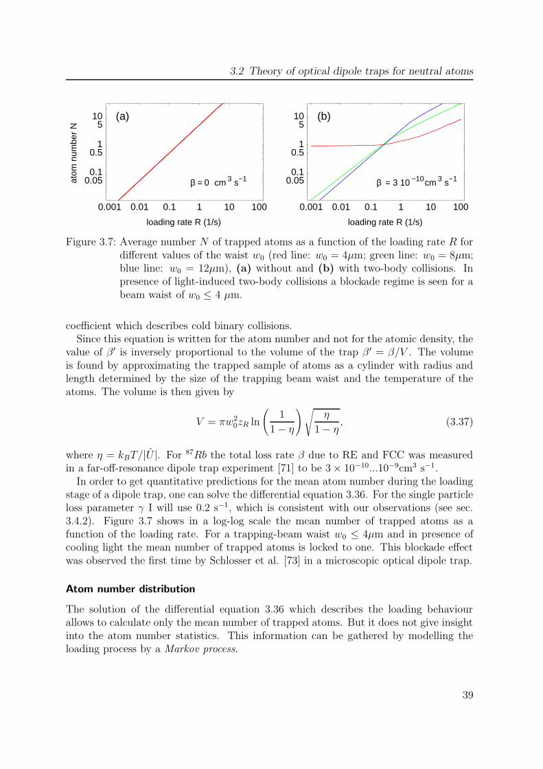
3.2 Theory of optical dipole traps for neutral atoms
0.001 0.01 0.1 1 10 100
0.050.1
0.51
510
0.001 0.01 0.1 1 10 100
0.050.1
0.51
510
cm 3 s−1= 3 10β −10β = 0
loading rate R (1/s) loading rate R (1/s)
(a) (b)
atom
num
ber
N
cm 3 s−1
Figure 3.7: Average number N of trapped atoms as a function of the loading rate R fordifferent values of the waist w0 (red line: w0 = 4µm; green line: w0 = 8µm;blue line: w0 = 12µm), (a) without and (b) with two-body collisions. Inpresence of light-induced two-body collisions a blockade regime is seen for abeam waist of w0 ≤ 4 µm.
coefficient which describes cold binary collisions.Since this equation is written for the atom number and not for the atomic density, the
value of β ′ is inversely proportional to the volume of the trap β ′ = β/V . The volumeis found by approximating the trapped sample of atoms as a cylinder with radius andlength determined by the size of the trapping beam waist and the temperature of theatoms. The volume is then given by
V = πw20zR ln
(
1
1 − η
)√
η
1 − η, (3.37)
where η = kBT/|U |. For 87Rb the total loss rate β due to RE and FCC was measuredin a far-off-resonance dipole trap experiment [71] to be 3 × 10⁻¹⁰...10−9cm3 s−1.
In order to get quantitative predictions for the mean atom number during the loadingstage of a dipole trap, one can solve the differential equation 3.36. For the single particleloss parameter γ I will use 0.2 s−1, which is consistent with our observations (see sec.3.4.2). Figure 3.7 shows in a log-log scale the mean number of trapped atoms as afunction of the loading rate. For a trapping-beam waist w0 ≤ 4µm and in presence ofcooling light the mean number of trapped atoms is locked to one. This blockade effectwas observed the first time by Schlosser et al. [73] in a microscopic optical dipole trap.
Atom number distribution
The solution of the differential equation 3.36 which describes the loading behaviourallows to calculate only the mean number of trapped atoms. But it does not give insightinto the atom number statistics. This information can be gathered by modelling theloading process by a Markov process.
39

3 Single atom dipole trap
Table 3.1: Physical processes and elementary probabilities which lead to a change inthe atom number of +1, -1 and -2.
physical process probability change in Nloading Rdt +1
background collisions γNdt -1two-body collisions β ′N(N − 1)/2 -2
In this modell the overall probability to have N single atoms at a certain time in thedipole trap is represented by a state vector ~r. The change of this state vector per unittime is given by a transfer matrix M which describes the relevant physical processeswhich govern the loading and loss behaviour (see Tab.3.1). In general this matrix is ofdimension (N +1)× (N +1). For simplicity I will restrict myself to the case of maximal5 atoms in the trap and therefore the probability to have 0,1,2,3,4 or 5 atoms in the trapis given by the state vector ~r = (p0, p1, p2, p3, p4, p5) and the transfer matrix by
M =
A1 γ β ′ 0 0 0R A2 2γ 3β ′ 0 00 R A3 3γ 6β ′ 00 0 R A4 4γ 10β ′
0 0 0 R A5 5γ0 0 0 0 R A6
, (3.38)
where AN = 1 − (R +Nγ +N(N − 1)β ′/2) for N = 0, 1, .., 5.The stationary atom number distribution ~rstat is then given by the solution of the
system of linear algebraic equations which can be written as
(M − E)~rstat = ~0, (3.39)
where E is the unity matrix.Now one can calculate the stationary atom number distributions for different loading
rates R relevant for the present experiment (see Fig. 3.8). Here we assume the situationwhen near-resonant colling light is present during the loading stage of the dipole trap.For a dipole laser beam waist of 10 µm we expect poissonian occupation statistics. Inthis regime there is a high probability to trap more than one atom at a time. Whenthe dipole laser beam waist is 3.5µm the probability to load more than one atom isremarkably suppressed leading to subpoissonian occupation statistics. This blockaderegime appears up to a maximum loading rate of 1 atom/s.
40
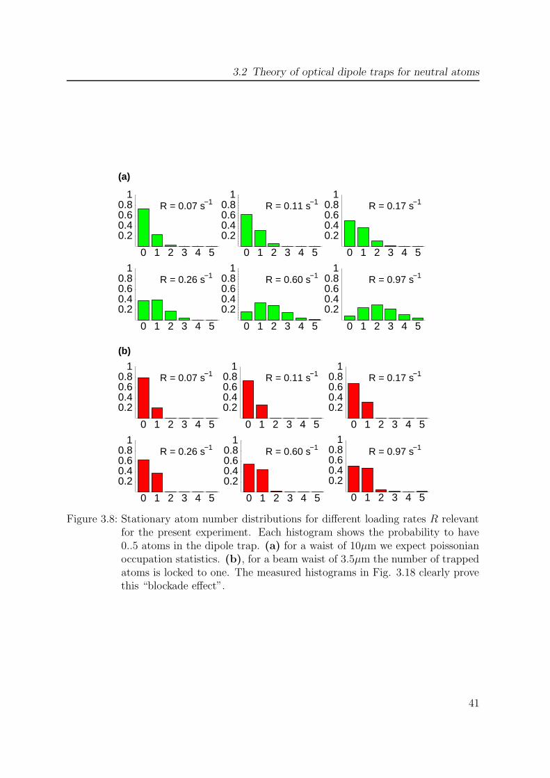
3.2 Theory of optical dipole traps for neutral atoms
0 1 2 3 4 5
0.20.40.60.8
1
0 1 2 3 4 5
0.20.40.60.8
1
0 1 2 3 4 5
0.20.40.60.8
1
0 1 2 3 4 5
0.20.40.60.8
1
0 1 2 3 4 5
0.20.40.60.8
1
0 1 2 3 4 5
0.20.40.60.8
1
0 1 2 3 4 5
0.20.40.60.8
1
0 1 2 3 4 5
0.20.40.60.8
1
0 1 2 3 4 5
0.20.40.60.8
1
0 1 2 3 4 5
0.20.40.60.8
1
0 1 2 3 4 5
0.20.40.60.8
1
0 1 2 3 4 5
0.20.40.60.8
1
R = 0.07 s−1
R = 0.26 s−1
R = 0.11 s−1
R = 0.60 s−1
R = 0.17 s−1
R = 0.97 s−1
R = 0.07 s−1
R = 0.26 s−1 R = 0.60 s−1
R = 0.17 s−1
R = 0.97 s−1
R = 0.11 s−1
(a)
(b)
Figure 3.8: Stationary atom number distributions for different loading rates R relevantfor the present experiment. Each histogram shows the probability to have0..5 atoms in the dipole trap. (a) for a waist of 10µm we expect poissonianoccupation statistics. (b), for a beam waist of 3.5µm the number of trappedatoms is locked to one. The measured histograms in Fig. 3.18 clearly provethis “blockade effect”.
41
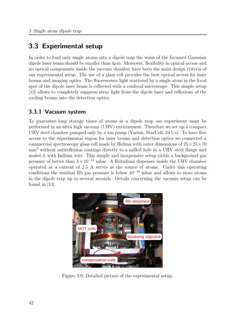
3 Single atom dipole trap
3.3 Experimental setup
In order to load only single atoms into a dipole trap the waist of the focussed Gaussiandipole laser beam should be smaller than 4µm. Moreover, flexibility in optical access andno optical components inside the vaccum chamber have been the main design criteria ofour experimental setup. The use of a glass cell provides the best optical access for laserbeams and imaging optics. The fluorescence light scattered by a single atom in the focalspot of the dipole laser beam is collected with a confocal microscope. This simple setup[13] allows to completely suppress stray light from the dipole laser and reflexions of thecooling beams into the detection optics.
3.3.1 Vacuum system
To guarantee long storage times of atoms in a dipole trap our experiment must beperformed in an ultra high vacuum (UHV) environment. Therefore we set up a compactUHV steel chamber pumped only by a ion pump (Varian, StarCell, 24 l/s). To have freeaccess to the experimental region for laser beams and detection optics we connected acommercial spectroscopy glass cell made by Hellma with outer dimensions of 25×25×70mm3 without antireflexion coatings directly to a milled hole in a UHV steel flange andsealed it with Indium wire. This simple and inexpensive setup yields a background gaspressure of better than 3× 10⁻¹¹ mbar. A Rubidium dispenser inside the UHV chamberoperated at a current of 2.5 A serves as the source of atoms. Under this operatingconditions the residual Rb gas pressure is below 10−10 mbar and allows to store atomsin the dipole trap up to several seconds. Details concerning the vacuum setup can befound in [13].
focussing objective
Rb−dispenser
MOT coils
compensation coils
Figure 3.9: Detailed picture of the experimental setup.
42

3.3 Experimental setup
3.3.2 Laser system
The application of laser cooling and the coherent manipulation of a single atom requirethe lasers to be stabilized onto or near atomic hyperfine transitions of the D2 line witha wavelength of 780 nm. For this purpose we use diode lasers locked to the Rubidiumspectrum by using Doppler free saturation spectroscopy. The lock signal is generated bya heterodyne lock-in technique in the radio frequency domain [74, 75]. This techniqueguarantees a longterm frequency stability of less than 2 MHz. The bandwidth of thelasers is reduced to 0.6 MHz by operating them as grating stabilized external cavitylasers [76]. The mode structure of all lasers is monitored online with a confocal scanningFabry-Perot interferometer (FPI) with a free spectral range of 375 MHz. This allows toidentify mode jumps of the diode lasers and reject inappropriate experimental data.
• The cooling laser has to be red-detuned from the cycling transition 52S1/2, F =2 → 52P3/2, F
′ = 3 up to 5 natural linewidths (Γ = 6 MHz) and will be used for thecoherent manipulation (see chapter 5) of a single atom. For obvious reasons thisapplications require switching properties down to 10 ns which are realized in thisexperiment with acousto-optic modulators (AOM) in double-pass configuration[13, 77] driven by a tuneable RF signal. A laser beam passing the AOM twiceshifts the laser frequency by 2 × 150...250 MHz. Therefore the cooling laser islocked to the crossover transition 52S1/2, F = 2 → 52P3/2, F
′ = 1, 2 which is red-detuned by 345.5 MHz from the cycling transition.
• Repump laser: Although the 52S1/2, F = 2 → 52P3/2, F′ = 2 transition is de-
tuned from the cooling transition by 45 natural linewidths, there is a finite proba-bility of excitation to the hyperfine level 52P3/2, F
′ = 2, from where a spontaneousdecay to the 52S1/2, F = 1 ground state can occur. To ensure efficient laser coolinga seperate repump laser transfers the atomic population back into the 52S1/2, F = 2level. The repump laser is frequency stabilized via a beat signal to a master laser[13, 78, 79] which is locked to the atomic transition 52S1/2, F = 1 → 52P3/2, F
′ = 1.The repump laser frequency can be varied on one hand with the tunable beat signalon the other hand with the driving frequency of an AOM in double-pass config-uration. This setup offers a great flexibility to tailor switchable laser pulses atdifferent frequencies.
• Dipole trap laser: The far-off-resonace dipole trap is generated by a focusedGaussian laser beam of a single mode laser diode (SDL) at 856 nm with a maximumoutput power of 200 mW. Because the dipole laser operates at a detuning of 61nm from atomic resonance it is sufficient to stabilize the laser wavelength on theorder of a few 0.1 nm. This is achieved only by stabilizing the temperature of thelaser diode within 0.05 K.
43

3 Single atom dipole trap
repump−master
cooling−laser
72 MHz
157 MHz
267 MHz
6800 MHz
co
co
co
co
co
F’=0
F’=1
F’=2
F’=3
E/h (Hz)
co
co
co
repump
co
F=2
F=1
327 MHz
316 MHz
473 MHz
5 P2
3/2
5 S2
1/2
Figure 3.10: Laser frequencies used in the present experiment for laser cooling and trap-ping of a single 87Rb atom. Red (blue) arrows: laser frequencies before(after) AOM.
3.3.3 Magneto optical trap
Because of the small potential depth of our optical dipole trap - typically 0.5 ... 1 mK -atoms have to be precooled in a magneto optical trap (MOT) to the micro-Kelvin regime[53, 80] before they can be transferred into the dipole trap. The basic idea of a MOT isto use dissipative light forces which introduce an effective friction force to slow down andcool atoms from a thermal atomic gas. At the same time an inhomogeneous magneticfield is applied which introduces a spatial dependence of the light force leading to aconfinement of the atom cloud. The schematic setup for a MOT is shown in Fig. 3.11.Six red-detuned, retroreflected, and circularly polarized laser beams with a diameter of2 mm are directed onto the center of the magnetic quadrupole field which is producedby two magnetic coils in anti-Helmholtz configuration. The coils can generate magneticfield gradients of up to ∂B/∂z = 11 G/cm at a maximum current of 2 A. In contrast to astandard MOT the two beams within the plane of the coils make an angle of 34, instead
44

3.3 Experimental setup
σ+
σ+
σ−
σ−
σ−
σ+
Figure 3.11: Geometry of a magneto optical trap (MOT). The magnetic quadrupole fieldfor the MOT is generated by an anti-Helmholtz coil pair. Six circularlypolarized laser beams are overlapped at the trap center.
of the usual 90 (see Fig. 3.12). Sufficiently slow atoms are captured in the MOT fromthe thermal 87Rb background gas, whereby the pressure can be adjusted by varying thecurrent through the Rubidium dispenser. Typically the MOT confines 3× 10⁴ atoms ina 1-mm-diameter cloud.
3.3.4 Dipole trap and detection optics
The detection of extremely low levels of fluorescence light scattered by a single atomrequires detection optics which allow to collect atomic fluorescence from a large solidangle. On the other hand we want to suppress |π〉-polarized single photons from thetransition 52P3/2, F
′ = 0, mF ′ = 0 → 52S1/2, F = 1, mF = 0 reducing the fidelityof the entangled atom-photon state we are interested in to generate. The smaller thesolid angle of the collected atomic fluorescence light the higher the entanglement fidelity.Furthermore, we want to make use of the collisional blockade effect which can be achievedwith a trapping beam waist smaller than 4 µm.
Dipole trap
To fulfill these requirements, we use a commercial achromatic laser objective (LINOS),mounted outside the vacuum chamber with a working distance of 30 mm and a numer-ical aperture of NA = 0.38, for focussing the dipole laser beam and imaging atomicfluorescence light from the dipole trap region at the same time. Before the dipole laserbeam is focussed down, it is spatially filtered by a single mode optical fiber, improvingthe beam quality of the diode laser beam significantly. An additional plane glass platein between the glass cell of the UHV chamber and the focussing objective is inserted toimprove the imaging properties of the objective [13]. This addition especially reduces
45

3 Single atom dipole trap
Figure 3.12: Photograph of the experimental apparatus. On the vertical baseplate above the vacuum chamber optics for the MOT and the cycling lasercan be seen. The optics on the right hand side of the MOT chamber is forfocussing the dipole laser beam collecting atomic fluorescence light.
the aberration of the light beam in the focal point, enabling diffraction limited imaging.For the trapping beam we achieve a minimum waist of w0 = 3.5± 0.2 µm with a qualityfactor of M2 = 1.1. Here I emphasize, that this waist is used without exception in allexperiments of this thesis. To adjust and to stabilize the depth of the dipole potentialthe power of the dipole laser beam can be controlled with an acousto-optic modulator(AOM) in single-pass configuration. For a laser power of 44 mW, a wavelength of 856nm and a beam waist of the trapping beam we calculate a depth of the dipole potentialof 1 mK and photon scattering rate of 24 s−1.
Detection optics
Fluorescence light from the dipole trap region is collected with the same focusing objec-tive in a confocal arrangement and separated from the trapping beam with a dichroicmirror. The waist of the detection beam is w0 = 2.2±0.2 µm and is overlapped tranver-sally and longitudinally with the waist of the trapping beam. This simple setup allowsto collect fluorescence light from a single atom with an effective numerical aperture ofNA = 0.29 and guarantees a maximal entanglement fidelity F=0.99 because π-polarizedphotons are hardly collected [81]. To suppress stray light from the cooling beams the
46

3.3 Experimental setup
MOTcoils
dichroic mirror
cooling beams
glass cell
vacuum chamber
UHV window
Rb−dispensersingle−mode fiber
fluorescence light
single−mode fiber
dipole trap laser
band−pass filter
APD
Figure 3.13: Experimental setup of the dipole trap and fluorescence detection.The dipole laser is focussed at the intersection of three counterpropagatinglaser beams for optical cooling. Fluorescence light is collected with a confo-cal microscope into a single-mode optical fiber and detected with a siliconAPD.
fluorescence light is coupled into a single mode optical fiber for spatial filtering. Finally,it is detected with single photon sensitivity with a silicon avalanche photodiode (APD)operated in the Geiger mode [82] with a typical dark count rate of 250 counts/s. If oneassumes isotropic emission of unpolarized atomic fluorescence light (corresponding tothe situation of a single atom in the light-field configuration of the MOT) we calculatean overall detection efficiency for single photons of 2×10⁻³ including transmission lossesof optical components and the quantum efficiency ηq = 0.5 of our APDs [13].
The APD signal resulting from the detection of a photon is converted into a TTLpulse and sent to a timer card which integrates the number of detected photons in timeintervals down to 10 ms. This signal serves as a real time monitor of the dipole trapand its dynamics (see Fig. 3.14) and is continously displayed on a computer screen andrecorded into a data file.
47
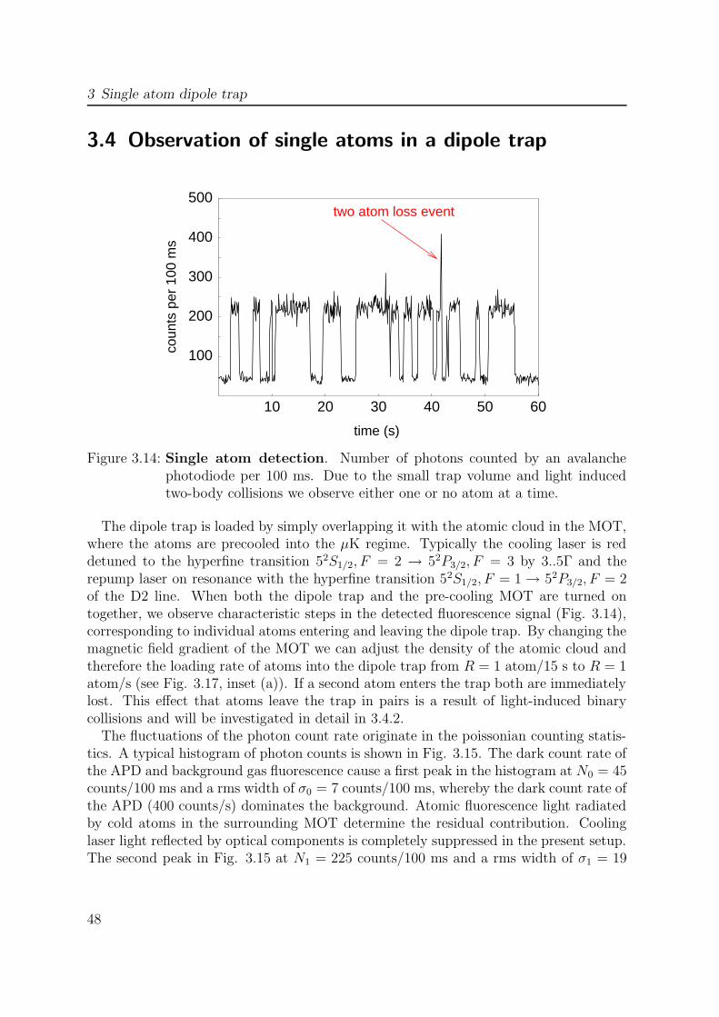
3 Single atom dipole trap
3.4 Observation of single atoms in a dipole trap
10 20 30 40 50 60
100
200
300
400
500
time (s)
coun
ts p
er 1
00 m
s
two atom loss event
Figure 3.14: Single atom detection. Number of photons counted by an avalanchephotodiode per 100 ms. Due to the small trap volume and light inducedtwo-body collisions we observe either one or no atom at a time.
The dipole trap is loaded by simply overlapping it with the atomic cloud in the MOT,where the atoms are precooled into the µK regime. Typically the cooling laser is reddetuned to the hyperfine transition 52S1/2, F = 2 → 52P3/2, F = 3 by 3..5Γ and therepump laser on resonance with the hyperfine transition 52S1/2, F = 1 → 52P3/2, F = 2of the D2 line. When both the dipole trap and the pre-cooling MOT are turned ontogether, we observe characteristic steps in the detected fluorescence signal (Fig. 3.14),corresponding to individual atoms entering and leaving the dipole trap. By changing themagnetic field gradient of the MOT we can adjust the density of the atomic cloud andtherefore the loading rate of atoms into the dipole trap from R = 1 atom/15 s to R = 1atom/s (see Fig. 3.17, inset (a)). If a second atom enters the trap both are immediatelylost. This effect that atoms leave the trap in pairs is a result of light-induced binarycollisions and will be investigated in detail in 3.4.2.
The fluctuations of the photon count rate originate in the poissonian counting statis-tics. A typical histogram of photon counts is shown in Fig. 3.15. The dark count rate ofthe APD and background gas fluorescence cause a first peak in the histogram at N0 = 45counts/100 ms and a rms width of σ0 = 7 counts/100 ms, whereby the dark count rate ofthe APD (400 counts/s) dominates the background. Atomic fluorescence light radiatedby cold atoms in the surrounding MOT determine the residual contribution. Coolinglaser light reflected by optical components is completely suppressed in the present setup.The second peak in Fig. 3.15 at N1 = 225 counts/100 ms and a rms width of σ1 = 19
48

3.4 Observation of single atoms in a dipole trap
100 200 300 400 5000
200
400
600
800
1000
counts per 100 ms
num
ber
of s
ampl
es
Figure 3.15: Single atom detection. Histogram of photon counts per 100 ms of Fig. 3.14.
counts/100 ms is caused by resonance fluorescence of a single atom in the dipole trap.Typical photon counting rates are 500 - 1800 s−1 per atom depending on the detuningand intensity of the cooling laser. For a maximum counting rate of 1800 s−1 per atom wedetermine a minimum time interval of 10 ms to be able to distinguish 1 atom from thebackground counts. As a criterion we require that the difference of count rates of “1”atom and “0” atom, ∆N = N1 −N0, is 4 times larger than the statistical fluctuations ofN1. Provided the fluctuations of the photon count rate are caused only by the poissoniancounting statistics the expected error of this method is 4 percent.
3.4.1 Trap lifetime
The lifetime of single atoms in the dipole trap depends on one hand on collisions withatoms from the background gas, whereby the collision rate is determined by the residualbackground gas pressure in the vacuum chamber. For a gas pressure below 10−10 mbarwe expect a lifetime up to several seconds. On the other hand, this value can dropby many orders of magnitude during the loading stage because light-induced binarycollisions dominate the trap loss.
Depending on the trap depth and the loading rate we observe a mean 1/e lifetimebetween 0.5 and 2.2 s (see Fig. 3.17, inset (b)). Here the lifetime is extracted directlyby histogramming the length of fluorescence steps. Because the cooling and the repumplaser of the MOT are present during the loading stage of the dipole trap, light-inducedtwo-body collisions dominate the trap loss and therefore the measured lifetime.
In a different experiment the characteristic lifetime of single atoms limited only bybackground gas collisions is measured. Therefore, we switch on the cooling and repump
49
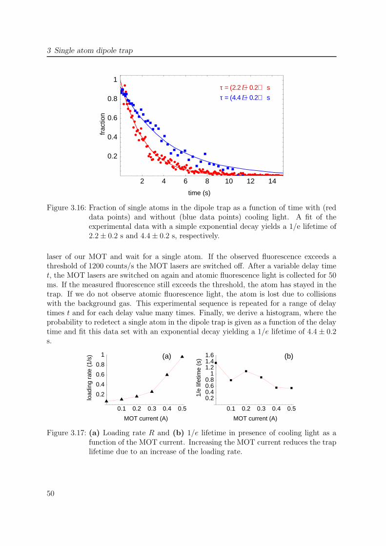
3 Single atom dipole trap
2 4 6 8 10 12 14
0.2
0.4
0.6
0.8
1
time (s)
frac
tion
τ = (2.2 +/− 0.2) s
τ = (4.4 +/− 0.2) s
Figure 3.16: Fraction of single atoms in the dipole trap as a function of time with (reddata points) and without (blue data points) cooling light. A fit of theexperimental data with a simple exponential decay yields a 1/e lifetime of2.2 ± 0.2 s and 4.4 ± 0.2 s, respectively.
laser of our MOT and wait for a single atom. If the observed fluorescence exceeds athreshold of 1200 counts/s the MOT lasers are switched off. After a variable delay timet, the MOT lasers are switched on again and atomic fluorescence light is collected for 50ms. If the measured fluorescence still exceeds the threshold, the atom has stayed in thetrap. If we do not observe atomic fluorescence light, the atom is lost due to collisionswith the background gas. This experimental sequence is repeated for a range of delaytimes t and for each delay value many times. Finally, we derive a histogram, where theprobability to redetect a single atom in the dipole trap is given as a function of the delaytime and fit this data set with an exponential decay yielding a 1/e lifetime of 4.4 ± 0.2s.
0.1 0.2 0.3 0.4 0.5
0.2
0.4
0.6
0.8
1
0.1 0.2 0.3 0.4 0.5
0.20.40.60.8
11.21.41.6
MOT current (A) MOT current (A)
load
ing
rate
(1/
s)
1/e
lifet
ime
(s) (b)(a)
Figure 3.17: (a) Loading rate R and (b) 1/e lifetime in presence of cooling light as afunction of the MOT current. Increasing the MOT current reduces the traplifetime due to an increase of the loading rate.
50

3.4 Observation of single atoms in a dipole trap
3.4.2 Atom number statistics
One important fact concerning the fluorescence detection in our experiment is, thatphoton count rates corresponding to more than one atom never occur up to a maximumMOT current of 0.5 A corresponding to a maximum loading rate of R = 1 s−1. This canbe seen directly from the histogramms of photon counts in Fig. 3.18.
150 300 450 600
50100150200250
n
I = 0.4 A
150 300 450 600
100200300400
n
I = 0.1 A
150 300 450 600
255075
100125150
n
I = 0.5 A
150 300 450 600
100
200
300
n
I = 0.2 A
150 300 450 600
20406080
100n
I = 0.6 A
150 300 450 600
10203040506070
I = 0.7 A
n
150 300 450 600
50100150200250300350
n
I = 0.3 A
150 300 450 600
100200300400
n
I = 0 A
0 0
00
0 0
0 0
counts / 100 ms
counts / 100 ms counts / 100 ms
counts / 100 ms counts / 100 ms
counts / 100 mscounts / 100 ms
counts / 100 ms
Figure 3.18: Histograms of detected photon counts in 100 ms for different MOT currents(I). Up to 0.5 A only single atoms are observed in the dipole trap.
51

3 Single atom dipole trap
0 1 2 3 4 5
0.20.40.60.8
1
0 1 2 3 4 5
0.20.40.60.8
1
0 1 2 3 4 5
0.20.40.60.8
1
0 1 2 3 4 5
0.20.40.60.8
1
0 1 2 3 4 5
0.20.40.60.8
1
0 1 2 3 4 5
0.20.40.60.8
1
R = 0.07 s−1
R = 0.26 s−1 R = 0.60 s−1
R = 0.17 s−1
R = 0.97 s−1
R = 0.11 s−1
Figure 3.19: Measured atom number distributions for different loading rates. Due tothe small dipole trap volume and the presence of light-induced two-bodycollisions during the loading stage the number of trapped atoms is lockedto one up to a loading rate of 1 atom/s.
To compare the measured atom number distributions directly with the calculateddistributions for a trapping beam waist of 3.5µm (see Fig. 3.8), the continuous photoncounting histograms are converted by numerical integration into bar-histograms wherethe probability to load atoms into the dipole trap is plotted as a function of the atomnumber N (see Fig. 3.19). As expected, our measurement results confirm the “blockadeeffect” [73], locking the maximum number of trapped atoms to one.
3.4.3 Temperature measurement of a single atom
In the present experiment a single optically trapped atom is cooled during fluorescencedetection by three-dimensional polarization gradients in an optical molasses. This leadsto a final kinetic energy on the order of 100 µK [70]. Information about the kinetic energycan be gathered by the spectral analysis of the emitted resonance fluorescence, becauseDoppler effects due to the motion in the confining potential lead to a line broadening inthe emitted fluorescence spectrum.
For low excitation intensities the fluorescence spectrum of a two-level atom exhibitsan elastic peak centered at the incident laser frequency ωL, while for higher intensitiesan inelastic component becomes dominant, with contributions at the frequencies ωL andωL ± Ω0 [83], where Ω0 denotes the Rabi frequency. This so so-called “Mollow triplet”arises from the dynamical Stark splitting of the two-level transition and has been ob-served in a number of experiments [84, 85, 86], using low-density atomic beams or asingle trapped and laser-cooled Ba+ ion [87]. Surprisingly, there are only a few exper-imental investigations of the coherent scattering process, with a frequency distributiondetermined by the exciting laser. Subnatural linewidths were demonstrated with atomic
52

3.4 Observation of single atoms in a dipole trap
cooling beams
referencebeam
trappedatom BS
D2
D1
FPI
Figure 3.20: Setup for the measurement of the resonance fluorescence spectrum of lightscattered by a single atom in an optical dipole trap. The fluorescence andexcitation laser light is collected confocally to the trapping beam (see Fig.3.13) and analyzed with a scanning Fabry-Perot Interferometer (FPI). Thereference laser is used to monitor length drifts of the resonator and todetermine the instrumental function of the FPI.
beam experiments [86, 88], atomic clouds in optical molasses [89, 90] and a single trappedand laser-cooled Mg+ ion [91, 92].
For our laser cooling parameters the fluorescence spectrum is dominated by elasticRayleigh scattering [47]. Hence, the emitted fluorescence light exhibits the frequencydistribution of the exciting laser (0.6 MHz FWHM) field broadened by the Doppereffect. Position-dependent atomic transition frequencies in the dipole trap due to theinhomogeneous AC-Stark shift give no additional broadening because the spectrum of theelastically scattered fluorescence light is determined only by the frequency distributionof the exciting light field and not by the atomic transition frequencies.
The resolution achieved with narrow-band Fabry-Perot filter resonators for spectralanalysis is limited to approximately 1 MHz and allows to measure an effective linebroadening on the order of several 10 kHz. This resolution is sufficient to determine thekinetic energy with sufficient accuracy.
Experimental setup
The scattered fluorescence spectrum is analyzed via a scanning Fabry-Perot interfer-ometer (FPI) with a frequency resolution of 0.45 MHz (full width half maximum), atransmission of 40% and a finesse of 370. To measure the spectrum only at times wetrap single atoms, a part of the fluorescence light is monitored separately with a refer-ence APD (D1) (see Fig. 3.20). Since the broadening of the atomic emission spectrumdue to the Doppler effect is expected to be a small effect, the instrumental function of
53

3 Single atom dipole trap
-1 -0.5 0 0.5 10
0.2
0.4
0.6
0.8
1
filter frequency detuning (MHz)
tran
smis
sion
Figure 3.21: Measured spectra of the single atom resonance fluorescence (red datapoints) and the excitation light (blue data points). The spectra exhibita width of 0.94±0.01 MHz and 1.04±0.1 MHz (FWHM) for the excitationand the fluorescence light, respectively. Experimental parameters: ICL = 80mW/cm2, IRL = 12 mW/cm2, ∆CL = −2π × 19 MHz, U = (0.62 ± 0.06)mK.
the spectrometer and the exciting laser line width have to be known accurately. In orderto achieve this, we shine a fraction of the exciting light (reference beam) into the collec-tion optics (see Fig. 3.20). This way, both reference and scattered light are subject tothe identical spectrometer instrumental function whereby the reference laser spectrumis also used to monitor length drifts of the filter cavity. In the experiment the spectrumof the reference beam and the fluorescence light scattered by a single atom in the dipoletrap were recorded alternately. After each measurement a compensation of the cavitydrift was performed by referencing the cavity frequency to the maximum transmissionof the reference laser.
Experimental results
With this procedure we obtained the two (normalized) data sets in Fig. 3.21. Asexpected, the fluorescence spectrum scattered by a single atom exhibits a “subnatu-ral” linewidth of 1.04 ± 0.01 MHz (FWHM) because the elastic Rayleigh contributiondominates the scattering process. The exciting laser light field exhibits a linewidth of0.94 ± 0.01 MHz (FWHM) which is the convolution of the transmission function of theFabry-Perot filter with the spectral width of the excitation laser. The depicted errorbars reflect the statistical error from the individual count rates of each data point. Forthe reference laser this error is too small to be visible in this graph.
For an atom at rest the resonance fluorescence spectrum should show the same linewidth
54
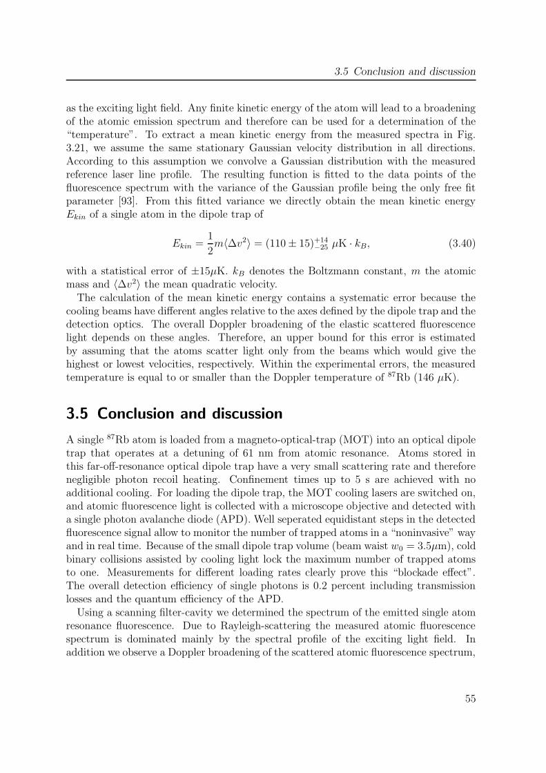
3.5 Conclusion and discussion
as the exciting light field. Any finite kinetic energy of the atom will lead to a broadeningof the atomic emission spectrum and therefore can be used for a determination of the“temperature”. To extract a mean kinetic energy from the measured spectra in Fig.3.21, we assume the same stationary Gaussian velocity distribution in all directions.According to this assumption we convolve a Gaussian distribution with the measuredreference laser line profile. The resulting function is fitted to the data points of thefluorescence spectrum with the variance of the Gaussian profile being the only free fitparameter [93]. From this fitted variance we directly obtain the mean kinetic energyEkin of a single atom in the dipole trap of
Ekin =1
2m〈∆v2〉 = (110 ± 15)+14
−25 µK · kB, (3.40)
with a statistical error of ±15µK. kB denotes the Boltzmann constant, m the atomicmass and 〈∆v2〉 the mean quadratic velocity.
The calculation of the mean kinetic energy contains a systematic error because thecooling beams have different angles relative to the axes defined by the dipole trap and thedetection optics. The overall Doppler broadening of the elastic scattered fluorescencelight depends on these angles. Therefore, an upper bound for this error is estimatedby assuming that the atoms scatter light only from the beams which would give thehighest or lowest velocities, respectively. Within the experimental errors, the measuredtemperature is equal to or smaller than the Doppler temperature of 87Rb (146 µK).
3.5 Conclusion and discussion
A single 87Rb atom is loaded from a magneto-optical-trap (MOT) into an optical dipoletrap that operates at a detuning of 61 nm from atomic resonance. Atoms stored inthis far-off-resonance optical dipole trap have a very small scattering rate and thereforenegligible photon recoil heating. Confinement times up to 5 s are achieved with noadditional cooling. For loading the dipole trap, the MOT cooling lasers are switched on,and atomic fluorescence light is collected with a microscope objective and detected witha single photon avalanche diode (APD). Well seperated equidistant steps in the detectedfluorescence signal allow to monitor the number of trapped atoms in a “noninvasive” wayand in real time. Because of the small dipole trap volume (beam waist w0 = 3.5µm), coldbinary collisions assisted by cooling light lock the maximum number of trapped atomsto one. Measurements for different loading rates clearly prove this “blockade effect”.The overall detection efficiency of single photons is 0.2 percent including transmissionlosses and the quantum efficiency of the APD.
Using a scanning filter-cavity we determined the spectrum of the emitted single atomresonance fluorescence. Due to Rayleigh-scattering the measured atomic fluorescencespectrum is dominated mainly by the spectral profile of the exciting light field. Inaddition we observe a Doppler broadening of the scattered atomic fluorescence spectrum,
55

3 Single atom dipole trap
which allowed us to determine an upper bound of the mean kinetic energy of the trappedatom corresponding a temperature of 110 µK.
56

4 Single photons from single atoms
4.1 Introduction
The experimental results from the previous chapter (see Fig. 3.14) suggest that we ob-serve only single atoms in our dipole trap. This assumption can be verified by a detailedstatistical analysis of the measured stream of photon counts. In particular, nonclassicalfeatures of the resonance fluorescence are observed in the second-order correlation func-tion g(2)(τ), whereby, most prominently, the so-called antibunching behaviour indicatesthe single particle character of the radiating source.
To prove that only a single atom is stored in our trap we have set up a Hanbury-Brown-Twiss (HBT) experiment [94, 95] and studied the statistical properties of thedetected fluorescence light. The measured second-order correlation function exhibitsstrong photon antibunching verifying the presence of a single atom. In addition the two-photon correlations show the internal quantum dynamics of the population occupationof the atomic hyperfine levels involved in the excitation process, whereby the observedoscillations can be explained with a four-level model. To compare the theoretical modelwith the experimental data we numerically solve optical Bloch equations and calculatethe second order correlation function of the emitted fluorescence light. We find goodagreement with the measured data.
Due to the complex structure of photon-pair correlations which depend on the internaland external dynamics of the atom-light interaction, I will first introduce theoreticalaspects relevant for the understanding of the present experiment before I will discussmeasured experimental data.
4.2 Theoretical framework
4.2.1 Second-order correlation function
For the scattered light field of atomic resonance fluorescence described by the electricfield operators E+ and E−, the two-photon correlation function g2(τ) is given, accordingto Glauber [96] (see also [97]), by
g(2)(τ) =〈E−(t)E−(t+ τ)E+(t+ τ)E+(t)〉
〈E−(t)E+(t)〉2, (4.1)
57

4 Single photons from single atoms
where τ ≥ 0. For almost monochromatic light fields and a small detection probability,this function is the conditional probability of detecting a photon at time t+ τ , given theprevious detection of another photon at time t, normalized by the factorized value forstatistically independent photons. Whereas classical fields show correlation functionsg(2)(0) ≥ 1 and g(2)(τ) ≤ g(2)(0), the nonclassical resonance fluorescence of a single atomexhibits the so-called antibunching behaviour, i.e., g(2)(0) = 0 and g(2)(τ) > g(2)(0). Thiscondition signals sub-Poissonian emission probability.
4.2.2 Two-level atom
The resonance scattering from an atom can be described by the electromagnetic fieldoperators in the Heisenberg picture. For a two-level atom at position R with a dipoletransition, the electric field operator E+(r, t) at a point r is given in the far-field regionby
E+(r, t) = E+free(r, t) + E+
S (r, t), (4.2)
where E+free(r, t) is the field unperturbed by the atom. This part contains the vacuum
fluctuations and the externally applied (laser) light. The point of detection r is chosensuch that the excitation light field is negligible and therefore the freely-propagating partcan be dropped. The second contribution in Eq. (4.2) is the source field part E+
S (r, t)which represents the field scattered by the atom. It is given by [97]
E+S (r, t) = −ω
20|〈g|d|e〉| sin θ4πε0c2|r − R| ~εSπ(t− |r− R|
c). (4.3)
Here, ω0 is the angular frequency of the atomic transition |g〉 → |e〉, 〈g|d|e〉 is thecorresponding dipole matrix element, and R is the center-of-mass coordinate of theatom. The operator π(r, t) contains the spatio-temporal dependence of the light fieldand is defined by π = |g〉〈e|. For the negative part of the electric field the correspondingoperator is defined by π† = |e〉〈g| respectively. The angle θ is subtended between thedipole matrix element and the direction of observation, r − R. The linear polarizationof the emitted field, ~εS, is in the plane perpendicular to the direction of observation, andparallel to the projection of the dipole matrix element into this plane.
The coherence properties of the light emitted by a single two-level atom in free spacecan now be calculated with the use of the source-field expression (4.3), and we get forthe second-order correlation function of the emitted fluorescence light
g(2)(τ) =〈π†(t)π†(t+ τ)π(t+ τ)π(t)〉
〈π†(t)π(t)〉2 , (4.4)
where the time delay τ is always positive. This relation contains the expectation valueof two observables at different times. With the help of the quantum regression theorem[98] the two-time expectation values can be reduced to particular one-time expectation
58

4.2 Theoretical framework
g(2
)(τ
)
2 4 6 8 10
0.250.5
0.751
1.251.5
1.752
Γ ∗ τ
∆ = 0
Figure 4.1: Second-order correlation function g(2)(τ) of a two-level atom versus the di-mensionless delay time Γτ for ΩR/Γ = 4 (green solid line) and ΩR/Γ = 0.4(red dashed line, respectively).
values. Performing some calculations [49], the second-order correlation function is foundto be:
g(2)(τ) =ρee(τ)
ρee(∞). (4.5)
Here ρee(τ) is the element of the atom’s density matrix that represents the populationof the excited atomic state at the time τ . This element can be calculated from opticalBloch equations (OBE) [80] with the initial conditions ρee(0) = ρeg(0) = ρge(0) = 0,and ρgg(0) = 1, which describe the state of the atom immediately after the emission ofa photon. The theoretically predicted correlation function is given by [99]
g(2)(τ) = 1 − e−3Γτ/4[cos(ΩRτ) +3Γ
4ΩRsin(ΩRτ)], (4.6)
where Ω2R = Ω2
0 + ∆2 − (Γ/4)2, with the Rabi frequency Ω0 at resonance, the naturallinewidth Γ, and the detuning ∆.
In Fig. 4.1, the second-order correlation function is plotted as a function of the timedelay τ for different values of the generalized Rabi frequency ΩR of the driving field.For τ = 0 the two-photon correlation function g(2)(τ) = 0, which corresponds to thephenomenon of photon antibunching. Once a photon is emitted, the atom is foundin the ground state and it takes the driving field some time to reexcite the atom tothe upper level, from which the next photon can be emitted. On average, this delayis of the order of the Rabi period Ω−1
R . For a weak driving field, ΩR/Γ < 1, g(2)(τ)increases monotonically from 0 to 1 as τ is increased. For a strong driving field, ΩR/Γ >1, i.e. the generalized Rabi frequency ΩR and thus the frequency of populating and
59

4 Single photons from single atoms
depopulating the excited state is greater than the decay rate Γ. Therefore g(2)(τ) showsan oscillatory dependence on τ . The magnitude of these oscillations decreases as τ isincreased and g(2)(τ) approaches unity as τ → ∞. The upper limit of g(2)(τ) for theresonance fluorescence of a two-level atom is 2.
Both antibunching and sub-Poissonian statistics in resonance fluorescence have beenobserved in quantum optical experiments with atoms [100, 101]; however corrections forthe fluctuating atom numbers in the atomic beam had to be taken into account. Witha single trapped Mg+ ion Diedrich et al. [102] observed antibunching of an individualtwo-level atom. In that experiment antibunching in the resonance fluorescence of one,two, and three trapped ions was observed and the antibunching property decreased aspredicted for increasing ion numbers, since for an increasing number of independentatoms the photon counts become more and more uncorrelated.
Aside from antibunching and sub-Poissonian statistics, Schubert et al. [103] observedtwo-photon correlations in the resonance fluorescence of a single Ba+ ion with a max-imum much larger than what is possible with two-level atoms, as well as photon an-tibunching with much larger time constants of the initial photon anticorrelation. Adetailed study of the internal eight-level dynamics on the basis of optical Bloch equa-tions allowed a quantitative description of the observed g(2)(τ) functions [104].
4.2.3 Four-level model
For the fluorescence detection of a single atom in the dipole trap we use the MOTcooling laser (CL) red detuned to the unperturbed hyperfine transition 52S1/2, F = 2 →52P3/2, F = 3 (Fig. 4.2) by ∆ = 4..5Γ. To avoid optical pumping to the hyperfine groundlevel F = 1 during the loading process we additionally shine in a repump laser (RL) onresonance with the hyperfine transition 52S1/2, F = 1 → 52S1/2, F
′ = 2. Because theatom is stored in a dipole trap, the AC Stark-effect additionally shifts the cooling andrepump laser to the red of resonance and leads to significant optical pumping to F = 1.Hence, we expect a more detailed multi-level model - which includes also this pumpingeffect - to correctly describe the internal dynamics of the atom-light interaction.
In general it is quite complicated to describe the situation of a laser-cooled single atomin a dipole trap, because the six counter-propagating circularly polarized cooling laserbeams of the MOT form an intensity lattice in space and a discrete set of points withzero intensity. The form of this interference pattern is specific to the set of phases chosen.Due to the finite kinetic energy corresponding to a temperature of approximately 110µK (see preceding chapter) the atom oscillates in a classical picture with an amplitudecorresponding to several optical wavelengths. During this oscillatory movement theatom experiences both a changing intensity and polarization. This situation suggests tosimplify the internal atomic dynamics neglecting the Zeeman substructure of the involvedhyperfine levels and to treat the exciting cooling and repump light as two unpolarizedlaser fields with an average intensity of six times the single beam intensity.
60

4.2 Theoretical framework
abΓ
Γdc
d
a
2 P3/2
2 S1/2c
b
CL
RL
Γac
F=2
F=1
F’=2
F’=3
ω
ω
∆
Figure 4.2: Effective level structure in 87Rb used for fluorescence detection. The coolinglaser field (CL) couples F = 2 → F ′ = 3 and F = 2 → F ′ = 2, whereas therepump laser field (RL) couples only F = 1 → F ′ = 2.
Optical Bloch equations
In the following I will focus on an atomic four-level system as indicated in Fig. 4.2 andthe interaction with two classical light fields. The Hamiltonian H of the system reads
H = H0 +Hint, (4.7)
where H0 denotes the Hamiltonian of the free atom and Hint the interaction with therepump laser field ERL of angular frequency ωRL and the cooling laser field ECL ofangular frequency ωCL respectively.
The equation of motion for the atomic density matrix ρ of the system is given by
ρ =−ih
[H, ρ] +R, (4.8)
where the brackets [ , ] are defined by [H, ρ] = Hρ − ρH and the relaxation term Rrepresents the spontaneous decay process. In the rotating-wave approximation (RWA)we obtain for the HamiltonianH the matrix representation in the basis of the bare atomicstates |a〉, |b〉, |c〉 and |d〉 corresponding to the hyperfine states |F ′ = 2〉, |F = 1〉, |F = 2〉and |F ′ = 3〉:
H = h
ωa −Ω1
2e−iωRLt −Ω2
2e−iωCLt 0
−Ω1
2eiωRLt ωb 0 0
−Ω2
2eiωCLt 0 ωc −Ω3
2eiωCLt
0 0 −Ω3
2e−iωCLt ωd
. (4.9)
We assume the repump laser to excite the F ′ = 2 level, whereas the cooling laser excitesboth hyperfine levels F ′ = 2 and F ′ = 3. The strength of these couplings are described
61

4 Single photons from single atoms
by the on-resonance Rabi frequencies Ω1, Ω2 and Ω3 respectively. They are defined by
Ω1 = Γ
√
IRL2I12
s
, Ω2 = Γ
√
ICL2I22
s
and Ω3 = Γ
√
ICL2I23
s
, (4.10)
where Γ = 2π × 6 × 106 Hz is the decay rate of the transition 52S1/2 → 52P3/2. For anisotropic excitation light field (i.e. a pumping field with equal components in all threepossible polarizations) the saturation intensities of the hyperfine transitions F = 1 →F ′ = 2, F = 2 → F ′ = 2 and F = 2 → F ′ = 3 can be calculated [61] to I12
s = 6.01mW/cm2, I22
s = 10.01 mW/cm2 and I23s = 3.58 mW/cm2. ICL and IRL denote the
intensities of the cooling and repump laser, respectively.The relaxation term R in the master equation represents spontaneous decay [105, 59]
from the excited hyperfine levels a and d. In matrix representation we obtain
R =
−(Γab + Γac)ρaa −γabρab −γacρac 0−γabρba Γabρaa 0 0−γacρca 0 Γacρaa + Γdcρdd −γdcρcd
0 0 −γdcρdc −Γdcρdd
, (4.11)
where Γab, Γac, and Γdc are the energy and γab, γac, and γdc are the respective phaserelaxation rates. Energy relaxation from c→ b is neglected.
The energy relaxation rates appear in the diagonal elements of R and describe popu-lation loss of all involved levels due to spontaneous emission. In detail, Γdc is given bythe spontaneous emission rate Γ of the 2P3/2 excited state in 87Rb, whereas Γac and Γabrefer to spontaneous decay from a → c and a → b. The ratio of Γab/Γac is given by thebranching ratio of the respective hyperfine transitions and obeys the relation
Γ = Γac + Γab. (4.12)
In the case of an isotropically polarized excitation light field the respective branchingratio is 1/2. Population loss acts also on the nondiagonal matrix elements of R. Ingeneral, the phase relaxation rate of a transition n→ m is given by [59]
γnm =1
2(Γn + Γm), (4.13)
where Γn denotes the sum of any population loss of level n, and Γm of m respectively.In our case the phase relaxation rates are given by
γab =1
2(Γab + Γac), γac =
1
2(Γab + Γac), and γdc =
1
2Γdc. (4.14)
From Eq. (4.8) we derive optical Bloch equations (OBE) for the four-level system asshown in Fig. 4.2. As this set of 16 coupled ordinary differential equations entails nonew physics, they are not shown explicitly.
62

4.2 Theoretical framework
To solve the OBE by numerical integration [106] it is convenient to suppress anyexplicit time dependence in the coefficients of the OBE. Hence we introduce new variablesρik (i, k = a, b, c, d) which are given in matrix representation by
ρ =
ρaa ρabeiωRLt ρace
iωCLt ρadρbae
−iωRLt ρbb ρbce−i(ωRL−ωCL)t ρbde
−iωRLt
ρcae−iωCLt ρcbe
i(ωRP −ωCL)t ρcc ρcde−iωCLt
ρda ρdbeiωRLt ρdce
iωCLt ρdd
. (4.15)
Photon correlation function
The photon correlation function as defined in Eq. (4.1) is a two-time expectation valueof the electric field operators E− and E+ of the scattered light field. Hence, features ofthe photon correlation function originate from the structure of E. For the present caseof a four-level atom Eq. (4.2) can be generalized by assuming that each dipole transitionof the atom contributes to the field a term like E+
S in Eq. (4.3). With the help of thequantum regression theorem [98] the resulting correlation function is given by
g(2)(τ) =ρaa(τ) + ρdd(τ)
ρaa(∞) + ρdd(∞), (4.16)
the ratio of the excited state populations at time τ and in the steady state (τ = ∞).To evaluate this expression, the optical Bloch equations have to be solved for bothsteady-state and time-dependent cases.
The time-dependent solution depends on the initial conditions for the density matrix,and it is this point where different correlation functions can be distinguished [104].Physically, the initial conditions describe the state of the atom after the emission ofthe first photon and consequently depend on the properties of that photon. Thus thecorrelation function depends on the wavelength of the first photon, but does not dependon the properties of the second photon.
In the HBT experiment performed (see next section) we do not distinguish from whichtransition the first photon came from. In this case the initial conditions for the numericalcalculation of the density matrix elements ρaa(τ) and ρdd(τ) can be determined from thesteady-state solution. All matrix elements vanish, ρij(0) = 0, except
ρbb(0) =Γabρaa(∞)
(Γab + Γac)ρaa(∞) + Γdcρdd(∞)and (4.17)
ρcc(0) =Γacρaa(∞) + Γdcρdd(∞)
(Γab + Γac)ρaa(∞) + Γdcρdd(∞). (4.18)
These initial conditions characterize the state of the atom immediately after the emissionof any photon: the atom is in the 2S1/2 levels |b〉 and |c〉, whose relative population isgiven by the probabilities for spontaneous emission on the transitions |a〉 → |b〉, |a〉 → |c〉and |d〉 → |c〉.
63

4 Single photons from single atoms
Following the described procedure we calculated the second-order correlation functiong(2)(τ) for different detunings ∆ of the cooling laser (see Fig. 4.3). The repump laseris supposed to be on resonance. Increasing ∆ leads to significant optical pumping tothe F = 1 hyperfine ground level and to a breakdown of the two-level model. Todemonstrate this effect, we calculated the photon correlation function for a two-leveland four-level model for equal experimental parameters. For small detunings of thecooling laser, the second-order correlation functions based on a two-level and four-levelmodel are indistinguishable.
g(2
)(τ
)g
(2)
(τ)
g(2
)(τ
)
2 4 6 8 10
1
2
3
4
5
2 4 6 8 10
1
2
3
4
5
2 4 6 8 10
1
2
3
4
5
2 4 6 8 10
1
2
3
4
5
2 4 6 8 10
2
4
6
8
2 4 6 8 10
2
4
6
8
Γ ∗ τ
Γ ∗ τ
Γ ∗ τ
∆ = − Γ ∆ = − 5Γ
∆ = − 10Γ ∆ = − 15Γ
∆ = − 20Γ ∆ = − 25Γ
Γ ∗ τ
Γ ∗ τ
Γ ∗ τ
Figure 4.3: Calculated intensity correlation function g(2)(τ) for different detunings ∆ ofthe cooling laser. Blue line: two-level model; red line: four-level model.Experimental parameters: ICL = 100 mW/cm2, IRL = 12 mW/cm2
64

4.2 Theoretical framework
For larger detunings, corresponding to the situation of a single 87Rb atom in a MOTor an optical dipole trap (∆ = −5.. − 10Γ), the photon-pair correlation function ofthe four-level model shows deviations from the predictions of a simple two-level model.Most prominently the amplitudes of the Rabi oscillations exceed the upper limit of 2,which is predicted by a two-level model. Increasing the detuning of CL further increasesthe coupling to the level |a〉. Hence, the multi-level structure becomes more and moredominant. On the one hand this gives rise to several generalized Rabi frequencies, onthe other hand to significant optical pumping to F=1. For large detunings of the coolinglaser (∆ > −20Γ) the envelope of the correlation function shows the predicted featureof a three-level Λ-type atom [107]. The calculated correlation functions in Fig. 4.3demonstrate this behavior very well.
4.2.4 Motional effects
Since the correlation function of the emitted light depends on the incident field, themotion of the atom will modify the photon correlations. Moving through the dipole trapthe atom crosses various spots of a light interference pattern with different intensity andpolarization. In our experiment this interference pattern is formed by the intersectionof three pairs of counterpropagating σ+-σ− polarized laser beams used for laser coolingand fluorescence detection. The polarization of resonance fluorescence is determined bythe magnetic orientation of the atom, which in turn depends on the local light fieldand changes on the time scale of atomic motion over an optical wavelength λ. Thus, inaddition to correlations of the total intensity (4.1) one expects polarization effects to bevisible in two-photon correlations [108].
Our measurements of the photon statistics are only sensitive to total intensity cor-relations caused by a standing light field pattern. Hence, I will restrict the followingtheoretical considerations only to total intensity correlations. Because of the entangle-ment of internal and external degrees of freedom, a proper description of the atomicdynamics is a non-trivial problem [109, 110]. I do not intend here to present a sophis-ticated theory but rather to describe the atomic motion in a simple phenomenologicalway.
Fokker-Planck equation
The trapping force in a dipole trap with a superimposed 1D σ+-σ− polarization gradientcooling includes two partial forces, i.e., the gradient force of the dipole potential (see Eq.3.4) and the radiation pressure force [70] and can be expressed as a damped harmonicoscillation with spring constant κ and friction parameter α. In a simple model randomfluctuations of the friction force may be characterized by a diffusion constant D =kBT/α, where T is the temperature (which has the meaning of an average kinetic energyof the trapped atom) and kB denotes the Boltzmann constant. Treating the dipolepotential as an effective harmonic potential, the theory of Brownian motion [80] can be
65

4 Single photons from single atoms
used to derive a Fokker-Planck equation for the atomic motion:
∂
∂tf =
κ
α
∂
∂z(zf) +
kT
α
∂2
∂z2f. (4.19)
Here the function f = f(z, z0, t) describes the probability density for the atom to be attime t at position z for the initial atomic position z(t = 0) = z0.
For atomic motion in potential-free space (situation in an optical molasses), theFokker-Planck equation reduces to a diffusion equation
∂
∂tf = D
∂2
∂z2f. (4.20)
The probability function f which solves this differential equation has the form
f(z, z0, t) =1√
2πσ(t)e− (z−z0)2
2σ2(t) , (4.21)
where σ(t) =√
2Dt describes the temporal spread of the atomic positional probability,which is an expanding Gauss if there is no potential.
Total intensity correlation function
In order to gain physical insight how the diffusive motion of a single atom in an intensitymodulated standing light field will influence the total intensity correlation function, Iwill start with an atom modeled by a classical emitter with an induced dipole momentproportional to the local light field. Then the corresponding total correlation functionis given by
g(2)tot (τ) =
∫ ∫∞−∞ I(z0)I(z)f(z0, z0,∞)f(z, z0, τ)dzdz0
〈I(t)〉2 , (4.22)
where the position dependent fluorescence intensity is given by I(z) and the probabilitydensity for the atom to be at time t at z, if its initial position was z(t = 0) = z0, isf(z, z0, t).
Let’s assume that the atom moves “diffusively” in potential-free space in a one-dimensional light field configuration, produced by two plane waves counterpropagat-ing along z with the same frequency, equal amplitudes and equal linear polarizations(I(z) ∝ cos2(kz)). Then the total second-order correlation function g
(2)tot (τ) of the emit-
ted fluorescence light is given by [108]
g(2)tot (τ) = 1 +
1
2e−2k2σ2(τ). (4.23)
This correlation function contains information on the character of the atomic motion.For instance, diffusion (σ ∝
√t) is indicated by an exponential decay whereas ballistic
66

4.3 Experimental determination of the photon statistics
motion (σ ∝ t) yields a Gaussian decay. All correlations vanish after the atom hasmoved more than a distance of λ/2. The corresponding decay time constant τ0 is thengiven by
τ0 =1
4k2D, (4.24)
where k = 2π/λ. As the diffusion constant D depends on the atomic temperature Tand the friction parameter α, the preceding relation allows to determine the atomictemperature provided the friction parameter was calculated [70] or measured.
4.3 Experimental determination of the photon statistics
4.3.1 Setup
The correlation function g(2)(τ) of the collected fluorescence light is measured in a stan-dard Hanbury-Brown-Twiss configuration with two single photon detectors (D1 and D2)behind a beam splitter (BS, Fig. 4.4). To suppress cross talk in the optical setup, infrontof each detector we insert a bandpass filter (IF) blocking unwanted fluorescence lightcaused by the breackdown flash of the other silicon avalanche photo diode which followsthe detection of a photon [111]. The differences of detection times τ = t1 − t2 of photonpair events are then recorded in a storage oscilloscope with a time resolution of 100 ps.However, the minimum bandwidth of the measurements is limited by the 1.4 ns timingjitter of the detectors.
The normalized distribution of time differences τ is equivalent to the second ordercorrelation function g(2)(τ) as long as τ is much smaller than the mean time differencebetween two detection events [112]. For correct normalization of the measured g(2)(τ)we divide the coincidences in each time bin ∆τ by r1 × r2 × ∆τ × Tint, where r1 andr2 are the mean count rates of the two detectors, and Tint is the total integration timewith an atom in the trap.
IF
IF
optics
t
BS
D2
D1
oscilloscope
from detection
1
t 2
Figure 4.4: Hanbury-Brown-Twiss setup to measure the photon pair correlation functiong(2)(τ). The fluorescence light is sent through a beam splitter BS onto twosingle photon detectors D1, D2 to record detection time differences τ = t1−t2.
67

4 Single photons from single atoms
-50 0 50 100
1
2
3
4
0 2 4 6 8 10
0.8
1
1.2
1.4
1.6
1.8
2 (a)
(b)
g(2
)(τ
)g
(2)
(τ)
τ (µs)
τ (ns)
Figure 4.5: Second-order correlation function g(2)(τ) of the resonance fluorescence of asingle 87Rb atom. (a) On long timescales, g(2)(τ) shows a monotonous decayfor | τ |≤ 2..3µs. (b) On short timescales, clear photon anti-bunching atτ = 0 and oscillations due to Rabi flopping are observed. The red dashed lineindicates accidental coincidences due to the dark count rate of the detectors.Experimental parameters: ICL = 103 mW/cm2, IRL = 12 mW/cm2, ∆/2π =−31 MHz, U = 0.38 mK.
68

4.3 Experimental determination of the photon statistics
4.3.2 Experimental results
In a first experiment we measured the second-order correlation function of the lightcollected from the center of our dipole trap potential in the continous loading mode ofthe trap (cooling and repump lasers are present during the whole measurement time). Inthis operating regime we observe characteristic steps in the detected fluorescence signal(see Fig. 3.14). To minimize background contributions, photon correlations are acquiredonly at times we observe fluorescence exceeding a threshold of 1200 counts per second(cps), i.e. when an atom was inside the trap.
Fig. 4.5 shows the resulting correlation function g(2)(τ) for a dipole potential ofU = 0.38 ± 0.04 mK, a total cooling laser intensity ICL ≈ 103mW/cm2 and detuning∆/2π of -31 MHz respectively. On a µs timescale the correlation function shows anexponential decay from the asymptotic value 1.24 at τ = 0 to 1.0 for large τ with atime constant of 1.8 µs. This decay is caused by the fluorescence of an atom undergoingdiffusive motion in the intensity-modulated light field of the cooling beam configuration(see 4.2.4).
On short timescales, most prominently the uncorrected minimum value g(2)(0) =0.52 ± 0.14 at zero delay τ = 0 clearly proves photon anti-bunching of the emittedfluorescence. Including accidental coincidences due to a dark count rate of 300 s−1
of each detector (dashed red line in Fig. 4.5), we derive a corrected minimum valueg(2)corr(τ = 0) = 0.02 ± 0.14. Within our experimental errors this is compatible with
perfect photon anti-bunching verifying the presence of only one single atom in the dipoletrap. Furthermore, the signature of Rabi-oscillations is observed due to the coherentinteraction of the cooling and repump laser fields with atomic hyperfine levels involvedin the excitation process. The oscillation frequency is in good agreement with thesimple two-level model [99] and the oscillation amplitude is damped out on the expectedtimescale of the 52P3/2 excited state lifetime. Increasing the dipole laser power from 16.7mW to 35.5 mW without changing the laser cooling parameters increases the detuningof the cooling laser to the hyperfine transition 52S1/2(F = 2) → 52P3/2(F
′ = 3) due toan increase of the AC Stark-shift of the atomic levels in the dipole trap laser field. Thiseffect was observed as the expected increase of the oscillation frequency from 47.5 MHzto 62.5 MHz (see Fig. 4.7).
In contrast to a two-level atom, the measured and background corrected correlationsin Fig. 4.7(b) show a maximum value of 6 close to τ = 0. This increase of the oscillationamplitude is a consequence of the atomic multi-level structure and can be explained verywell by the four-level model presented in the theory section of this chapter.
For a detailed interpretation of the measured g(2)(τ) functions on a short timescalewe calculated g(2)(τ) on the base of the four-level model for given experimental param-eters and multiplied it with the function 1 + Ae−τ/τ0 , describing the additional decaycontribution due to motion in the intensity modulated light field of the cooling beamconfiguration. The parameters A and τ0 we determined from an extra fit to the back-ground corrected correlation function on the µs time scale (see Fig. 4.6). The light-shift
69

4 Single photons from single atoms
2 4 6 8 10
0.6
0.8
1
1.2
1.4
1.6
1.8
2
g(2
) (τ)
τ (µs)
τ = 1.8 µs0
Figure 4.6: Background corrected second-order correlation function g(2)(τ) in the reso-nance fluorescence of a single atom in the dipole trap and fit with model-function (4.23). Experimental parameters: ICL = 103 mW/cm2, IRL = 12mW/cm2, ∆/2π = −31 MHz, U = 0.38 mK.
of the atomic hyperfine levels is calculated on the basis of Eq. 3.23 for both the groundlevels F = 1 and F = 2 as well as the relevant hyperfine levels F ′ = 2 and F ′ = 3of the 52P3/2 state and included into the four-level model. Furthermore a reduction ofthe light-shift potential is incorporated in the calculations due to a finite kinetic energyof the atom of approximately 100 µK. For two different depths of the optical trappingpotential we find good agreement of the measured second order correlation function g(2)
τ
with the calculated one (see Fig. 4.6).
4.4 Conclusion and discussion
To prove that only single atoms are stored in our dipole trap, the statistical propertiesof the detected fluorescence light were studied with a Hanbury-Brown-Twiss setup. Themeasured second-order correlation function g(2)(τ) of the detected fluorescence lightexhibits strong photon antibunching verifying the presence of a single atom. In additionthe measured two-photon correlations show the internal and external dynamics of theatomic hyperfine levels involved in the excitation process. Due to the AC Stark-shift ofthe atomic levels in the dipole potential and the resulting increase of the detuning of thecooling light, significant population is continuously transferred to the second hyperfineground state 52S1/2, F = 1. Thus the atom-light interaction can not be modeled with asimple two-level model. An atomic four-level model is developed and its predictions arecompared with measured experimental data. Within our experimental errors we find
70
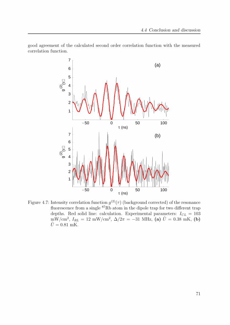
4.4 Conclusion and discussion
good agreement of the calculated second order correlation function with the measuredcorrelation function.
-50 0 50 100
1
2
3
4
5
6
7
-50 0 50 100
1
2
3
4
5
6
7(a)
(b)
τ (ns)
τ (ns)
g(2
) (τ)
g(2
) (τ)
Figure 4.7: Intensity correlation function g(2)(τ) (background corrected) of the resonancefluorescence from a single 87Rb atom in the dipole trap for two different trapdepths. Red solid line: calculation. Experimental parameters: ICL = 103mW/cm2, IRL = 12 mW/cm2, ∆/2π = −31 MHz, (a) U = 0.38 mK, (b)U = 0.81 mK.
71

5 Detection of atomic superposition
states
5.1 Introduction
To verify entanglement between the spin state of a single atom and the polarization of aspontaneously emitted photon, one has to perform correlated local measurements of theinternal quantum states of the atom and the photon. The polarization state of a singlephoton can be measured relatively simply by a combination of a polarization filter anda single photon detector. However, the measurement of the spin state of a single atomis not trivial and therefore the primary experimental challenge of the present work.
In experiments with trapped ions, the state of an atomic qubit encoded in the internalatomic level structure can be measured with almost perfect detection efficiency on thebasis of the “electron shelving” method [113]. This technique has the relevant propertythat depending on the internal quantum state, the atom scatters fluorescence light froman incident laser light field. Hence, the presence or absence of atomic fluorescence lightindicates directly the quantum state of the atom.
In this chapter I will show how the experimental techniques of coherent populationtrapping (CPT) and stimulated Raman adiabatic passage (STIRAP) can be used forphase-sensitive probing of coherent superposition states of a single atom. Therefore Iwill first give a short theoretical review on coherent population trapping and adiabaticpopulation transfer in three- and four-level systems, before I present experiments thatallow to detect a single Rubidium 87 atom in a coherent superposition |mF = −1〉 +eiφ|mF = +1〉 of the Zeeman sublevels mF = ±1 of the hyperfine ground state 2S1/2,F = 1.
5.2 Theoretical framework
Atomic states that do not couple to an incident light field are called dark states andare used in the present work in various ways to prepare and analyze atomic states. Ingeneral one can distinguish three kinds of dark states. (1) The atom is in a state thatcan couple to a light field due to selection rules of electromagnetic dipole transitions.But the incident light field is detuned far-off-resonance and therefore couples negligiblyto the incident light. (2) The atom is in a state that can not couple to a light field due toatomic selection rules. (3) The atom is in a coherent superposition of two ground states
72
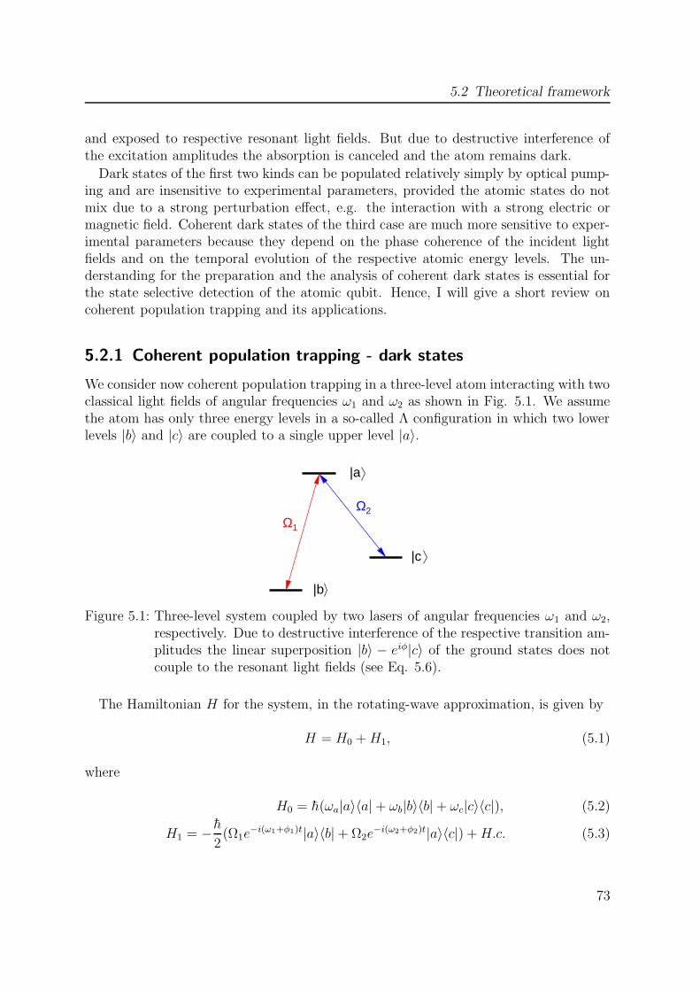
5.2 Theoretical framework
and exposed to respective resonant light fields. But due to destructive interference ofthe excitation amplitudes the absorption is canceled and the atom remains dark.
Dark states of the first two kinds can be populated relatively simply by optical pump-ing and are insensitive to experimental parameters, provided the atomic states do notmix due to a strong perturbation effect, e.g. the interaction with a strong electric ormagnetic field. Coherent dark states of the third case are much more sensitive to exper-imental parameters because they depend on the phase coherence of the incident lightfields and on the temporal evolution of the respective atomic energy levels. The un-derstanding for the preparation and the analysis of coherent dark states is essential forthe state selective detection of the atomic qubit. Hence, I will give a short review oncoherent population trapping and its applications.
5.2.1 Coherent population trapping - dark states
We consider now coherent population trapping in a three-level atom interacting with twoclassical light fields of angular frequencies ω1 and ω2 as shown in Fig. 5.1. We assumethe atom has only three energy levels in a so-called Λ configuration in which two lowerlevels |b〉 and |c〉 are coupled to a single upper level |a〉.
|b
|c
|a
Ω1
Ω2
Figure 5.1: Three-level system coupled by two lasers of angular frequencies ω1 and ω2,respectively. Due to destructive interference of the respective transition am-plitudes the linear superposition |b〉 − eiφ|c〉 of the ground states does notcouple to the resonant light fields (see Eq. 5.6).
The Hamiltonian H for the system, in the rotating-wave approximation, is given by
H = H0 +H1, (5.1)
where
H0 = h(ωa|a〉〈a| + ωb|b〉〈b| + ωc|c〉〈c|), (5.2)
H1 = − h2(Ω1e
−i(ω1+φ1)t|a〉〈b| + Ω2e−i(ω2+φ2)t|a〉〈c|) +H.c. (5.3)
73

5 Detection of atomic superposition states
Ω2 Ω1
time
Rab
i fre
quen
cy
Figure 5.2: Time dependence of the Rabi frequencies required for efficient populationtransfer from the initial state |b〉 to the final state |c〉 under adiabatic follow-ing conditions [114].
Here Ω1 exp (−iφ1) and Ω2 exp (−iφ2) are the Rabi frequencies associated with the cou-pling of the field modes to the atomic transitions |a〉 → |b〉 and |a〉 → |c〉, respectively.The atomic wave function of the system can be written in the form
|ψ(t)〉 = ca(t)e−iωat|a〉 + cb(t)e
−iωbt|b〉 + cc(t)e−iωct|c〉, (5.4)
where the ci(t) are the complex amplitudes of the respective atomic basis states |i〉. Itsdynamics is governed by the time-dependent Schrodinger equation ih|ψ(t)〉 = H|ψ(t)〉.
We now assume the initial atomic state to be a superposition of the two lower levels|b〉 and |c〉
|ψ(0)〉 = cos θ|b〉 + sin θe−iψ|c〉. (5.5)
For Ω1 = Ω2, θ = π/4, and φ1 − φ2 − ψ = ±π it can be verified [49] that
|ψd(0)〉 =1√2(|b〉 − eiφ|c〉) (5.6)
is one of three eigenstates of the Hamiltonian H, whereby the phase φ = φ1 − φ2 isgiven by the phase difference between Ω1 and Ω2. The mentioned eigenstate has a zeroeigenvalue and it is the only eigenstate which does not include a contribution of theexcited level |a〉. Due to destructive interference of the transition amplitudes the atomicpopulation is trapped in a coherent superposition of the lower states and there is noabsorption or scattering even in the presence of resonant light fields. So this state iscalled “dark”. However, the orthogonal state |b〉 + eiφ|c〉 couples to the incident lightfields Ω1 and Ω2 because of constructive interference of Ω1 and Ω2. Hence, this state iscalled “bright”.
5.2.2 Stimulated Raman adiabatic passage
An interesting and powerful application of coherent population trapping in three-stateatoms is the transfer of population with a counter-intuitive sequence of pulses [115]. This
74

5.2 Theoretical framework
technique called stimulated Raman adiabatic passage (STIRAP) allows, in principle, acomplete coherent population transfer from a single initial to a single final quantumstate [115, 114, 116, 117, 118, 119]. The underlying physical mechanism is the existenceof an adiabatically decoupled (or dark) state, which at early and late times coincideswith the initial and target quantum state respectively. This process is robust againstmoderate variations of the pulse form, area and delay between the pulses and thereforeis well suited for experimental applications.
Consider again the three-level system in Fig. 5.1. Provided we start at t = 0 withthe atom in state |b〉 and Ω1 = 0 with Ω2 finite and then proceed to turn Ω2 off whileadiabatically turning Ω1 on (see Fig.5.2), we will end up with the atom in the state |c〉.This is made clear by realizing that the atom is in the time-dependent dark state [114]
|ψd(t)〉 = cos θ(t)|b〉 − sin θ(t)eiφ|c〉, (5.7)
where
tan θ(t) =Ω1(t)
Ω2(t), (5.8)
and φ is the relative phase between Ω1 and Ω2. When the pulse Ω2 precedes the pulseΩ1, the mixing angle θ is initially zero. Therefore the trapped state |ψd(t)〉 coincidesinitially with state |b〉 while 〈c|ψd(t = 0)〉 = 0. When the pulse areas are sufficiently
large, ΩeffT 1, where Ωeff =√
Ω21 + Ω2
2 is the effective two-photon Rabi frequencyand T is the interaction time, non-adiabatic coupling to intermediate state |a〉 is small.According to (5.7) the population then remains in the dark state |ψd(t)〉 and evolvesinto |c〉, depending on the evolution of the mixing angle θ.
5.2.3 Tripod STIRAP
An interesting and powerful extension of STIRAP is tripod-STIRAP which allows tocreate or probe, in a robust way, a superposition of atomic states [120, 121, 122, 123].
In this case the coupling scheme consists of four atomic levels coupled by three lasers(see Fig. 5.3). The Hamiltonian of a resonant tripod system has four adiabatic states[120] that are parametrized by two mixing angles θ(t) and Φ(t), defined by
tan θ(t) =Ω1(t)
Ω2(t), and tanΦ(t) =
Ω1−(t)
Ω1+(t), (5.9)
where Ω1− , Ω1+ and Ω2 are the Rabi frequencies of the coupling lasers and Ω1(t) =√
Ω21+(t) + Ω2
1−(t). Two of the adiabatic states are orthogonal degenerate dark states,
i.e., states without components of the intermediate state |a〉,
|ψ1d(t)〉 = cos θ(t)
(
sin Φ(t)|b−〉 + cos Φ(t)eiφ1 |b+〉)
− sin θ(t)eiφ2 |c〉, (5.10)
|ψ2d(t)〉 = cos Φ(t)|b−〉 − sin Φ(t)eiφ1 |b+〉, (5.11)
75

5 Detection of atomic superposition states
Ω2
|c
|b− |b+
|a
Ω1− Ω1+
Figure 5.3: Four-level system of tripod-STIRAP coupled by three lasers. The Rabi fre-quencies of the pump and Stokes laser are Ω1 and Ω2, respectively.
where φ1 and φ2 are the relative phase between Ω1− and Ω1+, and Ω1− and Ω2 respec-tively.
In the present experiment, there is only one linearly polarized pump laser, whichproduces two coincident and copropagating σ+ and σ− polarized fields with the sameintensity; hence Ω1− = Ω1+ and Φ = π/4. Moreover, because the pump field Ω1 isdelayed with respect to the Stokes field Ω2, we have θ(0) = 0 and θ(+∞) = π/2. Hence,in the adiabatic limit, the atom evolves along the adiabatic path |ψ1
d(t)〉 [120] from theinitial state
|ψi〉 =1√2
(
|b−〉 + eiφ1 |b+〉)
(5.12)
to the final state |c〉. If the atom was initially prepared in the orthogonal state 1/√
2(|b−〉−eiφ1 |b+〉), the population will remain in this dark state during the STIRAP pulse sequenceand will not be transferred to |c〉.
Choice of the atomic measurement basis
For φ1 = 0, the associated bright and dark states
1√2(|b−〉 + |b+〉) and
1√2(|b−〉 − |b+〉), (5.13)
form an orthonormal basis for the two ground states |b−〉 and |b+〉. This basis is denotedin the following chapter the σx basis, provided that the ground states |b−〉 and |b+〉 areidentified with the respective eigenstates |↑〉 and |↓〉 of σz. To measure the atomic qubitin the complementary σy basis one has to set the relative phase φ1 of Ω1− and Ω1+ toπ/2. We find, that the corresponding set of orthogonal bright and dark states
1√2(|b−〉 + i|b+〉) and
1√2(|b−〉 − i|b+〉). (5.14)
are the eigenstates of σy.
76

5.3 Phase-sensitive probing of Zeeman superposition states
5.3 Phase-sensitive probing of Zeeman superposition
states
σ+
Ω1
Ω2
P23/2
P21/2
S21/2
0 +1−1F=1
F=2
mF
F’=1
F’=3
Figure 5.4: Coupling scheme for the analysis of coherent superposition states. The STI-RAP process transfers the superposition 1√
2(|1,−1〉+eiφ|1,−1〉) to the F = 2
ground state whereas the orthogonal state 1√2(|1,−1〉−eiφ|1,−1〉) remains in
F = 1. To distinguish the hyperfine ground states, a σ+ polarized detectionlaser pulse resonant to the cycling transition 2S1/2, F = 2 → 2P3/2, F
′ = 3 isused.
5.3.1 Introduction
For the detection of atomic superposition states we set up a STIRAP-laser system whichcouples a superposition of the Zeeman sub-levels mF = −1 andmF = +1 of the hyperfineground level F = 1 to a superposition of Zeeman sublevels of F = 2. Because theadiabatic population transfer has to evolve via a dark state that contains only the initiallevels (here |1,−1〉 and |1,+1〉) and the target state F = 2 (a certain superpositionof Zeeman sublevels), a proper readout of the atomic phase information can only berealized if the intermediate level of the STIRAP process has the same or less Zeemanmanifold as the hyperfine ground level F = 1.
In the present experiment the atomic state detection is performed in two steps.
• A linearly polarized STIRAP-laser pulse, propagating along the quantization axisz (parallel to the observation direction of atomic fluorescence light), couples to asuperposition 1√
2(|F = 1, mF − 1〉 + eiφ|F = 1, mF − 1〉) and transfers the atomic
population adiabatically via the intermediate level 2P1/2, F = 1, mF = 0 to the final
77

5 Detection of atomic superposition states
level F = 2 while the orthogonal state 1√2(|F = 1, mF − 1〉 − eiφ|F = 1, mF − 1〉)
remains in F = 1. The relative phase φ = 2α between |F = 1, mF = −1〉 and|F = 1, mF = +1〉 is determined by the linear polarization angle α of the pumpfield Ω1 with respect to the x axis.
• After the state-selective population transfer the atom is in a superposition of thetwo hyperfine ground states F = 1 and F = 2. To discriminate these states weapply a detection laser pulse resonant to the cycling transition 2S1/2, F = 2 →2P3/2, F = 3. Provided the atom is in F = 2 it scatters photons from this laserbeam, and with each scattering event the atom acquires an additional photonmomentum h~k. After approximately 40 to 50 scattering events the atom is pushedout of the trap. Finally, to read out the atomic state the cooling and repumplasers of the MOT are switched on and the atomic fluorescence light is integratedfor 30..60 ms to decide if the atom is still in the trap or not.
yz
x
σ +
Ω1
objective
lin.pol. (α)
dete
ctio
n
Ω2
Figure 5.5: Geometry of the experiment. The two circularly polarized pump laser com-ponents (here denoted by Ω1) are generated by a linearly polarized laserpropagating in the z direction, whose polarization forms an angle α with thex axis. The propagation of the circularly polarized detection pulse is parallelto the x axis.
The experimental confirmation of this sequence is accomplished in two steps. In a firstsimple experiment we verify that we can distinguish atomic populations in the hyperfineground levels F = 1 and F = 2. Then we prepare atomic Zeeman superposition statesvia CPT. Finally, to read out the phase φ of such superpositions we apply a STIRAPtechnique.
5.3.2 Hyperfine state preparation and detection
The analysis of coherent superposition states requires the ability to discriminate in asecond step atomic population in F = 1 from F = 2 with high efficiency. This task can beaccomplished by scattering atomic fluorescence light from the closed transition 2S1/2, F =
78
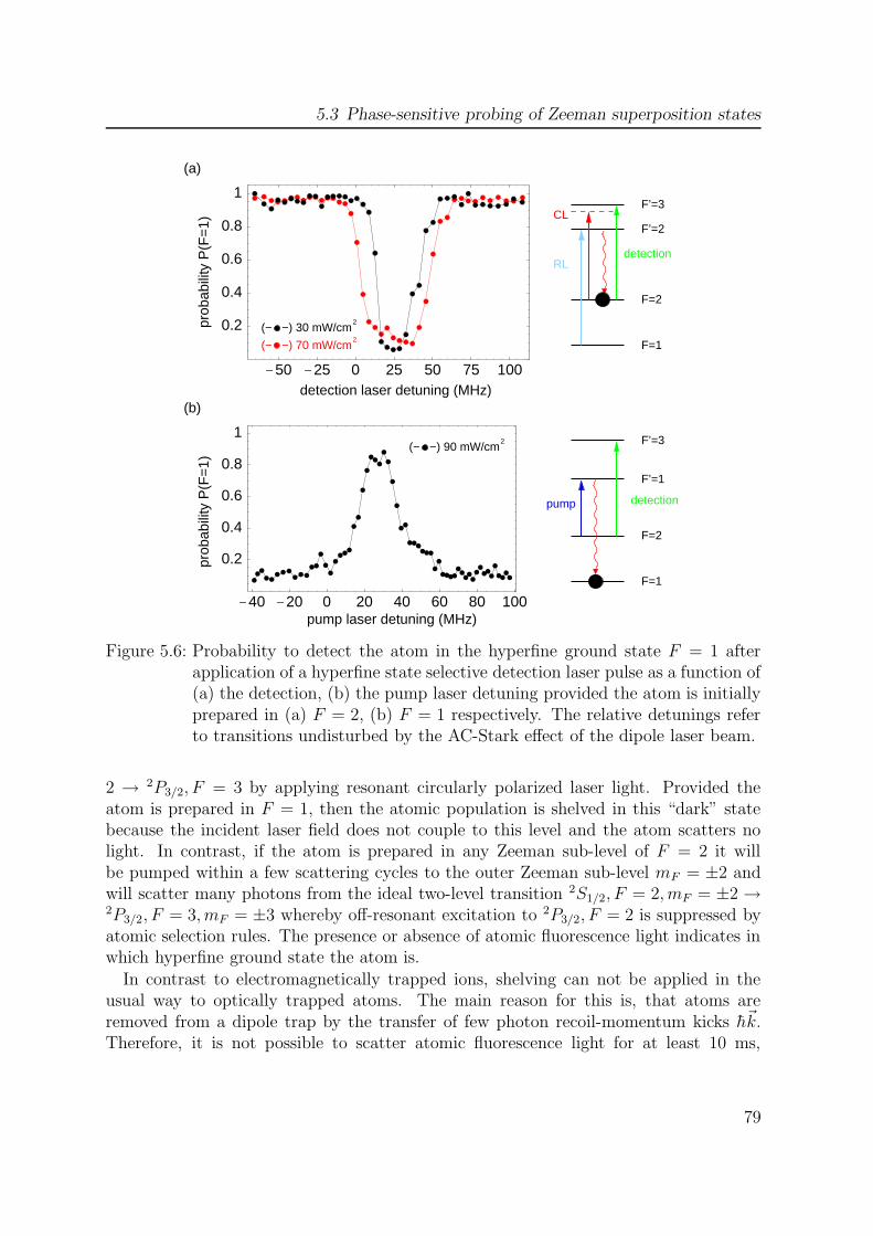
5.3 Phase-sensitive probing of Zeeman superposition states
-50 -25 0 25 50 75 100
0.2
0.4
0.6
0.8
1
-40 -20 0 20 40 60 80 100
0.2
0.4
0.6
0.8
1
F=1
F=2
F’=3
F’=1
F=1
F=2
F’=2
F’=3pr
obab
ility
P(F
=1)
prob
abili
ty P
(F=
1)
pump detection
detection
CL
RL
(− −) 30 mW/cm2
(− −) 90 mW/cm2
pump laser detuning (MHz)
(a)
(b)
(− −) 70 mW/cm2
detection laser detuning (MHz)
Figure 5.6: Probability to detect the atom in the hyperfine ground state F = 1 afterapplication of a hyperfine state selective detection laser pulse as a function of(a) the detection, (b) the pump laser detuning provided the atom is initiallyprepared in (a) F = 2, (b) F = 1 respectively. The relative detunings referto transitions undisturbed by the AC-Stark effect of the dipole laser beam.
2 → 2P3/2, F = 3 by applying resonant circularly polarized laser light. Provided theatom is prepared in F = 1, then the atomic population is shelved in this “dark” statebecause the incident laser field does not couple to this level and the atom scatters nolight. In contrast, if the atom is prepared in any Zeeman sub-level of F = 2 it willbe pumped within a few scattering cycles to the outer Zeeman sub-level mF = ±2 andwill scatter many photons from the ideal two-level transition 2S1/2, F = 2, mF = ±2 →2P3/2, F = 3, mF = ±3 whereby off-resonant excitation to 2P3/2, F = 2 is suppressed byatomic selection rules. The presence or absence of atomic fluorescence light indicates inwhich hyperfine ground state the atom is.
In contrast to electromagnetically trapped ions, shelving can not be applied in theusual way to optically trapped atoms. The main reason for this is, that atoms areremoved from a dipole trap by the transfer of few photon recoil-momentum kicks h~k.Therefore, it is not possible to scatter atomic fluorescence light for at least 10 ms,
79
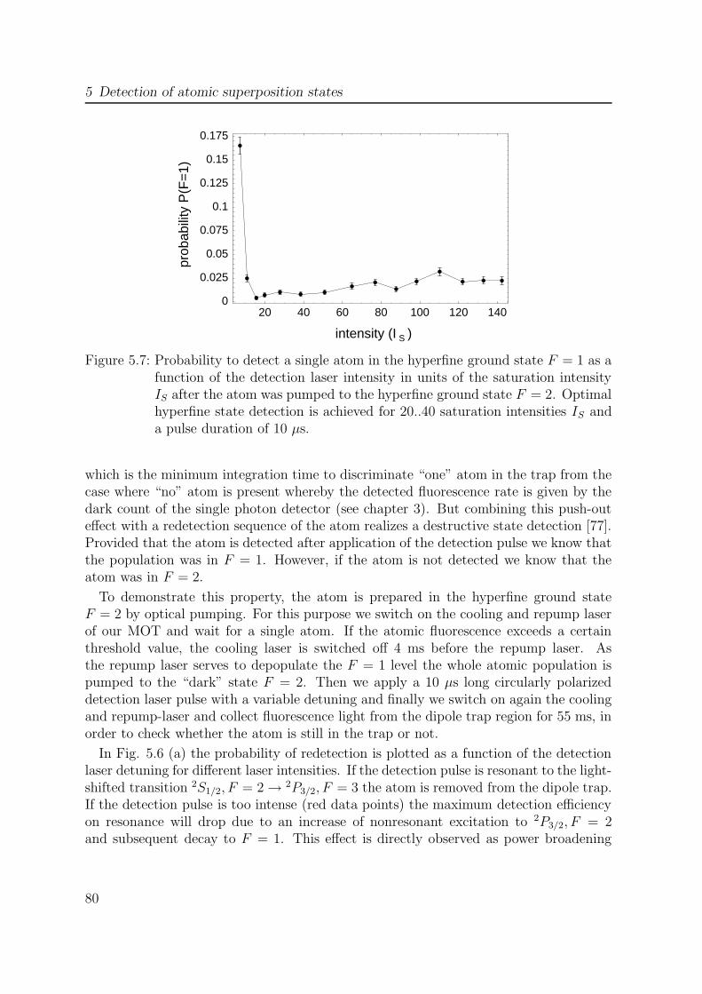
5 Detection of atomic superposition states
20 40 60 80 100 120 1400
0.025
0.05
0.075
0.1
0.125
0.15
0.175
Sintensity (I )
prob
abili
ty P
(F=
1)
Figure 5.7: Probability to detect a single atom in the hyperfine ground state F = 1 as afunction of the detection laser intensity in units of the saturation intensityIS after the atom was pumped to the hyperfine ground state F = 2. Optimalhyperfine state detection is achieved for 20..40 saturation intensities IS anda pulse duration of 10 µs.
which is the minimum integration time to discriminate “one” atom in the trap from thecase where “no” atom is present whereby the detected fluorescence rate is given by thedark count of the single photon detector (see chapter 3). But combining this push-outeffect with a redetection sequence of the atom realizes a destructive state detection [77].Provided that the atom is detected after application of the detection pulse we know thatthe population was in F = 1. However, if the atom is not detected we know that theatom was in F = 2.
To demonstrate this property, the atom is prepared in the hyperfine ground stateF = 2 by optical pumping. For this purpose we switch on the cooling and repump laserof our MOT and wait for a single atom. If the atomic fluorescence exceeds a certainthreshold value, the cooling laser is switched off 4 ms before the repump laser. Asthe repump laser serves to depopulate the F = 1 level the whole atomic population ispumped to the “dark” state F = 2. Then we apply a 10 µs long circularly polarizeddetection laser pulse with a variable detuning and finally we switch on again the coolingand repump-laser and collect fluorescence light from the dipole trap region for 55 ms, inorder to check whether the atom is still in the trap or not.
In Fig. 5.6 (a) the probability of redetection is plotted as a function of the detectionlaser detuning for different laser intensities. If the detection pulse is resonant to the light-shifted transition 2S1/2, F = 2 → 2P3/2, F = 3 the atom is removed from the dipole trap.If the detection pulse is too intense (red data points) the maximum detection efficiencyon resonance will drop due to an increase of nonresonant excitation to 2P3/2, F = 2and subsequent decay to F = 1. This effect is directly observed as power broadening
80

5.3 Phase-sensitive probing of Zeeman superposition states
of the line shape. In a second experiment (see Fig. 5.6 (b)) the atom is prepared inthe hyperfine ground state F = 1 by an additional pump laser pulse before applyingthe push-out and redetection sequence. When the pump laser is on resonance with thelight-shifted hyperfine transition 2S1/2, F = 2 → 2P3/2, F = 1 the redetection probabilityreaches its maximum because the atom is more efficiently pumped into the dark stateF = 1 . Out of resonance the excitation probability to 2P3/2, F = 1 decreases, such thatthe atomic population basically remains in F = 2 and the atom is kicked out of the trap.
P2
3/2
P2
3/2
S2
1/2
S2
1/2
25 50 75 100 125 150 1750
25
50
75
100
125
150
CL
RLCL
pump (1 1)
(b)
(a)
(c)
F=1
F=2
RL
detection
detection
pump (2 1)
F=1
F=2
F’=1F’=2
F’=3
F=1
F=2
F’=1F’=2
F’=3
state preparation state detection
< 5 s 48 µs 10 µs 60 ms
num
ber
of s
ampl
es
counts per 60 ms
Figure 5.8: (a) Histogramm of photon counts per 60 ms during redetection after appli-cation of a hyperfine state selective detection laser pulse. Atoms prepared inF = 1 (black line) survive the detection pulse, whereas atoms in F = 2 (blueline) are removed from the dipole trap. (b), (c) timing sequence and partiallevel scheme of Rubidium 87 for state detection in F = 1 and F = 2, respec-tively. (Experimental parameters: detection laser intensity = 40 saturationintensities IS).
81

5 Detection of atomic superposition states
In both measurements the duration and intensity of the pump and detection laserpulses were not optimized to achieve efficient state detection within the shortest periodof time. In a sequence of adjustment measurements we scanned systematically the power(see fig. 5.7) and duration of the push-out pulse and we find that single atoms preparedin F = 2 are removed from the dipole trap with a probability of 0.99± 0.01 (see fig. 5.8(a)), whereas atoms in F = 1 survive this pulse and are redetected in the dipole trapwith a probability of 0.95± 0.01. These numbers are not corrected by accidental loss ofthe atom during the redetection sequence due to collisions with “hot” atoms from thebackground gas (see 3.4.1) or with cold atoms from the surrounding optical molasses andthey also include incomplete preparation of the atom due to inefficient optical pumping.
Conclusion
The application of a detection laser pulse resonant to the light-shifted cycling transition2S1/2, F = 2, mF = 2 → 2P3/2, F = 3, mF = 3 and subsequent redetection of the atomin the dipole trap allows to discriminate the hyperfine ground states F = 1 and F = 2of Rubidium 87 with a minimum efficiency of 0.95. This value gives the upper boundof the maximum visibility achievable in the two-particle correlation measurements usedfor the verification of atom-photon entanglement.
5.3.3 Preparation of Zeeman superposition states
The key element for the detection of the atomic qubit in complementary measurementbases is the state-selective adiabatic population transfer from a coherent superposi-tion of Zeeman sublevels |mF = −1〉 and |mF = +1〉 of the hyperfine ground stateF = 1 to the hyperfine ground state F = 2. To verify this important property ofour STIRAP-scheme it is necessary to prepare in a first step a well defined superposi-tion 1√
2(|mF = −1〉 + eiφ|mF = +1〉) of the Zeeman sublevels mF = −1 and mF = +1.
This task can be realized by two different techniques. One the one hand one could usedirectly the projective polarization measurement of a spontaneously emitted photon,whereby the polarization state of the photon is initially entangled with the magneticquantum number mF = ±1. Because this task requires a rather complicated controlof many experimental parameters including the well defined preparation of the entan-gled state it seems much more simple to populate directly a coherent superposition1√2(|mF = −1〉 + eiφ|mF = +1〉) by optical pumping into a coherent dark state. How-
ever, also this technique has its difficulties, because coherent population trapping in theZeeman substructure of a given atomic state is extremely sensitive to residual magneticfields. The reason for this sensitivity is the time dependence of Zeeman dark-statesdue to Larmor precession. In order to populate a stable Zeeman dark state by opticalpumping it is therefore necessary to reduce the magnetic field below a threshold value.
Because the atom is stored in an optical dipole trap which is located inside a UHVvacuum chamber, it is not possible to measure the magnetic field exactly at the position
82

5.3 Phase-sensitive probing of Zeeman superposition states
∆ EB
F’=1
F=1 F=1
F’=1
−1 −1 +1
+10
0
(b)(a)
π
π
Figure 5.9: Zeeman-splitting of a hyperfine transition F = 1 → F ′ = 1. If the linearpump laser polarization is (a) perpendicular to the magnetic field, the darkstate 1√
2(|mF = −1〉−eiφ|mF = +1〉) is not stable due to Larmor-precession,
(b) parallel to the magnetic field, the dark state |mF = 0〉 is an energy eigen-state of the system and stable.
of the atom with usual Hall- or magnetic flux probes. A way to avoid this difficultiesis to use the atom itself as a probe. Here I will show, how the Zeeman-splitting of thehyperfine ground state 2S1/2, F = 1 allows to minimize the magnetic field and thereforeenables the population of coherent Zeeman-superposition states by optical pumping.
Time-dependence of Zeeman superposition states
Consider the simplified case of an atomic transition consisting of a single hyperfineground-state F = 1 and a single excited hyperfine state F ′ = 1. For laser light whoselinear polarization direction is orthogonal to the quantization axis z and parallel to y(φ = 0), the state
|S0〉 =1√2(|mF = −1〉 − |mF = +1〉) (5.15)
is dark.
Provided, the level-shift of the bare atomic states |F = 1, mF = −1〉 and |F = 1, mF = +1〉due to interaction with a magnetic field is small compared to the hyperfine-splitting, theZeeman-splitting ∆EB is given in first order perturbation theory by
hωL = ∆EB = µBgFmF |Bz|, (5.16)
where ωL is the Larmor frequency, µB denotes Bohrs magneton, gF the hyperfine-Lande-factor, mF the magnetic moment and |Bz| the absolute value of the magnetic field inz-direction. The time-evolution of the state |S0〉 is then given by
|S(t)〉 =1√2(|mF = −1〉 − e+2iωLt|mF = +1〉). (5.17)
83
5 Detection of atomic superposition states
After a characteristic time T = π/2ωL, the atom precessed into the orthogonal quan-tum state, which is a bright state for the incident linearly polarized laser field and theatom scatters photons until it is pumped again into the dark state |S0〉. The magnitudeof the magnetic field determines the time-evolution of the dark state and therefore therate of scattered photons.
Similar considerations are valid for a linearly polarized laser whose polarization direc-tion is parallel to the x-axis. In the case of π-polarized light - the linear polarizationdirection now is parallel to the magnetic field - the atom is pumped in the energyeigenstate |F = 1, mF = 0〉. However, this state is stable in time, independent of themagnitude of the magnetic field pointing along z. Provided the linear polarization di-rection of a pump laser field - resonant to the hyperfine transition F = 1 → F ′ = 1- is perpendicular to the magnetic field, the rate of scattered photons increases, as themagnitude of the magnetic field increases. For a “zero” field the rate is minimal. Thiseffect, similar to the Hanle-effect, is used in the present experiment to minimize themagnetic field for efficient preparation of atomic superposition states.
Magnetic field compensation
To minimize the magnetic field we shine on the optically trapped 87Rb atom a 1.8 mslinearly polarized dichromatic laser pulse resonant to the hyperfine transitions 2S1/2, F =1 → 2P3/2, F
′ = 1 and 2S1/2, F = 2 → 2P3/2, F′ = 1 and vary the magnetic field
orthogonal to the given linear polarization direction of the pump beams by adjustingthe current in the compensation coils. Then we redetect the atom in the dipole trap.If the magnetic field is minimal the atom scatters only few photons during the 1.8 msand therefore has the highest probability to survive. This procedure is performed for allthree componenents Bx, By and Bz of the magnetic field vector by rotating the linearpolarization of the pump beam and scanning the respective orthogonal magnetic fieldcomponent. From the measured experimental data in Fig. 5.10 and with the knowledgeof the geometry of the compensation coils we can determine an upper bound of theresidual magnetic field of 300 mGauss. This value is confirmed by the observation of aLarmor-precession frequency of 370 kHz [81] corresponding to a magnetic field of 132mGauss.
84

5.3 Phase-sensitive probing of Zeeman superposition states
0.2 0.4 0.6 0.8 1 1.2 1.4
0.2
0.4
0.6
0.8
1
1 1.2 1.4 1.6 1.8 2 2.2 2.4
0.2
0.4
0.6
0.8
1
0.25 0.5 0.75 1 1.25 1.5 1.75
0.2
0.4
0.6
0.8
1
prob
abili
ty P
(F=
1)pr
obab
ility
P(F
=1)
prob
abili
ty P
(F=
1)
lin.pol. || y
lin.pol. || z
lin.pol. || z
(a.u.)B z
(a.u.)B y
(a.u.)B x
(a)
(b)
(c)
Figure 5.10: Probability to detect the atom in the dipole trap after application of a 1.8ms pump pulse as a function of the magnetic compensation field in x-,y- andz-direction. If the respective magnetic field component is minimal, the atomis effectivly pumped into the stable Zeeman dark-state F = 1, mF = 0, andscatters no light. Therefore, the atom has a high survival probability.
85

5 Detection of atomic superposition states
P23/2
S21/2
F = 1
F = 2
F’ = 1F’ = 2
CL
Figure 5.11: Preparation of a Zeeman-superposition state 1√2(|1,−1〉 − |1,+1〉) via co-
herent population trapping (CPT). To avoid a dark state in F = 2 weadditionally apply the unpolarized cooling laser (CL) of our MOT.
State preparation
To prepare an atomic superposition state
|Sprep〉 =1√2(|1,−1〉 − |1,+1〉) (5.18)
via coherent population trapping (CPT) we apply a 5-µs linearly polarized (parallel toy) laser pulse resonant to the hyperfine transition 2S1/2, F = 1 → 2P3/2, F
′ = 1. Becausethis simple light field configuration pumps the atom also to a dark state of the hyperfineground level F = 2 we apply simultaneously two additional laser fields, depopulatingF = 2 (see Fig. 5.11).
5.3.4 Detection of Zeeman superposition states
Now, the prepared atomic superposition state |Sprep〉 can be analyzed by a state-selectiveStimulated-Raman-Adiabatic-Passage (STIRAP) technique. So far, the experimentalsetup as shown in chapter 3 was only slightly modified by pump beams which have beenderived from cooling and repump lasers of the MOT. But for the adiabatic populationtransfer additional lasers are necessarily operating at 795 nm. Before focussing on theexperimental results I will first give a short overview about the extended experimentalsetup.
Experimental setup
The STIRAP-pulses are generated by two independent laser diodes locked via Doppler-free saturation spectroscopy [77] to the hyperfine transitions 2S1/2, F = 1 → 2P1/2, F = 1and 2S1/2, F = 2 → 2P1/2, F = 1 of the D1-line in Rubidium 87. The shape of eachpulse (amplitude and duration) is adjusted by an AOM in double-pass configuration
86

5.3 Phase-sensitive probing of Zeeman superposition states
ST ST
λ/2
spectroscopy
1 2
AOM 1 AOM 2
to AOM 3
λ/4 λ/4
PBS
Figure 5.12: Experimentel setup of the STIRAP-lasers. (ST1 ... STIRAP-laser 1, ST1 ...STIRAP-laser 2, PBS ... polarizing beam splitter, AOM ... acousto-opticalmodulator, λ/2 ... half wave plate, λ/4 ... quarter wave plate)
down to a minimum pulse length of approximatly 15 ns. The delay of the Stokes pulsewith respect to the pump pulse is controlled by a tuneable electric delay line and aprogrammable pattern generator [124], which allows to switch on and off the AOMswith a time resolution of 20 ns. The pump and Stokes beams are overlapped on apolarizing beam-splitter (PBS) and coupled into a single mode optical fiber. Becausethe STIRAP-pulses have to be applied to the atom in the observation direction of atomicfluorescence light, a good on/off-switching ratio of the AOMs is necessary to eliminateunwanted background light from the STIRAP-beams. An overall optical isolation ofapproximately 120 dB is realized by an additional acousto-optical modulator AOM3
switching both pulses after overlapping.
To connect the preparation part of the STIRAP pulses (see Fig. 5.12) with the trapsetup (see Fig. 5.13) the STIRAP beams are coupled again into a single mode opticalfiber. At the exit port of the fiber a rotable half-wave plate (λ/2) is used to adjustthe linear polarization angle α of the STIRAP pulses Ω1 and Ω2. In addition a tiltedbirefringent crystall (C) compensates for relative phase shifts between s- and p- polarizedcomponents that occur at the reflection on dielectric mirrors. Finally the STIRAP-pulsesare focussed with an objective onto the atom to a waist of 5..10 µm.
For the preparation and analysis of atomic superposition states additional pump anddetection beams resonant to specific hyperfine transitions within the D2-line of Rubidium87 are necessary. Therefore different beams are extracted from the cooling and repumplasers and switched independently by AOMs in double-pass configuration. Then eachbeam is coupled into a single-mode optical fiber and focussed onto the atom.
87

5 Detection of atomic superposition states
PD
FC
C
MOT beams
MOT beams
x
z
y
z
(a) (b)
from STIRAP laser @ 795 nm
λ/2λ/2
DM
detection
pump
Figure 5.13: Schematic view of the experimental setup to investigate a coherent superpo-sition of the Zeeman states |F = 1, mF = −1〉 and |F = 1, mF = +1〉. (a)horizontal view; (b) upright view.
Experimental process
To verify the selective detection of Zeeman-superposition states via STIRAP, we firstload a single 87Rb atom into the dipole trap. Then a 5-µs optical laser pulse (seepreceding section) pumps the atomic population into the dark superposition state
|Sprep〉 =1√2(|1,−1〉 − |1,+1〉) (5.19)
of the 2S1/2, F = 1 ground level. To analyze this state we apply immediatly after thepreparation pulse a 70 ns STIRAP-pulse, transferring a superposition state
|Strans〉 =1√2(|1,−1〉 − e2iα|1,+1〉) (5.20)
adiabatically to the hyperfine ground state F = 2. Due to destructive interference of theexcitation amplitudes the orthogonal quantum state |Sdark〉 = 1√
2(|1,−1〉 + e2iα|1,+1〉)
does not couple to the STIRAP laser field Ω1 and remains in F = 1. The relative phaseof these states can be controlled by the linear polarisation angle α of the STIRAP laserΩ1 with respect to the x-axis. After the transfer we apply a hyperfine state selective40 µs push-out laser pulse to discriminate the hyperfine ground states. Finally the
88
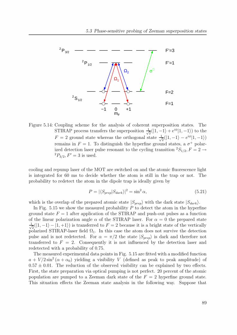
5.3 Phase-sensitive probing of Zeeman superposition states
σ+
Ω1
Ω2
P23/2
P21/2
S21/2
0 +1−1F=1
F=2
mF
F’=1
F’=3
Figure 5.14: Coupling scheme for the analysis of coherent superposition states. TheSTIRAP process transfers the superposition 1√
2(|1,−1〉+ eiφ|1,−1〉) to the
F = 2 ground state whereas the orthogonal state 1√2(|1,−1〉 − eiφ|1,−1〉)
remains in F = 1. To distinguish the hyperfine ground states, a σ+ polar-ized detection laser pulse resonant to the cycling transition 2S1/2, F = 2 →2P3/2, F
′ = 3 is used.
cooling and repump laser of the MOT are switched on and the atomic fluorescence lightis integrated for 60 ms to decide whether the atom is still in the trap or not. Theprobability to redetect the atom in the dipole trap is ideally given by
P = |〈Sprep|Sdark〉|2 = sin2 α, (5.21)
which is the overlap of the prepared atomic state |Sprep〉 with the dark state |Sdark〉.In Fig. 5.15 we show the measured probability P to detect the atom in the hyperfine
ground state F = 1 after application of the STIRAP and push-out pulses as a functionof the linear polarization angle α of the STIRAP laser. For α = 0 the prepared state1√2(|1,−1〉 − |1,+1〉) is transferred to F = 2 because it is a bright state of the vertically
polarized STIRAP-laser field Ω1. In this case the atom does not survive the detectionpulse and is not redetected. For α = π/2 the state |Sprep〉 is dark and therefore nottransferred to F = 2. Consequently it is not influenced by the detection laser andredetected with a probability of 0.75.
The measured experimental data points in Fig. 5.15 are fitted with a modified functiona + V/2 sin2 (α + α0) yielding a visibility V (defined as peak to peak amplitude) of0.57 ± 0.01. The reduction of the observed visibility can be explained by two effects.First, the state preparation via optical pumping is not perfect. 20 percent of the atomicpopulation are pumped to a Zeeman dark state of the F = 2 hyperfine ground state.This situation effects the Zeeman state analysis in the following way. Suppose that
89

5 Detection of atomic superposition states
20 percent of the atomic population are in F = 2 and 80 percent are ideally in theprepared dark state 1√
2(|1,−1〉 − |1,+1〉). Then, if the polarization of the STIRAP
laser is chosen such that it couples maximally to the prepared superposition in F = 1and maximally to the population in F = 2, the fraction in F = 1 will be transferredto F = 2, whereas population initially in F = 2 is partially transferred to F = 1.Suppose the STIRAP laser does not couple to the superposition in F = 1 becausethe prepared Zeeman superposition state is a dark state with respect to the chosenpolarisation, then population in F = 2 will be partially transferred to F = 1. To getan estimation about the impact of this process on the measured data we numericallysolved a master equation of the STIRAP-process on the basis of a simplified three-levelmodel including spontaneous emission from the intermediate level. We get the resultthat after the STIRAP-pulse maximally 84 percent of the atomic population will be inF = 1 provided the STIRAP polarization is chosen such that the STIRAP does notcouple to the prepared Zeeman state in F = 1, whereas if the STIRAP couples initiallyto population in F = 1 and F = 2, after the pulse 5 percent will remain in F = 1. Onthe basis of this estimation we calculate a corrected visibility of 0.71 ± 0.01.
A second important source of errors is the imperfect state transfer via the STIRAPpulses. For further optimization of the process, it is useful to decouple the inefficientstate preparation from the state detection. After all, the preparation of a “clean” initialatomic state can be best realized by the polarization measurement of a spontaneouslyemitted photon, provided the photon was initially entangled with the Zeeman statemF = ±1 of the atom.
5.4 Conclusion and discussion
We have set up a laser system which allows to read out a Zeeman superposition stateof a single atom. Depending on the polarisation of the STIRAP pulses a superposition1√2(|F = 1, mF = −1〉 + eiφ|F = 1, mF = +1〉) of the 2S1/2, F = 1, mF = ±1 hyperfine
ground state is adiabatically transferred to the F = 2 state. Due to destructive interfer-ence of the excitation amplitudes the orthogonal quantum state 1√
2(|F = 1, mF = −1〉−
eiφ|F = 1, mF = +1〉) does not couple to the STIRAP pulse and remains in F = 1. Todiscriminate these states we apply a detection laser pulse resonant to the cycling transi-tion 2S1/2, F = 2 → 2S1/2, F
′ = 3. Provided the atom is in F = 2 it scatters photons fromthis laser beam, and with each scattering event the atom acquires an additional photonmomentum h~k. After approximately 40 to 50 scattering events the atom is pushed outof the dipole trap. Finally, to read out the atomic state the cooling and repump beamsof the MOT are switched on and the atomic fluorescence light is integrated for 60 ms todecide if the atom is still in the trap or not.
90
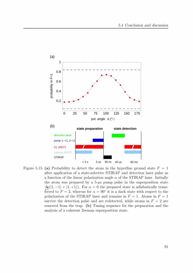
5.4 Conclusion and discussion
STIRAP
0 25 50 75 100 125 150 175
0.2
0.4
0.6
0.8
1
α (°)pol. angle
(a)
(b)
60 ms40 µs
prob
abili
ty in
F=
1
5 µs< 2 s
CL (MOT)
pump 1−>1, 2−>1
detection laser
repump (MOT)
60 ns
state preparation state detection
Figure 5.15: (a) Probability to detect the atom in the hyperfine ground state F = 1after application of a state-selective STIRAP and detection laser pulse asa function of the linear polarization angle α of the STIRAP laser. Initiallythe atom was prepared by a 5-µs pump pulse in the superposition state1√2(|1,−1〉 + |1,+1〉). For α = 0 the prepared state is adiabatically trans-
ferred to F = 2, whereas for α = 90 it is a dark state with respect to thepolarization of the STIRAP laser and remains in F = 1. Atoms in F = 1survive the detection pulse and are redetected, while atoms in F = 2 areremoved from the trap. (b) Timing sequence for the preparation and theanalysis of a coherent Zeeman superposition state.
91
6 Observation of atom-photon
entanglement
6.1 Introduction
Atom-photon entanglement has been implicit in many previous experimental systems,from early measurements of Bell’s inequality violations in atomic cascade systems [4, 6]to fluorescence studies in trapped atomic ions [28, 29] and atomic beam experiments [30].However, it has not been directly observed until quite recently [35], as the individualatoms and photons have not been under sufficient control.
In our experiment a single photon is spontaneously emitted from a single opticallytrapped 87Rb atom, which is initially excited to a state which has multiple decay chan-nels. Along a certain emission direction two decay channels are selected and the photonpolarization is maximally entangled with two particular Zeeman sublevels of the hyper-fine ground states of the atom.
To verify entanglement of the generated atom-photon state one has to disprove thepossibility that the two-particle quantum system can be a statistical mixture of seperablestates. This task is closly connected to a violation of Bell’s inequality and requiresscorrelated local state measurements of the atom and the photon in complementary bases.
In this chapter I will report in detail on the generation and analysis of atom-photonentanglement. The experimental process is described and first experimental results arediscussed confirming spin-entanglement between the atom and the photon.
6.2 Experimental process
First, we load a single 87Rb atom from a magneto-optical trap - operated in a pulsedmode - into the optical dipole trap. Then a 5.5-µs linearly polarized optical pulse pumpsthe atom into the 2S1/2, |1, 0〉 dark state (for details see preceding chapter), from wherethe atom is excited by a 30-ns π-polarized optical π-pulse to the 2P3/2, |0, 0〉 state. Here|F,mF 〉 denotes the internal atomic quantum numbers of the total angular momentumand its projection along the quantization axis z.
In the following spontaneous emission the atom decays either to the |1,−1〉 groundstate while emitting a photon in the polarization state |σ+〉, or to the |1, 0〉 state whileemitting a |π〉-polarized photon or it decays to the |1,+1〉 ground state and emits a|σ−〉-polarized photon. Because the residual magnetic field is smaller than 100 mGauss,
92

6.2 Experimental process
1,00,0
S 1/2
2
P 3/2
2
S 1/2
2
P 1/2
2
σ+ σ−
σ+
P , F=33/2
2
1,−1 1,+11,−1 1,+11,0
Ω1
Ω1
Ω2
Ω2
σ+
780 nm
(a)
795 nm
6.8 GHz
(b)
F=1
F=2
F=1
F=2
initial state preparation
5.5 µs
atomic state detection
30 ns
6 µs
55 ms
70 ns
excitation
optical pumping
−
photon detection
STIRAP
redetection (MOT)
70 ns
detection
STI
Figure 6.1: The experimental process (time not to scale). (a) The atom is initializedto the |1, 0〉 hyperfine ground state by optical pumping (not shown) andexcited by a 30-ns π-polarized π-pulse to the |0, 0〉 excited state. In thefollowing spontaneous decay the polarization state of the photon is entan-gled with magnetic hyperfine state of the atom. (b) After the polarizationmeasurement of the photon the internal state of the atom is measured by a70-ns STIRAP and a 6-µs detection pulse, before atomic fluorescence lightis accumulated for 55 ms.
the Zeeman-splitting of these states is two orders of magnitude smaller than the naturallinewidth of the transition. Therefore these decay channels are spectrally indistiguishableand a coherent superposition of separable atom-photon states is formed, entangling themagnetic quantum number mF of the atom with the polarization state of the emittedphoton. Along the observation direction, defined by the aperture of the microscopeobjective, π-polarized photons are not emitted. Thus, the resulting atom-photon stateis maximally entangled:
|Ψ+〉 =1√2(|1,−1〉|σ+〉 + |1,+1〉|σ−〉). (6.1)
93

6 Observation of atom-photon entanglement
Figure 6.2: Simplified setup of the experimental apparatus. The π-polarized excitationbeam propagates perpendicular to the quantization axis z defined by theoptical axis of the detection optics. The scattered photons are collectedby a microscope objective, coupled to a single mode optical fiber and di-rected to a polarizing beam splitter (PBS). Two single photon detectorsAPD1 and APD2 register the H- and V-polarized photons, respectively. Theλ/2-waveplate is used to rotate the photon polarization for photonic qubitmeasurements in different bases. The atomic state is analysed by a STIRAP-pulse driving coherent two-photon transitions between the hyperfine levelsof the atomic ground state. The atomic measurement basis is defined by theangle α of the linearly polarized STIRAP laser field Ω1 with respect to they-axis.
To investigate the nonclassical correlation properties of this state, the single photonfrom the spontaneous decay is collected with a microscope objective (see Fig. 6.2) andcoupled into a single-mode optical fiber guiding it to a polarization analyzer consistingof a rotable λ/2-halfwave plate, a polarizing beam splitter (PBS) and two avalanchephoto-diodes APD1 and APD2 for single photon detection. Triggered by the detectionof a photon, the internal quantum state of the atom is analyzed by a state-selectiveStimulated-Raman-Adiabatic-Passage (STIRAP) technique transferring the superposi-tion 1√
2(|1,−1〉 + e2iα|1,+1〉) to the hyperfine ground state F=2 (see chapter 5). Due
to destructive interference of the excitation amplitudes the orthogonal quantum state
94

6.2 Experimental process
1√2(|1,−1〉 − e2iα|1,+1〉) does not couple to the STIRAP laser field Ω1 (see Fig. 6.1(a))
and remains in F = 1. Here the relative phase 2α is defined by the linear polar-ization angle α of the STIRAP laser Ω1 with respect to the y-axis. The phase set-tings α = 0, π/2 and α = π/4, 3π/4 define two sets of complementary basis-states 1√
2(|1,−1〉 + |1,+1〉), 1√
2(|1,−1〉 − |1,+1〉) and 1√
2(|1,−1〉 + i|1,+1〉), 1√
2(|1,−1〉 −
i|1,+1〉), which allow to measure the atomic qubit in the σx- and σy-basis, whereby|1,±1〉 are eigenstates of σz.
1000 2000 3000 4000 5000 6000
20406080
100120140
5625 5650 5675 5700 5725 5750 5775
10
20
30
40
50
spontaneous emission
(b)
(a)
τ = 28 ns
time (ns)
STIRAP straylight
time (ns)
initial state preparationnum
ber
num
ber
Figure 6.3: Number of scattered photons as a function of time during (a) preparationof the initial state via optical pumping into the dark state 2S1/2, |1, 0〉 (in-tegration time bin ∆t = 8ns), (b) excitation to 2P3/2, |0, 0〉 and subsequentspontaneous decay to 2S1/2, |1,±1〉 (integration time bin ∆t = 2ns).
95
6 Observation of atom-photon entanglement
After the state-selective population transfer the atom is in a superposition of thehyperfine ground states F = 1 and F = 2. To discriminate these states we apply a 6-µsdetection laser pulse resonant to the cycling transition 52S1/2, F = 2 → 52P3/2, F = 3.If the atom is in the hyperfine ground state F = 2, it is removed from the dipole trapdue to photon recoil heating. If the atom was in state F = 1, fluorescence is observedafter the cooling and repump lasers of the MOT are switched on. Counts are integratedfor 55 ms to decide whether the atom is still in the trap or not.
In Fig. 6.3 the number of scattered photons during the preparation of the initialstate 2P3/2, |0, 0〉 is shown as a function of time. When the pump pulse is switched on,the number of scattered photons decreases after few 100 ns as the atomic populationis pumped to the Zeeman dark state 2S1/2, |1, 0〉. The intensity of the following 30-ns optical π-pulse is chosen such, that at the end of the pulse the maximum atomicpopulation is in the 2P3/2, |0, 0〉 state. In the following spontaneous decay - indicated bythe red data trace in Fig. 6.3(b) - the number of scattered photons drops exponentiallywith a measured time constant of 28 ns. To correlate the atomic state detection with theinternal state of a spontaneously emitted photon we restrict the detection of photons toa well defined time window of 70 ns following the optical excitation pulse (see Fig. 6.1).
The generation of entangled atom-photon pairs is probabilistic because a sponta-neously emitted photon is detected with a probability of η = 5×10⁻⁴. This means, thatthe atom has to be excited approximately 2000 times until a photon is detected. Toachieve the best rate of detected atom-photon pairs, the excitation cycle - consisting ofoptical pumping to 52S1/2, |1, 0〉 and following excitation to 52P3/2, |0, 0〉 - is repeated aslong until a photon is detected. Once a photon is detected the atom is measured withalmost perfect efficiency, limited only by loss from the dipole trap during the fluorescencedetection.
6.3 Experimental results
To verify atom-photon entanglement we measure the conditional probability of detectingthe atomic qubit in the complementary bases σx and σy as a function of the polarizationstate of the detected photon.
In Fig. 6.4(a) the polarisation of the STIRAP-lasers is set to α = 0 defining theσx measurement basis for the atom and the polarization of the photon is rotated onthe Poincare-sphere by a variable angle 2β. We observe strong correlations betweenthe polarization state of the detected photon and the internal quantum state of theatom. As expected, if the photon is detected in the polarization state 1√
2(|σ+〉 + |σ−〉)
(detection in APD1) the atom is projected to the corresponding superposition state1√2(|1,−1〉+|1,−1〉). This atomic state is a “dark” state for the chosen linear polarization
of the STIRAP laser field Ω1. Hence the atomic population will remain in F = 1 afterthe STIRAP-pulse. If the photonic qubit is rotated by a phase of φ = π before statereduction the single photon detectors exchange their role and a detection at APD1
96

6.4 Conclusion and discussion
projects the atom to 1√2(|1,−1〉 − |1,−1〉). Now, this atomic state can be transferred
to the hyperfine ground state F = 2, i.e. P (F = 1) goes to a minimum. From a fitof the measured correlations we obtain a visibility (defined as peak to peak amplitude)of 0.81 ± 0.04. To verify entanglement this measurement has to be repeated for anatomic basis conjugate to the first one. Thus the atomic qubit was analyzed in thecomplementary σy basis (see Fig. 6.4(b)). Therefore the STIRAP polarization angle αis set to π/4. Again, strong correlations are observed with a visibility of 0.70 ± 0.04.But now the measured atom-photon correlations are shifted by β = π/4, as we expectfrom an entangled state.
To quantify the amount of entanglement we determine the entanglement fidelity F =〈Ψ+|ρ|Ψ+〉, which is defined as the overlap of the measured state - characterized bythe density matrix ρ - with the maximally entangled state |Ψ+〉 we expect to generate.Because the atomic state detection is imperfect, we model these errors by a quantumchannel which is subjected to white noise. Therefore, the density matrix of the detectedstate can be expressed as ρ = V |Ψ+〉〈Ψ+| + 1−V
41, where V is the mean visibility of
the observed correlations in the two complementary bases. From this we derive anentanglement fidelity of 0.82 ± 0.04.
6.4 Conclusion and discussion
In the current experiment we excite a single optically trapped 87Rb atom by a shortoptical pulse to a state which has multiple decay channels and detect the subsequentspontaneously emitted single photon. Along a certain emission direction - defined bythe optical axis of the detection optics - two decay channels are selected and the photonpolarization is maximally entangled with two particular Zeeman sublevels of the hy-perfine ground states of the atom. The entanglement is directly verified by appropriatepolarization analysis of the photon and Zeeman state detection of the trapped atom. Weobserve strong atom-photon correlations in complementary measurement bases yieldingan entanglement fildelity of 0.82 ± 0.04.
97

6 Observation of atom-photon entanglement
-40 -20 0 20 40
0.2
0.4
0.6
0.8
1
-40 -20 0 20 40
0.2
0.4
0.6
0.8
1pr
obab
ility
P(F
=1)
prob
abili
ty P
(F=
1)
photonic analysis angle β/2 (°)
photonic analysis angle β/2 (°)
APD2
APD1
APD2
APD1
(b)
(a)
Figure 6.4: Probability of detecting the atom in the ground state F = 1 (after theSTIRAP pulse) conditioned on the detection of the photon in detector APD1
(red data points) or detector APD2 (blue data points) as the phase φ = 2βof the photonic rotation is varied. The atomic qubit is projected (a) tothe states 1/
√2(|1,−1〉± |1,+1〉), (b) to the states 1/
√2(|1,−1〉± i|1,+1〉)
corresponding to a spin measurement in σx and σy, respectively, whereas thephotonic qubit is projected onto the states 1√
2(|σ+〉 ± eiφ|σ−〉).
98
7 Conclusion and Outlook
The goal of this thesis was the experimental generation and analysis of entanglementbetween the spin state of a single neutral 87Rb atom and the polarization state of a singlespontaneously emitted photon suitable for long-distance transport in optical fibers andair. This task required in a first step the efficient detection and manipulation of a single87Rb atom. For this purpose a far-off-resonance optical dipole trap was set up. Becauseof the small trap volume and due to light-induced two-body collisions, which are presentduring the loading stage within the light fields of a magneto-optical trap, only singleatoms are captured. This blockade effect was confirmed by the observation of photonantibunching in the detected fluorescence light. To generate the entangled atom-photonstate the atom is excited to a state which has two decay channels. Due to conservationof angular momentum in the following spontaneous emission the polarization state ofthe photon is maximally entangled with two particular Zeeman sub-levels of the atomicground state. To detect entanglement of this atom-photon state we performed correlatedlocal measurements of the polarization state of the photon and the internal quantumstate of the atom. The atomic spin state was analyzed by means of a Stimulated-Raman-Adiabatic-Passage (STIRAP) process, where the polarization of the analyzing laser lightdefined the atomic measurement basis. Strong nonclassical atom-photon correlations incomplementary measurement bases were observed yielding an entanglement fidelity of0.82 ± 0.04.
The realization of entanglement between a single optically trapped 87Rb atom and aspontaneously emitted single photon described in this work marks a first successful steptowards the remote state preparation of a single atom over large distances and a firstloophole-free test of Bell’s inequality [13, 14].
Remote state preparation of a single atom
A first step towards entanglement swapping or the closely related quantum teleporta-tion is the so-called remote state preparation [125, 126]. In this protocoll generic, stateindependent unitary transformations U on the atom are sufficient to prepare it in thearbitrary quantum state |ΨB〉 = cosα|↑〉 − sinαeiβ|↓〉. This process works as follows:Suppose a single atom is entangled with a single photon. Then the photon propagatesto Alice who performs a unitary operation U(α, β) with two free parameters α, β in anextended four-dimensional Hilbert space, before she projects the photon onto a general-ized Bell-basis [127]. Depending on her measurement result, Bob now has to perform aunitary spin rotation U in order to prepare the required quantum state of the atom.
99

7 Conclusion and Outlook
ΨAB
ΨB
entangled state
A B
Alice
classical information
Bob
U(α,β)
M
U
Figure 7.1: Principle of Remote State Preparation.
This scheme generalizes to teleportation, if one introduces yet another photon, al-lowing a direct transfer of a photonic qubit to an atom which can be used for robustlong-term storage of quantum information. To reconvert the stored information onto asingle photon one can reexcite the atom on a so-called V-type transition [128]. Further-more, if one puts the atom into a high Q cavity, it is possible to force the atom to emitthe photon into one selected spatial mode. These properties fulfill all requirements forefficient quantum networking. But teleportation or entanglement swapping is the keyfor a loophole free Bell experiment.
Loophole-free test of Bell’s inequality
For a loophole-free test of Bell’s inequality one needs two entangled quantum systemswhich can be detected with high efficiency and which are separated far enough that localobservations of each system are space-like separated. This task can be accomplishedby two entangled atoms. First, atoms have the important property that they can bedetected with almost perfect efficiency. Second, entanglement between two distant atomscan be generated in a robust way by an entanglement swapping [15] process between twoindependently created entangled atom-photon pairs [13, 14]. Suppose one starts withtwo atoms in two distant traps, where in each trap only one atom is stored. Then eachatom is entangled with one spontaneously emitted photon. The independently generatedphotons then propagate to an intermediate location where a partial Bell-state analysisis performed, projecting the atoms onto an entangled state.
In the present experiment verifying atom-photon entanglement the atomic state de-tection is performed with an efficiency of one because every state measurement givesa result. Hence, the measured entanglement fidelity already includes all experimentalerrors of the atomic state detection and no additional fair-sampling assumption has tobe made for a Bell test with entangled atoms. To close at the same time the localityloophole, the atoms have to be space-like separated with respect to the duration of the
100
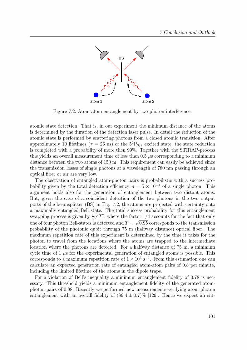
7 Conclusion and Outlook
BS
atom 1 atom 2
Figure 7.2: Atom-atom entanglement by two-photon interference.
atomic state detection. That is, in our experiment the minimum distance of the atomsis determined by the duration of the detection laser pulse. In detail the reduction of theatomic state is performed by scattering photons from a closed atomic transition. Afterapproximately 10 lifetimes (τ = 26 ns) of the 52P3/2 excited state, the state reductionis completed with a probability of more then 99%. Together with the STIRAP-processthis yields an overall measurement time of less than 0.5 µs corresponding to a minimumdistance between the two atoms of 150 m. This requirement can easily be achieved sincethe transmission losses of single photons at a wavelength of 780 nm passing through anoptical fiber or air are very low.
The observation of entangled atom-photon pairs is probabilistic with a success pro-bability given by the total detection efficiency η = 5 × 10⁻⁴ of a single photon. Thisargument holds also for the generation of entanglement between two distant atoms.But, given the case of a coincident detection of the two photons in the two outputports of the beamsplitter (BS) in Fig. 7.2, the atoms are projected with certainty ontoa maximally entangled Bell state. The total success probability for this entanglementswapping process is given by 1
4η2T 2, where the factor 1/4 accounts for the fact that only
one of four photon Bell-states is detected and T =√
0.95 corresponds to the transmissionprobability of the photonic qubit through 75 m (halfway distance) optical fiber. Themaximum repetition rate of this experiment is determined by the time it takes for thephoton to travel from the locations where the atoms are trapped to the intermediatelocation where the photons are detected. For a halfway distance of 75 m, a minimumcycle time of 1 µs for the experimental generation of entangled atoms is possible. Thiscorresponds to a maximum repetition rate of 1× 10⁶ s−1. From this estimation one cancalculate an expected generation rate of entangled atom-atom pairs of 0.8 per minute,including the limited lifetime of the atoms in the dipole traps.
For a violation of Bell’s inequality a minimum entanglement fidelity of 0.78 is nec-essary. This threshold yields a minimum entanglement fidelity of the generated atom-photon pairs of 0.88. Recently we performed new measurements verifying atom-photonentanglement with an overall fidelity of (89.4 ± 0.7)% [129]. Hence we expect an ent-
101

7 Conclusion and Outlook
anglement fidelity of 80 % for the entangled atom-atom state. The loophole-free violationof a CHSH-type Bell’s inequality [40] by three standard deviations would require approx-imately 7000 atom pairs. On the basis of the above estimations a total measurementtime of 12 days should be feasible, starting with the performance of the setup developedin this work.
102

A Appendix
Table A.1: Physical properties of 87Rb [61].
Atomic Number Z 37Total Nucleons Z +N 87Relative Natural Abundance η 27.83(2) %Nuclear Spin I 3/2Atomic Mass m 86.9092 uVacuum Wavelength D1-Transition λD1 794.979 nmVacuum Wavelength D2-Transition λD2 780.246 nmLifetime 5 2P1/2 27.70 nsLifetime 5 2P3/2 26.24 nsNatural Line Width D1-Transition ΓD1 2π × 5.746(8) MHzNatural Line Width D2-Transition ΓD2 2π × 6.065(9) MHzGround State Hyperfine Splitting νHFS 6834.68 MHzRecoil Velocity D2-Transition vr 5.8845 mm/sRecoil Temperature D2-Transition Tr 361.95 nKDoppler Temperature D2-Transition TD 146 µKDipole Matrix Element D2-Transition 〈J ||er||J ′〉 3.584(4) × 10−29 C mSaturation Intensity52S1/2, F = 2, mF = ±2 → IS 1.67 mW/cm2
52P3/2, F = 3, mF = ±3 Transition
103
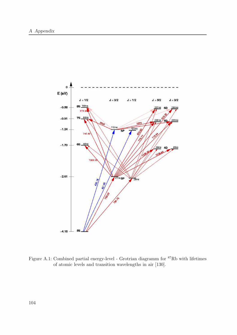
A Appendix
Figure A.1: Combined partial energy-level - Grotrian diagramm for 87Rb with lifetimesof atomic levels and transition wavelengths in air [130].
104

A Appendix
5P3/2
5P1/2
5S1/2
mF
F=3
F=2
F=1F=0
F=2
F=1
F=2
F=1
D1
@ 7
95 n
m
−3 −2 −1 0 +2+1 +3
D2
@ 7
80 n
m
267 MHz
157 MHz
72 MHz
813 MHz
6835 MHz
Figure A.2: Level scheme of 87Rb with nuclear spin I = 3/2.
105

Bibliography
[1] E. Schrodinger. Die gegenwartige Situtation in der Quantenmechanik. Naturwis-senschaften, 23:807–812, 823–828, 844–849, 1935.
[2] A. Einstein, B. Podolsky, and N. Rosen. Can quantum-mechanical description ofreality be considered complete ? Phys. Rev., 47:777–780, 1935.
[3] J. S. Bell. On the Einstein-Podolsky-Rosen Paradox. Physics, 1:195–200, 1964.
[4] S. J. Freedman and J. F. Clauser. Experimental test of Local Hidden-VariableTheories. Phys. Rev. Lett., 28:938, 1972.
[5] A. Aspect, P. Grangier, and G. Roger. Experimental Test of Realistic Local The-ories via Bell’s theorem. Phys. Rev. Lett., 47:460, 1981.
[6] A. Aspect, P. Grangier, and G. Roger. Experimental Realization of Einstein-Podolsky-Rosen-Bohm Gedankenexperiment. Phys. Rev. Lett., 49:91, 1982.
[7] G. Weihs, T. Jennewein, C. Simon, H. Weinfurter, and A. Zeilinger. Violationof Bell’s Inequality under Strict Einstein Locality Conditions. Phys. Rev. Lett.,81:5039, 1998.
[8] M. A. Rowe, D. Kielpinsky, V. Meyer, C. A. Sacket, W. M. Itano, C. Monroe,and D. J. Wineland. Experimental violation of a Bell’s inequality with efficientdetection. Nature, 409:791, 2001.
[9] J. S. Bell. Speakable and Unspeakable in Quantum Mechanics. Cambridge Univer-sity Press, Cambridge, 1988.
[10] E. Santos. Critical analysis of the empirical tests of local hidden-variable theories.Phys. Rev. A, 46:3646, 1992.
[11] P. Pearle. Hidden variable example based upon data rejection. Phys. Rev. D,2:1418, 1970.
[12] E. Santos. Constraints for the violation of the Bell inequality in Einstein-Podolsky-Rosen-Bohm experiments. Phys. Lett. A, 200:1, 1995.
106

Bibliography
[13] K. Saucke. Optische Dipolfalle fur Einzelatome. Master’s thesis, Ludwig-Maximilians-Universitat Munchen, 2002.
[14] C. Simon and T. M. Irvine. Robust Long-Distance Entanglement and a Loophole-Free Test with Ions and Photons. Phys. Rev. Lett., 91:110405, 2003.
[15] M. Zukowski, A. Zeilinger, M. A. Horne, and A. K. Ekert. “Event-ready-detectors”Bell experiment via entanglement swapping. Phys. Rev. Lett., 71:4287, 1993.
[16] D. Bouwmeester, A. Ekert, and A. Zeilinger. The Physics of Quantum Information.Springer-Verlag, Berlin, Heidelberg, 2000.
[17] I. Chuang and M. Nielsen. Quantum Computation and Quantum Information.Cambridge University Press, Cambridge, 2000.
[18] Z. Y. Ou and L. Mandel. Violation of Bell’s Inequality and Classical Probabilityin a Two-Photon Correlation Experiment. Phys. Rev. Lett., 61:50, 1988.
[19] E. Hagley, X. Maitre, G. Nogues, C. Wunderlich, M. Brune, J. M. Raimond, andS. Haroche. Generation of Einstein-Podolsky-Rosen Pairs of Atoms. Phys. Rev.Lett., 79:1–5, 1997.
[20] C. A. Sackett, D. Kielpinski, B. E. King, C. Langer, V. Meyer, C. J. Myatt,M. Rowe, Q. A. Turchette, W. M. Itano, D. J. Wineland, and C. Monroe. Exper-imental entanglement of four particles. Nature, 404:256, 2000.
[21] M. D. Barrett, J. Chiaverini, T. Schaetz, J. Britton, W. M. Itano, J. D. Jost,E. Knill, C. Langer, D. Leibfried, R. Ozeri, and D. J. Wineland. Deterministicquantum teleportation of atomic qubits. Nature, 429:737, 2004.
[22] M. Riebe, H. Haffer, C. F. Roos, W. Hansel, J. Benhelm, G. P. T. Lancaster, T. W.Korber, C. Becher, F. Schmidt-Kaler, D. F. V. James, and R. Blatt. Deterministicquantum teleportation with atoms. Nature, 429:734, 2004.
[23] A. Kuzmich and E. S. Polzik. Quantum information with continous variables.Dordrecht, 2003. Kluwer.
[24] M. D. Lukin. Trapping and manipulating photon states in atomic ensembles. Rev.Mod. Phys., 75:457, 2003.
[25] L.-M. Duan, M. Lukin, J. I. Cirac, and P. Zoller. Long-distance quantum commu-nication with atomic ensembles and linear optics. Nature, 414:413, 2001.
[26] L.-M. Duan and H. J. Kimble. Efficient Engineering of Multiatom Entanglementthrough Single-Photon Detections. Phys. Rev. Lett., 90:253601, 2003.
107

Bibliography
[27] X. L. Feng, Z. M. Zhang, X. D. Li, S. Q. Gong, and Z. Z. Xu. Entangling DistantAtoms by Interference of Polarized Photons. Phys. Rev. Lett., 90:217902, 2003.
[28] U. Eichmann, J. C. Bergquist, J. J. Bollinger, J. M. Gilligan, W. M. Itano, andD. J. Wineland. Young’s interference experiment with light scattered from twoatoms. Phys. Rev. Lett., 70:2359, 1993.
[29] R. G. DeVoe and R. G. Brewer. Observation of superradiant and subradiantspontaneous emission of two trapped ions. Phys. Rev. Lett., 76:2049, 1996.
[30] C. Kurtsiefer. Atomoptische Experimente zu nichtklassischen Zustanden der Be-wegung von metastabilen Edelgasatomen und Atom-Photon-Paaren. PhD thesis,Universitat Konstanz, 1997.
[31] X. Maitre, E. Hagley, G. Nogues, C. Wunderlich, P. Goy, M. Brune, J. M. Raimond,and S. Haroche. Quantum Memory with a Single Photon in a Cavity. Phys. Rev.Lett., 79:769–772, 1997.
[32] S. Haroche, J. M. Raimond, and M. Brune. Experimental Quantum Computationand Information. pages pp. 37–66, Amsterdam, 2002. Proceedings of the Interna-tional School of Physics Enrico Fermi, course CXLVIII, IOS Press.
[33] A. Auffeves, P. Maioli, T. Meunier, S. Gleyzes, G. Nogues, M. Brune, J. M. Rai-mond, and S. Haroche. Entanglement of a Mesoscopic Field with an Atom Inducedby Photon Graininess in a Cavity. Phys. Rev. Lett., 91:230405, 2003.
[34] Matsukevich D. N. and A. Kuzmich. Quantum State Transfer Between Matterand Light. Science, 306:663, 2004.
[35] B. B. Blinov, D. L. Moehring, L.-M. Duan, and C. Monroe. Observation of en-tanglement between a single trapped atom and a single photon. Nature, 428:153,2004.
[36] N. Bohr. The quantum postulate and the recent development of atomic theory.Nature, 121:580, 1928.
[37] D. Bohm. Quantum Theory. Prentice-Hall, Englewood Cliffs, New York, 1951.
[38] N. Bohr. Can Quantum-Mechanical Description of Physical Reality be ConsideredComplete ? Phys. Rev., 48:696, 1936.
[39] A. Afriat and F. Selleri. The Einstein, Podolsky, and Rosen Paradox in Atomic,Nuclear, and Particle Physics. Plenum Press, New York and London, 1999.
[40] J. F. Clauser, M. A. Horne, A. Shimony, and R. A. Holt. Proposed Experimentto Test Local Hidden-Variable Theories. Phys. Rev. Lett., 23:880, 1969.
108
Bibliography
[41] J. F. Clauser and M. A. Horne. Experimental consequences of objective localtheories. Phys. Rev. D, 10:526, 1974.
[42] W. Tittel, J. Brendel, H. Zbinden, and N. Gisin. Violation of Bells inequalities byphotons more than 10 km apart. Phys. Rev. Lett., 81:3563, 1998.
[43] G. Vidal. Entanglement monotones. J. Mod. Opt., 47:355, 2000.
[44] C. H. Bennet, D. P. DiVincenco, J. A. Smolin, and W. K. Wootters. Mixed-stateentanglement and quantum error correction. Phys. Rev. A, 54:3824, 1996.
[45] A. Ekert. Quantum Cryptography based on Bell’s theorem. Phys. Rev. Lett.,67:661, 1991.
[46] C. H. Bennett, G. Brassard, G. Crepeau, R. Jozsa, A. Peres, and W. K. Wootters.Teleporting an unknown quantum state via dual classical and Einstein-Podolsky-Rosen channels. Phys. Rev. Lett., 70:1895, 1993.
[47] C. Cohen-Tannoudji, J. Dupont-Roc, and G. Grynberg. Atom-Photon Interac-tions, Basic Processes and Applications. Wiley, New York, 1998.
[48] Weisskopf V. and E. Wigner. Berechnung der naturlichen Linienbreite auf Grundder Diracschen Lichttheorie. ZS. f. Phys., 63:54, 1930.
[49] M. O. Scully and M. Zubairy. Quantum Optics. Cambridge University Press,Cambridge, 1997.
[50] A. L. Migdall, J. V. Prodan, W. D. Phillips, T. H. Bergemann, and H. J. Met-calf. First Observation of Magnetically Trapped Neutral Atoms. Phys. Rev. Lett.,54:2596, 1985.
[51] T. H. Bergeman, G. Erez, and H. J. Metcalf. Magnetostatic trapping fields forneutral atoms. Phys. Rev. A, 35:1535, 1987.
[52] D. E. Pritchard, E. L. Raab, V. S. Bagnato, C. E. Wieman, and R. N. Watts.Light Traps Using Spontaneous Forces. Phys. Rev. Lett., 57:310, 1986.
[53] E. L. Raab, E. L. Prentiss, A. Cable, S. Chu, and D. E. Pritchard. Trapping ofneutral sodium atoms with radiation pressure. Phys. Rev. Lett., 59:2631, 1987.
[54] G. A. Askar’yan. Effects of the gradient of a strong electromagnetic beam onelectrons and atoms. Sov. Phys. JETP, 15:1088, 1962.
[55] V. S. Letokhov. JETP Lett., 7:272, 1968.
109
Bibliography
[56] D. Frese, B. Uberholz, S. Kuhr, W. Alt, D. Schrader, V. Gomer, and D. Meschede.Single atoms in an optical dipole trap: Towards a deterministic source of coldatoms. Phys. Rev. Lett., 85:3777, 2000.
[57] R. Grimm, M. Weidemuller, and Y. B. Ovchinnikov. Optical dipole traps forneutral atoms. Adv. At. Mol. Opt. Phys., 42:95, 2000.
[58] J. D. Jackson. Classical electrodynamics. Wiley, New York, 1962.
[59] B. W. Shore. The theory of coherent atomic excitation. Wiley, New York, 1990.
[60] I. I. Sobelman. Atomic Spectra and Radiative Transitions. Springer, Berlin, Hei-delberg, New-York, 1991.
[61] D. A. Steck. Rubidium 87 D Line Data. http://steck.us/alkalidata.
[62] C. Monroe, W. Swann, H. Robinson, and C. Wieman. Very cold trapped atomsin a vapor cell. Phys. Rev. Lett., 65:1571, 1990.
[63] T. W. Hansch and A. L. Schawlow. Cooling of gases by laser radiation. Opt.Comm., 13:68, 1975.
[64] V. G. Minogin and V. S. Letokhov. Laser light pressure on atoms. Gordon andBreach, New York, 1987.
[65] S. Chu, J. E. Bjorkholm, A. Ashkin, and A. Cable. Experimental observation ofoptically trapped atoms. Phys. Rev. Lett., 57:314, 1986.
[66] P. D. Lett, W. D. Phillips, S. L. Rolston, C. E. Tanner, R. N. Watts, and C. West-brook. Observation of Atoms Laser Cooled below the Doppler Limit. Phys. Rev.Lett., 61:169, 1988.
[67] J. Dalibard and C. Cohen-Tannoudji. Laser cooling below the doppler limit bypolarization gradients: simple theoretical models. J. Opt. Soc. Am. B, 6:2023,1989.
[68] A. M. Steane and C. J. Foot. Laser cooling below the Doppler limit in a magneto-optical trap. Europhys. Lett., 14:231, 1991.
[69] D. Boiron, A. Michaud, Fournier J. M., L. Simard, M. Sprenger, G. Grynberg,and C. Salomon. Cold and dense cesium clouds in far-detuned dipole traps. Phys.Rev. A, 57:R4106, 1998.
[70] B. M. Garraway and V. G. Minogin. Theory of an optical dipole trap for coldatoms. Phys. Rev. A, 62:043406, 2000.
110

Bibliography
[71] S. J. M. Kuppens, K. L. Corwin, K. L. Miller, T. E. Chupp, and C. E. Wieman.Loading an optical dipole trap. Phys. Rev. A, 62:013406, 2000.
[72] N. Schlosser, G. Reymond, I. Protsenko, and P. Grangier. Sub-poissonian loadingof single atoms in a microscopic dipole trap. Nature, 411:1024, 2001.
[73] N. Schlosser, G. Reymond, and P. Grangier. Collisional blockade in microscopicoptical dipole traps. Phys. Rev. Lett., 89:023005, 2002.
[74] T. W. Hansch, M. D. Levenson, and A. L. Schawlow. Hyperfine Structure of aMolecular Iodine Line. Phys. Rev. Lett., 26:946, 1971.
[75] J. C. Camparo. The Diode Laser in Atomic Physics. Contemp. Phys., 26:443,1985.
[76] L. Ricci, M. Weidemuller, T. Esslinger, A. Hemmerich, C. Zimmermann,V. Vuletic, W. Konig, and T. W. Hansch. A compact Grating-Stabilized DiodeLaser System for Atomic Physics. Opt. Commun., 117:541, 1995.
[77] J. Vrana. State selective Detection of a Single Atom. Master’s thesis, Ludwig-Maximilians-Universitat Munchen, 2004.
[78] M. Greiner. Magnetischer Transfer von Atomen - Ein Weg zur einfachenBose-Einstein-Kondensation. Master’s thesis, Ludwig-Maximilians-UniversitatMunchen, 2000.
[79] U. Schunemann, H. Engler, R. Grimm, M. Weidemuller, and M. Zielonkovski.Simple scheme for tunable frequency offset locking of two lasers. Rev. Sci. Instrum.,70:242, 1999.
[80] H. J. Metcalf and P. van Straten. Laser Cooling and Trapping. Springer, NewYork, Berlin, Heidelberg, 1999.
[81] Volz, Jurgen. private communication.
[82] M. Weber. Wie man die Werte von σx, σy und σz eines Spin-12
Teilchens bestimmt.Master’s thesis, Ludwig-Maximilians-Universitat Munchen, 2000.
[83] B. R. Mollow. Power spectrum of Light Scattered by Two-level Systems. Phys.Rev., 188:1969, 1969.
[84] F. Schuda, C. Stroud Jr, and M. Hercher. Nonclassical effects in optical spectra.J. Phys. B, 1:L198, 1974.
[85] F. Y. Wu, R. E. Grove, and S. Ezekiel. Investigation of the Spectrum of ResonanceFluorescence Induced by a Monochromatic Field. Phys. Rev. Lett., 35:1426, 1975.
111

Bibliography
[86] W. Hartig, W. Rasmussen, R. Schieder, and H. Walther. Z. Phys. A, 278:205,1976.
[87] Y. Stalgies, I. Siemers, B. Appasamy, T. Altevogt, and P. E. Toschek. The spec-trum of single-atom resonance fluorescence. Europhys. Lett., 35:259, 1996.
[88] H. M. Gibbs and T. N. C. Ventkatesan. Direct observation of fluorescence narrowerthan the natural linewidth. Opt. Commun., 17:87, 1976.
[89] C. I. Westbrook, R. N. Watts, C. E. Tanner, S. L. Rolston, W. D. Phillips, P. D.Lett, and P. L. Gould. Localization of atoms in a three-dimensional standing wave.Phys. Rev. Lett., 65:33, 1990.
[90] P. S. Jessen, C. Gerz, P. D. Lett, W. D. Phillips, S. L. Rolston, R. J. C. Spreeuw,and C. I. Westbrook. Observation of quantized motion of Rb atoms in an opticalfield. Phys. Rev. Lett., 69:49, 1992.
[91] J. T. Hoffges, H. W. Baldauf, W. Lange, and H. Walther. Heterodyne measurementof the resonance fluorescence of a single ion. J. Mod. Opt., 44:1999, 1997.
[92] J. T. Hoffges, H. W. Baldauf, T. Eichler, S. R. Helmfrid, and H. Walther. Het-erodyne measurement of the fluorescent radiation of a single trapped ion. Opt.Commun., 133:170, 1997.
[93] This procedure is justified because the statistical error on the data points of thereference laser spectrum is much smaller than the error on the fluorescence data.
[94] R. Hanbury Brown and R. Q. Twiss. Correlations between photons in two coherentbeams of light. Nature, 177:27, 1956.
[95] R. Hanbury Brown and R. Q. Twiss. A Test of a New Type of Stellar Interferometeron Sirius. Nature, 178:1046, 1956.
[96] R. J. Glauber. Coherent and Incoherent States of the Radiation Field. Phys. Rev.,131:2766, 1963.
[97] R. Loudon. The Quantum Theory of Light. Oxford Univ. Press, Oxford, 2001.
[98] M. Lax. Quantum Noise. IV. Quantum Theory of Noise Sources. Phys. Rev.,145:110, 1966.
[99] H. J. Carmichael and D. F. Walls. A quantum-mechanical master equation treat-ment of the dynamical stark effect. J. Phys. B, 9:1199, 1976.
[100] H. J. Kimble, M. Dagenais, and L. Mandel. Photon Antibunching in ResonanceFluorescence. Phys. Rev. Lett., 39:691, 1977.
112

Bibliography
[101] R. Short and L. Mandel. Observation of Sub-Poissonian Photon Statistics. Phys.Rev. Lett., 51:384, 1983.
[102] F. Diedrich and H. Walther. Nonclassical radiation of a single stored ion. Phys.Rev. Lett., 58:203, 1987.
[103] M. Schubert, I. Siemers, R. Blatt, W. Neuhauser, and P. E. Toschek. Photonantibunching and non-Poissonian fluorescence of a single three-level ion. Phys.Rev. Lett., 68:3016, 1992.
[104] M. Schubert, I. Siemers, R. Blatt, W. Neuhauser, and P. E. Toschek. Transientinternal dynamics of a multilevel ion. Phys. Rev. A, 52:2994, 1995.
[105] R. K. Wangsness and F. Bloch. The Dynamical Theory of Nuclear Induction.Phys. Rev., 89:728, 1953.
[106] W. H. Press, S. A. Teukolsky, W. T. Vetterling, and B. P. Flannery. NumericalRecipes in C - The Art of Scientific Computing. Cambridge University Press,Cambridge, 1995.
[107] D. T. Pegg, R. Loudon, and P. L. Knight. Correlations in light emitted by three-level atoms. Phys. Rev. A, 33:4085, 1986.
[108] V. Gomer, B. Ueberholz, S. Knappe, F. Strauch, D. Frese, and D. Meschede.Decoding the dynamics of a single trapped atom from photon correlations. Appl.Phys. B, 67:689, 1998.
[109] T. W. Hodapp, C. Gerz, Furtlehner C., C. I. Westbrook, W. D. Phillips, andJ. Dalibard. Three dimensional spatial diffusion in optical molasses. Appl. Phys.B, 60:135, 1995.
[110] S. Marksteiner, K. Ellinger, and P. Zoller. Anomalous diffusion and Levy walks inoptical lattices. Phys. Rev. A, 53:3409, 1996.
[111] C. Kurtsiefer, P. Zarda, S. Mayer, and H. Weinfurter. The breakdown flash ofSilicon Avalanche diodes - backdoor for eavesdropper attacks. J. of Mod. Opt.,48:2039, 2001.
[112] S. Reynaud. Ann. Phys. (Paris), 8:351, 1983.
[113] H. Dehmelt. Proposed 1014 ∆ν > ν Laser Fluorescence Spectroscopy ? n Tl+Mono-Ion Oscillator, II ? Bull. Am. Phys. Soc., 20:60, 1975.
[114] J. R. Kuklinski, U. Gaubatz, F. T. Hioe, and K. Bergmann. Adiabatic populationtransfer in a three-level system driven by delayed laser pulses. Phys. Rev. A,40:6741, 1989.
113
Bibliography
[115] J. Oreg, F. T. Hioe, and J. H. Eberly. Adiabatic following in multilevel systems.Phys. Rev. A, 29:690, 1984.
[116] G. W. Coulston and K. Bergmann. Population transfer by stimulated Ramanscattering with delayed pulses: Analytic results for multilevel systems. J. Chem.Phys., 96:3467, 1991.
[117] T. A. Laine and S. Stenholm. Adiabatic processes in three-level systems. Phys.Rev. A, 53:2501, 1996.
[118] N. V. Vitanov and S. Stenholm. Population transfer via a decaying state. Phys.Rev. A, 56:1463, 1997.
[119] N. V. Vitanov and S. Stenholm. Analytic properties and effective two-level prob-lems in stimulated Raman adiabatic passage. Phys. Rev. A, 55:648, 1997.
[120] R. G. Unanyan, M. Fleischhauer, B. W. Shore, and K. Bergmann. Robust creationand phase-sensitive probing of superposition states via stimulated Raman adia-batic passage (STIRAP) with degenerate dark states. Opt. Commun., 155:144,1998.
[121] H. Theuer, R. G. Unanyan, C. Habscheid, K. Klein, and K. Bergmann. Novel lasercontrolled variable matter wave beamsplitter. Opt. Exp., 4:78, 1999.
[122] R. G. Unanyan, B. W. Shore, and K. Bergmann. Laser-driven population transferin four-level atoms: Consequences of non-Abelian geometrical adiabatic phasefactors. Phys. Rev. A, 59:2910, 1999.
[123] F. Vewinger, M. Heinz, R. G. Fernandez, V. Vitanov, and K. Bergmann. Creationand Measurement of a Coherent Superposition of Quantum States. Phys. Rev.Lett., 91:213001, 2003.
[124] C. Kurtsiefer. A programmable pattern generator., 2002. unpublished.
[125] D. Boschi, S. Branca, F. De Martini, L. Hardy, and S. Popescu. ExperimentalRealization of Teleporting an Unknown Pure Quantum State via Dual Classicaland Einstein-Podolsky-Rosen Channels. Phys. Rev. Lett., 80:1121, 1998.
[126] A. K. Pati. Remote state preparation and measurement of a single photon.arXiv:quant-ph/0212164, 2002.
[127] M. Michler, K. Mattle, H. Weinfurter, and A. Zeilinger. Interferometric Bell-stateanalysis. Phys. Rev. A, 53:R1209, 1996.
[128] Y. L. Lim and A. Beige. Photon polarisation entanglement from distant dipolesources. arXiv:quant-ph/0308095, 2003.
114

Bibliography
[129] J. Volz, M. Weber, D. Schlenk, W. Rosenfeld, J. Vrana, K. Saucke, C. Kurtsiefer,and H. Weinfurter. Atom-photon entanglement: towards a loophole-free test ofBell’s inequality. to be published, 2005.
[130] M. Schulz. Tightly confined atoms in optical dipole traps. PhD thesis, UniversitatInnsbruck, 2002.
115