quantum internet – the long term vision · implementing free-space qkd systems between ... the...
TRANSCRIPT

9/26/16
1
Implementingfree-spaceQKDsystemsbetweenmovingplatforms:polarization vs.time-binencoding
ThomasJennewein,
InstituteforQuantumComputing&DepartmentofPhysicsandAstronomy,
Buildings in a City Centre
SatellitesAircraft
ATMVehicles
ServiceProviders
Agencies
Computers
Handheld
WLAN
QuantumInternet– theLongTermVisionQubitdistributionwithmovingsystems:satellites,aircraft,vehicles,ships,handheld
QL AQL B
Final Key
Network A Network BDistantNetwork
9/26/16
2
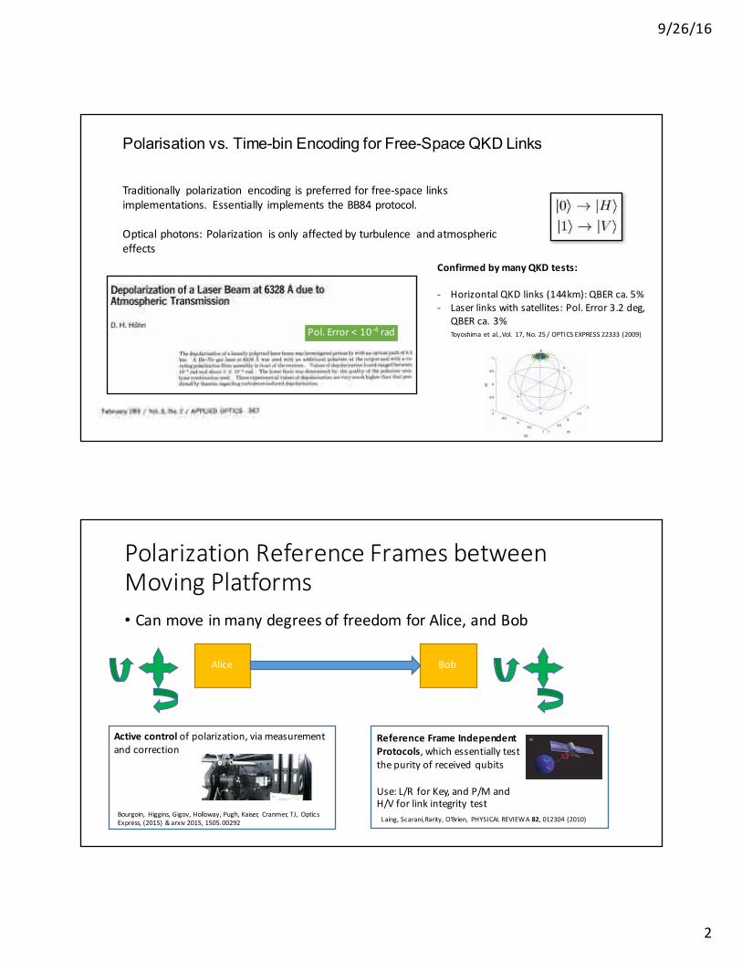
Polarisation vs. Time-bin Encoding for Free-Space QKD Links
Traditionally polarization encodingispreferredforfree-spacelinksimplementations. EssentiallyimplementstheBB84protocol.
Opticalphotons:Polarization isonlyaffectedbyturbulence andatmosphericeffects
Depolarization of a Laser Beam at 6328 A due toAtmospheric Transmission
D. H. Hhn
The depolarization of a linearly polarized laser beam was investigated primarily with an optical path of 4.5km. A He-Ne gas laser at 6328 A was used with an additional polarizer at the output and with a ro-tating polarization filter assembly in front of the receiver. Values of depolarization found ranged between10-7 rad and about 5 X 10- rad. The lower limit was determined by the quality of the polarizer-ana-lyzer combination used. These experimental values of depolarization are very much higher than that pre-dicted by theories regarding turbulence-induced depolarization.
I. IntroductionThe results of an experimental study of the depolar-
ization of a linearly polarized laser beam traversing theatmosphere near ground level are presented and dis-cussed in this paper.
A theoretical prediction, probably the first one con-cerned with turbulence-induced polarization fluctua-tions, was published by Hodara, but his results were inerror by some orders of magnitude,2 even if actualmeasurements2 seemed to confirm his theory. Friedand Mevers3 found very high degrees of polarizationfluctuations experimentally but "now it seems that thisrather large measured value was mainly due to a defect inthe experiment." 4 Strohbehm and Clifford5 presented anew theory on turbulence-induced polarization fluctua-tions. A first order solution to the wave equation wasfound using spectral analysis techniques. Finally, Saleh4
published a theory on polarization fluctuations usingthe geometrical optics approximation and Chernov'sthree-dimensional ray statistical model, together withsome experimental results. The sensitivity of hismeasurements was limited by the equipment used, to-42 dB in the daytime and -45 dB at night. Nodepolarization-corresponding to time- or space-aver-aged fluctuations of the polarization angle of a linearlypolarized laser beam-was found at a propagationrange of 2.6 km. In agreement with his theory, it mustbe much smaller as long as turbulence is the only sourceof depolarization.
Because of the fact that the above-mentioned theoret-ical predictions are contradictory, which is shown in
The author is with the Astronomisches Institut der UniversitdtTdbingen, Waldhauserstrasse 64, Ttibingen 74, Germany.
Received 6 August 1968.
Sec. II, the results of the measurements made nearTilbingen should not be compared directly with any onetheory, but should be discussed in light of the theoreticalsituation at present. In the Tubingen experiments, arange of 4.5 km was usually used. The experimentswere conducted at night from the middle of 1966 untilthe middle of 1967. Using a rotating-filter methodsimilar to that used by Saleh,4 depolarizations werefound. The root-mean-square variation of the angle ofpolarization a,, used as a parameter for the depolariza-tion, is compared with the root-mean-square variationof the logarithm of intensity slog ,, from which the struc-ture constant of the index of refraction C. can be de-duced; C. is a characteristic parameter of atmosphericturbulence.6
11. Theoretical ResultsA. Polarization Fluctuations
If the laser beam is polarized linearly at the trans-mitter output, the root-mean-square variation a-,, of theangle of polarization 0 induced by atmospheric turbu-lence is given by
1 (An2)'/2 l= - >,) 1'/2 (1)
if we follow the theory of Strohbehm and Clifford [Ref.5, Eq. (9) ]. An is the deviation of the index of refrac-tion of the atmosphere from its mean, normalized tounity; is the scale factor of the gaussian approxima-tion of the three-dimensional spectral density of theindex of refraction used, and may be considered to bethe correlation length [Ref. 5, Eq. (31) ]; X is the wave-length; L is the range of propagation. Assuming An2
= 10-12 and = 10 cm, corresponding to strong tur-bulence near the ground, we find when X = 632.8 nm
February 1969 / Vol. 8, No. 2 / APPLIED OPTICS 367
Pol.Error<10-4 rad
ConfirmedbymanyQKDtests:
- HorizontalQKDlinks(144km):QBERca.5%- Laserlinkswithsatellites:Pol.Error3.2deg,
QBERca.3%Toyoshimaetal. ,Vol. 17,No.25/OPTICSEXPRESS22333 (2009)
Fig. 6. Polarization characteristics of the downlink laser beam from the satellite. The blue, green and red dots show the data when the optical powers were received at −39 to −35, −41 to −39 and −43 to −41 dBm, respectively.
Figure 5 shows the Stokes parameters of (S1, S2, S3) measured during the experiment. The Stokes parameters with rms errors were measured as (S1, S2, S3) = (−0.054±0.109, −0.005±0.104, 0.987±0.009), which indicates circular polarization. Figure 6 shows the polarization characteristics on the Poincaré sphere. The rms angular error on the Poincaré sphere was measured to be within 3.2° in this experiment. One revolution of 360° on the Poincaré sphere experiences 180° in the rotation angle of the polarization; therefore, the rms angular error for the linear polarization becomes half of 3.2°. This value includes both the nature of the atmospheric slant path and the instrument error; however, if we calculate tan(3.2°/2) = 0.028, the cross leak component of the orthogonal polarization will be 2.8% from the main component, which can be considered as a quantum bit error rate (QBER) for QKD. In the past polarization measurements of a laser beam after propagation over a horizontal 144 km path, the QBER was measured to be 4.8 ± 1% which was caused by the various imperfection of their experimental setup [29]. In this paper, however, it was measured from space so the beam went through many different atmospheric layers in contrast to Ref [29]. According to QKD theory, the maximal tolerated error has an upper bound of 11% [30]. Therefore, the error budget can be considered to be within this maximal tolerated error for the satellite-to-ground QKD systems. Thus, it is useful to estimate the link budget for satellite-to-ground QKD scenarios by using the results presented here.
5. Conclusion
The polarization characteristics of an artificial laser source in space were measured through space-to-ground atmospheric transmission paths. A LEO satellite and an optical ground station were used to measure Stokes parameters and the degree of polarization of the laser beam transmitted from the satellite. The polarization was preserved within an rms error of 1.6°, and the degree of polarization was 99.4±4.4% through the space-to-ground atmosphere. These results contribute to the link estimation for QKD via space and provide the upper bound based on the measurements and the potential for enhancements in quantum cryptography worldwide in the future.
#116621 - $15.00 USD Received 2 Sep 2009; revised 9 Nov 2009; accepted 11 Nov 2009; published 23 Nov 2009(C) 2009 OSA 7 December 2009 / Vol. 17, No. 25 / OPTICS EXPRESS 22339
PolarizationReferenceFramesbetweenMovingPlatforms• CanmoveinmanydegreesoffreedomforAlice,andBob
Alice Bob
Activecontrolofpolarization,viameasurementandcorrection
ReferenceFrameIndependentProtocols,whichessentiallytestthepurityofreceivedqubits
Use:L/R forKey,andP/MandH/Vforlinkintegrity test
Bourgoin, Higgins,Gigov,Holloway,Pugh,Kaiser, Cranmer,TJ, OpticsExpress, (2015)&arxiv 2015,1505.00292
PHYSICAL REVIEW A 82, 012304 (2010)
Reference-frame-independent quantum key distribution
Anthony Laing,1,* Valerio Scarani,2,† John G. Rarity,1,‡ and Jeremy L. O’Brien1,§1Centre for Quantum Photonics, H. H. Wills Physics Laboratory & Department of Electrical and Electronic Engineering,
University of Bristol, BS8 1UB, United Kingdom2Centre for Quantum Technologies and Department of Physics, National University of Singapore, Singapore
(Received 18 March 2010; published 7 July 2010)
We describe a quantum key distribution protocol based on pairs of entangled qubits that generates a securekey between two partners in an environment of unknown and slowly varying reference frame. A direction ofparticle delivery is required, but the phases between the computational basis states need not be known or fixed.The protocol can simplify the operation of existing setups and has immediate applications to emerging scenariossuch as earth-to-satellite links and the use of integrated photonic waveguides. We compute the asymptotic secretkey rate for a two-qubit source, which coincides with the rate of the six-state protocol for white noise. We givethe generalization of the protocol to higher-dimensional systems and detail a scheme for physical implementationin the three-dimensional qutrit case.
DOI: 10.1103/PhysRevA.82.012304 PACS number(s): 03.67.Dd, 03.65.Ud, 03.67.Hk
I. INTRODUCTION
Technologies based on the principles of quantum in-formation [1] promise a revolution in informational taskssuch as computer processing [2,3] and communication [4].Secure communication via quantum key distribution (QKD)is one quantum information application that can be realizedwith current technologies [5–8]. In general, all the QKDprotocols proposed to date have in common the need for ashared reference frame between the authorized partners Aliceand Bob: alignment of polarization states for polarizationencoding, interferometric stability for phase encoding. Thisrequirement can, in principle, be dispensed with by encodinglogical qubits in larger-dimensional many-photon physicalsystems [9]. However, the creation, manipulation, and de-tection of many-photon entangled states is both technicallychallenging and very sensitive to the losses on the Alice-Bobchannel—in a word, impractical. More feasible single-photonphysical implementations have been proposed which seekto address the alignment limitations of standard protocols[10–13] yet these schemes can inherit further complica-tions that require active compensation between parties [14].To date, therefore, all practical implementations of QKDwithin an environment of varying phase have required theframes of Alice and Bob to be actively aligned by classicalcommunication.
In this paper, we present a reference frame independent(rfi) protocol that is separate from any particular physicalimplementation, can be implemented with ordinary sourcesand operate without frame alignment, beyond the obviousestablishment of a particle delivery link. Moreover, there areat least two emerging scenarios in QKD that will benefitfrom an rfi implementation (Fig. 1). The first such scenariois earth-to-satellite QKD [10,14–21]. In this case, one axisof the reference frame is well defined: The beam must
*[email protected]†[email protected]‡[email protected]§[email protected]
obviously connect the earth station with the satellite. Onthis beam, information encoded in circular polarization isvery stable, but the linear polarizations may vary in timebecause the satellite may be rotating with respect to the groundstation. The second scenario is path-encoded chip-to-chipQKD. The monolithic structures of planar waveguides havebeen successfully used to perform the stable interferometricmeasurements required in time and phase-encoded QKD[22–25]. More recently, integrated quantum photonic circuitshave demonstrated their potential as components for more
(a)
(b)
FIG. 1. (Color online) Two meaningful scenarios for referenceframe independent QKD. (a) Polarization encoding in earth-to-satellite quantum communication. Here the circular polarizationstates are stable, but the linear states can vary with the rotation of thesatellite. (b) Path encoding in chip-to-chip quantum communication.While the path information is stable, the unpredictable wavelength-scale changes in relative path length amount to a varying referenceframe. This may occur between chips communicating through freespace, or between chips connected by optical fibres.
1050-2947/2010/82(1)/012304(5) 012304-1 ©2010 The American Physical Society
Laing,Scarani,Rarity,O’Brien, PHYSICALREVIEWA82,012304 (2010)

9/26/16
3
CanadianQuantumSatelliteStudies
• QEYSSat• Missionproposal fora
micro-satellitequantumreceiver• IQCscientific lead• DesignedwithCanadian Industry• LEO• Mass:50kg,• Dimensions:80×60×60cm^3
• Status: Feasibility studies, missionandpayloaddevelopment (STDP),Form-fit-functionprototype+radtests, outdoor trials
• NanoQEY:• Cencept foraNano- Satbased
QuantumKeyExchangesatellite• Mass:15kg,• Dimensions:40×26×20cm^3
6-state
PAD
Beacon850 nm
NC
Tracking sensor + Feedback
switch WCP
Data Storage & Processing
Classical Comms
Classical comsOptical or RFQuantum signals
785 nm
FPM(AO)
Timing information retrieved from beacon
PolComp
DM
GPS timing, frequency and
location
QRx
Pol Analyzer + Detectors
Timing Electronics
Beacon
(Data Storage)
(Data Processing)
Classical Comms
Tracking + Feedb
λ Beacon
4-state
λ Quantum GPS
LinkAnalysis:J.P.Bourgoin,etal,NJP,15:023006,(2013)QYESSAT:T.Jenneweinetal,,volume8997ofProceedingsof SPIE,(2014).NanoQEY:T.Jenneweinetal,vol. 9254of Proceedingsof SPIE,(2014).
OutdoorTrialswithMovingTruck
0 1 2 3 4 5 6 7 8 90
10
20
30
40
50
60
70
80
90
100
Time [s]
QBE
R a
t rec
eive
r [%
] &R
aw k
ey [c
ount
s/2m
s]
Signal state QBERDecoy state QBERRaw key rate
Beaconacquiredby Alice
Beaconacquiredby Bob
QuantumtruckBourgoin, Higgins,Gigov,Holloway,Pugh,Kaiser, Cranmer,TJ, OpticsExpress, (2015)&arxiv 2015,1505.00292
FREE-SPACE QUANTUM KEY DISTRIBUTION TO A MOVING RECEIVER 15
0 1 2 3 4 5 6 7 8 9−1.5
−1
−0.5
0
0.5
1
1.5
Time [s]
Angu
lar sp
eed [
° /s]
Alice ∆ωazimuthAlice ∆ωelevationBob ∆ωazimuthBob ∆ωelevation
0.7°/s
Figure 6. Angular speed of the motors during the30 km/h test. The gray dotted line represents the max-imum angular speed of a 600 km LEO satellite (0.7 �/s).The higher variation at the receiver (Bob) is due to jitterand curving motion of the truck. The azimuthal angularspeed at the transmitter (Alice) is more consistent, withonly a small increase (of ⇡0.03 �/s) during the test. Be-fore 1.6 s Alice’s motors are not moving because she hasyet to acquire Bob’s beacon signal.
This operation represents di↵ering losses in the H and V modes, and isthus non-unitary. Because we are only concerned with the propertiesof states that are ultimately measured, we renormalize to impose unittotal probability in both modes via the N
mod
factor. Note that thisfactor is dependent on the state at this stage.
Because the interferometer cannot directly produce H and V, butonly states on the Bloch circle passing through D, A, R and L, a unitaryrotation operation is then applied to the state to transform R to H and
• 1stgenerationsystem• Quantumtransmissionrange650m• Quantumreceiver truckdriving30km/h• Generated160bitsecurekey• Realtime compensationofpointing,
polarizationandtiming

9/26/16
4
PhysicalParametersIOA Detectors CDPU Overall
Volume Budget 150 × 150 × 200 mm 150 × 150 × 200 mm
Measured 48.2 × 56.8 × 120 mm 30 × 127 × 143 mm 25.4 × 106.6 × 118.4
mmMass Budget (3 kg) (5 kg) (4 kg) 12 kgMeasured 0.32 kg 0.516 kg 0.129 kg < 2 kg
Power Budget (2.5 W) (2.5 W)* 6 W*
Measured 2.46 W 4 W* 6.46 W*
7
OpticalFinePointing
8
QBER[%] Countrate[/s]
Keyin100s[bits]• IntrinsicsourceQBER≈2%• NearconstantQBERoverfull
FOV(0.7deg)• Countratedropsattheedges,
reducingkeylength
9/26/16
5
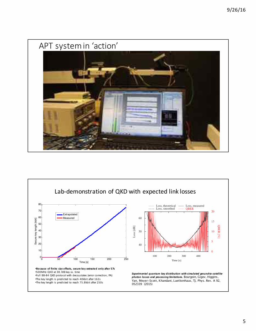
APTsystemin‘action’
Lab-demonstrationofQKDwithexpectedlinklosses
•Becauseoffinitesizeeffects,securekeyextractedonlyafter57s•500MHzQKDat38.7dBkeyvs.time•FullBB-84QKDprotocolwithdecoystates(errorcorrection,PA)•Thekeylengthispredictedtoreach40kbitafter162s•Thekeylengthispredictedtoreach75.8kbitafter250s
0 50 100 150 200 2500
10
20
30
40
50
60
70
80
Time [s]
Secu
re k
ey le
ngth
[kbi
t]
ExtrapolatedMeasured
Experimentalquantumkeydistributionwithsimulatedground-to-satellitephotonlossesandprocessinglimitations.Bourgoin, Gigov, Higgins, Yan, Meyer-Scott, Khandani, Luetkenhaus, TJ, Phys. Rev. A 92, 052339 (2015)
8
20
40
60
80
0 500 1000 1500 2000 2500
Loss
[dB
]
Time [s]
Loss, measuredLoss, smoothed
FIG. 6. Experimentally measured loss over the 45 min data collectionused to simulate the varying loss of a satellite pass. The data aresmoothed by taking the median value of a 29 s moving window.These smoothed values are used to select experimental data thattracks the theoretical loss of a satellite pass while maintaining thenatural statistical fluctuations.
into 1 s blocks, with the measured loss for each second overthe duration of the experiment shown in Fig. 6.
We redistribute select 1 s blocks of raw key data in sucha way that we obtain data sets that reproduce the statisticsexpected for real satellite uplink orbits [19]. The passes con-sidered are the best, upper-quartile and median passes (in termsof contact time) over a hypothetical ground station located at45° latitude of a year-long 600 km circular Sun-synchronouslow Earth orbit. The predicted losses are based on uplink ata wavelength of 785 nm, with a receiver diameter of 30 cm,a 2 µrad pointing error and a rural sea-level atmosphere. Thedi�erences with our system (which has 532 nm wavelength and5 cm receiver diameter) are necessary to mitigate the increasedgeometric losses over the long distance link of a satellite (re-quiring larger receiver diameter) and the e�ect of atmosphericturbulence and transmission (reduced at 785 nm compared to532 nm). Both our 532 nm system and the expected 785 nmsystem utilize the same Si avalanche photodiode technology.Analyzing our experimental data possessing these theoreticallosses is therefore a valid proof-of-concept demonstration.
The experimental data are smoothed by taking the median ofa moving window of 29 s width, the result illustrated in Fig. 6.We use these smoothed data to select 1 s experimental datablocks to include in our analysis for each orbit by progressivelyscanning (from the center, in either direction) in 1 s steps forthe next 1 s data block that possesses smoothed loss matchingor exceeding the theoretical orbit loss prediction. By selectingexperimental data at points where the smoothed loss is matchedto theoretical link predictions, we ensure that the data wesample are not biased by normal fluctuations in measured loss.
Figure 7 shows the three relevant losses—the theoreti-cally predicted loss, the smoothed loss value at the sampledpoint, and the experimentally measured loss from the sampledpoint—and the estimated QBER for each representative pass.The measured losses of the sampled experimental data closelymatch the trend of the theoretical prediction, whilst maintain-
50
60
70
100 200 300 4000
5
10
15
20
Loss
[dB
]
Time [s]
QB
ER[%
]
40
50
60
0
5
10
15
20
Loss
[dB
] QB
ER[%
]
40
50
60
0
5
10
15
20
Loss
[dB
] QB
ER[%
]
Loss, theoreticalLoss, smoothed
Loss, measuredQBER
FIG. 7. QBER and channel loss of data sets reconstructed frommeasured data (shown in Fig. 5) for three representative satellitepass conditions: best pass (top), upper-quartile pass (middle), andmedian pass (bottom). The predicted loss is based on an uplinkwith a 600 km circular Sun-synchronous low Earth orbit satelliteat a wavelength of 785 nm, with a receiver diameter of 30 cm, a2 µrad pointing error and a rural sea-level atmosphere. Smoothed lossfollows the moving median determined at each 1 s experimental datablock selected. Measured loss and QBER derive from the selecteddata, with shaded regions indicating the QBER 95 % credible intervalbased on a uniform Bayesian prior. For the best pass, we obtain3374 bit of secure key, including finite-size statistical e�ects.
ing realistic fluctuation. At higher losses the per-second QBERestimate has significant fluctuations due to the reduced samplesize.
Performing the post-processing steps on these data setsand incorporating finite-sized statistics, we are able to ex-tract a 3374 bit secure key from the best pass, out of a total of544 056 bit raw key (643 521 detection events) with an averageof 3.1 % QBER in the signal. This result shows that even withour modest 76 MHz source a positive key rate can feasibly begenerated from one pass (albeit a good one) of a typical lowEarth orbit satellite receiver. In comparison, the upper-quartile
8
20
40
60
80
0 500 1000 1500 2000 2500
Loss
[dB]
Time [s]
Loss, measuredLoss, smoothed
FIG. 6. Experimentally measured loss over the 45 min data collectionused to simulate the varying loss of a satellite pass. The data aresmoothed by taking the median value of a 29 s moving window.These smoothed values are used to select experimental data thattracks the theoretical loss of a satellite pass while maintaining thenatural statistical fluctuations.
into 1 s blocks, with the measured loss for each second overthe duration of the experiment shown in Fig. 6.
We redistribute select 1 s blocks of raw key data in sucha way that we obtain data sets that reproduce the statisticsexpected for real satellite uplink orbits [19]. The passes con-sidered are the best, upper-quartile and median passes (in termsof contact time) over a hypothetical ground station located at45° latitude of a year-long 600 km circular Sun-synchronouslow Earth orbit. The predicted losses are based on uplink ata wavelength of 785 nm, with a receiver diameter of 30 cm,a 2 µrad pointing error and a rural sea-level atmosphere. Thedi�erences with our system (which has 532 nm wavelength and5 cm receiver diameter) are necessary to mitigate the increasedgeometric losses over the long distance link of a satellite (re-quiring larger receiver diameter) and the e�ect of atmosphericturbulence and transmission (reduced at 785 nm compared to532 nm). Both our 532 nm system and the expected 785 nmsystem utilize the same Si avalanche photodiode technology.Analyzing our experimental data possessing these theoreticallosses is therefore a valid proof-of-concept demonstration.
The experimental data are smoothed by taking the median ofa moving window of 29 s width, the result illustrated in Fig. 6.We use these smoothed data to select 1 s experimental datablocks to include in our analysis for each orbit by progressivelyscanning (from the center, in either direction) in 1 s steps forthe next 1 s data block that possesses smoothed loss matchingor exceeding the theoretical orbit loss prediction. By selectingexperimental data at points where the smoothed loss is matchedto theoretical link predictions, we ensure that the data wesample are not biased by normal fluctuations in measured loss.
Figure 7 shows the three relevant losses—the theoreti-cally predicted loss, the smoothed loss value at the sampledpoint, and the experimentally measured loss from the sampledpoint—and the estimated QBER for each representative pass.The measured losses of the sampled experimental data closelymatch the trend of the theoretical prediction, whilst maintain-
50
60
70
100 200 300 4000
5
10
15
20
Loss
[dB]
Time [s]
QBER
[%]
40
50
60
0
5
10
15
20
Loss
[dB]
QBER
[%]
40
50
60
0
5
10
15
20
Loss
[dB]
QBER
[%]
Loss, theoreticalLoss, smoothed
Loss, measuredQBER
FIG. 7. QBER and channel loss of data sets reconstructed frommeasured data (shown in Fig. 5) for three representative satellitepass conditions: best pass (top), upper-quartile pass (middle), andmedian pass (bottom). The predicted loss is based on an uplinkwith a 600 km circular Sun-synchronous low Earth orbit satelliteat a wavelength of 785 nm, with a receiver diameter of 30 cm, a2 µrad pointing error and a rural sea-level atmosphere. Smoothed lossfollows the moving median determined at each 1 s experimental datablock selected. Measured loss and QBER derive from the selecteddata, with shaded regions indicating the QBER 95 % credible intervalbased on a uniform Bayesian prior. For the best pass, we obtain3374 bit of secure key, including finite-size statistical e�ects.
ing realistic fluctuation. At higher losses the per-second QBERestimate has significant fluctuations due to the reduced samplesize.
Performing the post-processing steps on these data setsand incorporating finite-sized statistics, we are able to ex-tract a 3374 bit secure key from the best pass, out of a total of544 056 bit raw key (643 521 detection events) with an averageof 3.1 % QBER in the signal. This result shows that even withour modest 76 MHz source a positive key rate can feasibly begenerated from one pass (albeit a good one) of a typical lowEarth orbit satellite receiver. In comparison, the upper-quartile

9/26/16
6
AirborneQKDwithquantumreceiver
Link Loss Estimation• Threshold for operation is grey
bar (43 dB)• Ground distance is path from
source to point on ground directly under plane
• Altitude is above ground not above sea level (however, atmosphere model is calculated at sea level so this is worst case)
• Shaded area is unusable as link loss is too high
10
Electronics Crate
• Dimensions 23”l x 21”w x 22.5”h• Needs to be located within 2 m of telescope.
4
2nd generationsystem:SatelliteprototypeonaircraftGoal:demonstrate quantumlinkwithupto1deg/s angularspeedAnalysisofair-speed,altitude,distance(graphonright)TestsconductedweekofSept.19th/2016
TheQuantumTransmitter setup QuantumReceiverPayloadIntegration&TestofPayloadataircraft
PolarizationIssueswithinOpticalSystems
Breckinridge, Lam, Chipman,Publicationsof theAstronomicalSocietyof thePacif ic,Vol.127,No.951(2015),pp.445
The depolarization coefficient k induced by thetelescope is 0.946. According to Eqs. (6) and (25),the measurement error of depolarization parameterda induced by the telescope is illustrated in Fig. 2 forwhen the telescope polarization crosstalk is not con-sidered. The error changes with the parameter da,
and a greater measurement error can be found whenthe depolarization parameter da becomes smaller.The maximum error can reach 5.7% when da is closeto zero.
B. Mueller Matrix of a Cassegrain Telescope
A Cassegrain telescope can be achieved by two mir-rors; a large concave paraboloidal primary with acentral hole, and a small hyperboloidal convex mir-ror. It is shown in Fig. 3.
If its focal length of the primary mirror is denotedby f 1, and the focal length of the second mirror is f 2,
the incident angles β1 on the primary mirror and β2on the second mirror can be expressed
β1 ≈ ρ∕!2f 1"; (26)
β2 ≈ ρ∕!2f 1" # $ρ!C · f 1 − f 2"%∕!2f 1f 2"; (27)
where C is the blocking ratio of the telescope.The corresponding rotation angles ofΩ1 andΩ2 can
be deduced according to the method in [14]
Ω1 & 0.5 arcsin!A · sin!αi" # B · sin!2αi""∕β21; (28)
Ω2 & 0.5 arcsin!A · sin!αi" # B · sin!2αi""∕β22 #Ω1:
(29)
A and B depend on the coordinate ρ, but they areindependent of α. The exact values of the coefficientsA and B does not matter.
A Cassegrain telescope with F number F & 3 isalso chosen as our simulated model. Its detail param-eters are shown in Table 2.
The Mueller matrix of the Cassegrain telescope inTable 2 is
MC &
0
BBB@
0.8517 −3.694 · 10−3 0 0−3.694 · 10−3 0.8517 −7.15 · 10−13 −1.6 · 10−14−2 · 10−15 7.15 · 10−13 0.8513 0.0273
0 0 −0.0273 0.8513
1
CCCA: (30)
When it is used in polarization lidar, the depolari-zation parameter da of aerosol is
da!z" &2I⊥
1.0087I∥ # I⊥. (31)
The induced depolarization coefficient is 1.0087.We also assume that the laser is aligned to theoptical axis of telescope. Similarly to Fig. 2 in theprevious section, the measurement error inducedby the Cassegrain telescope is shown in Fig. 4.The maximum measurement error is less than1%, even if the polarization crosstalk is notconsidered.
Fig. 2. Measurement error, induced by a Newton telescope withan aluminum coating, changes with the parameter da, and it has arange of 0–1; complex refractive index of the coating N is0.877# 6.479i.
Fig. 3. Sketch of a polarized ray path through a Cassegraintelescope.
Table 2. Parameters of the Cassegrain Telescope
Entrance pupil diameter D 667 mmFocal length f 2000 mmObscuration 187 mmf 1 −571.5f 2 −216.395N 0.877# 6.479i
20 January 2015 / Vol. 54, No. 3 / APPLIED OPTICS 393
2015/Vol.54,No.3/APPLIEDOPTICS
4. Polarization Effects and Correction of DifferentTelescopes
Besides coatings, the telescope’s Mueller matrix isrelated with system configuration and its character-istic parameters, such as curvature of reflector, Fnumber, and so on. Metal coating optical constantschange with wavelength [16], so a telescope’sMuellermatrix will change with wavelength. The Muellermatrices of a Newton telescope and a Cassegraintelescope coated with aluminum and silver were cal-culated over the wavelength range of 0.3–0.95 μm.The value of k changes with the parameters of thetelescope and laser wavelength.
Figures 5 and 6 show the curves of the depolariza-tion coefficient of a Newton telescope coated with analuminum and a silver layer in lidar applications,over the wavelength range of 0.3–0.95 μm. The val-ues of k change greatly with wavelength, and itreaches the extreme value at the wavelength of about0.83 μm for the aluminum layer, for the reasonthat there is the greatest optical constant of the
aluminum coating at 0.83 μm. From Fig. 7, the larg-est measurement error can be found at 0.83 μm. k iscalculated when the F number of the telescope is 2–8.The lesser value of k can be found in the telescopewith a lower F number, but the difference inducedby the F number is small and can be neglected.
The value of k pertinent to the silver coating is lessthan the aluminum coating over the wavelengthrange of 0.3–0.47 μm. There is a greater depolariza-tion coefficient of k at 0.47–0.95 μm for the silvercoating. At visible and near-infrared wavelengthsof 0.47–0.95 μm, there is less polarization crosstalkfor the silver coating.
The depolarization coefficients of a Cassegraintelescope with aluminum and silver coatings overthe wavelength range of 0.3–0.95 μm are shownin Fig. 8. For a Cassegrain telescope coated withaluminum, its depolarization coefficients are all ap-proximately equal to 1. That is to say, the depolari-zation of a Cassegrain telescope can be neglected inpolarization measurements of the atmosphere. For aCassegrain telescope coated with silver, there are
Fig. 4. Measurement error, induced by a Cassegrain telescopewith an aluminum coating, changes with the parameter da; ccomplex refractive index of the coatings N is 0.877! 6.479i.
Fig. 5. Calibration parameter of a Newtonian telescope coatedwith aluminum over the wavelength range of 0.3–0.95 μm (theF number of the telescope is 2–8); we assume that the laser polari-zation is aligned to the x axis in the coordinate system in Fig. 1.
Fig. 6. Depolarization coefficient of a Newtonian telescope coatedwith silver over the wavelength range of 355–950 nm; F number ofthe telescope is 2–8.
Fig. 7. Measurement error, induced by a Newton telescope withan aluminum coating, changes with the parameter da over thewavelength range of 0.28–0.83 μm.
394 APPLIED OPTICS / Vol. 54, No. 3 / 20 January 2015
PolarizationeffectofmirrorsduetoFresnel-coefficients
3.6 Reflections from Metal 83
3.6 Reflections from Metal
In this section we generalize our analysis to materials with complex refractiveindex N ¥ n + i∑. As a reminder, the imaginary part of the index controls atten-uation of a wave as it propagates within a material. The real part of the indexgoverns the oscillatory nature of the wave. It turns out that both the imaginaryand real parts of the index strongly influence the reflection of light from a sur-face. The reader may be grateful that there is no need to re-derive the Fresnelcoefficients (3.20)–(3.23) for the case of complex indices. The coefficients remainvalid whether the index is real or complex – just replace the real index n with thecomplex index N . However, we do need to be a bit careful when applying them.
Figure 3.10 The reflectances (top)with associated phases (bottom)for silver, which has index n = 0.13and ∑ = 4.05. Note the minimumof Rp corresponding to a kind ofBrewster’s angle.
We restrict our discussion to reflections from a metallic or other absorbingmaterial surface. As we found in the case of total internal reflection, we actually donot need to know the transmitted angle µt to employ Fresnel reflection coefficients(3.20) and (3.22). We need only acquire expressions for cosµt and sinµt, and wecan obtain those from Snell’s law (3.7). To minimize complications, we let theincident refractive index be ni = 1 (which is often the case). Let the index onthe transmitted side be written as Nt = N . Then by Snell’s law, the sine of thetransmitted angle is
sinµt =sinµi
N(3.45)
This expression is of course complex since N is complex, which is just fine.7 Thecosine of the same angle is
cosµt =q
1° sin2µt =1
N
q
N 2 ° sin2µi (3.46)
The positive sign in front of the square root is appropriate since it is clearly theright choice if the imaginary part of the index approaches zero.
Upon substitution of these expressions, the Fresnel reflection coefficients(3.20) and (3.22) become
rs =cosµi °
p
N 2 ° sin2µi
cosµi +p
N 2 ° sin2µi
(3.47)
and
rp =p
N 2 ° sin2µi °N 2 cosµip
N 2 ° sin2µi +N 2 cosµi
(3.48)
These expressions are tedious to evaluate. When evaluating the expressions, it isusually desirable to put them into the form
rs = |rs |ei¡s (3.49)
andrp =
Ø
ØrpØ
Øei¡p (3.50)
7See M. Born and E. Wolf, Principles of Optics, 7th ed., Sect. 14.2 (Cambridge University Press,1999).
SilverMirror:

9/26/16
7
AlternativeEncodingforQuantumInformationonFree-SpacePhotons?
• Inprinciple degreesoffreedom(D)F)ofphotonscanbeutilized toencodephotonic qubits• SpatialMode
• paths• Orbitalangularmomentum,LGmodes
• Timebin• related:DifferentialPhaseShift,COW
• Frequencybins,sidebands
• Quadratureoflight(onlycontinuous variables)
t2
Δτ
PBS
1
CC
4
3
a) entangledphoton source
b) hybrid quantum gate c) state analysis
FBS
Si-APD
coincidence logicQWPHWP Polarizer 45°fiber coupler CCCC
ψ+
(|HH〉+|VV〉)
2
fiber pol. controller adjustable delay
⊗|ω1ω2〉(|ω1ω2〉+|ω2ω1〉)
⊗|DD〉
ω2
ω1
FIG. 1: (Color online) Schematic of the experimental setup.(a) Source of polarization-entangled photon pairs with tun-able central frequencies. (b) The hybrid quantum gate’s po-larizing beam splitter (PBS) maps the polarization entangle-ment onto the color degree of freedom. Subsequently project-ing on diagonal (D) linear polarization with polarizers (POL)at 45◦ generates the discretely color entangled state. (c) Thestate is analyzed by two-photon interference at a fiber beam-splitter (FBS); Si-APD single-photon detectors and coinci-dence counting (CC) logic measure the coincidence rate as afunction of temporal delay between modes.
the resulting hypoentangled [26, 27] multi-DOF state:
|ψhypo⟩ = α|Hω1⟩3|Hω2⟩4 + eiφβ|V ω2⟩3|V ω1⟩4. (2)
To create the desired state, the frequency entanglementmust then be decoupled from the polarization DOF. Thiscan be achieved deterministically by selectively rotatingthe polarization of one of the two frequencies (e.g., us-ing dual-wavelength wave plates). For simplicity, we in-stead chose to erase the polarization information proba-bilistically by projecting both photons onto diagonal po-larization using polarizers at 45◦. We erased temporaldistinguishability between input photons by translatingfibre coupler 2 to maximise the non-classical interferencevisibility at the PBS for degenerate photons. Finally, wecompensated for unwanted birefringent effects of the PBSusing wave plates in one arm. The gate output is then:
|ψout⟩ = α|ω1⟩3|ω2⟩4 + eiφβ|ω2⟩3|ω1⟩4. (3)
The parameters defining this state can be set by prepar-ing an appropriate polarization input state (Eq. 1).
To explore the performance of the hybrid gate, wefirst injected photon pairs close to the polarization state(|H⟩1|H⟩2−|V ⟩1|V ⟩2)/
√2 with individual wavelengths
811.9 nm and 807.3 nm. The gate should then ide-ally produce the discrete, anticorrelated color-entangledstate: |ψ⟩ = (|ω1⟩3|ω2⟩4−|ω2⟩3|ω1⟩4)/
√2. Figure 2a)
shows the unfiltered single-photon spectra of the two out-put modes, illustrating that each photon is measured ateither ω1 or ω2. This reflects a curious feature of dis-cretely colour-entangled states, that individual photons
805 810 81501
Wavelength [nm]In
t.[a
.u.]
a) ω2 ω1 3
4
01
c) Re[ρ]
−0.5
0
0.75
ω2ω2ω2ω1 ω1ω2ω1ω1ω1ω1
ω1ω2
ω2ω1
ω2ω2
−0.010.01
Im[ρ]
ω2ω2ω2ω1 ω1ω2ω1ω1ω1ω1
ω1ω2
ω2ω1
ω2ω2
−2 −1 0 1 2Time Delay [ps]
No
rm.
Sin
gle
sC
oin
cid
en
ces,
pc
0
0.2
0.4
0.6
0.8
1b(i)
0
0.2
0.4
0.6
0.8
1b(ii)
3
4
FIG. 2: (Color online) Analysis of the discretely color-entangled state. a) Single-photon spectra for modes 3 and4; frequency separation is 2.1 THz (4.6 nm). The observedwidth of each bin is limited by the single-photon spectrome-ter. b) Normalized (i) coincidence and (ii) singles count ratesas a function of delay in mode 4. The solid line in (i) is a fitof Eq. 5 to determine V and the phase φ. c) The estimatedrestricted density matrix: target-state fidelity, 0.891±0.003;tangle, 0.611±0.009; and purity, 0.801±0.004.
have no well-defined color and no photon is ever observedat “mean-value” frequency. This feature clearly distin-guishes our experiment from the continuous frequencyentanglement studied in earlier work [5, 21, 22].
Because the detuning, µ = 4.6 nm, is much larger thanthe FWHM bandwidth of the individual color modes of0.66 nm (0.30 THz; defined by the 10 mm nonlinear crys-tal), the two modes are truly orthogonal, making themgood logical states for a frequency-bin qubit. This or-thogonality also means that color anticorrelations arestrictly enforced by energy conservation, because a sin-gle down-conversion event cannot produce two photonsin the same frequency bin. We confirmed this by di-rectly measuring the gate output in the frequency-bincomputational basis (i.e. with bandpass filters in eacharm tuned to ω1 or ω2). We observed strong, compara-ble coincidence rates for the two “anticorrelated” basisstates (10882 ± 104 and 9068 ± 95 in 30s for |ω1⟩3|ω2⟩4and |ω2⟩3|ω1⟩4, resp.), and no coincidences for the same-frequency states (|ω1⟩3|ω1⟩4 and |ω2⟩3|ω2⟩4) to within er-ror bars determined by the filters’ finite extinction ratios.
To demonstrate that the color state was not only anti-correlated but genuinely entangled, we used nonclassicaltwo-photon interference [28], overlapping the photons ata 50:50 fibre beam splitter (FBS) (Fig. 1c) and vary-ing their relative arrival time by translating fibre cou-pler 4 while observing the output coincidences. The re-sults in Fig. 2b) show high-visibility sinusoidal oscilla-tions (frequency µ) within a triangular envelope causedby the unfiltered “sinc-squared” spectral distribution ofthe source [4, 29]. At the central delay, the normalisedcoincidence probability reaches up to 0.881 ± 0.007, far
the continuous-variable Clifford group can be efficientlysimulated by purely classical means. This is acontinuous-variable extension of the discrete-variableGottesman-Knill theorem in which the Clifford groupelements include gates such as the Hadamard !in thecontinuous-variable case, Fourier" transform or the con-trolled NOT !CNOT". The theorem applies, for example,to quantum teleportation which is fully describable byCNOT’s and Hadamard !or Fourier" transforms of someeigenstates supplemented by measurements in thateigenbasis and spin or phase flip operations !or phase-space displacements".
Before some concluding remarks in Sec. VIII, wepresent some of the experimental approaches to squeez-ing of light and squeezed-state entanglement generationin Sec. VII.A. Both quadratic and quartic optical nonlin-earities are suitable for this, namely, parametric downconversion and the Kerr effect, respectively. Quantumteleportation experiments that have been performed al-ready based on continuous-variable squeezed-state en-tanglement are described in Sec. VII.D. In Sec. VII, wefurther discuss experiments with long-lived atomic en-tanglement, with genuine multipartite entanglement ofoptical modes, experimental dense coding, experimentalquantum key distribution, and the demonstration of aquantum memory effect.
II. CONTINUOUS VARIABLES IN QUANTUM OPTICS
For the transition from classical to quantum mechan-ics, the position and momentum observables of the par-ticles turn into noncommuting Hermitian operators inthe Hamiltonian. In quantum optics, the quantized elec-tromagnetic modes correspond to quantum harmonicoscillators. The modes’ quadratures play the roles of theoscillators’ position and momentum operators obeyingan analogous Heisenberg uncertainty relation.
A. The quadratures of the quantized field
From the Hamiltonian of a quantum harmonic oscil-lator expressed in terms of !dimensionless" creation andannihilation operators and representing a single mode k,Hk=!"k!ak
†ak+ 12
", we obtain the well-known form writ-ten in terms of “position” and “momentum” operators!unit mass",
Hk =12
!pk2 + "k
2xk2" , !1"
with
ak =1
#2!"k!"kxk + ipk" , !2"
ak† =
1#2!"k
!"kxk − ipk" , !3"
or, conversely,
xk =# !
2"k!ak + ak
†" , !4"
pk = − i#!"k
2!ak − ak
†" . !5"
Here, we have used the well-known commutation rela-tion for position and momentum,
$xk,pk!% = i!#kk!, !6"
which is consistent with the bosonic commutation rela-tions $ak , ak!
† %=#kk!, $ak , ak!%=0. In Eq. !2", we see that upto normalization factors the position and the momentumare the real and imaginary parts of the annihilation op-erator. Let us now define the dimensionless pair of con-jugate variables,
Xk &#"k
2!xk = Re ak, Pk &
1#2!"k
pk = Im ak. !7"
Their commutation relation is then
$Xk,Pk!% =i2
#kk!. !8"
In other words, the dimensionless position and momen-tum operators, Xk and Pk, are defined as if we set !=1/2. These operators represent the quadratures of asingle mode k, in classical terms corresponding to thereal and imaginary parts of the oscillator’s complex am-plitude. In the following, by using !X , P" or equivalently!x , p", we shall always refer to these dimensionlessquadratures as playing the roles of position and momen-tum. Hence !x , p" will also stand for a conjugate pair ofdimensionless quadratures.
The Heisenberg uncertainty relation, expressed interms of the variances of two arbitrary noncommutingobservables A and B for an arbitrary given quantumstate,
'!$A"2( & Š!A − 'A("2‹ = 'A2( − 'A(2,
'!$B"2( & Š!B − 'B("2‹ = 'B2( − 'B(2, !9"
becomes
'!$A"2('!$B"2( %14
)'$A,B%()2. !10"
Inserting Eq. !8" into Eq. !10" yields the uncertainty re-lation for a pair of conjugate quadrature observables ofa single mode k,
xk = !ak + ak†"/2, pk = !ak − ak
†"/2i , !11"
namely,
'!$xk"2('!$pk"2( %14
)'$xk,pk%()2 =116
. !12"
Thus, in our units, the quadrature variance for a vacuumor coherent state of a single mode is 1 /4. Let us further
516 S. L. Braunstein and P. van Loock: Quantum information with continuous variables
Rev. Mod. Phys., Vol. 77, No. 2, April 2005
Free space quantum key distribution with coherent polarization states 6
Figure 3. Contour plots of the two coherent states in our binary phase shiftkeying protocol. The amplitude α corresponds to the first moment of the Gaussianprobability distributions. Due to the small amplitude the two states are nearlyindistinguishable to Eve. By postselecting favourable measurement events, Bobgains an information advantage over Eve [29].
split into two parts by a Wollaston prism. The difference of the photocurrents from thetwo photodiodes is electronically amplified and recorded. For an S2 measurement, thedetection basis is adjusted by a half-wave plate. Monitoring of the S3 component [39]is not performed in this study, but will be implemented in future experiments.
3. Results
We commence this section with an investigation of the noise behaviour of our newlydeveloped magneto-optical modulator. Next, we present measurements of atmosphericpolarization noise. From the absence of significant excess noise in both cases wededuce that our system is suitable for QKD operation. Finally, we demonstrate thetransmission of quantum states over the atmospheric channel and provide calculationsof the achievable key rate.
3.1. Noise behaviour of the magneto-optic modulator
The bandwidth of our magneto-optical modulator (MOM) is limited by the inductanceof the coil which generates the magnetic field. In the new version, the size of this coilhas been decreased which enables us to operate the modulator at 1MHz. Whencharacterizing the MOM, we detect the modulated beam directly after modulation.We are therefore able to investigate the noise behaviour of the MOM separately fromthe free space channel.
A signal state is generated by applying a predefined positive or negative voltageto the MOM driver for 400ns. After each signal pulse the modulation voltage isswitched to zero for 600ns to enable the modulator to return to its zero position.Furthermore, a vacuum reference is needed for calibration since the polarization inthe setup drifts slowly in time. We determine the vacuum level by taking into account100 vacuum measurements neighbouring each signal pulse. At a constant vacuumlevel, an increased number of calibration pulses allows for a more precise calibration.In practice, however, this number is limited by slow polarization drifts as well as bylaser excess noise at low frequencies.
We determine the excess noise of a signal state by comparing its variance tothe variance of the vacuum state (shot noise). The variance of the vacuum state isnormalized to unity. Figure 4 shows the excess noise introduced by the modulation
Are theysuitableforalongdistancefree-spacelink?Motionerrors,atmosphericturbulence
Timebinencodingforfree-space
• Requires,thattheunbalancedinterferometersforencoding/decodingthequbits canworkwithmultimodal beams
(left)Singlemodeban(right)Testbeamgenerated2mofMMF
3
light, a single-mode Gaussian with an amplitude of a and variance �
2, at the output of
interferometer as
I(�(↵),�) = ⇡a
2
�
2
1 + exp
�✓�(↵)
2�
◆2
!cos(�)
!, (2)
Here, � denotes the relative phase between the interfering paths. Combining the Eq. (1)
and Eq. (2) yields the visibility of interference V , defined by (Imax
�I
min
)/(Imax
+I
min
),
as
V(↵) = V0
exp
�✓
�l
0
tan(↵)p2�(1 + tan(↵))
◆2
!, (3)
where V0
denotes the system visibility at zero AOI. For instance, with � = 1.49mm and
�l
0
= 0.60m, chosen to achieve a clear separation of the time bins given our detector
timing jitter and channel-induced dispersion, we expect the visibility to drop to 0.70 for
↵ = 1.70mrad and V0
= 0.91. Furthermore, the relative phase between the two paths is
very sensitive to the AOI, with a predicted ⇡–shift per 349 nrad input angle variation.
The relationship Eq. (3) is verified experimentally with a single-mode beam (see
Fig. 1(a)), generated by a continuous-wave laser at 776 nm. For instance, as shown in
Fig. 1(d), the initial interference visibility of Vsingle
0
= 0.91 ± 0.01 decreases rapidly
with AOI when no correction optics are implemented, as expected from Eq. (3). Next,
the same laser beam is sent through a multimode fiber, thereby distorting it into a
multimodal beam [23] which mimicks the e↵ect of turbulent atmosphere (Fig. 1(b),
see [1, 17] for comparison). Despite lengthy and careful alignment we are only able to
obtain a maximum visibility of Vmulti
0
= 0.16 ± 0.01, which, as shown in Fig. 1(e), drops
with AOI. Current solutions to this behavior include spatial-mode filtering using single-
mode optical fibers, which, however, discard most of the impinging photons [24]. These
observations clearly show that, given the expected angular deviations reported for free-
space quantum channels, it would be technically very challenging to achieve a reliable,
stable and e�cient operation of time-bin qubit receiver using standard interferometers.
2.1. MM-TQA with imaging optics
These interference challenges are overcome by utilizing relay optics in the long arm of the
unbalanced Michelson interferometer, as shown in Fig. 1(c). E↵ectively, the relay optics
reverse di↵erences in the evolution of the spatial mode over length �l in the long arm,
and thus symmetrize the two paths of the interferometer while maintaining temporal
separation between the paths. With the TQA design, for a single-mode beam, an inter-
ference visibility of Vsingle
avg
= 0.91 ± 0.01 is obtained, which remains constant as the AOI
is varied (see Fig. 1(d)). The improvement is further confirmed by measurements with a
multimode beam (Fig. 1(b)) where the high visibility of Vmulti
avg
=0.89 ± 0.01 (Fig. 1(e))
demonstrates that the interferometer design is robust against highly distorted beams.
The output of the interferometer is coupled into a multimode fiber, with a coupling
e�ciency of 0.87, for delivery of the photons to the detector. The total throughput is
UncorrectedInterferometer:
PriorSolutions:Coupleintosinglemodefiber(lossesveryhigh)Adaptiveoptics(canbelossy,challenging)

9/26/16
8
Multi-modeMichelsonInterferometers
© 1995 Nature Publishing Group
Erskine,Holmes, Nature,Vol 377,p317 (1995)
US006115121A
United States Patent [19] [11] Patent Number: 6,115,121 Erskine [45] Date of Patent: *Sep. 5, 2000
[54] SINGLE AND DOUBLE SUPERIMPOSING S. Gidon and G. Behar, “Multiple—line laser Doppler veloci INTERFEROMETER SYSTEMS
[75] Inventor: David J. Erskine, Oakland, Calif.
[73] Assignee: The Regents of the University of California, Oakland, Calif.
[*] Notice: This patent is subject to a terminal dis claimer.
[21] Appl. No.: 08/963,682 [22] Filed: Oct. 31, 1997
[51] Int. Cl.7 ..................................................... .. G01B 9/02
[52] US. Cl. ........................ .. 356/345; 356/285; 356/352 [58] Field of Search ................................... .. 356/345, 346,
356/351, 352, 357, 359, 28.5
[56] References Cited
U.S. PATENT DOCUMENTS
5,642,194 6/1997 Erskine ................................. .. 356/345
OTHER PUBLICATIONS
Rernhard Beer, “Remote Sensing by Fourier Transform Spectrometry,” John Wiley & Sons, NeW York, 1992, QD96.F68B415, p. 17. P. Connes, “L’Etalon de Fabry—Perot Spherique,” Le Journal De Physique et le Radium, 19, pp. 262—269, 1958. R. L. Hilliard and G. G. Shepherd, “Wide Angle Michelson Interferometer for Measuring Doppler Line Widths,” J. Opt. Soc. Am., vol. 56, No. 3, pp. 362—369, Mar. 1966.
SM. 88,57 \\\\ AM.
90
metry,” Applied Optics, vol. 27, No. 11, pp. 2315—2319, 1988.
Pierre Connes, “DeuXieme Journee D’Etudes Sur Les Inter ferences,” Revue D’Optique Theorique Instrumentale, vol. 35, p. 37, Jun. 1956. Book by Eugene Hecht and Alfred Zaj ac, “Optics,” Addison Wesley, Reading Massachusetts, pp. 307—309, 1976. David J. Erskine and Neil C. Holmes, “White Light Veloc ity,” Nature, vol. 377, pp. 317—320, Sep. 28, 1995. David J. Erskine and Neil C. Holmes, “Imaging White Light VISAR,” Proceedings of 22nd International Congress on High—speed Photography and Photonics, October 1996.
Primary Examiner—Samuel A. Turner Attorney, Agent, or Firm—John P. Wooldridge; Alan H. Thompson [57] ABSTRACT
Interferometers Which can imprint a coherent delay on a broadband uncollimated beam are described. The delay value can be independent of incident ray angle, alloWing interferometry using uncollimated beams from common extended sources such as lamps and ?ber bundles, and facilitating Fourier Transform spectroscopy of Wide angle sources. Pairs of such interferometers matched in delay and dispersion can measure velocity and communicate using ordinary lamps, Wide diameter optical ?bers and arbitrary non-imaging paths, and not requiring a laser.
32 Claims, 34 Drawing Sheets
Delaying Mirror Assembly
Erskine,USPatent6,115,121 (2000)
SuperimposingInterferometers Field-WidenedMichelsonInterferometers
Liu etal,Vol. 20,No.2/OPTICSEXPRESS1406 (2012)
spectral filter also have large field of view, which means that the spread of incident angles may be relatively large (e.g., approximately 1° full-angle for the LaRC HSRL-2 instrument).
Expanding 0sinθ we get
2 1 21 1 2 2 0
1 2
4 6
0 01 2 1 2
3 3 5 5
1 2 1 2
2( ) sin ( )
,sin sin
( ) ( )4 8
d dW n d n d
n n
d d d d
n n n n
θ
θ θ
= − − −
− − − − ⋯⋯ (7)
and we can find that, the OPD is power series of the sine squared incident angle. In order to enlarge the field of view, we can let the second term be zero, that is
1 1 2 2/ / 0.d n d n− = (8)
Then this system would be independent of incident angle to third order and have an OPD between the two arms as
4 6
0 01 2 1 21 1 2 2 3 3 5 5
1 2 1 2
sin sin2( ) ( ) ( )
4 8
d d d dW n d n d
n n n n
θ θ= − − − − − ⋯⋯ (9)
where the 4th and higher terms can be omitted when θ is small. Note that one can obtain a super field-widened Michelson filter by adding more glasses [18].
Figure 3 shows the incident angle dependence of OPD for an ordinary Michelson interferometer (blue star) and a field-widened one (pink diamond) that has the same original OPD (150mm) and works at the same wavelength (355nm). As is shown in Fig. 3(a), the OPD suffers a change of more than 60 λ for the ordinary MI with the incident angle at 1 degree while the OPD of the field-widened MI is very constant over a large range of incident angle. Figure 3(b) shows a detail illustration of the incident angle dependence of the field-widened MI and the discussed field-widened MI encounters an OPD change of only about 0.068 λ . For a 400mm aperture, 1mrad field of view telescope, the spectral filter should have at least 16mrad if the input beam aperture is 25mm. The 16mrad divergence angle, or about 0.92 degree, is too large for ordinary MI to act as spectral filter, but it will not pose a problem for a field-widened MI.
Fig. 3. Comparison of OPD incident angle dependence between ordinary and field-widened Michelson interferometers, (a) incident angle dependence comparison, (b) detailed illustration of the performance of the field-widened MI.
2.3 Transmission ratio of the Michelson spectral filter
Figure 4 shows a schematic diagram of the field-widened Michelson spectral filter for spectral discrimination in HSRL system. The backscatter signal which contains backscatter from the
#156591 - $15.00 USD Received 17 Oct 2011; revised 28 Nov 2011; accepted 21 Dec 2011; published 9 Jan 2012(C) 2012 OSA 16 January 2012 / Vol. 20, No. 2 / OPTICS EXPRESS 1410
stable, and can obtain high quality spectral discrimination [4, 12, 13]; however, absorption filters are not photon efficient and there are no absorption lines at many convenient laser wavelengths. Field-widened interferometers [14, 15] are of high efficiency and can be built to any desirable laser wavelength. Applications, such as measuring Doppler linewidths [15], demonstrate they can be adopted as the interferometric spectral filter for HSRL system.
A compact, robust, quasi-monolithic tilted field-widened Michelson interferometer (MI) is under development as the spectral discrimination filter for a second-generation HSRL(HSRL-2) at National Aeronautics and Space Administration (NASA) Langley Research Center (LaRC). The MI consists of a cubic beam splitter, a solid arm and an air arm. Piezo stacks connect the air arm mirror to the body of the interferometer allowing the interferometer to be tuned within a small spectral range. The widened field of view makes the optical path difference (OPD) of the filter vary slowly with incident angle and allows the collection of light over a large angle. In this paper, the system performance is analyzed over several types of system imperfections, such as cumulative wavefront error, locking error, reflectance of the beam splitter and anti-reflection coatings, system tilt, and depolarization angle. The requirements of each imperfection for good interferometer performance are obtained.
This paper is constructed as follow: Section 2 makes a detailed description of the field-widened Michelson interferometric spectral filter and provides the definition of the Transmission Ratio that can be used to evaluate the performance of the Michelson spectral filter in HSRL; Section 3 shows the principle of the prototype tilted field-widened MI for HSRL; the system performances of the interferometer are analyzed over different system imperfections in Section 4, which is followed by discussions in Section 5, and finally, some conclusions are given in Section 6.
2. Field-widened Michelson spectral filter for HSRL
2.1 Michelson interferometer
The MI is one of the best known interferometers in optical testing and has been adopted for many applications [16, 17]. It consists of a 50/50 beam splitter and two arms with a mirror at each end. The input beam is directed into the system and produces two outputs, as are indicated by Output I and II in Fig. 2.
Fig. 2. Ray diagram of Michelson interferometer.
When the incident angle 0θ is zero, the above shown interferometer is an ordinary
Michelson interferometer and the irradiance IT at the Output I can be expressed as
0 0 02 [1 cos 2 ]IT I t r Wπ= + (1)
where, 0I is the irradiance of input beam, 0t and 0r are the absolute transmittance and
reflectance coefficients of the beam splitter and W is the OPD of the two arms in the unit of wavelength.
In a similar way, the irradiance IIT at the Output II is
#156591 - $15.00 USD Received 17 Oct 2011; revised 28 Nov 2011; accepted 21 Dec 2011; published 9 Jan 2012(C) 2012 OSA 16 January 2012 / Vol. 20, No. 2 / OPTICS EXPRESS 1408
Usedinapplicationsformulti-modeimagesinDoppler-LIDARVelocimetrywithincoherentlightsources,Astronomy,NarrowbandFiltersinLIDAR
Appl. Opt.24(11),1571–1584 (1985)Appl. Opt.11(3),507–516(1972).
Unbalanced InterferometerSuitableforQuantumCommunications• CompatibilitywithPhotonicQubits:
• Dispersion,Polarizationeffects,stability?
- [J. Jin,S. Agne, J.P.Bourgoin,Y.Zhang,N.Lutkenhaus,T.Jennewein, arXiv:1509.07490]ZEMAXmodellingofopticalconfiguration

9/26/16
9
DemonstrationusingEntangledPhotons 7
LASER!!404 nm
776 nm (A)
842 nm (B)
PQA EPS
time coin
ciden
ce
Time tagger
Multimode Channel
Multimode Channel
MM-TQA1
MM-TQA2
TQC1
TQC2 D2
PQA for source visibility
D1
Method 1
Method 2
AOI (α)
AOI (α)
HWP
QWP
BPF
POL
DM
FM
M
Lens
PBS
BS
FPC Glass
Si-APD PPKTP
SMF
MMF
T1
T1
Figure 2. Experimental setup. The polarization-entangled photon-pair source(EPS) is described in the text. For projection measurements, photon A is directed to apolarization-qubit analyzer (PQA), consisting of a quarter-wave plate (QWP), a half-wave plate (HWP), a polarizing beam splitter (PBS), and silicon avalanche photodiodes(Si-APDs). After reflection at a dichroic mirror (DM), by a flip mirror (FM), photonB is sent either to a PQA or a time-bin qubit converter (TQC1(2)) followed bya multimode fiber and a multimode time-bin qubit analyzer (MM-TQA1(2)). Thepurpose of the PQA is to measure reference entanglement visibilities with the source ofpolarization entanglement, which will be compared to visibilities with polarization-timeentanglement. The TQC maps the polarization qubit onto a time-bin qubit (see textfor details). For projection measurements, the time-bin qubit, spatially and temporallydistorted by a multimode fiber (MMF), is then sent to a MM-TQA whose output iscoupled into a MMF before detection by a Si-APD. A polarizer (POL) removes anypossible path-dependent polarization distinguishability. All detection signals are sentto a time tagger for data analysis.
variable AOI within experimental errors, confirming the robustness of the MM-TQAs
against angular fluctuations.
3.2.3. Phase invariance against AOI variation Without correcting optics, a variance
of AOI also introduces phase fluctuations of interferometer [26]. From our theoretical
model, we anticipate a 5⇡-shift with an AOI of only 1.75 µrads (see inset of Fig. 4). To
assess the phase stability of the MM-TQA with AOI, using the method 1, we measure
expectation values, defined as E�
⌘ (N+�
0�
�N��
0�
)/(N+�
0�
+N��
0�
), for AOIs changing
from -0.20� to +0.20� continuously over 20 seconds. The measured E-values remain
almost constant within experimental errors (see Fig. 4), showing that the MM-TQA
5
0.74 from input to output.
2.2. MM-TQA with di↵erent refractive-indexed paths
The second method we studied is to use di↵erent refractive-indexed medium for
each path of an unbalanced interferomter [20]. The optical path di↵erence of the
interferometer is given by �l = 2(nL
l
L
cos✓
L
� n
S
l
S
cos✓
S
), where n
L(S)
denotes the
refractive index of the path l
L(S)
. Using Snell’s law and Taylor’s expansion, the di↵erence
can be approximated as 2(nL
l
L
� n
S
l
S
)� sin
2
✓(lL
/n
L
� l
S
/n
S
) for small angles ✓L
and
✓
S
. By properly choosing refractive indices for the paths, one can remove the second
term so that �l becomes insensitive to AOI. In our implementation (see Fig. 1(f)), we
use a 118 mm-long glass with the refractive index of 1.4825 in the long path and none
in the short path, providing an optical path-length di↵erence of 0.57 ns. Interference
visibilities of 0.94±0.01(see Fig.1(g)) and 0.90±0.01 (see Fi.g 1(h)) are measured with
a single-mode and multimode beam respectively, which remain constant with various
AOI within experimental errors. For the used glass, we calculated dispersion of 5.48
waves/nm and 5.21 waves/ �C. In order to avoid the dispersion e↵ect, we symmetrize
the paths in the time-bin converter and analyzer as shown in Fig. 2.
3. Demonstration of MM-TQAs for quantum communication
3.1. Experimental setup
The utility of the interferometers, as working TQAs for multimodal quantum signals, is
demonstrated with the experimental setup depicted in Fig. 2. Light from a 404 nm
continuous-wave laser with an average power of 6mW pumps a periodically poled
potassium titanyl phosphate crystal inside a Sagnac interferometer. This generates
polarization entangled photon pairs at 776 nm (A) and 842 nm (B) in a form of
| i = 1p2
(|ViA
|HiB
+ |HiA
|ViB
) via a type-II spontaneous parametric downconversion.
Here, |Hi and |Vi is the horizontal and vertical polarization state respectively, forming
the eigenstates of the computational basis. Unused pump photons are removed by
band-pass filters. While the photon B is directed to a polarization analyzer, the photon
A is sent either a polarization analyzer or a time-bin converter (TQC) followed by a
multimode channel and a MM-TQA for various measurements.
To convert a polarization state of the photon A into a time-bin state, we use an
unbalanced interferometer as a TQC1(2)
, whose path-length di↵erence is matched to the
MM-TQA1(2)
. At the polarizing beam splitter of the TQCs, the photon is either reflected
or transmitted into the short or long path, respectively. A fiber-polarization controller
ensures the faithful mapping of the vertical (horizontal) polarization onto the early (late)
temporal bin. The inserted quarter-wave plate in each path guides the photon to the
desired output port. Leaving the TQCs, the photon passes through a polarizer set to an
equal superposition between the polarizations, allowing to erase polarization information
6
for each time-bin states at the cost of 50 % transmission loss. This therefore completes
the map |Vi 7! |Ei and |Hi 7! |Li, resulting the two-photon entangled state in the
hybrid state
| i = 1p2(|Ei
A
|HiB
+ |LiA
|ViB
), (4)
where |Ei (|Li) denotes the quantum state in which photon A is in early (late) temporal
mode. The photon A then travels through a 1m-long step-index multimode fiber, as
a multimode channel, distorting the spatial mode (see Fig. 3(a)) and temporal mode
(measured dispersion is about 50 ps, drastically exceeding the photon’s coherence time
of of 3.2 ps [25]), prior to entering the MM-TQAs. After being analyzed in the MM-
TQAs, both photon A and B are detected by silicon avalanche photodiodes and the
detection signals are sent to a time tagger and a computer for data analysis.
3.2. Experimental results
3.2.1. Observation of Entanglement Verification of the MM-TQA performance is done
by measuring entanglement visibilities. Each qubit is first projected onto computational
basis, i.e. | ± Zih±Z|, where | + ZiA
⌘ |Ei, | � ZiA
⌘ |Li, | + ZiB
⌘ |Hi,and | � Zi
B
⌘ |Vi. The coincidence counts are used to calculate visibilties V±z
⌘(N±z±z
�N⌥z±z
)/(N±z±z
+N⌥z±z
), from which we obtain the average Vz
= (V+z
+V�z
)/2.
Here, Nij
denotes the joint-detection counts when time-bin qubit A is projected onto
|iihi| and polarization qubit B onto |jihj|, where i, j 2 {+Z, -Z} (see Fig. 3(b)). More
important operation is the projection of the time-bin qubits onto superposition states,
i.e. | ± �ih±�|, where | ± �iA(B)
⌘ 1p2
(| + ZiA(B)
± ei�A(B) | � ZiA(B)
). To measure the
visibility, we vary the relative phase between basis states of the polarization qubit. A
complete scan of the phase along the xy-plane of the Bloch sphere is performed, yielding
an average visibility Vxy
= (V+xy
+ V�xy
)/2 (see Fig. 3(c)). These allow to compute
an average visibility as Vavg
⌘ Vz
/3 + 2Vxy
/3. In order to access the performance
of the MM-TQAs, we compare the value to source visibility obtained from original
polarization entanglement. This is done by routing the photon A to a polarization
analyzer. For the method 1(2), we measure visibilities of Vz
=0.95 ± 0.01 (0.92 ± 0.01)
and Vxy
=0.80 ± 0.01 (0.77 ± 0.01), yielding an average visibility of Vavg
= 0.85 ± 0.01
(0.82 ± 0.01). Di↵erence from a source visibility of Vref
avg
=0.93 ± 0.01(0.91 ± 0.01), as
shown in Fig. 3(d), mainly stems from non-perfect projection of time-bin qubit onto
superposition bases.
3.2.2. Tolerance to angular fluctuations To prove the invariance of interfering power of
the MM-TQAs against AOI variation of incoming photon, we carry out the entanglement
verification measurements for di↵erent AOI. Due to the coupling geometry of the photons
into the multimode detector fiber, we vary the AOI up to 3.49 mrads. Note that the
value is larger than measured error of our signal pointing system on a moving vehicle [22].
As shown in Fig. 3(d), for the both methods, the measured visibilities are constant to
HybridentangledState:
Xiao-song Ma, et al, PHYSICAL REVIEW A, 79(4), (2009).
Type-Iinterferometer, relay lensTimedelay:2ns
ExperimentalTestofHybridEntanglement
8
AOI (degrees)
Enta
ngle
men
t vis
ibility
0.05 0.10 0.15 0.2000
0.2
0.4
0.6
0.8
1
Phase(radian)
0
30
280
Sin
gle
counts
(kH
z)C
oin
cid
ences (
Hz)
Norm
aliz
ed c
oin
cidence
s
Time (ns)
0
0.2
1
0 3 6 9 12 15 18 21
-Z +Z +Z -Z
-Z -Z
Z
Y
X2 mm
210
140
70
60
90
120
2 4 6
0.4
0.6
0.8
Lens-assisted TQA
Glass-assisted TQA
ϕ'+ϕ'
-ϕ'
+Z +Z (d)(a) (b)
(c)
Figure 3. Experimental results for entangled photons analyzed with MM-
TQAs. (a) Spatial mode of the photon A before entering the MM-TQA. The imageis captured by a Hamamatsu electron multiplier CCD camera (C9100-13). (b) Jointdetections for the projection ±ZA ⌦ ±ZB as a function of detection-time di↵erencebetween the photon A and B. (c) Joint detections for the projection ±�A ⌦ �B0 as afunction of phase �B0 of a polarization qubit using motorized wave plates. VisibilitiesV±xy
are obtained from sinusoidal fittings. Single counts remain essentially constant aswe scan the phase. (d) The measurement (b) and (c) are repeated for di↵erent AOIs.Red circles and blue squares are average visibilities obtained with the method 1 and2, respectively. Solid lines are reference visibilities measured directly with the sourceof polarization-polarization entanglement. We maintain high entanglement visibility(close to source visibility) despite the high multimode nature of the incoming photons.
Figure 4. Phase stability of MM-TQA Expectation values (green circles) aremeasured using the method 1 as the AOI is continuously varied from -0.2� to +0.2�
over 20 seconds. The inset shows the expectation value without relay optics as afunction of AOI. Due to AOI-induced phase fluctuations, the value rapidly changeswith AOI and thus yields an average value of zero (red circle). Measured visibilityVxy
= 0.80 ± 0.01 bounds the value E�
. These phase fluctuations are corrected byrelay optics, allowing a near constant expectation value.
Highlymultimodalbeams,variationofangularinputInterferometervisibility>90%,thesystemvisibilityreducedtoca.80%duetosource,conversion,alignment
- [J. Jin,S. Agne, J.P.Bourgoin,Y.Zhang,N.Lutkenhaus,T.Jennewein, arXiv:1509.07490]

9/26/16
10
QuantumTomographyofHeraldedPhoton
7
LASER!!404 nm
776 nm (A)
842 nm (B)
PQA EPS
time coin
ciden
ce
Time tagger
Multimode Channel
Multimode Channel
MM-TQA1
MM-TQA2
TQC1
TQC2 D2
PQA for source visibility
D1
Method 1
Method 2
AOI (α)
AOI (α)
HWP
QWP
BPF
POL
DM
FM
M
Lens
PBS
BS
FPC Glass
Si-APD PPKTP
SMF
MMF
T1
T1
Figure 2. Experimental setup. The polarization-entangled photon-pair source(EPS) is described in the text. For projection measurements, photon A is directed to apolarization-qubit analyzer (PQA), consisting of a quarter-wave plate (QWP), a half-wave plate (HWP), a polarizing beam splitter (PBS), and silicon avalanche photodiodes(Si-APDs). After reflection at a dichroic mirror (DM), by a flip mirror (FM), photonB is sent either to a PQA or a time-bin qubit converter (TQC1(2)) followed bya multimode fiber and a multimode time-bin qubit analyzer (MM-TQA1(2)). Thepurpose of the PQA is to measure reference entanglement visibilities with the source ofpolarization entanglement, which will be compared to visibilities with polarization-timeentanglement. The TQC maps the polarization qubit onto a time-bin qubit (see textfor details). For projection measurements, the time-bin qubit, spatially and temporallydistorted by a multimode fiber (MMF), is then sent to a MM-TQA whose output iscoupled into a MMF before detection by a Si-APD. A polarizer (POL) removes anypossible path-dependent polarization distinguishability. All detection signals are sentto a time tagger for data analysis.
variable AOI within experimental errors, confirming the robustness of the MM-TQAs
against angular fluctuations.
3.2.3. Phase invariance against AOI variation Without correcting optics, a variance
of AOI also introduces phase fluctuations of interferometer [26]. From our theoretical
model, we anticipate a 5⇡-shift with an AOI of only 1.75 µrads (see inset of Fig. 4). To
assess the phase stability of the MM-TQA with AOI, using the method 1, we measure
expectation values, defined as E�
⌘ (N+�
0�
�N��
0�
)/(N+�
0�
+N��
0�
), for AOIs changing
from -0.20� to +0.20� continuously over 20 seconds. The measured E-values remain
almost constant within experimental errors (see Fig. 4), showing that the MM-TQA
0
0.1
0.2
0.3
0.4
0.5
0.6
0.7
0.8
0.9
1
-0.25 -0.2 -0.15 -0.1 -0.05 0 0.05 0.1 0.15 0.2 0.25
Purity
AnalyzerInputAngle(Degree)
StatePurity
e/l
e+l/e- l
Ref_e/l
Ref_e+l/e- l
Applytomographicmeasurementsonpolarizedphoton:HV,RLandPMbasis
EntanglementandQKDverification
CombinedwithTheory(GroupofNorbertLutkenhaus)Experiment
AOI (degrees)
Entanglem
ent visibility
0.05 0.10 0.15 0.2000
0.2
0.4
0.6
0.8
1
Z
Y
X
Computational basisSuperposition basis
ϕ'
0.2
VZ (V
isib
ility
on
com
puta
tiona
l bas
is )
VXY (Visibility on superposition basis)0.4 0.6 0.8 10
0.2
0.4
0.6
0.8
1
0
- [J. Jin,S. Agne, J.P.Bourgoin,Y.Zhang,N.Lutkenhaus,T.Jennewein, arXiv:1509.07490]
Two-basismeasured:Early/Late basishighcontrast, Superpositionbasisusinginterference

9/26/16
11
Outdoors?TimebinQKDovertelescopelink
• Preliminarylinkdemonstrated• QBER:ca.5%• Uses2ndgenerationinterferometers:>95%intrinsicvisibility
Transmitter interferometerReceiver interferometer
7
LASER!!404 nm
776 nm (A)
842 nm (B)
PQA EPS
time coin
ciden
ce
Time tagger
Multimode Channel
Multimode Channel
MM-TQA1
MM-TQA2
TQC1
TQC2 D2
PQA for source visibility
D1
Method 1
Method 2
AOI (α)
AOI (α)
HWP
QWP
BPF
POL
DM
FM
M
Lens
PBS
BS
FPC Glass
Si-APD PPKTP
SMF
MMF
T1
T1
Figure 2. Experimental setup. The polarization-entangled photon-pair source(EPS) is described in the text. For projection measurements, photon A is directed to apolarization-qubit analyzer (PQA), consisting of a quarter-wave plate (QWP), a half-wave plate (HWP), a polarizing beam splitter (PBS), and silicon avalanche photodiodes(Si-APDs). After reflection at a dichroic mirror (DM), by a flip mirror (FM), photonB is sent either to a PQA or a time-bin qubit converter (TQC1(2)) followed bya multimode fiber and a multimode time-bin qubit analyzer (MM-TQA1(2)). Thepurpose of the PQA is to measure reference entanglement visibilities with the source ofpolarization entanglement, which will be compared to visibilities with polarization-timeentanglement. The TQC maps the polarization qubit onto a time-bin qubit (see textfor details). For projection measurements, the time-bin qubit, spatially and temporallydistorted by a multimode fiber (MMF), is then sent to a MM-TQA whose output iscoupled into a MMF before detection by a Si-APD. A polarizer (POL) removes anypossible path-dependent polarization distinguishability. All detection signals are sentto a time tagger for data analysis.
variable AOI within experimental errors, confirming the robustness of the MM-TQAs
against angular fluctuations.
3.2.3. Phase invariance against AOI variation Without correcting optics, a variance
of AOI also introduces phase fluctuations of interferometer [26]. From our theoretical
model, we anticipate a 5⇡-shift with an AOI of only 1.75 µrads (see inset of Fig. 4). To
assess the phase stability of the MM-TQA with AOI, using the method 1, we measure
expectation values, defined as E�
⌘ (N+�
0�
�N��
0�
)/(N+�
0�
+N��
0�
), for AOIs changing
from -0.20� to +0.20� continuously over 20 seconds. The measured E-values remain
almost constant within experimental errors (see Fig. 4), showing that the MM-TQA
Time-bininterferometerusingglass• Testedadifferentapproach:using refractiontocompensatefield• Refractiveindexcancelswalk-off
Then, a high ATR means the aerosol signal is well blocked in the molecular channel and the stabilization of MTR contributes to the calibration of the system. Then the system will have better determination of the lidar extinction and backscatter coefficients and be less dependent on the calibration with higher ATR and more stable MTR.
Note that, the outputs IT and IIT vary as cosine function of the OPD and have a π
relative phase shift. Theoretically, either channel can be the aerosol or molecular channel.
3. Tilted Field-widened Michelson Spectral filter for HSRL
A tilted field-widened MI is being developed as the spectral discrimination filter for the HSRL-2 system at NASA LaRC. It consists of a near 50/50 cubic beam splitter, a solid arm
and an air arm, as is shown in Fig. 5. The solid arm is made of fused silica ( 1n = 1.4765, 1d =
87.578mm) with one end optically contacted to the beam splitter and the other end finely
polished and coated with 100% mirror. The air arm contains air ( 2n = 1.00027, 2d =
59.318mm) between the beam splitter and the other mirror, which is connected by piezo stacks to the body of the interferometer and permitted to be translated and angle tuned within a small range.
Fig. 5. Layout of the field-widened Michelson spectral filter.
The beam splitter is 50mm×50mm×50mm and has anti-reflection (AR) coatings on three
outside surfaces indicated by AAR , BAR and CAR as shown in Fig. 5. The AR coating greatly
reduces the reflection of the beam splitter cube external surfaces and improves the efficiency of the interferometer since less light is lost. The input signal is expanded to a 25.4mm
aperture and has a full divergence of 16mrad (0.92°). The entire MI is tilted at an angle Tiltθ
such that the Output II signal is accessible. A locking technique is employed to tune the MI to match the laser output frequency. The piezo is driven to change the length and angle of the air arm until the brightest/darkest signals are obtained for locking laser.
The above field-widened MI has an FSR of about 2.0GHz, and its performance over field angle is shown in Fig. 6. The deviation of the interferometer output intensity is unnoticeable when the input divergence is smaller than 2.0 degree. As the input full divergence is only about 0.92°, a large flexibility can be obtained for the tilt angle of the interferometer.
The field-widened MI has two advantages over the absorption filter to act as the spectral filter in HSRL system. First, the field-widened MI is more photon-efficient. The MI has only a few percent loss while the iodine vapor cell suffers typically 50-70% absorption depending on the concentration. The high efficiency helps to reduce laser power and/or telescope aperture on the lidar system, thereby reducing mass, size, risk and cost. Second, the field-widened MI can be built and optimized for a wide range of wavelengths while few laser wavelengths have suitable absorption filters.
#156591 - $15.00 USD Received 17 Oct 2011; revised 28 Nov 2011; accepted 21 Dec 2011; published 9 Jan 2012(C) 2012 OSA 16 January 2012 / Vol. 20, No. 2 / OPTICS EXPRESS 1412
Dong Liu ,2012 / Vol. 20, No. 2 / OPTICS EXPRESS
Imaging is achieved by a CCD array detector placed in the focal plane
of an imaging system, where the interference fringes and the view at infinity
are focused together. Phase and visibility can be determined for each pixel
of the CCD, corresponding with each element of the field of view, so images
can be built up of the motion and temperature of the source.
Care must be taken in the design of these instruments to avoid re- cycling
light reflected from filters and other elements outside the interferometer.
This is done by tilting such critical elements or the Michelson itself by a
few degrees. Another problem is secondary fringes produced in the Michelson
by reflections from the air -glass surface at the air gap. The secondary
fringes can be elminated by building wedges into the interferometer arms
(Fig. 1) that introduce variations in path difference across the face for
the secondary fringes but not for the primaries. Fig. 2 shows the results
of an experimental set -up, with and without such wedges.
moving A--gapmirror arm 2
beam-splitter
arm 1
Fig. 1 Schematic showing Michelson
and CCD camera. Arm wedges are
shown (greatly exaggerated).
(a) (b)
Fig. 2 a) Primary and secondary fringes in a
Michelson. b) Secondary fringes eliminated
by wedges.
Laboratory and field tests of WAMDII have proved very successful and
have yielded valuable airglow data.2) WAMDII has been described in some
detail by Sheperd, et al.1) A description of WINDII will be published
later.
REFERENCES
1) G.G. Shepherd, W.A. Gault, D.W. Miller, Z. Pasturczyk, S.F. Johnston,
P.R. Kosteniuk, J.W. Haslett, D.J.W. Kendall, and J.R. Wimperis,
Appl. Opt. 24, 1571 (1985).
2) R.H. Wiens, W.A. Gault and G.G. Shepherd, American Geophysical Union
Fall Meeting, San Francisco, December 1986.
474
Imaging is achieved by a CCD array detector placed in the focal plane
of an imaging system, where the interference fringes and the view at infinity
are focused together. Phase and visibility can be determined for each pixel
of the CCD, corresponding with each element of the field of view, so images
can be built up of the motion and temperature of the source.
Care must be taken in the design of these instruments to avoid re-cycling
light reflected from filters and other elements outside the interferometer.
This is done by tilting such critical elements or the Michelson itself by a
few degrees. Another problem is secondary fringes produced in the Michelson
by reflections from the air-glass surface at the air gap. The secondary
fringes can be elminated by building wedges into the interferometer arms
(Fig. 1) that introduce variations in path difference across the face for
the secondary fringes but not for the primaries. Fig. 2 shows the results
of an experimental set-up, with and without such wedges.
moving mirror
beam- splitter
^ CCD
Fig. 1 Schematic showing Michelson
and CCD camera. Arm wedges are shown (greatly exaggerated).
(a) (b)
Fig. 2 a) Primary and secondary fringes in a Michelson. b) Secondary fringes eliminated by wedges.
Laboratory and field tests of WAMDII have proved very successful and
have yielded valuable airglow data. 2 ) WAMDII has been described in some
detail by Sheperd, et al. 1 ) A description of WINDII will be published
later.
REFERENCES
1) G.G. Shepherd, W.A. Gault, D.W. Miller, Z. Pasturczyk, S.F. Johnston,
P.R. Kosteniuk, J.W. Haslett, D.J.W. Kendall, and J.R. Wimperis,
Appl. Opt. 24, 1571 (1985).
2) R.H. Wiens, W.A. Gault and G.G. Shepherd, American Geophysical Union
Fall Meeting, San Francisco, December 1986.
474
Downloaded From: http://proceedings.spiedigitallibrary.org/ on 03/10/2016 Terms of Use: http://spiedigitallibrary.org/ss/TermsOfUse.aspx
Idea%1.%Superimposing%interferometer%(1st%genera8on)%
Idea%2.%Field4widened%interferometer%Measurements%of%entanglement%visibili8es%in%progress,%to%be%added%into%exis8ng%manuscript%
MeasuredInterferenceVisibilities,118mmglasscube:Timedelay:0.57nsMultimodeFiberinputbeam:V=0.95(compbasis), V=0.90(superpositionbasis)
spectral filter also have large field of view, which means that the spread of incident angles may be relatively large (e.g., approximately 1° full-angle for the LaRC HSRL-2 instrument).
Expanding 0sinθ we get
2 1 21 1 2 2 0
1 2
4 6
0 01 2 1 2
3 3 5 5
1 2 1 2
2( ) sin ( )
,sin sin
( ) ( )4 8
d dW n d n d
n n
d d d d
n n n n
θ
θ θ
= − − −
− − − − ⋯⋯ (7)
and we can find that, the OPD is power series of the sine squared incident angle. In order to enlarge the field of view, we can let the second term be zero, that is
1 1 2 2/ / 0.d n d n− = (8)
Then this system would be independent of incident angle to third order and have an OPD between the two arms as
4 6
0 01 2 1 21 1 2 2 3 3 5 5
1 2 1 2
sin sin2( ) ( ) ( )
4 8
d d d dW n d n d
n n n n
θ θ= − − − − − ⋯⋯ (9)
where the 4th and higher terms can be omitted when θ is small. Note that one can obtain a super field-widened Michelson filter by adding more glasses [18].
Figure 3 shows the incident angle dependence of OPD for an ordinary Michelson interferometer (blue star) and a field-widened one (pink diamond) that has the same original OPD (150mm) and works at the same wavelength (355nm). As is shown in Fig. 3(a), the OPD suffers a change of more than 60 λ for the ordinary MI with the incident angle at 1 degree while the OPD of the field-widened MI is very constant over a large range of incident angle. Figure 3(b) shows a detail illustration of the incident angle dependence of the field-widened MI and the discussed field-widened MI encounters an OPD change of only about 0.068 λ . For a 400mm aperture, 1mrad field of view telescope, the spectral filter should have at least 16mrad if the input beam aperture is 25mm. The 16mrad divergence angle, or about 0.92 degree, is too large for ordinary MI to act as spectral filter, but it will not pose a problem for a field-widened MI.
Fig. 3. Comparison of OPD incident angle dependence between ordinary and field-widened Michelson interferometers, (a) incident angle dependence comparison, (b) detailed illustration of the performance of the field-widened MI.
2.3 Transmission ratio of the Michelson spectral filter
Figure 4 shows a schematic diagram of the field-widened Michelson spectral filter for spectral discrimination in HSRL system. The backscatter signal which contains backscatter from the
#156591 - $15.00 USD Received 17 Oct 2011; revised 28 Nov 2011; accepted 21 Dec 2011; published 9 Jan 2012(C) 2012 OSA 16 January 2012 / Vol. 20, No. 2 / OPTICS EXPRESS 1410

9/26/16
12
DemonstrationofGlass-basedInterferometer 7
LASER!!404 nm
776 nm (A)
842 nm (B)
PQA EPS
time coin
ciden
ce
Time tagger
Multimode Channel
Multimode Channel
MM-TQA1
MM-TQA2
TQC1
TQC2 D2
PQA for source visibility
D1
Method 1
Method 2
AOI (α)
AOI (α)
HWP
QWP
BPF
POL
DM
FM
M
Lens
PBS
BS
FPC Glass
Si-APD PPKTP
SMF
MMF
T1
T1
Figure 2. Experimental setup. The polarization-entangled photon-pair source(EPS) is described in the text. For projection measurements, photon A is directed to apolarization-qubit analyzer (PQA), consisting of a quarter-wave plate (QWP), a half-wave plate (HWP), a polarizing beam splitter (PBS), and silicon avalanche photodiodes(Si-APDs). After reflection at a dichroic mirror (DM), by a flip mirror (FM), photonB is sent either to a PQA or a time-bin qubit converter (TQC1(2)) followed bya multimode fiber and a multimode time-bin qubit analyzer (MM-TQA1(2)). Thepurpose of the PQA is to measure reference entanglement visibilities with the source ofpolarization entanglement, which will be compared to visibilities with polarization-timeentanglement. The TQC maps the polarization qubit onto a time-bin qubit (see textfor details). For projection measurements, the time-bin qubit, spatially and temporallydistorted by a multimode fiber (MMF), is then sent to a MM-TQA whose output iscoupled into a MMF before detection by a Si-APD. A polarizer (POL) removes anypossible path-dependent polarization distinguishability. All detection signals are sentto a time tagger for data analysis.
variable AOI within experimental errors, confirming the robustness of the MM-TQAs
against angular fluctuations.
3.2.3. Phase invariance against AOI variation Without correcting optics, a variance
of AOI also introduces phase fluctuations of interferometer [26]. From our theoretical
model, we anticipate a 5⇡-shift with an AOI of only 1.75 µrads (see inset of Fig. 4). To
assess the phase stability of the MM-TQA with AOI, using the method 1, we measure
expectation values, defined as E�
⌘ (N+�
0�
�N��
0�
)/(N+�
0�
+N��
0�
), for AOIs changing
from -0.20� to +0.20� continuously over 20 seconds. The measured E-values remain
almost constant within experimental errors (see Fig. 4), showing that the MM-TQA
5
0.74 from input to output.
2.2. MM-TQA with di↵erent refractive-indexed paths
The second method we studied is to use di↵erent refractive-indexed medium for
each path of an unbalanced interferomter [20]. The optical path di↵erence of the
interferometer is given by �l = 2(nL
l
L
cos✓
L
� n
S
l
S
cos✓
S
), where n
L(S)
denotes the
refractive index of the path l
L(S)
. Using Snell’s law and Taylor’s expansion, the di↵erence
can be approximated as 2(nL
l
L
� n
S
l
S
)� sin
2
✓(lL
/n
L
� l
S
/n
S
) for small angles ✓L
and
✓
S
. By properly choosing refractive indices for the paths, one can remove the second
term so that �l becomes insensitive to AOI. In our implementation (see Fig. 1(f)), we
use a 118 mm-long glass with the refractive index of 1.4825 in the long path and none
in the short path, providing an optical path-length di↵erence of 0.57 ns. Interference
visibilities of 0.94±0.01(see Fig.1(g)) and 0.90±0.01 (see Fi.g 1(h)) are measured with
a single-mode and multimode beam respectively, which remain constant with various
AOI within experimental errors. For the used glass, we calculated dispersion of 5.48
waves/nm and 5.21 waves/ �C. In order to avoid the dispersion e↵ect, we symmetrize
the paths in the time-bin converter and analyzer as shown in Fig. 2.
3. Demonstration of MM-TQAs for quantum communication
3.1. Experimental setup
The utility of the interferometers, as working TQAs for multimodal quantum signals, is
demonstrated with the experimental setup depicted in Fig. 2. Light from a 404 nm
continuous-wave laser with an average power of 6mW pumps a periodically poled
potassium titanyl phosphate crystal inside a Sagnac interferometer. This generates
polarization entangled photon pairs at 776 nm (A) and 842 nm (B) in a form of
| i = 1p2
(|ViA
|HiB
+ |HiA
|ViB
) via a type-II spontaneous parametric downconversion.
Here, |Hi and |Vi is the horizontal and vertical polarization state respectively, forming
the eigenstates of the computational basis. Unused pump photons are removed by
band-pass filters. While the photon B is directed to a polarization analyzer, the photon
A is sent either a polarization analyzer or a time-bin converter (TQC) followed by a
multimode channel and a MM-TQA for various measurements.
To convert a polarization state of the photon A into a time-bin state, we use an
unbalanced interferometer as a TQC1(2)
, whose path-length di↵erence is matched to the
MM-TQA1(2)
. At the polarizing beam splitter of the TQCs, the photon is either reflected
or transmitted into the short or long path, respectively. A fiber-polarization controller
ensures the faithful mapping of the vertical (horizontal) polarization onto the early (late)
temporal bin. The inserted quarter-wave plate in each path guides the photon to the
desired output port. Leaving the TQCs, the photon passes through a polarizer set to an
equal superposition between the polarizations, allowing to erase polarization information
6
for each time-bin states at the cost of 50 % transmission loss. This therefore completes
the map |Vi 7! |Ei and |Hi 7! |Li, resulting the two-photon entangled state in the
hybrid state
| i = 1p2(|Ei
A
|HiB
+ |LiA
|ViB
), (4)
where |Ei (|Li) denotes the quantum state in which photon A is in early (late) temporal
mode. The photon A then travels through a 1m-long step-index multimode fiber, as
a multimode channel, distorting the spatial mode (see Fig. 3(a)) and temporal mode
(measured dispersion is about 50 ps, drastically exceeding the photon’s coherence time
of of 3.2 ps [25]), prior to entering the MM-TQAs. After being analyzed in the MM-
TQAs, both photon A and B are detected by silicon avalanche photodiodes and the
detection signals are sent to a time tagger and a computer for data analysis.
3.2. Experimental results
3.2.1. Observation of Entanglement Verification of the MM-TQA performance is done
by measuring entanglement visibilities. Each qubit is first projected onto computational
basis, i.e. | ± Zih±Z|, where | + ZiA
⌘ |Ei, | � ZiA
⌘ |Li, | + ZiB
⌘ |Hi,and | � Zi
B
⌘ |Vi. The coincidence counts are used to calculate visibilties V±z
⌘(N±z±z
�N⌥z±z
)/(N±z±z
+N⌥z±z
), from which we obtain the average Vz
= (V+z
+V�z
)/2.
Here, Nij
denotes the joint-detection counts when time-bin qubit A is projected onto
|iihi| and polarization qubit B onto |jihj|, where i, j 2 {+Z, -Z} (see Fig. 3(b)). More
important operation is the projection of the time-bin qubits onto superposition states,
i.e. | ± �ih±�|, where | ± �iA(B)
⌘ 1p2
(| + ZiA(B)
± ei�A(B) | � ZiA(B)
). To measure the
visibility, we vary the relative phase between basis states of the polarization qubit. A
complete scan of the phase along the xy-plane of the Bloch sphere is performed, yielding
an average visibility Vxy
= (V+xy
+ V�xy
)/2 (see Fig. 3(c)). These allow to compute
an average visibility as Vavg
⌘ Vz
/3 + 2Vxy
/3. In order to access the performance
of the MM-TQAs, we compare the value to source visibility obtained from original
polarization entanglement. This is done by routing the photon A to a polarization
analyzer. For the method 1(2), we measure visibilities of Vz
=0.95 ± 0.01 (0.92 ± 0.01)
and Vxy
=0.80 ± 0.01 (0.77 ± 0.01), yielding an average visibility of Vavg
= 0.85 ± 0.01
(0.82 ± 0.01). Di↵erence from a source visibility of Vref
avg
=0.93 ± 0.01(0.91 ± 0.01), as
shown in Fig. 3(d), mainly stems from non-perfect projection of time-bin qubit onto
superposition bases.
3.2.2. Tolerance to angular fluctuations To prove the invariance of interfering power of
the MM-TQAs against AOI variation of incoming photon, we carry out the entanglement
verification measurements for di↵erent AOI. Due to the coupling geometry of the photons
into the multimode detector fiber, we vary the AOI up to 3.49 mrads. Note that the
value is larger than measured error of our signal pointing system on a moving vehicle [22].
As shown in Fig. 3(d), for the both methods, the measured visibilities are constant to
6
for each time-bin states at the cost of 50 % transmission loss. This therefore completes
the map |Vi 7! |Ei and |Hi 7! |Li, resulting the two-photon entangled state in the
hybrid state
| i = 1p2(|Ei
A
|HiB
+ |LiA
|ViB
), (4)
where |Ei (|Li) denotes the quantum state in which photon A is in early (late) temporal
mode. The photon A then travels through a 1m-long step-index multimode fiber, as
a multimode channel, distorting the spatial mode (see Fig. 3(a)) and temporal mode
(measured dispersion is about 50 ps, drastically exceeding the photon’s coherence time
of of 3.2 ps [25]), prior to entering the MM-TQAs. After being analyzed in the MM-
TQAs, both photon A and B are detected by silicon avalanche photodiodes and the
detection signals are sent to a time tagger and a computer for data analysis.
3.2. Experimental results
3.2.1. Observation of Entanglement Verification of the MM-TQA performance is done
by measuring entanglement visibilities. Each qubit is first projected onto computational
basis, i.e. | ± Zih±Z|, where | + ZiA
⌘ |Ei, | � ZiA
⌘ |Li, | + ZiB
⌘ |Hi,and | � Zi
B
⌘ |Vi. The coincidence counts are used to calculate visibilties V±z
⌘(N±z±z
�N⌥z±z
)/(N±z±z
+N⌥z±z
), from which we obtain the average Vz
= (V+z
+V�z
)/2.
Here, Nij
denotes the joint-detection counts when time-bin qubit A is projected onto
|iihi| and polarization qubit B onto |jihj|, where i, j 2 {+Z, -Z} (see Fig. 3(b)). More
important operation is the projection of the time-bin qubits onto superposition states,
i.e. | ± �ih±�|, where | ± �iA(B)
⌘ 1p2
(| + ZiA(B)
± ei�A(B) | � ZiA(B)
). To measure the
visibility, we vary the relative phase between basis states of the polarization qubit. A
complete scan of the phase along the xy-plane of the Bloch sphere is performed, yielding
an average visibility Vxy
= (V+xy
+ V�xy
)/2 (see Fig. 3(c)). These allow to compute
an average visibility as Vavg
⌘ Vz
/3 + 2Vxy
/3. In order to access the performance
of the MM-TQAs, we compare the value to source visibility obtained from original
polarization entanglement. This is done by routing the photon A to a polarization
analyzer. For the method 1(2), we measure visibilities of Vz
=0.95 ± 0.01 (0.92 ± 0.01)
and Vxy
=0.80 ± 0.01 (0.77 ± 0.01), yielding an average visibility of Vavg
= 0.85 ± 0.01
(0.82 ± 0.01). Di↵erence from a source visibility of Vref
avg
=0.93 ± 0.01(0.91 ± 0.01), as
shown in Fig. 3(d), mainly stems from non-perfect projection of time-bin qubit onto
superposition bases.
3.2.2. Tolerance to angular fluctuations To prove the invariance of interfering power of
the MM-TQAs against AOI variation of incoming photon, we carry out the entanglement
verification measurements for di↵erent AOI. Due to the coupling geometry of the photons
into the multimode detector fiber, we vary the AOI up to 3.49 mrads. Note that the
value is larger than measured error of our signal pointing system on a moving vehicle [22].
As shown in Fig. 3(d), for the both methods, the measured visibilities are constant to
HybridentangledState:
Xiao-song Ma, et al, PHYSICAL REVIEW A, 79(4), (2009).
Type-II interferometer, refractiive index
ResultsforType-IIinterferometer
• TestwithMMF,with(green)andwithout(black)glass• Alignmentturnedouttobe“veryeasy”• Challenge:dispersionof5.48waves/nmand5.21waves/◦C
AngleofIncidence[deg]
V=0.95(compbasis)V=0.90(superpositionbasis)

9/26/16
13
QuantumInterferometersforMulti-ModebeamsWidelyStudied
Villorsei,Padova group:Quantum interferencealongsatellite-groundchannels,PRL2016,arXiv:1509.07855[quant-ph]
Quantum interference along satellite-ground channels
Giuseppe Vallone,1 Daniele Dequal,1 Marco Tomasin,1 Francesco Vedovato,1
Matteo Schiavon,1 Vincenza Luceri,2 Giuseppe Bianco,3 and Paolo Villoresi1, ⇤
1Dipartimento di Ingegneria dell’Informazione, Universita degli Studi di Padova, Padova, Italy2e-GEOS spa, Matera, Italy
3Matera Laser Ranging Observatory, Agenzia Spaziale Italiana, Matera, Italy(Dated: September 28, 2015)
Observing quantum interference by moving terminals in Space is a great challenge as well as anecessary tool for testing Quantum Mechanics in an unexplored scenario. Here we experimentallydemonstrate single photon interference due to a superposition of two temporal modes reflected bya rapidly moving satellite thousand kilometers away from the ground station. The relative speedof the satellite induces a varying modulation in the interference pattern. The measurement of thesatellite distance in real time by laser ranging allowed us to precisely predict the instantaneous valueof the interference phase. We observed the interference patterns with visibility up to 67% with threedi↵erent satellites. Our results pave the way for Quantum Communications and tests of QuantumMechanics and General Relativity.
Quantum interference is playing a crucial role tohighlight the essence of Quantum Mechanics since theEinstein-Bohr dialogues at the end of the Twenties [1].Individual particles can be in more than one place at anygiven time, the so called quantum superposition. Suchsuperposition can indeed be verified by measuring inter-ference between alternative possibilities. Quantum inter-ference can be observed with photons [2, 3], electrons [4],neutrons [5] and even with large molecules with massesexceeding 10000 amu [6]. One of the main challenges inQuantum Physics is establishing if fundamental boundsto interference exist: for instance, can we observe quan-tum interference at arbitrary large distance and withcomponents in relative motion?
We address this question by exploiting temporal modesof photon to demonstrate the interference along satellite-ground channels. To this purpose, we generated a quan-tum superposition and observed its interference after areflection by a rapidly moving satellite at very large dis-tance. The relative speed of the satellite with respect tothe ground introduces a modulation in the interferencepattern, as explained below. Our results show that inter-ference can be observed with fast moving objects, pavingthe way for Quantum Communications (QC) and tests ofQuantum Mechanics combined with General Relativity.
The interplay of Quantum Theory with Gravitation isindeed one of the big unresolved puzzle in Physics. Novelexperimental schemes are needed to reveal the e↵ect ofGravity in quantum experiments. These include the ex-change of elementary particles from moving and accele-rated reference frames, which would allow to test Bell’sinequalities, quantum interference and possible gravity-induced decoherence in this novel scenario [7, 8]. Wepoint out that tiny gravitational e↵ects may be enhancedby increasing the temporal separation of the two interfer-ing modes unlike the case of e↵ects manifested by photonpolarization rotation as in the scheme proposed in theoptical version [7, 9] of the Colella-Overhauser-Werner
Source
Single photondetector
FIG. 1. Scheme of the experiment and satellite radial veloc-ity. In the top panel we show the measured radial velocity ofthe Beacon-C satellite ranging from �6 km/s to +6 km/s asa function of time during a single passage. Dashed line rep-resents the fit. In the bottom panel we show the unbalancedMZI used for the generation of quantum superposition andthe measurement of quantum interference. Light and darkgreen lines represents outgoing and ingoing beam respectively.Right photo shows MLRO with the laser ranging beam andthe Beacon-C satellite (not to scale). The phase '(t) dependson the satellite radial velocity as described in the text.
(COW) experiment realized with neutrons [10]: gravita-tional phase shift between a superposition of two photonwavepackets could provide tests of gravitational redshiftin the context of a quantum optics experiment.
In our scheme, a superposition | out
i between two pho-ton wavepackets |Si and |Li is generated at the groundstation with an unbalanced Mach-Zehnder interferome-
arX
iv:1
509.
0785
5v1
[qua
nt-p
h] 2
5 Se
p 20
15
P.Kwiat,UIllinoisgroup:
four detectorhigh fidelity.
3. SIMU
While our inieventual envhave to be seusing an unbphase changeto overcome
use of an ent3.1 Multimo
Travelling thcollection ratachieve highimaging systensure that hthe path-lengcompletely. parameter. Tmirror. We pUsing this sy
3.2 Dynami
While the ISbins. Cons
Figurenormaof 4-f fluctua
rs each for Ali
ULATING/C
itial demonstraironment in wh
ent through kiloalanced interfees due to the Dthese challeng
anglement souode Interferen
hrough turbulentes, this require
h interference vtem inside bothhigh-visibility gth differenceWe tested the
The beam angleplan to extend ystem lead to a
ic range-rate c
S moves overhsequently, the
a)
e 3: Range-ratlized interferomimaging system
ations and chang
ice and Bob, s
COMPENS
ation of SDT ishich the experiometers of turberometer. Simu
Doppler effect. ges in a separat
urce. nce
nt atmosphere es that our evevisibility whileh arms of the finterference is
e between the system by var
e was moved upthis angular ramulti-mode vi
compensation
head, Doppler path-length d
c)
te compensationmeter output erroms inside the inges in beam spati
o we can fully
SATING FO
s being carried iment will takebulent air. Afteultaneously, thConcurrently
te test-bed syst
causes the montual detectione working witfinal interferoms still possible, two arms, wrying the inputp to 150 μrad, ange to determisibility of 93%
shifts due to itdifference of
n results. In reor signal with a)nterferometer (nial distribution o
y demonstrate
OR REALIS
out in a tempee place is mucherwards, we m
he ISS will be mwith our demoem that incorp
ode quality of bn system be muth multimode cmeter. By ima even with mu
which is necest beam angle, alimited by the
mine the full ra%.
s ~7km/s velocthe final unb
ed, Doppler-shistabilization sy
not to scale). Tover the course o
the ability to p
STIC TRAN
erature-controllh more variable
must still be ablemoving relativeonstration of SDorates the key
beams to degraultimode. In tucollection. In aging our beamultimode collecssary to allowand demonstra
e maximum shiange of angles
city change thebalanced inter
b)
ift-based interfeystem off. b) stabThis scheme allof a measuremen
prepare a wide
NSMISSION
led lab on an oe. One half of e to interfere the to the receiviDT, we have belements of th
ade. In order turn, this also re
order to achiem through the tction12. The im
w the two timating high visibift of the piezofor which our
e relative delayrferometer on
rometer displacbilization systemlows robustness nt.10
e variety of sta
N CONDITI
optical table, ththe entangled phe two time moing station, caueen investigati
he system, with
to maintain reaequires us to beve this, we stwo different amaging also m
me modes to bility regardleselectrically tilt
r scheme is suc
y between the tthe ground m
cement. In blackm on. c) diagram
against pointin
ates with
IONS
he pair will odes using ing ways hout the
asonable e able to et up an arms, we maintains
interfere ss of this ted input ccessful.
two time must be
k, m ng
Proc. of SPIE Vol. 9739 973912-4
Downloaded From: http://proceedings.spiedigitallibrary.org/ on 07/26/2016 Terms of Use: http://spiedigitallibrary.org/ss/TermsOfUse.aspx
Zeitler etal, SPIEVol.9739973912-1(2016)
Conclusion• Timebinencoding viableformulti-mode channels!• Purelypassive opticalcorrectionofbeams• 80%coupling throughputofinputsignalintodetectors• Stableandconsistentinterferencevisibilities ofupto97%achieved
• Challenges:• stabilizingtransmitterandreceiverinterferometers• Designingthermallystableandcompactinterferometers• Dispersioneffectsneedtobecancelled

9/26/16
14
Outlook
• Time-binoverfreespacechannels,opensupseveralnewdirections• Polarizingeffectsoftelescopesandopticalpathcanbeovercome
• Broadvarietyoffine-steeringsystemstechnology• Compact,shorttelescopes• Opticalfiberinterfacedofphotonswithsourceanddetectors
• Interfacingoffiberopticalandfree-soace linksstraightforward• DirectcompatibilitybetweenQKDandclassicallasercoms• Implementationofdifferential-phaseshiftprotocolsoverfree-spaceDPS-QKD,COW-QKD• Novelprotocolsforfree-space
• reference-frameindependence• hyperdimensionalencoding
• NovelmediaQKD,suchasovermulti-modefiber(plasticfiber),depolarizingchannels• QIP:captureofmulti-modalphotonsalsosuitableforexperiments
ThankYou
• Polarization systemswelladvanced• Time-bincanbeanimportant alternative• Couldsimplify optical systemsdesign,pointing• Enablenovelprotocols andschems
ThankYou
04-07-11 11:04 Program Member Annual Report 2011
Page 1 of 8http://www.cifar.ca/web/report2011.nsf/lookupreports/tjennewein!opendocument&language=English
Last Saved: 07/04/2011 11:04 AM
Status: Draft Edit Print Logout
First name Thomas
Last name Jennewein
E-mail address [email protected]
Country where younormally live and
work
Canada
Province Ontario
Program Quantum Information Processing
Notes:
2010/2011 refers to July 1, 2010 to June 30, 2011. Use the Preview/Save, Edit, or Submit buttons, instead of your browser's 'backbutton', to avoid creating duplicate reports.
Your Research Highlights and Collaborations in 2010/2011
1. Using layman's terms, tell us the story of your most important researchachievement. Please:
Pavillon d'optique-photonique, local 2111 � 2375 rue de la Terrasse Université Laval � Québec (Québec) G1V 0A6
Téléphone / Phone: 418 656-3013 � Télécopieur / Fax: 418 656-2995 Courriel : [email protected] � Email: [email protected]
April 5, 2011 Scott Johns Co-founder QuSpin Inc. 1264 Maryhill Road Maryhill, Ontario N0B 2B0
SUBJECT: ICIP/CIPI Membership 2011-2012 Dear Mr Johns, We hereby wish to invite your organisation to confirm his Affiliate membership to the Canadian Institute for Photonic Innovations and to support our network centres of excellence in the achievement of its objectives. By becoming a CIPI Affiliate, your company is entitled to a number of benefits such as access to highly qualified personnel through interaction with the research team members of the projects you are supporting; the opportunity to take advantage of the intellectual property developed within CIPI-funded projects; the listing of your name and logo on our website and in our official documents and publications when possible. Opportunities for additional exposure are also available through CIPIes semi-annual technical review PHOTONS. CIPIes Premier Affiliate membership policy requires a minimum contribution of $5,000 in cash. Any additional in-kind contribution will need to be documented so that the Administrative Centre can monitor its value. Your commitment of 5k cash in the project titled TEN - « Development of a compact all-in-fiber entangled photon source » from Professor Thomas Jennewein of the University of Waterloo will be confirming your status as a Premier Affiliate Member for fiscal year 2011-2012. Please kindly return this form to us by mail at your earliest convenience. Please complete the attached form and return payment of the attached invoice. In closing, we would like to thank you for the support and encouragement you are showing us and look forward to your continued support in the coming years. Yours truly,
Pierre Bolduc Robert Corriveau Director of Administration President and CEO