Risk Analysis, Vol. xx, No. x, 2012 DOI: xxxx

Quantile Uncertainty and Value-at-Risk Model Risk

Carol Alexander,1?

Jose Marıa Sarabia2

This paper develops a methodology for quantifying model risk in quantile risk estimates.The application of quantile estimates to risk assessment has become common practice inmany disciplines, including hydrology, climate change, statistical process control, insuranceand actuarial science and the uncertainty surrounding these estimates has long beenrecognized. Our work is particularly important in finance, where quantile estimates (calledValue-at-Risk) have been the cornerstone of banking risk management since the mid 1980’s.A recent amendment to the Basel II Accord recommends additional market risk capital tocover all sources of ‘model risk’ in the estimation of these quantiles. We provide a noveland elegant framework whereby quantile estimates are adjusted for model risk, relative toa benchmark which represents the state of knowledge of the authority that is responsiblefor model risk. A simulation experiment in which the degree of model risk is controlledillustrates how to quantify model risk and compute the required regulatory capital add-onfor banks. An empirical example based on real data shows how the methodology can beput into practice, using only two time series (daily Value-at-Risk and daily profit and loss)from a large bank. We conclude with a discussion of potential applications to non-financialrisks.

KEY WORDS: Basel II, maximum entropy, model risk, quantile, risk capital, value-at-risk

1. INTRODUCTION

This paper focuses on the model risk of quan-tile risk assessments with particular reference to‘Value-at-Risk’ (VaR) estimates, which are derivedfrom quantiles of portfolio profit and loss (P&L)distributions. VaR corresponds to an amount thatcould be lost, with a specified probability, if theportfolio remains unmanaged over a specified timehorizon. It has become the global standard forassessing risk in all types of financial firms: in fundmanagement, where portfolios with long-term VaR

1ICMA Centre, Henley Business School at theUniversity of Reading, Reading, RG6 6BA, UK;c.alexander@icmacentre.rdg.ac.uk2Department of Economics, University of Cantabria, Avda. delos Castros s/n, 39005-Santander, Spain; sarabiaj@unican.es?Address correspondence to Carol Alexander, Chair of Risk

Management, ICMA Centre, Henley Business School at theUniversity of Reading, Reading, RG6 6BA, UK; Phone: +44118 3786431

objectives are actively marketed; in the treasurydivisions of large corporations, where VaR is used toassess position risk; and in insurance companies, whomeasure underwriting and asset management risks ina VaR framework. But most of all, banking regulatorsremain so confident in VaR that its application tocomputing market risk capital for banks, used sincethe 1996 amendment to the Basel I Accord,3 willsoon be extended to include stressed VaR under anamended Basel II and the new Basel III Accords.4

The finance industry’s reliance on VaR hasbeen supported by decades of academic research.Especially during the last ten years there has beenan explosion of articles published on this subject.Popular topics include the introduction of new VaR

3See Basel Committee on Banking Supervision. (1)

4See Basel Committee on Banking Supervision. (2,3)

1 0272-4332/xx/0100-0001$22.00/1 iC 2012 Society for Risk Analysis

2 Alexander & Sarabia

models,5 and methods for testing their accuracy.6

However, the stark failure of many banks to set asidesufficient capital reserves during the banking crisisof 2008 sparked an intense debate on using VaRmodels for the purpose of computing the market riskcapital requirements of banks. Turner (18) is critical ofthe manner in which VaR models have been appliedand Taleb (19) even questions the very idea of usingstatistical models for risk assessment. Despite thewarnings of Turner, Taleb and early critics of VaRmodels such as Beder, (20) most financial institutionscontinue to employ them as their primary toolfor market risk assessment and economic capitalallocation.

For internal, economic capital allocation pur-poses VaR models are commonly built using a‘bottom-up’ approach. That is, VaR is first assessedat an elemental level, e.g. for each individual trader’spositions, then is it progressively aggregated intodesk-level VaR, and VaR for larger and largerportfolios, until a final VaR figure for a portfoliothat encompasses all the positions in the firmis derived. This way the traders’ limits and riskbudgets for desks and broader classes of activities canbe allocated within a unified framework. However,this bottom-up approach introduces considerablecomplexity to the VaR model for a large bank.Indeed, it could take more than a day to computethe full (often numerical) valuation models for eachproduct over all the simulations in a VaR model. Yet,for regulatory purposes VaR must be computed atleast daily, and for internal management intra-dayVaR computations are frequently required.

To reduce complexity in the internal VaR systemsimplifying assumptions are commonly used, in thedata generation processes assumed for financial assetreturns and interest rates and in the valuationmodels used to mark complex products to marketevery day. For instance, it is very common toapply normality assumptions in VaR models, along

5Historical simulation (4) is the most popular approachamongst banks (5) but data-intensive and prone to pitfalls. (6)

Other popular VaR models assume normal risk factor returnswith the RiskMetrics covariance matrix estimates. (7) Morecomplex VaR models are proposed by Hull and White, (8)

Mittnik and Paolella, (9), Ventner and de Jongh (10), Angelidiset al. (11), Hartz et al. (12), Kuan et al. (13) and many others.6The coverage tests introduced by Kupiec (14) are favouredby banking regulators, and these are refined by Christof-fersen. (15) However Berkowitz et al. (16) demonstrate thatmore sophisticated tests such as the conditional autoregressivetest of Engle and Manganelli (17) may perform better.

with lognormal, constant volatility approximationsfor exotic options prices and sensitivities.7 Ofcourse, there is conclusive evidence that financialasset returns are not well represented by normaldistributions. However, the risk analyst in a largebank may be forced to employ this assumption forpragmatic reasons.

Another common choice is to base VaR calcu-lations on simple historical simulation. Many largecommercial banks have legacy systems that are onlyable to compute VaR using this approach, commonlybasing calculations on at least 3 years of daily datafor all traders’ positions. Thus, some years after thecredit and banking crisis, vastly over-inflated VaRestimates were produced by these models long afterthe markets returned to normal. The implicit andsimplistic assumption that history will repeat itselfwith certainty – that the banking crisis will recurwithin the risk horizon of the VaR model – may wellseem absurd to the analyst, yet he is constrainedby the legacy system to compute VaR using simplehistorical simulation. Thus, financial risk analystsare often required to employ a model that doesnot comply with their views on the data generationprocesses for financial returns, and data that theybelieve are inappropriate.8

Given some sources of uncertainty a Bayesianmethodology (21,22) provides an alternative frame-work to make probabilistic inferences about VaR,assuming that VaR is described in terms of a setof unknown parameters. Bayesian estimates maybe derived from posterior parameter densities andposterior model probabilities which are obtainedfrom the prior densities via Bayes theorem, as-suming that both the model and its parametersare uncertain. Our method shares ideas with theBayesian approach, in the sense that we use a ‘prior’distribution for α, in order to obtain a posteriordistribution for the quantile.

The problem of quantile estimation under modeland parameter uncertainty has also been studiedfrom a classical (i.e. non-Bayesian) point of view.Modarres, Nayak and Gastwirth (23) considered theaccuracy of upper and extreme tail estimates of

7Indeed, model risk frequently spills over from one businessline to another, e.g. normal VaR models are often employedin large banks simply because they are consistent with thegeometric Brownian motion assumption that is commonlyapplied for option pricing and hedging.8Banking regulators recommend 3-5 years of data for historicalsimulation and require at least 1 year of data for constructingthe covariance matrices used in other VaR models.

Quantile Uncertainty and Value-at-Risk Model Risk 3

three right skewed distributions (log-normal, log-logistic and log-double exponential) under model andparameter uncertainty. These authors examined andcompared performances of the maximum likelihoodand non-parametric estimators based on the empiri-cal or a quasi-empirical quantile function, assumingfour different scenarios: the model is correctlyspecified, the model is mis-specified, the best modelis selected using the data and no form is assumedfor the model. Giorgi and Narduzzi (24) have studiedquantile estimation for a self-similar time series anduncertainty that affects their estimates. Figlewski (25)

deals with estimation error in the assessment offinancial risk exposure. This author finds that, understochastic volatility, estimation error can increase theprobabilities of multi-day events such as three 1%tail events in a row, by several orders of magnitude.Empirical findings are also reported using 40 yearsof daily S&P 500 returns.

The term ‘model risk’ is commonly applied toencompass various sources of uncertainty in statisti-cal models, including model choice and parameteruncertainty. In July 2009, revisions to the BaselII market risk framework added the requirementthat banks set aside additional reserves to coverall sources of model risk in the internal modelsused to compute the market risk capital charge.9

Thus, the issue of model risk in internal riskmodels has recently become very important to banks.Financial risk research has long recognized theimportance of model risk. However, following someearly work (26,27,28,29,30,31) surprizingly few papersdeal explicitly with VaR model risk. Early work (32,33)

investigated sampling error and Kerkhof et al. (34)

quantify the adjustment to VaR that is necessaryfor some econometric models to pass regulatorybacktests. Quantile-based risk assessment has alsobeen applied to numerous problems in insuranceand actuarial science: see Reiss and Thomas, (35)

Cairns, (36) Matthys et al., (37) Dowd and Blake (38)

and many others. However, a general methodologyfor assessing quantile model risk in finance has yetto emerge.

This paper introduces a new framework formeasuring quantile model risk and derives an elegant,intuitive and practical method for computing therisk capital add-on to cover VaR model risk. Inaddition to the computation of a model risk ‘add-on’ for a given VaR model and given portfolio, our

9See Basel Committee on Banking Supervision, Section IV. (3)

approach can be used to assess which, of the availableVaR models, has the least model risk relative toa given portfolio. Similarly, given a specific VaRmodel, our approach can assess which portfolio hasthe least model risk. However, outside of a simulationenvironment, the concept of a ‘true’ model againstwhich one might assess model risk is meaningless. Allwe have is some observable data and our beliefs aboutthe conditional and/or unconditional distribution ofthe random variable in question. As a result, modelrisk can only be assessed relative to some benchmarkmodel, which itself is a matter for subjective choice.

In the following: the definition of model risk anda benchmark for assessing model risk is discussedin Section 2; Section 3 gives a formal definition ofquantile model risk and outlines a framework forits quantification. We present a statistical modelfor the probability α that is assigned, under thebenchmark distribution, to the α quantile of themodel distribution. Our idea is to endogenize modelrisk by using a distribution for α to generate adistribution for the quantile. The mean of thismodel-risk-adjusted quantile distribution detects anysystematic bias in the model’s α quantile, relative tothe α quantile of the benchmark distribution. A suit-able quantile of the model-risk-adjusted distributiondetermines an uncertainty buffer which, when addedto the bias-adjusted quantile gives a model-risk-adjusted quantile that is no less than the α quantileof the benchmark distribution at a pre-determinedconfidence level, this confidence level correspondingto a penalty imposed for model risk; Section 4presents a numerical example on the application ofour framework to VaR model risk, in which thedegree of model risk is controlled by simulation;Section 5 illustrates how the methodology couldbe implemented by a manager or regulator havingaccess to only two time series from the bank: itsaggregate daily trading P&L and its corresponding1% VaR estimates, derived from the usual ‘bottomup’ VaR aggregation framework; Section 6 discussesthe relevance of the methodology to non-financialproblems; and Section 7 summarizes and concludes.

2. MODEL RISK AND THEBENCHMARK

We distinguish two sources of model risk: modelchoice, i.e. inappropriate assumptions about the formof the statistical model for the random variable; andparameter uncertainty, i.e. estimation error in theparameters of the chosen model. One never knows the

4 Alexander & Sarabia

‘true’ model except in a simulation environment, soassumptions about the form of statistical model mustbe made. Parameter uncertainty includes samplingerror (parameter values can never be estimatedexactly because only a finite set of observations ona random variable are available) and optimizationerror (e.g. different numerical algorithms typicallyproduce slightly different estimates based on thesame model and the same data). We remark thatthere is no consensus on the sources of model risk. Forinstance, Cont (39) points out that both these sourcescould be encompassed within a universal model, andKerkhof et al. (34) distinguish ‘identification risk’ asan additional source.

Model risk in finance has been approached intwo different ways: examining all feasible modelsand evaluating the discrepancy in their results, orspecifying a benchmark model against which modelrisk is assessed. Papers on the quantification ofvaluation model risk in the risk-neutral measureexemplify each approach: Cont (39) quantifies themodel risk of a complex product by the range ofprices obtained under all possible valuation modelsthat are calibrated to market prices of liquid (e.g.vanilla) options; Hull and Suo (40) define model riskrelative to the implied price distribution, i.e. abenchmark distribution implied by market prices ofvanilla options. In the context of VaR model risk thebenchmark approach, which we choose to follow, ismore practical than the former.

Some authors identify model risk with thedeparture of a model from a ‘true’ dynamic process:see Branger and Schlag (41) for instance. Yet, outsideof an experimental or simulation environment, wenever know the ‘true’ model for sure. In practice, allwe can observe are realizations of the data generationprocesses for the random variables in our model. Itis futile to propose the existence of a unique andmeasurable ‘true’ process because such an exercise isbeyond our realm of knowledge.

However, we can observe a maximum entropydistribution (MED). This is based on a ‘stateof knowledge’, i.e. no more and no less thanthe information available regarding the randomvariable’s behaviour. This information includes theobservable data that are thought to be relevantplus any subjective beliefs. Since neither the choiceof sample nor the beliefs of the modeller can beregarded as objective, the MED is subjective. For ourapplication to VaR we consider two perspectives onthe MED, the internal perspective where the MEDwould be set by the risk analyst himself, or else by

the Chief Risk Officer of the bank, and the externalperspective where the MED would be set by theregulator.

Shannon (43) defined the entropy of a probabilitydensity function g(x), x ∈ R as

H(g) = −Eg[log g(x)] = −∫

Rg(x) log g(x)dx.

This is a measure of the uncertainty in a probabilitydistribution and its negative is a measure ofinformation.10 The maximum entropy density is thefunction f(x) that maximizes H(g), subject to aset of conditions on g(x) which capture the testableinformation.11 The criterion here is to be as vagueas possible (i.e. to maximize uncertainty) given theconstraints imposed by the state of knowledge. Thisway, the MED represents no more (and no less)than the information available. If this informationconsists only of a historical sample on X of sizen then, in addition to the normalization condition,there are n conditions on g(x), one for each datapoint. In this case, the MED is just the empiricaldistribution based on that sample. Otherwise, thetestable information consists of fewer conditions,which capture only that sample information whichis thought to be relevant, and any other conditionsimposed by subjective beliefs.

Our recommendation is that banks assess theirVaR model risk by comparing their aggregate VaRfigure, which is typically computed using the bottom-up approach, with the VaR obtained using the MEDin a ‘top-down’ approach, i.e. calibrated directly tothe bank’s aggregate daily trading P&L. Typicallythis P&L contains marked-to-model prices for illiquidproducts, in which case their valuation model risk isnot quantified in our framework.

From the banking regulator’s perspective whatmatters is not the ability to aggregate and disag-gregate VaR in a bottom-up framework, but theadequacy of a bank’s total market risk capital

10For instance, if g is normal with variance σ2, H(g) =12(1+log(2π)+log(σ)), so the entropy increases as σ increases

and there is more uncertainty and less information in thedistribution. As σ → 0 and the density collapses the Diracfunction at 0, there is no uncertainty but −H(g) → ∞ andthere is maximum information. However, there is no universalrelationship between variance and entropy and where theirorderings differ entropy is the superior measure of information.See Ebrahimi, Maasoumi and Soofi (42) for further insight.11A piece of information is testable if it can be determinedwhether F is consistent with it. One of piece of information isalways a normalization condition.

Quantile Uncertainty and Value-at-Risk Model Risk 5

reserves, which are derived from the aggregatemarket VaR. Therefore, regulators only need todefine a benchmark VaR model to apply to the bank’saggregate daily P&L. This model will be the MED ofthe regulator, i.e. the model that best represents theregulator’s state of knowledge regarding the accuracyof VaR models.

Following the theoretical work of Shannon, (43)

Zellner, (44) Jaynes (45) and many others it is commonto assume the testable information is given by aset of moment functions derived from a sample,in addition to the normalization condition. Whenonly the first two standard moments (mean andvariance) are deemed relevant, the MED is a normaldistribution. (43) More generally, when the testableinformation contains the first N sample moments,f(x) takes an exponential form. This is found bymaximizing entropy subject to the conditions

µn =∫

Rxng(x)dx, n = 0, . . . , N,

where µ0 = 1 and µn, n = 1, ..., N are the momentsof the distribution. The solution is

f(x) = exp

(−

n=N∑n=0

λnxn

),

where the parameters λ0, . . . λn are obtained bysolving the system of non-linear equations

µn =∫

xn exp

(−

n=N∑n=0

λnxn

)dx, n = 0, . . . , N.

Rockinger and Jondeau, (46) Wu, (47) Chan (48,49)

and others have applied a simple four-momentMED to various econometric and risk managementproblems. Perhaps surprizingly, since tail weightis an important aspect of financial asset returnsdistributions, none consider the tail weight that isimplicit in the use of an MED based on standardsample moments. But simple moment-based MEDsare only well-defined when N is even. For any oddvalue of N there will be an increasing probabilityweight in one of the tails. Also, the four-momentMED has lighter tails than a normal distribution,due to the presence of the term exp[−λ4x

4] with non-zero λ4 in f(x). Indeed, the more moments includedin the conditions, the thinner the tail of the MED.Because financial asset returns are typically heavy-tailed it is likely that this property will carry overto a bank’s aggregate daily P&L, in which case wewould not advocate the use of simple moment-basedMEDs.

Park and Bera (50) address the issue of heavytails in financial data by introducing additionalparameters into the moment functions, thus ex-tending the family of moment-based MEDs. Evenwith just two (generalized) moment conditions basedon one additional parameter they show that manyheavy-tailed distributions are MEDs, including theStudent t and generalized error distributions that arecommonly applied to VaR analysis – see Jorion (32)

and Lee et al. (51) for example. Since our paperconcerns the estimation of low-probability quantileswe shall utilize these distributions as MEDs in ourempirical study of Section 5.

There are advantages in choosing a parametricMED for the benchmark. VaR is a quantile ofa forward-looking P&L distribution, but to baseparameter estimates entirely on historical data limitsbeliefs about the future to experiences from the past.Parametric distributions are frequently advocatedfor VaR estimation, and stress testing in particular,because the parameters estimated from historicaldata may be changed subjectively to accommodatebeliefs about the future P&L distribution. We distin-guish two types of parametric MEDs. UnconditionalMEDs are based on the independent and identi-cally distributed (i.i.d.) assumption. However, sinceMandelbrot (52) it has been observed that financialasset returns typically exhibit a ‘volatility clustering’effect, thus violating the i.i.d. assumption. Thereforeit may be preferable to assume the stochastic processfor returns has time-varying conditional distributionsthat are MEDs.

Volatility clustering is effectively captured bythe flexible and popular class of generalized con-ditional heteroskedastic models (GARCH) modelsintroduced by Bollerslev (53) and since extended innumerous ways by many authors. Berkowitz andO’Brien (54) found that most bottom-up internal VaRmodels produced VaR estimates that were too large,and insufficiently risk-sensitive, compared with top-down GARCH VaR estimates derived directly fromaggregate daily P&L. Thus, from the regulator’sperspective, a benchmark for VaR model risk basedon a GARCH process for aggregate daily P&L withconditional MEDs would seem appropriate. Filteredhistorical simulation of aggregate daily P&L wouldbe another popular alternative, especially whenapplied with a volatility filtering that increases itsrisk sensitivity: see Barone-Adesi et al. (55) and Hulland White. (56) Alexander and Sheedy (57) demon-strated empirically that GARCH volatility filtering

6 Alexander & Sarabia

combined with historical simulation can produce veryaccurate VaR estimates, even at extreme quantiles.By contrast, the standard historical simulationapproach, which is based on the i.i.d. assumption,failed many of their backtests.

3. MODELLING QUANTILE MODELRISK

The α quantile of a continuous distribution Fof a real-valued random variable X with range R isdenoted

qFα = F−1(α). (1)

In financial applications the probability α is oftenpredetermined. Frequently it will be set by seniormanagers or regulators and small or large values cor-responding to extreme quantiles are very commonlyused. For instance, regulatory market risk capital isbased on VaR models with α = 1% and a risk horizonof 10 trading days.

In our statistical framework F is identified withthe unique MED based on a state of knowledge Kwhich contains all testable information on F . Wecharacterise a statistical model as a pair {F , K}where F is a distribution and K is a filtrationwhich encompasses both the model choice and itsparameter values. The model provides an estimateF of F , and uses this to compute the α quantile.That is, instead of (1) we use

qFα = F−1(α). (2)

Quantile model risk arises because {F , K} 6= {F,K}.Firstly, K 6= K, e.g. K may include the belief thatonly the last six months of data are relevant tothe quantile today; yet K may be derived from anindustry standard that must use at least one year ofobserved data in K;12 and secondly, F is not, typi-cally, the MED even based on K, e.g. the executionof firm-wide VaR models for a large commercial bankmay present such a formidable time challenge that Fis based on simplified data generation processes, asdiscussed in the introduction.

In the presence of model risk the α quantile of themodel is not the α quantile of the MED, i.e. qF

α 6= qFα .

The model’s α quantile qFα is at a different quantile

of F and we use the notation α for this quantile, i.e.qFα = qF

α , or equivalently,

12As is the case under current banking regulations for the useof VaR to estimate risk capital reserves - see Basel Committeeon Banking Supervision.(1)

α = F (F−1(α)). (3)

In the absence of model risk α = α for every α.Otherwise, we can quantify the extent of model riskby the deviation of α from α, i.e. the distribution ofthe quantile probability errors

e(α|F, F ) = α− α. (4)

If the model suffers from a systematic, measurablebias at the α quantile then the mean error e(α|F, F )should be significantly different from zero. A sig-nificant and positive (negative) mean indicates asystematic over (under) estimation of the α quantileof the MED. Even if the model is unbiased it may stilllack efficiency, i.e. the dispersion of e(α|F, F ) maybe high. Several measures of dispersion may be usedto quantify the efficiency of the model, including theroot mean squared error (RMSE), the mean absoluteerror (MAE) and the range.

We now regard α = F (F−1(α)) as a randomvariable with a distribution that is generated by ourtwo sources of model risk, i.e. model choice andparameter uncertainty. Because α is a probabilityit has range [0, 1], so the α quantile of our model,adjusted for model risk, falls into the category ofgenerated random variables. For instance, if α isparameterized by a beta distribution B(a, b) withdensity (0 < u < 1)

fB(u; a, b) = B(a, b)−1[ua−1(1− u)b−1], (5)

a, b ≥ 0, where B(a, b) is the beta function, then theα quantile of our model, adjusted for model risk, isa beta-generated random variable:

Q(α|F, F ) = F−1(α), α ∼ B(a, b).

Beta generated distributions were introduction byEugene et al. (58) and Jones. (59) They may becharacterized by their density function (−∞ < x <∞)

gF (x) = B(a, b)−1f(x)[F (x)]a−1[1− F (x)]b−1,

where f(x) = F ′(x). Several other distributionsD[0, 1] with range the unit interval are available forgenerating the model-risk-adjusted quantile distribu-tion; see Zografos and Balakrishnan(59) for example.Hence, in the most general terms the model-risk-adjusted VaR is a random variable with distribution:

Q(α|F, F ) = F−1(α), α ∼ D[0, 1]. (6)

The mean E[Q(α|F, F )] of Q(α|F, F ) quantifiesany systematic bias in the quantile estimates: e.g.if the MED has heavier tails than the model then

Quantile Uncertainty and Value-at-Risk Model Risk 7

extreme quantiles qFα will be biased: if α is close

to zero then E[Q(α|F, F )] > qFα and if α is close

to one then E[Q(α|F, F )] < qFα . This bias can be

removed by adding the difference qFα −E[Q(α|F, F )]

to the model’s α quantile qFα so that the bias-adjusted

quantile has expectation qFα .

The bias-adjusted α quantile estimate could stillbe far away from the maximum entropy α quantile:the more dispersed the distribution of Q(α|F, F ),the greater the potential for qF

α to deviate from qFα .

Because financial regulators require VaR estimatesto be conservative, we adjust for the inefficiencyof the VaR model by introducing an uncertaintybuffer to the bias-adjusted α quantile by adding aquantity equal to the difference between the mean ofQ(α|F, F ) and G−1

F (y), the y quantile of Q(α|F, F ),to the bias-adjusted α quantile estimate. This way,we become (1 − y)% confident that the model-risk-adjusted α quantile is no less than qF

α .Finally, our point estimate for the model-risk-

adjusted α quantile becomes:

qFα + {qF

α − E[Q(α|F, F )]}+ {E[Q(α|F, F )]−G−1F (y)}

= qFα + qF

α −G−1F (y), (7)

where {qFα −E[Q(α|F, F )]} is the ‘bias adjustment’

and {E[Q(α|F, F )] − G−1F (y)} is the ‘uncertainty

buffer’.The total model-risk adjustment to the quantile

estimate is thus qFα − G−1

F (y), and the computationof E[Q(α|F, F )] could be circumvented if the de-composition into bias and uncertainty componentsis not required. The confidence level 1 − y reflectsa penalty for model risk which could be set by theregulator. When X denotes daily P&L and α is small(e.g. 1%), typically all three terms on the right handside of (7) will be negative. But the α% daily VaRis −qF

α , so the model-risk-adjusted VaR estimatebecomes −qF

α − qFα + G−1

F (y). The add-on to thedaily VaR estimate, G−1

F (y) − qFα , will be positive

unless VaR estimates are typically much greater thanthe benchmark VaR. In that case there should bea negative bias adjustment, and this could be largeenough to outweigh the uncertainty buffer, especiallywhen y is large, i.e. when we require only a lowdegree of confidence for the model-risk-adjusted VaRto exceed the benchmark VaR.

4. NUMERICAL EXAMPLE

We now describe an experiment in which aportfolio’s returns are simulated based on a known

data generation process. This allows us to control thedegree of VaR model risk and to demonstrate thatour framework yields intuitive and sensible resultsfor the bias and inefficiency adjustments describedabove.

Recalling that the popular and flexible class ofGARCH models was advocated by Berkowitz andO’Brien (54) for top-down VaR estimation we assumethat our conditional MED for the returns Xt attime t is N (0, σ2

t ), where σ2t follows an asymmetric

GARCH process. The model falls into the categoryof maximum entropy ARCH models introduced byPark and Bera,(49) where the conditional distributionis normal. Thus it has only two constraints, on theconditional mean and variance.

First the return xt from time t to t + 1 and itsvariance σ2

t are simulated using:

σ2t = ω+α(xt−1−λ)2+βσ2

t−1, xt|It ∼ N (0, σ2t ),(8)

where ω > 0, α, β ≥ 0, α + β ≤ 1 and It =(xt−1, xt−2, . . .).13 For the simulated returns theparameters of (8) are assumed to be:

ω = 1.5× 10−6, α = 0.04, λ = 0.005, β = 0.95, (9)

and so the steady-state annualized volatility of theportfolio return is 25%.14 Then the MED at time tis Ft = F (Xt|Kt), i.e. the conditional distribution ofthe return Xt given the state of knowledge Kt, whichcomprises the observed returns It and the knowledgethat Xt|It ∼ N (0, σ2

t ).At time t, a VaR model provides a forecast

Ft = F (Xt|Kt) where K comprises It plus the modelXt|It ∼ N (0, σ2

t ). We now consider three differentmodels for σ2

t . The first model has the correct choiceof model but uses incorrect parameter values: insteadof (9) the fitted model is:

σ2t = ω + α(xt−1 − λ)2 + βσ2

t−1, (10)

with

ω = 2× 10−6, α = 0.0515, λ = 0.01, β = 0.92. (11)

The steady-state volatility estimate is therefore cor-rect, but since α > α and β < β the fitted volatilityprocess is more ‘jumpy’ than the simulated variance

13We employ the standard notation α for the GARCH returnparameter here; this should not be confused with the notationα for the quantile of the returns distribution, which is alsostandard notation in the VaR model literature.14The steady-state variance is σ2 = (ω+αλ2)/(1−α−β) andfor the annualization we have assumed returns are daily, andthat there are 250 business days per year.

8 Alexander & Sarabia

generation process. In other words, compared withσt, σt has a greater reaction but less persistence toinnovations in the returns, and especially to negativereturns since λ > λ.

The other two models are chosen becausethey are commonly adopted by financial institu-tions, having been popularized by the ‘RiskMetrics’methodology introduced by JP Morgan in the mid-1990’s – see RiskMetrics. (7) The second model usesa simplified version of (8) with:

ω = λ = 0, α = 0.06, β = 0.94. (12)

This is the RiskMetrics exponentially weightedmoving average (EWMA) estimator in which asteady-state volatility is not defined. The third modelis the RiskMetrics ‘Regulatory’ estimator in which:

α = λ = β = 0, ω =1

250

250∑

i=1

x2t−i. (13)

A time series of 10,000 returns {xt}10,000t=1 is

simulated from the ‘true’ model (8) with parameters(9). Then, for each of the three models defined abovewe use this time series to (a) estimate the daily VaR,which when expressed as a percentage of the portfoliovalue is given by Φ−1(α)σt, and (b) compute theprobability αt associated with this quantile underthe simulated returns distribution Ft = F (Xt|Kt).Because Φ−1(αt)σt = Φ−1(α)σt, this is given by

αt = Φ[Φ−1(α)

σt

σt

]. (14)

Now for each VaR model we use the simulateddistribution to estimate α at every time point, using(14). For α = 0.1%, 1% and 5%, Table I reports themean of α and the RMSE between α and α. Thecloser α is to α, the smaller the RMSE and the lessmodel risk there is in the VaR model. The Regulatorymodel yields an α with the highest RMSE, for everyα, so this has the greatest degree of model risk. TheAGARCH model, which we already know has theleast model risk of the three, produces a distributionfor α that has mean closest to the true α and thesmallest RMSE. These observations are supported byFigure 1, which depicts the empirical distribution ofα and Figure 2, which shows the empirical densitiesof the model-risk-adjusted VaR estimates F−1(α),taking α = 1% for illustration. Here and henceforthVaR is stated as a percentage of the portfolio value,multiplied by 100.

A point estimate for model-risk-adjusted VaR(RaVaR, for short) is computed using (7). Because

we have a conditional MED the benchmark VaR(BVaR, for short) depends on the time it ismeasured, and so does the RaVaR. For illustration,we select a point when the simulated volatility isat its steady-state value of 25% – so the BVaR is4.886, 3.678 and 2.601 at the 0.1%, 1% and 5%levels, respectively. Drawing at random from thepoints when the simulated volatility was 25%, weobtain AGARCH, EWMA and Regulatory volatilityforecasts of 27.02%, 23.94% and 28.19% respectively.These volatilities determine the VaR estimates thatwe shall now adjust for model risk.

Table II summarizes the bias and the uncer-tainty buffer, for different levels of α, based on theempirical distribution of Q(α|F, F ).15 It reveals ageneral tendency for the EWMA model to slightlyunderestimate VaR and the other models to slightlyoverestimate VaR. Yet the bias is relatively small,since all models assume the same normal form asthe MED and the only difference between them istheir volatility forecast. Although the bias tends toincrease as α decreases it is not significant for anymodel.16 Beneath the bias we report the 5% quantileof the model-risk-adjusted VaR distributions, sincewe shall first compute the RaVaR so that it is noless than the BVaR with 95% confidence.

Following the framework introduced in theprevious section we now define:

RaVaR(y) = VaR + (BVaR− E[Q(α|F, F )]) ++ (E[Q(α|F, F )]−G−1

F (y)),

where {BVaR − E[Q(α|F, F )]} is the ‘bias ad-justment’ and {E[Q(α|F, F )] − G−1

F (y)} is the‘uncertainty buffer’.

Table III sets out the RaVaR computation fory = 5%. The model’s volatility forecasts are in thefirst row and the corresponding VaR estimates are inthe first row of each cell, for α = 0.1%, 1% and 5%respectively. The (small) bias is corrected by addingthe bias from Table II to each VaR estimate. Themain source of model risk here concerns the potentialfor a large (positive or negative) errors in the quantileprobabilities, i.e. the dispersion of the densities inFigure 2. To adjust for this we add to the bias-

15Similar results based on the fitted distributions are notreported for brevity.16Standard errors of Q(α|F, F ) are not reported, for brevity.They range between 0.157 for the AGARCH at 5% to 0.891 forthe Regulatory model at 0.1%, and are directly proportionalto the degree of model risk just like the standard errors on thequantile probabilities given in Table I .

Quantile Uncertainty and Value-at-Risk Model Risk 9

adjusted VaR the uncertainty buffer given in Table II. This gives the RaVaR estimates shown in the thirdrow of each cell.

Since risk capital is a multiple of VaR, thepercentage increase resulting from replacing VaR byRaVaR(y) is:

% risk capital increase =BVaR−G−1

F (y)VaR

. (15)

The penalty (15) for model risk depends on α, exceptin the case that both the MED and VaR model arenormal, and on the confidence level (1− y)%. TableIV reports the percentage increase in risk capital dueto model risk when RaVaR is no less than the BVaRwith (1− y)% confidence. We consider y = 5%, 15%and 25%, with smaller values of y corresponding toa stronger condition on the model-risk adjustment.We also set α = 1% because risk capital is basedon the VaR at this level of significance under theBasel Accords. We also take the opportunity here toconsider two further scenarios, in order to verify therobustness of our qualitative conclusions.

The first row of each section of Table IV reportsthe volatilities estimated by each VaR model ata point in time when the benchmark model hasvolatility 25%. Thus for scenario 1, upon which theresults have been based up to now, we have thevolatilities 27.02%, 23.94% and 28.19% respectively.For scenario 2 the three volatilities are 28.32%,27.34% and 22.40%, i.e. the AGARCH and EWMAmodels over-estimate and the Regulatory modelunder-estimates the benchmark model’s volatility.For scenario 3 the AGARCH model slightly under-estimates the benchmark’s volatility and the othertwo models over-estimate it.

The three rows in each section of the Table IVgive the percentage increase in risk capital that wouldbe required were the regulator to choose 95%, 85%or 75% confidence levels for the RaVaR. Clearly, foreach model and each scenario, the add-on for VaRmodel risk increases with the degree of confidencethat the regulator requires for the RaVaR to be atleast as great as the BVaR. At the 95% confidencelevel, a comparison of the first row of each section ofthe table shows that risk capital would be increasedby roughly 8–10% when based on the AGARCHmodel, whereas it would be increased by about 13–14.5% under the EWMA model and by roughly 21–27% under the Regulatory model. The same orderingof the RaVaRs applies to each scenario, and at everyconfidence level. That is, the model-risk adjustment

Table I . Sample statistics for quantile probabilities. Themean of α and the RMSE between α and α. The closer α isto α, the smaller the RMSE and the less model risk there is

in the VaR model.

α AGARCH EWMA Regulatory

0.10% Mean 0.11% 0.16% 0.23%RMSE 0.07% 0.14% 0.37%

1% Mean 1.03% 1.25% 1.34%RMSE 0.42% 0.64% 1.22%

5% Mean 4.97% 5.44% 5.27%RMSE 1.03% 1.31% 2.66%

results in an increase in risk capital that is positivelyrelated to the degree of model risk, as it should be.

Finally, comparison between the three scenariosshows that the add-on will be greater on days whenthe model under-estimates the VaR than it is ondays when it over-estimates VaR, relative to thebenchmark. Yet even when the model VaR is greaterthan the benchmark VaR the add-on is still positive.This is because the uncertainty buffer remains largerelative to the bias adjustment, even at the 75% levelof confidence. However, if regulators were to requirea lower confidence for the uncertainty buffer, such asonly 50% in this example, then it could happen thatthe model-risk add-on becomes negative.

5. EMPIRICAL ILLUSTRATION

How could the authority responsible for modelrisk, such as a bank’s local regulator or its ChiefRisk Officer, implement the proposed adjustmentfor model risk in practice? The required inputsto a model-risk-adjusted VaR calculation are twodaily time series that the bank will have alreadybeen recording to comply with Basel regulations:one series is the aggregate daily trading P&L andthe other is the aggregated 1% daily VaR estimatescorresponding to this trading activity. From theregional office of a large international bankingcorporation we have obtained data on aggregatedaily P&L and the corresponding aggregate VaR foreach day, the VaR being computed in a bottom-upframework based on standard (un-filtered) historicalsimulation. The data span the period 3 Sept 2003to 18 March 2009, thus including the banking crisisduring the last quarter of 2008. In this section thebank’s daily VaR will be compared with a top-downVaR estimate based on a benchmark VaR modeltuned to the aggregate daily trading P&L, and a

10 Alexander & Sarabia

Table II . Components of the model-risk adjustment. Thebias and the 95% uncertainty buffer, for different levels of α,

derived from the mean and 5% quantile of the empiricaldistribution of Q(α|F, F ). The bias is the difference betweenthe benchmark VaR (which is 4.886, 3.678 and 2.601 at the0.1%, 1% and 5% levels) and the mean. The uncertainty

buffer is the difference between the mean and the 5%quantile. UB means ‘Uncertainty Buffer’ and Q is the

quantile.

α AGARCH EWMA Regulatory

0.1% Mean 4.919 4.793 4.9615% Q 4.447 4.177 3.912Bias -0.033 0.093 -0.075UB 0.472 0.615 1.049

1% Mean 3.703 3.608 3.7355% Q 3.348 3.145 2.945Bias -0.025 0.070 -0.056UB 0.355 0.463 0.789

5% Mean 2.618 2.551 2.6415% Q 2.366 2.224 2.082Bias -0.017 0.050 -0.040UB 0.252 0.327 0.559

Table III . Computation of 95% RaVaR. The volatility σt

determines the VaR estimates for α = 0.1%, 1% and 5%respectively, as Φ−1(α) σt. Adding the bias shown in Table IIgives the bias-adjusted VaR. Adding the uncertainty buffer

given in Table II to the bias-adjusted VaR yields themodel-risk-adjusted VaR estimates (RaVAR) shown in the

third row of each cell. BA means ‘Bias-Adjusted’.

AGARCH EWMA Regulatory

α Volatility 27.02% 23.94% 28.19%

0.10% VaR 5.277 4.678 5.509BA VaR 5.244 4.772 5.434RaVaR 5.716 5.387 6.483

1% VaR 3.972 3.522 4.147BA VaR 3.948 3.592 4.091RaVaR 4.303 4.055 4.880

5% VaR 2.809 2.490 2.932BA VaR 2.791 2.540 2.892RaVaR 3.043 2.867 3.451

model-risk-adjusted VaR will be derived for each daybetween 3 September 2007 and 18 March 2009.

When the data are not i.i.d. the benchmarkshould be a conditional MED rather than anunconditional MED. To illustrate this we computethe time series of 1% quantile estimates based onalternative benchmarks. First we employ the Student

Table IV . Percentage increase in risk capital frommodel-risk adjustment of VaR. The percentage increase from

VaR to RaVaR based on three scenarios for each model’svolatility estimate at time t. In each case the benchmark

model’s conditional volatility was 25%.

AGARCH EWMA Regulatory

Scenario 1 27.02% 23.94% 28.19%

95% 8.40% 14.46% 21.29%85% 5.23% 9.45% 13.93%75% 3.08% 6.53% 9.14%

Scenario 2 28.32% 27.34% 22.40%

95% 8.02% 12.66% 26.79%85% 4.98% 8.27% 17.53%75% 2.94% 5.71% 11.50%

Scenario 3 23.18% 26.34% 28.66%

95% 9.80% 13.14% 20.94%85% 6.09% 8.59% 13.70%75% 3.59% 5.93% 8.99%

t distribution, which maximizes the Shannon entropysubject to the moment constraint17

E[log(ν2+(X/λ)2)] = log(ν2)+ψ

(1 + ν2

2

)−ψ

(ν2

2

).

Secondly we consider the AGARCH process (8)which has a normal conditional distribution for theerrors. We also considered taking the generalizederror distribution (GED), introduced by Nelson, (61)

as an unconditional MED benchmark. The GED hasthe probability density (−∞ < x < ∞)

f(x; λ, ν) =ν−1/ν

2Γ(1 + 1/ν)λexp

(−1

ν|x/λ|ν

),

and maximizes the Shannon entropy subject tothe moment constraint E[ν−1|X/λ|ν ] = ν−1/ν

2Γ(1+1/ν) .

This is more flexible than the (always heavy-tailed)Student t because when ν < 2 (ν > 2) theGED has heavier (lighter) tails than the normaldistribution. We also considered using a Student tconditional MED with the AGARCH process, and asymmetric GARCH process, where λ = 0 in (8), withboth Student t and normal conditional distributions.However, the unconditional GED produced resultssimilar to (and just as bad as) the unconditional

17Here ψ(z) denotes the digamma function, λ is a scaleparameter and ν the corresponding shape parameter. See Parkand Bera,(49) Table 1 for the moment condition.

Quantile Uncertainty and Value-at-Risk Model Risk 11

Student t. Also all four conditional MEDs producedquite similar results. Our choice of the AGARCHprocess with normal errors was based on the suc-cessful results of the conditional and unconditionalcoverage tests that are commonly applied to test forVaR model specification – see Christoffersen. (15) Forreasons of space, none of these results are reportedbut they are available from the authors on request.

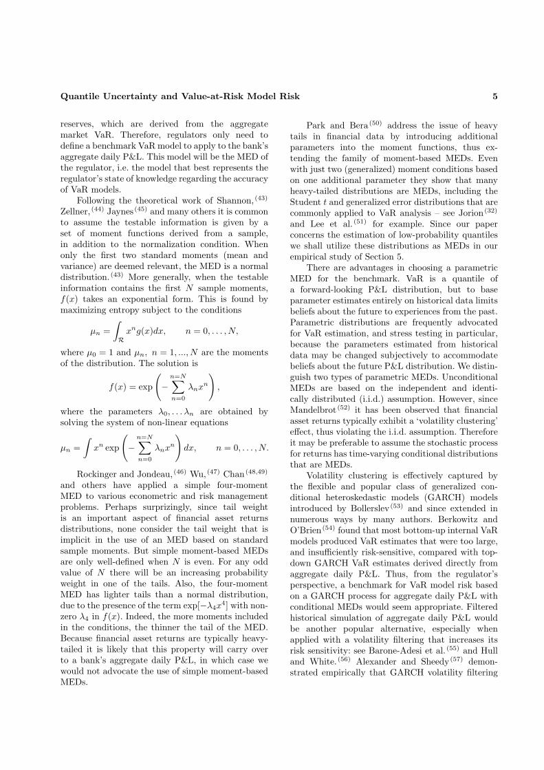
We estimate the two selected benchmark modelparameters using a ‘rolling window’ framework thatis standard practice for VaR estimation. Each samplecontains n consecutive observations on the bank’saggregate daily P&L, and a sample is rolled forwardone day at a time, each time re-estimating the modelparameters. Figure 3 compares the 1% quantile ofthe Student t distribution with the 1% quantile ofthe normal AGARCH process on the last day of eachrolling window. Also shown is the bank’s aggregateP&L for the day corresponding to the quantileestimate, between 3 September 2007 and 18 March2008. The effect of the banking crisis is evidenced bythe increase in volatility of daily P&L which beganwith the shock collapse of Lehmann Brothers in midSeptember 2008. Before this time the 1% quantilesof the unconditional Student t distribution werevery conservative predictors of daily losses, becausethe rolling windows included the commodity crisisof 2006. Yet at the time of the banking crisis theStudent t model clearly underestimated the lossesthat were being experienced. Even worse, from thebank’s point of view, the Student t model vastlyover-estimated the losses made during the aftermathof the crisis in early 2009 and would have led tocrippling levels of risk capital reserves. Even thoughwe used n = 200 for fitting the unconditional Studentt distribution and a much larger sample, with n =800, for fitting the normal AGARCH process it isclear that the GARCH process captures the strongvolatility clustering of daily P&L far better thanthe unconditional MED. True, the AGARCH processoften just misses a large unexpected loss, but becauseit has the flexibility to respond the very next day, theAGARCH process rapidly adapts to changing marketconditions just as a VaR model should.

In an extensive study of the aggregate P&Lof several large commercial banks, Berkowitz andO’Brien (54) found that GARCH models estimatedon aggregate P&L are far more accurate predictors ofaggregate losses than the bottom-up VaR figures thatmost banks use for regulatory capital calculations.Figure 3 verifies this finding by also depicting the1% daily VaR reported by the bank, multiplied by

−1 since it is losses rather than profits that VaR issupposed to cover. This time series has many featuresin common with the 1% quantiles derived from theStudent t distribution. The substantial losses of upto $80m per day during the last quarter of 2008were not predicted by the bank’s VaR estimates,yet following the banking crisis the bank’s VaR wasfar too conservative. We conclude, like Berkowitzand O’Brien, (54) that unconditional approaches aremuch less risk sensitive than GARCH models and forthis reason we choose the normal AGARCH ratherthan the Student t as our benchmark for model riskassessment below.

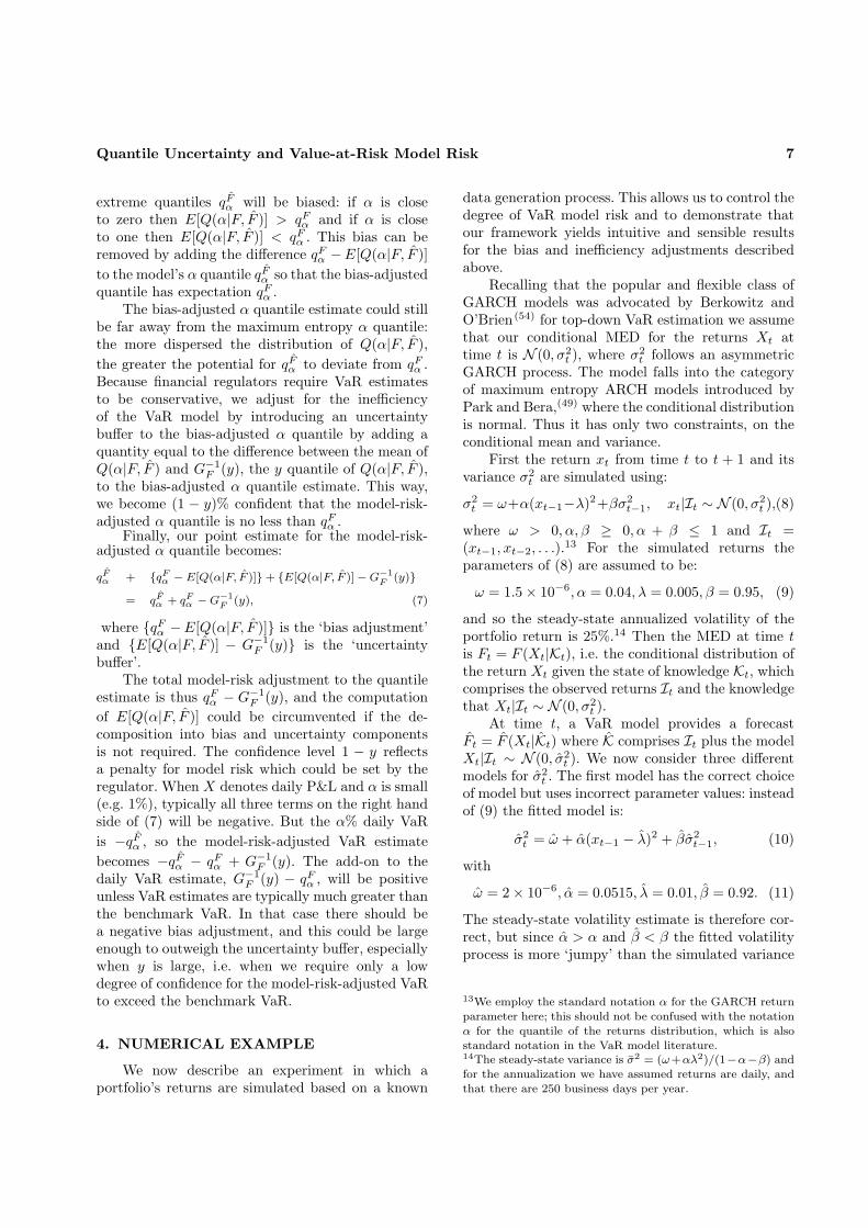
Figure 4 again depicts −1× the bank’s aggregatedaily VaR, denoted −VaRt in the formula below.Now our bias adjustment is computed daily usingan empirical model-risk-adjusted VaR distributionbased on the observations in each rolling window.Under the normal AGARCH benchmark, for asample starting at T and ending at T + n, the dailyP&L distribution at time t, with T ≤ t ≤ T + nis N(0, σ2

t ) where σt is the time-varying standarddeviation of the AGARCH model. Following (3)we set αt = Φ

(− σ−1t VaRt

)for each day in the

window and then we use the empirical distributionof αt for T ≤ t ≤ T + n to generate themodel-risk-adjusted VaR distribution (6). Then,following (7), the bias adjustment at T + n isthe difference between the mean of the model-risk-adjusted quantile distribution and the benchmarkVaR at T + n.

Since the bank’s aggregate VaR is very con-servative at the beginning of the period but notlarge enough during the crisis, in Figure 4 a positivebias reduces the VaR prior to the crisis but duringthe crisis a negative bias increases the VaR. Havingapplied the bias adjustment we then set y = 25% in(7) to derive the uncertainty buffer corresponding toa 75% confidence that the RaVaR will be no less thanthe BVaR. This is the difference between the meanand the 25%-quantile of the model-risk-adjustedVaR distribution. Adding this uncertainty buffer tothe bias-adjusted VaR we obtain the 75% RaVaRdepicted in Figure 4 which is given by (7). Thisis more variable than the bank’s original aggregateVaR, but risk capital is based on an average VaRfigure over the last 60 days (or the previous VaR, ifthis is greater) so the adjustment need not induceexcessive variation in risk capital, which would bedifficult to budget.

12 Alexander & Sarabia

Fig. 1. Density of quantile probabilities. Empirical distribu-tion of αt derived from (14) with α = 1%, based on 10,000daily returns simulated using (8) with parameters (9).

00.050.10.150.20.25

0% 1% 2% 3% 4% 5% 6%AGARCHEWMARegulatory

Fig. 2. Density of model-risk-adjusted daily VaR. Empiricaldensities of the model-risk-adjusted VaR estimates F−1(α)with α = 1%, based on the 10,000 observations on α whosedensity is shown in Figure 1.

00.050.10.150.20.250.30.35

2 2.5 3 3.5 4 4.5 5 5.5 6AGARCHEWMARegulatory

6. APPLICATION TO NON-FINANCIALPROBLEMS

Quantile-based risk assessment has become stan-dard practice in a wide variety of non-financialdisciplines, especially in environmental risk as-sessment and in statistical process control. Forinstance, applications to hydrology are studiedby Arsenault and Ashkar (62) and Chebana andOuarda, (63) and other environmental applicationsof quantile risk assessments include climate change(Katz et al., (64) and Diodato and Bellocchi, (65))wind power (66) and nuclear power (67). In statisticalprocess control, quantiles are used for computingcapability indices, (68) for measuring efficiency (69)

and for reliability analysis. (70)

In these contexts the uncertainty surroundingquantile-based risk assessments has been the subjectof many papers (36,71,72,73,74,75). Both model choice

and parameter uncertainty has been considered. Forinstance, Vermaat and Steerneman (76) discuss modi-fied quantiles based on extreme value distributions inreliability analysis, and Sveinsson et al. (77) examinethe errors induced by using a sample limited to asingle site in a regional frequency analysis.

As in banking, regulations can be a key driver forthe accurate assessment of environmental risks suchas radiation from nuclear power plants. Nevertheless,health or safety regulations are unlikely to extendas far as requirements for regular monitoring andreporting of quantile risks in the foreseeable future.The main concern about the uncertainty surroundingquantile risk assessment is more likely to come fromsenior management, in recognition that inaccuraterisk assessment could jeopardize the reputation ofthe firm, profits to shareholders and/or the safetyof the public. The question then arises: if it isa senior manager’s knowledge that specifies thebenchmark distribution for model risk assessment,why should this benchmark distribution not beutilized in practice?

As exemplified by the work of Sveinsson etal., (77) the time and expense of utilizing a completesample of data may not be feasible except on afew occasions where a more detailed risk analysisis performed, possibly by an external consultant.In this case the most significant source of modelrisk in regular risk assessments would stem fromparameter uncertainty. Model choice might also bea source of risk when realistic model assumptionswould lead to systems that are too costly andtime-consuming to employ on a daily basis. Forinstance, Merrik et al. (2005) point out that theuse of Bayesian simulation for modelling large andcomplex maritime risk systems should be consideredstate-of-the-art, rather than standard practice. Alsoin reliability modelling, individual risk assessmentsfor various components are typically aggregated toderive the total risk for the system. A full accountof component default codependencies may requirea lengthy scenario analyses based on a complexmodel (e.g. multivariate copulas with non-standardmarginal distributions). This type of risk assessmentmight not be feasible every day, but if it could beperformed on an occasional basis then it could beused as a benchmark for adjusting everyday quantileestimates for model risk.

Generalizations and extensions to higher dimen-sions of the benchmark model could be implemented.A multivariate parametric MED for the benchmarkmodel can be obtained using similar arguments to

Quantile Uncertainty and Value-at-Risk Model Risk 13

Fig. 3. Daily P&L, daily VaR and two potential benchmarkVaRs. The bank’s daily P&L is depicted by the grey lineand it’s ‘bottom-up’ daily VaR estimates by the black line.The dotted and dashed lines are the Student t (unconditionalMED) benchmark VaR and the normal AGARCH (conditionalMED) benchmark VaR.

-100

-80

-60

-40

-20

0

20

40

60

80

Daily P&L Student t Normal AGARCH Daily VaR

those used in the univariate case. In an engineeringcontext, Kapur (78) have considered several classesof multivariate MED. Zografos (79) characterizedPearson’s type II and VII multivariate distributions,Aulogiaris and Zografos (80) the symmetric Kotz andBurr multivariate families and Bhattacharya (81) theclass of multivariate Liouville distributions. Closedexpressions for entropies in several multivariatedistributions have been provided by Ahmed andGokhale (82) and Zografos and Nadarajah. (83)

A major difference between financial and non-financial risk assessment is the availability of data.For instance, in the example described in theprevious section the empirical distributions formodel-risk-adjusted quantiles were derived fromseveral years of regular output from the benchmarkmodel. Clearly, the ability to generate the adjustedquantile distribution from a parametric distributionfor α, such as the beta distribution (5), opensthe methodology to applications where relativelyfew observations on the benchmark quantile areavailable, but there are enough to estimate theparameters of a distribution for α.

7. SUMMARY

This paper concerns the model risk of quantile-based risk assessments, with a focus on the riskof producing inaccurate VaR estimates becauseof an inappropriate choice of VaR model and/orinaccuracy in the VaR model parameter estimates.We develop a statistical methodology that providesa practical solution to the problem of quantifying the

Fig. 4. Aggregate VaR, bias adjustment and 75% RaVaR.The bank’s daily VaR estimates are repeated (black line) andcompared with the bias-adjustment (grey line) and the finalmodel-risk-adjusted VaR at the 75% confidence level (dottedline) based on the normal AGARCH benchmark model.

-100

-80

-60

-40

-20

0

20

40

60

80

Daily VaR Bias 75% RaVaR

regulatory capital that should be set aside to coverthis type of model risk, under the July 2009 BaselII proposals. We argue that there is no better choiceof model risk benchmark than a maximum entropydistribution since, by definition, this embodies theentirety of information and beliefs, no more and noless. In the context of the model risk capital chargeunder the Basel II Accord the benchmark couldbe specified by the local regulator; more generallyit should be specified by any authority that isconcerned with model risk, such as the Chief RiskOfficer. Then VaR model risk is assessed using a top-down approach to compute the benchmark VaR fromthe bank’s total daily P&L, and comparing this withthe bank’s aggregate daily VaR, which is typicallyderived using a computationally intensive bottom-up approach that necessitates many approximationsand simplifications.

The main ideas are as follows: in the presenceof model risk an α quantile is at a different quantileof the benchmark model, and has an associated tailprobability under the benchmark that is stochastic.Thus, the model-risk-adjusted quantile becomesa generated random variable and its distributionquantifies the bias and uncertainty due to modelrisk. A significant bias arises if the aggregate VaRestimates tend to be consistently above or belowthe benchmark VaR, and this is reflected in asignificant difference between the mean of the model-risk-adjusted VaR distribution and the benchmarkVaR. Even when the bank’s VaR estimates havean insignificant bias, an adjustment for uncertaintyis required because the difference between thebank’s VaR and the benchmark VaR could vary

14 Alexander & Sarabia

considerably over time. The bias and uncertainty inthe VaR model, relative to the benchmark, determinea risk capital adjustment for model risk whose sizewill also depend on the confidence level regulatorsrequire for the adjusted risk capital to be no lessthan the risk capital based on the benchmark model.

Our framework was validated and illustrated bya numerical example which considers three commonVaR models in a simulation experiment where thedegree of model risk has been controlled. A furtherempirical example describes how the model-riskadjustment could be implemented in practice givenonly two time series, on the bank’s aggregate VaRand its aggregate daily P&L, which are in any casereported daily under banking regulations.

Further research would be useful on backtest-ing the model-risk-adjusted estimates relative tocommonly-used VaR models, such as the RiskMetricsmodels considered in this paper. Where VaR modelsare failing regulatory backtests and thus being heav-ily penalized or even disallowed, the top-down model-risk-adjustment advocated in this paper would bevery much more cost effective than implementinga new or substantially modified bottom-up VaRsystem.

There is potential for extending the methodologyto the quantile-based metrics that are commonlyused to assess non-financial risks in hydrology,climate change, statistical process control and reli-ability analysis. In the case that relatively few obser-vations on the model and benchmark quantiles areavailable, the approach should include a parameteri-zation the model-risk-adjusted quantile distribution,for instance as a beta-generated distribution.

ACKNOWLEDGMENTS

The authors would like to thank to the associateeditor and two anonymous reviewers for manyconstructive comments that improved the origi-nal version. The second author thanks Ministeriode Economıa y Competitividad, Spain (ECO2010-15455) for partial support.

REFERENCES

1. Basel Committee on Banking Supervision. Amendment tothe capital accord to incorporate market risks. Bank forInternational Settlements, Basel, 1996.

2. Basel Committee on Banking Supervision. Internationalconvergence of capital measurement and capital stan-

dards: A revised framework. Bank for InternationalSettlements, Basel, 2006.

3. Basel Committee on Banking Supervision. Revisions tothe Basel II market risk framework. Bank for InternationalSettlements, Basel, 2009.

4. Hendricks D. Evaluation of Value-at-Risk models usinghistorical data. FRBNY Economic Policy Review, 1996;April:39-69.

5. Perignon C, Smith D. The level and quality of Value-at-Risk disclosure by commercial banks. Journal of Bankingand Finance, 2010; 34(2):362-377.

6. Pritsker M. The hidden dangers of historical simulation.Journal of Banking and Finance, 2006; 30:561-582.

7. RiskMetrics. Technical Document. Available from theRiskMetrics website, 1997.

8. Hull J, White A. Value at risk when daily changes inmarket variables are not normally distributed. Journal ofDerivatives, 1998; 5(3):9-19.

9. Mittnik S, Paolella M. Conditional density and Value-at-Risk: prediction of Asian currency exchange rates. Journalof Forecasting, 2000; 19:313-333.

10. Venter J, de Jongh P. Risk estimation using the normalinverse Gaussian distribution. Journal of Risk, 2002; 4:1-23.

11. Angelidis T, Benos A, Degiannakis S. The use of GARCHmodels in VaR estimation. Statistical Methodology, 2004;1(2):105-128.

12. Hartz C, Mittnik S, Paolella M. Accurate Value-at-Riskforecasting based on the normal-GARCH model. Compu-tational Statistics and Data Analysis, 2006; 51(4):2295-2312.

13. Kuan C-M, Yeh J-H, Hsu Y-C. Assessing Value-at-Risk with CARE: the conditional autoregressive expectilemodels. Journal of Econometrics, 2009; 150(2):261-270.

14. Kupiec P. Techniques for verifying the accuracy ofrisk measurement models. Journal of Derivatives, 1995;3(2):73-84.

15. Christoffersen P. Evaluating interval forecasts. Interna-tional Economic Review, 1998; 39:841-862.

16. Berkowitz J, Christoffersen P, Pelletier D. EvaluatingVaR models with desk-level data. Management Science,Management Science, 2011; 57:2213-2227.

17. Engle R, Manganelli S. CAViaR: Conditional autoregres-sive Value at Risk by regression quantile. Journal ofBusiness and Economic Statistics, 2004; 22:367-381.

18. Turner L. The Turner review: A regulatory response tothe global banking crisis. Financial Services Authority,London, 2009.

19. Taleb N. The black swan: The impact of the highlyimprobable. Penguin, 2007.

20. Beder T. VAR: Seductive but dangerous. FinancialAnalysts Journal, 1995; 51(5):12-24.

21. Bernardo JM, Smith AFM. Bayesian Theory. Wiley,Chichester, UK, 1994.

22. O’Hagan A. Kendall’s Advanced Theory of Statistics. Vol2B: Bayesian Inference. Edward Arnold, London, 1994.

23. Modarres R, Nayak TK, Gastwirth JL. Estimation ofupper quantiles model and parameter uncertainty. Com-putational Statistics and Data Analysis, 2002; 39:529-554.

24. Giorgi G, Narduzzi C. Uncertainty of quantile estimatesin the measurement of self-similar processes. In: Interna-tional Workshop on Advanced Methods for UncertaintyEstimation Measurements, AMUEM 2008, Sardagna,Trento, Italy, 2008.

25. Figlewski S. Estimation error in the assessment offinancial risk exposure. SSRN-id424363, version of June29, 2003.

26. Derman E. Model risk. Risk, 1996; 9(5):139-145.27. Simons K. Model error - evaluation of various finance

Quantile Uncertainty and Value-at-Risk Model Risk 15

models. New England Economic Review, 1997; Nov-Dec:17-28.

28. Crouhy M, Galai D, Mark R. Model risk. Journal ofFinancial Engineering, 1998; 7:267-288.

29. Green T, Figlewski S. Market risk and model risk for afinancial institution writing options. Journal of Finance,1999; 54:1465-1499.

30. Kato T, Yoshiba T. Model risk and its control. Monetaryand Economic Studies, 2000; December:129-157.

31. Rebonato R. Managing Model Risk. In Volume 2 ofMastering Risk, C. Alexander (ed.), Pearson UK, 2001.

32. Jorion P. Measuring the risk in value at risk. FinancialAnalysts Journal, 1996; 52:47-56.

33. Talay D, Zheng Z. Worst case model risk management.Finance and Stochastics, 2002; 6:517-537.

34. Kerkhof J, Melenberg B, Schumacher H. Model risk andcapital reserves. Journal of Banking and Finance, 2010;34:267-279.

35. Reiss R, Thomas M. Statistical Analysis of Extreme Val-ues with Applications to Insurance, Finance, Hydrologyand Other Fields. Birkhauser Verlag, Basel, 1997.

36. Cairns A. A discussion of parameter and model un-certainty in insurance. Insurance: Mathematics andEconomics, 2000; 27:313-330.

37. Matthys G, Delafosse E, Guillou A, Beirlant J. Estimatingcatastrophic quantile levels for heavy-tailed distributions.Insurance: Mathematics and Economics, 2004; 34:517-537.

38. Dowd K, Blake D. After VaR: The theory, estimation andinsurance applications of quantile-based risk measures.Journal of Risk and Insurance, 2009; 73(2):193-229.

39. Cont R. Model uncertainty and its impact on the pricingof derivative instruments. Mathematical Finance, 2006;16(3):519-547.

40. Hull J, Suo W. A methodology for assessing model riskand its application to the implied volatility functionmodel. Journal of Financial and Quantitative Analysis,2002; 37(2):297-318.

41. Branger N, Schlag C. Model risk: A conceptual frameworkfor risk measurement and hedging. Working Paper, EFMABasel Meetings. Available from SSRN, 2004.

42. Ebrahimi N, Maasoumi E, Soofi E. Ordering univariatedistributions by entropy and variance. Journal of Econo-metrics, 1999; 90:317-336.

43. Shannon C. The mathematical theory of communication,Bell System Technical Journal July-Oct. Reprinted in:C.E. Shannon and W. Weaver, The Mathematical Theoryof Communication University of Illinois Press, 1948;Urbana, IL 3-91.

44. Zellner A. Maximal data information prior distributions.In: A. Aykac and C. Brumat, eds., New methods in theapplications of Bayesian methods. North-Holland, 1977.

45. Jaynes E. Papers on Probability, Statistics and StatisticalPhysics. Edited by R.D. Rosenkrantz, Reidel PublishingCompany, Dordrecht, 1983.

46. Rockinger M, Jondeau E. Entropy densities with anapplication to autoregressive conditional skewness andkurtosis. Journal of Econometrics, 2002; 106:119-142.

47. Wu X. Calculation of maximum entropy densities with ap-plication to income distribution. Journal of Econometrics,2003; 115(2):347-354

48. Chan F. Modelling time-varying higher moments withmaximum entropy density. Mathematics and Computersin Simulation, 2009; 79(9):2767-2778.

49. Chan F. Forecasting value-at-risk using maximum en-tropy. 18th World IMACS / MODSIM Congress, Cairns,Australia, 2009.

50. Park S, Bera A. Maximum entropy autoregressive condi-tional heteroskedasticity model. Journal of Econometrics,2009; 150(2):219-230.

51. Lee M-C, Su J-B, Liu H-C. Value-at-risk in US stock in-dices with skewed generalized error distribution. AppliedFinancial Economics Letters, 2008; 4(6):425-431.

52. Mandelbrot B. The variation of certain speculative prices.Journal of Business, 1963; 36:394-419.

53. Bollerslev T. A conditionally heteroskedastic time seriesmodel for speculative prices and rates of return. Reviewof Economics and Statistics, 1987; 69(3):542-547.

54. Berkowitz J, O’Brien J. How accurate are Value-at-Riskmodels at commercial banks? Journal of Finance, 2002;55:1093-1111.

55. Barone-Adesi G, Bourgoin F, Giannopoulos K. Don’t lookback. Risk, 1998; 11(8):100-103.

56. Hull J, White A. Incorporating volatility updatinginto the historical simulation method for Value-at-Risk.Journal of Risk, 1998; 1:5-19.

57. Alexander C, Sheedy E. Developing a stress testingframework based on market risk models. Journal ofBanking and Finance, 2008; 32(10):2220-2236.

58. Eugene N, Lee C, Famoye F. The beta normal distribu-tion and its applications. Communications in Statistics,Theory and Methods, 2002; 31:497-512.

59. Jones M. Families of distributions arising from distribu-tions of order statistics. Test, 2004; 13(1):1-43.

60. Zografos K, Balakrishnan, N. On families of beta- and gen-eralized gamma-generated distributions and associatedinference. Statistical Methodology, 2009; 6(4):344-362.

61. Nelson DB. Conditional heteroskedasticity in asset re-turns: A new approach. Econometrica, 1991; 59:347-370.

62. Arsenault M, Ashkar F. Regional flood quantile esti-mation under linear transformation of the data. WaterResources Research, 2000; 36(6):1605-1610.

63. Chebana F, Ouarda T. Multivariate quantiles in hydrolog-ical frequency analysis. Environmetrics, 2011; 22(1):63-78.

64. Katz R, Parlange M, Naveau P. Statistics of extremes inhydrology. Advances in Water Resources, 2002; 25:1287-1304.

65. Diodato N, Bellocchi G. Assessing and modelling changesin rainfall erosivity at different climate scales. EarthSurface Processes and Landforms, 2009; 34(7):969-980.

66. Bremnes J. Probabilistic wind power forecasts using localquantile regression. Wind Energy, 2004; 7(1):47-54.

67. Rumyantsev A. Safety prediction in nuclear power.Atomic Energy, 2007; 102(2):94-99.

68. Anghel C. Statistical process control methods from theviewpoint of industrial application. Economic QualityControl, 2001; 16(1):49-63.

69. Wheelock D, Wilson P. Non-parametric, unconditionalquantile estimation for efficiency analysis with an appli-cation to Federal Reserve check processing operations.Journal of Econometrics, 200; 145:209-225.

70. Unnikrishnan Nair N, Sankaran P. Quantile-based relia-bility analysis. Communications in Statistics - Theory andMethods, 2009; 38(2):222-232.

71. Mkhandi S, Kachroo R, Guo S. Uncertainty analysisof flood quantile estimates with reference to Tanzania.Journal of Hydrology, 1996; 185, 317-333.

72. Pinson P, Kariniotakis G. On-line assessment of predictionrisk for wind power production forecasts. Wind Energy,2004; 7(2):119-132.

73. Noon B, Cade B, Flather C. Quantile regression revealshidden bias and uncertainty in habitat models. Ecology,2009; 86(3):786-800.

74. Merrick J, Van Dorp R, Dinesh V. Assessing uncertaintyin simulation-based maritime risk assessment. Risk Anal-ysis, 2005; 25(3):731-743.

75. Peng L, Qi Y. Confidence regions for high quantiles ofa heavy tailed distribution. Annals of Statistics, 2006;34(4):1964-1986.

16 Alexander & Sarabia

76. Vermaat M, Does R, Steerneman A. A modified quantileestimator using extreme-value theory with applications.Economic Quality Control, 2005; 20(1):31-39.

77. Sveinsson O, Salas J, Boes D. Uncertainty of quan-tile estimators using the population index floodmethod. Water Resources Research, 2003; 39(8), 1206doi:10.1029/2002WR001594

78. Kapur JN. Maximum Entropy Models in Engineering.John Wiley, New York, 1989.

79. Zografos K. On maximum entropy characterization ofPearson’s type II and VII multivariate distributions.Journal of Multivariate Analysis, 1999; 71:67-75.

80. Aulogiaris G, Zografos K. A maximum entropy charac-terization of symmetric Kotz type and multivariate Burrdistributions. Test, 2004; 13:65-83.

81. Bhattacharya B. Maximum entropy characterizationsof the multivariate Liouville distributions. Journal ofMultivariate Analysis, 2006; 97:1272-1283.

82. Ahmed NA, Gokhale DV. Entropy expressions andtheir estimators for multivariate distributions. IEEETransactions on Information Theory, 1989; 35:688-692.

83. Zografos K, Nadarajah S. Expressions for Renyi and Shan-non entropies for multivariate distributions. Statistics andProbability Letters, 2005; 71:71-84.