quantile-based inflation risk models
TRANSCRIPT

Quantile-based Inflation Risk Models
Eric Ghysels 1 Leonardo Iania 2 Jonas Striaukas 2
1UNC 2UC Louvain
National Bank of Belgiums biennial conference
GIS Quantile-based Inflation Risk Models NBB 2018 10 1 / 23

Outline
1 Introduction
2 Modeling inflation quantilesQuantilesSummary of the analysisIn- and out-of-sample analysis
3 Inflation risk measuresInflation risk measures: definitionsThe reaction of short-term interest rates to inflation risk
4 Conclusions
GIS Quantile-based Inflation Risk Models NBB 2018 10 2 / 23

Motivation
”In assessing the path for the federalfunds rate [...] FOMC participants takeaccount of the range of possibleeconomic outcomes, the likelihood ofthose outcomes, and the potentialbenefits and costs should they occur.”
Source: Minutes of the Federal Open Market Committee.March 20-21, 2018
Figure: Fan chart of PCE Inflation
Note: Median projection and confidence interval based onhistorical forecast errors. Source: Minutes of the Federal OpenMarket Committee. March 20-21, 2018
GIS Quantile-based Inflation Risk Models NBB 2018 10 3 / 23

Motivation
”Because the fan charts are constructedto be symmetric around the medianprojections, they do not reflect anyasymmetries in the balance of risks thatparticipants may see in their economicprojections.”
Minutes of the Federal Open Market Committee. March
20-21, 2018
Figure: Risks to PCE inflation
Note: FOMC participants assessments of risks around theireconomic projections. Source: Minutes of the Federal OpenMarket Committee. March 20-21, 2018
GIS Quantile-based Inflation Risk Models NBB 2018 10 4 / 23

Motivation
Zarnowitz and Lambros (1987) propose uncertainty measure using theinter-quantile range of survey data
Kilian and Manganelli (2008) develop structural model in whichmonetary authorities can have non-quadratic valuation of inflationcosts
Kilian and Manganelli (2007) estimate several inflation risk measuresusing GARCH model
Andrade et al. (2015) use survey data to extract the expectedinflation asymmetry and document its impact on realized inflation andchanges in monetary policy
GIS Quantile-based Inflation Risk Models NBB 2018 10 5 / 23

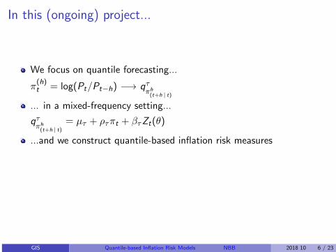
In this (ongoing) project...
We focus on quantile forecasting...
π(h)t = log(Pt/Pt−h) −→ qτ
πh(t+h | t)
... in a mixed-frequency setting...
qτπh
(t+h | t)
= µτ + ρτπt + βτZt(θ)
...and we construct quantile-based inflation risk measures
I I@Rτt|t−h = Inflation-at-riskI IQRτt|t−h = Interquantile rangeI ASYτt|t−h = Robust asymmetry
GIS Quantile-based Inflation Risk Models NBB 2018 10 6 / 23

In this (ongoing) project...
We focus on quantile forecasting...
π(h)t = log(Pt/Pt−h) −→ qτ
πh(t+h | t)
... in a mixed-frequency setting...
qτπh
(t+h | t)
= µτ + ρτπt + βτZt(θ)
...and we construct quantile-based inflation risk measuresI I@Rτt|t−h = Inflation-at-riskI IQRτt|t−h = Interquantile rangeI ASYτt|t−h = Robust asymmetry
GIS Quantile-based Inflation Risk Models NBB 2018 10 6 / 23

Outline
1 Introduction
2 Modeling inflation quantilesQuantilesSummary of the analysisIn- and out-of-sample analysis
3 Inflation risk measuresInflation risk measures: definitionsThe reaction of short-term interest rates to inflation risk
4 Conclusions
GIS Quantile-based Inflation Risk Models NBB 2018 10 7 / 23

Regression quantiles: intuition
Linear regression (Blue line)
E (rt |πt−1) = µ+ ρπt−1
Quantile regression (Red lines)
qτ (rt |πt−1) = µ(τ) + ρ(τ)πt−1
GIS Quantile-based Inflation Risk Models NBB 2018 10 8 / 23

Models
Quantile autoregressive model (QAR)
qτπh
(t+h | t)= µτ +
p−1∑j=0
ατ,jπt−j ≡ µτ + ρτπt +
q−1∑j=0
βτ,j∆πt−j
QAR distributed lag model with MIDAS component (QADL-MIDAS)
qτπh
(t+h | t)= µτ + ρτπt + βτZt(θ)
where
Zt(θτ ) =h∑
m=0
ωm(θτ )|∆πt−m|
GIS Quantile-based Inflation Risk Models NBB 2018 10 9 / 23

Modeling inflation quantiles: analysis
Setting
1 Based on monthly US CPI inflation (Headlines and CORE)
2 Period: 1960-01 to 2018-05
3 We focus on modeling/forecasting year-on-year inflation
4 Number of lags: 12.
Model comparison1 In-sample
I Are the regression coefficients quantile-dependent?I Is the MIDAS component informative about inflation quantiles?
2 Out-of-sampleI Which model forecast quantiles better?I At which horizon?
GIS Quantile-based Inflation Risk Models NBB 2018 10 10 / 23

In-sample analysisqπ
(h)t+h
(τ | Ft) = µτ + ρτπt +∑q−1
j=0 βτ,j∆πt−j
Quantile 0.05 0.25 0.5 0.75 0.95
µ -0.454 0.569 0.952 1.471 2.597(0.047) (0.000) (0.000) (0.000) (0.000)
ρ 0.502 0.593 0.713 0.866 1.101(0.000) (0.000) (0.000) (0.000) (0.000)
qπ
(h)t+h
(τ | Ft) = µτ + ρτπt + βτZt(θ)
Quantile 0.05 0.25 0.5 0.75 0.95
µ 0.062 0.723 0.581 0.658 1.891(0.371) (0.000) (0.000) (0.002) (0.000)
β -1.522 -0.446 2.738 3.507 2.335(0.014) (0.219) (0.000) (0.000) (0.014)
θ 43.668 35.510 1.124 1.716 1.000(0.112) (0.180) (0.465) (0.439) (0.482)
ρ 0.459 0.564 0.678 0.928 1.168(0.000) (0.000) (0.000) (0.000) (0.000)
GIS Quantile-based Inflation Risk Models NBB 2018 10 11 / 23
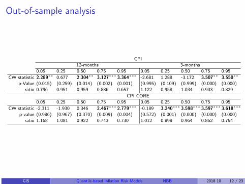
Out-of-sample analysis
CPI
12-months 3-months
0.05 0.25 0.50 0.75 0.95 0.05 0.25 0.50 0.75 0.95
CW statistic 2.289∗∗ 0.677 2.304∗∗ 3.127∗∗∗ 3.364∗∗∗ -2.681 1.288 -3.172 3.507∗∗ 3.550∗∗
p-Value (0.015) (0.259) (0.014) (0.002) (0.001) (0.995) (0.109) (0.999) (0.000) (0.000)
ratio 0.796 0.951 0.959 0.886 0.657 1.122 0.958 1.034 0.903 0.829
CPI CORE
0.05 0.25 0.50 0.75 0.95 0.05 0.25 0.50 0.75 0.95
CW statistic -2.311 -1.930 0.346 2.467∗∗∗ 2.779∗∗∗ -0.189 3.240∗∗∗ 3.598∗∗∗ 3.597∗∗∗ 3.618∗∗∗
p-value (0.986) (0.967) (0.370) (0.009) (0.004) (0.572) (0.001) (0.000) (0.000) (0.000)
ratio 1.168 1.081 0.922 0.743 0.730 1.012 0.898 0.964 0.862 0.754
GIS Quantile-based Inflation Risk Models NBB 2018 10 12 / 23

Outline
1 Introduction
2 Modeling inflation quantilesQuantilesSummary of the analysisIn- and out-of-sample analysis
3 Inflation risk measuresInflation risk measures: definitionsThe reaction of short-term interest rates to inflation risk
4 Conclusions
GIS Quantile-based Inflation Risk Models NBB 2018 10 13 / 23

Inflation risk measures (based on Andrade et al. (2015))
Inflation-at-risk
I@Rτ = q̂τ
Interquantile range
IQRτ = q̂1−τ − q̂τ
Contitional (robust) asymmetry
ASY τ =(q̂1−τ − q̂0.50)− (q̂0.50 − q̂τ )
IQRτ
GIS Quantile-based Inflation Risk Models NBB 2018 10 14 / 23

Conditional asymmetry comparison
QAR(12) conditional asymmetry
1970 1980 1990 2000 2010
-1
-0.5
0
0.5
1
QADL-MIDAS conditional asymmetry
1970 1980 1990 2000 2010
-1
-0.5
0
0.5
1
GIS Quantile-based Inflation Risk Models NBB 2018 10 15 / 23

Conditional asymmetry regimes
1970 1980 1990 2000 2010
-1
-0.5
0
0.5
1
Note: 12 months ahead conditional asymmetry (75%) for CPI data
GIS Quantile-based Inflation Risk Models NBB 2018 10 16 / 23

Inflation risk measures and monetary policy
We study the relationship between federal fund rates and inflation risk viaa two-step procedure:
1 Construct real-time risk measures
2 Regress federal fund rates changes on real-time risk measures and aset of control variables
GIS Quantile-based Inflation Risk Models NBB 2018 10 17 / 23

Step 2: Federal fund rates changes and real-time riskmeasures
Following Andrade, Ghysels, and Idier (2015), our augmented TaylorRule-type regression equation is:
∆it+1 = β0 + β1IQRτt|t−h + β2ASYτt|t−h + ρ′Ct + εt+1
where:
∆it+1 is the change in the effective federal funds rate (EFFR)
Ct containsI Lagged value of the EFFR, ∆itI Headline inflation, πh
tI Commodity inflation, πh
t,comI A measure of output gap compute using industrial production, ut .
GIS Quantile-based Inflation Risk Models NBB 2018 10 18 / 23

Table: Parameter estimates and model fit
01-Mar-1963 to 01-Apr-2018
IQR 5% ASY 5% IQR 25% ASY 25%
coeff. -0.014 0.192∗∗ -0.033 0.120∗∗
p-Value (0.403) (0.012) (0.237) (0.043)R2
adj 0.184 0.184
Dependent variable is real time change in effective federalfunds rate. ∗∗∗, ∗∗ and ∗ refer to 1, 5 and 10 percentsignificance levels.
∆it+1 = β0 + β1IQRτt|t−h + β2ASYτt|t−h + ρ′Ct + εt+1
GIS Quantile-based Inflation Risk Models NBB 2018 10 19 / 23

Table: Parameter estimates and model fit
01-Jan-1980 to 01-Apr-2018
IQR 5% ASY 5% IQR 25% ASY 25%
coeff. 0.004 0.108∗ 0.001 0.072p-Value (0.860) (0.068) (0.987) (0.190)
R2adj 0.179 0.179
01-Mar-1963 to 01-Dec-1978
IQR 5% ASY 5% IQR 25% ASY 25%coeff. -0.054∗∗∗ 0.297∗∗ -0.101∗∗∗ 0.106∗∗
p-Value (0.002) (0.022) (0.003) (0.059)R2
adj 0.364 0.383
01-Mar-1963 to 01-Nov-2008
IQR 5% ASY 5% IQR 25% ASY 25%coeff. -0.007 0.279∗∗ -0.035 0.136
p-Value (0.730) (0.050) (0.262) (0.126)R2
adj 0.190 0.189
GIS Quantile-based Inflation Risk Models NBB 2018 10 20 / 23

Outline
1 Introduction
2 Modeling inflation quantilesQuantilesSummary of the analysisIn- and out-of-sample analysis
3 Inflation risk measuresInflation risk measures: definitionsThe reaction of short-term interest rates to inflation risk
4 Conclusions
GIS Quantile-based Inflation Risk Models NBB 2018 10 21 / 23

Summary of results
1 We propose a new approach to extract quantile-based inflation riskmeasures
2 Our model accounts for absolute past inflation changes in quantilemodeling and can handle mixed-frequency data sampling
3 Our model performs favorably with respect to a standard QAR modelin terms of prediction of conditional quantiles
4 We use our model-based quantiles to construct inflation-risk measures
5 We show that there is a positive and significant relationship ofchanges in Effective Federal Funds rate and conditional asymmetry
6 Results are in line with survey data based inflation conditionalasymmetry, Andrade et al. (2015)
GIS Quantile-based Inflation Risk Models NBB 2018 10 22 / 23

References I
Andrade, P., E. Ghysels, and J. Idier (2015): “Tails of InflationForecasts and Tales of Monetary Policy,” .
Kilian, L. and S. Manganelli (2007): “Quantifying the risk ofdeflation,” Journal of Money, Credit and Banking, 39, 561–590.
——— (2008): “The central banker as a risk manager: Estimating theFederal Reserve’s preferences under Greenspan,” Journal of Money,Credit and Banking, 40, 1103–1129.
Zarnowitz, V. and L. A. Lambros (1987): “Consensus anduncertainty in economic prediction,” Journal of Political economy, 95,591–621.
GIS Quantile-based Inflation Risk Models NBB 2018 10 23 / 23