Department of Quantitative Social Science

Using M-quantile models as an alternativeto random effects to model the contextualvalue-added of schools in London

Nikos TzavidisJames J Brown

DoQSS Working Paper No. 10-11June 2010

DISCLAIMER

Any opinions expressed here are those of the author(s) and notthose of the Institute of Education. Research published in thisseries may include views on policy, but the institute itself takes noinstitutional policy positions.

DoQSS Workings Papers often represent preliminary work andare circulated to encourage discussion. Citation of such a papershould account for its provisional character. A revised version maybe available directly from the author.

Department of Quantitative Social Science. Institute ofEducation, University of London. 20 Bedford way, LondonWC1H 0AL, UK.

Using M-quantile models as an alternative to

random effects to model the contextualvalue-added of schools in LondonDr Nikos Tzavidis∗, James J Brown†‡

Abstract. The measurement of school performance for secondary schoolsin England has developed from simple measures of marginal performance atage 16 to more complex contextual value-added measures that account forpupil prior attainment and background. These models have been developedwithin the multilevel modelling environment (pupils within schools) but inthis paper we propose an alternative using a more robust approach based onM-quantile modelling of individual pupil efficiency. These efficiency measurescondition on a pupils ability and background, as do the current contextualvalue-added models, but as they are measured at the pupil level a varietyof performance measures can be readily produced at the school and higher(local authority) levels. Standard errors for the performance measures areprovided via a bootstrap approach, which is validated using a model-basedsimulation.

JEL classification: C14, C21, I21.

Keywords: School Performance, Contextual Value-Added, M-Quantile Mod-els, Pupil Efficiency, London.

∗University of Manchester. E-mail: (nikos.tzavidis@manchester.ac.uk)†Department of Quantitative Social Science, Institute of Education, University of London.20 Bedford Way, WC1H 0AL. E-mail: (j.brown@ioe.ac.uk)‡Acknowledgements. This research was undertaken as part of ADMIN at the Institute ofEducation, which is funded by the ESRC under their NCRM Methods Node programme(ref: RES-576-25-0014).

1. Introduction

The development of school performance measurement in England has seen a move from

specialist studies by academic institutions (for example Tymms and Coe, 2003 review the work

of the CEM Centre based at the University of Durham while Goldsten et al, 1993 is one example

analysing a well-known dataset on Inner London schools) through to the initial use of simple

school measures in national tables and the introduction of ‘value-added’ and the current

‘contextual value-added’ tables produced by DCFS (Ray, 2006). This current approach utilises

multilevel modelling (Goldstein, 2003) to allow for the control of individual pupil characteristics

such as prior attainment as well as more contextual factors such as the composition of pupil

performance within the school, leaving the school ‘random effect’ (with a confidence interval) as

a measure of the impact the school had on the pupil’s performance that cannot be explained by

measured characteristics of the pupil or their peers. These measures can be appropriate for

judging school performance but as Leckie and Goldstein (2009) show, not school choice by

parents, who need a measure of the school’s performance several years into the future. In this

paper we will concentrate on developing a measure of school performance appropriate for

judging current performance and therefore school accountability but not appropriate for school

choice. In addition, we will not impose apriori any structure on the data allowing the potential to

compare performance of Local Authorities without the need to include explicit additional

structure into our modelling. We apply the approach to evaluating schools in London using the

linked National Pupil Database (NPD) / Pupil Level Annual School Census (PLASC) data set

for the cohort of pupils in year 11 (age 16) in 2007/8. We produce appropriate measures of error

to accompany our school performance measures as well as map the performance across Local

Authorities showing that controlling for pupil characteristics goes some way to explaining

differing performance at age 16 for pupils across London.

2. Approaches to Measuring School Performance

The recent paper by Leckie and Goldstein (2009) gives an excellent history of the development

of school performance measurement in England resulting in the current contextual value-added

models outlined in Ray (2006). In this section we review this approach and highlight some

weaknesses. We propose an alternative approach that addresses some of the concerns expressed

in relation to the current approach.

5

2.1. Reviewing the Current Approach

The current approach outlined in Ray (2006), and more flexible extensions by Leckie (2009) and

Leckie and Goldstein (2009), essentially fits a linear model to the mean performance of pupils at

age 16 corresponding to the end of compulsory schooling (referred to as key-stage 4),

conditional on their prior attainment at age 11 (referred to as key-stage 2), the prior attainment

of other pupils in the same cohort within their school, and other contextual factors such as

whether the pupil receives free school meals (a means tested benefit associated with low income

families) and the deprivation of the local area the pupil lives in. The pupil performance is

measured by a score calculated from converting the grades in their eight best exams (typically

GCSEs) to a points score. The exams are taken at around age 16 at the end of compulsory

schooling in England. Often the performance measures are standardised, both at outcome and

prior attainment, to be mean zero and standard deviation one to aid the interpretation of impacts

but this is not necessarily required. The current CVA model (Ray, 2006) fits on the original scale

of the variables while the recent work by Leckie and Goldstein (2009) transform the data onto a

normal scale using the ranks of the original distributions. If the school has no additional impact

on performance, coming say from the management structure within the school and its support

of the teaching staff and pupil learning, the pupil residuals would be uncorrelated with each

other. In reality, there is a residual school effect evidenced by a non-zero correlation across pupil

residuals within schools (the mean of the pupil residuals is not zero) and therefore we can

efficiently model the structure using a multilevel regression approach (Goldstein, 2003). The

multilevel framework can then be extended considerably to allow for school effects over time

(Leckie and Goldstein, 2009 is a recent paper covering this), cross-classified models to allow for

the impact of local area (Leckie, 2009 going back to Garner and Raudenbush, 1991) as well as

mobility (Leckie, 2009, and Goldstein, Burgess and McConnell, 2007).

The approach in the current models used by DCSF (Ray, 2006) applies the simple random

effects specification giving a single measure of the school impact. The model assumes that this

school impact is additive and constant across the pupils within a school. The impact comes from

the school level residual in the random intercepts model and this is typically assumed to be

normally distributed with independence between schools, independence of pupils within schools

after controlling for the common school effect, and of course independence between the school

6

residuals and the pupil level variables in the model. This final assumption results in the constant

additive effect of the school. In reality, the assumptions of a normal distribution, constant effect,

and even independence between schools can be problematic.

The problems partly come from the outcome being modelled. The score only takes the best eight

GCSEs for each pupil to prevent a school entering pupils into lots of exams to inflate their

overall score (Ray, 2006). However, the performance of the best performing pupils is essentially

capped meaning that schools with higher performing pupils do not appear to add much value as

a linear model can extrapolate that these pupils should do better than the capped score allows.

Therefore the pupil residuals are lower and potentially forced to be negative leading to a low

estimate of the school impact. In other words, the capping violates the constant variance

assumptions of the model. We can deal with this within a multilevel framework by extending the

level one error structure to capture non-constant variance (Goldstein, 2003) but this is an

extension that has not been widely used. Goldstein and Thomas (1996) allow the pupil residual

variance to vary by gender while Goldstein et al (1993) explored variation on pupil prior

attainment. However, to the knowledge of the authors this approach has not been applied to the

more recent nationally available pupil performance data and it is not the approach we take here

to deal with this issue.

A related issue is the assumption of a uniform additive effect for the school across all pupils.

This can be violated two ways. Firstly, as outlined in the previous paragraph, the non-constant

variance and capping implies that adding the same absolute value to a pupil’s performance does

not have the same ‘value’ across the prior attainment range. It is easier to make absolute

improvements at the bottom end of the scale. Secondly, even if this first issue is not a problem,

the value added by the school may well depend on the pupil’s characteristics. The second point

can be incorporated by the use of random slopes at the school level (Goldstein and Thomas,

1996 is one example) and such adjustments are particularly relevant when parents are choosing a

suitable school (Leckie and Goldstein, 2009). However, in this paper we are restricting to the use

of school effects to judge current performance and therefore the single random intercept gives

an average of the school’s added value, even if it does not reflect the variable nature of that

impact for the different pupils within the school.

7

2.2. An Alternative Framework for Pupil Performance and School Effects

In Section 2.1 we have highlighted some of the issues that occur with the current application of

multilevel modelling. In this section we motivate an alternative approach that helps address some

of these issues. We start by considering the individual performance of the pupils. Each pupil has

a set of characteristics and context that drives their performance in the exams at age 16. If we

compare across pupils with similar backgrounds we can start to consider their relative

performance. This can be thought of as how efficient a pupil is with the particular set of

circumstances they have and leads us to explore the literature in relation to production efficiency.

More efficient pupils will perform better relative to those with similar inputs as measured by the

prior attainment and similar ‘production environment’ measured by the contextual covariates.

(Haveman and Wolfe, 1995 is an example from an Economic perspective viewing a child’s

achievement as the outcome of inputs by the pupil, their family and society or government.)

Kokic et al (1997) introduce the use of m-quantile regression as a measurement of relative

production-performance that they argue has good properties and we propose applying this

technique to model the pupils’ efficiency.

Once we have an efficiency measure for each pupil, we then impose the school structure. If the

school has an impact it will allow pupils to be more efficient (inefficient) and so the average

efficiency within a school will move away from the average efficiency across all pupils (around

0.5). This is similar to looking for correlation within schools in the pupil level errors. This

aggregating of the individual quantile measures to get an ‘area’ summary links in with the recent

extension of m-quantile models to small area estimation problems, where we wish to account for

small area effects in our modelling (Chambers and Tzavidis, 2006). Interestingly, this school

measure will then give a summary to aid judging the school performance but it will no longer

necessarily satisfy the fourth criterion for measuring production-performance laid down by

Kokic et al (1997). This is because the school impact for a group of pupils within the school can

depend on the prior attainment and links to the concept of random slopes for schools in the

multilevel literature.

This alternative approach still forces the idea of a constant school effect but this effect is no

longer a simple additive impact across pupils. It actually represents an efficiency gain or loss

relative to the population average of the pupils. The actual impact on a student’s performance as

measured by their exam scores will depend on the distribution of performance at their level of

8

the covariates and this therefore allows for the differing variance in performance across the

range of prior attainment. Related to this we also reduce the potential impact of capping as the

approach recognises that at high levels of prior attainment the distribution of the outcome will

be much tighter as a result of the capping but there will still be an ordering from the most to

least efficient pupils.

As this approach is based on m-quantiles it is naturally more robust to distributional issues with

the outcome variable than a standard multilevel approach. An alternative approach taken by

Leckie and Goldstein (2009) to address this issue is via a transformation of the data to make it

better approximate a normal distribution. We prefer to try a modelling approach that is robust

rather than a transformation approach. In addition, the transformation approach does not tackle

the issue of the non-constant residual variance and this requires more complex random

structures, such as a random slope at level one on prior attainment, increasing further the

complexity of the model.

An additional advantage of this approach is that we get the full distribution of the pupil

efficiencies within schools but this is driven by the data rather than a distributional assumption

imposed apriori on the pupil level residuals. Therefore we can summarize the school effect as

not only the mean but other summaries such as the median or the proportion of pupils within a

school above the upper quartile. Also, as we have not imposed structure on the model so we can

summarize pupil performance at the local authority level (the local administrative units within

London) or compare the performance of groups within school. In the subsequent analysis we

will demonstrate these aspects by mapping performance at the local authority level across

London and comparing the performance within mixed schools for males and females. Of course,

the multilevel framework can also provide a measure at the local authority level by extending to

three levels and a school level random slope on gender (Goldstein and Thomas, 1996) would

allow for a difference in the school impact by gender. However, we see the advantage of our

approach being you model the pupil level performance and can then explore performance at

different levels (schools, local geography, sub-groups) without having to pre-specify them in the

model.

9

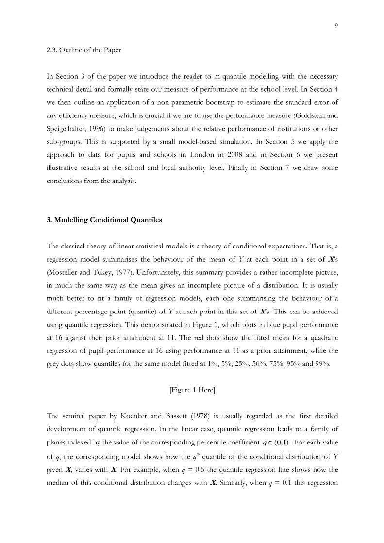
2.3. Outline of the Paper

In Section 3 of the paper we introduce the reader to m-quantile modelling with the necessary

technical detail and formally state our measure of performance at the school level. In Section 4

we then outline an application of a non-parametric bootstrap to estimate the standard error of

any efficiency measure, which is crucial if we are to use the performance measure (Goldstein and

Speigelhalter, 1996) to make judgements about the relative performance of institutions or other

sub-groups. This is supported by a small model-based simulation. In Section 5 we apply the

approach to data for pupils and schools in London in 2008 and in Section 6 we present

illustrative results at the school and local authority level. Finally in Section 7 we draw some

conclusions from the analysis.

3. Modelling Conditional Quantiles

The classical theory of linear statistical models is a theory of conditional expectations. That is, a

regression model summarises the behaviour of the mean of Y at each point in a set of X’s

(Mosteller and Tukey, 1977). Unfortunately, this summary provides a rather incomplete picture,

in much the same way as the mean gives an incomplete picture of a distribution. It is usually

much better to fit a family of regression models, each one summarising the behaviour of a

different percentage point (quantile) of Y at each point in this set of X’s. This can be achieved

using quantile regression. This demonstrated in Figure 1, which plots in blue pupil performance

at 16 against their prior attainment at 11. The red dots show the fitted mean for a quadratic

regression of pupil performance at 16 using performance at 11 as a prior attainment, while the

grey dots show quantiles for the same model fitted at 1%, 5%, 25%, 50%, 75%, 95% and 99%.

[Figure 1 Here]

The seminal paper by Koenker and Bassett (1978) is usually regarded as the first detailed

development of quantile regression. In the linear case, quantile regression leads to a family of

planes indexed by the value of the corresponding percentile coefficient (0,1)q ∈ . For each value

of q, the corresponding model shows how the qth quantile of the conditional distribution of Y

given X, varies with X. For example, when q = 0.5 the quantile regression line shows how the

median of this conditional distribution changes with X. Similarly, when q = 0.1 this regression

10

line separates the top 90% of the conditional distribution from the lower 10%. A linear model

for the qth conditional quantile of Y given a vector of covariates X is

( | ) = T

q qQ Y ββββX X , (1)

and qββββ is estimated by minimising ( ) ( ){ }

1

(1 ) 0 0=

− − − ≤ + − >∑n

T T T

i i i i i i

i

y q I y qI yx x xβ β ββ β ββ β ββ β β with

respect to ββββ . Solutions to this minimisation problem are usually obtained using linear

programming methods (Koenker and D’Orey, 1987). Functions for fitting quantile regression

now exist in standard statistical software, e.g. the. R statistical package (R Development Core

Team, 2004).

3.1. Using the M-quantile approach

Quantile regression can be viewed as a generalisation of median regression. In the same way,

expectile regression (Newey and Powell, 1987) is a “quantile-like” generalisation of mean

regression. M-quantile regression (Breckling and Chambers, 1988) integrates these concepts

within a common framework defined by a “quantile-like” generalisation of regression based on

influence functions (M-regression).

The M-quantile of order q for the conditional density of Y given X is defined as the solution

( ; )ψq

Q X of the estimating equation ( ) ( | ) 0ψ − =∫ qY Q f Y dYX , where ψ denotes the

influence function associated with the M-quantile. A linear M-quantile regression model is one

where we assume that

( | ; ) ( )ψψ = T

qQ Y qββββX X , (2)

that is, we allow a different set of regression parameters for each value of q. For specified q and

ψ , estimates of these regression parameters can be obtained by solving the estimating equations

1

( )ψψ=

=∑n

q iq i

i

r 0X , (3)

where ( )ψ ψ= − T

iq i ir Y qββββX , { }1( ) 2 ( ) ( 0) (1 ) ( 0)

q iq iq iq iqr s r qI r q I rψ ψ ψ ψψ ψ −= > + − ≤ and s is a

suitable robust estimate of scale, e.g. the MAD estimate / 0.6745iq

s median r ψ= . In this paper

we use a Huber Proposal 2 influence function, ( ) ( ) sgn( )u uI c u c c uψ = − ≤ ≤ + . Provided c is

11

bounded away from zero, estimates of ( )ψ qββββ are obtained by iterative weighted least squares.

The steps of the algorithm are as follows:

1. Start with initial estimates ( )ψ qββββ and s;

2. Form residuals iqr ψ

3. Define weights ( ) /i q iq iq

w r rψ ψψ=

4. Update ( )ψ qββββ using weighted least squares regression with weights i

w ;

5. Iterate until convergence.

These steps can be implemented in R by a straightforward modification of the IWLS algorithm

used for fitting M-regression (Venables and Ripley, 2002, section 8.3).

M-quantile regression is synonymous to outlier robust estimation. However, an advantage of M-

quantile regression is that it allows for more flexibility in modelling. For example, the tuning

constant c can be used to trade robustness for efficiency in the M-quantile regression fit, with

increasing robustness/decreasing efficiency as we move towards quantile regression and

decreasing robustness/increasing efficiency as we move towards expectile regression.

3.2. An M-quantile measure of school performance

Let us assume that the output of a school j can be measured by a single variable Y for example,

GCSE performance and that this output is associated with a set of explanatory (input) variables

X and for the time being, let us assume that we have data only at school level. Kokic et al. (1997)

proposed a measure of production performance that is based on the use of M-quantile models.

Let us assume that the quantiles of the conditional distribution ( )|f Y X can be model using a

linear function as in (2).

Using (2), the M-quantile measure of performance is defined as follows: If the qth M-quantile

surface implied by (2) passes through ( )j j,Y X , the performance measure for the jth school is

j=p q and the higher the value of j

p the better the school performance. Until this point we have

assumed that data are available only at school level. In most cases, however, data are available for

12

pupils clustered with schools. This creates a two level hierarchical structure, which we should

account for. Below we use ij

Y and ij X to denote the data for pupil i in school j.

Multilevel models assume that variability associated with the conditional distribution of Y given

X can be at least partially explained by a pre-specified hierarchical structure. The idea of

measuring hierarchical effects via an M-quantile model has recently attracted a lot of interest in

the small area estimation literature (Chambers and Tzavidis 2006; Tzavidis et al. 2010) and also

in other applications (Yu and Vinciotti). Following the development in Chambers and Tzavidis

(2006), we characterise the conditional variability across the population of interest by the M-

quantile coefficients of the population units. For unit i in cluster (school) j with values ijY and

ijX , this coefficient is the value ij

p such that ( ; )ψ =ijp ij ij

Q YX . Note that these M-quantile

coefficients are determined at the population level. If a hierarchical structure does explain part of

the variability in the population data, we expect units within the clusters defined by this hierarchy

to have similar M-quantile coefficients. Consequently, we characterise a cluster by the location of

the distribution of its associated unit (pupil)-level M-quantile coefficients. In particular, the M-

quantile measure of performance is defined as

1

1

−

=

= ∑jN

j j ij

i

p N q . (4)

The measure of performance defined by (4) is an extension of the M-quantile measure of

performance proposed by Kokic et al. (1997) that accounts for the hierarchical structure of the

data. Estimation of (4) is performed as follows. Following Chambers and Tzavidis (2006), we

first estimate the M-quantile coefficients { }; ∈i

q i s of the sampled units without reference to the

groups (schools) of interest. A grid-based procedure for doing this under (3) is described by

Chambers and Tzavidis (2006) and can be used directly with (4). We first define a fine grid of q

values in the interval (0,1). Chambers and Tzavidis (2006) use a grid that ranges between (0.01 to

0.99) with step 0.01. We employ the same grid definition and then use the sample data to fit (3)

for each distinct value of q on this grid. The M-quantile coefficient for unit i with values i

Y and

iX is calculated by using linear interpolation over this grid to find the unique value

iq such that

ˆ ( ; )ψ ≈iq i i

Q YX . A school j specific M-quantile measure of performance, ˆj

p is then estimated

by the average value of the unit (pupil) M-quantile coefficients in school j ,

13

1

1

ˆ ˆ−

=

= ∑jn

j j ij

i

p n q . (5)

The advantage of this approach is that we have the efficiencies, i

q , for each pupil i and therefore

the averaging done in (5) to give the school value can be done also across a higher level of

geography (such as local authority) or done across pupil sub-groups such as males and females

within schools without the need to pre-specify complex structures in the modelling.

4. Mean Squared Error Estimation

In this section we describe a non-parametric bootstrap approach to MSE estimation of the M-

quantile measure of school performance that is based on the approach of Lombardia et al. (2003)

and Tzavidis et al. (2010). In particular, we define two bootstrap schemes that resample residuals

from an M-quantile model fit. The first scheme draws samples from the empirical distribution of

suitably re-centred residuals. The second scheme draws samples from a smoothed version of this

empirical distribution. Using these two schemes, we generate a bootstrap population, from which

we then draw bootstrap samples.

4.1. Implementing the Bootstrap

In order to define the bootstrap population, we first calculate the M-quantile model residuals

ˆ ( )ψ= −ij ij ij

e y qxT ββββ . A bootstrap finite population * *

{ , }, , 1, ,= ∈ = Kij ij

U y i U j dx with

* *ˆ ( )ψ= +ij ij ij

y q exT ββββ is then generated, where the bootstrap residuals *

ije are obtained by sampling

from an estimator of the CDF ˆ ( )G u of the ije . In order to define ˆ ( )G u , we consider two

approaches: (i) sampling from the empirical CDF of the residuals ije and (ii) sampling from a

smoothed CDF of these residuals. In each case, sampling of the residuals can be done in two

ways: (i) by sampling from the distribution of all residuals without conditioning on the group

(the unconditional approach); and (ii) by sampling from the conditional distribution of residuals

within the group j (the conditional approach). The empirical CDF of the residuals is

1

1

ˆ ( ) ( )−

= ∈

= − ≤∑∑j

d

ij s

j i s

G u n I e e u , (6)

14

where s

e is the sample mean of the ije . Similarly, the empirical CDF of these residuals in group j

is

1ˆ ( ) ( ),j

j j ij sj

i s

G u n I e e u−

∈

= − ≤∑ (7)

where sje is the sample mean of the ij

e in group j. A smoothed estimator of the unconditional

CDF is

( ){ }1 1

1

ˆ ( ) − −

= ∈

= − +∑∑j

d

ij s

j i s

G u n K h u e e , (8)

where h > 0 is a smoothing parameter and K is the CDF corresponding to a bounded symmetric

kernel density k. Similarly a smoothed estimator of the conditional CDF in group j is

( ){ }1 1ˆ ( ) − −

∈

= − +∑j

j j j ij sj

i s

G u n K h u e e , (9)

where 0>j

h and K are the same as above. In the empirical studies reported in Section 4.2, we

define K in terms of the Epanechnikov kernel, ( )( ) ( )2( ) 3 / 4 1 1= − <k u u I u , while the

smoothing parameters h and jh are chosen so that they minimize the cross-validation criterion

suggested by Bowman et al. (1998). That is, in the unconditional case, h is chosen in order to

minimize

{ }2

1

1

( ) ( ) ( )−

−= ∈

= − ≤ − ∑∑∫j

d

ij s i

j i s

CV h n I e e u G u du , (10)

where ( )−iG u is the version of ( )G u that omits sample unit i, with the extension to the

conditional case being obvious. It can be shown (Li and Racine, 2007, section 1.5) that choosing

h and jh in this way is asymptotically equivalent to using the MSE optimal values of these

parameters.

In what follows we denote by jp the unknown true M-quantile measure of school performance,

by ˆj

p the estimator of jp based on sample j

s , by *

jp the known true M-quantile measure of

school performance of the bootstrap population *

jU , and by ˆ ∗

jp the estimator of *

jp based on

bootstrap sample *

js .

We estimate the MSE of the M-quantile measure of school performance as follows. Starting

from the sample s, we generate B bootstrap populations, *bU , using one of the four above-

15

mentioned methods for estimating the CDF of the residuals. From each bootstrap population,

*bU , we select L samples using simple random sampling without replacement within the schools

with * =j j

n n . The bootstrap estimator of the MSE of ˆj

p is then

{ } ( )2

21 1 1 1 *

1 1 1 1

ˆ ˆ ˆ( )avB L B L

*bl *bl *bl b

j j j j j

b

L

l b l

MSE B L p p B L p p∧

− − − −

= = = =

= − + −

∑∑ ∑∑ . (11)

In (12) *b

jp is the school j value of the characteristic of interest for the bth bootstrap population

and 1

1

)v ˆ ˆ(a −

=

= ∑L

*bl *bl

j j

l

Lp L p , where ˆ*bl

jp is the estimator of this characteristic computed from the

lth sample of the bth bootstrap population, (b = 1,…,B, l = 1,…,L). Note that this bootstrap

procedure can also be used to construct confidence intervals for the value of jp by ‘reading off’

appropriate quantiles of the bootstrap distribution of ˆj

p .

4.2. Monte-Carlo evaluation of the MSE estimator

A small scale model-based Monte-Carlo simulation study was designed for evaluating the

performance of the bootstrap MSE estimator of the M-quantile measure of performance. The

population data on which this simulation was based is generated from a 2-level random

intercepts model (individuals nested within groups (schools)). The model parameters used for

generating the Monte-Carlo populations are obtained from fitting a 2-level random intercepts

model to the 2008 linked NPD / PLASC data. The outcome variable is the post attainment, we

control for the effect of prior attainment and the random effects are specified at the school level.

In particular, population data are generated using 57 14ij ij j ij

y x γ ε= − + + + , where

~ (27,4)ij

x N , ~ (0,17.15)j

Nγ and ~ (0,65.13)ij

Nε . We generate in total 250 populations

with a total size 16020 units in 40 schools. The school population sizes range from 200 to 590

with an average of 400 units per school. From each of the 250 populations we take independent

samples by randomly selecting pupils within the 40 schools. The group sample sizes range from

20 to 59 with an average of 40 units per group. For each sample, estimates of the M-quantile

16

measure of performance were obtained using the methodology of Section 3 and an M-quantile

model that included as main effect ijx . For each Monte-Carlo simulation bootstrap MSE

estimation for the M-quantile measure of performance was implemented by generating a single

bootstrap population and then taking L = 250 bootstrap samples from this population. The

bootstrap population was generated unconditionally, with bootstrap population values obtained

by sampling from the smoothed residual distribution generated by the sample data obtained in

each Monte Carlo simulation. The performance of the MSE estimator is assessed using the

percentage relative bias of the bootstrap MSE estimator defined by

( )1 1

1

ˆ( ) 100K

i ik ii

k

RB M mean M K M M− −

=

= − ×

∑ . (12)

Here the subscript i indexes the schools and the subscript k indexes the K Monte Carlo

simulations, with ˆik

M denoting the simulation k value of the MSE estimator in school i, and i

M

denotes the actual (i.e. Monte Carlo) MSE in area i. In addition to the relative bias we compute

coverage rates of 95% confidence intervals which are constructed using the M-quantile measure

of school performance plus or minus twice its estimated standard error. The coverage rate is

defined as the number of times this confidence interval includes the true M-quantile measure of

performance and for a 95% confidence interval this rate must be close to 95%.

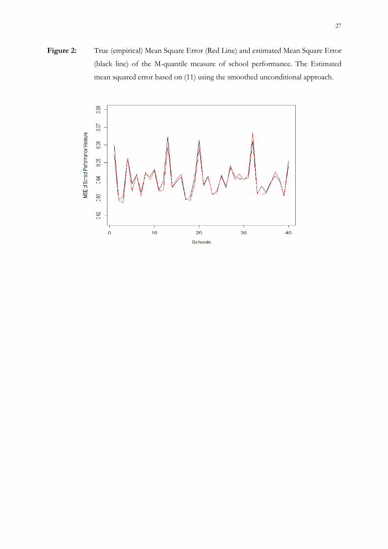
The results from this simulation studies are set out in Table 1 and Figure 2. The bootstrap MSE

estimator tracked the true (empirical MSE over Monte-Carlo simulations) MSE of the M-

quantile measure of school performance and provided coverage rates that were close to the

nominal 95%. On average, the relative bias was very low (1%-2%) and for the majority of the

schools this bias did not exceed 5%. The maximum relative bias was 14%, however, relative

percentage figures must be interpreted with care in this case as the MSE estimates are small

values. This is apparent by looking at the numbers of the actual and estimated MSEs for the

school with the highest relative bias. This is school 34 and the estimated MSE is 0.0366 whereas

the actual (Monte-Carlo) MSE is 0.032. These results suggest that the non-parametric bootstrap

scheme we proposed in Section 4 can be reliably used for estimating the MSE of the M-quantile

measure of school performance.

17

[Table 1 Here]

[Figure 2 Here]

5. Modelling Pupil Performance across London

In this section we now turn to the full application of the approach to pupils in schools in

London. We utilise the linked NPD/PLASC data to provide information on pupils background,

their performance at age 11 (prior attainment) and their performance at age 16 (the outcome).

To make the demonstration more straightforward we start with the 81,882 pupils that are sitting

exams within the right cohort (age 16 during the 2007/08 academic year). We then select those

that have performance information at both time-points (we lose just under 10,000 pupils), linked

PLASC data to provide the background information (we lose just under 5,900 pupils), and finally

we drop three schools that each contain a single pupil. This leaves us with 66,209 pupils.

5.1. Modelling the Pupil Performance

For the purposes of showing what can be achieved with this approach, we utilise a model

specification similar to the CVA model outlined in Ray (2006) and readers should refer to this

for a detailed motivation of the model specification. The outcome (pupil performance at 16) is a

score based in the pupils eight best exams. These are typically GCSEs (the standard exam taken

at age 16 at the completion of compulsory education in England) and eight GCSEs with top

grades of A* give a total score of 464. Pupils can exceed this maximum by taking exams in a few

subjects at a more advanced level at age 16 but for most pupils this creates a cap to their

performance measure. Prior attainment at age 11 is captured by the pupils mean performance

across Mathematics, English and Science (which has a quadratic relationship through the

inclusion of a squared term) as well as the differences between the pupil’s mean and their

individual scores in Mathematics and English. We also control for the school level mean in prior

attainment and the standard deviation of pupil prior attainment within school. (For simplicity, we

use the pupils’ mean prior attainment at age 11 to calculate these school level variables while Ray,

2006 uses a measure at age 14.) To control for pupil background we include an indicator for

receipt of free school-meals as a proxy for the pupil coming from a low income family, an

18

indicator of local area income for the pupils’ home address, as well as indicators of the pupils’

age within the school year, gender, ethnicity, first language at home, special educational needs,

and movement across local authority boundaries between ages 11 and 16.

5.2. Brief Discussion of the fitted Models

The motivation behind this paper is not to define a revised model specification at the pupil level

for contextual value-added modelling of school performance, but rather propose an alternative

framework in which to explore the schools’ performance. However, to demonstrate that the M-

quantile modelling is behaving as would be expected, Table 2 compares the model parameters

from the standard CVA approach (two-level random intercepts model with pupils within

schools) against the M-quantile median line.

[Table 2 Here]

From Table 2 we can see the same pattern emerging for both models, such as the lower

performance (conditional on all other factors) for those pupils receiving free school meals. Some

of the effects, while in the same direction are less pronounced in the median model such as the

quadratic shape for the average prior attainment, which may indicate the presence of some

outliers in the data. Standard errors are provided with both models. We should note that while

the random effects model has adjusted its standard errors for correlation within schools the M-

quantile model has not (and so its standard errors are likely under-estimated). This is not an issue

for the performance measure as the grouping structure is taken into after estimating the

individual efficiencies and the bootstrap approach we use (outlined in Section 4) does account

for the appropriate structure. However, it does raise the importance issue of model fitting and

the specification of the model structure, which we have not dealt with here given we are

reproducing the standard CVA model.

6. Evaluating the School and Local Authority Impact

In this section, we now use the results from the pupil level modelling in Section 5, which results

in the i

q ’s for each individual pupil being estimated, to construct a measure of school

19

performance (see Section 3.2) as well as exploring within schools and at a higher level of

aggregation comparing across the local authorities in London.

6.1. School Performance

We define the school performance as the mean of the pupils’ i

q ’s and as this moves away from

the overall pupil mean of 0.52 it represents the school adding to the efficiency of the pupils or

reducing the efficiency of the pupils. Of course, to judge this we need a confidence interval

around the school efficiency measure and this can be calculated via an estimated standard error

resulting from the bootstrap (see Section 4). These confidence intervals can be adjusted to allow

for multiple pair-wise comparisons between schools (Goldstein and Healy, 1995) but here we

just present estimates with standard 95% confidence intervals to illustrate the approach. Figure 3

presents this information as a caterpillar plot for six mixed schools from across London with a

range of estimated school efficiencies. The schools were chosen to have relatively small errors on

the overall q’s to demonstrate the potential impacts that can be seen across schools.

[Figure 3 Here]

As is common in these situations (see for example Leckie and Goldstein, 2009), the width of

these 95% confidence intervals demonstrate how careful we should be regarding comparing

schools to the overall mean or comparisons between schools (for which adjusted confidence

intervals would be needed). In addition, as these are mixed schools the efficiency of the school

has been calculated separately for boys and girls with corresponding standard errors and

confidence intervals. As the sample sizes for these gender specific efficiencies are smaller the

confidence intervals of course become correspondingly wider. This makes finding truly

significant differences difficult but interestingly in five of the six schools the school efficiency for

girls is higher, and this is after we have controlled for gender at the individual pupil level.

6.2. Comparing Performance across Local Authorities

Our modelling approach at the pupil level does not apriori impose a structure on the data and

this then allows us to produce an average performance measure at the local authority level

20

(averaging the pupils’ i

q ’s across local authorities rather than individual schools). However, the

bootstrap outlined in Section 4 samples pupil residuals within schools when applied at the school

level and so to produce standard errors at the local authority level we re-run the bootstrap

respecting this structure rather than the school structure.

We compare across the local authorities by mapping the average q’s. Figure 4a is the marginal

performance of each local authority based on averaging the pupils’ i

q ’s from a null (intercept

only) model so that we are comparing like with like. When making these comparisons and

interpreting the measures it is important to remember the M-quantiles do not exactly match the

empirical distribution so the empirical mean and median are not usually 0.5. The four colours

represent a group of local authorities clearly below the marginal mean for the pupils, one

spanning the mean (around 0.53), and two above the mean showing the positively skewed nature

the performance measures. Figure 4b is the conditional or ‘contextual value-added’ performance

mapped using the same legend to allow easy visual comparison.

[Figure 4 Here]

Comparing the two maps clearly shows less variation across the local authorities, once pupil

background and context has been controlled. In particular, the highest performing group on the

marginal map does not exist on the conditional map. In addition, the large area of poor

performing local authorities east of central London on the marginal map have all generally

improved once the controls are introduced. However, these conditional performance measures

are still subject to variability and therefore Figure 5 uses three colours to highlight those local

authorities with performance significantly above the overall mean of the conditional q’s (0.52),

those significantly below, and those in the middle based on whether the estimated 95%

confidence interval around the local authority estimates includes the overall mean.

[Figure 5 Here]

Figure 5 reveals two areas in south London that can be considered significantly below the mean

and across London there are some areas significantly above, but many cannot be considered

different from the mean. This again warns against simply ranking based on the q’s due to the

uncertainty.

21

7. Discussion

In this paper we have introduced an alternative framework for assessing the impact of schools

on their pupils’ performance. The standard approach to contextual value-added modelling uses a

random effects model to account for the residual impact of the school. However, this approach

makes fairly strong distributional assumptions and leads to a single measure. More complex

comparisons require more complex structures within the models. Our alternative approach

utilises the robustness of M-quantiles and as it leads to a measure of efficiency for the individual

pupils we can summarize performance at a variety of levels without requiring additional structure

in the modelling. We have chosen to use the mean, but as we have modelled the entire

distribution of performance, we can produce other summaries such as the proportion of pupils

within schools coming in the top 25% of the overall distribution to highlight schools that

particularly contribute to top pupil’s having high efficiency.

To explore a differing impact of the school by gender within the multilevel framework would

require a random slope at the school level on gender. Unlike our approach, this would give an

overall impact of gender differences at the school level but to do this imposes a structure in

relation to the variance of the school level random effects by gender. The approach we have

used here does not impose any overall structure (we cannot say there is a general impact of

gender on school effects) but is therefore flexible in terms of the actual impacts at the level of

the individual school. However, with both approaches finding significant impacts within

individual schools will likely be difficult due to the uncertainty across pupils at this level, as

shown in Figure 3. Exploring higher level impacts, such as the local authorities we have looked

mapped (Figures 4 and 5), can again be achieved within the multilevel framework by extending

the fitted model to include the extra level. However, as our approach has estimated the efficiency

at the pupil level we can explore the impact of this level without the need for additional

modelling.

One issue we should acknowledge is that of model fitting. In this work we have utilised a similar

model specification to the standard CVA model (Ray, 2006) and so standard errors on the model

parameters were not needed to judge the model specification. However, standard errors are

produced with each model (Table 2 presents them for the median) but, as noted in section 5,

these will not be adjusted to account for any higher level clustering in the data. The issue of

22

appropriate standard errors for model parameters is therefore a future area of research, although

the standard errors on the performance measures calculated via the bootstrap do adjust for

clustering in the population so that Figure 3 and 5 do give a fair picture of quality, given a model

specification.

References

Bowman, A.W., Hall, P. and Prvan, T. (1998). Bandwidth selection for the smoothing of

distribution functions. Biometrika, 85, pp 799-808.

Breckling, J. and Chambers, R.L. (1988). M-quantiles. Biometrika, 75, pp 761-771.

Chambers, R.L. and Tzavidis, N. (2006). M-quantile models for small area estimation. Biometrika,

93, 255-268.

Garner, C. L. and Raudenbush, S. W. (1991) Neighbourhood effects on educational attainment: a

multilevel analysis. Sociology of Education, 64, pp 251-262.

Goldstein, H., Rasbash, J., Yang, M., Woodhouse, G., Pan, H., Nuttall, D. and Thomas, S. (1993)

A multilevel analysis of school examination results. Oxford Review of Education, 19, pp 425-433.

Goldstein, H. (2003) Multilevel Statistical Models, 3rd edition, London: Arnold.

Goldstein, H., Burgess, S. and McConnell, B. (2007) Modelling the effect of pupil mobility on

school differences in educational achievement. Journal of the Royal Statistical Society A, 170, pp

941-954.

Goldstein, H. and Thomas S. (1996) Using Examination Results as Indicators of School and

College Performance. Journal of the Royal Statistical Society A, 159, pp 149-163.

Goldstein, H. and Speigelhalter D. (1996) League Tables and Their Limitations: Statistical Issues

in Comparisons of Institutional Performance. Journal of the Royal Statistical Society A, 159, pp

385-409.

Haveman, R. and Wolfe, B. (1995) The Determinants of Children’s Attainments: A Review of

Methods and Findings. Journal of Economic Literature, 33, pp 1829-1878.

Koenker, R. and Bassett, G. (1978). Regression quantiles. Econometrica 46, pp 33-50.

Koenker R. and D’orey, V. (1987). Computing regression quantiles. Journal of the Royal Statistical

Society C, 36, pp 383-393.

Kokic, P., Chambers, R., Breckling, J. and Beare, S. (1997) A Measure of Production

Performance. Journal of Business and Economic Statistics, 15, pp 445-451.

Leckie, G. and Goldstein, H. (2009) The limitations of using school league tables to inform

school choice. Journal of the Royal Statistical Society A, 172, pp 835-851.

23

Leckie, G. (2009) The complexity of school and neighbourhood effects and movements of

pupils on school differences in models of educational achievement. Journal of the Royal

Statistical Society A, 172, pp 537-554.

Li, Q. and Racine, J.S. (2007). Nonparametric Econometrics: Theory and Practice. Princeton: Princeton

University Press.

Lombardia M.J., Gonzalez-Manteiga W. and Prada-Sanchez J.M. (2003). Bootstrapping the

Dorfman-Hall-Chambers-Dunstan estimator of a finite population distribution function.

Journal of Nonparametric Statistics, 16, pp 63-90.

Mosteller, F. and Tukey, J. (1977), Data Analysis and Regression, Addison-Wesley.

Newey, W.K. and Powell, J.L.(1987). Asymmetric least squares estimation and testing.

Econometrica, 55, pp 819–47.

Ray, A. (2006) School Value Added Measures in England. Paper for the OECD Project on the

Development of Value-Added Models in Education Systems. London, Department for

Education and Skills http://www.dcsf.gov.uk/research/data/uploadfiles/RW85.pdf.

R Development Core Team (2008). R: A language and environment for statistical computing. R

Foundation for Statistical Computing, Vienna, Austria. ISBN 3-900051-07-0, URL http://www.R-

project.org.

Tzavidis, N., Marchetti, S., and Chambers, R. (2010). Robust estimation of small area means and

quantiles. Australian and New Zealand Journal of Statistics, 52, pp 167 - 186.

Tymms, P. and Coe, R. (2003) Celebration of the Success of Distributed Research with Schools:

The CEM Centre, Durham. British Educational Research Journal, 29, pp

Venables, W.N. and Ripley, B.D. (2002). Modern Applied Statistics with S. New York: Springer.

24

Table 1

Across schools distribution of the true (i.e. Monte Carlo) mean squared error, average over

Monte Carlo simulations of estimated mean squared error, relative bias (%) of the bootstrap

MSE estimator and coverage rates of nominal 95% confidence intervals for the M-quantile

measure of school performance (5).

MSE Percentiles of across schools distribution

Min 25th 50th Mean 75th Max

True 0.027 0.033 0.040 0.041 0.044 0.067

Bootstrap 0.028 0.034 0.040 0.041

0.043

0.065

Relative Bias (%) -7.27 -2.21 0.98 2.01 5.04

14.51

Coverage 0.928 0.940 0.948 0.952 0.961 0.984

The estimated mean squared error is based on (11) using the smoothed unconditional approach.

Intervals were defined as the M-quantile measure of school performance estimated by (6) plus or

minus twice its estimated standard error, calculated as the square root of (11).

25

Table 2

Comparison of the coefficients from the standard random effects approach to CVA with the

coefficients from the median M-quantile model

CVA Model M-quantile Median Model

Variable Estimate Standard

Error

Estimate Standard

Error

Const 151.52 24.80 110.08 8.76

KS2. Average Score (fine grade) -4.19 0.55 -1.42 0.45

KS2 Average Score (squared) 0.31 0.01 0.26 0.01

KS2 Difference from Average

(English) 0.36 0.08 0.40 0.06

KS2 Difference from Average

(Mathematics) 0.23 0.09 0.22 0.07

Pupil receives Free School Meals -7.55 0.64 -5.08 0.53

IDACI Score

(Pupil's Home Address) -30.09 1.56 -24.29 1.14

Pupil is Male -13.13 0.57 -13.67 0.40

Age within School Year -0.80 0.07 -0.69 0.06

English As First Language -16.47 0.82 -13.83 0.65

Not SEN Ref Ref

sen1 -39.43 1.63 -33.36 1.35

sen2 -35.18 0.66 -26.26 0.52

White British Ref Ref

White Other 14.57 1.06 15.93 0.85

Black African 23.88 1.02 21.34 0.82

Black Caribbean 9.45 1.02 7.86 0.81

Black Other 11.53 1.71 9.60 1.40

Indian 22.31 1.27 21.88 0.97

Pakistani 18.72 1.52 17.39 1.20

Bangladeshi 21.47 1.65 18.69 1.21

Chinese 32.18 2.75 28.67 2.28

Asian Other 28.43 1.58 27.26 1.29

Mixed 5.59 1.00 5.77 0.82

Other 21.69 1.43 23.00 1.16

Unknown 4.66 4.15 9.73 3.45

Different LA (KS2 to KS4) -2.21 0.62 -0.27 0.48

School Mean (KS2 Average Score) 3.41 0.68 3.48 0.18

School Standard Deviation

(KS2 Average Score) -1.67 1.59 -1.00 0.38

26

Figure 1: Comparing the fitted mean line (red) with fitted lines (grey) covering quantiles at

1%, 5%, 25%, 50%, 75%, 95% and 99%.

27

Figure 2: True (empirical) Mean Square Error (Red Line) and estimated Mean Square Error

(black line) of the M-quantile measure of school performance. The Estimated

mean squared error based on (11) using the smoothed unconditional approach.

28

Figure 3: Caterpillar plot for school comparing males and females

29

Figure 4: Mapping pupil performance across the Local Authorities of London

a) Mapping the mean of the marginal q values for pupils

b) Mapping the mean of the conditional q values for pupils

Excluded

0.44 - <0.50

0.50 - <0.54

0.54 - <0.60

0.60 - <0.67

Excluded

0.44 - <0.50

0.50 - <0.54

0.54 - <0.60

30

Figure 5: Highlighting Local Authorities with a mean q-value significantly above the overall

pupil mean (overall mean not within the estimated 95% confidence interval for

the Local Authority mean)

Excluded

Below

Expected

Above