quantifying and setting off network performance network performance... · quantifying and setting...

Int. J. Networking and Virtual Organisations, Vol. 3, No. 3, 2006 317

Copyright © 2006 Inderscience Enterprises Ltd.

Quantifying and setting off network performance

Erik Hofmann Kuehne-Institute for Logistics, University of St. Gallen, Dufourstrasse 40a, St. Gallen 9000, Switzerland E-mail: [email protected]

Abstract: While many aspects of the network and the collaboration process have been discussed in management literature, quantifying and setting off the network performance have remained largely unconsidered. Network performance management is an important arena for inter-organisational interaction. Therefore, a newly developed Shareholder Value-Added (SVA) transfer model will make a contribution to ease and support improvements in network management as well as to give specific guidelines and examples for its implementation. This paper also explains the inter-relationship between network decisions and the bottom line of the firm.

Keywords: performance metrics; Shareholder Value (SV); Discounted Cash Flows (DCFs); transfer payments; supply chain and network management.

Reference to this paper should be made as follows: Hofmann, E. (2006) ‘Quantifying and setting off network performance’, Int. J. Networking and Virtual Organisations, Vol. 3, No. 3, pp.317–339.

Biographical notes: Dr. Erik Hofmann is a Lecturer in Logistics Management at the University of St. Gallen, Switzerland. He is the Project Manager and Head of team ‘Training and Education’ at the Kuehne-Institute for Logistics, University of St. Gallen. He is also the General Manager of the Executive MBA in Logistics Management. He received his PhD in Industrial Engineering and Operations Management from the Darmstadt University of Technology, Germany. He teaches undergraduate and MBA courses in Supply Chain Management, Business Analysis and Logistics. His research areas of interest include mergers and acquisitions in the logistics industry, supply chain management and collaborations, strategy process research and collaborative working capital management.

1 Introduction

The interest in managing networks is growing rapidly among companies around the world. A major force behind this development is the belief that in networks working cooperatively can create a competitive advantage. Detecting the potential which is inherent of collaborating networks also means quantifying it. A system made up of indicators for assessing the potential value added in networks is not only needed to allocate resources to the most powerful instruments it contains, it is also vital for the survival of the network approach in practice (Baiman et al., 2001; Hofmann, 2005). Bowersox et al. (2000) expressed that unless the fact that managers can quantify the

318 E. Hofmann

operational and financial benefits of their supply chain initiatives, senior management, the market and shareholders will be hesitant to support them. Thus, it seems to be paramount to communicate why the network approach is useful and – more precisely – how useful it is. No CEO will allocate time and money to an approach that does not have an impact to the bottom line of the firm. But operational or financial processes do not have usually a directly visible link to a company’s overall performance. Therefore, it is the task for performance management to bridge the gap between operational and financial processes on the one side and management on the other side. In order to do this, performance management has to track the relevant performance indicators and condense them into those bottom line measures and indicators that management is interested in Lambert and Pohlen (2001).

In this paper, a model for quantifying and setting off network performance is developed. At the end, the network performance can be translated by transfer payments between the collaborating actors and Shareholder Value (SV). In Section 2, we describe the problem with current performance metrics and the need for network performance measures. Section 3 encompasses a discussion of the special aspects of SV applications in networks. It also describes the direct and the ceteris-paribus approach, deriving the SV in networks. Section 4 provides an introduction to a payment transfer system and shows how to put this concept into action. Some exemplary insights are presented in Section 4.3. Finally, Section 5 provides summarising remarks and suggestions for future research.

2 Performance metrics in networks and SV

2.1 How perspective leads to goals, which leads to measures

Using financial performance metrics to measure the impact of collaborations on company performance seems to be quite natural. In this paper we are choosing the SV approach as a framework and cash flow as the main performance driver. Ultimately to do so, there are some points to notice, which have considerable influence on our results. The reader should be aware of these implications when looking at collaborating networks from a SV perspective only.

One can distinguish between different perspectives on how to look at networks, whereas a perspective is a unique view towards an object that has to be analysed. It can further be described in terms of the perceived nature of the object, the standard problem and the standard solution it considers (Otto and Kotzab, 2003). Underlying these ‘schools of thought’ are disciplinary differences in core assumptions, norms and priorities (Lane et al., 1999). Priorities, or what is perceived as to be relevant, depend on goals (Otto and Kotzab, 2003). Thus we will ask: ‘Do collaborations pay?’ The answer depends on our perspective: collaborations pay, if they reach the set goals (Beamon, 1999).

Performance in a management context can never have a stand-alone existence. It is always assessed in relation to certain goals, which are usually equal to the company’s goals. In order to establish a sound basis for measuring network performance, one has to identify first the goals or goal structure (Otto and Kotzab, 2003). Beamon (1999) notes that, people in an organisation will concentrate on what is measured. Following this thought, we can conclude that performance measurement has a deep impact on the company’s direction. Both arguments lead to the same conclusion. It is of ultimate

Quantifying and setting off network performance 319

importance to link performance measurement with network strategy via a causal relation. The steering of collaborations requires that a performance metric, derived from network goals, exists (Neely et al., 1995).

The two notional steps we just pointed out can be combined into one line of arguments saying that the chosen perspective predetermines goals, which then lead to a certain set of performance metrics. This is the framework or ‘paradigm’ that we are using for the following sections.

2.2 Conventional performance measurement and their shortcomings

Performance measurement emerged as a reaction to the criticism on the accounting-focused ‘traditional’ measurement instruments, which have been developed in controlling literature. The role of ‘modern’ controlling for measuring performance in a network environment is not fixed neither in theory nor in practice. This is mainly due to lack of communication between the controlling and value chain-concerned functions. On top of that inter-organisational approaches (e.g. the supply chain management approach) are not yet implemented in the controlling frameworks. The main task of performance measurement is to choose the right performance metrics and indicators. It is therefore a part of the more encompassing performance management approach, which tries to link value-based strategy planning with measurement-based strategy implementation (Eccles and Pyburn, 1992; McNann and Nanni, 1994; Vitale and Mavrinac, 1995).

Beamon (1999) concludes that an effective performance measurement system will have to meet certain criteria in order to serve its purpose. These criteria for choosing or developing the right performance metrics in general and in a network context in particular are presented in Table 1.

Table 1 Characteristics of performance measurement systems

Characteristic General meaning Specific meaning in the network context

Inclusiveness Measurement of all pertinent aspects

• Contemplation of current and future aspects

• Consideration of network’s flow orientation

• Top-level-indicator carries a bottom line implication for top management

Universality Allow for comparison under various operating conditions

• Allow multi-level measurement

• Indicators must be built upon each other hierarchically and meaningful at all levels: organisational subunits, company-level and inter-organisational (network) level

Measurability Data required are measurable

Inter-organisational applicability: required indicators are measurable at all three levels

Consistency Measures consistent with organisation goals

Measures are consistent with network, collaboration and companies’ goals

The performance metrics and indicators provided by the pooled perspectives presented above are manifold and to discuss them here individually would be beyond the scope of this paper. Despite this wide set of choices there seems to be a general agreement between authors concerned with the topic that these traditional systems and indicators are not suitable for a network environment (Hieber, 2002; Lambert and Pohlen, 2001).

320 E. Hofmann

Commonly cited critics about the traditional performance measures are (Beamon, 1999): they are not inclusive; they are concerned with company-internal process and functions, thus loosing their meaning when used in an inter-organisational context and they are often inconsistent with strategic goals.

Farris and Hutchison (2003) point out that only very few indicators can be combined into a more integrated view by simply adding the corresponding metrics of subsequent network entities, for example, cash-to-cash cycle time, total inventory or response time. Although these imperfections are apparent for practitioners companies still have problems in developing meaningful performance metrics, which can be used for network performance management. These difficulties exist not only due to a lack in network orientation of the respective companies but – in addition to that – problems arise of the complexity of capturing metrics across multiple companies, an unwillingness to share relevant information, and inability to capture performance at the necessary customer-, product- or network/supply chain-level. Many measures identified as supply chain metrics are for example actually measures of internal logistics operations as opposed to genuine supply chain metrics. Lambert and Pohlen (2001) conclude that inventory turnover, which is a common indicator for conventional logistics performance, looses its meaning when applied in a multi-company context. The reason therefore is that the further the inventory is located on an upstream position; the lower is usually its attached cash value. Due to this, the inventory turnover rate of a supplier is not comparable with the turnover rate of a company further down the supply chain. Since we are concerned about the financial activities within a network we will have a closer look at financial performance measures in particular.

Even more popular than liquidity or cost indicators, profitability, especially Return on Investment (ROI) and Return on Equity (ROE) is cited to be the most popular financial performance measure in Western companies. But the flaws of traditional accounting-based measures as opposed to cash flow are apparent. According to Mills and Chen (1996); they are subject to (legal) accounting manipulation and policies, varying across different national boundaries; they are backward looking and they are focused on short-term results.

Rappaport (1998) argues that accounting-based distortion may result from inflation, the depreciation method, lifetime of the assets, mix of fixed assets, off balance sheet assets, off balance sheet debt, goodwill, asset revaluation, cross-holdings, retained earnings or consolidated balance sheets. Profitability-based indicators have the additional drawback of not considering the assets that were needed to create the respective profit. As a result seemingly profitable companies might actually be destroying value because their post-tax operating income does not cover the true cost of capital (Christopher and Ryals, 1999).

2.3 Implications of and reasoning for a SV perspective

The drawbacks associated with traditional financial performance measures led to the need of a new financial approach for measuring company performance: the concept of Value-Based Management (VBM) is expressed through the SV approach. It states that real value as opposed to paper profits is only created if an organisation generates returns that fully compensate investors for the total cost involved in the investment, plus a premium which more than compensates for the risk incurred (Christopher and Ryals, 1999). The idea is based on the Capital Asset Pricing Model (CAPM), which describes


the market trade-off between risk and return in an investment portfolio (Coyle, 2000; Deimel, 2002; Emery and Finnerty, 1991). While SV is the financial value created for shareholders by companies in which they invest, VBM is concerned with the strategies by which this SV is generated (Christopher and Ryals, 1999). Sustainable SV can only be created through value-based thinking and acting on all levels of an organisation.

Unlike many operating performance measures commonly used in other disciplines, financial figures are the most common indicators for showing the overall corporate performance (Lalonde, 2000). A study conducted by the European Logistics Association and Bearing Point (2002) revealed the existence of a growing importance to measure financial supply chain management indicators on a corporate level (Hofmann, 2003, 2005). Apparently measuring financial performance indicators on a corporate level can be used to connect the different corporate levels within a network. Measuring these indicators is thus a very efficient way to move the network approach from the backroom to the boardroom (Timme and Williams-Timme, 2000).

But why should the collaborating partners use the SV approach as their ultimate guidance system? Singhai and Hendricks (2002) give four answers: firstly, SV is not subject to the traditional accounting-based measurement flaws mentioned above. Secondly, when calculated the right way, it provides information about the condition of all levels within a company and about the network. Thirdly, it gets more and more attention especially from the top management. Last but not the least, it consistently aligns financial goals in terms of a coherent shareholder orientation on all levels.

Basically the SV approach is explicitly focussing on generating value for shareholders (Christopher and Ryal, 1999; Deimel, 2002). Other stakeholders, such as employees, suppliers or customers are only regarded as something that has to be considered necessarily to get closer to the final goal of creating value for shareholders (Berman et al., 1999). In the end all group of stakeholders have a long-term interest in preserving and increasing the company value.

But there are not only ‘pros’ but also some ‘cons’ in using the SV approach. First of all the considerable complexity of calculation should be mentioned (Christopher and Ryals, 1999). This will especially become relevant when modifications need to be made to align the concept, which is initially concerned with single companies only, but now used for a multiple-enterprise network context. Further more, capital structure problems are not taken into account since the risk of fluctuations in future cash flows as well as the risk of bankruptcy are eliminated within the model (Casey, 2001).

2.4 SV on the basis of discounted cash flows

The increasing popularity of VBM has led to multiple approaches dealing with this concept, each of them having particular advantages and disadvantages for different purposes. We will use the Discounted Cash Flow (DCF) method that has been introduced by Rappaport (1998) to quantify the SV created by collaborations or entire networks. Apart from the DCF method, the other two VBM methods – the Economic Value-Added (EVA) method and the Cash Flow Return on Investment (CFROI) method (Christopher and Ryals, 1999) – will not be introduced in this paper.

Briefly the DCF approach to VBM can be described as a method that evaluates the recent and future liquidity of a company. Therefore it adjusts the expected cash flows, which are generated by a company’s operating activities, by the time value of money to get the corporate value. Then the corporate value will be reduced by the company’s debt.

322 E. Hofmann

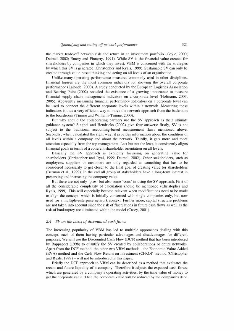
The result is the ‘true’ equity portion of the business and is called ‘SV’ (Rappaport, 1998). The basic idea of this approach is illustrated by Figure 1. The relevant formulas to calculate SV are presented in Formulas F1–F3, Appendix.

Figure 1 Basic DCF-equation for calculating SV

Probably the most complex and error-prone part of SV-calculation in the DCF method is the correct determination of future cash flows (Hertenstein and McKinnon, 1997). Not only the very nature of future predictions is subject to risk, but also the method of calculating cash flows by itself is subject to considerable dispute (Brealey and Myers, 2000). The root of the problem can be traced to the question whether an indirect calculation of cash flow based on information from the balance sheet, the income statement and side information, is sufficient or if a direct calculation by using payment transactions is absolutely required.

Finding an answer to this question is even more complicated, since practice and theory provide lots of different ways for an indirect calculation of cash flow. For now, we will suppose that a derivative approach that reveals the ‘true’ cash flow of a business given that the necessary information is available and reliable.

The term cash flow as used by Rappaport (1998) is delusive since in fact the DCF approach is not using a regular cash flow in the common understanding but the Free Cash Flow (FCF). The FCF is closely related to the cash flow though and represents the incremental cash at the end of a given period generated by the company’s turnover process. This is the cash flow that is free and available to be distributed to both the firm’s debt and equity investors (Keown et al., 2001). The FCF is most commonly calculated on the basis of the income statement consecutively applying several conversions in order to obtain a figure that is free of accounting flaws and as close to market values as possible. Although it might be argued that the mixed-method approach is methodically questionable, we will follow it here, primarily due to the lack of other practically accepted alternatives. Formula F2 displays the derivative calculation scheme for after tax FCF as we use it in combination with the DCF method (see Appendix). This method is in line with the works of Rappaport (1998), Booth (1998), Brealey and Myers (2000) and Keown et al. (2001). After calculating the FCF we are able to compute the SV (see Formula F3, Appendix).

As pointed out above, the single use of SV as our only performance indicator is not sufficient since there is no link to operational/financial processes. To take these process into account we need to break this top-performance-indicator down into pieces that are suitable for daily operations and decision-making. Rappaport (1998) identifies seven basic valuation parameters of SV that can be used to systemise a more detailed


calculation for a network-environment. These are the sales growth rate, operating profit margin, income tax rate, working capital investment, fixed capital investment, cost of capital and the forecast duration. Note that the overriding performance indicator thereby is no longer the total SV but instead the Shareholder Value Added (SVA).

The SVA is especially well-suited for performance measurement since it allows comparisons of different alternatives as well as a periodic perspective on the creation of SV. Further more the SVA is able to show the contributions of each member of the collaboration for different actions in the network. In fact the SVA is nothing more than the difference between two SVs of either different alternatives or periods. Therefore, the calculation of the SV is the first step in calculating the SVA. In the next step, we have to adapt the SV approach to our special context of collaborations.

3 Using the SV approach in a network environment

3.1 Special aspects of SV applications in networks

The SV concept is designed for single business or their subunits. To use this concept in a network environment it requires a modification to take inter-organisational aspects into account. The changes that are needed to design a network-wide performance system are superimposed by the changes that are covering the special aspects of collaborations. Next to the indirect effects of network performance indicators on financial goals of a company, the direct payments between the network members have to be considered. This is necessary since the collaborating network actors are influenced by contractual regulations not only concerning the quantity and delivery times of goods or services, but also the prices and payment policy. The financial flows within collaborations are determined by strategic decisions that have been made in the early forming stage of the network. Hence tracking and controlling of payments is an essential part of a network’s day-to-day business (Srivastava et al., 1998).

In a network, investors cannot be seen as a homogeneous group. Instead, shareholders of different network members have different preferences of risk and return. This leads to the fact that the single discount rate known from the original SV model no longer exists. The specific discount rates of the different collaboration entities are relevant and have to be regarded. However, the collaborating companies remain legally independent entities, which are only responsible for a delivery of value to their investors. The advantage of participating in the collaborating network soon has to be evaluated by every single member. This is not always reality in practice especially when a supplier is strongly linked to its customer. This case is often found in the automotive industry due to a focal OEM, who has the power to prescribe the rules of the relationship. However if the collaboration is not creating value to this supplier, both the network and the supplier might be better off without collaborating. In an environment where one focal network entity exists, value creation for the whole value chain can become more difficult.

Apparently the creation of value within a network is not a zero-sum game. Unlike other forms of relationships there is no central authority that has the concern and the power to push through those strategies and actions that maximise the overall value within collaborations (Ramdas and Spekman, 2000). Hence, the network must contain an instrument that aligns the overall collaboration’s with each member’s individual benefits. By transferring the collaboration’s overall value added into an individual value added for

324 E. Hofmann

each member this instrument also serves as an incentive for network members to participate actively in the collaboration (Baiman et al., 2001).

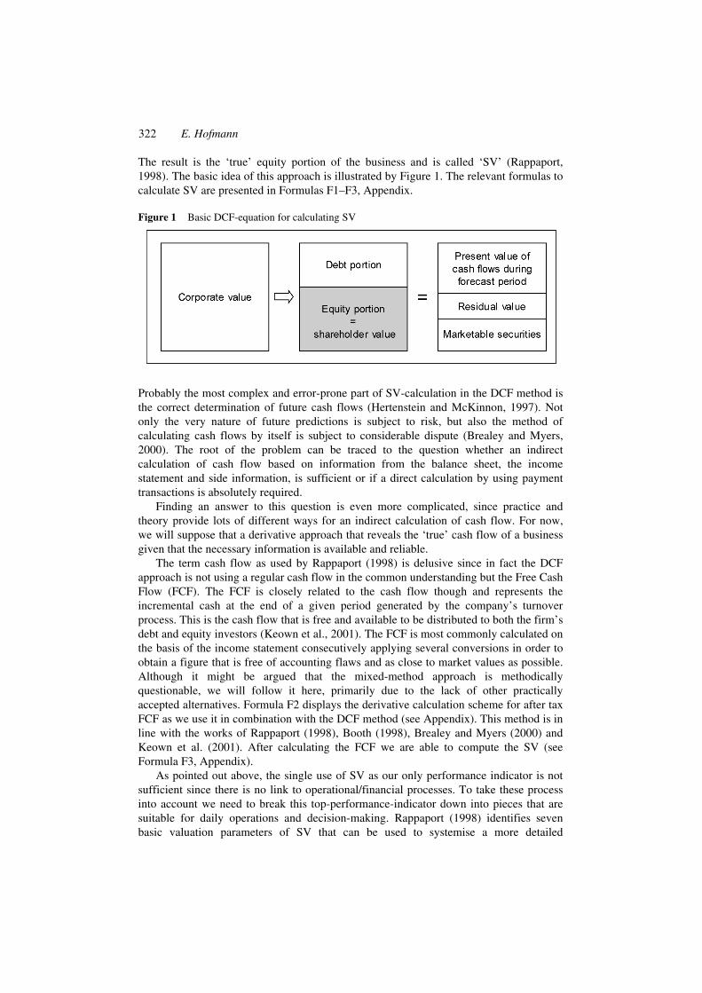
To determine whether a participation in the collaboration is advantageous, each entity will now be able to consider the expected cash inflows and outflows. A possible construct of cash in- and outflows is given in Figure 2.

Figure 2 Cash flows associated with the collaboration from an individual viewpoint

As already indicated in the figure the incentive sought to align the collaboration’s overall and each member’s individual goals can be provided by transfer payments between the entities. Ideally these transfer payments are based on objectively measurable criteria. Otherwise the participants will be induced to reveal false numbers, in order to receive higher transfer payments.

To summarise our thoughts, we need to develop a performance measurement system that:

• fulfils the generic performance measurement criteria

• explicitly tracks and controls the cash transactions between the collaboration members

• contains a system for transfer payments in order to align individual and collaborative goals

• is ideally based on objectively measurable figures, allowing a cross-checking of data between the members and

• is not influenced by decisions or actions that do not originate from the network.

3.2 Two ways for SV application in networks

There are two possible but essentially different approaches to create a performance measurement system in network environments on the basis of the SV: the first is a direct respectively bottom-up approach, which is measuring the network-related data for each collaboration member in a first step and combines it to a ‘network SV’ in a second step. The second is the indirect respectively ceteris-paribus approach, which is deriving the SV added by the collaboration on basis of each company’s overall SV. In the following section, we will argue why the direct approach is less useful and then further elaborate on the second approach.


Regarding the requirements stated above, the idea of using the captured collaboration-specific cash inflows and outflows of each member to calculate a figure seems to be straight forword. Applying the DCF method to the member-specific FCFs that are associated with the collaboration leads to the member-specific network SV. The combination of the network SV of each member results into an overall network SV. Unfortunately this direct approach, which is conceptually reasonable, is not very practicable. In business practice it might be very difficult to distinguish between network-related and non-network-related cash flows. While the tracking of payments to and from other collaboration members is fairly easy to realise other cash flows like wages, interest and taxes are much harder to link to network activities. Furthermore, the different capital structures of the collaboration members are leading to different SV contributions by each entity. This bears a huge conflict potential. For this reason the network SV can therefore not be a means to an end, but only a means for redistributing created value towards the collaboration members.

To overcome the many disadvantages of the DCF method we will now use the ceteris-paribus approach. It is based on the idea that if all other influences are ceteris-paribus, network-actions add SV to the collaboration members. Hence, comparing the SV after collaborative measures with the current state outcomes reveals a SV added for each member. The alternative maximising the overall SVA – that is the sum of all individual SVAs – seems to be the optimal choice.

How much value can be added is a question of how much value there is in the first place. Consequently, when thinking about entering a collaboration, that is the precollaborative state, the company will compare its single-entity (financial) situation with the projected collaborative outcome (note that collaboration are only considered as such after underwriting of the pertaining contracts). A mere market relationship is not considered collaborative. Later while being in existence, network measures have to convince the members in two ways: firstly, any new measure has to add value compared to the current collaborative situation. Secondly, each member will also weigh the two options: ‘What would I do if I would be on my own?’ and ‘What will we do collaboratively?’ In other words the collaboration members need to evaluate the stand-alone versus the collaborative alternative. Only if the collaborative choice delivers a superior outcome to each network member, the collaborative alternative will be chosen.

Since the SVA strategy generates the highest excess FCF, the extra cash can be redistributed towards the members in order to create a win–win situation for all parties. Gjerdrum et al. (2002) propose the use of a Nash-bargaining solution to obtain an equitable distribution of the profit, which is in our case excess cash created by the network. This approach contains the following advantages:

• a specific assignment of FCFs to the collaboration is no longer necessary since each company only calculates its overall (company-) SV

• the calculation of SV and SVA created through collaborations on company-level carries a bottom line implication not only for top management but also for investors (shareholders)

• the calculation of SV on company-level using the DCF method is possible with current (accrual-basis) accounting systems

• the SVA allows for an easy comparison of different alternatives and periods and

• the capital structures of the collaboration members as well as all other influences on SV are faded out.

326 E. Hofmann

What is considered as an advantage in easing the calculation might also be interpreted as a disadvantage in terms of transparency. Since the SVA approach abandons the effort to distinguish between direct collaborative cash flows and indirect effects on SV, the direct and indirect cash flow effects are not quantified. Instead the quantified figures are a result of mixed direct and indirect effects. Another weakness, that is common to all SV approaches, is the accurate prediction of future cash flows.

Basic requirement for this approach is the ability of each network member to calculate his own SV using a commonly agreed-upon method. Due to the many ways for indirectly calculating cash flows and FCFs, the members need to set up a detailed frameworks determining, which positions the cash flow consists of. Ideally these frameworks are provided by standard developing organisations like national or international associations (e.g. the Council of Supply Chain Management Professionals (CSCMP) or the European Logistics Association (ELA)).

Note that we do not say that the tracking of network-related payments between the collaboration parties is no longer necessary. This is still the foundation for controlling, steering and optimising the inter-organisational relationship between the partners. We rather follow a dual approach that is combining the advantages of both, the direct and the indirect cash flow method. This is on the one hand delivering the required precision and the instruments for efficiently steering the collaborative cash flows and on the other hand allowing a comfortable and widely accepted assessment and controlling of the results. The capturing of cash flows that are related to the network but do not flow between two or more entities is no longer necessary, an advantage greatly reducing the complexity of putting collaborating networks into practice. Instead, the ceteris-paribus approach realises that these cash flows have a direct influence on the SV of each member and that they are therefore completely accounted for in the SVA.

4 The collaborative SVA transfer model

4.1 A conceptual look behind the SVA transfer model

Starting point for the ceteris-paribus approach is a unified calculation of each collaborating firm’s FCFs and its SV. As we have seen, the calculation method that we use for deriving the FCF is based on the NOPAT (see Formula F2, Appendix). The ease of implementation and practicability of this method is subject to the quantity of the necessary conversions that need to be applied to the specific company.

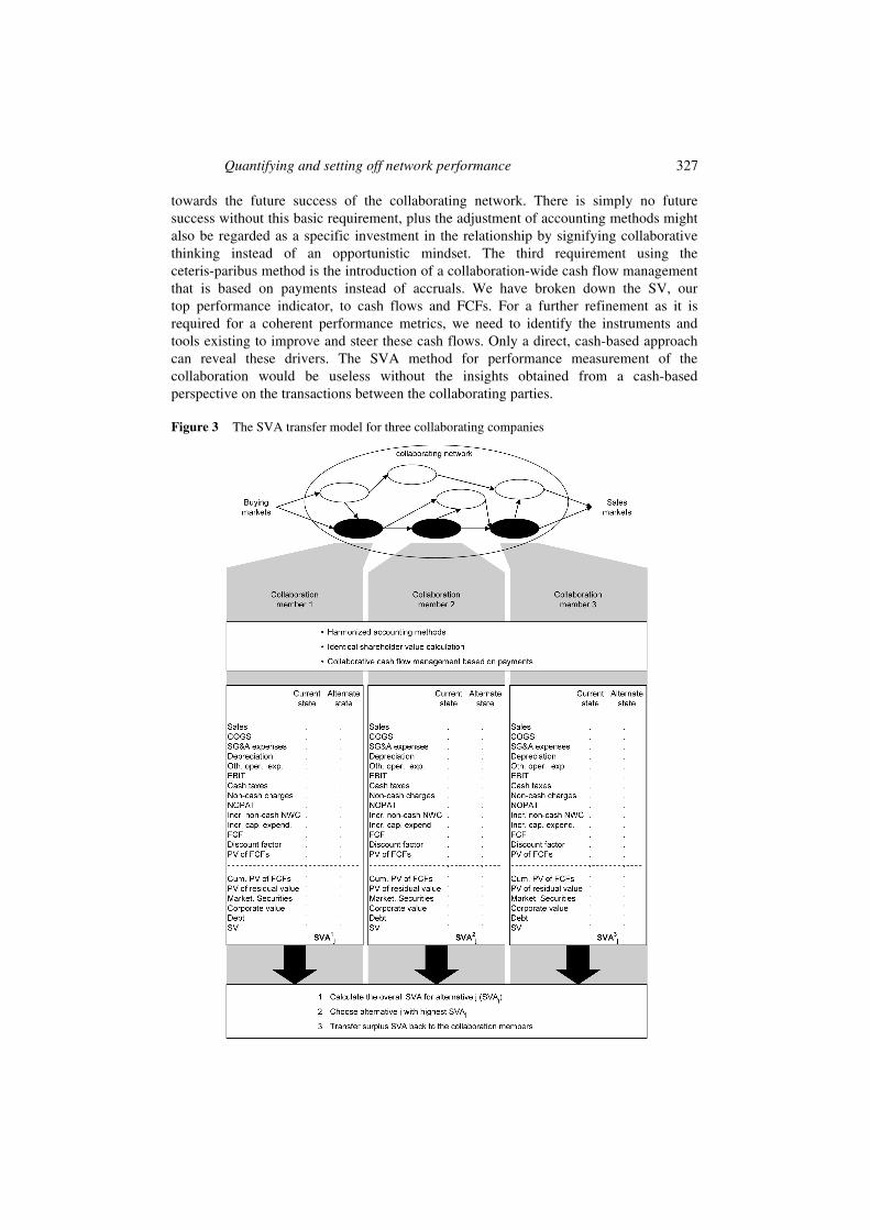
The basic idea behind the ceteris-paribus approach for collaborations between three firms of the same network/supply chain is illustrated in Figure 3. It is immediately visible that an agreement about the same SV calculation method is useless without a harmonisation of the accounting procedures as a first step. We do not say that the firms need to unify their accounting systems. Instead, they only need to make sure that all relevant positions that are accounted in the FCF calculation are based on identical rules and procedures. If any of the firms uses a different approach, for example in the accounting of its inventory, it needs to converse this figure in order to follow the rules required by the calculation method. The harmonisation of accounting methods and the necessary collection of side information and extra data certainly involve a huge effort for all parties. In fact, it might be seen as one of the main difficulties to implementing the collaboration approach. On the other hand, the willingness to abide to this necessity can be considered as a great deal of commitment and might be interpreted as a first indicator


towards the future success of the collaborating network. There is simply no future success without this basic requirement, plus the adjustment of accounting methods might also be regarded as a specific investment in the relationship by signifying collaborative thinking instead of an opportunistic mindset. The third requirement using the ceteris-paribus method is the introduction of a collaboration-wide cash flow management that is based on payments instead of accruals. We have broken down the SV, our top performance indicator, to cash flows and FCFs. For a further refinement as it is required for a coherent performance metrics, we need to identify the instruments and tools existing to improve and steer these cash flows. Only a direct, cash-based approach can reveal these drivers. The SVA method for performance measurement of the collaboration would be useless without the insights obtained from a cash-based perspective on the transactions between the collaborating parties.

Figure 3 The SVA transfer model for three collaborating companies

328 E. Hofmann

4.2 Putting the SVA transfer model into action

As indicated in the lower box of Figure 3, three consecutive steps are needed to evaluate the network performance and find the optimal collaborative strategy.

In the first step each of the collaborating companies calculates its current state SV on the basis of the FCF schemes (see Formulas F2 and F3, Appendix). The calculated current state SV is then compared to the forecasted SV that could be achieved if a certain collaborative strategy is chosen. The same scheme is followed when a new member enters the collaborating network. Comparing the current state (without the new participant) with the new situation where the company is a part of the collaboration leads to the SVA. Similar to any other activity, the entrance or exit of collaborating members can simply be seen as an additional strategy/alternative. A strategy/alternative in this context refers to a collaboration-specific set of actions. The actors in the collaboration can make choices between these strategies/alternatives to achieve various goals like process-changes, etc. Thus, different strategies/alternatives provide different solutions for the same question. For example, a supply chain collaboration might think about ways to improve its e-payment processes. So far, all e-payments have been handled by the network members themselves without any cooperation. According to the model, each actor has to calculate its current state SV first. Next, the financial impact of each alternative is quantified. Alternative 1 for example could be a proposal to outsource the collaboration-wide e-payments to a specialised payment service provider. This would have an impact on the associated yearly FCFs since costs, which have been so far associated with the maintaining of e-payments, like wages, fees for associated banking services, administrative cost, etc., will no longer exist. Instead, a constant cash outflow for paying the e-payment service provider has to be taken into account. Alternative 2 could refer to employing a different provider who offers additional services, leading to even less internal cost but higher fees for his services. Alternative 3 relates to the transfer of all collaborative e-payment activities to a specific member. Another good example is a warehouse localisation problem. In this case, Alternative 1 could describe a solution, where the warehouse will be built at a specific location and is operated by actor A. Alternative 2 could refer to a different situation, where the warehouse will be built at a different location and will be run by company B instead. Alternative 3 might involve shut the warehouse at still another location and outsourcing its management to a logistics provider, etc. Again, each alternative is associated with different future FCFs for the companies involved, leading to different SVs added and attached to each alternative.

Each alternative or strategy therefore possibly – but not necessarily – involves a different set of actions and leads to a different distribution of actual and future FCFs for each member. Consequently each alternative indicated by the index ‘j’, is usually associated with a different SVA for the individual actors. All strategies/alternatives are calculated on the assumption that all other variables possibly influencing the firm’s SV remains constant (‘ceteris-paribus approach’). Only the different figures that directly or indirectly result from the collaborative actions are taken into account. In the examples, only the earnings and expenditures directly or indirectly associated with e-payments or warehouse would change from alternative to alternative while all other figures remain constant. The difference between the calculated current state SV and the collaborative strategy SV then reveals the SVA of alternative j for each firm, SVA ,ij where ‘i’ is the

index for the participating collaborating members. If ‘i’ is omitted, we therefore refer to


the whole network that is the sum of all individual SVA .ij The sum of all members’

SVAs for alternative j represents the SVA added to the whole collaborating network by alternative j (SVAj).

The second step is to find the joint network strategy that maximises the overall SVA, which is the sum of all individual SVAs. Note that this might require some members to move away from the individual SVA-maximum at this point. If that is the case, the respective companies will get compensated later on with at least the same amount that they forgo at this point.

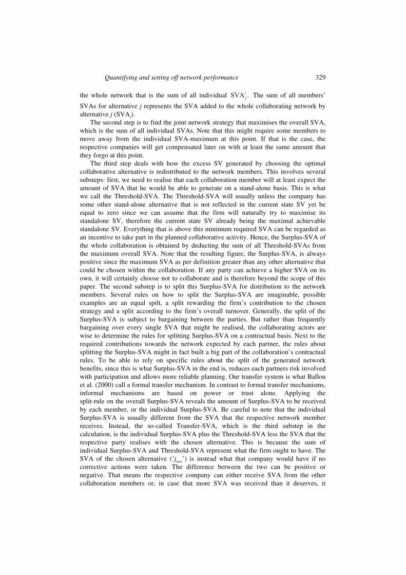
The third step deals with how the excess SV generated by choosing the optimal collaborative alternative is redistributed to the network members. This involves several substeps: first, we need to realise that each collaboration member will at least expect the amount of SVA that he would be able to generate on a stand-alone basis. This is what we call the Threshold-SVA. The Threshold-SVA will usually unless the company has some other stand-alone alternative that is not reflected in the current state SV yet be equal to zero since we can assume that the firm will naturally try to maximise its standalone SV, therefore the current state SV already being the maximal achievable standalone SV. Everything that is above this minimum required SVA can be regarded as an incentive to take part in the planned collaborative activity. Hence, the Surplus-SVA of the whole collaboration is obtained by deducting the sum of all Threshold-SVAs from the maximum overall SVA. Note that the resulting figure, the Surplus-SVA, is always positive since the maximum SVA as per definition greater than any other alternative that could be chosen within the collaboration. If any party can achieve a higher SVA on its own, it will certainly choose not to collaborate and is therefore beyond the scope of this paper. The second substep is to split this Surplus-SVA for distribution to the network members. Several rules on how to split the Surplus-SVA are imaginable, possible examples are an equal spilt, a split rewarding the firm’s contribution to the chosen strategy and a split according to the firm’s overall turnover. Generally, the split of the Surplus-SVA is subject to bargaining between the parties. But rather than frequently bargaining over every single SVA that might be realised, the collaborating actors are wise to determine the rules for splitting Surplus-SVA on a contractual basis. Next to the required contributions towards the network expected by each partner, the rules about splitting the Surplus-SVA might in fact built a big part of the collaboration’s contractual rules. To be able to rely on specific rules about the split of the generated network benefits, since this is what Surplus-SVA in the end is, reduces each partners risk involved with participation and allows more reliable planning. Our transfer system is what Ballou et al. (2000) call a formal transfer mechanism. In contrast to formal transfer mechanisms, informal mechanisms are based on power or trust alone. Applying the split-rule on the overall Surplus-SVA reveals the amount of Surplus-SVA to be received by each member, or the individual Surplus-SVA. Be careful to note that the individual Surplus-SVA is usually different from the SVA that the respective network member receives. Instead, the so-called Transfer-SVA, which is the third substep in the calculation, is the individual Surplus-SVA plus the Threshold-SVA less the SVA that the respective party realises with the chosen alternative. This is because the sum of individual Surplus-SVA and Threshold-SVA represent what the firm ought to have. The SVA of the chosen alternative (‘jmax’) is instead what that company would have if no corrective actions were taken. The difference between the two can be positive or negative. That means the respective company can either receive SVA from the other collaboration members or, in case that more SVA was received than it deserves, it

330 E. Hofmann

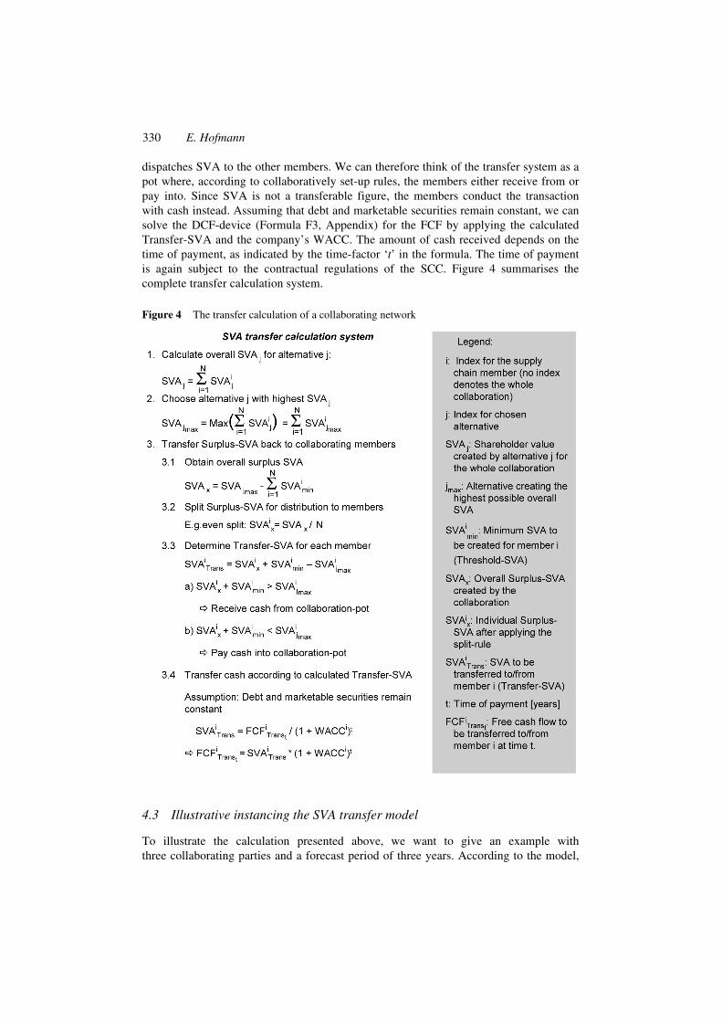
dispatches SVA to the other members. We can therefore think of the transfer system as a pot where, according to collaboratively set-up rules, the members either receive from or pay into. Since SVA is not a transferable figure, the members conduct the transaction with cash instead. Assuming that debt and marketable securities remain constant, we can solve the DCF-device (Formula F3, Appendix) for the FCF by applying the calculated Transfer-SVA and the company’s WACC. The amount of cash received depends on the time of payment, as indicated by the time-factor ‘t’ in the formula. The time of payment is again subject to the contractual regulations of the SCC. Figure 4 summarises the complete transfer calculation system.

Figure 4 The transfer calculation of a collaborating network

4.3 Illustrative instancing the SVA transfer model

To illustrate the calculation presented above, we want to give an example with three collaborating parties and a forecast period of three years. According to the model,


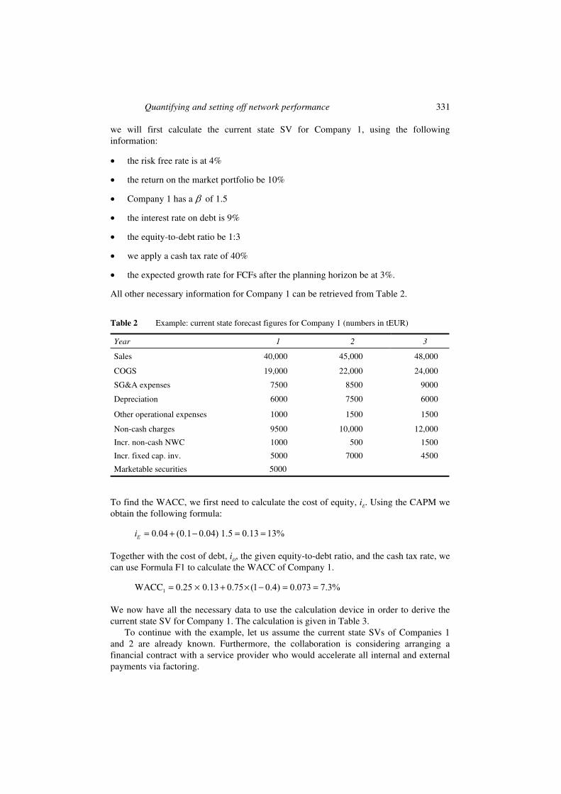
we will first calculate the current state SV for Company 1, using the following information:

• the risk free rate is at 4%

• the return on the market portfolio be 10%

• Company 1 has a β of 1.5

• the interest rate on debt is 9%

• the equity-to-debt ratio be 1:3

• we apply a cash tax rate of 40%

• the expected growth rate for FCFs after the planning horizon be at 3%.

All other necessary information for Company 1 can be retrieved from Table 2.

Table 2 Example: current state forecast figures for Company 1 (numbers in tEUR)

Year 1 2 3

Sales 40,000 45,000 48,000

COGS 19,000 22,000 24,000

SG&A expenses 7500 8500 9000

Depreciation 6000 7500 6000

Other operational expenses 1000 1500 1500

Non-cash charges 9500 10,000 12,000

Incr. non-cash NWC 1000 500 1500

Incr. fixed cap. inv. 5000 7000 4500

Marketable securities 5000

To find the WACC, we first need to calculate the cost of equity, iE. Using the CAPM we obtain the following formula:

0.04 (0.1 0.04) 1.5 0.13 13% Ei = + − = =

Together with the cost of debt, iD, the given equity-to-debt ratio, and the cash tax rate, we can use Formula F1 to calculate the WACC of Company 1.

1 0.25 0.13 0.75 (1 0.4) 0.073 7.3%WACC = × + × − = =

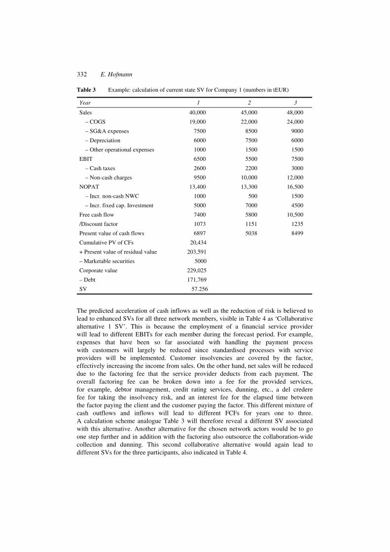
We now have all the necessary data to use the calculation device in order to derive the current state SV for Company 1. The calculation is given in Table 3.

To continue with the example, let us assume the current state SVs of Companies 1 and 2 are already known. Furthermore, the collaboration is considering arranging a financial contract with a service provider who would accelerate all internal and external payments via factoring.

332 E. Hofmann

Table 3 Example: calculation of current state SV for Company 1 (numbers in tEUR)

Year 1 2 3

Sales 40,000 45,000 48,000

– COGS 19,000 22,000 24,000

– SG&A expenses 7500 8500 9000

– Depreciation 6000 7500 6000

– Other operational expenses 1000 1500 1500

EBIT 6500 5500 7500

– Cash taxes 2600 2200 3000

– Non-cash charges 9500 10,000 12,000

NOPAT 13,400 13,300 16,500

– Incr. non-cash NWC 1000 500 1500

– Incr. fixed cap. Investment 5000 7000 4500

Free cash flow 7400 5800 10,500

/Discount factor 1073 1151 1235

Present value of cash flows 6897 5038 8499

Cumulative PV of CFs 20,434

+ Present value of residual value 203,591

– Marketable securities 5000

Corporate value 229,025

– Debt 171,769

SV 57.256

The predicted acceleration of cash inflows as well as the reduction of risk is believed to lead to enhanced SVs for all three network members, visible in Table 4 as ‘Collaborative alternative 1 SV’. This is because the employment of a financial service provider will lead to different EBITs for each member during the forecast period. For example, expenses that have been so far associated with handling the payment process with customers will largely be reduced since standardised processes with service providers will be implemented. Customer insolvencies are covered by the factor, effectively increasing the income from sales. On the other hand, net sales will be reduced due to the factoring fee that the service provider deducts from each payment. The overall factoring fee can be broken down into a fee for the provided services, for example, debtor management, credit rating services, dunning, etc., a del credere fee for taking the insolvency risk, and an interest fee for the elapsed time between the factor paying the client and the customer paying the factor. This different mixture of cash outflows and inflows will lead to different FCFs for years one to three. A calculation scheme analogue Table 3 will therefore reveal a different SV associated with this alternative. Another alternative for the chosen network actors would be to go one step further and in addition with the factoring also outsource the collaboration-wide collection and dunning. This second collaborative alternative would again lead to different SVs for the three participants, also indicated in Table 4.


Table 4 Example of potential SVs for the collaborating actors (numbers in tEUR)

Company 1 Company 2 Company 3

Current state SV 57,256 95,000 30,000

Max. stand-alone SV 57,256 95,000 33,000

Coll. alternative 1 SV 61,050 106,000 32,000

Coll. alternative 2 SV 63,000 99,000 35,000

While the current state SVs of Companies 1 and 2 also represent their maximum achievable stand-alone SVs, Company 3 actually has the option to increase its standalone SV to EUR 33,000,000 on its own, for example by improving its internal collection and dunning process. Its Threshold-SVA, that is the minimum SVA required to participate in any collaborative strategy is therefore EUR 3,000,000, while Companies 1 and 2 have a Threshold-SVA of zero. Each company’s SVA for the two collaborative alternatives is the alternative’s SV less the current state SV. By looking at the sum of generated SVAs, we find collaboration Alternative 1 to create the highest overall SVA of EUR 16,794,000. The overall current state SV is [tEUR] 57,256 + 95,000 + 30,000 = 182,256. Alternative 1’s SV is [tEUR] 61,050 + 106,000 + 32,000 = 199,050. Alternative 1’s SVA therefore is [tEUR] 199,050 − 182,256 = 16,794. The overall Surplus-SVA is therefore EUR 16,794,000 − EUR 3,000,000. For simplicity reasons, we distribute this excess SVA equally towards the collaboration members, giving each of them a share of EUR 4,598,000.

To get the Transfer-SVA, we add the Threshold-SVA to the Surplus-SVA and then deduct the amount the company will receive if the maximum alternative is followed, which in this example is SVA1. This Transfer-SVA is then converted into cash assuming a payment period of one year. If the cash would have been paid at once, the Transfer-SVA would be the cash value to be paid/received at the same time. While Companies 1 and 3 receive cash via transfer, Company 2’s future cash flows from Alternative 2 would be comparatively too high. They therefore have to transfer cash to the other collaboration members (see Table 5).

Table 5 Example for SVA transfer calculation (numbers in tEUR)

Company 1 Company 2 Company 3 Sum

Threshold-SVA (SVAmin) 0 0 3000 3000

SVA1 3794 11,000 2000 16,794

SVA2 5744 4000 5000 14,744

SVAjmax

(= SVA1) 3794 11,000 2000 16,794

Surplus-SVA (SVAx) 4598 4598 4598 13,794

Transfer-SVA (SVATrans) 804 −6402 5598 0

FCFTrans 863.69 −6869.35 6007.65 0

334 E. Hofmann

5 Outlook and conclusion

5.1 Outlook

When considering the model and the idea behind it, one might ask two questions: Firstly, why do we use SV (added) and not cash flows? Secondly, is it ‘unfair’ to the other members to use each company’s individual WACC, should we rather use a unified WACC for all members? The first question is justified since unlike SV, cash flows are free from company-specific factors and they are also what are ultimately transferred in the end. But this leads to another question: Is the extra effort to calculate SVA actually necessary or can we stay with the cash flows? This question is quite straightforward to answer since it aims right at the reasoning behind the SV approach. If we base the whole system on FCFs, what would we do with future FCFs? We would need to discount them. By using the SVA instead of the total SV, this is exactly what we do and nothing else. Except for the WACC, all influences of company-specific factors like the capital structure and the value of marketable securities are eliminated. This is in fact the whole idea behind the ceteris-paribus approach. This approach is as close as possible to real FCFs and therefore the most manipulation-free feasible approach. One thing, which is and has to be company specific is the WACC, which leads us to question two. Using non-individual WACCs would cause some companies (those who have a higher individual WACC) to operate below their real cost of capital. They would therefore destroy SV. Managers as well as investors will only use the company-specific WACC, any other theoretical figure would carry no meaning. Moreover, using individual WACCs has the advantage that we do not generate FCFs no matter where, rather we generate them at those entities of the network where they add the most value for managers and ultimately investors.

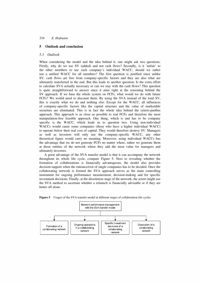
A great advantage of the SVA transfer model is that it can accompany the network throughout its whole life cycle, compare Figure 5. Next to revealing whether the formation of collaborations is financially advantageous, the model also provides decision-support when the entrance/exit of single companies has to be decided. Once the collaborating network is formed the SVA approach serves as the main controlling instrument for ongoing performance measurement, decision-making and for specific investment decisions. Finally, at the dissolution stage of the network, the actors might use the SVA method to ascertain whether a relaunch is financially advisable or if they are better off alone.

Figure 5 Usages of the SVA transfer model at different stages of collaboration life cycles


An important question is how the model deals with the common situation that a collaborating member is also a member of additional different networks at the same time. We can use the German company Bosch as an example, a key supplier of many automobile manufacturers throughout the whole world. Bosch is engaged in multiple supply chains that are even competing against one another. Generally, this is not a problem as long as the two supply chains’ goals are not interfering. Since we compare all potential network alternatives against the current state, our value-maximising strategy is unchanged: the largest overall SVA also entails the largest individual SVA by means of the transfer system. Problems arise if a company is member of two or more networks that are interdependent or even conflicting. A strategy or alternative that is value-adding for one network might be less valuable or even harmful for another. Consequently, the multi-engaged company is stuck in choosing between separate value-maximising strategies. It seems logical that the multi-engaged company will prefer the strategy that will maximise his individual SV. If this is a strategy to be realised by network A, network B might not realise its optimal strategy, as illustrated by Figure 6, for example, if the issue is about a building of a new logistics warehouse for the multi-engaged company. For network A, it might be optimal to build this warehouse at another spot than would be optimal for network B. To build an extra warehouse for each collaborating network would make no sense for the multi-engaged company. Consequently, the optimal strategies for network A and B are mutually exclusive, for example, both networks are thinking about building a logistics warehouse to be managed by the double-engaged company. For network A it is better to build this warehouse at Location 2 while network B is better of if the warehouse is built at Location 1. To build an extra warehouse for each network would not be smart for the multi-engaged company due to economies of scale. Consequently, the optimal strategies for network A and B are mutually exclusive and conflicting. Unless network B can come up with an alternative where the company with double-involvement is better off, there is no incentive for the company to participate in network B’s solution. From network B’s point of view, the EUR 2,500,000 to be realised by the company when choosing Alternative 2 therefore represent the company’s Threshold-SVA. The problem could be solved financially by giving additional payments to the company. But in fact, the problem is more complex: next to financial issues, the whole relationship of trust and joint efforts is at stake. By choosing the value-maximising strategy with network A, the company might put its relations to network B at risk. It therefore seems more advisable to bring both networks to one table and collectively find a solution that is acceptable for both.

Figure 6 Example for conflicting strategies between two inter-related networks

336 E. Hofmann

5.2 Conclusions

In today’s turbulent, fast paced business environment, it is difficult for companies to establish a sustainable source of competitive advantage. Collaborating networks offer a promising vehicle for overcoming this problem. In recent years, much has been written about the merits of collaborating networks. However, this paper contends that companies will fail to reap the potential rewards of collaborating unless they redefine how they measure and reward network performance. The newly developed SVA transfer model is a performance measurement tool that can be used to help align the incentives of network partners and achieve financial prosperity. We believe that this is one of the first paper to explicitly combine issues that have been separately considered in the network/ supply chain management and VBM literature. It broadens both the literature schools by studying ‘quantitative’ performance measurement opportunities in network environments. Further, it provides practical insights into the network performance management and gives executives evidences to gain the merits of network approaches like the supply chain management concept.

References

Baiman, S., Fischer, P.E. and Rajan, M.V. (2001) ‘Performance measurement and design in supply chains’, Management Science, Vol. 47, No. 1, pp.173–188.

Ballou, R.H., Gilbert, S.M. and Mukherjee, A. (2000) ‘New managerial challenges from supply chain opportunities’, Industrial Marketing Management, Vol. 29, No. 1, pp.7–18.

Beamon, B.M. (1999) ‘Measuring supply chain performance’, International Journal of Operations and Production Management, Vol. 19, No. 3, pp.275–292.

Berman, S.L., Wicks, A.C., Kotha, S. and Jones, T.M. (1999) ‘Does stakeholder orientation matter? The relationship between stakeholder management models and firm financial performance’, Academy of Management Journal, Vol. 42, No. 5, pp.488–506.

Booth, L. (1998) ‘What drives shareholder value? Paper Presented at the Federated Press ‘Creating Shareholder Value’ Conference, 28 October 1998, University of Toronto, Toronto.

Bowersox, D.J., Closs, D.J. and Keller, S.B. (2000) ‘How supply chain competency leads to business success’, Supply Chain Management Review, Vol. 4, No. 4, pp.70–78.

Brealey, R.A. and Myers, S.C. (2000) Principles of Corporate Finance, 6th edition, Boston etc.

Casey, C. (2001) ‘Corporate valuation, capital structure and risk management: a stochastic DCF approach’, European Journal of Operational Research, Vol. 135, No. 2, pp.311–325.

Christopher, M. and Ryals, L. (1999) ‘Supply chain strategy: its impact on shareholder value’, The International Journal of Logistics Management, Vol. 10, No. 1, pp.1–10.

Coyle, B. (2000) Capital Structuring, Chicago, etc.

Deimel, K. (2002) ‘Shareholder value-konzept, capital asset pricing model und kapitalwertmethode’, Das Wirtschaftsstudium, Vol. 31, No. 1, pp.77–82.

Eccles, R.G. and Pyburn, P.J. (1992) ‘Creating a comprehensive system to measure performance’, Management Accounting, Vol. 74, No. 4, pp.41–44.

Emery, D.R. and Finnerty, J.D. (1991) Principles of Corporate Finance with Corporate Applications, St. Paul, etc.

European Logistics Association (ELA)/Bearing Point (2002) What Matters to Top Management? A Survey on the Influence of Supply Chain Management on Strategy and Finance, Brussels.

Farris, M.T. and Hutchison, P.D. (2003) ‘Measuring cash-to-cash performance’, The International Journal of Logistics Management, Vol. 14, No. 2, pp.83–91.


Gjerdrum, J., Shah, N. and Papageorgiou, L.G. (2002) ‘Fair transfer price and inventory holding policies in two-enterprise supply chains’, European Journal of Operational Research, Vol. 143, No. 3, pp.582–599.

Hertenstein, J.H. and McKinnon, S.M. (1997) ‘Solving the puzzle of the cash flow statement’, Business Horizons, Vol. 40, No. 1, pp.69–76.

Hieber, R. (2002) ‘Collaborative performance measurement in logistics networks – the model, approach and assigned KPIs’, Logistik Management, Vol. 4, No. 2, pp.25–33.

Hofmann, E. (2003) ‘The flow of financial resources in the supply chain: creating shareholder value through collaborative cash flow management’, in H. Kotzab (Ed). Eighth ELA Doctorate Workshop 2003, Brussels, pp.67–94.

Hofmann, E. (2005) ‘Supply chain finance: some conceptual insights’, in R. Lasch, and C.G. Janker (Eds). Logistik Management – Innovative Logistikkonzepte, Wiesbaden, pp.203–214.

Keown, A.J., Petty, J.W., Martin, J.D. and Scott, D.F. (2001) Foundations of Finance. The Logic and Practice of Financial Management, 3rd edition, New Jersey: Upper Saddle River.

Lalonde, B. (2000) ‘Making finance take notice’, Supply Chain Management Review, Vol. 4, No. 5, pp.11–12.

Lambert, D.M. and Pohlen, T.L. (2001) ‘Supply chain metrics’, The International Journal of Logistics Management, Vol. 12, No. 1, pp.1–19.

Lane, P.J., Canella, A.A. and Lubatkin, M.H. (1998) ‘Agency problems as antecedents to unrelated mergers and diversification: Amihud and Lev reconsidered’, Strategic Management Journal, Vol. 19, No. 6, pp.555–578.

McNann, P. and Nanni Jr, A.J. (1994) ‘Is your company really measuring performance?’ Management Accounting, Vol. 76, No. 5, pp.55–58.

Mills, R.W. and Chen, G. (1996) ‘Evaluating international joint ventures using strategic value analysis’, Long Range Planning, Vol. 29, No. 4, pp.552–561.

Neely, A., Gregory, M. and Platts, K. (1995) ‘Performance measurement system design’, International Journal of Operations and Production Management, Vol. 14, No. 4, pp.19–34.

Otto, A. and Kotzab, H. (2003) ‘Does supply chain management really pay? Six perspectives to measure the performance of managing a supply chain’, European Journal of Operational Research, Vol. 144, No. 2, pp.306–320.

Ramdas, K. and Spekman, R.E. (2000) ‘Chain or shackles? Understanding what drives supply-chain performance’, Interfaces, Vol. 30, No. 4, pp.3–21.

Rappaport, A. (1998) Creating Shareholder Value. A Guide for Managers and Investors, 2nd edition, New York.

Singhai, V.R. and Hendricks, K.B. (2002) ‘How supply chain glitches torpedo shareholder value’, Supply Chain Management Review, Vol. 6, No. 1, pp.18–24.

Srivastava, R., Shervani, T.A. and Fahey, L. (1998) ‘Market-based assets and shareholder value: a framework for analysis’, Journal of Marketing, Vol. 62, No. 1, pp.2–18.

Timme, S. and Williams-Timme, C. (2000) ‘The financial-SCM connection’, Supply Chain Management Review, Vol. 4, No. 2, pp.33–40.

Vitale, M.R. and Mavrinac, S.C. (1995) ‘How effective is your performance measurement system?’ Management Accounting, Vol. 77, No. 2, pp.43–47.

338 E. Hofmann

Appendix

Formula 1 (F1)

( )WACC= * * *+

where :

: Market value of equity

: Market value of debt

: Cash tax rate

: Cost of debt

: Cost of equity

E

D

E

Ei i

E D

E

D

r

i

i

+ −+ DD 1 r

E D

An introduction to the CAPM- and the WACC-approach can be obtained from any basic finance class book, for example, Emery and Finnerty (1991), Coyle (2000) or Brealey and Myers (2000).

Formula 2 (F2)

Sales

– Cost of goods sold (COGS)

– Selling, general and administration expenses

– Depreciation

– Other operating expenses

_________________________________________

= Earnings before interest and taxes (EBIT)

– Cash Taxes (pre interest)

+ Non-cash changes

_________________________________________

= Net operating profit after tax (NOPAT)

– Increase in non-cash NWC

– Incremental capital

(after tex)

expenditure

_________________________________________

= Free Cash Flow

Alternative derivations of the FCF can be found in Emery and Finnerty (1991), Keown et al. (2001) and Booth (1998).


Appendix (contined)

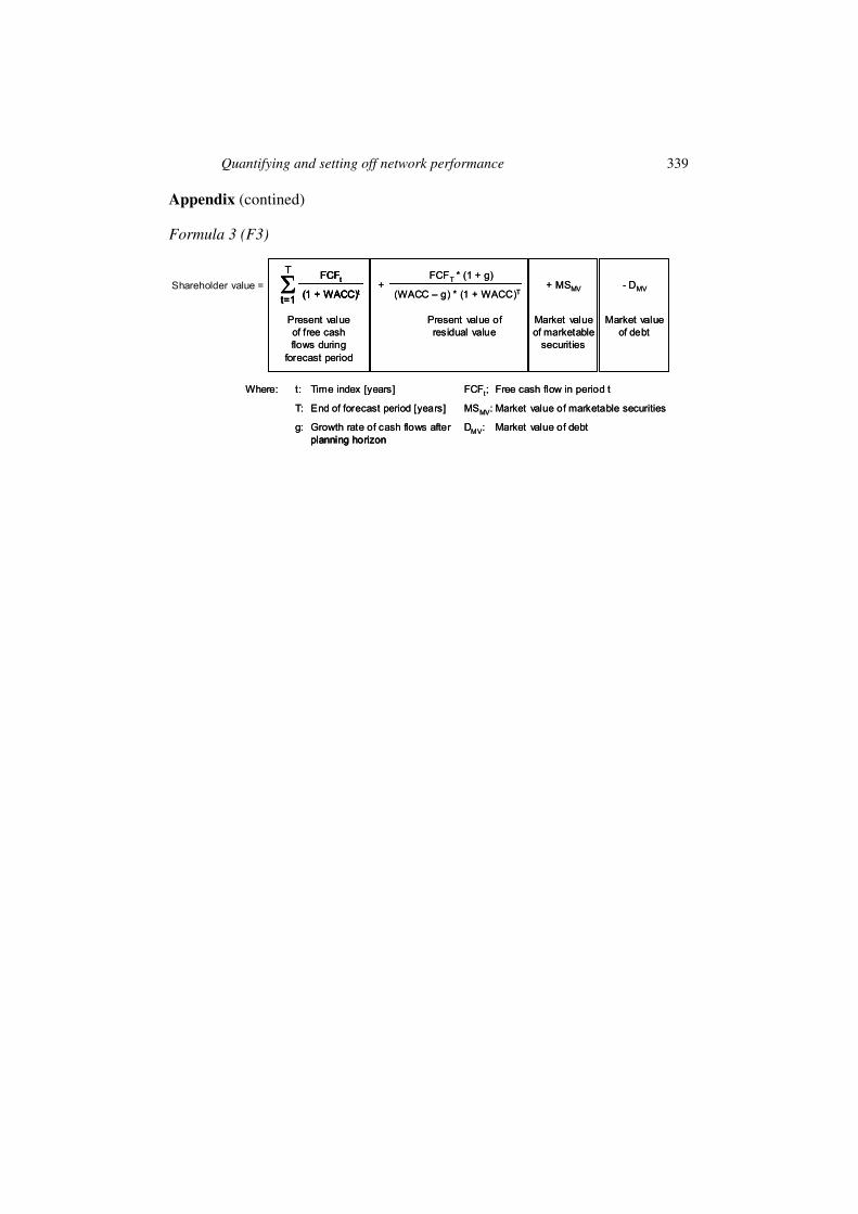
Formula 3 (F3)

Shareholder value =T

t=1Σ FCFt

(1 + WACC)t

Present value of free cash flows during

forecast period

FCFT * (1 + g)

(WACC – g) * (1 + WACC)T+

Present value of residual value

+ MSMV

Market value of marketable

securities

- DMV

Market value of debt

t: Time index [years]

T: End of forecast period [years]

g: Growth rate of cash flows after planning horizon

FCFt; Free cash flow in period t

MSMV: Market value of marketable securities

DMV: Market value of debt

Where:

Shareholder value =T

t=1Σ FCFt

(1 + WACC)t


forecast period

T

t=1Σ FCFt

(1 + WACC)t

T

t=1ΣT

t=1Σ FCFt

(1 + WACC)tFCFt

(1 + WACC)t


forecast period

FCFT * (1 + g)



FCFT * (1 + g)



+ MSMV


securities

+ MSMV


securities

- DMV


- DMV


t: Time index [years]






Where: t: Time index [years]






Where:

quantifying and setting off network performance network performance... · quantifying and setting...

Documents