quality competition in mobile telecommunications: …pks2120/sunpatrickjmp.pdfquality competition in...
TRANSCRIPT

Quality Competition in Mobile Telecommunications:
Evidence from Connecticut
Patrick Sun*
Columbia University
April 20, 2015
Job Market Paper
Abstract
Signal quality is a significant contributor to the overall quality of wireless telephone service,
which competitive analyses often overlook. To understand how further consolidation in this
industry would impact the competitive incentives for signal quality investment, I estimate de-
mand and supply of wireless service using a proprietary market research survey and a unique
Connecticut database of antenna facilities, or base stations. Dropped call rates and local cover-
age improve as base station density increases, so I treat base station density as an endogenous
product characteristic and relate it to the local value of wireless service. On average, I find a 1%
increase in log base station density results in a market share gain of 0.17% to the investing firm
and a loss of 0.04% for each rival. Base station costs are implied to be substantial, so if these
costs can be effectively reduced through network integration after a merger, the merging firms
and consumers can both benefit through increased base station provision. If such integration
is not possible, consumers lose due to either a loss in variety of products or reduced incentives
of merged firms to provide quality. These results suggest that merger review must pay careful
attention to the potential for network integration in wireless and related industries.
JEL Classification: L15, L40, L96
Keywords: quality competition, merger analysis, telecommunications.
*Columbia University (email:[email protected]). Please visit http://www.columbia.edu/~pks2120/
research.html for the latest draft. I would like to thank my adviser Michael Riordan, Kate Ho, Chris Conlon,Christophe Rothe, Bernard Salanie, Colin Hottman, Keshav Dogra, Michael Mueller-Smith, Christopher Mueller-Smith, Ilton Soares, Alejo Czerwonko, Donald Ngwe, Hyelim Son, Ju-Hyun Kim, Jonathan Dingel, and all attendeesof the Columbia Industrial Organization Colloquium. I gratefully acknowledge the financial support of this researchby the NET Institute, http://www.NETinst.org. I would also like to thank the various wireless industry experts whotook the time to educate me on the details of this industry. All errors are mine.

1 Introduction
The wireless industry is an important part of the U.S. economy, with $189 billion dollars of revenue
in 2013.1 Not only does wireless service provide significant benefits to society from direct consump-
tion, but also it improves the productivity of other economic activities.2 Of the many aspects of
the quality of wireless service, the quality of the signal - the ability to make, receive and maintain
calls - seems to be especially important. In a market research survey in 2008, consumers most fre-
quently reported “Better Coverage” (21%) above “Lower Prices” (19%) as the reason for choosing
their carrier.3 The firms in this industry, also called “carriers”, seem to care about improving their
quality they invest heavily in capital, spending $ 33 billion in 2013 alone.4
An important part of this investment are the antennas and supporting equipment that have to
be built and maintained in local market areas. As these facilities, or base stations, become more
common in an area, the signal quality improves as the average distance between consumers and
the antennas decreases. A carrier can increase its market share by building more base stations in a
local market, but base stations are costly in terms of materials, power, maintenance and regulatory
compliance. Carriers must build their own base stations to serve their customers, so base station
investment is a competitive activity.5 Unlike price, quality improvements in one firm may not
induce other firms to improve quality in kind to compete - rather they may be discouraged from
competing directly with the now stronger rival and reduce their quality response. Thus a natural
question is how competition affects the incentive to provide signal quality in this economically
important industry.
This question is especially relevant in the U.S., where the four nationally available carriers,
AT&T, Sprint, Verizon and T-Mobile, have approximately 93% national market share.6 It is not
clear at this high concentration whether the carriers exert competitive pressure on each other to
provide quality, and if so, how great that pressure is. Moreover, the industry appears eager to
1From “CTIA-The Wireless Association, CTIA’s Wireless Industry Summary Report, Year-End 2013 Results,2014.” See http://www.ctia.org/your-wireless-life/how-wireless-works/annual-wireless-industry-survey.
2A literature, surveyed by Aker and Mbiti (2010), show how wireless telephones have significantly reduced infor-mation frictions in markets in developing countries. Roller and Waverman (2001) gives evidence on the impact oftelecommunications infrastructure on aggregate productivity.
3See Table 1.4From “CTIA-The Wireless Association, CTIA’s Wireless Industry Summary Report, Year-End 2013 Results,
2014.” See http://www.ctia.org/your-wireless-life/how-wireless-works/annual-wireless-industry-survey.5Carriers occasionally share a single base stations in extraordinary situations.6See “6 years after the iPhone launched, just 4 big carriers are left standing”,
http://venturebeat.com/2013/07/08/iphone-carrier-consolidation/, July 8, 2013.
1

undergo further consolidation. AT&T attempted to merge with T-Mobile in 2011 before facing
opposition from antitrust authorities later in the year. T-Mobile merged with the fifth largest
carrier MetroPCS in 2013. During the middle of 2014, Sprint and T-Mobile discussed merging,
but called off the effort due to expected antitrust opposition (allegedly).7 Since signal quality
readjustments might counteract or reinforce negative price effects from a merger, the merger effect
on incentives to provide signal quality has important policy implications.
Competitive analyses, both in antitrust practice and the academic literature, generally focus
on price changes from market structure changes, holding all other quality dimensions fixed. In
contrast, I conduct an analysis treating signal quality as an endogenous variable under the control
of firms. Consumer utility for a given carrier’s network is modeled as a function of the density of
that carrier’s base stations. I estimate this model using two unique datasets for Connecticut where
I directly observe base station location and ownership and consumer carrier choices in the state
from 2008-2012. I combine my demand estimates with a model of quality competition to recover
the costs of maintaining base stations. I then use the parameter estimates and full model to run
counterfactual simulations of the proposed AT&T and Sprint acquisitions of T-Mobile.
Across carriers, markets and years, I find that a 1% increase in the observed level of log base
station density results in a median market share gain of 0.17% for the investing firm, and median
losses of 0.04% for each rival firm. These small effects are not unexpected since a firm invests in
bases station until the return for the marginal base station is low. Accordingly, implied expenditures
on all base stations, including the inframarginal ones, are substantial. For example, T-Mobile is
estimated to spend about 60% of variable profits on its base stations.
Further, the demand estimates and model of competition end up implying that base stations
are locally a strategic substitute, in the sense of Bulow, Geanakoplos, and Klemperer (1985): rival
increases in base stations reduce the incentives to provide own-base stations. Mergers may cause
firms to adjust base stations in one direction, but that will in turn cause rival firms to adjust base
stations in the opposite direction. Thus the overall sign of welfare effects is ambiguous without
accurate parameter estimates.
Simulation of mergers between a “small” carrier (T-Mobile) and two of its major rivals (AT&T
and Sprint) suggest that the scope for integration of the two merging firms’ networks is crucial
7“Sprint Abandons Pursuit of T-Mobile, Replaces CEO”, Wall Street Journal, August 5, 2014.
2

for consumer-welfare improving conduct. Eliminating the acquired carrier and its network entirely
results in the remaining firms increasing quality due to strategic substitutability, but not enough
to make up for the consumer welfare loss from the decrease in variety. Keeping the acquired
product line around instead but also keeping the networks separate results in a decrease in signal
quality by the two merged firms since now they internalize the negative impact each network has
on the others’ product lines. Only in the counterfactuals where the consumers can use their phone
on both networks are consumer gains realized. A base station can serve consumers who have a
horizontal taste for either product line of the merging firms, whereas before they could only serve
one or the other. This spillover across product lines makes marginal investments in base stations
more effective in terms of attracting consumers. This translates into a greater incentive to provide
quality relative to its cost. Under reasonable assumptions about prices and costs, consumers benefit
as effective quality improves even if the total number of base stations decreases. These effects are
qualitatively similar whether the acquiring firm is the AT&T or Sprint, though the negative impacts
of mergers are blunted somewhat when the acquirer is the smaller Sprint. Thus from the perspective
of competitive and telecommunication policy, merger reviews in the wireless and other network-
based industries should require detailed evidence from applicants about the potential and plans for
network integration.
This study contributes to the literature on merger evaluation which has long history in eco-
nomics. Works such as Salant, Switzer, and Reynolds (1983), Perry and Porter (1985), Deneckere
and Davidson (1985) and Farrell and Shapiro (1990) examined equilibrium welfare effects of merg-
ers and showed that they depended on more than simply industry concentration. Given these
ambiguous effects, later economists began to use new empirical techniques to estimate the poten-
tial effects of mergers. Early examples, like Werden and Froeb (1994), Nevo (2000), and Town and
Vistnes (2001), focused on price effects as the theory literature had, but later works, like Draganska,
Mazzeo, and Seim (2009) and Fan (2013) also looked at the effect of other product characteristics.
This paper belongs to the latter literature and uses base station density as an endogenous non-price
characteristic to apply this methodology to a large and economically significant industry. Like those
papers, this means the analysis also belongs to the discrete choice demand estimation literature
which controls for endogenous product characteristics, such as Berry (1994) and Berry, Levinsohn,
and Pakes (1995).
3

This study also contributes to the literature on the economics of wireless service. Among the
earliest studies is Hausman (1999), which attempts to quantify the bias in the US CPI from the
exclusion of the mobile phones from the index. Busse (2000) and Miravete and Roller (2004) study
the early U.S. industry in which the U.S. Federal Communications Commission (FCC) restricted
each market to a duopoly. As the carrier-customer relationship is often mediated by contract, there
is some recent literature using wireless phone data to test contract theory (See Luo (2011), Luo
(2012), Luo, Perrigne, and Vuong (2011)). The long-term contracting environment also provides a
laboratory for studying dynamic optimization. For example, Yao, Mela, Chiang, and Chen (2012)
use mobile phone contracts to estimate discount rates, while Jiang (2013) and Grubb and Osburne
(Forthcoming) show errors in dynamic optimization of minutes usage.
Another part of the wireless literature, to which this paper belongs, uses discrete choice demand
systems to estimate wireless operator incentives. Often these papers include signal quality as a
component of consumer utility, but only as a exogenous control. For example, Zhu, Liu, and
Chintagunta (2011) and Sinkinson (2014) both study the value of the exclusivity of the iPhone to
AT&T and include measures of signal quality. Similarly, Macher, Mayo, Ukhaneva, and Woroch
(2012) study the substitution and complementarity of fixed and wireless lines, and include the
total number of national number of cell sites, locations that house base stations, in their demand
system to proxy for improving quality of cell service overall. The aforementioned Miravete and
Roller (2004) also includes cell sites in their analysis, though they do not include it as a quality
proxy. Rather, they use it to proxy demand since they assume each site serves some fixed number
of customers.
My paper is distinguished from the above as its focus is the carriers’ incentives to change signal
quality so signal quality cannot be assumed exogenous. In this respect, the most similar paper in
the literature to mine is Bjorkegren (2013), who looks at the Rwandan quasi-monopoly to estimate
positive demand externalities consumers have on each other in wireless. As he has access to the
Rwandan operator’s private data, he also has information about base station location and includes
coverage as an endogenous component of utility. Given the complexities of his model, he cannot
fully simulate equilibrium coverage provision even for the monopoly, but does partial equilibrium
counterfactuals about base station location in response to a government program.8 In contrast
8Specifically, Bjorkegren removes the 10 base stations with the lowest revenues to simulate a policy imperative forthe quasi-monopoly serve rural areas and then sees how demand responds.
4

to Bjorkegren (2013), my model is greatly simplified, but provides a unified framework for policy
experiments taking into account the strategic aspect of quality decisions.
In the remaining sections of this paper, I illustrate how I implement this framework. I explain
the industry, how my model captures the aspects of this industry relevant to signal quality provi-
sion, and the results from estimation of that model. I then implement a variety of counterfactual
simulations using my results to explore mergers in this industry and then conclude with an overview
of the findings. However, since the incentives behind signal quality provision may not be obvious,
I start with a simple example model to illustrate the intuition.
2 Competitive Effects of Quality
The welfare effects from a market structure change are largely determined by whether quality is
a strategic complement or a strategic substitute, as defined by Bulow, Geanakoplos, and
Klemperer (1985).
In a game, strategic complements are a set of control variables for the players such that if a
change in one player’s variable induces rivals to change their variable in the same direction. For
example, price is a strategic complement in Bertrand competition. In that game, the downside
of cutting price is that while lower prices brings new consumers, old consumers who would have
bought at the original price are now given a discount. If a rival decreases price, there are fewer old
consumers so the gross loss via the discount to these consumers is smaller and price cutting is less
costly.
Analogously, strategic substitutes are control variables that when changed induce changes of
rivals in the opposite direction. Quantity in Cournot competition is a strategic substitute. If a
rival expands their demand, then the market price goes down. Thus own demand expansion is less
beneficial since there is less revenue per consumer.
If quality is a strategic complement, signing the welfare effect of a merger is straightforward,
since the effect the merger has on the quality of the merging firms would be reinforced by like
quality changes of the non-merging firms. Strategic complements thus simplifies antitrust analysis
with regards to price which is generally a strategic complement: a merger that would induce price
increases holding non-merging firm’s prices fixed must be anticompetitive since full equilibrium
would only imply more price increases by rivals. But quality could be a strategic substitute,
5
then the sign of the welfare effect of the merger is ambiguous, since any effect on the quality of
the merging firms might be completely canceled out by the changes of the non-merging firms.
Therefore, analysis of mergers taking endogenous quality into account needs to determine both
whether the merger will induce merging parties to change quality and the direction of the response
of non-merging rivals.
In the model I take to the data, it turns out that strategic complementarity and substitutability
depend on the shape of the demand function and where the relative utilities of the plans put the
different carriers on that demand function. To illustrate the forces at work in the estimated model,
consider the following simple example model. Let there be two carriers, indicated by k ∈ 1, 2. Each
offers a single product. In a first stage, the carriers set national prices. In the second stage, they
set local signal quality Qk by adjusting the number of their base stations. Consumers choose the
carrier which gives them the most utility or an outside option k = 0. Utility of the two products
are
Uik = Qk + εik (1)
εik is a mean-zero random shock, which is independently and identically distributed over ik and
explains why all consumer do not just choose the carrier with highest mean quality. For simplicity,
I normalize the outside option to always have utility 0.
The market share is determined by a function Sk(Q1, Q2) of the signal quality. Assuming a
market population and constant markups normalized to 1 and cost function φ(Qk), profit is
πk = Sk(Q1, Q2)− φ(Qk) (2)
Taking Qk as continuous and φ(Qk) as sufficiently convex, then a pure strategy Nash equilibrium
exists and the necessary first order condition is:
dπkdQk
=∂Sk(Q1, Q2)
∂Qk− ∂φ(Qk)
∂Qk(3)
i.e. marginal variable profit for quality equals marginal quality cost.
Invoking Topkis (1978) and Milgrom and Shannon (1994), the comparative statics depend on
6

the sign of this cross partial derivative of profit since the control variables are assumed continuous.
The cross partial of the example profit function of k with respect to rival quality h depends entirely
on the share/demand function, since rival signal quality does not enter the cost function.9 Thus
the pivotal factor in determining strategic substitutes or complements will be how a change in rival
quality affects the number of marginal consumers from a quality increase. If the marginal consumers
increase in number, then quality is a strategic complement, if marginal consumers decrease, then
strategic substitutes.
What makes a consumer marginal for 1? A consumer must be indifferent between 1 and 2 or the
outside option, which implies she must get certain levels of shocks such she have the same utility
for 1 as 2 or the outside option. Denote the identical CDFs of these errors as G and their PDFs as
g.
Consumer i chooses good 1 if Q1 + εi1 > 0 and Q1 + εi1 > Q2 + εi2. If Q2 + εi2 < 0↔ εi2 < −Q2
then the outside option utility is always greater than that of good 2. Demand is then equal to how
often the utility of good 1 is greater than the utility of the outside option - the probability that
Q1 + εi1 > 0 ↔ εi1 > −Q1. Analogously, if Q2 + εi2 < 0 ↔ εi2 < −Q2 then the good 2 utility is
always greater than that of the outside option. Demand is then equal to how often the utility of good
1 is greater than the utility of good 2 - the probability that Q1+εi1 < Q2+εi2 ↔ εi1 < Q2−Q1+εi2.
Demand of good 1 is therefore expressible as the following integral over the distribution of the
normalized errors:
S1(Q1, Q2) =
∫ −Q2
−∞(1−G(Q1|εi2))g(εi2)dεi2 +
∫ +∞
−Q2
(1−G(Q2 −Q1 + εi2|εi2))g(εi2)dεi2 (4)
An infinitesimal change in Q2 has an infinitesimal impact on the demand of good 1 when good
2 is the worse than the outside option since all substitution happens between 1 and 0 there. The
only effect is to infinitesimally reduce the support on which this is the case. So Q2 has effectively
no impact on marginal return from that first part of the equation.
9Note that with a different cost function, this implication might change. For example, Chu (2010) studies qualityprovision in the form of channels offered by cable companies. In his case, quality costs do not enter separately fromdemand, since channel contracts payments are per subscriber. Thus it is possible in that setting, even without theheterogeneity he includes in his specification, to have entry of satellite competition or rival improvements in qualityinduce own quality improvements since the resulting loss of demand reduces marginal consumer costs. In the wirelessindustry, marginal consumer costs should, if anything, go down with more own base stations, since it might be lesscostly to maintain calls with a smaller territory associated with each base station. That assumption would implystrategic substitutability of base stations even more strongly, since now entry or rival quality improvement decreasesown demand and thus decreases total cost per marginal consumer.
7

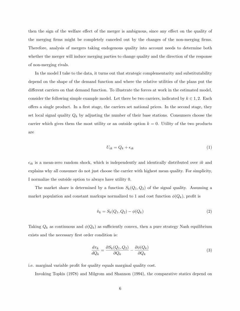
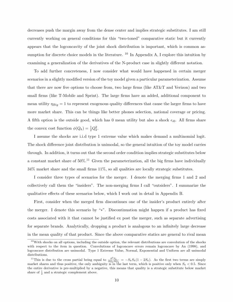
Figure 1: The lines separate the distribution of consumers, represented by the shading, into those whobuy Product 1, 2 and the Outside Option 0. The origin is set to (−Q2,−Q1). The Green line representsconsumers indifferent between 1 and 0, the Blue between 0 and 2, and the Red between 1 and 2. The shift inlines represents a change in the quality of 2.
∆Q20 2
1
εi1
εi2
(a) Q1 is a strategic substitute for Q2
∆Q20 2
1
εi1
εi2
(b) Q1 is a strategic complement for Q2
Thus the entire effect in the cross partial will be on the range where good 2 is better than
the outside option, i.e. where consumers are substituting directly between between 1 and 2. The
resulting cross partial is:
∂2S1
∂Q1∂Q2=
∫ +∞
−Q2
g′(Q2 −Q1 + εi2|εi2)g(εi2)dεi2 (5)
This expression makes sense - the overall cross partial is the conditional expected value of how fast
the density of marginal consumer between 1 and 2 grows as the the relative quality of the rival
good 2 grows. If greater rival relative quality increases the number of marginal consumers, then
the PDF grows, and quality must be a strategic complement. Analogously, if greater rival relative
quality reduces the number of marginal consumers, quality is a strategic substitute.
Figure 1 diagrams the example model in two different cases. Here I represent the distribution
of consumers by plotting the ε1 and ε2 space and shade the background of the graph to represent
denser parts of the space. I assume the shocks are unimodal, which is equivalent to assuming
consumers are less common the more extreme their predisposition to either goods 1 and 2 . The
carriers and outside option split the space of consumers: the outside option taking anyone who
does not have at least shocks greater than −Q1 and −Q2; 1 taking remaining consumers with high
εi1 and low εi2; and 2 taking remaining consumers with high εi2 and low εi1.
The Red line represents consumers indifferent between 1 and 2, the Green indifferent between
1 and the outside option, and the Blue the indifferent between 2 and the outside option. The
8

marginal incentives to invest are represented by the density of marginal consumers who would
switch between firms by an infinitesimal quality increase. For 1, this is equal to the consumers
along the Green and Red lines, and for 2, the Blue and Red lines.
The diagram shows the effect on those lines after an increase in Q2. There are fewer consumers
who are indifferent between 0 and 1 since some now prefer 2, so the green line gets shorter, but
while this looks substantial in the diagram, as explained earlier with infinitesimal rival quality
changes this effect also becomes infinitesimal. The first order change is that Red line gets shifted
left, meaning that the consumers who substitute between 1 and 2 must be more biased in terms of
shocks relative to 1. In left subfigure, one can see that the shift moves the Red line into a less dense
region of the graph, so the Red line must contain fewer consumers. Thus the Q2 increase decreases
marginal consumers, so quality a strategic substitute for the example drawn above. The marginal
consumer between 1 and 2 must now be more predisposed to 1, but this means that consumer is
less common.
However, this doesn’t mean quality is a strategic substitute for all quality levels. If the starting
points of the lines were else in the graph, say more to the right as in the right subfigure, then
the same shift would result in the Red line going from a region of few consumers to the center
region with more consumers. Then quality is a strategic complement as the Red line, the marginal
consumers between 1 and 2, has more density. This corresponds to the case where the qualities
are not similar: Q1 is much higher than Q2, so 1 has high market share and has captured most
of the market. The marginal consumers for 1 are thus people who are actually very predisposed
not to buy 1, so they are few in number. When Q2 increases, 2 is a better product and thus those
consumers will switch to 2. The marginal consumers between 1 and 2 are thus now less predisposed
to 2, and are thus more numerous.
Given unimodal shocks in each dimension, a general intuition for N-products is suggested. De-
pending on the exact shape of the distribution and holding other qualities fixed, there is some level
of Qk1 where above Q1 is a strategic substitute for a given Qk, and below is a strategic substitute.
When a product has far superior quality relative to the other option, then quality is strategic
complement because the relevant are margins are in the decreasing parts of the multidimension
“hump”. Relative quality decreases brings the margin back to the dense center and implies strate-
gic complements. Otherwise, the margin is in the increasing part of the hump, and relative quality
9
decreases push the margin away from the dense center and implies strategic substitutes. I am still
currently working on general conditions for this “two-toned” comparative static but it currently
appears that the logconcavity of the joint shock distribution is important, which is common as-
sumption for discrete choice models in the literature. 10 In Appendix A, I explore this intuition by
examining a generalization of the derivatives of the N-product case in slightly different notation.
To add further concreteness, I now consider what would have happened in certain merger
scenarios in a slightly modified version of the toy model given a particular parameterization. Assume
that there are now five options to choose from, two large firms (like AT&T and Verizon) and two
small firms (like T-Mobile and Sprint). The large firms have an added, additional component to
mean utility ηBig = 1 to represent exogenous quality differences that cause the larger firms to have
more market share. This can be things like better phones selection, national coverage or pricing.
A fifth option is the outside good, which has 0 mean utility but also a shock εi0. All firms share
the convex cost function φ(Qk) = 12Q
2k.
I assume the shocks are i.i.d type 1 extreme value which makes demand a multinomial logit.
The shock difference joint distribution is unimodal, so the general intuition of the toy model carries
through. In addition, it turns out that the second order condition implies strategic substitutes below
a constant market share of 50%.11 Given the parameterization, all the big firms have individually
34% market share and the small firms 11%, so all qualities are locally strategic substitutes.
I consider three types of scenarios for the merger. I denote the merging firms 1 and 2 and
collectively call them the “insiders”. The non-merging firms I call “outsiders”. I summarize the
qualitative effects of these scenarios below, which I work out in detail in Appendix B.
First, consider when the merged firm discontinues one of the insider’s product entirely after
the merger. I denote this scenario by “∗”. Discontinuation might happen if a product has fixed
costs associated with it that cannot be justified ex post the merger, such as separate advertising
for separate brands. Analytically, dropping a product is analogous to an infinitely large decrease
in the mean quality of that product. Since the above comparative statics are general to rival mean
10With shocks on all options, including the outside option, the relevant distributions are convolution of the shockswith respect to the item in question. Convolutions of logconcave errors remain logconcave by An (1998), andlogconcave distribution are unimodal. Type 1 Extreme Value, Normal, Exponential and Uniform are all unimodaldistributions.
11This is due to the cross partial being equal to ∂2Sk∂Qk∂Qh
= −SkSh(1 − 2Sk). As the first two terms are simplymarket shares and thus positive, the only ambiguity is in the last term, which is positive only when Sk < 0.5. Sincethe entire derivative is pre-multiplied by a negative, this means that quality is a strategic substitute below marketshare of 1
2and a strategic complement above.
10
quality in general and not just signal quality, there is a strong incentive to increase signal quality
by all remaining firms.
Next, consider when the insiders keep all their products and nothing else changes except for the
joint control. Denote this scenario and the joint firm as “∗∗”. Joint control causes the insiders to
not only care about how much improvements in quality of 1 increases demand for 1, but also how
it steals demand from product 2, and vice versa. Thus incentive for quality provision decreases for
both insiders, which in turn leads to higher incentives to provide quality for outsiders due to the
strategic substitution. One can also show that strategic substitutes are stronger for the insiders,
so it could be the case that quality level of one of the insiders increases in equilibrium because the
incentive to decrease the other insider’s quality is so strong.
Finally, consider when in addition to joint control, there are efficiencies from the merger in the
form of network integration. That is, if a consumer chooses carrier 1, that consumer can use 100%
of the quality of 1’s network, but also some fraction ρ of 2’s network quality. Denote this case
and the merged firm by ∗ ∗ ∗. For simplicity, I only consider the case of 100% spillover, ρ = 1,
but in principle one could argue it could be less due to incompatibility of handsets with some base
stations equipment, since installed technology varies from base station to base station, and from
firm to firm.12 The spillover makes each base station effectively cheaper, since each base station
can now serve multiple product lines. These are more consumers than would be served by a single
product line with equal amount of quality since the multiple brands capture consumer with different
horizontal tastes. This effective lower cost counteracts the lower incentives for quality provision
from the internalization carried over from scenario ∗∗, so overall incentives for quality provision are
higher relative to scenario ∗∗. Because of the strategic substitutability, the outsiders will have an
incentive to lower their quality. The spillovers also happen to increase the strategic substitutability
of insiders even relative to Scenario ∗∗, because now the firms have to consider how rival quality
effects the size of the spillovers. Thus the equilibrium result is even more ambiguous than Scenario
∗∗.
Table 2 shows the distribution of network quality and the consumer welfare impact in under
the above merger scenarios. I also report permutations with the size of the insiders for a total of
8 counterfactuals. As shown in McFadden (1978) and Small and Rosen (1981), expected welfare
12ρ = 0 is simply Scenario ∗∗.
11
for a consumer in the logit model is the log of the sum of the exponents of mean utility of all the
products available:
ln(1 +∑k∈K
exp(δk)) (6)
In general, when a carrier is lost completely, welfare decreases even when network quality of
all the remaining firms increases since due to loss of variety built into the logit. Even keeping the
products, if there is no network integration, consumers will be worse off as the internalization of
the cannibalization effects causes network quality losses that exceed compensating investment by
rival firms. When there is 100% spillovers, the result is markedly better for consumers as merging
firms increase joint network quality significantly relative when there are no spillovers. However, the
benefit depends on whether a merging firm is large or not - smaller firms merging is less harmful
since smaller firms contribute less to expected consumer welfare and have smaller cannibalization
effects. When a big firm is involved, these effects are much stronger, so that if the two large firms
merge the resulting joint firm reduces its network quality on net since the cannibalization effects
are so large. In summary, the only cases with net benefits to consumers the mergers with spillovers
and involving the small carriers.
The above results are only here to illustrate the range of possible outcomes and are based on
a particular set of parameters. Of the various forces at work, the one that wins out in equilibrium
depends on the true parameters. Moreover, while the assumption of unimodal shocks and the com-
parative statics they lead to seem reasonable, they are fairly restrictive. The results illustrated in
Figure 1 depend on the unimodal distribution that is dense in the middle of the error space. Given
an arbitrary multimodal distribution of consumers, there would be no strong prediction about the
strategic complementarity or substitution of quality. Thus, accurately assessing the merger welfare
implications of network quality in the mobile phone industry requires accurate estimation of param-
eters and a flexible demand system that admits potentially multi-modal consumer heterogeneity. I
explain how I do this in the context of the cell phone industry in the following sections.
12

3 Industry Background
To understand how I will model signal quality in context of the economic model requires some
background on both how the market for cellular service works in the U.S. and the technical aspects
on how that service is provided.
In the United States, consumers purchase a plan from carriers to provide service on their wireless
phones, or handsets. There are two kinds of plans, prepaid and postpaid. Prepaid plans are paid by
the minutes used, day or month (or by megabyte in data usage). They are called “prepaid” since
often one buys a card of fixed value that has to be replaced once depleted. In contrast, postpaid
plans are structured as a three-part tariff: there is a fixed monthly fee, but if a certain amount of
minutes or data is exceeded, the “overage” results in extra charges.13 Since the bills come at the
end of the usage period, the plan is “postpaid.” In the United States, postpaid plans dominate,
which is generally attributed to the “phone subsidy”: postpaid plans will give a discount on a
bundled handset, which the prepaid plan does not. U.S. postpaid plans generally take the form
of two-year contracts, which require an early termination fee to break. The postpaid plan also
requires a credit check that many low-income consumers cannot pass.
The handset is essentially a hand-held radio transceiver. When a call is made, the handset sends
information to the nearest antenna that services your carrier over that carrier’s frequency band of
the electromagnetic spectrum. These antennas are part of the carrier’s base stations, equipment
facilities that reroutes the information through the landline telephone system. If the receiver of the
call is also on a cell phone, the call will leave the landline network and be rerouted to the nearest
base station to the receiver, and the base station will beam the call information to the target.
Thus signal quality depends crucially on the ability of the base stations to form and maintain
transmissions. The power of the transmission decreases with distance, so if no carrier base station
is in range, then the signal power between the phone the base station will be too weak to start
a call. Even when a consumer is close enough to a base station to initiate a call, there can still
be problems since random ambient interference might overwhelm the signal and disrupt it. This
disruption ends the transmission of information, creating a “dropped call”.
Accordingly, carriers are interested in building base stations to make sure their market areas
13Note that this is not a two-part tariff, since in addition to the lump-sum subscription price there are two differentmarginal prices-below the overage limit, the marginal price zero, and over the limit the marginal price is positive.
13

are well covered and dropped calls are kept to a minimum. The more base stations in an area, the
more likely a consumer will be in range and the less likely a call would be dropped. I assume that
even if consumers do not know exactly where the base stations are, they do know the actual signal
quality from word of mouth, the internet and firm advertising.14
However, base stations are very costly. Aside from the costs of equipment, maintenance and
power, base stations must be mounted on elevated structures. Therefore, a large tower must be
built or space on a preexisting tall structure must rented. Developing and acquiring these locations,
or “sites”, requires significant regulatory proceedings with local zoning authorities, which can take
years. 15 Thus carriers face a trade-off between improving quality relative to their competitors and
paying high investment costs.
The value of each base station is likely to vary by firm, as signal quality depends also on
the technology and spectrum available to different firms. In the United States, different firms
use different technologies to encode their signals. AT&T and T-Mobile use variants of the GSM
standard, in which each call is apportioned a different part of the carriers spectrum in that area.
CDMA, used by Verizon and Sprint, interweave calls from all users over the carrier’s entire local
spectrum. Theoretically, a CDMA signal will travel farther than a GSM signal so a CDMA carrier
might need less base station density to yield more quality.
In addition, spectrum holdings is also a signal quality concern in two dimensions. First, spec-
trum represents the amount capacity of information that a base station can support in an area at
any one time. A call can be dropped or switched to another base station if spectrum becomes full
so a carrier with more spectrum may have less dropped calls. This concern seems minimal though
as industry sources I have spoken with characterize dropped calls due to capacity constraints as
only 5% of all dropped calls, and dropped calls are themselves around only 1-2% of calls in general.
Capacity is more of an issue when dealing with data, in which firms slow down data transfer to
deal with congestion. For the purposes of this analysis, I will abstract from capacity concerns
and assume firms have invested appropriately in upgrading their base stations to mitigate capacity
14There are various websites where individuals can post ratings of their quality levels, such cellreception.com andsignalmap.com. More recent sites such as opensignal.com use readings directly from phones using a mobile phone app.Unfortunately data from these sites either could not be scraped or turned out to be too thin for useful analysis. Forexample, cellreception.com only had about 400 ratings in total for the whole of Connecticut for the period between2003 and 2013.
15Such delays became so long that the FCC decreed a maximum delay time for responses to carrier inquiries aboutsite development. Objections from towns resulted in a 2012 Supreme Court Case: “City of Arlington, Texas, et al.v. FCC et al.”
14

issues over our sample period.16 This approach is in line with news reports, which characterizes a
spectrum shortage as a looming crisis, but noted that the U.S. had “slight spectrum surplus” as
of 2012. Given the limited amount of spectrum though and increasing use of data, capacity may
become a serious concern in the future.17
Second, and potentially more important, different parts of the electromagnetic spectrum have
different properties. Frequencies under 1000 MHz propagate farther and therefore are more useful
in rural areas. AT&T and Verizon have almost all this spectrum, since this was the first spectrum
apportioned to firms. Other current carrier like Sprint and T-Mobile are descendants of entrants
from the mid to late 1990s when most of the low frequency spectrum had already been distributed.
Thus, Sprint and T-Mobile might yield less quality from base stations than their rivals.18
In addition to varying across carriers, base station effectiveness will likely vary by markets due
idiosyncratic engineering aspects of the different locations. Interference from the odd mountain, or
a particular configuration of tall buildings might make a base station less effective than it otherwise
would be. Thus it is important for estimation to allow for both variation between firms and also
some unobservable component of local market quality.
4 The Industry Model
In the following subsections, I explain how signal quality is modeled in terms of base station, the
nature of the estimated demand model, and how both these interact with firms incentives to invest
in quality.
4.1 Log Base Station Density
Given the preceding discussion of signal quality, I choose the proxy for signal quality to be log
density of base stations in one’s local market area. While imperfect, the use of this log base station
density can be motivated by considering the very simple world where the following assumptions are
true:
16Alternatively, one might try incorporating congestion into the demand model, although this would involve essen-tially making demand a functions of itself, causing complications in computation and estimation.
17See “Sorry, America: Your wireless airwaves are full”, http://money.cnn.com/2012/02/21/technology/spectrum crunch/,February 21, 2012.
18Since the market areas assigned to spectrum blocks are relatively large, there is relatively limited market(PUMA) level variation in spectrum within a carrier and within Connecticut. License data can be accessed throughhttp://reboot.fcc.gov/reform/systems/spectrum-dashboard.
15

Assumption 1. Base stations are distributed uniformly across space.
Assumption 2. A consumer at any given time is at any given point in a finite travel/market area
with equal probability.
Assumption 3. A consumer’s signal quality at a point is a decreasing function of the distance
between that point and the nearest base station.
Assumption 4. A consumer’s utility is concave in signal quality.
Assumption 5. A consumer’s expected utility for signal quality is the expected value of utility from
signal quality over all the locations.
In Appendix C, these assumptions imply many identical subdivisions in the market where the
average distance is only a function of the relative size of those areas. As those sizes are determined
by how many subdivisions are made in a fixed area, there is a linear relationship between the
area per base station and square of the average distance. As distance increases, the power of
electromagnetic transmissions drops off at an inverse-square rate or worse, so quality should be a
function of the inverse of the area per base stations, i.e. the base stations per a given unit of area.
In addition, I show in Appendix C that this function of base station density is concave under these
assumptions.
Assumptions 1 and 2 are not strictly true since there is in fact a lot of bunching in both base
station location and human travel patterns. Bjorkegren (2013) fully accounts for the non-uniform
distribution in his study of the Rwandan wireless phone industry, as he has access to phone record
data from the national quasi-monopoly and can estimate the distribution of consumer locations
based on their calls. Even without individual travel data, one can bring in aggregate traffic data
to help estimate location distributions, as in Houde (2012). Unfortunately I have neither kind of
data, so I cannot explicitly model utility in this way.19 However, both types of bunching tend to
be in the same population dense areas. Carrier may be getting close to a geographic distribution of
base stations that matches the distribution of consumers travel, so that Assumptions 1 and 2 may
not be so far from the truth.
Thus as a starting point, I use the fact that the utility function in the simple world is concave,
and will likely remain concave in the real world. Better locations will likely be chosen first so each
19Connecticut does have detailed traffic data - the Traffic Log, but this dataset only includes flows of traffic onsegments of highways, and the distribution of the endpoint of trips cannot be inferred.
16

subsequent base station should be less effective. To provide concavity with parsimony, I use the
log. Given a flexible intercept B and a flexible slope A, the loglinear function Y = B + Aln(X)
provides a reasonable approximation of a strictly concave monotonically increasing function which
asymptotically approaches −∞ at 0 and is defined over R+. Parameters analogous to the slope A
and intercept B in the formal model will also be allowed to vary by firm to control for the variation
in spectrum and transmission technologies.
While the above assumptions are illustrative and need not fully hold for my estimation to work,
I do make an additional assumption for the estimated model. Since my main purpose is to run
counterfactuals under alternative market structures, I will need a tractable industry game and
this in turn will require a simplification for my measure of signal quality. If I make the realistic
assumption that each consumer has a unique area in which they travel and these areas overlap,
then a new base station will have an effect on demand for all market areas. A new base station will
cause some nearby consumers to switch carriers, and this will change the the incentives for carriers
to invest in base stations in adjacent areas. Base stations thus change in these adjacent areas, then
they affect their adjacent areas, and so on, until all areas are affected.
Carriers would then be playing an oligopoly location game with N-dimensional location strate-
gies, where N is the number of all the possible locations a firm might place a base station. Even
with a relatively coarse discretization of locations, this kind of model clearly has multiple equilibria,
and thus sharp counterfactual predictions would not be possible.20 I therefore make the following
assumption so that the effect of base station effects are only local.
Assumption 6. The set of travel/market areas is finite and travel/market areas do not overlap.
This approach to study facilities investment has precedent in the ATM literature.21 This as-
sumption will likely be close to reality when the effect on base station incentives in nearby areas
are very small.
20The closest one has come to dealing with this situation is Panle Jia’s analysis of Walmart vs. K-mart storeplacements (Jia (2008)). The game in Jia’s model is supermodular so she can find and characterize an optimal forWalmart equilibria and an optimal K-mart equilibria. She focuses on these two salient equilibria for counterfactuals.Unfortunately, the supermodularity is conditional on two players so her approach is not applicable in my case.
21Ferrari, Verboven, and Degryse (2010) is in fact very similar to this paper in that it also assumes that consumershave a concave utility for the density in the local area. That paper assumes that consumer utility for an ATM networkis based on the average travel cost to the nearest ATM, and considers cost to be linear in distance traveled. Using anderivation from an earlier paper on fire engine response times by Kolesar and Blum (1973), Ferrari, Verboven, andDegryse (2010) models the average distance to be the inverse square root of the density of ATMs in distinct postalcode zones. This square root derivation does not hold in my model since I explicitly assume utility in distance in notlinear. Ishii (2007) is also similar, but she uses the count and not a function of density.
17
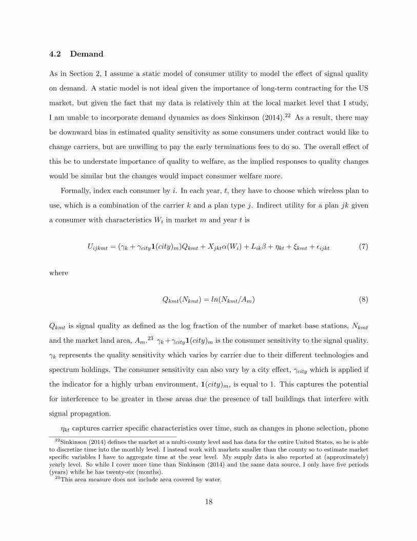
4.2 Demand
As in Section 2, I assume a static model of consumer utility to model the effect of signal quality
on demand. A static model is not ideal given the importance of long-term contracting for the US
market, but given the fact that my data is relatively thin at the local market level that I study,
I am unable to incorporate demand dynamics as does Sinkinson (2014).22 As a result, there may
be downward bias in estimated quality sensitivity as some consumers under contract would like to
change carriers, but are unwilling to pay the early terminations fees to do so. The overall effect of
this be to understate importance of quality to welfare, as the implied responses to quality changes
would be similar but the changes would impact consumer welfare more.
Formally, index each consumer by i. In each year, t, they have to choose which wireless plan to
use, which is a combination of the carrier k and a plan type j. Indirect utility for a plan jk given
a consumer with characteristics Wi in market m and year t is
Uijkmt = (γk + γcity1(city)m)Qkmt +Xjktα(Wi) + Likβ + ηkt + ξkmt + εijkt (7)
where
Qkmt(Nkmt) = ln(Nkmt/Am) (8)
Qkmt is signal quality as defined as the log fraction of the number of market base stations, Nkmt
and the market land area, Am.23 γk+γcity1(city)m is the consumer sensitivity to the signal quality.
γk represents the quality sensitivity which varies by carrier due to their different technologies and
spectrum holdings. The consumer sensitivity can also vary by a city effect, γcity which is applied if
the indicator for a highly urban environment, 1(city)m, is equal to 1. This captures the potential
for interference to be greater in these areas due the presence of tall buildings that interfere with
signal propagation.
ηkt captures carrier specific characteristics over time, such as changes in phone selection, phone
22Sinkinson (2014) defines the market at a multi-county level and has data for the entire United States, so he is ableto discretize time into the monthly level. I instead work with markets smaller than the county so to estimate marketspecific variables I have to aggregate time at the year level. My supply data is also reported at (approximately)yearly level. So while I cover more time than Sinkinson (2014) and the same data source, I only have five periods(years) while he has twenty-six (months).
23This area measure does not include area covered by water.
18

pricing, national coverage, national advertising, and spectrum that are not captured in the data.
ξkmt is the unobserved carrier characteristic that captures any idiosyncratic about demand for
the firm’s product. Xjkt are plan-type-carrier-year fixed effects, whose effects vary by consumer
characteristics Wi. I choose to use this instead of instead of explicitly using pricing and plan
characteristics since these vary little over time and not at all over markets. In particular, I eschew
estimating the intensive use of phone minutes in response to the fee structure since this is only
possible with minutes and specific plan data.24 Lik is great-circle distance between the consumer
location (in practice their population weighted zip code centroid) and nearest store that sells a
carrier’s plans, which matters as consumers may be more likely to buy a plan if they have to travel
a shorter distance to initially obtain or service the plan. β is thus the sensitivity to distance of
the nearest store. εijkt is an idiosyncratic i.i.d. random variable, which will rationalize consumer
adoptions of plans that are lower in deterministic indirect utility.
Define the mean (i.e. deterministic) part of utility as
δijkmt = Uijkmt − εijkmt (9)
I assume a type 1 extreme value distribution of the error. Thus the model is similar to the example
in Section 2, but there is added heterogeneity in terms of options (prepaid and postpaid) and in
consumer characteristics. This formulation yields the familiar logit formula for adoption probability
of plan jkt for consumer i:
Sijkmt(δimt) =exp(δijkmt)∑
k′inK
∑j′inJ exp(δij′k′mt)
(10)
With ex ante identical consumers, this would be almost exactly the same model as Section 2
where the only heterogeneity is in the random taste shocks. However, consumers are not identical
since I observe their characteristics and I allow this to affect their utility. Construed broadly,
taste shocks are now a combination of the logit error and the consumer-plan fixed effects. Thus
the observed heterogeneity allows the model to flexibly accommodate strategic complements and
substitutes at arbitrary mean utility levels and shares, since now the taste shocks in utility may be
multimodal.
24For an example of what can be done with such data, see Jiang (2013).
19

There is also an added effect that while the elasticities are functions of market shares within
groups of observably identical consumers, overall it is not as the overall elasticity is a mixture of the
group-level elasticities. As is well known, any discrete choice model with independent shocks has an
independence of irrelevant alternatives property (IIA) - the rate at which two goods are substituted
between each other by the same decision maker is independent of other options. Thus substitution
from an option, A, is most strong with the option with the highest probability and implied mean
utility, B. This is even though option A may be extremely similar (even identical) to option C.
In the context of the logit, this translates into the elasticity of substitution for an individual
being completely proportional to a function of the probability of that decision maker choosing
each option. For a given population of identical consumers, population elasticity becomes then a
function of market shares, but since I differentiate consumer utilities by observed characteristics,
the does not hold in my model.
Extensions of logit that weaken the IIA property by adding unobservable heterogeneity are
possible and widely used in the literature. These extensions would also weaken the two-toned
comparative statics from the toy model by adding even more taste heterogeneity. I report later two
alternative specifications - a nested logit taking the nests as the plan types, and a random coefficient
on quality. Nested logit can be thought of introducing a nest specific error term that when added
to the option-level error terms creates a nest-level logit error term.25 Random coefficients, on the
other hand, turns one or more of the coefficients on the explanatory variables into a random variable
itself. Nested logit is in some sense a variant of random coefficients - the random coefficient is on
a nest-specific fixed effect. The idea of both these approaches essentially is to add correlation into
the unobserved parts of the utility, so that the utility ex post shocks are closer for certain goods.
4.3 Supply
The industry game assumed for estimation is very similar to the example model in Section 2. Each
year t, the headquarters of firms k set national level prices simultaneously for all their products,
Pjkt. Their engineers then simultaneously set the number of base stations Nkmt at the market level
and the firm incurs marginal costs Fkmt of quality. In this industry, I find this timing more realistic
than the usual modeling assumption where quality is changed first since an individual engineer is
25See Cardell (1997) for a full treatment.
20

unlikely to consider the small price effect his local building decision has on the incentive to change
national price levels.
There are no adjustment costs in this model which could be considered unrealistic in this context
since there are raised costs when a base station is first installed. Given the limited amount of data
it is unfortunately not possible to estimate a fully dynamic model of oligopoly quality investment.26
In a growing market like wireless sunk costs are less important since the option value of waiting is
limited. Also, the carriers tend to treat their capital investments in annualized terms - they treat
the initial cost as part of that year’s borrowing, and the costs are spread over more than a decade
in repayments. Assuming that demand is static, actions year to year do not effect each other, so
each year can be thought as an isolated two stage game.27
The lack of dynamics has further benefit since I do not have data for the entire United States.
Without national level data I will not be able to simulate equilibria for the pricing aspect of the
game. But since the quality setting stage for one year has no effect on later periods, I can examine
each year’s quality stage alone taking prices as given.
Let Pjkt be plan specific prices, Ckt be constant carrier-specific costs, and Nmt be the vector of
all base station counts. Define also the demand Djkmt as the total sum of probability of adoption
of a carrier’s plan in a market-year over all consumers. Market profits are equal to markups times
demand, or
πkmt(Nmt) =∑j∈J
(Pjkt − Ckt)Djkmt(Nmt)− φk(Nkmt) (11)
As in 2, this is a normal-form game of complete information with a pure-strategy Nash Equilibrium.
The implied necessary condition of the equilibrium is
dπkmt(Nmt
dNkmt=∑j∈J
(Pjkmt − Ckt)∂Djk(Nmt)
∂Nkmt− ∂φkmt(Nkmt)
∂Nkmt= 0 (12)
As in the example model of Section 2, the cross partial of demand still determines the monotone
26Since demand is estimated at the year level, supply can only be estimated at the year level as well. In addition,while some of the data for supply reports dates for base stations to the day, these dates represent the day the basestation is reported or approved by the Connecticut state government. Other data is from collection from archiveswhich were collected randomly and do not have exact dates associated with. Given these level of imprecision, myaggregation to the year level seems to be prudent.
27Formally, I am making the assumptions that firms do not play history dependent strategies. Given my assump-tions, repeated plays of the static equilibrium is then an equilibrium for the infinite horizon game.
21

comparative statics of the model. These are explicitly derived in Appendix D, but in short, the
model without any heterogeneity in consumers would be almost exactly the same as the model
in Section 2 and would also have strategic substitutes for all the market structures observed in
the data. The consumer heterogeneity does allow for strategic complements though, but this is
dependent on having high enough amounts of consumer heterogeneity such that firms have a very
high market shares for particular segments of the population. Thus the comparative statics depend
on the heterogeneity parameters estimated in the demand system.28
5 Data
To estimate my model, I use a set of unique and detailed information on consumer and supply
choices in the state of Connecticut.
Demand is estimated from the 2008-2012 editions of the Nielsen Mobile Insights Survey, a
monthly survey that asks consumers about their wireless purchase decisions. Sinkinson (2014) uses
this dataset to examine the value of the exclusive iPhone contract to AT&T. The Nielsen dataset
reports carrier used, the plan type, zip code and consumer demographics. In reality, the number
of possible plans was estimated by consumer advice website Billshrink to be approximately 10
million.29 Given the data I have, I will simplify and say each carrier offers one of two composite
plans, prepaid or postpaid. I use income, household size, age and gender in the estimation as
they are likely to be especially important for taste variation in cell phone use. Income is likely to
affect price sensitivity; household size will proxy for the value of family plans that are very popular
options; age will proxy for the affinity for new technology; and sex might capture variation in calling
patterns across genders.
Table 3 shows the unweighted market shares for the 17,235 survey respondents. The data has
a shortcoming that only the four major carriers are identified, so all other carriers have to be
aggregated in an “Other” category. This is a problem in that prepaid brands Virgin and Boost
28Random coefficients or nested logit specifications could also introduce strategic complements since these segmentmarkets by consumers with unobserved variation in tastes for particular goods based on either their characteristiclevels or by nests. As I will present later, random coefficient and nested logit versions of the model do not have verydifferent results from the pure logit model with heterogeneous effects, implying that effects explain almost all of thevariation.
29billshrink.com closed down in 2013. An archived February 4, 2011 press release with this estimate can be foundat http://www.billshrink.com/blog/press-releases/americans-overpay-336-a-year-on-wireless/. More re-cently, a July 31, 2013 article in the Wall Street Journal, “Inside the Phone-Plan Pricing Puzzle” , notes there are750 smart phone plans from the four major carriers.
22

are not distinguished in the data. Both are owned by Sprint and use its network, so the supply
side will be somewhat misspecified in the sense that Sprint will not have all of its customers
included when calculating its profit. This discrepancy may not be so bad since a separate dataset
in my possession, from Scarborough Market Research, has approximately the same market share for
Sprint also including Virgin and Boost - 8.17% in Nielsen versus 9.42% in Scarborough.30 Verizon
is the market leader, followed closely by AT&T. Sprint and T-Mobile are distant also-rans, with less
combined market share than AT&T. The aggregation of all other plans, which vary from MetroPCS,
which owns its base stations, and Mobile Virtual Network Operators StraightTalk and Tracfone,
which license use of the network of other firms, is slightly more than 12%.
Postpaid plans dominate, with only 18% of respondents having prepaid plans. Penetration is
high, with only 11 percent without cell phones. In addition, a comparison of the raw data with
the American Community Survey five year estimates for 2006-2011 reveal that the two closely
correspond in demographics.31
The base station data was created from data published online by the Connecticut Siting Council,
the regulator of telecommunications sites in Connecticut. The national regulator of telecommuni-
cations sites, the Federal Communication Commission (FCC), does not collect comprehensive base
station information.32 In contrast, the CSC maintains two datasets meant to be as comprehensive
as possible and is therefore the best source of this kind of data in the US.
The first records information for all proceedings between the CSC and site applicants. The CSC
regulates siting on towers built explicitly to house base stations (as opposed to base stations on
preexisting buildings) and collocation (when there are multiple carriers at a single site, a common
occurrence given the high costs of developing a site). Thus for every tower and for every other site
with more than one carrier, I have information on when a base station was cleared for installa-
tion, geographic location, its owner and miscellaneous technical information like the site type and
sometime comments about the type of equipment installed.
The second dataset is taken from the towns which reports not only the information in the first
30The data is similar to the Nielsen dataset as it is also consumer-level observations, but it is not used for estimationdue to the fact that about half the observations about carrier choice have been imputed due to non-response usinga nearest neighbor algorithm. Imputation introduces unusual estimation issues, so the un-imputed Nielsen data isused instead.
31See Table 4.32The FCC has two databases. First, there is antenna data that is limited to only enough antennas to create
license boundary maps, and second, there is site data that is mandatory only for installations over 200 feet tall andinfrequently updated.
23

dataset but also sites on preexisting structures and only one carrier. This data is far less complete
than the CSC original data, and generally only has the location and base station owners. This
data uniquely reports about half the number of sites in the data, so I merge both datasets and use
only the ownership and location variables, which are consistently reported across both. Further,
the second dataset is continuously deleted and replaced with an update on monthly basis, sos older
copies had to be retrieved using the Internet Archive.33 Archiving of sites is not done with perfect
regularity, so the dates of the site copies available vary from year to year. Due to the fact that
sites are often not operational when first recorded by the state regulator, I define the count of base
stations for a year as the count of all base stations reported before January 1st of that year.
I define the market as the PUMA, the smallest level of geography in the Public Use Microdata
Sample (PUMS). Each of the 25 Connecticut PUMAs has at least 100,000 people in it so that the
identities of sample respondents are protected. According U.S. Census documentation the PUMAs
are designed to represent existing communities whenever possible with similar characteristics.34
I therefore use the PUMAs to approximate travel patterns. The 2010-2011 Regional Household
Survey records detailed information about travel behaviors in the New York commuting area,
which includes Fairfield and New Haven counties in Connecticut. While not comprehensive enough
to use for in estimation, the data show that 53.6% of trips taken by Connecticut respondents are
intra-PUMA. Out of these market I designate PUMAs 8, 19, 20 and 24 as the “city” markets which
have added effect on the quality sensitivity coefficient. Respectively, these PUMAs are downtown
Waterbury, Hartford, New Haven and Bridgeport, which are the densest PUMAs by population.
PUMA 23, downtown Stamford, would normally qualify as well, but due to the fact that PUMA
23 bisects PUMA 25, I merged 23 and 25 to maintain contiguity in markets, so in practice that
market as a whole combines urban and suburban areas.
Examination of Table 5 shows that AT&T has on average the most base stations per PUMA,
and Verizon has the least. Verizon is the market leader in the data and in the nation as a whole,
and has a reputation for high signal quality. Thus much of the overall quality in Verizon’s case must
be either explained by aspects other than base station placement or by higher average productivity
per base station. During estimation, I control for this via the carrier-specific quality sensitivities
33The Internet Archive (www.archive.org) is website that archives other websites. By using the site’s “WaybackMachine” function, one can access old versions of websites that they have stored offline.
34See “A Compass for Understanding and Using American Community Survey Data”, February 2009.
24

per base stations and by the carrier-year fixed effects.
Store location information was taken from ReferenceUSA. In Autumn 2013, I recorded the loca-
tions of all stores in Connecticut that contained “cellular” or “mobile telephone” in their Standard
Industrial Classification (SIC) title. I further hand cleaned this list and determined carrier selection
via web searches when possible. Clearly, this measure is imperfect since I am including only store
locations from after my sample period - there will be stores I include that will not have opened yet
and some stores that were active had closed. However, the inclusion of the variable is potentially
important as it explains geographic variation in carrier selection that might otherwise be attributed
to base station placement.
6 Estimation and Results
6.1 Endogeneity of Quality
Typically economists worry about the endogeneity of price in demand estimation due to unobserved
demand shocks. In the application of wireless telephony that is less of a concern because pricing
is done at the national level. As noted earlier, I eschew estimating price elasticity directly and
absorb all the corresponding variation in fixed effects. Instead, there is a need to correct for the
endogeneity of quality to the unobserved component of demand. Formally:
E[Qkmtξkmt] 6= 0 (13)
That is, since base station placement is endogenous the carriers may have placed base stations ac-
cording to some unobserved components of demand. For example, some areas might have especially
high interference due to unique geography or buildings configurations. Thus a carrier might place
more base stations to yield to same signal quality, thus biasing the estimates of quality sensitivity
downwards. Alternatively, a firm might decide to advertise new base station deployment in a mar-
ket - which would boost demand but be confounded with the increase in base stations, biasing the
quality sensitivity upwards.
Traditional methods for dealing with endogeneity in demand systems employ instruments that
are actually infeasible in this setting. Berry, Levinsohn, and Pakes (1995) use product charac-
teristics of rival products to instrument for price, under the rationale that attractiveness of rival
25
products would shift demand for the good in question. In that context product characteristics
were assumed exogenous due to the long product development cycles in automobiles. Alterna-
tively, Hausman, Leonard, and Zona (1994)and Hausman (1996) use prices in other regional cities
as instruments for price, citing some unobserved regional component of a firm’s costs common to
all markets. Neither of these can be implemented here since the product assortment and pricing
for all markets across all times is the same. Quality does vary by market, but the carrier-year fixed
effects use all the variation that could be attributed to the Hausman-style instruments.
Instead, I use a cost side instrument that would influence a firm’s incentives to build base
stations, the fraction of a town’s zoning regulations that are telecommunications related. Industry
sources note the primary difficulty with siting is the cost and delay in proceedings with local zoning
authorities, which is greatly hampered by long and ambiguously-worded statutes. If a town devotes
more space to telecommunications facilities then they must be more worried about it relative to
other kinds of zoning.35 Using the ratio of the number of characters used rather than just the
characters in the telecom sections since this corrects for the fact that some towns might simply
have longer, wordier regulations. Since there are multiple towns in a PUMA, I use the population-
weighted average. With the firm and city interactions, I need four additional instruments. I
therefore also use the interaction of regulation with firm and city.
Regulation has a major drawback as an instrument in that it does not vary by firm, but only
by market. Regulations further do not vary by year since I collected them over the period of 2012-
2013, and thus the regulations reflect current law in those states. However, there does not seem
to have been radical changes in the telecom sections of the zoning codes as many zoning codes
include references to amendments and their dates. Also the use of a weighted average mitigates
any potential unobserved change by a particular city. Thus the instrumenting strategy precludes
inclusion of a market level fixed effect and will not exploit firm level or time variation.
35Admittedly, Connecticut is unique since final authority lies with the state for development of new structures fortelecommunications and additions of new base stations on preexisting sites. Towns only have de facto control over thefirst base station on a preexisting structure. When making its decisions, the Connecticut Siting Council can actuallyignore all town zoning laws if it so chooses. However, towns must still be consulted by carriers, and a good faith effortmust be shown to adhere to the town regulations as closely as possible. Also, towns may object to applications madeto the council. As a result, carriers sometimes negotiate Connecticut towns for years. Thus the regulation variable isnot so much a measure of de facto regulation strength but of potential pushback from the local community for anyproposed base station and difficulty negotiating with them.
26
6.2 Demand Estimation Procedure
Even with instruments, dealing with the endogeneity is not straightforward. ξkmt cannot be esti-
mated as a fixed effect because it is not separately identified from quality. The typical procedures
for endogeneity in demand estimation, introduced in Berry, Levinsohn, and Pakes (1995), requires
aggregate market shares, and the data is not large enough for me to confidently use the shares
found therein.36 In this case, I have 17,235 survey responses, which collapsed to the 480 carrier-
market-years would have too much noise to be used in this way. For example, some markets are
as small as 29 individuals in a year. I instead adapt a suggestion made as an aside in Berry (1994)
and most prominently applied in Goolsbee and Petrin (2004), in which fixed effects soak up all
the variation at the carrier-market-year level in a first step, and then covariates of interests are
regressed on these fixed effects in a second step.37 The second step allows for linear instrumental
variables regression since the endogenous error terms enters linearly into the fixed effects.38
Define the variable that absorbs all carrier-market-variation as
ζkmt = (γk + γcity1(city)m)Qkmt + ηkt + ξkmt (14)
so
δijkmt = ζkmt + Liktβ +Xjkmtα(Wi) (15)
I then conduct maximum likelihood over the observed individual choice probabilities by solving
the following objective function:
arg maxθ={ζkmt,γk,γcity ,β,α}
∑i∈I
ln(Sijkmt(θ|Qkmt, Am, Likt, Xkmt,Wi)) (16)
In practice Xjkmtα(Wi) is simply different for every plan-type, carrier, year and characteristic
36The sample size by market-year varies from 29 for New Haven in 2010 to 331 in 2008 for the Windsor Locks area.37Technically, Goolsbee and Petrin (2004) do use use the procedure in Berry, Levinsohn, and Pakes (1995), which
takes the observed markets shares as given to imply unique values for the fixed effects. Like me, however, they breaktheir estimation into two parts, and do not simultaneously estimate the parameters of the endogenous variables, asin Berry, Levinsohn, and Pakes (1995). They also note that they could have estimated the fixed effects rather thanuse the procedure in Berry, Levinsohn, and Pakes (1995), but simply chose not to, presumably for computationalconcerns.
38An alternative would be to use a control function, as in Petrin and Train (2010), though I decline to do so dueto the strong assumption of the independence of the instruments with ξkmt, rather than just no correlation.
27

combination so I estimate a corresponding fixed effect. Once ζkmt is recovered I can then estimate
γm via instrumental variables using (14) as the estimating equation and Zkmt as instruments. While
there is error in the measurement of ζ, the linear form allows that error to be absorbed into ξkmt. I
weight using the standard errors for ζkmt from the maximum likelihood step for efficiency reasons.39
Identification in this model depends on variation in choices over the different markets and time.
Identification of the quality sensitivity terms are identified across markets within a carrier-year,
as we employ carrier year effects. The distance terms are identified from variation across markets
and within markets as these are zip code specific. The product-demographic specific terms are
identified from the relative share of products in the sample for that demographic across markets,
and brand-year-market effects are identified from the shares for that brand in that market year.
For comparison, I also present results from the nested logit specification and a random coefficient
specification. The nested logit uses the plan types - none, prepaid and postpaid - as nests and
estimates a single dissimilarity parameter, λ, which approaches 1 as the model approaches pure
logit. Plan type was used for the fact that prepaid customers might be different from postpaid
customers on some unobservables since they prefer a plan that they can make cheaper on average
through lower utilization and postpaid plan requires a good credit record. This means that different
carriers are not directly dissimilar since every carrier (except Sprint) has a product in prepaid and
postpaid, but since T-Mobile has much more successful prepaid product than AT&T or Verizon,
the overall substitution between the firms should differ.
For the random coefficients specification, I assume no nesting and that the quality sensitivity
coefficient is distributed normally. With a normal quality sensitivity, the mean of the coefficient is
additively separable and is absorbed into ζkmt. Thus the quality sensitivity can still be instrumented
for in the second step and while the standard distribution of the distribution can be recovered from
the first step by integrating over an interaction between the quality and a random variable with the
standard normal distribution. Rather than simulate, I use numerical Gauss-Legendre quadrature
on 15 points, which is both computationally simpler and more accurate than simulation. The high
accuracy of quadrature obviates the need for correction of the standard errors due to simulation
error.
39I could do the maximum likelihood and the linear steps in a single-step GMM procedure in which the momentsare the score of the maximum likelihood and the exogeneity conditions of the linear step. This would be similar toBerry, Levinsohn, and Pakes (2004), although in that paper they also exploit data on second-best choices.
28
6.3 Results: Individual Identified Demand Parameters
In the MLE step, I estimate ζkmt along with all parameters that capture variation at the consumer
level. This includes the plan-consumer-characteristics-year effects and the β store distance sensi-
tivity term. For the nested and random coefficient terms, λ and σ are also presented, respectively.
The results from all three specifications are nearly identical, with a McFadden’s Pseudo-R2
of 0.25. There is in fact only a difference of less than 0.2 log points between any of the three
models, and clearly a likelihood ratio test fails to distinguish between them. For the nested logit
specification, λ is 1.09, which is generally not consistent with utility maximization.40 However, the
value is not significantly different from 1, reflecting the already established fact that the nested logit
model does not explain any further variation than the pure logit model. The random coefficient
estimated is also relatively small at 0.08 and not significant. A formal test of the multinomial logit
from Hausman and McFadden (1984), in which the model is reestimated on data without one of the
options to see if the estimate parameters are the same, are presented in Table 7. The test statistics
suggest no evidence that the true model is not multinomial logit.41
One can think of the nesting and random coefficients as adding more ex post heterogeneity to
the logit - observationally identical populations of consumers have different distributions of ex post
utilities for options which will cause their substitution to differ from the markets shares of the total
population. Given consumer characteristics, product and year specific fixed effects, there is not
much much variance that this unobserved heterogeneity can explain. Moreover, there are not many
options (10 in total), which further lessens the available variation. Given the lack of difference
between the models, and that there is substantial heterogeneity in utility given by the fixed effects
would break the IIA property at the market level, I continue with the pure logit with individual
level heterogeneity as my preferred specification.
In all specifications β is negative as one would expect, though it is very small in all specifications,
and not significant. The implied own-elasticity of travel distance to stores is essentially zero, so I
ignore this aspect of demand in the subsequent analysis.
40I say “generally” since Borsch-Supan (1990) shows that dissimilarity parameters greater than 1 may be possiblein a utility maximization framework given certain values of the covariates.
41Three out of five of the tests are actually negative, which is odd given this is a Chi-square test. However, inpractice this test is often negative, as in the original application of Hausman and McFadden (1984). They tooknegative values to be a sign of no evidence of a difference between the multinomial logit and the true model, and Ifollow that in line with the subsequent literature.
29

The estimates of the plan-type, carrier, year and characteristics effects are too numerous to
report completely, so I will report them in part. The year specific product effects for the prepaid
products are in Table 8. These represent the difference in utility from prepaid products relative to
postpaid products for every year and carrier. These results imply that value of prepaid products
generally grew over the sample period for all carriers. The results also show that prepaid is an
inferior product relative postpaid - except for Other which has large positive estimates revealing
that its prepaid plans are actually significantly better.
The remaining coefficients are the difference in plan utility compared to a 35 to 65 year old
woman in a multi-person household that earns between $50 to $75 thousand a year. Instead of
reporting all 444 remaining estimates and standard errors, I report in Table 9 the mean and in
parenthesis how often the estimate was estimated to be different from 0 with 95% significance.
About 37% of these estimates are significant at the 95% level. Prepaid value effects are estimated
with less accuracy in general given the lower number of prepaid purchases. In general, the estimated
effects are quite small and do not vary strongly across firms. The same trends are true for most of
the firms - the poor, the old and those living alone have less values for phone service. In particular,
old seem to prefer postpaid plans in the ”Other” category more than other demographics. Also,
the value of prepaid plans of the Other composite brand is actually greater for poor individuals.
6.4 Results: Quality Sensitivity Parameters and Brand-Year Effects
Given the MLE results for the preferred specification, linear instrumental variable estimation can
proceed with the carrier-market-year fixed effects. Table 10 examines the strength of the regulation
instrument. Weighted regression of the instrument on Qkmt is very significant, and remains so on
subsamples divided by the different carriers and for the city markets only. The weights used are the
same for instrumental variables regression itself, the estimated variance of the carrier-market-year
fixed effects. Using the multiple-endogenous F-Statistic suggested in Angrist and Pischke (2009,
p. 217-218) yields very large values that are greatly above the rule-of-thumb value of 10 suggested
by Stock, Wright, and Yogo (2002).
Estimates from both an instrumented regression and an un-instrumented regression demonstrate
significant differences between the firms in quality sensitivity. Relative to AT&T, T-Mobile and
Sprint having significantly higher quality sensitivity and Verizon a negative one. The city effect
30

on quality sensitivity, as expected, is significantly negative. Instrumenting matters: the baseline
sensitivity γAT&T of 0.15 doubles to 0.30, while the other effects all become more positive. The
downward bias correction is especially important for the Verizon parameter, since weighted OLS
implies it is slightly negative. Though not significant, this would imply improvements in Verizon
signal quality reduce market share. In the case of cities, the total coefficient would be even more
negative. After instrumenting, this is no longer the case: net effect of Verizon quality becomes 0.16
outside cities and 0.02 within. Nevertheless, Verizon ends up being problematic - the sensitivity
in either case not significantly different from zero nor is it significantly different from AT&T. In
contrast, marginal effects from signal quality can be differentiated between AT&T, Sprint and
T-Mobile both with and without instrumenting.
The results have a curious implication - the firms with higher market share, AT&T and Verizon,
have less marginally productive base stations than the smaller carriers, T-Mobile and Sprint. This
compounds the earlier puzzle that Verizon has the least base stations on average even though it is
the leader by share in most markets in the sample. This apparent contradiction can be resolved by
recognizing that a more convex production function of signal quality in base station density will
have a smaller γk but a higher intercept ηkt. As noted earlier Verizon and AT&T have more and
better spectrum than their rivals, and as early entrants may have access to better site locations
compared to Sprint and T-Mobile. Thus they may have reached the flat part of their production
functions much earlier than Sprint and T-Mobile, resulting in the observed relationship between
base stations density and market level quality to be very flat relative to their rivals.
To illustrate this idea, Figure 2 plots the implied mean quality on base station density for the
year 2012. The curves are equal to
(γk + γcity1(city)m)ln(Nkm2012/Am) + ηk2012 (17)
As you can see, while the plots are quite flat for AT&T and Verizon for most of this range, the
average level is much higher than Sprint or T-Mobile. Thus an average AT&T and Verizon base
station is estimated more productive than T-Mobile or Sprint base station, it is just that this benefit
is very front-loaded in the former case.42
42A difficulty with this interpretation is that the carrier effect also contains all other carrier specific differences, soestimated intercept of this function is not separately identified from things like phone selection, pricing, spectrumholdings or even branding. So while I can interpret some of the difference in fixed effects as differences in the
31
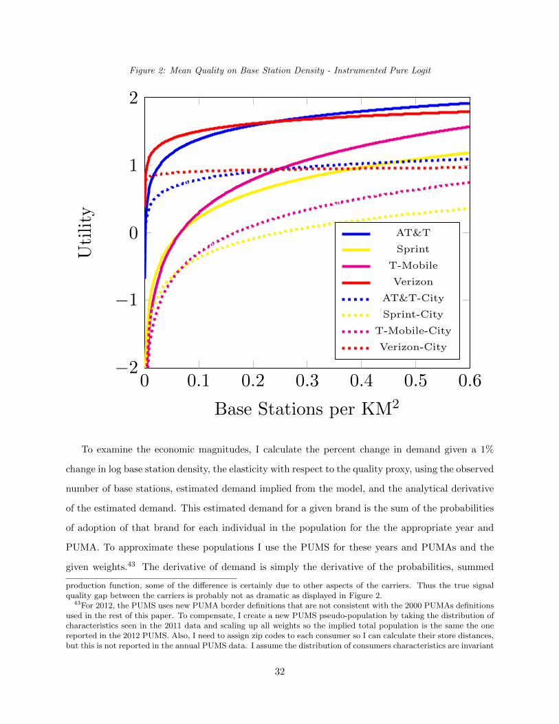
Figure 2: Mean Quality on Base Station Density - Instrumented Pure Logit
0 0.1 0.2 0.3 0.4 0.5 0.6−2
−1
0
1
2
Base Stations per KM2
Uti
lity
AT&T
Sprint
T-Mobile
Verizon
AT&T-City
Sprint-City
T-Mobile-City
Verizon-City
To examine the economic magnitudes, I calculate the percent change in demand given a 1%
change in log base station density, the elasticity with respect to the quality proxy, using the observed
number of base stations, estimated demand implied from the model, and the analytical derivative
of the estimated demand. This estimated demand for a given brand is the sum of the probabilities
of adoption of that brand for each individual in the population for the the appropriate year and
PUMA. To approximate these populations I use the PUMS for these years and PUMAs and the
given weights.43 The derivative of demand is simply the derivative of the probabilities, summed
production function, some of the difference is certainly due to other aspects of the carriers. Thus the true signalquality gap between the carriers is probably not as dramatic as displayed in Figure 2.
43For 2012, the PUMS uses new PUMA border definitions that are not consistent with the 2000 PUMAs definitionsused in the rest of this paper. To compensate, I create a new PUMS pseudo-population by taking the distribution ofcharacteristics seen in the 2011 data and scaling up all weights so the implied total population is the same the onereported in the 2012 PUMS. Also, I need to assign zip codes to each consumer so I can calculate their store distances,but this is not reported in the annual PUMS data. I assume the distribution of consumers characteristics are invariant
32

over all the individuals.
I report medians of demand elasticities of base station density across markets and years in Table
13,in terms of what a 1% change in log base station density, the signal quality proxy, would do to
market share.44 A 1% change Verizon’s signal quality has the smallest own-effect, giving Verizon
0.13% more of the market for the median market-year. AT&T has the highest effect (0.25%) while
the effect is intermediate for Sprint (0.16%) and T-Mobile (0.18%). The fact that AT&T is the
highest despite it’s relatively low quality sensitivity parameter suggests the importance of its other
quality dimensions, such as spectrum and the exclusivity of the iPhone.
As a result of the relative unimportance of the consumer characteristics-based heterogeneity,
people agree largely about how the carriers are ranked. Thus, people who selected options providing
less mean utility, like Sprint and T-Mobile plans, must have gotten a large idiosyncratic taste shock
for that option. As a result, substitution away from those firms is low when rivals increase quality
- these vary between -0.1% to -0.3% for the median market year.
In contrast, consumers of AT&T and Verizon are not particularly loyal since most consumer
chose them because of their high mean utility - if something better in mean utility comes along
they are more likely to switch. Thus substitution from AT&T is on average -0.06% of the market
and from Verizon between -0.13% to -0.06%. In terms of diversion ratios, AT&T and Verizon are
very substitutable with their rivals so have the most share poached from quality gains: AT&T
and Verizon steal half of their gain from each other when they improve quality, while Sprint and
T-Mobile steal about a third from either AT&T and T-Mobile. Notably, Sprint and T-Mobile are
not very good substitutes - they steal only about 10% of their gain from each other. In any case,
the cross effects of quality are relatively small, with no effect in any market year exceeding -0.27%
market share per base station.45
Finally, the estimates imply that base stations are strategic substitutes, since there seems to
be no dimension in which a firm dominates the market, i.e. even conditional on consumer char-
acteristics, market share is never greater than 0.5. As mentioned earlier, characteristics do not
seem to add a great deal of heterogeneity into tastes, so carriers do not split up the market into
within a PUMA, and then assign the PUMA population according to the proportions in the 2010 Decennial Censusdata.
44The median 1% change in the proxy is equivalent about a 1.2 base stations change over all the market years.45Interestingly, a combination of changes in preferences for products and increased quality overall results in elas-
ticities going down for Sprint and T-Mobile over the sample period. See Table 13.
33
segments which they individually dominate.46 While there is variation in market specific factors
like base stations across firms, firms only have more than 50% market share three times in the
Nielsen sample. Using the estimates the predict market share for the our pseudo-population of
PUMS respondents, 99% of the implied probabilities of adoption for each option by each individual
are below 0.5. Thus aggregate cross partial of demand with respect to signal quality is negative,
implying strategic substitutes.
6.5 Supply Side Estimation and Results
I back out a cost for each firm in each market-year for each carrier using the first order condition:
∑j
(Pjkt − Ckt)∂Dkmt(Nmt)
∂Nkmt=∂φkmt(Nkmt)
∂Nkmt(18)
Calculation of the left hand side of this equation (the marginal variable profit) requires prices and
marginal quantity costs to be known or estimated. Selecting a price to use for Pjkt is problematic
in my application since I aggregate over many products and products have a usage aspect which
means each individual could potential pay a different effective price. Instead of arbitrarily selecting
a price for a particular focal plan, as Sinkinson (2014) does when he uses the introductory smart
phone plan fee, I use the average revenue per user or (ARPU) reported in the UBS’s analysis of
the US wireless industry. ARPU is the main revenue measure used by industry participants. It is
also the variable used by the BLS to construct their price index for cellular phone service. Given
that I need Pjkt purely as an marginal revenue number, ARPU seems like a sensible proxy.
Marginal consumer costs Cjkt would usually be estimated via a price first-order condition, but
I do not have the nationwide data to estimate a first order condition on price. In principle, I could
estimate it as a free parameter for the first order condition of base stations, but in practice the term
Pjkt∂Dkmt(Nmt)
∂Qkmtis nearly collinear with ∂Dkmt(Nmt)
∂Nkmt. I instead take the “Costs of Wireless Service”
reported by the UBS analysis, and divide by the total number of consumers. This implicitly assumes
cost is constant across markets, which seems reasonable given carrier do not offer specialized plans
or phones by market.
The median base station cost per month is $8,147, which is about twice as much the numbers
46One can note Table 14, which shows correlation across products in the value of mean utility in the sampleattributable to consumer demographics and year only.
34

assumed by the engineering paper by Claussen, Ho, and Samuel (2008) or Bjorkegren (2013).
Those estimates were based on pecuniary costs alone, and did not include costs that come from
regulatory costs from negotiating with towns or meeting particular zoning codes. This implies that
non-pecuniary costs, i.e. delays caused by regulatory proceedings or negotiations, are significant
drivers of economic cost.
Costs do appear different by firm, with median across all markets and year being $11,605,
$8,230, $7,354 and $6,970, for AT&T, Sprint, T-Mobile and Verizon, respectively. Variance overall
is quite high, with a standard error of $5,263 across all market-years and carriers. Given the very
high variance, I elect to use the entire term Fkmt as the cost, rather a mean over year or markets.
Doing so allows me to retain heterogeneity in the used firm costs.
The size and variation in base station costs lead them to be an important strategic consideration,
and shows how important inframarginal signal quality is. For example, in 2012, the estimates imply
that T-Mobile spent 62% of its variable profit in Connecticut on base stations. Ratios are smaller
but still large at other carriers: with 46% (Sprint), 19% (AT&T) and 9% (Verizon).47 Thus signal
quality is both 1) important enough to firms to commit significant resources to, and 2) where gains
in efficiencies could be very beneficial to the firm.48
To investigate how my regulation instruments compares with cost I decompose the marginal
quality cost in two ways:
∂φkmt(Nkmt)
∂Nkmt= Hkmtψ + νkmt (19)
and
∂φkmt(Nkmt)
∂NkmtAm = Hkmtψ + νkmt (20)
The former is self-explanatory: the marginal quality cost is a linear function of regressors Hkmt
plus an error term. The second specification posits that costs are constant in density, and not base
stations, which may be plausible given that as firms continue to build in the same area, the costs
of finding new suitable locations would increase. Hkmt includes all possible costs shifters for firms,
47The variation in ratios is largely due to the difference in elasticities with respect to base stations and owndemand - with a higher elasticity the greater the relative gain from investment will be. Accordingly, these proportionscorrespond closely to those elasticities, which are not reported but available upon request.
48See Table 16 for ratios over multiple years.
35

but for my purposes I include a constant, fixed effects for firms besides AT&T, interactions of these
terms with the regulation instrument, and a fixed effect for the city markets. I then regress Hkmt
on the LHS of the above equations.
The constant in base station model returns estimates that imply the regulation variable decreases
the cost of base stations for all firms, which contradicts the rationale for using the instrument.
However, the second model implies that cost per base station density does increase with regulation.
Given that the model also seems to fit better with an R2 of 0.64 compared to 0.25, I prefer the
density model as the explanation of how the regulation variable contributes to costs. Looking at
the other results for that model, the intercept of density costs of AT&T is much lower than that
of its rivals, while AT&T is effected much more by regulation. This may be because of differences
in the skill of a carrier’s regulatory staff or because a larger firm like AT&T or Verizon has more
resources to devote to regulatory issues.
Presumably, there are many omitted variables in this regression, as site leasing fees, construc-
tion, backend, and power fees that should all contribute to the cost of installing and running the
base stations. As a result, I am not confident that the model estimates of ψ are robust enough to use
in counterfactuals, which is another reason why I prefer to use the entire terms ∂φkmt(Nkmt)∂Nkmt
which
includes the large amount of variation from market specific variation that the current regression
cannot explain.
7 Counterfactuals: Mergers of a Small Carrier
To learn about the impact of market consolidation in this industry, I examine two merger proposals
that recently have been pursued: the attempted acquisitions of T-Mobile by AT&T in 2011 and
then Sprint in 2014. The AT&T attempt got quite far in the approval process until it was ultimately
abandoned in December of 2011 after the Department of Justice decided to oppose it. The Sprint
attempt only got as far as discussions when it was abandoned in August. Allegedly, this was due
to concerns that the merger would also be ultimately opposed as well, demonstrating government
concerns about mergers in this industry overall.49 While these proposed mergers actually failed
and thus are unlikely to be attempted again, they should resemble the most likely mergers to be
49See “Sprint Abandons Pursuit of T-Mobile, Replaces CEO,” Wall Street Journal, August 5, 2014,http://online.wsj.com/articles/sprint-abandoning-pursuit-of-t-mobile-1407279448.
36

proposed in the future - acquisitions of small regional carriers like Alltel or Pocket, which in their
regions might have comparable market share to T-Mobile.
Counterfactuals are conducted using the state of Connecticut, as the costs so far estimated are
specific to the markets I have supply data for. As with the cost estimation, I used the PUMS
sample with the Census-assigned weights to simulate population level demand. To correspond
closest with current conditions and long-run outcomes, I set the counterfactuals in 2012 and use
the corresponding parameters and PUMS data.50 Inferences will be limited to Connecticut, but
this should give a good idea of what would happen nationally given that the market shares are
not widely different from reported national levels, and individual level characteristics (which are
different from the national average) are not overwhelmingly important in determining demand.51
I find equilibrium levels of quality by use of a fixed point algorithm, a la Morrow and Skerlos
(2011). One can rewrite the first order condition ( 18) explicitly using the chain rule:
∑j
(Pjkt − Ckt)∂Dkmt(Qmt)
∂Qkmt
dQkmtdNkmt
=∂φkmt(Nkmt)
∂Nkmt(21)
Conveniently, base station count appears as the denominator of the derivative of signal quality due
to the log specification, so I can write:
(γk + γcity1(city))∑j
(Pjkt − Ckt)∂Dkmt(Qmt)
∂Qkmt
(∂φkmt(Nkmt)
∂Nkmt
)−1
= Nkmt (22)
So I only need to calculate the right hand side of the equation given a guess for Nk′mt for all firms,
which produces a new guess, which produces a new right hand side, and so on until convergence.
Uniqueness is an issue, since it is not guaranteed in this setup with strategic substitutes. I have
tried various starting values for the counterfactuals and have found no other equilibrium, but it
may be possible that other equilibria exist. The players are very asymmetric, so there may be less
of an issue with multiplicity than if they were very similar.52
Pricing is certainly important to judging counterfactual situations in mergers, and was the main
focus of the AT&T-T-Mobile merger review. I have abstracted from pricing for the most part in this
50As noted earlier, I use the 2011 PUMS data scaled up to the 2012 Connecticut population for 2012 since geo-graphical definitions of the PUMAs changed.
51In particular, one should also note that Connecticut is the 4th densest state and the most wealthy.52In particular, with identical players one have problem with asymmetric equilibria in which players play different
strategies but there is no guidance on which player will play which strategy.
37

paper since national pricing makes identification of price sensitivity difficult and I cannot match
the national-level first order condition to my state level data. Up to this point, all the estimates
are valid given the assumption that pricing is done in a first stage before the base station decisions,
but a merger between the firms looked at in the counterfactuals would be at the national level and
so pricing incentives would change.
Given I cannot exactly model the equilibrium price adjustment, I instead simply note that the
counterfactuals would all likely lead to higher equilibrium prices as I do not assume any marginal
consumer cost efficiencies. Either there are less products, or cannibalization effects of lower prices
are internalized, so the incentive to price higher increases. I therefore run each counterfactual with
both no price adjustment and a 5% price adjustment for all firms. I chose 5% since it seemed that
if merger authorities expected a price increase any higher they would have blocked the merger,
irregardless of any quality adjustments.
One further wrinkle is that the effect of a merger is mediated by the price impact on utility. I did
not estimate this, so I appeal to the literature for guidance, using previously estimated own-price
elasticity for wireless phone plans to calibrate the counterfactuals. Unfortunately, there is significant
variance in the elasticities estimated - for example, Sinkinson (2014) reports own elasticities of price
of -1.4 from Verizon and -1.5 for AT&T.53 In contrast, Jiang (2013) reports much higher elasticities
for the fixed fees of contracts: -5.33, -6.92, -5.09 and -4.78 for AT&T, Sprint, T-Mobile and Verizon,
respectively. Jiang (2013) also reports an industry own-price elasticity (with respect to having no
phone at all) of -0.61, which is much higher than Miravete and Roller (2004)’s report of -0.13, the
lowest estimate that I know of in this literature.
Casual empiricism implies that the Sinkinson (2014) is more believable for my sample. Un-
der Nash-Betrand pricing (and assuming no other endogenous variables), the equilibrium percent
markup is equal to the negative inverse of the own elasticity, the so-called Lerner Index.54 For post-
paid plans, the implied elasticities under this rule are between -1.11 and -1.36 in our sample, and
for prepaid plans between -1.15 and -2.47. The Jiang (2013) elasticities are clearly much higher and
53As he is using the same dataset, Sinkinson (2014) also has no market variation in price, and very little variationacross time since his panel is short. He instead relies on product characteristic variation in both service and phonesand does not use product level effects as I do. Price then is used to explain product-year level variation in shares,while controlling for as much of the demand variation as possible. In particular, he has Nielsen data from drive teststhat actually measure dropped call rates, providing variation on roughly the MSA level, which is much larger thanthe market I examine.
54See Lerner (1934).
38

might suggest that elasticities have changed significantly over time. Jiang (2013) looks at a sample
period from 2000 to 2001, while Sinkinson (2014) is much more recent, looking at 2008 to 2010. I
therefore find the price coefficients to match Sinkinson (2014)’s price elasticity for AT&T and then
Verizon in my data for the years 2008 to 2010, and then take their average as the coefficient I use
in estimation.
I also run counterfactuals holding the actions of non-merging firms fixed. I call this the “Uni-
lateral” case, and I do this to examine how much the actions of non-merging firms have on the
equilibrium. When I allow firms to adjust prices in the unilateral case I only allow the non-merging
firms to do so.
I use the three scenarios from Section 2 again, and since base stations are strategic substitutes,
then comparative statics from the logit example still hold. I explain the theoretical forces at work
in detail in Appendix B. I review the results of each below, organized by the scenarios.
7.1 Discontinue All Products from Purchased Firm (*)
Here the counterfactual is the same whether AT&T or Sprint buy out T-Mobile - T-Mobile products
leave. The only difference is how much the lump sum transfer is and who is paying it, but that
is outside of the scope of the model. Given our finding of base stations as strategic substitutes,
I find that when T-Mobile leaves, the remaining firms increase their base station density. For
example, holding prices fixed AT&T would increase base stations by 2.90%, Sprint 8.15% and
Verizon 2.46%. In the unilateral cases actions for the firms allowed to move resemble quite closely
the full equilibrium case. For example, holding prices fixed and allowing only the acquirer to move,
AT&T would increase base stations by 3.14% and Sprint 8.75%.
However, even when holding prices fixed there is a net consumer welfare decrease of $1.35
per consumer. Given no price change, this must come from the loss of T-Mobile variety and the
substitution of some consumers to the Other composite carrier and the outside option. This only
gets worse as prices increase 5%, as per capita monthly consumer welfare losses increase to $3.42.
When all prices are allowed to adjust, quality increases are actually higher, as the price increases
marginal revenue from each new consumer. However, the price increase of 5% seems to be too
high for Sprint moving alone, since the profit is not as high when price is held fixed and quality
actually reduces slightly. The AT&T merger with a 5% price increase also has lower profit for
39

AT&T without accommodation, which suggests that the unilateral price increase for this merger is
actually less than 5%.
Profit of the acquirer is larger than sum of their pre-merger profit and T-Mobile’s in only some
of these counterfactuals. These mergers can be rationalized with variable profits alone without
outside fixed savings. This happens in the equilibrium case with AT&T, and in the unilateral case
with AT&T with no price changes. In contrast, none of the Sprint mergers can be justified, due
to the fact Sprint is not large enough so that the benefit to Sprint’s profit can make up for the
complete loss of T-Mobile’s. Thus a merger with small brands would likely prefer to retain both
brands in some form.
7.2 Retain Products from Purchased Firm with Separate Networks (**)
When the acquirer does retain T-Mobile and the two networks do not integrate at all, the outcome
depends greatly on whether AT&T or T-Mobile is the acquirer. When the acquirer is large, i.e.
AT&T, almost all the T-Mobile base stations are removed, since the AT&T products have a much
higher mean utility, net of their network. The counterfactual then ends up resembling the dropped
products case very closely, since T-Mobile is practically dropped. Without price changes, base sta-
tions for AT&T actually rise on average since the drop in signal quality of T-Mobile is so great that
the strategic substitutability of base stations overcomes the internalization of the cannibalization
effect.
When the two merging parties are more similar, as when Sprint is the acquirer, the adjustment
in base stations is not so asymmetric. T-Mobile does lose a significant amount of base stations
absent price changes, but Sprint also decreases a few percent on average. The equilibrium case
is therefore better for consumers than when AT&T was the acquirer, so that consumers, holding
prices fixed, only lose $0.23 a month rather than $0.98, and, increasing price by 5%, they lose only
$2.30 a month rather than $3.00.
Mergers are more profitable in this scenario than in ∗, since firms can profit off consumers who
have such high taste shocks for T-Mobile they still buy it even when the quality degrade significantly.
Again, the only case where the profit does not justify the merger for AT&T is the unilateral case
where price increases. The Sprint mergers are also profitable for all but the unilateral case with
price change, in contrast to ∗ where Sprint cannot benefit from the T-Mobile product line.
40
7.3 Retain Products from Purchased Firm with Fully Integrated Networks
(***)
Here I assume the network of the firms can be combined into a single network and are readjusted
accordingly. As in Section 2 this means that consumers of the firm k merging with h experience a
effective network of size N∗∗k = Nk + ρNh, where ρ represents the spillover. Efficiency comes from
the fact that a network can be used by two products lines, so a base station can provide quality
to consumers who had idiosyncratic taste preference for either brand, rather than just one. Thus
more consumers are attracted by the marginal base station, so quality provision becomes effectively
cheaper. As in the example, I assume ρ = 1 for simplicity and to represent the maximum amount
of integration possible.
The fixed cost of the new merged network now needs to be specified, since it is not clear what
the fixed cost of the new network will be. Once ρ = 1, base stations from a quality standpoint are
completely fungible with each other and with different costs base stations for one network will be
unamibiguously more or less expensive. Thus if I assume ex-post joint firm has access to both kind
of base stations, it will clearly choose to only the cheapest one and all its base stations will have
the lowest of the two pre-merger costs.55
This is probably too optimistic, since much of the costs come from long-term contracts in real
estate, labor and equipment that would still be valid after the merger. Much of the cost also appears
to be non-pecuniary and is related to how the firm deals with delays and regulation, which might
have more to do with the identity of the managing and legal staff. Due to the costs of reintegrating
multiple teams, it might be that the acquirer retains its this staff but removes the corresponding
staff of its acquiree, even if they are more capable.
To cover all the possible situations, I report the counterfactuals but I assume either the acquirer
cost or T-Mobile’s cost is used. In practice, T-Mobile is almost always cheaper - the case where
the firm literally chooses the lower of the two markets cost is very similar to the T-Mobile case so
for space concerns I decline from reporting it.
The counterfactual under these assumptions yield very different results from the two previous
55If one assumes ρ < 1, then it can be the case that both networks are utilized since it may be more efficient toutilize network built specifically for one group of consumers, rather than to set one network to 0 and only allow toconsumers on that network to experience ρ of the remaining network. In practice, this only happens in counterfactualswhen ρ is relatively low: above approximately 0.1 there are corner solutions with only one network being used. Giventhe strong strategic substitutability in this counterfactual, as detailed in Appendix B, this is not surprising.
41

cases. The efficiencies increase incentives for quality improvement of the merging firms substan-
tially. Due to the strategic substitutability of signal quality, non-merging carrier decrease their
base stations in equilibrium, though the accommodating effects of their actions seem to be small
relative to the efficiency gains. As a result, the unilateral cases are qualitatively quite similar to
the equilibrium cases.
With AT&T as the acquirer and assuming AT&T costs, the merged entity has less total base
stations, but the total is still greater than AT&T or T-Mobile individually ex ante so signal quality
has improved. Assuming Sprint as the acquirer or using T-Mobile costs, the median total of base
stations between the two firms actually increases, from between 4.14% to 13.27%. In all the cases
examined with the lower T-Mobile costs, the growth in base stations is even larger: the median
combined number of market bases station from the merging firms grows at least by 40%.
Without price changes, the non-merging firms reply with modest base station removals, but
overall consumer welfare improves since the quality gains for consumers of the merging firms are
large. Holding price fixed in the quality setting equilibrium, the monthly per capita gain is $0.72
($3.01) for the AT&T merger and $1.99 ($2.81) for the Sprint merger assuming acquirer costs.
With acquirer costs, the AT&T joint entity ends up with 7% (26%) in increased statewide profit
and the Sprint joint entity with 65% (98%).
Letting price increase 5% in quality setting equilibrium and under costs of the acquirers there
is a net consumer welfare loss of $1.30 per capita per month from the AT&T merger but a loss
of only $0.01 from the Sprint merger. Under T-Mobile costs the mergers are both net beneficial
to consumers, with gains of $0.98 per capita per month from the AT&T merger but a loss of only
$0.82 from the Sprint merger. Again the size of the acquirer matters, and so does the assumption
of the cost change. Also key is the retention of the T-Mobile brand - without it there is no real
efficiency and there the first counterfactual type which was clearly consumer-harming. However, if
the antitrust authorities think prices ex-post a merger will remain under the 5% increase rule of
thumb then further quality benefits can indeed lead to net consumer benefit in this industry.
I therefore conclude merger authorities, in the wireless and other industries with similar net-
work efficiencies, should take seriously claims of cost efficiencies as the savings can be quite large
and consumer quality can be improved. However, such claims are quite contingent on the actual
way the technology could be reconfigured after the merger, and under only somewhat different
42

circumstances, the end results could instead be very anti-competitive. To identify which case is
before them, merger authorities should request very detailed information about the industry, the
technology used by each firm, and plans on how the efficiencies will be realized.
This is particularly important as firms may believe they have an adequate plan in place, but in
reality the integration plan may be insufficient, harming both the merging parties and consumers.
In 2005, Sprint and Nextel famously merged with expectations of a smooth integration of networks
with different technologies. Sprint uses CDMA, while Nextel used a iDEN, a unique standard
developed by Motorola. That integration never materialized, with the two networks coexisting
until Sprint decided to completely decommission the iDEN network in 2013. The deal is now
infamous for ending up with a merged entity smaller in market value than the merger purchase
price.56 The merger authority therefore may need to assume the role of objective observer to check
unrealistic expectations of merging parties.
A final note about all the counterfactuals is the effect on the non-merger parties. Non-merging
parties actually do worse when the benefits to consumers is highest, as the network quality improve-
ments in the joint firm imply the joint firm is going to be a stronger competitor. This discourages
the non-merging firms from investment and they produce lower quality plans and settle for reduced
market share. For example, when there is no integration possible and holding prices fixed, the
AT&T merger would lead to 9.59% profit increases for Sprint and 4.47% for Verizon allowing all
firms to adjust quality. With full integration and T-Mobile costs, that merger implies profit de-
creases of 24.24% and 15.80% percent for Sprint and Verizon respectively. Thus the most beneficial
mergers for consumers are going to be the worst for the firms that do not merge, and best for the
firms that are merging.
8 Conclusion
I have conducted an analysis of how market structure affects the incentives for providing a particular
component of product quality, signal quality in mobile phone networks. Using a unique statewide
dataset, I estimate a structural model of mobile phone service demand that relates consumer value
to the density of base stations in a consumer’s local market. Estimates reveal that marginal base
56See “Was Sprint Buying Nextel One Of The Worst Acquisitions Ever At $35b?”, Forbes.com, 11/29/2012,http://www.forbes.com/sites/quora/2012/11/29/was-sprint-buying-nextel-one-of-the-worst-acquisitions-ever-at-35b/.
43

station density is most important for Sprint and T-Mobile, even though AT&T and Verizon have
more market share. This is possibly because their larger and more diverse spectrum portfolios allow
them to reach levels of high signal quality and rapidly diminishing returns with fewer base stations.
Own and cross elasticities of demand with respect to base stations are relatively mild, but still
translate into sizable costs per base station. The demand system implies strategic substitutability
of base stations, which will mitigate any change in base stations by one firm with changes in the
opposite direction by their rivals.
Counterfactual analysis of several recently proposed mergers show that results for consumers
and firms can differ greatly based on the assumption of how the two formerly separate networks and
products are integrated ex post the merger. Under removal of the T-Mobile product line, consumer
welfare falls greatly despite increases in signal quality by all remaining firms. Maintaining two
separate networks under one company results in degradation of the smaller (T-Mobile) network,
and overall welfare losses to consumers. In contrast, integration of the networks makes the effective
cost of base stations much smaller, and both the merging firms and consumer benefit. This gives
credence to possible merger defenses where integration is possible, but merger authorities should be
cautious since small (5%) price increases tend to erase consumer gains unless there are comparable
improvement in costs elsewhere. Merger authorities should therefore take seriously claims of cost
synergies in network industries, but demand sufficient information and detailed plans from merger
applicants to determine the validity of those claims.
44

References
Aker, J. C., and I. M. Mbiti (2010): “Mobile Phones and Economic Development in Africa,”
Journal of Economic Perspectives, 24(3), 207–232.
An, M. Y. (1998): “Logconcavity versus Logconvexity: A Complete Characteriziation,” Journal
of Economic Theory, 80, 350–369.
Angrist, J. D., and J.-S. Pischke (2009): Mostly Harmless Econometrics. Princeton University
Press, Princeton.
Berry, S. T. (1994): “Estimating Discrete-Choice Models of Product Differentiation,” Rand
Journal of Economics, 25(2), 242–262.
Berry, S. T., J. Levinsohn, and A. Pakes (1995): “Automobile Prices in Market Equilibrium,”
Econometrica, 63(4), 841–890.
(2004): “Differentiated Products Demand Systems from a Combination of Micro and
Macro Data: The New Car Market,” Journal of Political Economy, 112(1), 68=105.
Bjorkegren, D. (2013): “The Adoption of Network Goods: Evidence from teh Spread of Mobie
Phones in Rwanda,” Working Paper.
Borsch-Supan, A. (1990): “On the Compatibility of Nested Logit Models with Utility Maximiza-
tion,” Journal of Econometrics, 43, 373–388.
Bulow, J. I., J. D. Geanakoplos, and P. D. Klemperer (1985): “Multimarket Oligopoly:
Strategic Substitutes and Complements,” Journal of Political Economy, 93(3), 488–411.
Busse, M. R. (2000): “Multimarket Contact and Price Coordination in the Cellular Telephone
Industry,” Journal of Economics & Management Strategy, 9(3), 287–320.
Cardell, N. S. (1997): “Variance Compoents Structure for the Extreme-Value and Logistic
Distributions with Applications to Model of Heterogeneity,” Econometric Theory, 13(2), 185–
233.
Chu, C. S. (2010): “The Effect of Satellite Entry on Cable Television Prices and Product Quality,”
RAND Journal of Economics, 41(4), 730–764.
45

Claussen, H., L. T. W. Ho, and L. G. Samuel (2008): “An Overview of the Femtocell
Concept,” Bell Labs Technical Journal, 13(1), 221–245.
Deneckere, R., and C. Davidson (1985): “Incentives to Form Coalitions with Bertrand Com-
petition,” Rand Journal of Economics, 16(4), 473–486.
Draganska, M., M. Mazzeo, and K. Seim (2009): “Beyond Plain Vanilla: Modeling Joint
Product Assortment and Pricing Decisions,” Quantitative Marketing and Economics, 7(2), 105–
146.
Fan, Y. (2013): “Ownership Consolidation and Product Characteristics: A Study of the U.S. Daily
Newspaper Market,” American Economic Review.
Farrell, J., and C. Shapiro (1990): “Horizontal Mergers: An Equilibrium Analysis,” American
Economic Review, 80(1), 107–126.
Ferrari, S., F. Verboven, and H. Degryse (2010): “Investment and Usage of New Technolo-
gies: Evidence from a Shared ATM Network,” American Economic Review, 100(3), 1046–1079.
Goolsbee, A., and A. Petrin (2004): “The Consumer Gains from Direct Broadcast Satellites
and the Competition with Cable TV,” Econometrica, 72(2), 351–381.
Grubb, M. D., and M. Osburne (Forthcoming): “Cellular Service Demand: Biased Beliefs,
Learning and Bill Shock,” American Economic Review.
Hausman, J. (1996): “Valuation of New Goods under Perfect and Imperfect Competition,” in
The Economics of New Goods, ed. by T. F. Bresnahan, and R. J. Gordon. University of Chicago
Press.
(1999): “Cellular Telephone, New Products, and the CPI,” Journal of Business and
Economic Statistics, 17(2), 188–194.
Hausman, J., G. Leonard, and J. D. Zona (1994): “Competitive Analysis with Differenciated
Products,” Annales d’Economie et de Statistique, (34), 159–180.
Hausman, J., and D. McFadden (1984): “Specification Tests for the Multinomial Logit Model,”
Econometrica, 52(5), 1219–1240.
46

Houde, J.-F. (2012): “Spatial Differentiation and Vertical Mergers in Retail Markets for Gasoline,”
American Economic Review, 105(5), 2147–2182.
Ishii, J. (2007): “Compatibility, Competition, and Investment in Network Industries: ATM Net-
works in the Banking Industry,” Working Paper.
Jia, P. (2008): “What Happens When Wal-Mart Comes to Town: An Emprical Analysis of the
Discount Retailing Industry,” Econometrica, 76(6), 1263–1316.
Jiang, L. (2013): “The Welfare Effects of “Bill Shock” Regulation in Mobile Telecommunication
Markets,” Working Paper.
Kolesar, P., and E. H. Blum (1973): “Square Root Laws for Fire Engine Response Distances,”
Management Science, 19(12), 1368–1378.
Lerner, A. P. (1934): “The Concept of Monopoly and the Measurement of Monopoly Power,”
Review of Economic Studies, 1(3), 157–175.
Luo, Y. (2011): “Nonlinear Pricing with Product Customization in Mobile Service Industry,”
Working Paper.
(2012): “Bundling and Nonlinear Pricing in Telecommunications,” Working Paper.
Luo, Y., I. Perrigne, and Q. Vuong (2011): “Multiproduct Nonlinear Pricing: Mobile Voice
Service and SMS,” Working Paper.
Macdonald, V. H. (1979): “Advanced Mobile Phone Service: The Cellular Concept,” The Bell
System Technical Journal, 58(1), 15–41.
Macher, J. T., J. W. Mayo, O. Ukhaneva, and G. Woroch (2012): “Demand in a Porfolio-
Choice Environment: The Evolution of Telecommunications,” Working Paper.
McFadden, D. (1978): “Modelling the Choice of Residential Location,” in Spatial Interaction
Theory and Planning Models, ed. by A. Karlqvist, F. Snickars, and J. Weibull. North Holland,
Amsterdam.
Milgrom, P., and C. Shannon (1994): “Monotone Comparative Statics,” Econometrica, 62(1),
157–180.
47

Miravete, E., and L. H. Roller (2004): “Competitive Nonlinear Pricing in Duopoly Equilib-
rium: The Early U.S. Cellular Telephone Industry,” Working Paper.
Morrow, W. R., and S. J. Skerlos (2011): “Fixed-Point Approaches to Computing Bertrand-
Nash Equilibrium Prices Under Mixed-Logit Demand,” Operations Research, 59(2), 328–345.
Nevo, A. (2000): “Mergers with Differentiated Products: The Case of the Ready-to-Eat Cereal
Industry,” Rand Journal of Economics, 31(3), 395–421.
Perry, M. K., and R. H. Porter (1985): “Oligopoly and the Incentive for Horizontal Merger,”
American Economic Review, 75(1), 219–227.
Petrin, A., and K. Train (2010): “A Control Function Approach to Endogeneity in Consumer
Choice Models,” Journal of Marketing Research, 47(1), 3–13.
Roller, L.-H., and L. Waverman (2001): “Telecommunications Infrastructure and Economic
Development: A Simultaneous Approach,” American Economic Review, 91(4), 909–923.
Salant, S. W., S. Switzer, and R. J. Reynolds (1983): “Losses from horizontal merger: the
effects of an exogenous change in industry structure on Cournot-Nash equilibrium,” Quarterly
Journal of Economics, 98(2), 185–199.
Sinkinson, M. (2014): “Pricing and Entry Incentives with Exclusive Contracts: Evidence from
Smartphones,” Working Paper.
Small, K. A., and H. S. Rosen (1981): “Applied Welfare Economics with Discrete Choice
Models,” Econometrica, 49(1), 105–130.
Stock, J. H., J. H. Wright, and M. Yogo (2002): “A Survey of Weak Instruments and Weak
Identification in Generalized Method of Moments,” Journal of Business & Economic Statistics,
20(4), 518–529.
Topkis, D. M. (1978): “Minimizing a Submodular Function on a Lattice,” Operations Research,
26(2), 305–321.
Town, R., and G. Vistnes (2001): “Hospital competition in HMO networks,” Journal of Health
Economics, 20(5), 733753.
48
Werden, G. J., and L. M. Froeb (1994): “The Effects of Mergers in Differentiated Products
Industries: Logit Demand and Merger Policy,” Journal of Law, Economics, & Organization,
10(2).
Yao, S., C. F. Mela, J. Chiang, and Y. Chen (2012): “Determining Consumers’ Discount
Rates with Field Studies,” Journal of Marketing Research, 49(6), 822–841.
Zhu, T., H. Liu, and P. K. Chintagunta (2011): “Wireless Carriers’ Exclusive Handset Ar-
rangements: An Empirical Look at the iPhone,” Working Paper.
49

Appendices
A Comparative Statics of the Example with More than 2 Firms
Following the setup of Section 2, the probability of i choosing a carrier k can be written as the
joint CDF of the differences of the shocks. Without loss of generality, index this carrier by 1, the
differences in mean utilities by ∆1k and the errors by Ek1:
Pr(Ui1 =max{Uik ∀ k ∈ K}) (23)
=Pr(∆12 ≥ E12,∆13 ≥ E31, ...,∆1K ≥ EK1) (24)
=G(∆12, ...,∆1K) (25)
where G is the joint CDF for all pairwise differences with shocks εk. For greater clarity, I abuse
notation by referring to the joint distribution of subsets of the shocks by G as well, appropriately
reducing the dimension as needed. Further denote the marginal of these distribution by g.
Denote an arbitrary carrier by 2 without loss of generality. The cross partial of the profit of
firm 1 with respect to firm 2 is now:
∂2G
∂δ1∂δ2= −g′(∆12)G(∆13, ...∆1K |∆12)︸ ︷︷ ︸
Direct effect on substitution between 1 and 2
−g(∆12)
∂G(∆13, ...∆1K |∆12)
∂∆12−∑k 6=1,2
g(∆1k)G(∆13, ...,∆1,k−1,∆1,k+1, ...,∆1K |∆1k∆12)
︸ ︷︷ ︸
Indirect effect on substitution between 1 and all other goods
(26)
There are two parts to this equation, the first part which represents the direct effect on sub-
stitution between 1 and 2, and the second part which represents the indirect effect on substitution
between 1 and every other good. In the two good case, G(∆13, ...∆1K |∆12) is completely degener-
ate, so the first part is g′(∆12) and the second part does not exist. Thus the sign is the negative
sign of the slope of the PDF in the two good case. That aspect of the equation is still expressed
somewhat in the general equation since G(∆13, ...∆1K |∆12) is always positive so g′(∆12) will have
the same sign. However, G(∆13, ...∆1K |∆12) < 1 so the effect is smaller and the second part is
50

always negative.
The general case is therefore more predisposed to strategic substitutes. If the number of goods
is very numerous, the sum of the conditional marginals in the second part will clearly dominate.
Under a joint distribution with shrinking thin tails, this implies strategic complements if ∆1k is
large for all k. Then the first term will be positive and all the conditional marginals will be very
small so the second term overall will be small.
In general, without further restrictions, whether the first part and the comparative statics of the
two good case dominate depends on whether the joint distribution make it so that the second part
is always relatively small compared to the first part. I conjecture that log concavity of the joint
shock distribution is sufficient for this, as it implies unimodality and shrinking tails for the shock
difference distribution. A full proof of this conjecture is in progress and if valid will be reported in
a future draft of this paper.
B General Comparative Statics of the Merger Scenarios
Assume the setup of the static Nash stage game in quality from Section 2. For full generality
consider the profit function πk which is equal to total revenue Rk minus total cost function φ:
πk(Q) = Rk(Q)− φ(Qk) (27)
The necessary condition for a Pure Nash equilibrium is
∂πk∂Qk
=∂Rk(Q)
∂Qk− ∂φ(Qk)
∂Qk(28)
and the cross partial in the quality of firm h is
∂2πk∂Qk∂Qh
=∂2Rk(Q)
∂Qk∂Qh(29)
Under constant absolute markups, any derivative of R will simply be 1) a sum over each plan
type and 2) within each plan type the product of the markup, market population and the share
function. Any condition assumed about the derivatives of R will therefore actually be conditions
on the derivatives of the share functions.
51

Consider when firms k and h merge. Assuming the cross partial is negative locally quality is
a strategic substitute. In scenario ∗, when h is dropped, nothing changes about the form of the
above equations. Interpreting discontinuation as an infinite decrease in quality, the remaining firm
will increase quality.
Consider scenario ∗∗, where joint firm ∗∗ of h and k internalizes the cannibalization effect of
quality. In effect, this adds an additional term to the first order condition for k, relative to the
equation found in *:
∂π∗∗k∂Qk
=∂πk∂Qk
+∂πh∂Qk
(30)
The last term represents lost revenue for good h from the quality of k. The cannibalization effect is
thus negative, and reduces incentive to provide quality of both k and h. Again, the overall results
will be ambiguous assuming strategic substitutes. Furthermore, the cross partials for the insiders
is now different:
∂2π∗∗
∂Qk∂Qh=
∂2πk∂Qk∂Qh
+∂2πh
∂Qh∂Qk(31)
The cross partial now essentially includes the cross partial for the other product h. Assuming that
both of these terms are still negative at the new equilibrium, the cross partial is even more negative
than it was before. In the case where the insiders are very asymmetric in costs or exogenous quality,
the joint firm has a large incentive to differentiate their products.
Consider next the case where carriers h and l still are place under the joint management of
firm and the products are retained. Denote the counterfactual and this joint firm as ∗ ∗ ∗. Posit
that there are network spillovers in the sense now callers on one network can use some of a rivals
network. Call the fraction of each other’s network that can be used ρ <= 1. Effective quality of k
is
Q∗∗∗k = Qk + ρQh (32)
which enters into utility of k customers instead of Qk alone.
It turns out that the first order condition for k (and analogously h) can be expressed in the
52

following way:
∂π∗∗∗
∂Qk=
∂π∗∗k∂Q∗∗∗k
+ ρ
(∂π∗∗h∂Q∗∗∗h
−∂φ(Q∗∗∗h )
∂Q∗∗∗h
)= 0 (33)
That is, take the FOC for k for scenario ∗∗, replace the Qk for Q∗∗∗k , add then the same for the
other firm h but subtracting the cost component and multiplying by ρ. This second term is the
spillover, which has only the benefit of quality but not the cost. The firm now provides effective
quality Q∗∗∗k at the cost of the quality specific to that network Qk in scenario ∗∗.
The cross partials also include extra terms representing spillovers when only one of the firms in
question is one of the merging firms. Under strategic substitutes these are negative and so would
induce stronger strategic substitutes. In particular, the cross partial for network 1 of the merged
firm is:
∂2π∗∗∗
∂Qk∂Qh= (1 + ρ2)
∂∗∗2π1
∂Q∗∗∗k ∂Q∗∗∗h+ ρ
(∂∗∗2πk
∂Q∗∗∗k ∂Q∗∗∗k+
∂∗∗2πh∂Q∗∗∗k ∂Q∗∗∗k
)(34)
The first product is simply the management only merger’s second order condition multiplied by
a factor of 1 + ρ2. The term inside the parentheses represent the concavity of the problem for the
firms, so they must be negative. Thus the whole term is negative.
Note that the results for the above scenario are far less ambiguous if quality is a strategic
complement. The discontinued product in ∗ and the internalization in ∗∗ would induce drops in
quality by all firms so the effect for consumers would be clearly negative. The efficiencies from
∗ ∗ ∗ would also spur the non-merging firms to increase quality, however, the incentives of the firms
inside the merger a ambiguous since in this case (34) is now not necessarily negative.
C A Simple Model of Quality and Base Station Density
Mobile telephony is called “cellular” in the United States due to the practice of dividing space up
into discrete “cells” served by separate base stations. Each grouping or “cluster” of base stations
has access to all the firms licensed frequency. If consumers move out of the range of a cluster’s
cell into a new area, they are simply transferred to the cell that covers that area and its assigned
frequency. In this way, a firm can reuse a limited amount of frequency, and this innovation made
53

Figure 3: From Macdonald (1979) - The Paper that Proposed the Cellular Phone Concept
Figure 4: Each regular hexagon can be divided into 12 right triangles.
a
c = 2a b =√
(3)a
54

mass adoption of mobile phones possible.
Given uniform distribution of users over space and completely flat terrain, the most efficient
base station deployment distribution has base stations at the centers of identical regular hexagons
that tile the space completely. Within each hexagon, the base station at the center is the closest
base station, so determining the average distance between consumers and their nearest base station
is simply a matter of finding the average distance between the points in a hexagon and its center. I
can further tile the hexagon into 12 similar right triangles triangles with sides of length a, b =√
32 a
and c = 2a, so the exercise reduces to finding the average distance between vertex bc and all the
points in triangle abc.
Assume what consumers care about is simply the average power of the call which determines
the dropped call rate, which is inversely proportional to distance from the base station, d. To make
sure the utility is defined at all points assume that it takes the form:
U(d) =1
C2 + d2(35)
where C is some positive constant. C ensures that if an individual is right next to a base station
(d = 0) their utility does not go to infinity.
Under the assumption of uniformly distributed consumers over the entire space, the consumer
is also uniformly distributed along the line segment from vertex bc to some point of side a. Call
the length of the line segment L. Index the line segment by its angle from side b, θ. The average
utility from a call along this segment θ is:
E[U(d)|θ ∈ X] =
∫ L(θ,a)
0
U(d)
L(θ, a)=tan−1(L(θ, a)/C)
CL(θ, a)(36)
One can show that
L(θ, a) = a(√
(3) + (1−√
3)6
πθ) (37)
The average over the entire right triangle, and thus the entire hexagon and the whole space is
55
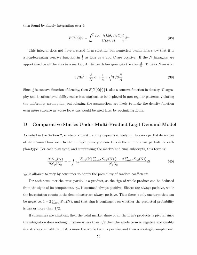
then found by simply integrating over θ:
E[U(d)|a] =
∫ π6
0
tan−1(L(θ, a)/C)
CL(θ, a)
6
πdθ (38)
This integral does not have a closed form solution, but numerical evaluations show that it is
a nondecreasing concave function in 1a as long as a and C are positive. If the N hexagons are
apportioned to all the area in a market, A, then each hexagon gets the area AN . Thus as N → +∞:
3√
3a2 =A
N⇐⇒ 1
a=
√3√
3N
A(39)
Since 1a is concave function of density, then E[U(d)|NA ] is also a concave function in density. Geogra-
phy and locations availability cause base stations to be deployed in non-regular patterns, violating
the uniformity assumption, but relaxing the assumptions are likely to make the density function
even more concave as worse locations would be used later by optimizing firms.
D Comparative Statics Under Multi-Product Logit Demand Model
As noted in the Section 2, strategic substitutability depends entirely on the cross partial derivative
of the demand function. In the multiple plan-type case this is the sum of cross partials for each
plan-type. For each plan type, and suppressing the market and time subscripts, this term is:
∂2Djk(N)
∂Nk∂Nn= −
∫γik
Sijk(N)∑
l∈J Silk′(N)(1− 2
∑l∈J Silk(N)
)NkNh
di (40)
γik is allowed to vary by consumer to admit the possibility of random coefficients.
For each consumer the cross partial is a product, so the sign of whole product can be deduced
from the signs of its components. γik is assumed always positive. Shares are always positive, while
the base station counts in the denominator are always positive. Thus there is only one term that can
be negative, 1 − 2∑
l∈J Silk(N), and that sign is contingent on whether the predicted probability
is less or more than 1/2.
If consumers are identical, then the total market share of all the firm’s products is pivotal since
the integration does nothing. If share is less than 1/2 then the whole term is negative and quality
is a strategic substitute; if it is more the whole term is positive and then a strategic complement.
56
If consumers differ, either because of consumer heterogeneity or random coefficients, then it is
ambiguous. For example, let’s say there are rich and poor consumers, and k has almost a pure
monopoly on rich consumers but sells almost nothing to poor consumers. Rich consumers are also a
minority, being less than 1/2. In aggregate, the poor consumers add almost nothing to the overall
derivative, but the rich consumers add very large positive amounts, so overall the derivative is
positive. Thus there could be strategic complements in quality with less than 1/2 market share.
57

E Tables and Figures
Table 1: Primary Reason for Switching Carriers
Percent of Survey Respondents
Primary Reason for Choosing Carrier Oct-Nov 2006 Feb-Mar 2008
Better Coverage 27% 22%Lower Prices 14% 19%
Family/Friends Subscribe to Carrier 13% 17%Plan Features 9% 12%
Promotional Offer 8% 9%Better Minute Level Plan 9% 7%
For a Specific Phone 4% 3%Other Reason 16% 11%
Taken directly from Comscore Wireless Report, Press Release March 31, 2008.See http://www.comscore.com/Insights/Press Releases/2008/03/Price Increasingly Important Factor in Cell Phone Carrier.
58
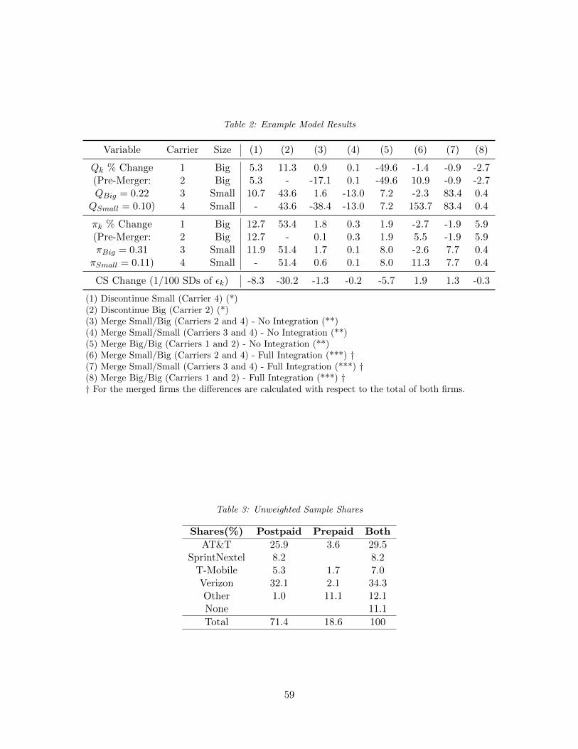
Table 2: Example Model Results
Variable Carrier Size (1) (2) (3) (4) (5) (6) (7) (8)
Qk % Change 1 Big 5.3 11.3 0.9 0.1 -49.6 -1.4 -0.9 -2.7(Pre-Merger: 2 Big 5.3 - -17.1 0.1 -49.6 10.9 -0.9 -2.7QBig = 0.22 3 Small 10.7 43.6 1.6 -13.0 7.2 -2.3 83.4 0.4QSmall = 0.10) 4 Small - 43.6 -38.4 -13.0 7.2 153.7 83.4 0.4
πk % Change 1 Big 12.7 53.4 1.8 0.3 1.9 -2.7 -1.9 5.9(Pre-Merger: 2 Big 12.7 - 0.1 0.3 1.9 5.5 -1.9 5.9πBig = 0.31 3 Small 11.9 51.4 1.7 0.1 8.0 -2.6 7.7 0.4πSmall = 0.11) 4 Small - 51.4 0.6 0.1 8.0 11.3 7.7 0.4
CS Change (1/100 SDs of εk) -8.3 -30.2 -1.3 -0.2 -5.7 1.9 1.3 -0.3
(1) Discontinue Small (Carrier 4) (*)(2) Discontinue Big (Carrier 2) (*)(3) Merge Small/Big (Carriers 2 and 4) - No Integration (**)(4) Merge Small/Small (Carriers 3 and 4) - No Integration (**)(5) Merge Big/Big (Carriers 1 and 2) - No Integration (**)(6) Merge Small/Big (Carriers 2 and 4) - Full Integration (***) †(7) Merge Small/Small (Carriers 3 and 4) - Full Integration (***) †(8) Merge Big/Big (Carriers 1 and 2) - Full Integration (***) †† For the merged firms the differences are calculated with respect to the total of both firms.
Table 3: Unweighted Sample Shares
Shares(%) Postpaid Prepaid Both
AT&T 25.9 3.6 29.5SprintNextel 8.2 8.2
T-Mobile 5.3 1.7 7.0Verizon 32.1 2.1 34.3Other 1.0 11.1 12.1None 11.1
Total 71.4 18.6 100
59

Fig
ure
5:
2000
PU
MA
s-
Su
bdiv
ided
into
Blo
ckG
rou
ps
Colo
red
by2010
Popu
lati
on
Den
sity
19
2
10
11
13
18
4
2212
21
75
14
23
16
6
3
15
23
17
8
19
25
20
24
60

Table 4: Unweighted Demographics in Sample and 2008-2012 American Community Survey
Income Sample(%) ACS(%) Age Sample(%) ACS(%)
Less than $35k 21.81 25.62 Teenagers† 6.27 5.20$35k-50k 12.16 11.02 18-34 Years 17.43 25.77$50-75k 21.95 16.69 35-64 Years 60.98 51.52
$75k-100k 17.20 13.38 65+ Years 15.32 17.51$100k+ 26.98 33.28
Household Size Sample(%) ACS(%) Sex Sample(%) ACS(%)
Single 18.54 27.41 Male 43.37 48.69Family 81.46 72.59 Female 56.63 51.31
Respondents to the Nielsen survey do not always answer all demographic questions. Respondents maydecline to reveal their income and 13% of respondents do so. Some Non-English speaking households(0.5%) are surveyed via phone interview instead of the usually online survey and information aboutincome and household size is sometimes not collected. Minors are not asked about their householdincome or household size (6%). Nielsen percentages are therefore calculated with respect to thepopulation for which answers are available.† The ACS does not report the teenaged population of states, while Nielsen does not sample anyoneunder 13 years old. Therefore reported ACS teenage percentage reflects the population of 10-17 yearolds.
Table 5: Count and Density of Base Stations by Market
Carrier Type Mean SD Min 25pct Median 75pct Max
Count AT&T 32.7 15.1 11 18 35 41 69Sprint 26.7 12.0 12 19 23.5 30 67
T-Mobile 25.5 12.3 10 19 25.5 32 79Verizon 25.3 12.8 5 17 22 34 58
All 27.9 13.4 5 18 24 36 79
Per 1000 km2 AT&T 1.22 1.06 0.17 0.67 0.87 1.40 5.11Sprint 1.16 1.18 0.20 0.48 0.71 1.24 4.52
T-Mobile 1.20 1.22 0.11 0.42 0.74 1.47 5.79Verizon 0.97 0.96 0.20 0.42 0.62 0.95 4.67
All 1.14 1.11 0.10 0.46 0.75 1.32 5.79
Table 6: Individual Level Identified Coefficients from MLE
Pure Logit MLE Nested Logit MLE † RC Logit MLE
β (KM to Store) -0.003 -0.003 -0.003(0.005) (0.005) (0.005)
λ( Nest Parameter) 1.09(0.13)
σ(S.D. of Rand. Co.) 0.08(0.16)
Observations 17,235 17,235 17,235Log Likelihood 29,607 29,607 29,607
McFadden’s Pseudo-R2 0.254 0.254 0.254
***, **, * indicate 1%, 5% and 10% significance, respectively.† Nested logit estimates are divided by λ for comparison with other specifications.
61

Table 7: Hausman-McFadden Tests of Independence of Irrelevant Alternatives for the Demand Model
Carrier Removed T-Stat Deg. Free. 5% Crit. Val.
AT&T -118.90 836 904.37Sprint 7.43 891 961.55
T-Mobile -12.69 837 905.42Verizon 22.19 836 904.37Other -95.09 844 912.70
Reports Chi-Square test of difference between estimated param-eters and parameters estimated using data without 1) the prod-ucts from the removed firm and 2) all individuals who choosethe removed products.
Table 8: Prepaid-Carrier-Year Fixed Effects from Pure Logit
AT&T T-Mobile Verizon Other
2008 -2.23*** -1.26*** -3.42*** 2.76***(0.30) (0.39) (0.46) (0.61)
2009 -2.49*** -1.48*** -3.07*** 4.35***(0.29) (0.36) (0.35) (0.71)
2010 -2.25*** -2.44*** -2.48*** 3.70***(0.29) (0.61) (0.29) (0.60)
2011 -2.19*** -0.80** -2.87*** 1.92***(0.25) (0.36) (0.35) (0.36)
2012 -1.88*** -0.87** -2.61*** 2.56***(0.22) (0.34) (0.31) (0.41)
***, **, * indicate 1%, 5% and 10% significance, re-spectively.The above represents the difference in mean utility ofprepaid plans relative to postpaid plans, for women be-tween the ages of 35 and 64, in multiple-person house-holds(families) that earn from $50-75 thousand annu-ally.
62
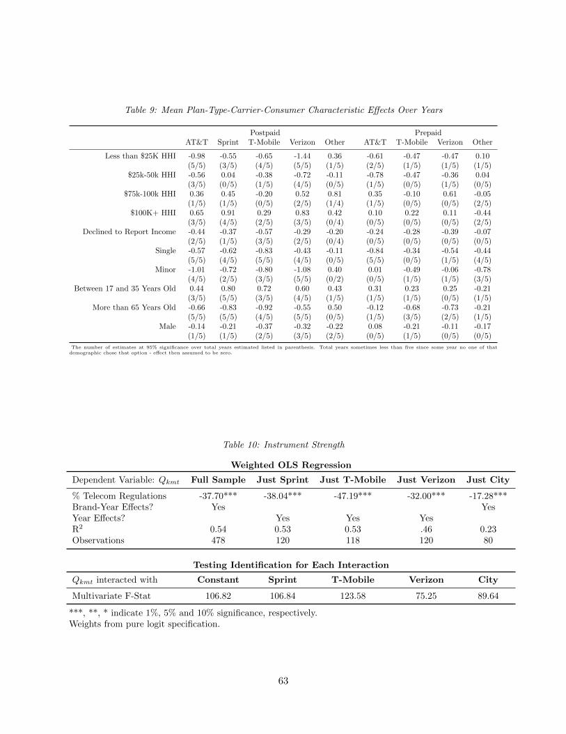
Table 9: Mean Plan-Type-Carrier-Consumer Characteristic Effects Over Years
Postpaid PrepaidAT&T Sprint T-Mobile Verizon Other AT&T T-Mobile Verizon Other
Less than $25K HHI -0.98 -0.55 -0.65 -1.44 0.36 -0.61 -0.47 -0.47 0.10(5/5) (3/5) (4/5) (5/5) (1/5) (2/5) (1/5) (1/5) (1/5)
$25k-50k HHI -0.56 0.04 -0.38 -0.72 -0.11 -0.78 -0.47 -0.36 0.04(3/5) (0/5) (1/5) (4/5) (0/5) (1/5) (0/5) (1/5) (0/5)
$75k-100k HHI 0.36 0.45 -0.20 0.52 0.81 0.35 -0.10 0.61 -0.05(1/5) (1/5) (0/5) (2/5) (1/4) (1/5) (0/5) (0/5) (2/5)
$100K+ HHI 0.65 0.91 0.29 0.83 0.42 0.10 0.22 0.11 -0.44(3/5) (4/5) (2/5) (3/5) (0/4) (0/5) (0/5) (0/5) (2/5)
Declined to Report Income -0.44 -0.37 -0.57 -0.29 -0.20 -0.24 -0.28 -0.39 -0.07(2/5) (1/5) (3/5) (2/5) (0/4) (0/5) (0/5) (0/5) (0/5)
Single -0.57 -0.62 -0.83 -0.43 -0.11 -0.84 -0.34 -0.54 -0.44(5/5) (4/5) (5/5) (4/5) (0/5) (5/5) (0/5) (1/5) (4/5)
Minor -1.01 -0.72 -0.80 -1.08 0.40 0.01 -0.49 -0.06 -0.78(4/5) (2/5) (3/5) (5/5) (0/2) (0/5) (1/5) (1/5) (3/5)
Between 17 and 35 Years Old 0.44 0.80 0.72 0.60 0.43 0.31 0.23 0.25 -0.21(3/5) (5/5) (3/5) (4/5) (1/5) (1/5) (1/5) (0/5) (1/5)
More than 65 Years Old -0.66 -0.83 -0.92 -0.55 0.50 -0.12 -0.68 -0.73 -0.21(5/5) (5/5) (4/5) (5/5) (0/5) (1/5) (3/5) (2/5) (1/5)
Male -0.14 -0.21 -0.37 -0.32 -0.22 0.08 -0.21 -0.11 -0.17(1/5) (1/5) (2/5) (3/5) (2/5) (0/5) (1/5) (0/5) (0/5)
The number of estimates at 95% significance over total years estimated listed in parenthesis. Total years sometimes less than five since some year no one of thatdemographic chose that option - effect then assumed to be zero.
Table 10: Instrument Strength
Weighted OLS Regression
Dependent Variable: Qkmt Full Sample Just Sprint Just T-Mobile Just Verizon Just City
% Telecom Regulations -37.70*** -38.04*** -47.19*** -32.00*** -17.28***Brand-Year Effects? Yes YesYear Effects? Yes Yes YesR2 0.54 0.53 0.53 .46 0.23Observations 478 120 118 120 80
Testing Identification for Each Interaction
Qkmt interacted with Constant Sprint T-Mobile Verizon City
Multivariate F-Stat 106.82 106.84 123.58 75.25 89.64
***, **, * indicate 1%, 5% and 10% significance, respectively.Weights from pure logit specification.
63
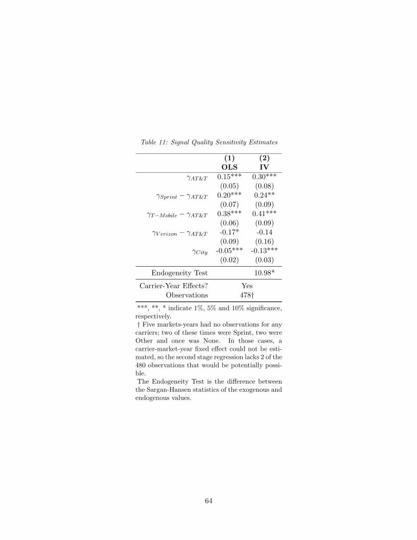
Table 11: Signal Quality Sensitivity Estimates
(1) (2)OLS IV
γAT&T 0.15*** 0.30***(0.05) (0.08)
γSprint − γAT&T 0.20*** 0.24**(0.07) (0.09)
γT−Mobile − γAT&T 0.38*** 0.41***(0.06) (0.09)
γV erizon − γAT&T -0.17* -0.14(0.09) (0.16)
γCity -0.05*** -0.13***(0.02) (0.03)
Endogeneity Test 10.98*
Carrier-Year Effects? YesObservations 478†
***, **, * indicate 1%, 5% and 10% significance,respectively.† Five markets-years had no observations for anycarriers; two of these times were Sprint, two wereOther and once was None. In those cases, acarrier-market-year fixed effect could not be esti-mated, so the second stage regression lacks 2 of the480 observations that would be potentially possi-ble.The Endogeneity Test is the difference betweenthe Sargan-Hansen statistics of the exogenous andendogenous values.
64

Table 12: Postpaid-Carrier-Year Fixed Effects from Pure Logit
η AT&T Sprint T-Mobile Verizon
2008 -0.085 -2.15*** -2.96*** 0.93(0.30) (0.36) (0.33) (0.67)
2009 -0.27 -2.23*** -2.67*** 1.21(0.32) (0.38) (0.33) (0.67)
2010 0.13 -2.23*** -3.20*** 0.88(0.33) (0.37) (0.38) (0.68)
2011 -0.03 -2.29*** -3.28*** 0.77(0.32) (0.39) (0.37) (0.71)
2012 0.00 -2.23*** -2.97*** 0.76(0.33) (0.39) (0.36) (0.72)
***, **, * indicate 1%, 5% and 10% significance, re-spectively.The above represents the mean utility of postpaidplans net of signal quality, for women between the agesof 35 and 64, in multiple-person households(families)that earn from $50-75 thousand annually.
Table 13: Median Quality Elasticities for Instrumented Pure Logit Specification
1% Change in Signal Quality Proxy of...Full Sample AT&T Sprint T-Mobile Verizon
...Results AT&T 0.25 -0.06 -0.06 -0.06in Change Sprint -0.03 0.16 -0.02 -0.02of Market T-Mobile -0.03 -0.01 0.18 -0.01
Share % of... Verizon -0.13 -0.06 -0.06 0.13
1% Change in Signal Quality Proxy of...2012 AT&T Sprint T-Mobile Verizon
...Results AT&T 0.27 -0.05 -0.04 -0.06in Change Sprint -0.03 0.15 -0.01 -0.01of Market T-Mobile -0.02 -0.01 0.16 -0.01
Share % of... Verizon -0.12 -0.06 -0.06 0.13
Matrices do not represent any particular market. Rather, each entry is the median acrossmarket-years for that particular firm.
65

Table 14: Correlation in Mean Utility Attributable to Only Demographics and Years
AT&T Sprint T-Mobile Verizon OtherPre Post Post Pre Post Pre Post Pre Post
AT&T Pre 1.00 - - - - - - - -Post 0.72 1.00 - - - - - - -
Sprint Pre 0.58 0.91 1.00 - - - - - -T-Mobile Pre 0.45 0.66 0.69 1.00 - - - - -
Post 0.53 0.81 0.87 0.64 1.00 - - - -Verizon Pre 0.63 0.69 0.59 0.41 0.58 1.00 - - -
Post 0.69 0.96 0.88 0.61 0.76 0.62 1.00 - -Other Pre -0.17 -0.06 0.01 -0.02 0.01 -0.14 0.10 1.00 -
Post -0.03 0.02 0.07 0.01 -0.03 -0.23 0.02 0.58 1.00
This table displays the correlation of the difference between the estimated product utility for a consumer and thebrand-market utility, δijkt − ξkmt, for the Nielsen sample.
Table 15: Marginal Base Station Cost - Fkmt ($1000)
Full Sample
Carrier Mean SD Min 25pct Median 75pct Max
AT&T 11.8 3.7 4.8 8.8 11.6 11.6 22.3Sprint 8.6 3.6 2.4 5.5 8.2 11.0 21.1
T-Mobile 8.5 5.5 0.2 4.5 7.4 11.2 29.5Verizon 7.1 3.3 0.8 4.6 7.0 9.2 15.1
2012
Carrier Mean SD Min 25pct Median 75pct Max
AT&T 12.5 3.6 6.5 9.3 12.4 15.4 18.5Sprint 9.3 4.5 3.2 5.5 8.0 11.7 21.1
T-Mobile 6.9 3.5 0.8 4.3 6.4 8.9 16.6Verizon 6.9 3.2 0.9 5.0 6.6 8.9 14.0
Table 16: Total CT Costs as % of Variable Profit by Year
Year AT&T Sprint T-Mobile Verizon
2008 19.26 44.76 58.90 8.902009 18.85 45.56 59.20 8.932010 19.05 46.45 59.87 9.282011 18.67 44.86 61.71 8.812012 18.96 45.57 61.87 9.19
66
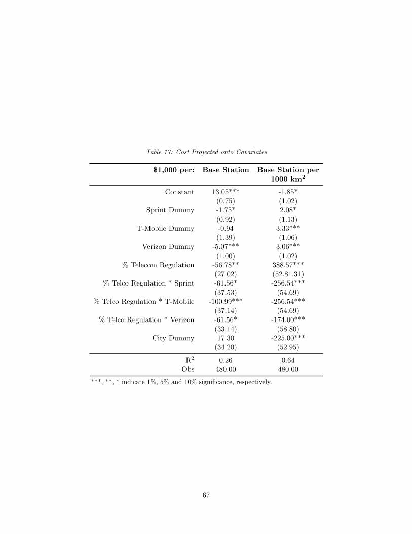
Table 17: Cost Projected onto Covariates
$1,000 per: Base Station Base Station per1000 km2
Constant 13.05*** -1.85*(0.75) (1.02)
Sprint Dummy -1.75* 2.08*(0.92) (1.13)
T-Mobile Dummy -0.94 3.33***(1.39) (1.06)
Verizon Dummy -5.07*** 3.06***(1.00) (1.02)
% Telecom Regulation -56.78** 388.57***(27.02) (52.81.31)
% Telco Regulation * Sprint -61.56* -256.54***(37.53) (54.69)
% Telco Regulation * T-Mobile -100.99*** -256.54***(37.14) (54.69)
% Telco Regulation * Verizon -61.56* -174.00***(33.14) (58.80)
City Dummy 17.30 -225.00***(34.20) (52.95)
R2 0.26 0.64Obs 480.00 480.00
***, **, * indicate 1%, 5% and 10% significance, respectively.
67
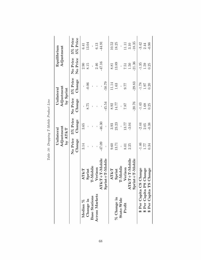
Tabl
e18:
Dro
ppin
gT
-Mo
bile
Pro
du
ctL
ine
Un
ilate
ral
Un
ilate
ral
Equ
ilib
riu
mA
dju
stm
ent
Ad
just
ment
Ad
just
ment
by
AT
&T
by
Sp
rint
No
Pri
ce
5%
Pri
ce
No
Pri
ce
5%
Pri
ce
No
Pri
ce
5%
Pri
ce
Ch
an
ge
Ch
an
ge
Ch
an
ge
Ch
an
ge
No
Pri
ce
5%
Pri
ce
Med
ian
%A
T&
T3.
143.
65-
-2.
906.
41C
han
ge
inS
pri
nt
--
8.75
-0.0
68.
1513
.04
Base
Sta
tion
sT
-Mob
ile
--
--
--
Acro
ssM
ark
ets
Veri
zon
--
--
2.46
6.13
AT
&T
+T
-Mob
ile
-47.
09-4
6.30
--
-47.
16-4
4.91
Sp
rint+
T-M
ob
ile
--
-45.
54-5
0.79
AT
&T
9.60
3.93
8.92
11.1
48.
8110
.52
%C
han
ge
inS
pri
nt
13.7
123
.23
14.7
71.
6313
.89
18.2
5S
tate
-Wid
eT
-Mob
ile
--
--
--
Pro
fit
Veri
zon
8.01
13.7
77.
879.
777.
5111
.11
AT
&T
+T
-Mob
ile
2.25
-3.0
41.
503.
10S
pri
nt+
T-M
ob
ile
-20.
76-2
9.83
-21.
36-1
8.35
$P
er
Cap
ita
CS
Ch
an
ge
-1.4
6-2
.44
-1.4
3-1
.78
-1.3
5-3
.42
$P
er
Cap
ita
PS
Ch
an
ge
1.77
2.05
1.68
1.97
1.59
2.44
$P
er
Cap
ita
TS
Ch
an
ge
0.34
-0.3
80.
250.
200.
25-0
.98
68
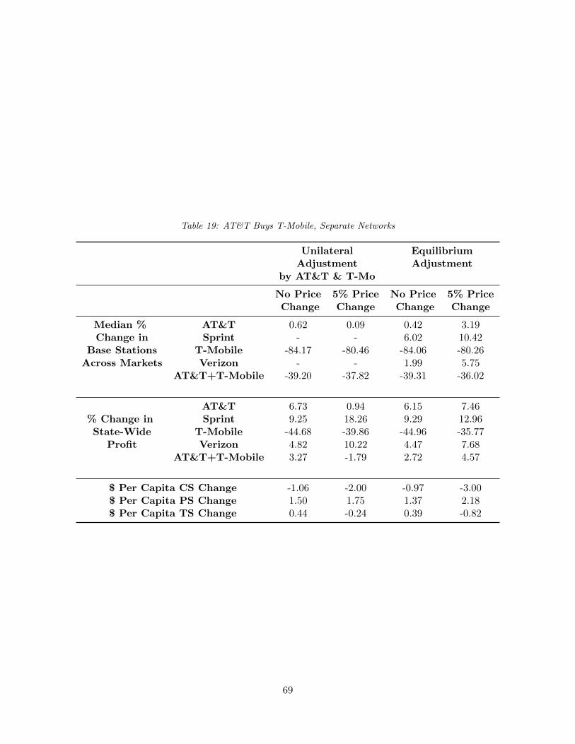
Table 19: AT&T Buys T-Mobile, Separate Networks
Unilateral EquilibriumAdjustment Adjustment
by AT&T & T-Mo
No Price 5% Price No Price 5% PriceChange Change Change Change
Median % AT&T 0.62 0.09 0.42 3.19Change in Sprint - - 6.02 10.42
Base Stations T-Mobile -84.17 -80.46 -84.06 -80.26Across Markets Verizon - - 1.99 5.75
AT&T+T-Mobile -39.20 -37.82 -39.31 -36.02
AT&T 6.73 0.94 6.15 7.46% Change in Sprint 9.25 18.26 9.29 12.96State-Wide T-Mobile -44.68 -39.86 -44.96 -35.77
Profit Verizon 4.82 10.22 4.47 7.68AT&T+T-Mobile 3.27 -1.79 2.72 4.57
$ Per Capita CS Change -1.06 -2.00 -0.97 -3.00$ Per Capita PS Change 1.50 1.75 1.37 2.18$ Per Capita TS Change 0.44 -0.24 0.39 -0.82
69

Table 20: Sprint Buys T-Mobile, Separate Networks
Unilateral EquilibriumAdjustment Adjustment
by Sprint & T-Mo
No Price 5% Price No Price 5% PriceChange Change Change Change
Median % AT&T - - 0.69 3.89Change in Sprint -4.98 -13.29 -4.93 -1.66
Base Stations T-Mobile -27.63 -30.91 -27.74 -18.56Across Markets Verizon - - 0.69 4.62
Sprint+T-Mobile -15.61 -22.14 -15.56 -10.23
AT&T 1.83 4.61 1.81 2.93% Change in Sprint 2.63 -8.25 2.45 5.72State-Wide T-Mobile -2.24 -11.00 -2.48 9.00
Profit Verizon 1.54 3.96 1.48 4.46Sprint+T-Mobile 1.12 -9.10 0.92 6.73
$ Per Capita CS Change -0.31 -0.76 -0.29 -2.30$ Per Capita PS Change 0.50 0.90 0.48 1.24$ Per Capita TS Change 0.19 -0.14 0.19 -1.06
70

Table 21: AT&T Buys T-Mobile, Single Network, AT&T Costs
Unilateral EquilibriumAdjustment Adjustment
by AT&T & T-Mo
No Price 5% Price No Price 5% PriceChange Change Change Change
Median % AT&T 26.49 29.77 26.67 33.11Change in Sprint - - -5.02 -1.73
Base Stations T-Mobile 37.84 40.86 38.03 43.93Across Markets† Verizon - - -1.50 2.47
AT&T+T-Mobile -34.96 -33.98 -34.91 -32.03
AT&T - - - -% Change in Sprint -6.91 2.26 -6.72 -3.61State-Wide T-Mobile - - - -
Profit†† Verizon -4.19 1.32 -3.97 -1.09AT&T+T-Mobile 11.67 7.29 12.08 14.70
$ Per Capita CS Change 0.78 -0.26 0.72 -1.30$ Per Capita PS Change 0.91 1.27 1.00 1.86$ Per Capita TS Change 1.69 1.01 1.73 0.55
† For the merged firms the final base station count used for the difference is the effective count, whichsum of the count of the two merging firms.†† For the merged firms cost cannot be disentangled between the two networks so for those firms I donot report individual profits.
71

Table 22: AT&T Buys T-Mobile, Single Network, T-Mobile Costs
Unilateral EquilibriumAdjustment Adjustment
by AT&T & T-Mo
No Price 5% Price No Price 5% PriceChange Change Change Change
Median % AT&T 159.45 168.02 160.38 174.40Change in Sprint - - -22.66 -19.90
Base Stations T-Mobile 251.21 264.24 251.43 270.55Across Markets† Verizon - - -7.06 -3.36
AT&T+T-Mobile 43.22 49.02 43.46 51.19
AT&T - - - -% Change in Sprint -26.28 -17.45 -24.24 -21.79State-Wide T-Mobile - - - -
Profit†† Verizon -15.84 -10.55 -15.04 -12.54AT&T+T-Mobile 30.04 26.51 31.99 35.62
$ Per Capita CS Change 3.25 2.12 3.01 0.98$ Per Capita PS Change 1.43 1.88 1.87 2.80$ Per Capita TS Change 4.68 4.00 4.88 3.78
† For the merged firms the final base station count used for the difference is the effective count, whichsum of the count of the two merging firms.†† For the merged firms cost cannot be disentangled between the two networks so for those firms I donot report individual profits.
72
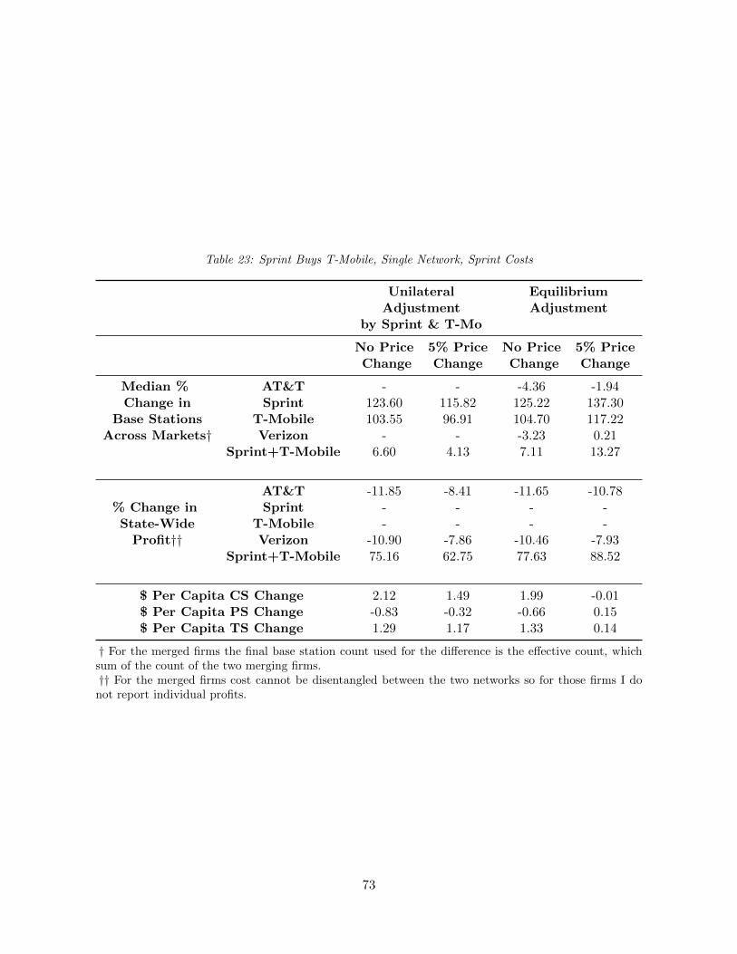
Table 23: Sprint Buys T-Mobile, Single Network, Sprint Costs
Unilateral EquilibriumAdjustment Adjustment
by Sprint & T-Mo
No Price 5% Price No Price 5% PriceChange Change Change Change
Median % AT&T - - -4.36 -1.94Change in Sprint 123.60 115.82 125.22 137.30
Base Stations T-Mobile 103.55 96.91 104.70 117.22Across Markets† Verizon - - -3.23 0.21
Sprint+T-Mobile 6.60 4.13 7.11 13.27
AT&T -11.85 -8.41 -11.65 -10.78% Change in Sprint - - - -State-Wide T-Mobile - - - -
Profit†† Verizon -10.90 -7.86 -10.46 -7.93Sprint+T-Mobile 75.16 62.75 77.63 88.52
$ Per Capita CS Change 2.12 1.49 1.99 -0.01$ Per Capita PS Change -0.83 -0.32 -0.66 0.15$ Per Capita TS Change 1.29 1.17 1.33 0.14
† For the merged firms the final base station count used for the difference is the effective count, whichsum of the count of the two merging firms.†† For the merged firms cost cannot be disentangled between the two networks so for those firms I donot report individual profits.
73

Table 24: Sprint Buys T-Mobile, Single Network, T-Mobile Costs
Unilateral EquilibriumAdjustment Adjustment
by Sprint & T-Mo
No Price 5% Price No Price 5% PriceChange Change Change Change
Median % AT&T - - -8.48 -6.76Change in Sprint 229.24 221.89 232.46 253.73
Base Stations T-Mobile 284.76 276.12 288.63 311.64Across Markets† Verizon - - -6.42 -2.95
Sprint+T-Mobile 69.88 65.31 71.44 82.64
AT&T -16.84 -13.20 -16.54 -15.74% Change in Sprint - - - -State-Wide T-Mobile - - - -
Profit †† Verizon -14.10 -10.90 -13.53 -11.09Sprint+T-Mobile 109.68 96.76 113.56 126.27
$ Per Capita CS Change 3.00 2.30 2.83 0.82$ Per Capita PS Change -0.89 -0.32 -0.65 0.20$ Per Capita TS Change 2.11 1.96 2.18 1.02
† For the merged firms the final base station count used for the difference is the effective count, whichsum of the count of the two merging firms.†† For the merged firms cost cannot be disentangled between the two networks so for those firms I donot report individual profits.
74