qualitatively characterizing neural network … characterizing neural network optimization ... there...

Qualitatively Characterizing Neural Network Optimization

Problems

1

Ian Goodfellow Oriol Vinyals Andrew Saxe

2015 International Conference on Representation Learning --- Goodfellow, Vinyals, and Saxe 2

Traditional view of NN training


Factored linear view(Cartoon of

Saxe et al 2013’sworldview)


Attractive saddle point view(Cartoon of

Dauphin et al 2014’sworldview)

2015 International Conference on Representation Learning --- Goodfellow, Vinyals, and Saxe

• Does SGD get stuck in local minima?• Does SGD get stuck on saddle points?• Does SGD wind around numerous bumpy

obstacles?• Does SGD thread a twisting canyon?

5

Questions


• Visualize trajectories of (near) SOTA results• Selection bias: looking at success• Failure is interesting, but hard to attribute to

optimization• Careful with interpretation

• SGD never encounters X?• SGD fails if it encounters X?

6

History written by the winners


2-D subspace visualization

7

Cost

Projection 1 Projection 0


A special 1-D subspace

8

Interpolation plot

Learning curve


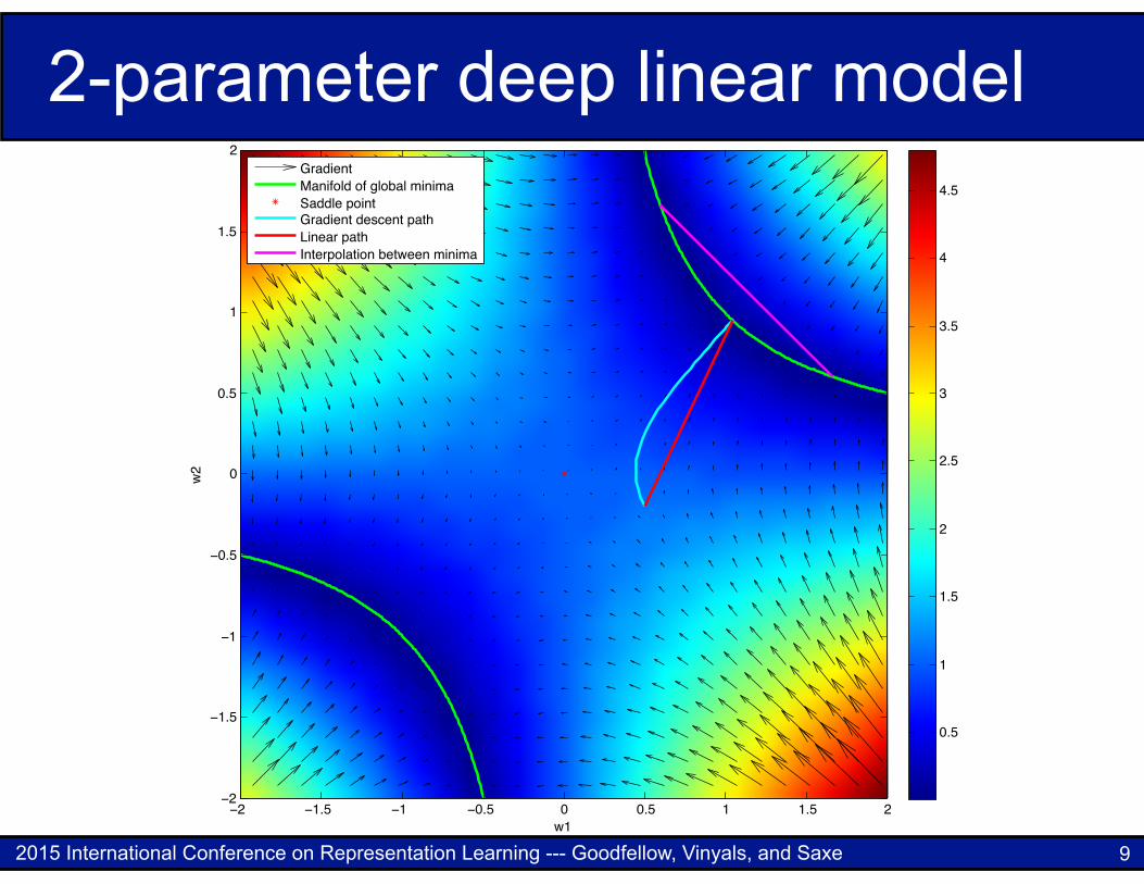
2-parameter deep linear model

9w1

w2

−2 −1.5 −1 −0.5 0 0.5 1 1.5 2−2

−1.5

−1

−0.5

0

0.5

1

1.5

2GradientManifold of global minimaSaddle pointGradient descent pathLinear pathInterpolation between minima

0.5

1

1.5

2

2.5

3

3.5

4

4.5

Student Version of MATLAB


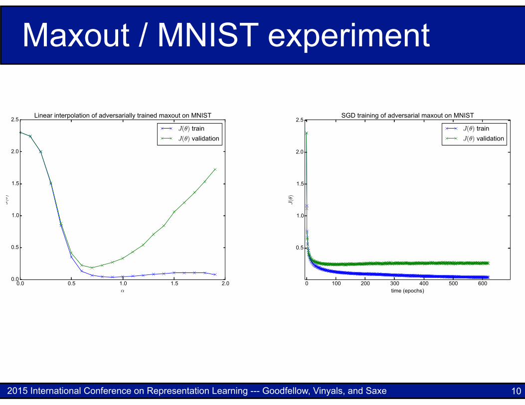
Maxout / MNIST experiment

10

Published as a conference paper at ICLR 2015

Figure 1: Experiments with maxout on MNIST. Top row) The state of the art model, with adver-sarial training. Bottom row) The previous best maxout network, without adversarial training. Leftcolumn) The linear interpolation experiment. This experiment shows that the objective function isfairly smooth within the 1-D subspace spanning the initial and final parameters of the model. Apartfrom the flattening near ↵ = 0, it appears nearly convex in this subspace. If we chose the initialdirection correctly, we could solve the problem with a coarse line search. Local optima and barrierssuch as ridges in the objective function do not appear to be a problem, nor does it appear that thenetwork needs to thread a narrow and winding ravine. Right column) The progress of the actualSGD algorithm over time. The vast majority of learning happens in the first few epochs. Thereafter,the algorithm struggles to make progress. The lack of progress does not appear to be due to movingaround obstacles. Instead, it may be due to a less exotic optimization difficulty, such as noise in theestimate of the gradient, or poor conditioning.

Figure 2: The linear interpolation curves for fully connected networks with different activationfunctions. Left) Sigmoid activation function. Right) ReLU activation function.

3


Other activation functions

11


Figure 1: Experiments with maxout on MNIST. Top row) The state of the art model, with adver-sarial training. Bottom row) The previous best maxout network, without adversarial training. Leftcolumn) The linear interpolation experiment. This experiment shows that the objective function isfairly smooth within the 1-D subspace spanning the initial and final parameters of the model. Apartfrom the flattening near ↵ = 0, it appears nearly convex in this subspace. If we chose the initialdirection correctly, we could solve the problem with a coarse line search. Local optima and barrierssuch as ridges in the objective function do not appear to be a problem, nor does it appear that thenetwork needs to thread a narrow and winding ravine. Right column) The progress of the actualSGD algorithm over time. The vast majority of learning happens in the first few epochs. Thereafter,the algorithm struggles to make progress. The lack of progress does not appear to be due to movingaround obstacles. Instead, it may be due to a less exotic optimization difficulty, such as noise in theestimate of the gradient, or poor conditioning.

Figure 2: The linear interpolation curves for fully connected networks with different activationfunctions. Left) Sigmoid activation function. Right) ReLU activation function.

3


Convolutional network

12


Figure 5: Here we use linear interpolation to search for local minima. Left) By interpolating betweentwo different SGD solutions, we show that each solution is a different local minimum within this1-D subspace. Right) If we interpolate between a random point in space and an SGD solution, wefind no local minima besides the SGD solution, suggesting that local minima are rare.

Figure 6: The linear interpolation experiment for a convolutional maxout network on the CIFAR-10dataset (Krizhevsky & Hinton, 2009). Left) At a global scale, the curve looks very well-behaved.Right) Zoomed in near the initial point, we see there is a shallow barrier that SGD must navigate.

There are of course multiple minima in neural network optimization problems, and the shortest pathbetween two minima can contain a barrier of higher cost. We can find two different solutions by us-ing different random seeds for the random number generators used to initialize the weights, generatedropout masks, and select examples for SGD minibatches. (It is possible that these solutions are notminima but saddle points that SGD failed to escape) We do not find any local minima within thissubspace other than solution points, and these different solutions appear to correspond to differentchoices of how to break the symmetry of the saddle point at the origin, rather than to fundamentallydifferent solutions of varying quality. See Fig. 5.

4 ADVANCED NETWORKS

Having performed experiments to understand the behavior of neural network optimization on su-pervised feedforward networks, we now verify that the same behavior occurs for more advancednetworks.

In the case of convolutional networks, we find that there is a single barrier in the objective function,near where the network is initialized. This may simply correspond to the network being initializedwith too large of random weights. This barrier is reasonably wide but not very tall. See Fig. 6 fordetails.

To examine the behavior of SGD on generative models, we experimented with an MP-DBM (Good-fellow et al., 2013a). This model is useful for our purposes because it gets good performance asa generative model and as a classifier, and its objective function is easy to evaluate (no MCMCbusiness). Here we find a secondary local minimum with high error, but a visualization of the SGDtrajectory reveals that SGD passed far enough around the anomaly to avoid having it affect learn-

5


Figure 5: Here we use linear interpolation to search for local minima. Left) By interpolating betweentwo different SGD solutions, we show that each solution is a different local minimum within this1-D subspace. Right) If we interpolate between a random point in space and an SGD solution, wefind no local minima besides the SGD solution, suggesting that local minima are rare.

Figure 6: The linear interpolation experiment for a convolutional maxout network on the CIFAR-10dataset (Krizhevsky & Hinton, 2009). Left) At a global scale, the curve looks very well-behaved.Right) Zoomed in near the initial point, we see there is a shallow barrier that SGD must navigate.

There are of course multiple minima in neural network optimization problems, and the shortest pathbetween two minima can contain a barrier of higher cost. We can find two different solutions by us-ing different random seeds for the random number generators used to initialize the weights, generatedropout masks, and select examples for SGD minibatches. (It is possible that these solutions are notminima but saddle points that SGD failed to escape) We do not find any local minima within thissubspace other than solution points, and these different solutions appear to correspond to differentchoices of how to break the symmetry of the saddle point at the origin, rather than to fundamentallydifferent solutions of varying quality. See Fig. 5.

4 ADVANCED NETWORKS

Having performed experiments to understand the behavior of neural network optimization on su-pervised feedforward networks, we now verify that the same behavior occurs for more advancednetworks.

In the case of convolutional networks, we find that there is a single barrier in the objective function,near where the network is initialized. This may simply correspond to the network being initializedwith too large of random weights. This barrier is reasonably wide but not very tall. See Fig. 6 fordetails.

To examine the behavior of SGD on generative models, we experimented with an MP-DBM (Good-fellow et al., 2013a). This model is useful for our purposes because it gets good performance asa generative model and as a classifier, and its objective function is easy to evaluate (no MCMCbusiness). Here we find a secondary local minimum with high error, but a visualization of the SGDtrajectory reveals that SGD passed far enough around the anomaly to avoid having it affect learn-

5

A small barrier


LSTM

13


Figure 7: Experiments with the MP-DBM. Left) The linear interpolation experiment reveals a sec-ondary local minimum with high error. Right) On the two horizonal axes, we plot components of✓ that capture the extrema of ✓ throughout the learning process. On the vertical axis, we plot theobjective function. Each point is another epoch of actual SGD learning. This plot allows us to seethat SGD did not pass near this anomaly.

Figure 8: The linear interpolation experiment for an LSTM trained on the Penn Treebank dataset.

ing. See Fig. 7. The MP-DBM was initialized with very large, sparse, weights, which may havecontributed to this model having more non-convex behavior than the others.

Finally, we performed the linear interpolation experiment for an LSTM regularized withdropout (Hochreiter & Schmidhuber, 1997; Zaremba et al., 2014) on the Penn Treebankdataset (Marcus et al., 1993). See Fig. 8. This experiment did not find any difficult structures,showing that the exotic features of non-convex optimization do not appear to cause difficulty evenfor recurrent models of sequences.

5 DEEP LINEAR NETWORKS

Saxe et al. (2013) have advocated developing a mathematical theory of deep networks by studyingsimplified mathematical models of these networks. Deep networks are formed by composing analternating series of learned affine transformations and fixed non-linearities. One simplified way tomodel these functions is to compose only a series of learned linear transformations. The compositionof a series of linear transformations is itself a linear transformation, so this mathematical model lacksthe expressive capacity of a general deep network. However, because the weights of such a modelare factored, its learning dynamics resemble those of the deep network. In particular, while linearregression is a convex problem, deep linear regression is a non-convex problem.

Deep linear regression suffers from saddle points but does not suffer from local minima of varyingquality. All minima are global minima, and are linked to each other in a continuous manifold.

Our linear interpolation experiments can be carried out analytically rather than experimentally in thecase of deep linear regression. The results are strikingly similar to our results with deep non-linearnetworks.

6


MP-DBM

14


Figure 7: Experiments with the MP-DBM. Left) The linear interpolation experiment reveals a sec-ondary local minimum with high error. Right) On the two horizonal axes, we plot components of✓ that capture the extrema of ✓ throughout the learning process. On the vertical axis, we plot theobjective function. Each point is another epoch of actual SGD learning. This plot allows us to seethat SGD did not pass near this anomaly.

Figure 8: The linear interpolation experiment for an LSTM trained on the Penn Treebank dataset.

ing. See Fig. 7. The MP-DBM was initialized with very large, sparse, weights, which may havecontributed to this model having more non-convex behavior than the others.

Finally, we performed the linear interpolation experiment for an LSTM regularized withdropout (Hochreiter & Schmidhuber, 1997; Zaremba et al., 2014) on the Penn Treebankdataset (Marcus et al., 1993). See Fig. 8. This experiment did not find any difficult structures,showing that the exotic features of non-convex optimization do not appear to cause difficulty evenfor recurrent models of sequences.

5 DEEP LINEAR NETWORKS

Saxe et al. (2013) have advocated developing a mathematical theory of deep networks by studyingsimplified mathematical models of these networks. Deep networks are formed by composing analternating series of learned affine transformations and fixed non-linearities. One simplified way tomodel these functions is to compose only a series of learned linear transformations. The compositionof a series of linear transformations is itself a linear transformation, so this mathematical model lacksthe expressive capacity of a general deep network. However, because the weights of such a modelare factored, its learning dynamics resemble those of the deep network. In particular, while linearregression is a convex problem, deep linear regression is a non-convex problem.

Deep linear regression suffers from saddle points but does not suffer from local minima of varyingquality. All minima are global minima, and are linked to each other in a continuous manifold.

Our linear interpolation experiments can be carried out analytically rather than experimentally in thecase of deep linear regression. The results are strikingly similar to our results with deep non-linearnetworks.

6


3-D Visualization

15


3-D MP-DBM visualization

16


Random walk control

17


Figure 11: Plots of the projection along the axis from initialization to solution versus the normof the residual of this projection for random walks of varying dimension. Each plot is formed byusing 1,000 steps. We designate step 900 as being the “solution” and continue to plot 100 moresteps, in order to simulate the way neural network training trajectories continue past the point thatearly stopping on a validation set criterion chooses as being the solution. Each step is made byincrementing the current coordinate by a sample from a Gaussian distribution with zero mean andunit covariance. Because the dimensionality of the space forces most trajectories to have this highlyregular shape, this kind of plot is not a meaningful way of investigating how SGD behaves as itmoves away from the 1-D subspace we study in this paper.

Stochastic gradient descent does not actually follow this path. We know that SGD matches this pathat the beginning and at the end.

One might naturally want to plot the norm of the residual of the parameter value after projectingthe parameters at each point in time into the 1-D subspace we have identified. However, it turnsout that in high dimensional spaces, the shape of this curve does not convey very much information.See Fig. 11 for a demonstration of how this plot converges to a simple geometric shape as thedimensionality of a random walk increases.

Plots of the residual norm of the projection for SGD trajectories converge to a very similar geometricshape in high dimensional spaces. See Fig. 12 for an example of several different runs of SGD onthe same problem. However, we can still glean some information from this kind of plot by lookingat the maximum norm of the residual and comparing this to the maximum norm of the parametervector as a whole.

We show this same kind of plot for a maxout network in Fig. 13. Keep in mind that the shape of thetrajectory is not interesting, but the ratio of the norm of the residual to the total norm of the parametervector at each point does give us some idea of how much information the 1-D projection discards.We see from this plot that our linear subspace captures at least 2/3 the norm of the parameter vectorat all points in time.

10


3-D Plots Without Obstacles

18

LSTM

AdversarialReLUs

Factored Linear


3-D Plot of Adversarial Maxout

19

SGD naturally exploitsnegative curvature!

Obstacles!


Conclusion

• For most problems, there exists a linear subspace of monotonically decreasing values

• For some problems, there are obstacles between this subspace the SGD path

• Factored linear models capture many qualitative aspects of deep network training

• See more visualizations at our poster / demo / paper

20

qualitatively characterizing neural network … characterizing neural network optimization ... there...

Documents