qualitative and quantitative formal model-based safety ... · acknowledgments i would like to...
TRANSCRIPT
Otto-von-Guericke-Universitat Magdeburg
Qualitative and Quantitative FormalModel-Based Safety Analysis
– Push the Safety Button –
Dissertationzur Erlangung des akademischen GradesDoktoringenieur (Dr.-Ing.)
angenommen durch die Fakultat fur Informatik
der Otto-von-Guericke-Universitat Magdeburg
von: Dipl.-Inf. Matthias Gudemann
geb. am 11.06.1980 in Augsburg
Gutachter: Jun.-Prof. Dr. Frank Ortmeier
Prof. Dr. Jean-Jacques LesageProf. Dr. Rudolf Kruse
Ort und Datum des Promotionskolloquiums: Magdeburg, 29.09.2011

Acknowledgments
I would like to express my gratitude to my advisor and colleague Jun.-Prof.Dr. Frank Ortmeier, whose expertise in the areas of safety analysis, formalmethods and mathematics and whose willingness to share his ideas and opin-ion in many discussions, contributed greatly to the successful completion ofmy dissertation thesis. I would like to thank Prof. Dr. Jean-Jacques Lesageand Prof. Dr. Rudolf Kruse for taking time from their busy schedule to serveas reviewers for my dissertation thesis.My special thanks go to Prof. Dr. Wolfgang Reif, who encouraged and sup-ported me from the very first semester of my university studies and continuedto do so throughout my academic career. I learned a lot at the time at hischair at the University of Augsburg and the opportunity to work with manystudents in lectures, seminars and different exercises provided me with veryvaluable experiences.I would also like to thank all my colleagues and now friends, both at Augsburgand Magdeburg for all the discussions, support and fun we had together – atthe workplace, as well as in the leisure time.My deepest gratitude goes to my family for the support they provided methrough my life, my parents who encouraged me to follow whatever I wantedto do and in particular to my partner Agnes for showing me so much I wouldnever have experienced without her.

Zusammenfassung
In vielen Anwendungsbereichen wird Software mehr und mehr zum Hauptin-novationsfaktor. Immer großere Teile der Funktionalitat von Systemen werdendurch Software implementiert, die auf generischer Hardware lauft. Dafur hatsich der Begriff der software-intensiven Systeme etabliert. Mittlerweile sindsolche Systeme auch in sicherheitskritischen Bereichen weit verbreitet. Mitihrer Verwendung geht eine enorme Erhohung der Komplexitat einher, welcheden Nachweis der funktionalen Sicherheit immer schwieriger macht. Einsolcher Nachweis ist in sicherheitskritischen Bereichen jedoch notwendig undwird von den entsprechenden Zertifizierungsstellen gefordert. Die genauen An-forderungen dafur sind in domanenspezifischen Normen und Standards spez-ifiziert.Die Verwendung formaler Methoden zur modellbasierten Sicherheitsanalysekann den Sicherheitsnachweis fur solche Systeme unterstutzen. Dazu wirdein gemeinsames formales Systemmodell erstellt, welches sich der Entwicklerund der Sicherheitsingenieur teilen. Dieses Modell besteht dabei aus einemabstrakten Modell des funktionalen Systems, einem Modell des physikalis-chen Umweltverhaltens, sowie einem Modell des Fehlverhaltens. Ein solchesModell kann in einer Sprache mit formaler Semantik ausgedruckt werden.Dies erlaubt dann eine Analyse mit automatischen Modellprufern und un-terstutzt so den Sicherheitsanalyseprozess fur komplexe Systeme. Der Vorteilgegenuber bisherigen Verfahren liegt dabei einmal in der Verwendung einesgemeinsamen Modells, was den notwendigen Aufwand bei Designanderungenverringert. Der zweite Vorteil liegt in der erhohten Automatisierung, wodurchein Sicherheitsnachweis effizienter durchgefuhrt werden kann.Die Ergebnisse dieser Dissertation verbessern die bisher existierenden mod-ellbasierten Analysemethoden wesentlich. Hauptaspekte dabei sind einmaldie Erweiterung der analysierbaren Systemklasse sowie die Erweiterung deranalysierbaren Eigenschaften. Desweiteren wurde eine neue, probabilistis-che Sicherheitsanalysemethodik geschaffen, die wesentlich genauere Ergeb-nisse liefern kann als dies mit bisherigen Analysen moglich war. Die Ba-sis dazu bildet die formale Beschreibungssprache SAML (Safety Analysisand Modeling Language). Fur diese wurde eine prototypische Werkzeugun-terstutzung geschaffen, die es erlaubt, SAML Modelle durch Modelltransfor-mationen mit verschiedenen Verifikationstools zu analysieren. Dadurch profi-tiert der Ansatz von jeder Erweiterung der unterstutzten Analysetools. DieserAnsatz erlaubt eine Kombination verschiedener Analysemethoden und bildetdie Basis fur eine toolunabhangige Analyseplattform. Der Ansatz wird mitder Analyse von drei Fallstudien illustriert und bildet die Basis fur das DFGEinzelforschungsprojekt “ProMoSA” (Probabilistic Models for Safety Analy-sis).
5


Abstract
Software is becoming the main innovation factor in many domains. Everymore functionality is implemented in software running on relatively generichardware. For this the notion of software-intensive systems has been estab-lished. By now such systems are already common in safety-critical domains.Their application causes an increase of complexity which makes the assuranceof functional safety ever harder. Such evidence of safety is required in safety-critical domains and is required by the responsible certification authorities.The exact requirements are specified in domain-specific standards.Using formal methods for model-based safety analysis can support the safetyassurance of such systems. The basis is the construction of a common formalsystem model which is shared between the developer and the safety engineer.Such a model generally consists of an abstract model of the system, a model ofthe physical behavior of the environment and a model of the possible faults andfailure modes. A model expressed in a language with formal semantics allowsfor the analysis using automatic verification tools and can therefore supportthe safety analysis process of complex systems. Compared to more traditionalapproaches the advantages are firstly that using a common system modelrequires less effort in case of design changes and secondly in the increasedautomation which make more efficient safety analysis possible.The results of this dissertation thesis significantly advance existing safety anal-ysis methods. Firstly, the class of analyzable systems is extended and secondlythe set of analyzable properties is extended. In addition, a new probabilisticsafety-analysis method was developed which produces much more accurateresults than possible using existing methods. The basis is the formal specifi-cation language SAML (Safety Analysis and Modeling Language). A proto-typical tool support with model transformations was developed which allowsfor analysis of SAML models with different verification tools. Therefore theapproach benefits from all advancement in the development of the supportedanalysis tools. This allows the combination of different analysis methods andforms the basis for a tool-independent analysis framework. The approach isillustrated with three case studies and is the foundation for a new researchproject “ProMoSA” (Probabilistic Models for Safety Analysis) founded by theGerman Research Foundation (DFG).


Contents
1. Introduction 1
1.1. Main Contribution . . . . . . . . . . . . . . . . . . . . . . . . . . . . . . 31.2. Outline of the Dissertation . . . . . . . . . . . . . . . . . . . . . . . . . . 4
2. Safety Analysis Overview 5
2.1. Motivation and Concepts . . . . . . . . . . . . . . . . . . . . . . . . . . . 62.2. Structured Approaches . . . . . . . . . . . . . . . . . . . . . . . . . . . . 8
2.2.1. Fault Tree Analysis . . . . . . . . . . . . . . . . . . . . . . . . . . 82.2.2. Failure Modes And Effects Analysis . . . . . . . . . . . . . . . . . 92.2.3. Why-Because Analysis . . . . . . . . . . . . . . . . . . . . . . . . 102.2.4. System-Theoretic Analysis Model and Processes . . . . . . . . . . 11
2.3. Failure Logic Modeling . . . . . . . . . . . . . . . . . . . . . . . . . . . . 112.3.1. Failure Propagation and Transformation Notation . . . . . . . . . 122.3.2. Hierarchically Performed Hazard Origin and Propagation Studies 122.3.3. AltaRica . . . . . . . . . . . . . . . . . . . . . . . . . . . . . . . . 13
2.4. Failure-Injection Based Analysis Techniques . . . . . . . . . . . . . . . . 132.4.1. ESACS and ISAAC Project . . . . . . . . . . . . . . . . . . . . . 142.4.2. COMPASS Project . . . . . . . . . . . . . . . . . . . . . . . . . . 142.4.3. AVACS Project . . . . . . . . . . . . . . . . . . . . . . . . . . . . 15
2.5. Formal Model-Based Safety Analysis . . . . . . . . . . . . . . . . . . . . 15
3. Formal Basics 19
3.1. Motivation . . . . . . . . . . . . . . . . . . . . . . . . . . . . . . . . . . . 203.2. Syntax of the Formal Models . . . . . . . . . . . . . . . . . . . . . . . . . 213.3. Semantics of the Formal Models . . . . . . . . . . . . . . . . . . . . . . . 25
3.3.1. Parallel Composition . . . . . . . . . . . . . . . . . . . . . . . . . 263.3.2. Quantitative Formal Models . . . . . . . . . . . . . . . . . . . . . 283.3.3. Qualitative Formal Model . . . . . . . . . . . . . . . . . . . . . . 36
3.4. Temporal Logics . . . . . . . . . . . . . . . . . . . . . . . . . . . . . . . 403.4.1. Syntax and Semantics of CTL* . . . . . . . . . . . . . . . . . . . 403.4.2. Syntax and Semantics of PCTL . . . . . . . . . . . . . . . . . . . 42
3.5. Graphical Representation of SAML Models . . . . . . . . . . . . . . . . 443.6. Related Work . . . . . . . . . . . . . . . . . . . . . . . . . . . . . . . . . 45
III
Contents
4. SAML Modeling for Safety Analysis 49
4.1. Motivation . . . . . . . . . . . . . . . . . . . . . . . . . . . . . . . . . . . 50
4.2. Example Case Study . . . . . . . . . . . . . . . . . . . . . . . . . . . . . 51
4.3. Hardware and Software Modeling . . . . . . . . . . . . . . . . . . . . . . 52
4.3.1. Software Modeling . . . . . . . . . . . . . . . . . . . . . . . . . . 52
4.3.2. Hardware Modeling . . . . . . . . . . . . . . . . . . . . . . . . . . 53
4.3.3. Case Study Model . . . . . . . . . . . . . . . . . . . . . . . . . . 53
4.4. Physical Environment Modeling . . . . . . . . . . . . . . . . . . . . . . . 54
4.4.1. Temporal Resolution . . . . . . . . . . . . . . . . . . . . . . . . . 54
4.4.2. Case Study Model . . . . . . . . . . . . . . . . . . . . . . . . . . 55
4.5. Failure Mode Modeling . . . . . . . . . . . . . . . . . . . . . . . . . . . . 55
4.5.1. Qualitative Formal Failure Modeling . . . . . . . . . . . . . . . . 56
4.5.2. Quantitative Failure Mode Modeling . . . . . . . . . . . . . . . . 57
4.5.3. Failure Effect Modeling . . . . . . . . . . . . . . . . . . . . . . . . 65
4.6. Related Work . . . . . . . . . . . . . . . . . . . . . . . . . . . . . . . . . 70
5. Formal Safety Analysis 73
5.1. Motivation . . . . . . . . . . . . . . . . . . . . . . . . . . . . . . . . . . . 74
5.2. Qualitative Model-Based Safety Analysis . . . . . . . . . . . . . . . . . . 75
5.2.1. Deductive Cause Consequence Analysis . . . . . . . . . . . . . . . 75
5.2.2. Ordered Minimal Critical Sets . . . . . . . . . . . . . . . . . . . . 77
5.2.3. Adaptive DCCA . . . . . . . . . . . . . . . . . . . . . . . . . . . 81
5.3. Quantitative Model-Based Safety Analysis . . . . . . . . . . . . . . . . . 86
5.3.1. Probabilistic DCCA . . . . . . . . . . . . . . . . . . . . . . . . . 86
5.3.2. Probabilistic DCCA for Reactive Systems . . . . . . . . . . . . . 88
5.3.3. Adaptive pDCCA . . . . . . . . . . . . . . . . . . . . . . . . . . . 88
5.4. Related Work . . . . . . . . . . . . . . . . . . . . . . . . . . . . . . . . . 93
6. Transformation and Analysis of SAML Models 97
6.1. Motivation . . . . . . . . . . . . . . . . . . . . . . . . . . . . . . . . . . . 98
6.2. Implementation of Transformations . . . . . . . . . . . . . . . . . . . . . 99
6.3. Transformation for Quantitative Analysis . . . . . . . . . . . . . . . . . . 100
6.3.1. Example Transformation . . . . . . . . . . . . . . . . . . . . . . . 100
6.3.2. Transformation to PRISM . . . . . . . . . . . . . . . . . . . . . . 102
6.4. Transformation for Qualitative Analysis . . . . . . . . . . . . . . . . . . 104
6.4.1. Example Transformation . . . . . . . . . . . . . . . . . . . . . . . 105
6.4.2. Formal Transformation . . . . . . . . . . . . . . . . . . . . . . . . 109
6.4.3. Transformation to NuSMV . . . . . . . . . . . . . . . . . . . . . . 116
6.5. Related Work . . . . . . . . . . . . . . . . . . . . . . . . . . . . . . . . . 118
IV
Contents
7. Case Studies 121
7.1. Radio-Based Railroad Control . . . . . . . . . . . . . . . . . . . . . . . . 1227.1.1. Description . . . . . . . . . . . . . . . . . . . . . . . . . . . . . . 1227.1.2. Modeling . . . . . . . . . . . . . . . . . . . . . . . . . . . . . . . 1237.1.3. Results . . . . . . . . . . . . . . . . . . . . . . . . . . . . . . . . . 133
7.2. Hot Spare Backup System . . . . . . . . . . . . . . . . . . . . . . . . . . 1367.2.1. Description . . . . . . . . . . . . . . . . . . . . . . . . . . . . . . 1367.2.2. Modeling . . . . . . . . . . . . . . . . . . . . . . . . . . . . . . . 1377.2.3. Results . . . . . . . . . . . . . . . . . . . . . . . . . . . . . . . . . 139
7.3. Self-Adaptive Production Cell . . . . . . . . . . . . . . . . . . . . . . . . 1427.3.1. Restore Invariant Approach . . . . . . . . . . . . . . . . . . . . . 1427.3.2. Description of the Case Study . . . . . . . . . . . . . . . . . . . . 1437.3.3. Modeling . . . . . . . . . . . . . . . . . . . . . . . . . . . . . . . 1457.3.4. Results . . . . . . . . . . . . . . . . . . . . . . . . . . . . . . . . . 156
7.4. Related Work . . . . . . . . . . . . . . . . . . . . . . . . . . . . . . . . . 158
8. Conclusion And Outlook 161
8.1. Summary and Conclusion . . . . . . . . . . . . . . . . . . . . . . . . . . 1628.1.1. Summary . . . . . . . . . . . . . . . . . . . . . . . . . . . . . . . 1628.1.2. Conclusion . . . . . . . . . . . . . . . . . . . . . . . . . . . . . . . 163
8.2. Outlook . . . . . . . . . . . . . . . . . . . . . . . . . . . . . . . . . . . . 164
A. Proofs 167
B. Peer-Reviewed Publications 177
V


List of Figures
2.1. Example Fault Tree [GOR08] . . . . . . . . . . . . . . . . . . . . . . . . 82.2. Boolean Fault Tree Gates . . . . . . . . . . . . . . . . . . . . . . . . . . 92.3. Minimal Cut Sets [GOR08] . . . . . . . . . . . . . . . . . . . . . . . . . . 92.4. Extension of Existing Safety Analysis Approach . . . . . . . . . . . . . . 16
3.1. Basic SAML Syntax . . . . . . . . . . . . . . . . . . . . . . . . . . . . . 223.2. Example SAML Model . . . . . . . . . . . . . . . . . . . . . . . . . . . . 243.3. Parallel Composition of the SAML Model of Fig. 3.2 . . . . . . . . . . . 293.4. State Space and Transitions of the Complete Model of Fig. 3.3 . . . . . 323.5. Mapping of the state space of the MDP in Fig. 3.4 to a Kripke structure 383.6. Mapping of MDP Paths to Kripke Structure Paths . . . . . . . . . . . . 393.7. Example MDP for EGφ 6≡ Pmax[Gφ]>0 . . . . . . . . . . . . . . . . . . 443.8. Graphical Representation of the Example Model . . . . . . . . . . . . . . 45
4.1. Structure of a SAML Model for Safety Analysis . . . . . . . . . . . . . . 514.2. Schematic View of Example Case Study [GOR08] . . . . . . . . . . . . . 524.3. SAML Module of Second Arithmetic Unit . . . . . . . . . . . . . . . . . 544.4. Transient Failure Mode Occurrence Pattern . . . . . . . . . . . . . . . . 564.5. Persistent Failure Mode Occurrence Pattern . . . . . . . . . . . . . . . . 574.6. Quantitative Per-Time Failure Mode Modeling . . . . . . . . . . . . . . . 594.7. Transient Per-Demand Failure Automaton . . . . . . . . . . . . . . . . . 614.8. Persistent Per-Demand Failure Automaton . . . . . . . . . . . . . . . . . 614.9. MonitorFails Failure Occurrence Pattern . . . . . . . . . . . . . . . . . . 624.10. Approximation Error for Per-Time Failure Modeling . . . . . . . . . . . . 634.11. A2FailsActivate Failure Occurrence Pattern . . . . . . . . . . . . . . . . 644.12. Functional Model of Monitoring Unit . . . . . . . . . . . . . . . . . . . . 674.13.MonitorFails Failure Effect Modeling . . . . . . . . . . . . . . . . . . . . 684.14. Functional Model of A2 . . . . . . . . . . . . . . . . . . . . . . . . . . . 684.15. A2FailsActivate Failure Effect Modeling . . . . . . . . . . . . . . . . . . 69
5.1. Example Traces with Before Ordering between γ1 and γ2 . . . . . . . . . 785.2. Observer Automaton . . . . . . . . . . . . . . . . . . . . . . . . . . . . . 905.3. Computed Hazard Probabilities . . . . . . . . . . . . . . . . . . . . . . . 92
6.1. Implemented SAML Transformations . . . . . . . . . . . . . . . . . . . . 99
VII
List of Figures
6.2. Example SAML Model . . . . . . . . . . . . . . . . . . . . . . . . . . . . 1016.3. Transformed PRISM Model . . . . . . . . . . . . . . . . . . . . . . . . . 1036.4. NuSMV Specification of the SAML Model in Fig. 6.2 . . . . . . . . . . . 118
7.1. Radio-based Railroad Crossing [RST00] . . . . . . . . . . . . . . . . . . . 1227.2. Original Crossing Model . . . . . . . . . . . . . . . . . . . . . . . . . . . 1247.3. Train Control . . . . . . . . . . . . . . . . . . . . . . . . . . . . . . . . . 1257.4. Train Position Module . . . . . . . . . . . . . . . . . . . . . . . . . . . . 1267.5. Train Speed Module . . . . . . . . . . . . . . . . . . . . . . . . . . . . . 1277.6. Train Acceleration Module . . . . . . . . . . . . . . . . . . . . . . . . . . 1277.7. Failure Effect Modeling of error passed . . . . . . . . . . . . . . . . . . . 1287.8. Integration of error passed and error comm . . . . . . . . . . . . . . . . 1297.9. Per-demand Failure Module for error comm . . . . . . . . . . . . . . . . 1307.10. Modeling of error closed . . . . . . . . . . . . . . . . . . . . . . . . . . . 1307.11. Integration of error passed, error comm and error actuator . . . . . . . . 1317.12. Integration of error brake . . . . . . . . . . . . . . . . . . . . . . . . . . 1327.13. Deviation of Odometer for error odo . . . . . . . . . . . . . . . . . . . . 1337.14. Schematic View of Example Case Study [GOR08] . . . . . . . . . . . . . 1377.15. S1FailsSig Failure Effect Modeling . . . . . . . . . . . . . . . . . . . . . 1387.16. A1 with A1FailsSig Failure Effect Modeling . . . . . . . . . . . . . . . . 1387.17. A2 with A2FailsActivate and A2FailsSig Failure Effect Modeling . . . . . 1397.18.MonitorFails Failure Effect Modeling . . . . . . . . . . . . . . . . . . . . 1407.19. Schematics of Restore Invariant Approach . . . . . . . . . . . . . . . . . 1427.20. Configuration of Robot Cell [SOR07] . . . . . . . . . . . . . . . . . . . . 1447.21. Invariant Violation and Restoration [SOR07] . . . . . . . . . . . . . . . . 1457.22. Robot Behavior Model . . . . . . . . . . . . . . . . . . . . . . . . . . . . 1467.23. Transportation Unit Configuration . . . . . . . . . . . . . . . . . . . . . 1477.24. Transportation Unit State . . . . . . . . . . . . . . . . . . . . . . . . . . 1487.25. Transportation Unit Position . . . . . . . . . . . . . . . . . . . . . . . . . 1497.26. Workpiece Position . . . . . . . . . . . . . . . . . . . . . . . . . . . . . . 1507.27. Workpiece State . . . . . . . . . . . . . . . . . . . . . . . . . . . . . . . . 1507.28. Capability Assignment for Robots and Carts . . . . . . . . . . . . . . . . 155
8.1. Outline of Model-Driven Safety Analysis [GO11b] . . . . . . . . . . . . . 165
A.1. Mapping of MDP Traces to Kripke Structure Traces . . . . . . . . . . . . 167
VIII

1. Introduction
If there’s more than one possible outcome of a jobor task, and one of those outcomes will result indisaster or an undesirable consequence, thensomebody will do it that way.
(Edward A. Murphy, Jr.)
The last decades have seen a very strong increase in the use of software-intensivesystems in all areas of life. Embedded systems are becoming ubiquitous and softwareis one of the main innovation factors in most technical domains. This development alsoleads to application of software-intensive systems in many safety-critical areas where amalfunctioning poses major risks, not only in terms of economic loss, but also oftenendangers people. This makes safety assessment of these systems ever more important,but at the same time the complexity of these systems is increasing which steadily makesthis more difficult.
1

1. Introduction
This increase in complexity and the accompanying increased difficulty of conductingtraditional safety analyses have already led to several tragic accidents. Examples are theTherac-25 accidents in the years 1985 to 1987 which are described by Leveson [LT93].The Therac-25 was a device for radiation cancer therapy which – due to software errors– could deliver far too high a dose of radiation under certain circumstances. This ledto three deaths and three severe injuries. The ultimate cause was erroneous software.However, the main reason for the consequences being so hazardous was that the originalsafety analysis system did not even consider software, and that the software was writtenwithout any method of self-checking or error correction [LT93].One approach to prevent this kind of software errors is the use of programming lan-
guages specifically designed for the development of safety-critical systems. One veryprominent example is the Ada language which was developed by Honeywell Bull in re-sponse to a request for proposals from the Department of Defense (DoD) of the USA andbecame standardized as ISO/IEC 8652 [Te95]. Its main features are strict static typing,various run-time checks and exceptions for different common programming errors. As asubset of Ada, SPARK was developed with even more properties for the development ofsoftware for safety-critical systems. Its formal definition allows for several static checksand encourages design by contract implementations with well defined pre- and postcon-ditions. A further step in the development of correct software for safety-critical systemsis Esterel Technologies’ SCADE Suite [Est11]. It allows model-based graphical softwaredevelopment and provides a verification tool that can even prove some of the dynamicproperties of the software and also facilitates traceability of requirements. Today, Ada,SPARK and SCADE are widely and successfully used to develop safety-critical soft-ware, especially in the domain of avionics, where malfunctioning of an important devicepotentially endangers hundreds of people.Nevertheless, these approaches concentrate on software correctness only, but this alone
cannot guarantee the overall safety of a system. Software is not used in isolation andtherefore is not the only possible cause of a hazard. This can be seen from the accidentduring the first flight of Ariane 5. A well-tested and reliable software implementationbecame problematic, as it was used in an inappropriate environment. In 1996, the firstflight of the rocket lead to the loss of the carrier and its satellite payload, marking anenormous economic loss. The accident is described by Lions [Lio96]. The software hadbeen developed for the Ariane 4 which had very different flight properties. The differentflight trajectories of the Ariane 5 led to the overflow of a variable which ultimatelytriggered the self-destruction mechanism of the rocket. More detailed analyses of thecauses of the accident are given by LeLann [LL96] and Dowson [Dow97]. This illustratesthat an isolated concentration on the software is not sufficient to guarantee safety.A way to tackle this problem is to use a model-based approach which considers the
complete system – including software, hardware and its surrounding physical environ-ment – for safety analysis. The model-based approach proposed in this dissertation isbased on the construction of a system model consisting of both the nominal behavioraccording to the system specification, as well as a model of potential erroneous behavior.
2
1.1. Main Contribution
Such a model is used for safety analysis, both to find bugs that prevent correct function-ing of the system and to analyze the behavior of the system following the occurrenceof failures. The advantage of this is that model-based safety analysis is possible in theearly phases of system design, when the elimination of design flaws is less expensive thanin later phases.Model-based safety analysis can partially be automated using automatic verification
tools. These tools can deliver counterexamples if the specification is not fulfilled. Theinformation from the counterexamples can be further examined and the results used forlater tests of the implemented systems. A safety engineer can use such counterexamplesto decide which failure mode combinations can lead to an overall system hazard andthen refine the system design with risk-reducing measures. This is normally done until adesired level of failure tolerance is reached. Of course for every system there will alwaysbe a combination of failures which cannot be compensated for and the system can nolonger work according to its specification. Whether this is tolerable for a specific systemis most often decided by considering the probability that such a situation occurs.The results of this dissertation allow to combine different safety analysis methods
which provide information about the effect of failure occurrences and analysis methodswhich provide accurate quantitative measurements. This is a big step forward in designand development of safety-critical systems. Its application allows the early discovery ofdesign flaws and also quantitative comparison of different system designs.
1.1. Main Contribution
This dissertation presents an approach for model-based safety analysis which for the firsttime allows for a combined consideration of both qualitative and quantitative aspects aswell as the consideration of different types of failure modes. The main new contributionsto the field of analysis of safety- critical systems are the following:
• Definition of the formal safety analysis and modeling language (SAML) for theconvenient specification and analysis of safety-critical systems unifying existingand newly-developed methods in a semantically well-founded way.
• Extension of failure mode modeling methodologies with probabilistic aspects thatallow a combination of per-time and per-demand failure mode types.
• Extension of existing qualitative model-based safety analysis methods, by mak-ing a broader class of systems analyzable and by making additional propertiesanalyzable.
• Development of a new, quantitative model-based safety analysis method whichallows much more accurate assessment of hazard probabilities than existing meth-ods.
3
1. Introduction
• Prototypical implementation of SAML.
• Prototypical implementation of semantically founded transformations for differentformal verification tools.
• Application of the developed techniques to several realistic case studies to showthe feasibility and validate the benefit of the developed modeling and analysistechniques.
The work presented in this dissertation resulted in 16 peer-reviewed publications thatwere presented at international conferences and workshops. The results developed inthis dissertation form the basis for the project Probabilistic Models in Safety Analysis(ProMoSA) which is funded by the German Research Foundation (DFG). This projectaims at creating an integrated model-driven development process for safety critical-systems and to use quantitative safety analysis to optimize systems.
1.2. Outline of the Dissertation
The outline of the dissertation is as follows: Chapter 2 gives an overview of differentexisting safety analysis methods which are used in different application domains. Theseare general related work from the field of safety analysis; specific related work topics arepresented at the end of each of the following chapters. Chapter 3 presents formal basics,in particular syntax and semantics of SAML and temporal logic properties. This formsthe basis for the following Chapters 4, 5 and 6.Chapter 4 presents modeling guidelines for safety-critical systems analyzed with SAML.
This includes, in particular, accurate failure mode modeling and physical behavior mod-eling in SAML. How such models can be analyzed correctly using different temporal logicproof obligations is presented in Chapter 5. The semantically founded transformation ofSAML models into different state-of-the-art verification tools is explained in Chapter 6.The application of the results of these chapters to the safety analysis of case studies isshown in Chapter 7. Chapter 8 concludes the dissertation by giving a summary and anoutlook of promising further research. All the proofs for the presented theorems andcorollaries can be found in Appendix A. Appendix B lists the resulting peer-reviewedpublications.
4
2. Safety Analysis Overview
Essentially, all models are wrong, but some areuseful.
(George Box)
This chapter presents the definitions of the basic concepts that are used in this dis-sertation. This includes safety, hazard and failure modes. Their respective definitionsare based on their usage in the scientific literature. An overview of other approachesto safety analysis is presented – although no overview can be complete, it includes theapproaches most widely used in industry today as well as the most relevant relatedwork – along with a classification of the proposed formal qualitative and quantitativemodel-based safety analysis.Section 2.1 introduces the concepts used for safety analysis. Section 2.2 discusses
a number of structured safety analysis approaches. Section 2.3 discusses failure logicmodeling as a first step in the direction of automatic failure analysis, while Section 2.4discusses some failure-injection based safety analysis methods. An overview of the pro-posed approach of this dissertation and its relation to existing approaches is given inSection 2.5.
5
2. Safety Analysis Overview
2.1. Motivation and Concepts
In the area of safety analysis, the relevant concepts are often used with a slightly differentmeaning. Therefore the definitions used throughout this dissertation are given in thefollowing section, which are based on the available scientific literature and standards ofthis domain.
Concepts
In [Lap95], Laprie defines the safety of a system as the “non-occurrence of catastrophicconsequences on the environment” and lists safety as one of the different aspects ofthe broader concept of dependability. The other aspects are reliability, maintainability,confidentiality, integrity and availability. The meaning of safety as used in this disser-tation is based on this definition. The safety of a system is quantified as a measure ofdependability of the system in a context where its malfunction poses a risk and possiblyendangers lives.
Such a situation is called a hazard which in accordance with Ladkin [Lad08] is charac-terized as a “potential source of harm”. A bit more strict definition of a hazard is givenby Leveson in [Lev11] (p. 157) as a “system state or set of conditions that, together witha particular set of worst-case environmental conditions, will lead to an accident” whereaccident is defined as leading to a specified level of loss. For the formal safety analysispresented in this dissertation, a hazard is considered to be a system state in which thesystem potentially causes harm and the system itself cannot prevent this any more. Thismeans that a hazard is dangerous, as it may lead to an accident in the worst case.A hazard can be caused by the malfunctioning of one or more components of the
system under consideration. Such malfunctioning is the result of the occurrence of afailure mode. Not every occurrence of a failure mode must have such an effect. Forexample a system component might not be active at the moment of the occurrence orthe failure mode might be of a transient nature. On the other hand, every malfunctionof a system component is always caused by the occurrence of one or more specific failuremodes.
In this dissertation, safety is measured quantitatively as the occurrence probability ofa hazard. This is the probability that the system itself cannot prevent the occurrence ofa potential source of harm resulting from the occurrence of failure modes in the systemcomponents. Safety is measured qualitatively as the combinations of failure modes thatmust occur in combination as a necessary requirement for the occurrence of a hazard.
Standards and Norms
The basis for many standards in the field of safety analysis is the IEC 61508 [Int98]standard (“Functional safety of electrical / electronic / programmable electronic safety-related systems”). In this standard, safety is considered as the “freedom from unac-
6
2.1. Motivation and Concepts
ceptable risk”, where risk means the “combinations of the probability of occurrence ofharm and the severity of harm” [Lad08]. The severity of the potential harm causedby hazard is not measured, but determined a-priori. When the occurrence probabilityof the occurrence of harm is known, it can then be checked whether the posed risk isunacceptable, i.e. the system is considered unsafe or if it is acceptable and the systemis therefore considered safe.The notion of risk as defined above is still slightly unclear. To clarify this, guidelines
exist which define certain maximal occurrence probabilities for a hazard, depending onthe severity of the potential harm caused. Based on this, risk is classified into threeareas (see [Lad08]):
• Acceptable: So low that it can be ignored for all practical purposes.
• Intolerable: So high that is it unacceptable in all circumstances.
• ALARP region: Between acceptable and intolerable, the developer is required toreduce the risk to “as low as reasonably possible” (ALARP).
Depending on the potential severity of a hazard, maximal hazard occurrence prob-abilities are specified. In IEC 61508, the probabilities are defined as safety integritylevels (SIL) and the developer must provide evidence that the system fulfills the requiredthreshold probabilities. Similar concepts exist in domain-specific standards derived fromIEC 61508, such as ISO 26262 [Int09] for automotive or DO 178-B [RTC92] for avionicssystems.To which extend the required quantitative results can accurately be computed is an
ongoing debate in the domain of safety analysis, in particular if software is to be quan-tified (e.g. see Butler and Finelli [BF93] or Alexander and Kelly [AK09]). Many ofthe existing methods that were developed to determine whether a system fulfills theimposed requirements for threshold probabilities, rely on assumptions like stochasticindependence which are often not fulfilled.
Model-Based Safety Analysis
The main concept of model-based safety analysis is defined by Joshi et al. in [JMWH05]as using a common system model by both the system developer and the safety engineer.In practice the degree of sharing varies greatly and many different variations of thisrather basic principle are used in safety analysis. The common factor between all is thatthere exists a model of the failure modes and how they may cause a system hazard.The variants of model-based safety analysis span from a manually specified model of
the failure effects to fully integrated automatic combination of both nominal and failurebehavior in a single model. Here the classification is roughly as follows: structured ap-proaches use an additional manually created model of the failure behavior which mainlyconsiders the components of the system but not the structure of the system. Approaches
7

2. Safety Analysis Overview
based on failure logic modeling often directly use the structure of the analyzed systemto model the possible propagation of failure effects. This allows for semi-automatic de-duction of possible failure effects behavior from a structural model the system. Failureinjection based approaches model the failure effects behavior directly into the nominalsystem model and use various (semi-) automatic analysis techniques to compute possiblecauses for a system hazard. Of course for some approaches, an exact classification is notpossible and they could fit in different classes.The following section presents an overview, ranging from more traditional but widely-
used approaches to new developments in the area of model-based safety analysis tech-niques.
2.2. Structured Approaches
Structured approaches generally consist of the manual creation of a model for safetyanalysis. Therefore they rely heavily on the experience and skill of the safety engineer.Furthermore, if a system changes, very often the whole analysis must be conducted again.The identification of only the relevant changes is often very difficult as the connectionbetween the system and the safety analysis model is not clear.
2.2.1. Fault Tree Analysis
Fault tree analysis (FTA) [VDF+02, Int06] is widely used in industry for safety analysis.It is a structural approach, in which a complex system hazard is broken down in eventsthat may lead to this hazard. Such events may be intermediate events which are furtherbroken down into basic events. Fault tree gates connect the intermediate or basic events,resulting in a tree with the hazard at the root as the top event and the basic events onthe leaves. The following description is adapted from [GOR08]. A simple fault tree withbasic events (here failure modes) fmi (i=1. . . 5) and hazard H is shown in Fig. 2.1.
H
3fm 4fm
fm1fm 2 5fm
Figure 2.1.: Example Fault Tree [GOR08]
The fault tree gates which connect basic and intermediate events are most often simplythe Boolean AND and OR gates as shown in Fig. 2.2. More complex variants of gates,
8

2.2. Structured Approaches
e.g. INHIBIT, also exist [STR02], but tool support for fault trees is most often limitedto Boolean gates. The informal semantics of the Boolean gates is that for the AND gate,all connected events must occur, for the OR gate, one of the connected event is enoughto trigger the top level event.
OR AND
Figure 2.2.: Boolean Fault Tree Gates
When the desired accuracy in the form of basic events which are not broken furtherdown has been reached, then minimal cut sets can be computed automatically fromthe fault tree. Every such set contains a combination of basic events which may causethe occurrence of the hazard if they appear together. This combination is inclusionminimal in the sense that if at least one basic event from every minimal cut set can beprevented, the hazard cannot occur. This fact is called the minimal cut set theorem. Anexample fault tree with corresponding minimal cut sets is shown in Fig. 2.3. It contains3 minimal cut sets marked by dashed lines, two of size 2 and one with a single point offailure (minimal cut set of size one).
H
3fm 4fm
fm1fm 2 5fm
Figure 2.3.: Minimal Cut Sets [GOR08]
Using the Boolean logic semantics, it is possible to compute the minimal cut sets ofvery large fault trees. In practice, symbolic representations as binary decision diagrams(BDD) are used for this as proposed by Sinnamon and Andrews in [SA97]. This isgenerally implemented in tools supporting the modeling and construction of fault trees.
2.2.2. Failure Modes And Effects Analysis
Another structured approach which is widely used for safety analysis in industrialpractice is the failure modes and effects analysis (FMEA) (e.g. see McDermott etal. [MMB96]). It basically consists of the following three steps: identification of the
9
2. Safety Analysis Overview
failure modes, determination of the causes for the failure modes and the number oftimes they occur and definition of detection methods for the failure modes.Using these concepts, a FMEA table is constructed (most often manually). In this
table, the severity is noted for each failure mode. This ranges from 1 (no danger) to 10(critical). The occurrence rating is noted from 1 (very seldom) to 10 (very often) and thedetection rate is also noted from 1 (easy to detect) to 10 (impossible to detect). Fromthese ratings, the risk priority number (RPN) is calculated. It is used to determinethe sequence in which the failure modes must be prevented or their effect limited byrisk-reducing mechanisms. The associated risk of the entries of the FMEA table withthe higher RPN are considered with higher priority.An extension of basic FMEA is the failure modes, effects and criticality analysis
(FMECA) [MIL]. It extends FMEA with a notion of criticality that connects the prob-ability of failure modes with the severity of their effects. This probability can either begiven directly as a failure rate or via levels defined by upper and lower bounds similar tothe safety integrity levels (SIL) of IEC 61508. Recently, Grunske et al. [GLYW05] devel-oped an automatic way to deduce FMEA tables from a system model. This method hasbeen extended by Grunske et al. in [GCW07] to also support the computation of hazardprobabilities and can therefore also be used for criticality analysis. An application ofthis method to the safety analysis of an airbag system is described by Aljazzar et al.in [AFG+09].
2.2.3. Why-Because Analysis
Another structured approach to finding the cause of accidents is the Why-Because Anal-ysis (WBA) described by Ladkin [Lad01]. Its main focus is to determine the causalrelations between recorded events and states of an accident. The basic concept is theWhy-Because Graph (WBG) in which events and states are connected if one is the causalfactor [Lad99] of the other. Being a causal factor is formulated as: “A is a causal factorof B, in which A, respectively B, is either an event or state” if “in the nearest possibleworld in which A did not happen, neither did B” [Lad99] (based on Lewis [Lew73]). Thismeans that if everything else is the same, but the state or event A being absent, B wouldnot have happened. This is formulated in the modal logic EL [Lad01] (pp. 295-320) asthe Counterfactual Test and a hierarchical proof scheme is applied to the WBG that canprove that the explanation of the causality in the WBG is correct [Lad01] (pp. 339-378).Paul-Stuve defines in [PS05] the following steps for a full WBA: gathering information,
determination of the facts, creation of a list of facts, creation of a why-because list,creation of an auxiliary list of facts, determination of the top node (most often theaccident itself), determination of the necessary causal factors and quality assuranceand correction of the WBG. Several tools to support this structured approach have beendeveloped and WBA has been successfully applied to several real accidents, in particularaircraft accidents as described by Ladkin in [Lad00].A big advantage of WBA over many other analysis approaches is the absence of the
10

2.3. Failure Logic Modeling
“closed-world assumption”1. This is not needed for WBA, as the list of states andevents is constructed a-posteriori from all facts that are available from an accident. Onthe other hand this applies only if it is applied to explain the causes of an accident thathas already happened. It does not solve the problem of the closed-world assumption ina-priori safety assessment of a system.
2.2.4. System-Theoretic Analysis Model and Processes
A very interesting approach which aims at an a-posteriori explanation of accidents isthe Systems-Theoretic Analysis Model and Processes (STAMP) [Lev04b, Lev04a] andSTAMP based Process Analysis (STPA) [Lev03] developed by Leveson. It differs con-siderably from the approaches discussed before. STPA is based on a systems theoreticapproach to safety-analysis and considers safety an emergent property of a system whichaddresses the increasing complexity of systems and the problems that purely analyticsafety analysis approaches can have. Leveson argues in [Lev92] that many of the ap-proaches based on causal consequence analysis have simply been adapted from mechan-ical systems, but are not well suited for modern software-intensive systems which areinherently much more complex.
The three main concepts of STAMP are: constraints, hierarchical levels of control andprocess models. In this approach, every system is viewed as a hierarchical structure,where each level imposes constraints on the possible behavior of the level beneath. Anaccident is then not viewed as a result of events in a given order, but as a result frominsufficient control. The process model in STAMP is typically a process-control loopwith an automated controller and a human supervisor for this controller. This modelviews accidents as a failure to adequately satisfy the systems goal condition, actioncondition, model condition or observability condition [Lev04b].
STAMP (and STPA) has successfully been applied to the different case studies,e.g. the Comair accident by Nelson [Nel08], the U.S. Ballistic Missile Defense System byPereira [PLH06] and an unmanned space transfer vehicle by Ishimatsu [ILT+10].
2.3. Failure Logic Modeling
Another class of safety analysis approaches use an explicit modeling of the propagation ofthe effects of failure modes. The information about possible causes for a system hazardis then (semi-) automatically deduced from the structural model of a system. Thesemethods are called failure logic modeling approaches in the classification of Lisagor andMcDermid [LM06].
1A full list of important events and states is known.
11

2. Safety Analysis Overview
2.3.1. Failure Propagation and Transformation Notation
The Failure Propagation and Transformation Notation (FPTN) by Fenelon et al. [FM93,FM92] is a graphical notation which describes the structure of a system and the genera-tion and propagation of failure dependent on this structure. Components are connectedvia inputs and outputs to other components, which defines the possible propagation offailures in a system.An enhancement of FTPN is the Failure Propagation and Transformation Calculus
(FPTC) described by Wallace [Wal05] which uses a formalized approach. Structuralmodels of systems are expressed as real-time networks (RTN). The nodes of these net-works represent components of the analyzed system and analogous to basic FPTN, thepossible propagation of failures is defined via inputs and outputs that connect the nodes.Different types of failures can be defined: late and early for timing failures and omissionor value for data failures. Using the formal transformation rules described in [Wal05]this can then be used to analyze the potential effect of the failures. A newer extension ofFTPC is the Probabilistic Failure Transformation and Propagation Analysis (PFTPA)developed by Ge et al. [GPM09]. It allows for the specification of failure occurrenceprobabilities of the single failure modes. The overall hazard occurrence probability ofthe system is then computed in an automatic way.
2.3.2. Hierarchically Performed Hazard Origin and Propagation
Studies
Hierarchically Performed Hazard Origin and Propagation Studies (Hip-Hops) developedby Papadopoulos et al. [PM91, PPM99] is a safety analysis technique that allows forautomatic generation of fault trees and of FMEA tables, based on a structural systemmodel. It describes the structure of the system, in which the basic elements are thesystem components. Components can be connected via input and output ports whichmodel the dataflow through the system. The failure behavior is specified as the failureof system components, failure effects can then propagate along the defined connectionsto other components.An advantage over the FTPN approach is the tool support which allows for auto-
matic generation of fault trees from such a model. Another advantage of Hip-Hops isthat the hierarchical system structure is reflected in the generated fault tree, in contrastto the flat fault trees2 often extracted from other approaches, based on failure injec-tion (see Section 2.4). Based on the synthesis of the fault trees, an automated FMEAtable generation is possible [WWGP10]. Extensions of the Hip-Hops technique allowfor automatic extraction of dynamic fault tree information as described by Walker etal. [WBP07, WP07]. Dynamic fault trees are a generalization which introduces addi-tional gates that require for example an ordering on the occurrence of the basic events.
2Which have only a top event, one layer of Boolean logic fault tree gates and then one layer of basicevents.
12

2.4. Failure-Injection Based Analysis Techniques
The Hip-Hops approach has also successfully been used to develop an automatic,optimal allocation of safety functions for the automotive domain [PP07]. In this case thestructure of the system is exploited to reach a target overall automotive safety integritylevel (ASIL) of a system, by breaking it down to the necessary ASIL assignment to sub-components. In [PWP+10], Papadopoulos et al. show how this can be used to optimizethe structure of a system.
2.3.3. AltaRica
AltaRica is a formal dataflow language for hierarchically structured safety-critical sys-tems. It was described by Arnold et al. in [APGR99]. Its main design goal was thespecification of the behavior of concurrent systems and it is often used to specify faultoccurrence in such systems as observed in the overview of Joshi et al. [JWH05]. It allowsfor state based system behavior modeling of parallel system nodes. A failure is an eventthat can affect the state of a node. Several formal analysis tools have been developedfor the analysis of AltaRica models, for example the Mec 5 model-checker by Griffaultand Vincent [GV04]. Bieber describes in [BCS02] a tool for the automatic generation offault trees from Altarica models. Current development is on the integration of differentanalysis methods in the Altarica Studio.
Modeling in AltaRica sometimes has the problem that the failure propagation spec-ification is cyclic and therefore the model is invalid [BBC+04]. On the other hand itprovides excellent support for the creation of a library of components that can graphi-cally be used to construct a AltaRica model [ea03], which is seen as a great advantagein the application of AltaRica to case studies, see e.g. Bieber et al. [BBC+04]. Currentresearch focuses on extension of model-checking capabilities in AltaRica Studio and theelimination of the limitations to acyclic models in AltaRica Next Generation by a newexecution model based on fix points [PPRd10].
2.4. Failure-Injection Based Analysis Techniques
In failure-injection based safety analysis [LM06], a functional system model is con-structed first on which the nominal system behavior can be verified. After then, theeffects of different failure modes are successively injected into the model and the nomi-nal behavior is tried to be verified. If this fails, the injected failure modes are consideredto be critical. A system model which contains the modeling of the effects of failure modesis commonly called the extended system model by Ortmeier et al. [ORS06] and Joshi etal. [JMWH05, JH07]. The combination of the functional behavior and the failure modelinto the extended system model can either be done manually or automatically.
13
2. Safety Analysis Overview
2.4.1. ESACS and ISAAC Project
In the Enhanced safety assessment for complex systems (ESACS) project [ea03], theFSAP / NuSMV-SA tool was developed by Bozzano et. al [BV03b]. It contains alibrary of possible failure modes (bit-inversion, bit-stuck) for Boolean state variables.The failure model can then automatically be integrated into a nominal system model.This integration is done on the syntactical level, the resulting models are analyzed withthe NuSMV model-checking tool developed by Cimatti et al. [CCG+02]. It computesflat fault trees and can extract some temporal ordering information from the systemmodels [BV03a]. The flat fault trees are used to estimate the overall system hazardprobability based on the assumption of stochastic independence of the failure modeoccurrence.
In the ISAAC project [rBB+06] the successor of ESACS, two main approaches forsafety analysis were implemented. The first one was he further development of the FSAP/ NuSMV-SA tools. The other main approach was to use failure injection in SCADEmodels as described by Abdulla et al. [ADS+04]. In contrast to FSAP / NuSMV-SA,the failure models were integrated manually into the system model and the extendedsystem model was analyzed with the SCADE Design Verifier. A similar approach isdescribed by Joshi and Heimdahl in [JH05, JH07] where Matlab / Simulink models wereanalyzed. The concrete analysis was conducted in SCADE (or Lustre) via the Simulinkimport function of the tool. This method allows to find counterexamples if a safetyproperty was not fulfilled, but analogous to our own work in [GOR07], verification wasnot possible. The formal analysis tool built into SCADE is not very efficient if comparedto other state of the art tools as it is also observed by Moy in his dissertation [Moy05](p. 142).
2.4.2. COMPASS Project
In the Correctness, Modeling and Performance of Aerospace Systems (COMPASS) re-search project [BCK+09a], a subset of the architecture analysis and design language(AADL) [SA04, GH08] and its error annex [SA06] was formalized in the SLIM lan-guage as described by Bozzano et al. in [BCK+09b, BCR+09]. This allows for thecombination of continuous state variables and probabilistic failure mode specifications.Continuous data is supported via the SMT solver MathSAT developed by Bruttomessoet al. [BCF+08]. Probabilistic models are analyzed with the probabilistic model-checkerMRMC developed by Katoen et al. [KKZ05, KZH+10]. The already existing FSAP /NuSMV-SA tool which was developed in the ESACS and ISAAC project was furtherextended and now allows for the specification and automatic inclusion of probabilisticfailure modeling. In [Boz11], Bozzano showed how this also allows for calculation ofFMEA tables directly from SLIM models for safety analysis.
The approach has successfully been applied to industrial case studies from the aerospacedomain [BCK+09a]. The developed tool [BCK+10a] allows for the specification of differ-
14

2.5. Formal Model-Based Safety Analysis
ent kinds of failure mode effects, similar to the library offered in the FSAP / NuSMV-SAtool, but extended with probabilistic behavior. System properties are specified via pat-terns which aim at enabling users who are not experienced with temporal logic. This issimilar to the safety properties specification described by Bitsch [Bit01] and quantitativesafety properties specification described by Grunske [Gru08].
2.4.3. AVACS Project
In the automatic verification and analysis of complex systems (AVACS) project [AVA03],different approaches for the analysis of critical systems are developed. The main focusis the development of new verification algorithms that can analyze a broader range ofsystems.This includes mainly hybrid systems which allow for using continuous data variables.
In this project, first steps for the verification of probabilistic hybrid systems have beenmade by Zhang et al. [ZSR+10]. In contrast to the safety analysis in COMPASS, thiswould allow a probabilistic analysis of model with hybrid variables. Other topics in-clude the usage of symbolic methods for probabilistic model-checking which allows forthe analysis of even larger systems as described by Herbstritt et al. [HWP+06]. The ap-plication of this technique has been used by Bode et al. [BPRW08a, BPRW08b] to rankcritical failure combinations according to their relative influence of the overall hazardprobability of a safety-critical system. In general the modeling is conducted in variantsof Statemate Statecharts [BDW00, HN96] and different tools for state space reductionand bisimulation are applied on the resulting labeled transition systems.
2.5. Formal Model-Based Safety Analysis
The proposed model-based safety analysis approach described in this dissertation isbased on failure-injection. The considered extended system models include both nom-inal and failure behavior. Critical failure mode combinations can be computed auto-matically and in contrast to the other approaches the result is provably correct andcomplete. The overall hazard occurrence probabilities are also computed automatically.An advantage over most of the related model-based approaches is that probabilisticfailure mode behavior is supported for different types of failure modes, in particularper-time and per-demand. To my knowledge the only other approach that directly sup-ports these different failure mode types are Bouissou’s Boolean Logic Driven MarkovProcesses [Bou07, BB03], which are mainly a failure logic modeling approach.The foundations are the results described in Ortmeier’s dissertation [Ort06]. Ort-
meier describes a formal safety analysis based on the formal analysis of Statemate Stat-echarts, expressed as Kripke structures in the specification language of the CadenceSMV [McM90] model-checker. It is a purely qualitative method which allows for theautomatic computation of (inclusion) minimal sets of failure modes that can cause a
15
2. Safety Analysis Overview
hazard. This is done with the deductive cause-consequence analysis (DCCA) (see Sec-tion 5.2.1).These qualitative analysis results are used to optimize the system under consider-
ation. This uses an orthogonal, simple mathematical model of the system, based onprobabilistic distribution functions as optimization goal. These distribution functionshave application-specific free parameters, the variation of these parameters allows forbalancing a system between its safety goals (an upper bound for the hazard probabil-ity) and other objectives, like cost or delay times, this safety optimization approach isdescribed by Ortmeier et al. in [OSR04, OR04].
based on DCCAsafety analysisModel−based
class of systems
Extension of the supported
More accurate qualitative analysis
Quantitative model−based safety analysis
Common specification language SAML
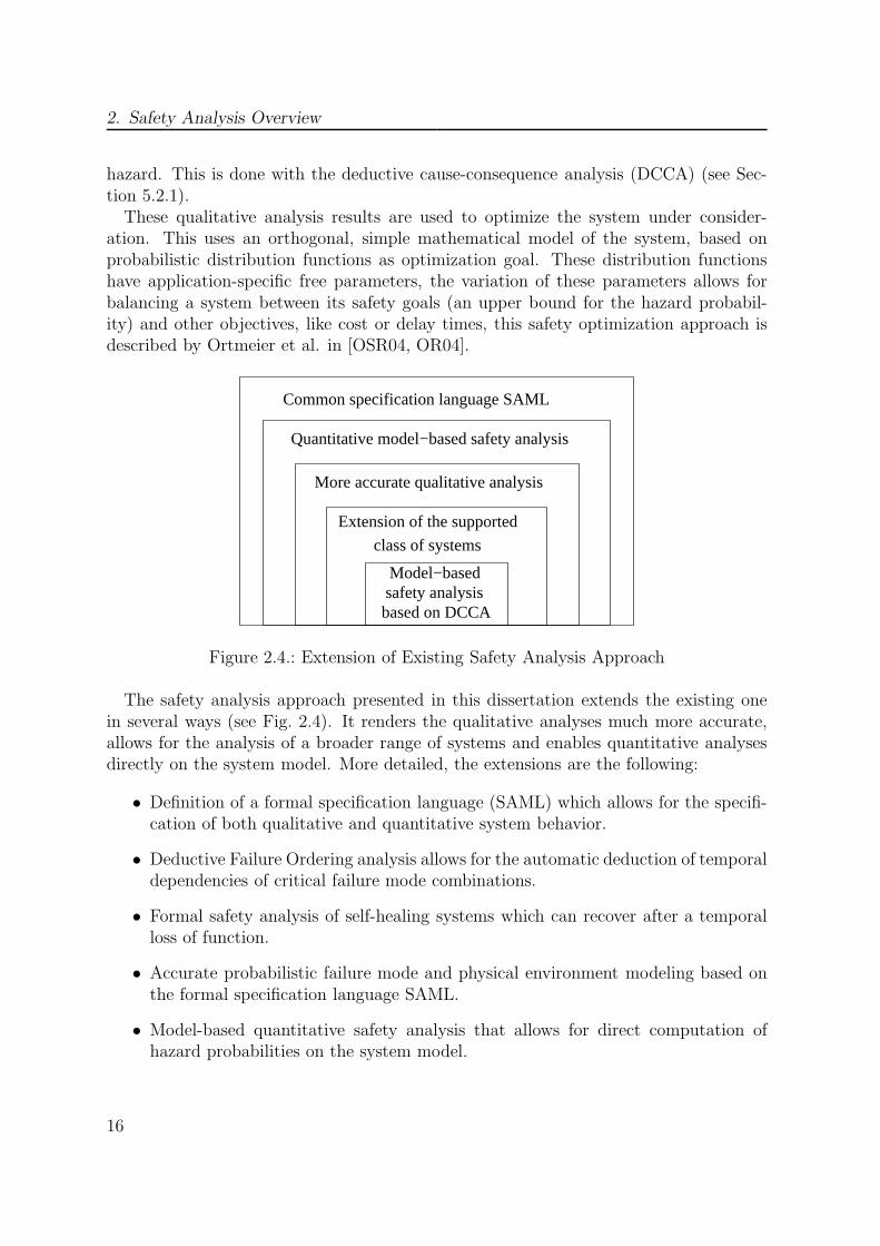
Figure 2.4.: Extension of Existing Safety Analysis Approach
The safety analysis approach presented in this dissertation extends the existing onein several ways (see Fig. 2.4). It renders the qualitative analyses much more accurate,allows for the analysis of a broader range of systems and enables quantitative analysesdirectly on the system model. More detailed, the extensions are the following:
• Definition of a formal specification language (SAML) which allows for the specifi-cation of both qualitative and quantitative system behavior.
• Deductive Failure Ordering analysis allows for the automatic deduction of temporaldependencies of critical failure mode combinations.
• Formal safety analysis of self-healing systems which can recover after a temporalloss of function.
• Accurate probabilistic failure mode and physical environment modeling based onthe formal specification language SAML.
• Model-based quantitative safety analysis that allows for direct computation ofhazard probabilities on the system model.
16

2.5. Formal Model-Based Safety Analysis
• Concrete implementation of model transformations of SAML models into the spec-ification languages of different formal analysis tools.
Because of the implemented model transformations, the approach is tool-independentand therefore benefits from any increased efficiency of the already supported analysistools. In addition, the integration of new analysis tools, e.g. those developed in theAVACS project, is possible by implementing the corresponding model transformations.SAML is designed to be well suited for the actual model specification as it offers aconvenient textual representation of both qualitative and quantitative behavior of asystem. The increased accuracy of the computed hazard probabilities also make it anideal candidate in a completely model-based safety optimization approach as proposedfor the ProMoSA project [OG10], replacing the approximations via distribution functionspreviously developed by Ortmeier et al. for safety optimization [OSR04, OR04].
Summary
This chapter presented the definition of the basic concepts of safety, hazard and failuremode as used in this dissertation. It gave an overview of different existing approachesfor safety analysis, namely purely structured approaches, failure propagation based ap-proaches and failure-injection based approaches. It outlined the benefits of the approachproposed in this dissertation which greatly extends the existing qualitative safety anal-ysis approach based on DCCA and allows for much more precise quantitative analysesthan possible before.
17

3. Formal Basics
Make things as simple as possible, but not simpler.
(Albert Einstein)
This chapter introduces the formal foundations of the qualitative and quantitativeformal model-based safety analysis. At first the syntax of the Safety Analysis andModeling Language (SAML) is defined which serves as modeling framework. Its formalsemantics is based on Markov chain models from probability theory.Properties of SAML models are formulated as temporal logic proof obligations. The
semantics of different temporal logics are presented, qualitative properties are specifiedin computational tree logic (CTL) and linear time logic (LTL), quantitative propertiesin a probabilistic temporal logic (PCTL).The motivations for the design of SAML are explained in Section 3.1. Its syntax is
presented in Section 3.2 together with a small example model. Section 3.3 describesthe semantics of the underlying formal models by providing its formal definition andalso an illustration of the semantics of the introduced example. In Section 3.4 temporallogics for both qualitative and probabilistic assertions are introduced which are used inlater chapters to specify the various formal analyses. Section 3.5 introduces a convenientgraphical representation of SAML modules. Related work is discussed in Section 3.6.
19

3. Formal Basics
3.1. Motivation
A specification framework for the analysis of safety-critical systems has several strongrequirements. The most important aspects are the following:
1. Feasibility of formal analysis by using formal semantics
2. Efficient transformation of models into the specification frameworks of existingstate of the art formal analysis tools
3. Convenient system modeling directly in the framework
4. Expressibility of probabilistic and non-deterministic behavior
Having formal semantics and being able to transform the language into existing for-mal analysis tools are somehow antagonistic to the requirement that direct modeling isconvenient. On the one hand, if too many high level modeling artifacts are introduced,their expression as a formal model can get very complicated and lead to state explosionwhich makes formal analysis unfeasible for all but very simple models. On the otherhand, it is often very difficult to create models in a specification language that is veryclose to the analysis model of a tool, comparable to programming in assembly language.Therefore a compromise between convenient modeling and formal aspects is needed.
SAML allows for the specification via parallel finite state automata. These can easilybe visualized which is very useful to visualize models and to analyze analysis results.A formal semantics is defined by specifying a parallel composition of the finite stateautomata and the semantics of the resulting product automaton. Finite state automataare also the basis for the analysis model for most state of the art analysis tools. Thisallows for the efficient transformation of SAML models into models suitable for thesetools.For accurate quantitative model-based safety analysis, a possibility to model proba-
bilistic behavior as well as non-deterministic behavior is necessary. Not only the isolatedcorrectness of a modeled system itself is of interest, but its behavior in a real environ-ment. This environment includes failing components as well as non-exact or unforeseenphysical behavior. A lot of this type of behavior can be described in concepts of proba-bilities, e.g. as failure rates or via probabilistic distributions. On the other hand, if thecorrect probabilities are not known or a behavior is inherently not probabilistic, thennon-deterministic modeling is often more adequate. Therefore both non-deterministicand probabilistic modeling is possible in SAML and an explicit timing model is specifiedfor accurate environment modeling.Its design allows SAML to be both a modeling language in which safety-critical sys-
tems and their environment can be expressed and analyzed, as well as a potential in-termediate language. SAML is tool-independent and supports the transformation ofmodels into input specifications of different formal analysis tools. Therefore any lan-guage that can be transformed into SAML benefits from this, as its models can also
20
3.2. Syntax of the Formal Models
be analyzed with all tools supported in the SAML framework. SAML has been firstpresented in [GO10a]. Transformations for widely used verification tools is explained inChapter 6. In the outlook in Chapter 8, some further ideas for language extensions builton top of SAML will be discussed.
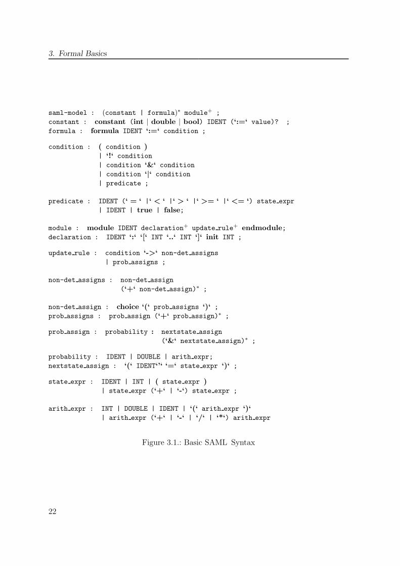
3.2. Syntax of the Formal Models
The most important aspects of the grammar for SAML models is shown in ExtendedBackus Naur Form (EBNF) in Fig. 3.1. Keywords and symbols are presented in boldfont, symbols are enclosed between ‘ for better visibility. The keywords are: constant,formula, int, double, bool, true, false, module, endmodule, init and choice.IDENT is a general lexer rule for identifiers, DOUBLE and INT are lexer ruler fordouble, respectively integral numbers.Lexer rules start in uppercase, parser rules in lowercase. The actual implementation of
SAML is realized as a grammar specification for the ANTLR parser generator developedby Parr [Par07] with Java as target language.
SAML Language Concepts
The syntax of SAML is basically an extended subset of the input language of thePRISM model-checker developed by Kwiatkowska et al. [KNP02b]. The most promi-nent differences are the omission of explicit synchronization labels and the explicitnessof non-deterministic choices with the choice keyword. The explicit indication of non-determinism has the advantage that it is less likely to be missed when reading such amodel specification. It also prevents some modeling which is not in accordance with theproposed modeling approach for safety critical systems presented in the next chapter.
SAML Model A SAML model consists of various definitions of constants and formulasand of one or more SAML modules. These modules represent finite state automata thatare executed in a synchronously parallel manner.
Constants A constant has an associated name, the identifier, a type and an optionalvalue. The values can either specified directly or as an arithmetic expression. The typeof a constant is either double, int or bool.
Value A value is either an integral value, a Boolean value or a floating point value.Floating point values can be expressed in scientific notation.
Formulas A formula is comprised of its name and a Boolean condition. It is generallyused to specify an abbreviation of a more complex Boolean expression.
21
3. Formal Basics
saml-model : (constant | formula)∗ module+ ;
constant : constant (int | double | bool) IDENT (‘:=‘ value)? ;
formula : formula IDENT ‘:=‘ condition ;
condition : ( condition )| ‘!‘ condition
| condition ‘&‘ condition
| condition ‘|‘ condition
| predicate ;
predicate : IDENT (‘ = ‘ |‘ < ‘ |‘ > ‘ |‘ >= ‘ |‘ <= ‘) state expr
| IDENT | true | false;
module : module IDENT declaration+ update rule+ endmodule;declaration : IDENT ‘:‘ ‘[‘ INT ‘..‘ INT ‘]‘ init INT ;
update rule : condition ‘->‘ non-det assigns
| prob assigns ;
non-det assigns : non-det assign
(‘+‘ non-det assign)∗ ;
non-det assign : choice ‘(‘ prob assigns ‘)‘ ;
prob assigns : prob assign (‘+‘ prob assign)∗ ;
prob assign : probability : nextstate assign
(‘&‘ nextstate assign)∗ ;
probability : IDENT | DOUBLE | arith expr;
nextstate assign : ‘(‘ IDENT‘’‘ ‘=‘ state expr ‘)‘ ;
state expr : IDENT | INT | ( state expr )| state expr (‘+‘ | ‘-‘) state expr ;
arith expr : INT | DOUBLE | IDENT | ‘(‘ arith expr ‘)‘| arith expr (‘+‘ | ‘-‘ | ‘/‘ | ‘*‘) arith expr
Figure 3.1.: Basic SAML Syntax
22
3.2. Syntax of the Formal Models
Condition A condition is a Boolean expression in propositional logic. It is comprisedof negation, conjunction or disjunction of conditions or predicates.
Predicate A predicate is a Boolean truth value or a predicate of expressions over thestate variables or a reference to a formula identifier.
Modules Each module declaration has a name and is contained between the keywordsmodule and endmodule. Within a module at least one state variable is declared and atleast one update rule is specified.
Declaration State variables have an associated identifier as name, are of integral type,have a single initial value and represent a range with lower and upper bound.
Update Rules An update rule is comprised of a Boolean activation condition and hasat least one non-deterministic choice for assignments or a single probabilistic assignment.Each non-deterministic choice is characterized by the choice keyword. If several suchnon-deterministic choices are specified, they are written as a sum.
Non-Deterministic Assignment Each non-deterministic assignment consists of one ormore probabilistic assignments.
Probabilistic Assignment Each single probabilistic assignment starts with its proba-bility. This probability can be given directly as value of type double, as a floating pointconstant or as an arithmetic expression. The probability is then followed by parallelassignments of new values to state variables.
Parallel Assignments Each assignment of a new value refers to the name of the statevariable and a state expression. The assignments are separated from each other with &.For a state variable v, the name for the next value is written as v’. A state expressiondefines this new value v’ which can be either an integral value, the name of a constantor an arithmetic expression. It is required, that in each parallel assignment all variablesof the respective module get a new value assigned.
State Expressions State expressions are generally an expression over the value of thestates. As states are of integral value, state expressions allow to specify the sum ordifference of the value of states. They can also consist directly of an identifier referringto a state variable, an integral constant or directly an integral value.
Arithmetic Expressions An arithmetic expression can be the sum, difference, quotientor product of integral values or doubles, specified as constants or directly via values.The interpretation of sum, difference, quotient and product is the standard one.
23
3. Formal Basics
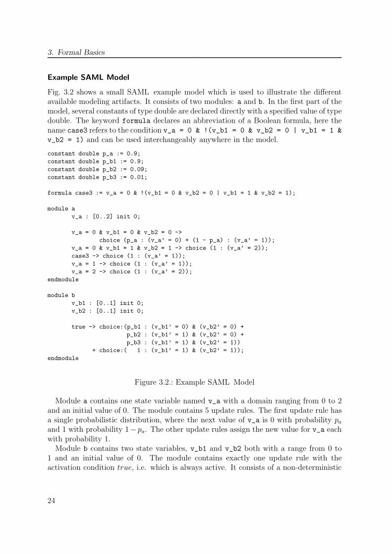
Example SAML Model
Fig. 3.2 shows a small SAML example model which is used to illustrate the differentavailable modeling artifacts. It consists of two modules: a and b. In the first part of themodel, several constants of type double are declared directly with a specified value of typedouble. The keyword formula declares an abbreviation of a Boolean formula, here thename case3 refers to the condition v_a = 0 & !(v_b1 = 0 & v_b2 = 0 | v_b1 = 1 &
v_b2 = 1) and can be used interchangeably anywhere in the model.
constant double p_a := 0.9;
constant double p_b1 := 0.9;
constant double p_b2 := 0.09;
constant double p_b3 := 0.01;
formula case3 := v_a = 0 & !(v_b1 = 0 & v_b2 = 0 | v_b1 = 1 & v_b2 = 1);
module a
v_a : [0..2] init 0;
v_a = 0 & v_b1 = 0 & v_b2 = 0 ->
choice (p_a : (v_a’ = 0) + (1 - p_a) : (v_a’ = 1));
v_a = 0 & v_b1 = 1 & v_b2 = 1 -> choice (1 : (v_a’ = 2));
case3 -> choice (1 : (v_a’ = 1));
v_a = 1 -> choice (1 : (v_a’ = 1));
v_a = 2 -> choice (1 : (v_a’ = 2));
endmodule
module b
v_b1 : [0..1] init 0;
v_b2 : [0..1] init 0;
true -> choice:(p_b1 : (v_b1’ = 0) & (v_b2’ = 0) +
p_b2 : (v_b1’ = 1) & (v_b2’ = 0) +
p_b3 : (v_b1’ = 1) & (v_b2’ = 1))
+ choice:( 1 : (v_b1’ = 1) & (v_b2’ = 1));
endmodule
Figure 3.2.: Example SAML Model
Module a contains one state variable named v_a with a domain ranging from 0 to 2and an initial value of 0. The module contains 5 update rules. The first update rule hasa single probabilistic distribution, where the next value of v_a is 0 with probability paand 1 with probability 1− pa. The other update rules assign the new value for v_a eachwith probability 1.Module b contains two state variables, v_b1 and v_b2 both with a range from 0 to
1 and an initial value of 0. The module contains exactly one update rule with theactivation condition true, i.e. which is always active. It consists of a non-deterministic
24
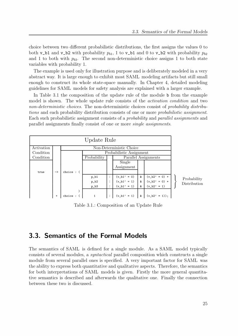
3.3. Semantics of the Formal Models
choice between two different probabilistic distributions, the first assigns the values 0 toboth v_b1 and v_b2 with probability pb1, 1 to v_b1 and 0 to v_b2 with probability pb2and 1 to both with pb3. The second non-deterministic choice assigns 1 to both statevariables with probability 1.
The example is used only for illustration purpose and is deliberately modeled in a veryabstract way. It is large enough to exhibit most SAML modeling artifacts but still smallenough to construct its whole state-space manually. In Chapter 4, detailed modelingguidelines for SAML models for safety analysis are explained with a larger example.
In Table 3.1 the composition of the update rule of the module b from the examplemodel is shown. The whole update rule consists of the activation condition and twonon-deterministic choices. The non-deterministic choices consist of probability distribu-tions and each probability distribution consists of one or more probabilistic assignment.Each such probabilistic assignment consists of a probability and parallel assignments andparallel assignments finally consist of one or more single assignments.
Update Rule
Activation Non-Deterministic ChoiceCondition Probabilistic AssignmentCondition Probability Parallel Assignments
SingleAssignment
true -> choice : (
p_b1 : (v_b1’ = 0) & (v_b2’ = 0) +
Probabilityp_b2 : (v_b1’ = 1) & (v_b2’ = 0) +
Distributionp_b3 : (v_b1’ = 1) & (v_b2’ = 1)
)
+ choice : ( 1 : (v_b1’ = 1) & (v_b2’ = 1));
Table 3.1.: Composition of an Update Rule
3.3. Semantics of the Formal Models
The semantics of SAML is defined for a single module. As a SAML model typicallyconsists of several modules, a syntactical parallel composition which constructs a singlemodule from several parallel ones is specified. A very important factor for SAML wasthe ability to express both quantitative and qualitative aspects. Therefore, the semanticsfor both interpretations of SAML models is given. Firstly the more general quantita-tive semantics is described and afterwards the qualitative one. Finally the connectionbetween these two is discussed.
25
3. Formal Basics
3.3.1. Parallel Composition
The parallel composition transforms a SAML model with several modules into an equiv-alent model with a single module. The semantics of a SAML model is defined in Sec-tion 3.3.2 based on this single module. For the parallel composition of two modules, theparallel composition operator || is used analogously to the synchronous parallel compo-sition described by Norman et al. in [NPK10].Every update rule of a SAML model contains parallel assignments of new values to
the state variables. For a state variable v, v′ denotes its value for the next time step.The assigned value is an expression over the other state variables, constants and integers.The common interpretation of addition and subtraction for + and − is used. Parallelassignments to several state variables are denoted by the operator & in the form:
v′1 = exprV ar1 & · · ·&v′n = exprV ar
n
Each possible variable assignment has an corresponding probability p and is of the form:
p :(
v′1 = exprV ar1 & · · ·&v′n = exprV ar
n
)
Several of these parallel variable assignments form a discrete probability distribution,which requires that
∑
i pi = 1:
p1 : (v′1 = expr11&v
′2 = expr12& · · ·&v′m = expr1m)+
· · ·
pn : (v′1 = exprn1&v′2 = exprn2& · · · v′m = exprnm))
Each update rule of a SAML model is comprised of one or more non-deterministicchoices, where each such choice corresponds to exactly one of these discrete probabilitydistributions of transitions. Together with the Boolean activation condition φi, thegeneral form of an update rule is as follows:
φi → choicei1 : ( pi11 : (v′1 = expr111&v
′2 = expr112& · · ·&v′m = expr11m) + · · ·
pi1n : (v′1 = expr1n1&v′2 = expr1n2& · · · v′m = expr1nm))
...
+ choiceik : ( pik1 : (v′1 = exprk11&v
′2 = exprk12& · · ·&v′m = exprk1m) + · · ·
pikn : (v′1 = exprkn1&v′2 = exprkn2& · · · v′m = exprknm)) (3.1)
For simplicity it is assumed that all the requirements for a proper specification arefulfilled. This means that the probabilities specify correct probability distributions and
26
3.3. Semantics of the Formal Models
that the variables are uniquely named, i.e. there are no modules that contain a variablewith the same name.This notation is chosen to simplify the usage of update rules in the parallel composition
definition. The single update rule of the module b (see table 3.1) of the example abovewould be written in the following way:
true→ choice : ( pb1 : (v′b1 = 0&v′b2 = 0) +
pb2 : (v′b1 = 1&v′b2 = 0) +
pb3 : (v′b1 = 1&v′b2 = 1))
+ choice : ( 1 : (v′b1 = 1&v′b2 = 1))
Using this notation, update rules can be written using the mathematical notation forsums and the parallel composition of two SAML modules with the operator || can bedefined as in Def. 1 which is adapted from Kwiatkowska et al. [NPK10]. For two modulesMi and Mj , each probability distribution of each of the non-deterministic choices of thefirst module (Eq. (3.2)) is combined with each probability distribution of each of thenon-deterministic choices of the second module (Eq. (3.3)). The result is an updaterule with an activation condition which is the conjunction of the activation conditionsof the original update rules. Each of these choices is comprised of a new probabilitydistribution and parallel assignments of the state variables.
Definition 1. Parallel Composition of SAML ModulesFor M = Mi||Mj set stateV ars(M) := stateV ars(Mi) ∪ stateV ars(Mj) and create
for each update rule
φi →c∑
k=1
choiceik
(
dk∑
l=1
pikl : uikl
)
(3.2)
of Mi and
φj →e∑
m=1
choicejm
(
fm∑
n=1
pjmn : ujmn
)
(3.3)
of Mj a product update rule for M of the form
φi ∧ φj →c∑
k=1
e∑
m=1
choice
(
dk∑
l=1
fm∑
n=1
(
pikl · pjmn : uikl&u
jmn
)
)
This parallel composition is well-defined and unique. The variable ordering in theparallel assignments does not change the semantics of the result. Reordering of variablesin the parallel assignments or in the definition of state variables creates an isomorphicstate space. Therefore the semantics of the underlying Markov chain model is invariant
27

3. Formal Basics
under ordering of state variable definitions or parallel assignments1. If a SAML modelhas more than two modules, the parallel composition is conducted iteratively. A completeSAML model is defined as the parallel composition of its modules (Def. 2).
Definition 2. Complete ModelFor a SAML model which consists of the single modules M1, . . .Mn, the complete
model M is defined as M :=M1|| · · · ||Mn.
The complete model generated from the parallel composition a_b := a||b of the twomodules of the example of Fig. 3.2 is shown in Fig. 3.3. The complete model is comprisedof 5 updates rules, resulting from 5 update rules of module a and 1 update rule frommodule b. Each update rule of the complete model consists of two choices, resultingfrom the 2 choices of module b and 1 choice of module a. In the first update rule ofthe product module a_b, the first choice has 6 possible transitions, resulting from theproduct of 2 possibilities in the first choice of module a and 3 possibilities in the firstchoice of module b. The second update rule of a_b has 2 possible transitions, resultingfrom the 2 possibilities of module a and only 1 possibility of module b. The rest of theupdate rules are constructed analogously.From the length and complexity of the complete model resulting from the parallel
composition of the rather simple modules of the originating SAML model, it becomesclear that direct specification of the complete module is not practical. Therefore ingeneral multiple parallel modules are specified in SAML and the construction of thesingle module is left to the specific analysis tool.The informal semantics of a SAML model is as follows: All the modules of the original
model are executed synchronously in parallel. At each time step, all activation conditionsof each module are evaluated. The models are constructed in such a way that there isalways exactly one active update rule per module per time-step. In every module, oneprobability distribution of the active update rule is chosen non-deterministically. Thisprobability distribution is a set of assignments of new values for all the state variablesof the module. One of these assignments is then chosen probabilistically and the statevariables get new values assigned in parallel. The parallel composition retains thisbehavior, but combines all the modules into one single module in which the update rulesare the enumeration of all possible combinations of updates rules of the original model.
3.3.2. Quantitative Formal Models
The basis for the formal semantics of SAML is a variant of Markov chains which canexpress both probabilistic and non-deterministic behavior. Markov chain models areoften used for modeling probabilistic behavior. Different variants exist which are appro-priate for different modeling applications. Markov models basically describe a systemas discrete states with probabilistic transitions between these states.
1The internal representation of the state space often uses variable reordering to achieve a more compactrepresentation.
28

3.3. Semantics of the Formal Models
module a_b
v_a : [0..2] init 0;
v_b1 : [0..1] init 0;
v_b2 : [0..1] init 0;
true & v_a = 0 & v_b1 = 0 & v_b2 = 0 ->
choice (p_b1 * p_a : (v_a’ = 0) & (v_b1’ = 0) & (v_b2’ = 0)
+ p_b1 * (1 - p_a) : (v_a’ = 1) & (v_b1’ = 0) & (v_b2’ = 0)
+ p_b2 * p_a : (v_a’ = 0) & (v_b1’ = 1) & (v_b2’ = 0)
+ p_b2 * (1 - p_a) : (v_a’ = 1) & (v_b1’ = 1) & (v_b2’ = 0)
+ p_b3 * p_a : (v_a’ = 0) & (v_b1’ = 1) & (v_b2’ = 1)
+ p_b3 * (1 - p_a) : (v_a’ = 1) & (v_b1’ = 1) & (v_b2’ = 1))
+ choice (1 * p_a : (v_a’ = 0) & (v_b1’ = 1) & (v_b2’ = 1)
+ 1 * (1 - p_a) : (v_a’ = 1) & (v_b1’ = 1) & (v_b2’ = 1));
true & v_a = 0 & v_b1 = 1 & v_b2 = 1 ->
choice (p_b1 * 1 : (v_a’ = 2) & (v_b1’ = 0) & (v_b2’ = 0)
+ p_b2 * 1 : (v_a’ = 2) & (v_b1’ = 1) & (v_b2’ = 0)
+ p_b3 * 1 : (v_a’ = 2) & (v_b1’ = 1) & (v_b2’ = 1))
+ choice (1 * 1 : (v_a’ = 2) & (v_b1’ = 1) & (v_vb2’ = 1));
true & v_a = 0 & !(v_b1 = 0 & v_b2 = 0 | v_b1 = 1 & v_b2 = 1) ->
choice (p_b1 * 1 : (v_a’ = 1) & (v_b1’ = 0) & (v_b2’ = 0)
+ p_b2 * 1 : (v_a’ = 1) & (v_b1’ = 1) & (v_b2’ = 0)
+ p_b3 * 1 : (v_a’ = 1) & (v_b1’ = 1) & (v_b2’ = 1))
+ choice (1 * 1 : (v_a’ = 2) & (v_b1’ = 1) & (v_vb2’ = 1));
true & v_a = 1 ->
choice (p_b1 * 1 : (v_a’ = 1) & (v_b1’ = 0) & (v_b2’ = 0)
+ p_b2 * 1 : (v_a’ = 1) & (v_b1’ = 1) & (v_b2’ = 0)
+ p_b3 * 1 : (v_a’ = 1) & (v_b1’ = 1) & (v_b2’ = 1))
+ choice (1 * 1 : (v_a’ = 1) & (v_b1’ = 1) & (v_vb2’ = 1));
true & v_a = 2 ->
choice (p_b1 * 1 : (v_a’ = 2) & (v_b1’ = 0) & (v_b2’ = 0)
+ p_b2 * 1 : (v_a’ = 2) & (v_b1’ = 1) & (v_b2’ = 0)
+ p_b3 * 1 : (v_a’ = 2) & (v_b1’ = 1) & (v_b2’ = 1))
+ choice (1 * 1 : (v_a’ = 2) & (v_b1’ = 1) & (v_vb2’ = 1));
endmodule
Figure 3.3.: Parallel Composition of the SAML Model of Fig. 3.2
29
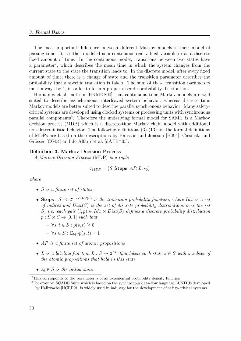
3. Formal Basics
The most important difference between different Markov models is their model ofpassing time. It is either modeled as a continuous real-valued variable or as a discretefixed amount of time. In the continuous model, transitions between two states havea parameter2, which describes the mean time in which the system changes from thecurrent state to the state the transition leads to. In the discrete model, after every fixedamount of time, there is a change of state and the transition parameter describes theprobability that a specific transition is taken. The sum of these transition parametersmust always be 1, in order to form a proper discrete probability distribution.Hermanns et al. note in [HKMKS00] that continuous time Markov models are well
suited to describe asynchronous, interleaved system behavior, whereas discrete timeMarkov models are better suited to describe parallel synchronous behavior. Many safety-critical systems are developed using clocked systems or processing units with synchronousparallel components3. Therefore the underlying formal model for SAML is a Markovdecision process (MDP) which is a discrete-time Markov chain model with additionalnon-deterministic behavior. The following definitions (3)-(13) for the formal definitionsof MDPs are based on the descriptions by Hansson and Jonsson [HJ94], Ciesinski andGrosser [CG04] and de Alfaro et al. [dAFH+05].
Definition 3. Markov Decision ProcessA Markov Decision Process (MDP) is a tuple
τMDP = (S,Steps, AP, L, s0)
where
• S is a finite set of states
• Steps : S → 2Idx×Dist(S) is the transition probability function, where Idx is a setof indices and Dist(S) is the set of discrete probability distributions over the setS, i.e. each pair (i, p) ∈ Idx × Dist(S) defines a discrete probability distributionp : S × S → [0, 1] such that
– ∀s, t ∈ S : p(s, t) ≥ 0
– ∀s ∈ S : Σt∈Sp(s, t) = 1
• AP is a finite set of atomic propositions
• L is a labeling function L : S → 2AP that labels each state s ∈ S with a subset ofthe atomic propositions that hold in this state
• s0 ∈ S is the initial state
2This corresponds to the parameter λ of an exponential probability density function.3For example SCADE Suite which is based on the synchronous data-flow language LUSTRE developedby Halbwachs [HCRP91] is widely used in industry for the development of safety-critical systems.
30

3.3. Semantics of the Formal Models
A MDP as in Def. 3 represents a labeled transition system with a finite set of states.Each state s ∈ S corresponds to a valuation of all state variables of a single SAMLmodule, in general the complete model of parallel SAML modules . The initial valuationof the state variables in the model correspond to the initial state so of the MDP. Eachstate s is labeled with the set of atomic propositions (AP ) that hold in s by the labelingfunction L. By the definition of L, all ψ ∈ AP : ψ 6∈ L(s) do not hold in s. InSAML, these atomic propositions correspond to the set of conditions, i.e. are Booleanexpressions over the values of the state variables of the model.The update rules of the SAML model describe the possible transitions of the MDP.
Each activation condition φ describes a subset S ′ ⊆ S of all states such that for eachstate s ∈ S ′, its label L(s) implies φ. For each state s, Steps(s) maps s to a set ofpairs of indices and discrete probability distributions. These describe the probability ofreaching a successor state s′ from s, where s′ corresponds to a new valuation of the statevariables of the model. The index specifies which probability distribution is chosen. Theprobability distribution specifies the probability to reach successor states.The state space of the parallel composition of the example in Fig. 3.2 is shown in
Fig. 3.4. Each node corresponds to a state of the MDP. Each state represents a valuationof the state variables, written inside the nodes as a vector of the form (v_a,v_b1,v_b2).There is an edge from state s to s′ if there exists an index and probability distributionpair (i, p) in Steps(s), such that p(s, s′) > 0, i.e. the state s′ is reachable from state swith non-zero probability.The edges represent these probability distributions. They are labeled in the form
j : pj , where j is the index of the possible probability distributions in Steps(s) and pjis the probability to reach the state s′ from s if the probability distribution p is chosen,i.e. pj = p(s, s′).The paths of the MDP are all infinite sequences of states (starting from the initial
state (0,0,0)) and probabilities such that for each successor state s′ of a state s thereexists a directed edge from s to s′ in the graph representation of the state space.This describes the semantics of a SAML module as a MDP. In order to be interpretable
in such a way, a SAML module must fulfill the following constraints on the activationconditions and probabilities of the update rules:
1.∑
i pi = 1 for each probabilistic assignment and pi > 0 for each probability
2.∨
i φi ≡ true for all activation conditions φi
3. ∀i 6= j : φi ∧ φj ≡ false for each pair of activation conditions
The first constraint states that every probabilistic assignment must define a properdiscrete probability distribution, by demanding that the probabilities to reach a newstate sum to 1. The second constraint specifies that there is always an activation con-dition that holds. This means, in every state s there exists at least one element inSteps(s). These two constraints assure that there is always a successor state that can
31
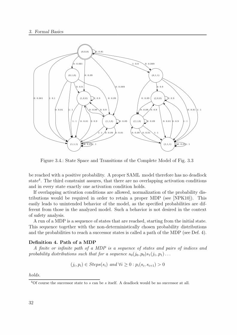
3. Formal Basics
(0,0,0) 0 : 0 .81
(0,1,0)
0 : 0 .081
(0,1,1)
0 : 0 .0091: 0.9
(1,0,0)
0 : 0 .09
(1,1,0)
0 : 0 .009
(1,1,1)
0 : 0 .001 1: 0.1
0: 0.9
0: 0 .09
0: 0 .01 1: 1
(2,0,0)
0: 0 .9
(2,1,0)
0 : 0 .09
(2,1,1)
0 : 0 .01 1: 1
0: 0 .9
0: 0 .09
0: 0 .011: 1
0: 0 .9
0: 0 .09
0: 0 .011: 1
0: 0 .9
0: 0 .09
0: 0 .011: 1
0: 0 .9
0: 0 .09
0: 0 .01 1: 1
0: 0 .9
0: 0 .09
0: 0 .01 1: 1
0: 0 .9
0: 0 .09
0: 0 .011: 1
Figure 3.4.: State Space and Transitions of the Complete Model of Fig. 3.3
be reached with a positive probability. A proper SAML model therefore has no deadlockstate4. The third constraint assures, that there are no overlapping activation conditionsand in every state exactly one activation condition holds.If overlapping activation conditions are allowed, normalization of the probability dis-
tributions would be required in order to retain a proper MDP (see [NPK10]). Thiseasily leads to unintended behavior of the model, as the specified probabilities are dif-ferent from those in the analyzed model. Such a behavior is not desired in the contextof safety analysis.A run of a MDP is a sequence of states that are reached, starting from the initial state.
This sequence together with the non-deterministically chosen probability distributionsand the probabilities to reach a successor states is called a path of the MDP (see Def. 4).
Definition 4. Path of a MDPA finite or infinite path of a MDP is a sequence of states and pairs of indices and
probability distributions such that for a sequence s0(j0, p0)s1(j1, p1) . . .
(ji, pi) ∈ Steps(si) and ∀i ≥ 0 : pi(si, si+1) > 0
holds.
4Of course the successor state to s can be s itself. A deadlock would be no successor at all.
32

3.3. Semantics of the Formal Models
When all states of a path are labeled with their labeling function, the resulting se-quence is called a trace of the MDP (see. Def. 5). Properties of the MDP are most oftenformulated based on the set of possible traces.
Definition 5. Trace of a MDPA trace σ of a path ω = s0(j0, p0)s1(j1, p1) . . . of a MDP Model τMDP is the word over
the alphabet 2AP , generated from
σ(s0(j0, p0)s1(j1, p1) . . .) = L(s0)L(s1) · · ·
In a path of a MDP, every state s is followed by a pair (j, p). This describes an indexj and a probability p. Here j is the index of the non-deterministically chosen probabilitydistribution P of Steps(s). This distribution describes a probability p = P (s, s′) as theprobability to make the step from s to s′ in the MDP. By definition p > 0 holds if s′
is a successor of s on a path of the MDP. A valid sequence of indices and probabilitydistributions is described by an adversary (see Def. 6).
Definition 6. Adversary / SchedulerAn adversary A of an MDP τMDP is a function that maps all finite paths ω =
s0(j0, p0)s1 . . . sn to one element of Steps(sn).
An adversary describes an infinite sequence of non-deterministic choices of probabil-ity distributions. A specific adversary resolves the non-determinism by defining whichprobability distribution is chosen from Steps(sn) for every finite path of the MDP.In general there are infinitely many adversaries possible in a MDP. Of most interest
are the “worst-case” and “best-case” adversaries, which always make the “worst” or“best” decision. This will be discussed in more detail in Section 3.4. Here, the adver-saries are used to eliminate non-determinism from the model (an adversary consists ofconcrete choices) by projecting the non-deterministic choices onto one specific determin-istic model. In order to get a probability measure for MDP using adversaries, a formalmodel of such deterministic probabilistic behavior is needed (see. Def. 7).
Definition 7. Discrete Time Markov ChainA discrete time Markov chain (DTMC) is a tuple
τDTMC = (S, p, AP, L, s0)
where
• S is a finite or infinite, non-empty set of states
• p : S × S → [0, 1] is a function such that ∀s ∈ S:
– ∀s, t ∈ S : p(s, t) ≥ 0
– Σt∈Sp(s, t) = 1
33

3. Formal Basics
• AP is a finite set of atomic propositions
• L is a labeling function L : S → 2AP that labels each state s ∈ S with a subset ofthe atomic propositions that hold in this state
• s0 ∈ S is the initial state
A DTMC is a special case of a MDP that has a constant Steps function, where onlya single global probability distribution exists to choose from. Paths (Def. 8) and traces(Def. 9) are defined analogously to paths and traces of a MDP. The difference here isthat a path is comprised of a sequence of only states.
Definition 8. Path of a DTMCA path π of a DTMC model τDTMC is a finite or infinite sequence of states si ∈ S of
the form π = s0, s1, . . . and p(si, si+1) > 0.
Definition 9. Trace of a DTMCA trace σ of a path π = s0, s1, . . . of a DTMC Model τ is the word over the alphabet
2AP , generated fromσ(π) = L(s0)L(si) · · ·
Every finite path π of a DTMC has an associated set of infinite paths called the basiccylinder (Def. 10). Each infinite path in the basic cylinder has π as a prefix, i.e. theelements of the basic cylinder of π are all infinite postfixes of π.
Definition 10. Basic Cylinder of a DTMCFor any finite path π of a DTMC, the set Pathinfin(π) of infinite postfixes of π, the
basic cylinder is defined as
∆(π) = {ρ ∈ Pathinfin(π)|π is prefix of ρ}
This basic cylinder is used to define the probability space for a DTMC as in Def. 11. Itdefines a probability measure for the infinite continuations of a finite path of a DTMC.
Definition 11. Probability Space of DTMC ModelFor τDTMC = (S, p, AP, L, so) and s ∈ S, the probability space Υdtmc is defined as:
Υdtmc = (∆(s),∆s, probs)
such that
• ∆s is the σ-algebra generated by the empty set and the basic cylinders over S thatare contained in ∆(s).
• probs is the uniquely induced probability measure which satisfies the following:probs(∆(s0)) = 1 and for all basic cylinders ∆(s0, s1, . . . , sn) over S:
probs(∆(s0, s1, . . . , sn)) = p(s0, s1) · p(s1, s2) · . . . · p(sn−1, sn)
34

3.3. Semantics of the Formal Models
The probability measure is defined over the basic cylinders of finite paths. The pathstarting in s0 of length one, therefore has probability 1. For every finite path, theprobability of its basic cylinder is defined as the product of the probabilities to reachthe respective successor states on the path in the sequence they appear on it.This definition is sound, as from the definition of a DTMC it is known that from every
reachable state there is always a successor state. This means that from every reachablestate s there exists a continuation with probability 1 and no deadlock is possible. So fora finite path ending in state sn, the basic cylinder ∆(sn) is the set of all possible infinitecontinuations. Therefore the probability that a successor of sn exists on any of thosecontinuations is 1.
Definition 12. Probability Measure for Paths of an AdversaryFor each possible adversary A, a probability measure PrAs can be defined by considering
a variant of DTMC with infinitely many states τDTMC∞ = (PathAfin(s), T, P rAs , AP, L, s)
where
• the set of states PathAfin(s) are the finite paths starting in state s
• initial state s, the path starting in s with length 0
• PrAs (ω, ω′) = p(sn, s) if ω = s0(a0, p0)s1 . . . sn, ω
′ = ω(a, p)s and A(ω) = (a, p)
• PrAs (ω, ω′) = 0 otherwise
This probability measure for paths of an adversary is used to specify the probabilityspace of a MDP. Every adversary corresponds to an infinite sequence of non-deterministicchoices which projects a MDP to an infinite state DTMC. The states of this DTMCrepresent the finite paths starting in the state s. As there is an infinite number of finitepaths in the MDP, there are infinitely many states in the DTMC. If sn is the last state ofsuch a finite path, then the probability to reach a state s′ from sn is defined as P (sn, s
′)where P is the probability distribution chosen by the adversary at step n.
Definition 13. Probability Space of a MDPFor τMDP = (S,Steps, AP, L, s0), an adversary A and s ∈ S, the probability space
ΥAmdp is defined as:
ΥAmdp = (PathAinfin(s),Σ
As , P r
As )
such that
• ΣAMDP is the σ-algebra generated by the empty set and the infinite paths of the
associated (countable) infinite state DTMC τDTMC∞ = (PathAfin(s), P rAs , AP, L, s)
in Def. (12)
• PrAs is the uniquely induced probability measure as defined in Def. (12) such that
35

3. Formal Basics
– PrAs (PathAinfin(s)) = 1
– for a finite path ω = s0(j0, p0) · · · sn(jn, pn)sn+1 :
PrAs (PathAinfin(ω)) =
n−1∏
i=0
A(ω)(si+1)
So to compute the probability of the paths of a MDP, at first all non-deterministicchoices are resolved. This is done by choosing a specific adversary. This results inan infinite-state DTMC for which a probability measure can be defined as shown inDef. 11. As there are infinitely many possible adversaries, it is not possible to computethe probability for all. Realistically only two choices for adversaries are of interest, the“worst-case” and the “best-case” adversary5. A more detailed explanation about this isgiven in Section 3.4.
3.3.3. Qualitative Formal Model
For some analyses, probabilistic information is not relevant or desired. Reasons for thisare that the analysis itself does not make use of the probabilistic information or that thecomputation of the associated probabilities does not provide an advantage. An analysiswithout probabilistic information is called qualitative. An example for such a qualitativeanalysis would be the question: “Is a state s reachable from the initial state of a SAMLmodel?”. This is the same as computing the probability to reach the state s from theinitial state and using only the information that the probability is non-zero6.One prominent advantage of qualitative in contrast to quantitative analyses is that
they are easier and therefore less costly to compute. The reason is mainly that noarithmetic operations must be conducted and the state space can be represented in amore compact way. Therefore it is reasonable not to use quantitative analyses if anequivalent qualitative analysis method exists. This is supported in SAML by exploitingthe fact that every MDP has an associated Kripke structure which forms the basis forqualitative analyses. The following definitions (14)-(16) are adapted from Clarke etal. [CGP00] (pp. 14-15).
Definition 14. Kripke StructureA Kripke structure over a set AP of atomic propositions is a tuple
τKripke = (S, S0, T, L, AP )
with
5What the worst and best case is depends of course on the type of probability that is computed. Forsafety analysis the worst case is a higher probability of the occurrence of a hazardous situation.
6There are cases where an infinite path exists but has probability 0, this will be discussed in Section 3.4.
36

3.3. Semantics of the Formal Models
• S a finite, non-empty set of states
• S0 ⊆ S a set of initial states
• T ⊆ S × S a total transition relation, i.e. for each state s ∈ S there is a states′ ∈ S such that (s, s′) ∈ T holds
• L : S → 2AP is a mapping that labels each state s ∈ S with a subset of the atomicpropositions that hold in this state (all others are false)
The composition of a Kripke structure is similar to a MDP. It consists of a finite setof states, a labeling function and a set of atomic propositions. The difference here is theexistence of a transition relation instead of a Steps function. The transition relationeliminates the probability distributions and only non-deterministic behavior is retained.Due to this similarity, paths (Def. 15) and traces (Def. 16) of a Kripke structure can be
defined analogously as for MDPs. The only difference is the absence of the probabilitydistributions in the definition of a path.
Definition 15. Path of a Kripke StructureA path π of a Kripke structure τKripke is a finite or infinite sequence of states si ∈ S,
s0 ∈ So with (si, si+1) ∈ T of the form
π = s0, s1 . . .
Definition 16. Trace of a Kripke StructureA trace σ of path π = s0, s1 . . . of a Kripke structure τKripke is the word over the
alphabet 2AP , generated from
σ(π) = L(s0)L(s1) · · ·
Every SAML model has an embedded Kripke structure, which has the same statespace and transitions as the underlying MDP. This Kripke structure defines the quali-tative semantics of a SAML model. It is obtained by eliminating the probabilistic butkeeping the non-deterministic behavior of the SAML model.
Definition 17. Embedded Kripke StructureLet κ(τMDP ) be a mapping of the MDP
τMDP = (S,Steps, AP, L, s0)
to a tuple (S, {s0}, T, L, AP ) with
T := {(s, t)|s, t ∈ S ∧ ∃(j, p) ∈ Steps(s) : p(s, t) > 0}
then τKripke = (S, {s0}, T, L, AP ) is called the embedded Kripke structure of τMDP .
37
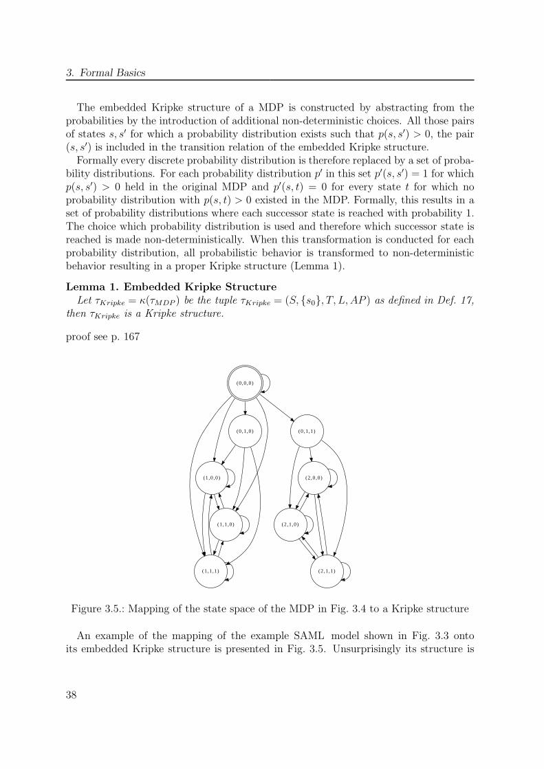
3. Formal Basics
The embedded Kripke structure of a MDP is constructed by abstracting from theprobabilities by the introduction of additional non-deterministic choices. All those pairsof states s, s′ for which a probability distribution exists such that p(s, s′) > 0, the pair(s, s′) is included in the transition relation of the embedded Kripke structure.Formally every discrete probability distribution is therefore replaced by a set of proba-
bility distributions. For each probability distribution p′ in this set p′(s, s′) = 1 for whichp(s, s′) > 0 held in the original MDP and p′(s, t) = 0 for every state t for which noprobability distribution with p(s, t) > 0 existed in the MDP. Formally, this results in aset of probability distributions where each successor state is reached with probability 1.The choice which probability distribution is used and therefore which successor state isreached is made non-deterministically. When this transformation is conducted for eachprobability distribution, all probabilistic behavior is transformed to non-deterministicbehavior resulting in a proper Kripke structure (Lemma 1).
Lemma 1. Embedded Kripke StructureLet τKripke = κ(τMDP ) be the tuple τKripke = (S, {s0}, T, L, AP ) as defined in Def. 17,
then τKripke is a Kripke structure.
proof see p. 167
(0,0,0)
(0,1,0) (0,1,1)
(1,0,0)
(1,1,0)
(1,1,1)
(2,0,0)
(2,1,0)
(2,1,1)
Figure 3.5.: Mapping of the state space of the MDP in Fig. 3.4 to a Kripke structure
An example of the mapping of the example SAML model shown in Fig. 3.3 ontoits embedded Kripke structure is presented in Fig. 3.5. Unsurprisingly its structure is
38
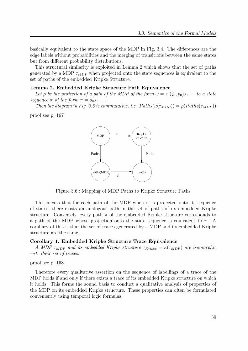
3.3. Semantics of the Formal Models
basically equivalent to the state space of the MDP in Fig. 3.4. The differences are theedge labels without probabilities and the merging of transitions between the same statesbut from different probability distributions.This structural similarity is exploited in Lemma 2 which shows that the set of paths
generated by a MDP τMDP when projected onto the state sequences is equivalent to theset of paths of the embedded Kripke Structure.
Lemma 2. Embedded Kripke Structure Path EquivalenceLet ρ be the projection of a path of the MDP of the form ω = s0(j0, p0)s1 . . . to a state
sequence π of the form π = s0s1 . . ..Then the diagram in Fig. 3.6 is commutative, i.e. Paths(κ(τMDP )) = ρ(Paths(τMDP )).
proof see p. 167
MDP
Paths(MDP)
Paths Paths
Kripkestructure
Paths
κ
ρ
Figure 3.6.: Mapping of MDP Paths to Kripke Structure Paths
This means that for each path of the MDP when it is projected onto its sequenceof states, there exists an analogous path in the set of paths of its embedded Kripkestructure. Conversely, every path π of the embedded Kripke structure corresponds toa path of the MDP whose projection onto the state sequence is equivalent to π. Acorollary of this is that the set of traces generated by a MDP and its embedded Kripkestructure are the same.
Corollary 1. Embedded Kripke Structure Trace EquivalenceA MDP τMDP and its embedded Kripke structure τKripke = κ(τMDP ) are isomorphic
wrt. their set of traces.
proof see p. 168
Therefore every qualitative assertion on the sequence of labellings of a trace of theMDP holds if and only if there exists a trace of its embedded Kripke structure on whichit holds. This forms the sound basis to conduct a qualitative analysis of properties ofthe MDP on its embedded Kripke structure. These properties can often be formulatedconveniently using temporal logic formulas.
39
3. Formal Basics
3.4. Temporal Logics
Temporal logic is well applicable to formalize properties of a MDP or a Kripke structurein such a way that they can be checked automatically. Temporal logic was introduced byPnueli in [Pnu77]. Since then, different variants have been developed, varying in theirdegree of expressiveness and suitability for automatic proving. Temporal logic allows tospecify properties of systems which change over time. The two most important classesof properties for temporal logics (originally introduced by Lamport in [Lam77]) whichare used for analyses in SAML are:
• Liveness properties: “Something will eventually happen”
• Safety properties: “Something will never happen”
Liveness properties are often of importance where functional properties of a systemshould be verified. Safety properties are used for model-based safety analysis in the formof: something bad will never happen. For the SAML framework, only decidable logicsare of interest which can efficiently be checked using automatic analysis techniques.More expressive logics which are often undecidable can be used with interactive proofsystems for state-based models like SAML. One example using a first order variant ofInterval Temporal Logic (ITL) is described by Thums et al. in [TOWS04]. Nevertheless,these are often of limited practical value, as the resulting proof obligations are toonumerous even for small examples. In addition, to conduct such a proof, an expertin the domain of interactive theorem proving is needed and the goal of SAML is theintegration into industrial tools and development processes which requires automationas much as possible.Similar to the definition of the semantics of SAML models, different temporal logics
for the specification of qualitative and quantitative properties are employed.
3.4.1. Syntax and Semantics of CTL*
Analogous to the traces generated by the labeling of the paths of a MDP, temporal logicformulas also describe traces. The qualitative computation tree logic CTL* formalizesthe behavior of a system as a computation tree with the initial state at its root. Whenevera system has different possibilities to continue on a path, there are several successorchild nodes in the tree. A CTL* formula holds in a MDP τMDP , if the traces that τMDP
describes are a subset of the traces that the formula describes. CTL* uses the modaloperators “Always” (A ) and “Exists” (E ) and the temporal operators “Globally” (G ),“Finally” (F ) and “Next” (X). The following definitions (18)-(21) for the syntax andsemantics are adapted from Clarke et al. [CGP00] (pp. 27-32).
Definition 18. Syntax of CTL*
• If p ∈ AP , then p is a state formula.
40
3.4. Temporal Logics
• If φi and φ2 are state formulas, then ¬φi, φi ∨ φj and φi ∧ φj are state formulas.
• If φ is a path formula, then Eφ and Aφ are state formulas.
• If φ is a state formula, then φ is also a path formula.
• If φi and φj are path formulas, then ¬φi, φi ∨ φj, φi ∧ φj, Xφi, Gφi and φiUφj
are path formulas.
In the case of SAML, the atomic propositions of the set AP generally are Booleanexpressions over the values of the state variables of SAML modules. Note that incontrast to SAML models, there is currently no parser developed for the proof obligationsand these have to be specified manually in the required format. Nevertheless, such animplementation would be rather straightforward.
Definition 19. Semantics of CTL*Let τKripke be a Kripke structure, φ denote state and ψ path formulae and πi denote
the suffix of the path π starting in the state si, then the CTL* semantics is defined as:
τKripke, s |= p ⇔ p ∈ L(s)
τKripke, s |= ¬φ ⇔ τKripke, s 6|= φ
τKripke, s |= φ1 ∨ φ2 ⇔ τKripke, s |= φ1 or τKripke, s |= φ2
τKripke, s |= φ1 ∧ φ2 ⇔ τKripke, s |= φ1 and τKripke, s |= φ2
τKripke, s |= Eψ ⇔ there is a path π from s such that τKripke, π |= ψ
τKripke, s |= Aψ ⇔ for every path π starting from s : τKripke, π |= ψ
τKripke, π |= φ ⇔ s is the first state of π and τKripke, s |= φ
τKripke, π |= ¬ψ ⇔ τKripke, π 6|= ψ
τKripke, π |= ψi ∨ ψj ⇔ τKripke, π |= ψi or τKripke, π |= ψj
τKripke, π |= ψi ∧ ψj ⇔ τKripke, π |= ψi and τKripke, π |= ψj
τKripke, π |= Xψ ⇔ τKripke, π1 |= ψ
τKripke, π |= Fψ ⇔ ∃i ≥ 0 : τKripke, πi |= ψ
τKripke, π |= Gψ ⇔ ∀i ≥ 0 : τKripke, πi |= ψ
τKripke, π |= ψ1Uψ2 ⇔ ∃i ≥ 0 : τKripke, πi |= ψ2
∧∀j < i : τKripke, πj |= ψ1
The distinction of state and path formulas in CTL* allows for the specification of twocommonly used subsets, namely CTL (computation tree logic) and LTL (linear timelogic). The advantage of using one of these logics is that for both these logics, automaticmodel-checking algorithms and tool implementations exist. These are more efficient thanfull CTL* model-checking. More details of the algorithms can be found for example inMcMillan [McM90] (pp. 35-40) or Clarke et al. [CGP00] (pp. 35-51 and pp. 61-97).
41

3. Formal Basics
Definition 20. Computation Tree Logic (CTL)
CTL is the subset of CTL* in which each modal operator is immediately followed bya temporal operator and each temporal operator is preceded directly by a modal operator.
Definition 21. Linear Time Logic (LTL)
LTL is the subset of CTL* in which no modal operators are allowed.
These two logics do have a common subset of properties, but for each there existproperties which can be specified in one but not in the other and vice versa. In additionthere are properties that are expressible in CTL* but in neither LTL or CTL alone. Fora more detailed discussion about this see for example Maidl [Mai00].
For the usage for the safety analysis methods presented in Chapter 5, either LTLor CTL is used. Full CTL* is only used to prove certain properties of the analysistechniques, but not for the automatic proofs for safety analysis. These are checkedusing efficient model-checking tools for safety analysis in SAML.
3.4.2. Syntax and Semantics of PCTL
The previous logics allow for the specification of qualitative properties of a system,i.e. refer to the semantics of the embedded Kripke structure of a MDP. In order tospecify quantitative properties, the probabilistic variant probabilistic computation treelogic (PCTL) is used. The syntax and semantics definitions (22)-(24) are derived fromHansson and Jonsson [HJ94]. PCTL allows to formalize properties like:
• “The probability that something will eventually happen is higher than p.”
• “The probability that something will never happen is at least p.”
Definition 22. Syntax of PCTL
• If p ∈ AP , then p is a state formula.
• If φi and φ2 are state formulas, then ¬φi, φi ∨ φj and φi ∧ φj are state formulas.
• If φ is a path formula, then [φ] p with ∈ {≤, <,≥, >} and p ∈ [0, 1] is a stateformula.
• If φ is a state formula, then φ is also a path formula.
• If φi and φj are path formulas, then ¬φi, φi ∨ φj, φi ∧ φj, Xφi, Gφi, φiUφj andφiU
≤kφj are path formulas.
42
3.4. Temporal Logics
Definition 23. Semantics of PCTLLet τMDP be a MDP, φ denote state and ψ path formulae and πi denote the suffix of
the path π of the MDP starting in state si, then the PCTL semantics is defined as:
τMDP , s |= p ⇔ p ∈ L(s)
τMDP , s |= ¬φ ⇔ τKripke, s 6|= φ
τMDP , s |= φ1 ∨ φ2 ⇔ τKripke, s |= φ1 or τKripke, s |= φ2
τMDP , s |= φ1 ∧ φ2 ⇔ τKripke, s |= φ1 and τKripke, s |= φ2
τMDP , s |= P [ψ]∼p ⇔ for all adversaries A: ProbA(s, φ) ∼ p
ProbA(s, ψ) := PrAs {π ∈ Pathsinf(s) :
τMDP , π |= ψ}
with ∼∈ {>,≥, <,≤} (3.4)
τMDP , π |= φ ⇔ s is the first state of π and τMDP , s |= φ
τMDP , π |= ¬ψ ⇔ τMDP , π 6|= ψ
τMDP , π |= ψi ∨ ψj ⇔ τMDP , π |= ψi or τMDP , π |= ψj
τMDP , π |= ψi ∧ ψj ⇔ τMDP , π |= ψi and τMDP , π |= ψj
τMDP , π |= Xφ ⇔ τMDP , π1 |= φ
τMDP , π |= Fψ ⇔ ∃i ≥ 0 : τMDP , πi |= ψ
τMDP , π |= Gψ ⇔ ∀i ≥ 0 : τMDP , πi |= ψ
τMDP , π |= ψ1Uψ2 ⇔ ∃i ≥ 0 : τMDP , πi |= ψ2
∧∀j < i : τMDP , πj |= ψ1
τMDP , π |= ψ1U≤tψ2 ⇔ ∃i, 0 ≤ i ≤ t : τMDP , π
i |= ψ2 ∧
∀j < i : τMDP , πj |= ψ1 (3.5)
The main difference to the qualitative logic CTL is the quantification over paths. InCTL, there exist the modal operators A and E . In PCTL these are generalized by aprobability threshold. These quantitative aspects of a PCTL formula can be computedas shown in Eq. (3.4). It is defined that with probability p′ := ProbA(s, φ) a givenformula holds in the MDP and for a threshold value p, a relation of the form p′ ∼p, (∼∈ {>,≥, <,≤}) holds for all possible (infinitely many) adversaries A. As alreadymentioned, the computation of infinitely many is not possible. Fortunately it is possibleto compute the explicit probabilities that a PCTL formula holds for two very importantadversaries. These two adversaries are the “best-case” and “worst-case” and lead to theminimal and maximal probabilities that a given PCTL formula holds.
Definition 24. Minimal / Maximal Probability of a PCTL Formula
Pmin[φ] := min{PrA{π ∈ Pathsinf(s0) : τMDP , π |= φ}, adversary A}
43
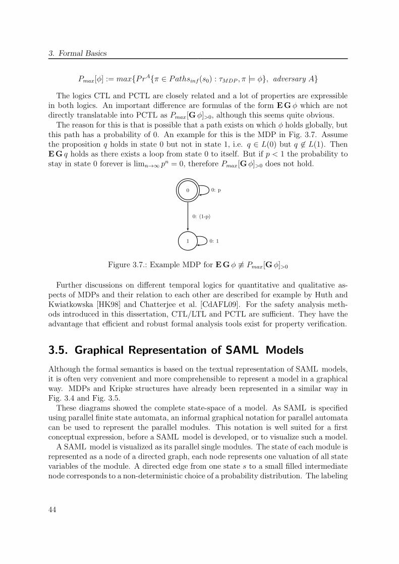
3. Formal Basics
Pmax[φ] := max{PrA{π ∈ Pathsinf(s0) : τMDP , π |= φ}, adversary A}
The logics CTL and PCTL are closely related and a lot of properties are expressiblein both logics. An important difference are formulas of the form EGφ which are notdirectly translatable into PCTL as Pmax[Gφ]>0, although this seems quite obvious.The reason for this is that is possible that a path exists on which φ holds globally, but
this path has a probability of 0. An example for this is the MDP in Fig. 3.7. Assumethe proposition q holds in state 0 but not in state 1, i.e. q ∈ L(0) but q 6∈ L(1). ThenEG q holds as there exists a loop from state 0 to itself. But if p < 1 the probability tostay in state 0 forever is limn→∞ pn = 0, therefore Pmax[Gφ]>0 does not hold.
0: (1-p)
0: 1
0: p
1
0
Figure 3.7.: Example MDP for EGφ 6≡ Pmax[Gφ]>0
Further discussions on different temporal logics for quantitative and qualitative as-pects of MDPs and their relation to each other are described for example by Huth andKwiatkowska [HK98] and Chatterjee et al. [CdAFL09]. For the safety analysis meth-ods introduced in this dissertation, CTL/LTL and PCTL are sufficient. They have theadvantage that efficient and robust formal analysis tools exist for property verification.
3.5. Graphical Representation of SAML Models
Although the formal semantics is based on the textual representation of SAML models,it is often very convenient and more comprehensible to represent a model in a graphicalway. MDPs and Kripke structures have already been represented in a similar way inFig. 3.4 and Fig. 3.5.These diagrams showed the complete state-space of a model. As SAML is specified
using parallel finite state automata, an informal graphical notation for parallel automatacan be used to represent the parallel modules. This notation is well suited for a firstconceptual expression, before a SAML model is developed, or to visualize such a model.A SAML model is visualized as its parallel single modules. The state of each module is
represented as a node of a directed graph, each node represents one valuation of all statevariables of the module. A directed edge from one state s to a small filled intermediatenode corresponds to a non-deterministic choice of a probability distribution. The labeling
44

3.6. Related Work
1
(0,0) (1,0)
(1,1)
0 1
2
case3 1
1
1
1
Module a / v_a Module b / (v_b1, v_b2)
pa
true
true
1 − pavb1 = 0 ∧ vb2 = 0
vb1 = 1 ∧ vb2 = 1
true true
true
pb3
pb2pb1
Figure 3.8.: Graphical Representation of the Example Model
of the edges is the corresponding activation condition7. The directed dashed edges froman intermediate node to a state s′ are labeled with the probability to reach the state s′
from state s.
In Fig. 3.8 the graphical representation of the SAML model of Fig. 3.2 is shown. Itconsists of the two parallel finite state modules a and b. Each possible state of a moduleis represented as a node of a directed graph. As the module a consists of only a singlestate variable, each state holds only one value. Module b consists of two state variables,its states therefore hold a vector of values of the form (v_b1, v_b2). The initial stateof a is indicated via the thicker boundary and has the value 0, the initial state of b is(0, 0). For this graphical notation it is often more convenient to use symbolic names forthe values of a state variable instead of integers. This notation will be used in many ofthe presented examples in the following chapters.
3.6. Related Work
The TopCased project is a large open source approach to build a modeling frameworkfor different modeling languages for software and systems modeling. The approach isdescribed by Vernadat et al. in [VPF+06]. Target input languages are SysML [Sys08],UML [Gro06] and the Architecture analysis and design language (AADL) [SA04]. Oneaspect of TopCased is to allow for the formal analysis of these models. The approach hereis to use the language FICARE as an intermediate language which is described by Fairailet al. [FGP+08]. Models specified in the modeling framework are then transformed intoFIACRE as intermediate language. From there models are transformed into the input
7The parts of the activation condition that refer to the values of the state variables of the currentmodule are left out. This constraint is implicitly fulfilled by the source node of an edge.
45
3. Formal Basics
language of different analysis tools like the CADP toolbox developed at INRIA anddescribed by Fernandez et al. [FGK+96] or the TINA petri net analyzer described byBerthomieu et al. in [BaFV04].
Some of the problems arising from the approach taken in the TopCased project aredescribed by Farail et al. [FGP+08]. The modeling framework provides so many modelingartifacts, that the resulting FIACRE models are often too complex for the analysis.Effectively only very small examples can be analyzed at the moment. Mainly structuralaspects can be verified. SAML has deliberately been kept as simple as possible toprevent such a situation.
Harel’s Statemate state-charts [HN96] provide a well-defined formal semantics andhave a reduced set of modeling artifacts compared to TopCased models. They cantherefore be used for qualitative formal analysis of the modeled systems. In Thums etal. [TOWS04] the interactive theorem prover KIV is used for verification. In Chan etal. [CAB+01] and Clarke and Heile [CH00], automatic model-checking techniques areused. In the AVACS [AVA03] project, Bode et al. [BPRW08a] developed a state-chartextension with probabilistic behavior and used it for safety analysis. The resultingmodel is transformed into a labeled transition system and minimized with bisimulationtechniques using the CADP [FGK+96] toolbox. The final transition system is thenanalyzed with the MRMC [KKZ05] probabilistic model-checker of Katoen et al. [KKZ05].
Maybe the most elaborate framework especially for the specification of safety-criticalsystems and model-based safety analysis is developed in the Correctness, Modeling andPerformance of Aerospace Systems (COMPASS) project [BCK+09a] described by Boz-zano et al. [BCK+10b]. It combines both qualitative and quantitative modeling capa-bilities via a formalization of a subset of AADL [SA04] and its error annex [SA06]. Thequantitative analysis is then conducted using the MRMC model checker.
The developed language is called SLIM [BCK+09b]. Models in SLIM can contain hy-brid continuous behavior, the failure modeling can contain continuous time failure rates.There is a strict discrimination between the nominal behavior (without occurrence offailures) and the failure behavior. One drawback here is that it is not possible to specifyprobabilistic nominal behavior, but only probabilistic failure behavior. Probabilistic be-havior can often be used to specify realistic environment models which is very importantfor safety analysis as safety-critical system cannot be examined in isolation. In Chapter4 the usage of probabilistic behavior in SAML to model realistic environment for bothnominal and failure behavior will be presented.
Both approaches use a continuous time model which, according to Hermanns etal. [HKMKS00], is well suited for asynchronous interleaved systems. Many safety-criticalsystems are developed using synchronous parallel components, SAML is based on dis-crete time synchronous parallel semantics. Of course, modeling asynchronicity is possiblein SAML , but must be done explicitly. In addition, probabilistic discrete time modelingis an advantage if different failure types must be modeled. This is explained in moredetail in Chapter 4.
46
3.6. Related Work
Summary
This chapter introduced the syntax and formal semantics of the SAML framework. It de-scribes synchronous parallel automata which can have a combination of non-deterministicand probabilistic transitions. This allows for the expression of both quantitative modelsand also purely qualitative ones. The underlying formal semantics are Markov DecisionProcesses (MDP). Properties are expressed as temporal logics formulas. Qualitativeproperties in LTL or CTL and quantitative properties in PCTL. Any SAML modelcan be abstracted to a purely qualitative model by the transformation into its embed-ded Kripke structure. This allows for the analysis of both qualitative and quantitativeproperties of a SAML model.
47


4. SAML Modeling for Safety Analysis
On two occasions I have been asked: “Pray, Mr.Babbage, if you put into the machine wrong figures,will the right answers come out?”I am not able rightly to apprehend the kind ofconfusion of ideas that could provoke such aquestion.
(Charles Babbage)
This chapter describes how models for safety analysis can be constructed using SAML.These models generally consist of modeling of hardware, software and the surroundingenvironment and are called extended system models. Correct environment modeling isvery important for accurate safety analysis, as the safety of a system cannot be under-stood in isolation of its surroundings. Important aspects of the environment modelingare general physical behavior and especially accurate modeling of different kinds of fail-ure modes and their effects.Section 4.1 gives a motivation for a general guideline for the creation of SAML sys-
tem models for safety analysis. Section 4.2 introduces a case study (taken from safetyanalysis literature) which will be used for illustration purposes throughout the disserta-tion and to illustrate SAML modeling for safety analysis. Section 4.3 shortly describesthe approaches for hardware and software modeling in SAML. Section 4.4 describes theapproach for realistic probabilistic environment modeling in SAML and Section 4.5 de-scribes correct and accurate failure mode modeling which is essential for safety analysis.Some related work is discussed in Section 4.6.
49

4. SAML Modeling for Safety Analysis
4.1. Motivation
To conduct a realistic model-based safety analysis, a meaningful modeling of the sys-tem under consideration is necessary. Especially if an accurate quantitative analysis isdesired, the precision of the analysis result depends heavily on the accuracy of the mod-eling. Safety analysis cannot be conducted in isolation, but the environment into whichthe system is embedded always has to be considered too, as it often strongly influencesthe possible behavior.In general, a formal system model of a software-intensive system will include software
and hardware components as well as a model of the environment. Hardware componentsare often sensors and actors that the software uses to get information about the currentenvironment and to make the system react to it. The environment model specifies thebehavior of the surroundings of the system that influence it directly or indirectly.When a model is built consisting of these aspects, it is possible to verify the functional
correctness of a system. This means that the system works as intended and fulfills itsspecification. For a safety-critical system, the analysis of functional correctness alone isnot sufficient. The assumption that all components work according to their specificationis in general wrong as different components may fail. Therefore the most importantquestion for safety analysis is:
“How safe is the system, if one or more components do not behave accordingto their specification?”
To answer this question, the potential occurrence of faulty behavior of components andalso the effects of this misbehavior must also be modeled accurately and be integratedinto the formal system model. When the faulty behavior is integrated into a SAMLmodel, it is called the extended system model. Qualitative and quantitative safetyanalyses can be conducted on an extended system model expressed in SAML. With theconstruction presented in this chapter, it is possible to integrate different types of failuremodes while preserving the functional correctness of the system model.Fig. 4.1 shows the general structure of an extended system model for model-based
safety analysis. The software model interacts with the hardware model, reading andprocessing inputs and emitting control commands. The interaction of the software withthe environment is generally indirectly via the hardware model. Actors and sensorsare influenced by the physical environment model. All hardware components can beinfluenced by the occurrence of component failures and their effects specified by thefailure model.Very often there will not be a one-to-one correspondence between SAML modules
and one of these aspects. But on the conceptual level, all those aspects are required foran accurate model-based safety analysis. This allows for giving some general modelingguidelines for both environmental and failure mode modeling in SAML which will oftenbe helpful in the analysis of safety critical systems.
50
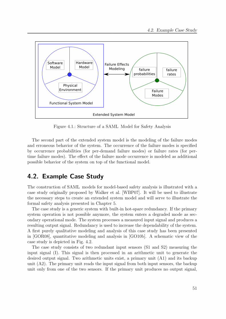
4.2. Example Case Study
Software
Model
Physical
Environment Failure
Modes
Hardware
Model
Functional System Model
failure
probabilitiesfailure
rates
Extended System Model
Failure Effects
Modeling
Figure 4.1.: Structure of a SAML Model for Safety Analysis
The second part of the extended system model is the modeling of the failure modesand erroneous behavior of the system. The occurrence of the failure modes is specifiedby occurrence probabilities (for per-demand failure modes) or failure rates (for per-time failure modes). The effect of the failure mode occurrence is modeled as additionalpossible behavior of the system on top of the functional model.
4.2. Example Case Study
The construction of SAML models for model-based safety analysis is illustrated with acase study originally proposed by Walker et al. [WBP07]. It will be used to illustratethe necessary steps to create an extended system model and will serve to illustrate theformal safety analysis presented in Chapter 5.The case study is a generic system with built-in hot-spare redundancy. If the primary
system operation is not possible anymore, the system enters a degraded mode as sec-ondary operational mode. The system processes a measured input signal and produces aresulting output signal. Redundancy is used to increase the dependability of the system.A first purely qualitative modeling and analysis of this case study has been presentedin [GOR08], quantitative modeling and analysis in [GO10b]. A schematic view of thecase study is depicted in Fig. 4.2.The case study consists of two redundant input sensors (S1 and S2) measuring the
input signal (I). This signal is then processed in an arithmetic unit to generate thedesired output signal. Two arithmetic units exist, a primary unit (A1) and its backupunit (A2). The primary unit reads the input signal from both input sensors, the backupunit only from one of the two sensors. If the primary unit produces no output signal,
51

4. SAML Modeling for Safety Analysis
M
S1
A1
O
A2
S2
I
Figure 4.2.: Schematic View of Example Case Study [GOR08]
then a monitoring unit (M) switches to the backup unit for the generation of the outputsignal. The backup unit will only produce an output signal if it has been triggered bythe monitor. If the secondary unit is triggered, the primary unit will get switched off.The system is functionally correct if it delivers a correct output signal. It is easy to
imagine that if such a system is used in a safety-critical environment, a malfunctioning(omission of values) could be very dangerous and the system can become safety-critical.Therefore the redundancy and the degraded mode have been integrated.
4.3. Hardware and Software Modeling
For safety analysis, the first step is to construct a model of the functional behavior ofthe system. This functional system model specifies the intended behavior of the systemunder consideration and is used to verify the functional correctness of the system, provingthat it works as intended. The modeling of hardware and software forms the basis forsuch functional formal models expressed in SAML. It defines the basic behavior of themodeled system and its reaction to and its influence on its surrounding environment. Toget the most accurate analysis results, it is important to analyze a system model whichbehaves as similar as possible as the system under consideration.
4.3.1. Software Modeling
For formal model-based safety analysis, most often software will be specified in an ab-stract way. Not every detail of the algorithms will be modeled, only the most importantconcepts. The reason for this is firstly the fact that fine-grained software specificationswould increase the state space enormously, making an analysis very difficult or evenimpossible. Secondly, the correctness of the algorithms and the software specificationcan better be assured using other techniques than model-checking, e.g. interactive the-orem proving, as this is often undecidable or requires infinite state spaces. Thirdly and
52

4.3. Hardware and Software Modeling
most important, the main interest in safety analysis is the combination of hardware,software and its behavior in a (possibly failing) environment. For such an analysis theimplementation details are not of interest, but only the important effects1 of the im-plemented software. Therefore abstract specifications of software are generally used inSAML models which show primarily these intended effects.
4.3.2. Hardware Modeling
The hardware model of a formal SAML model will most often represent the interfaceof the system under consideration to its surrounding physical environment. This typi-cally consists of sensors and actors. Sensors are used to get feedback from the physicalenvironment of the system. Depending on this feedback, the system changes its internalstate according to its software specification. Actuators are then used to influence theenvironment according to the changed system state.Depending on the system under consideration, the hardware model may also consist
of additional aspects. Examples for this are aspects which define the spatial structureof a system and therefore the possible interactions of different components. Other pos-sible aspects are for example general technical modeling of aspects like communicationchannels and component interfaces.
4.3.3. Case Study Model
One component of the example case study which reads input from hardware (sensors)and acts according to a (simple) software specification is the model of the secondaryarithmetic unit (A2). Its modeling is shown in Fig. 4.3. Initially it is in state idle, i.e.a hot stand-by state where no output is produced. It stays in this state until it getsactivated (predicate activate is true) by the monitoring unit. It then is in state sig,as long as there is data available (the predicate signal holds which means sensor S2produces data). If there is no data available, the unit enters the state noSig, as no signalcan be produced. If the sensor starts delivering data again, A2 switches back to statesig. Here the software controls the different states of the A2 unit, the hardware modelconsists of the sensors that deliver the data and the production of the output signal ofthe system from the arithmetic units.The whole functional system model of the case study consists of 5 parallel SAML
modules. One for each of the two sensors that indicates whether the sensor delivers asignal, one for the primary arithmetic (A1) unit and one for the monitoring unit thatdetects when A1 fails to deliver a signal and activates A2. The functional system modelis then the parallel composition of these five SAML modules. The functional correctnessof the system can be verified by proving that there is always an output signal producedonce the system enters its normal operating mode.
1Most often the change of the internal state of the system.
53

4. SAML Modeling for Safety Analysis
Module arith2 / arith2
idle noSig1
1
1
¬signal
1
¬signal
signal
1
signal
¬activate
activate
sig
Figure 4.3.: SAML Module of Second Arithmetic Unit
4.4. Physical Environment Modeling
The accuracy of the physical environment modeling is very important for the accuracyof the analysis of a SAML model. Physical behavior can often be described in waysof measurable units and the rate of change of these units. In mathematical terms,measurable units are described as functions and the rate of change of these units isdescribed as the derivations of these functions. An often used example of this in physicalenvironment modeling is the function from time to space which describes the position at agiven time. Its derivation is the velocity and its second derivation is the acceleration (foran example using this type of environment modeling see Section 7.1). Other physicalbehavior can often be modeled analogously, but it is important to note that SAMLmodels are discrete and values can only use finite domains, so all continuous values haveto be discretized.
4.4.1. Temporal Resolution
To model physical behavior realistically, the correct interpretation of the passing of timeand its correct integration into the model is of biggest importance. In SAML, a discretetime model is used. In such a context, there exists a basic time unit which passeswhenever the system performs a step (i.e. all parallel finite state machines execute anupdate rule).This means that whenever the state variables change, the same amount of time passes
for all modules. This basic unit is called the temporal resolution ∆t of the system.In synchronous parallel systems this will usually be a basic system clock2. All time-
2This basic system clock is not equal to the CPU clock of a system, but most often a (large) multiplethereof.
54
4.5. Failure Mode Modeling
dependent SAML modeling, physical behavior modeling of the environment model andespecially the failure mode modeling is done relative to ∆t.
Definition 25. Temporal Resolution of a SAML model
The amount of time ∆t that passes at each time-step of a SAML model is called thetemporal resolution. In general its unit is given in seconds or fractions thereof.
The value of ∆t is very much system-dependent. As it defines the basic system clock,it must be chosen accordingly to the abstraction level of the software and hardwaremodeling (e.g. the sensor reading frequency). Some discussion on the effect of ∆t fora formal system model is presented in Section 4.5.2 on formal failure modeling and inSection 5.3.3 on the interpretation of quantitative analysis results.
4.4.2. Case Study Model
In the functional system model of the case study, the core aspect of the physical modelingis the frequency that input signals are read, processed and sent to the output. Thetemporal resolution of the system is modeled as ∆t = 10ms, which means that thesignal frequency is 100Hz. The frequency of the hardware in the processing units of A1and A2 would of course be higher, but as already mentioned, ∆t does not necessarilycorrespond to the CPU clock of the system but is an abstract basic clock.
4.5. Failure Mode Modeling
After the construction of the functional system model and the modeling of the physicalenvironment, the most important step from the point of model-based safety analysis isconducted: the accurate modeling of the failure modes. The basic idea is to integratethe effect of the failure mode occurrence into the functional model. It is important todo this in such a way, that the original behavior is still retained. For the formal modelthis means that the functional correctness of the system model is retained although itis extended with possible defective behavior. This assures that the later safety analysisreflects properly the behavior of the system under consideration in the case of compo-nent failures. This makes the presented modeling and integration of the failure modesconservative. This concept was introduced by Ortmeier et al. in [ORS05], some exten-sions can be found in [OGR07]. But until now this integration was limited to purelyqualitative failure mode modeling.
The identification of possible failure modes for a given system is not discussed here,the existence of a set of relevant failure modes is assumed. Such a set is often givendirectly for components for which the possible failure modes are known. Methods tosystematically find possible failure modes can also be applied, for example HaZop asdescribed by Kletz [Kle86].
55
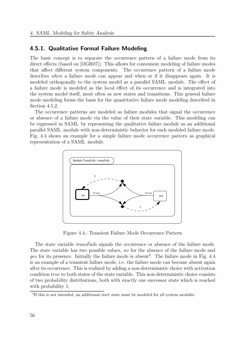
4. SAML Modeling for Safety Analysis
4.5.1. Qualitative Formal Failure Modeling
The basic concept is to separate the occurrence pattern of a failure mode from itsdirect effects (based on [OGR07]). This allows for convenient modeling of failure modesthat affect different system components. The occurrence pattern of a failure modedescribes when a failure mode can appear and when or if it disappears again. It ismodeled orthogonally to the system model as a parallel SAML module. The effect ofa failure mode is modeled as the local effect of its occurrence and is integrated intothe system model itself, most often as new states and transitions. This general failuremode modeling forms the basis for the quantitative failure mode modeling described inSection 4.5.2.The occurrence patterns are modeled as failure modules that signal the occurrence
or absence of a failure mode via the value of their state variable. This modeling canbe expressed in SAML by representing the qualitative failure module as an additionalparallel SAML module with non-deterministic behavior for each modeled failure mode.Fig. 4.4 shows an example for a simple failure mode occurrence pattern as graphicalrepresentation of a SAML module.
Module TransFails / transFails
no yes
1
true true
1
Figure 4.4.: Transient Failure Mode Occurrence Pattern
The state variable transFails signals the occurrence or absence of the failure mode.The state variable has two possible values, no for the absence of the failure mode andyes for its presence. Initially the failure mode is absent3. The failure mode in Fig. 4.4is an example of a transient failure mode, i.e. the failure mode can become absent againafter its occurrence. This is realized by adding a non-deterministic choice with activationcondition true to both states of the state variable. This non-deterministic choice consistsof two probability distributions, both with exactly one successor state which is reachedwith probability 1.
3If this is not intended, an additional start state must be modeled for all system modules
56
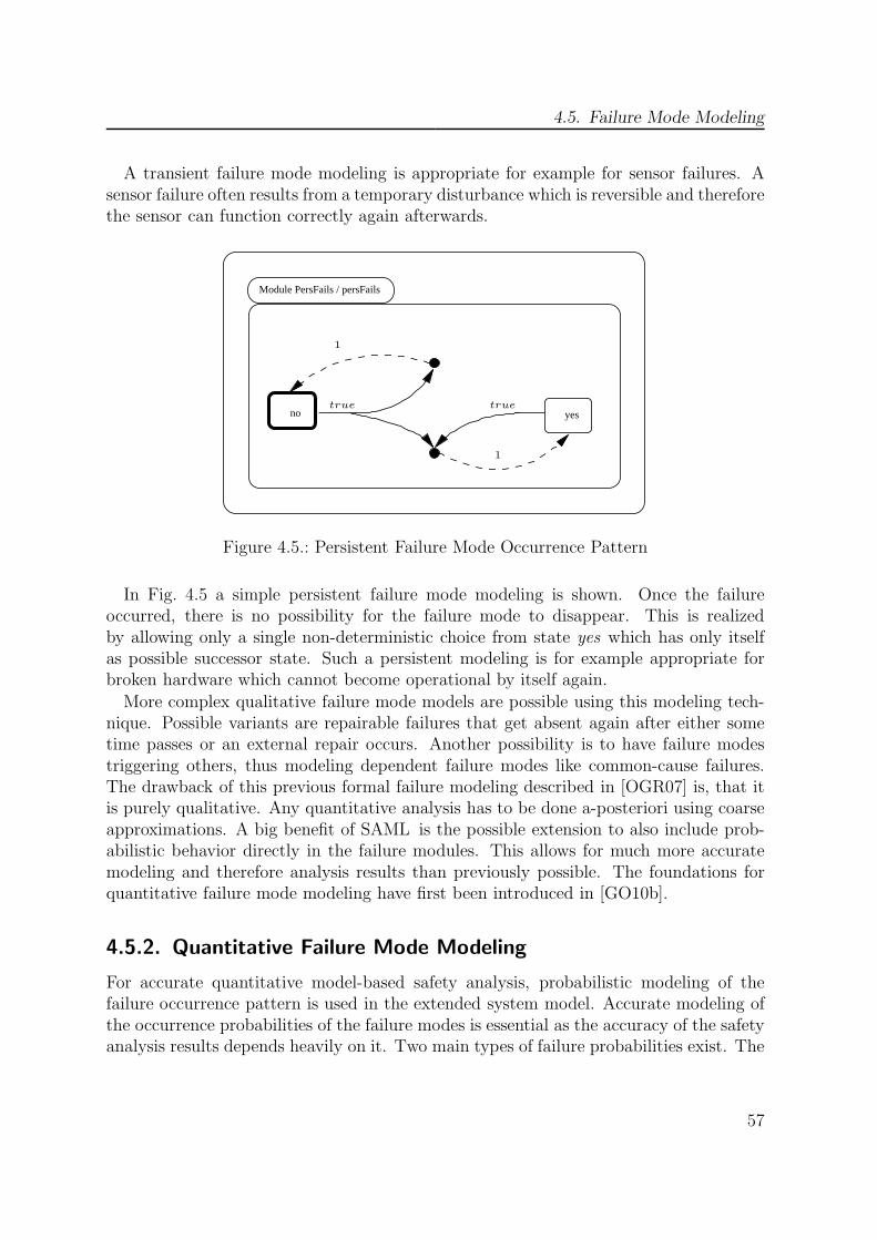
4.5. Failure Mode Modeling
A transient failure mode modeling is appropriate for example for sensor failures. Asensor failure often results from a temporary disturbance which is reversible and thereforethe sensor can function correctly again afterwards.
yes
Module PersFails / persFails
no
1
true true
1
Figure 4.5.: Persistent Failure Mode Occurrence Pattern
In Fig. 4.5 a simple persistent failure mode modeling is shown. Once the failureoccurred, there is no possibility for the failure mode to disappear. This is realizedby allowing only a single non-deterministic choice from state yes which has only itselfas possible successor state. Such a persistent modeling is for example appropriate forbroken hardware which cannot become operational by itself again.
More complex qualitative failure mode models are possible using this modeling tech-nique. Possible variants are repairable failures that get absent again after either sometime passes or an external repair occurs. Another possibility is to have failure modestriggering others, thus modeling dependent failure modes like common-cause failures.The drawback of this previous formal failure modeling described in [OGR07] is, that itis purely qualitative. Any quantitative analysis has to be done a-posteriori using coarseapproximations. A big benefit of SAML is the possible extension to also include prob-abilistic behavior directly in the failure modules. This allows for much more accuratemodeling and therefore analysis results than previously possible. The foundations forquantitative failure mode modeling have first been introduced in [GO10b].
4.5.2. Quantitative Failure Mode Modeling
For accurate quantitative model-based safety analysis, probabilistic modeling of thefailure occurrence pattern is used in the extended system model. Accurate modeling ofthe occurrence probabilities of the failure modes is essential as the accuracy of the safetyanalysis results depends heavily on it. Two main types of failure probabilities exist. The
57
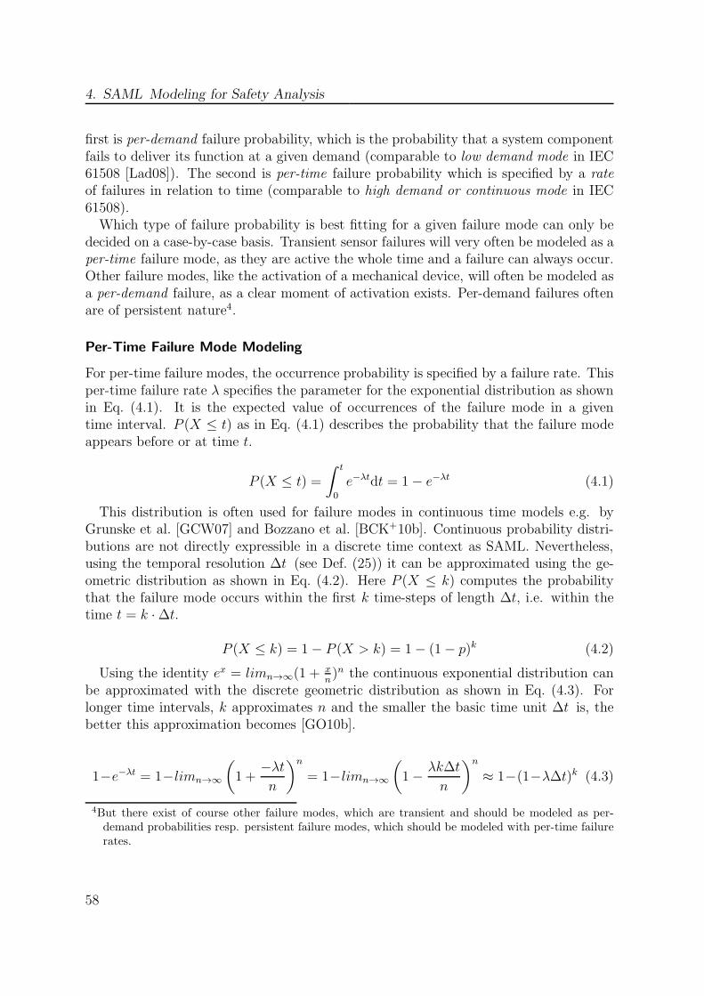
4. SAML Modeling for Safety Analysis
first is per-demand failure probability, which is the probability that a system componentfails to deliver its function at a given demand (comparable to low demand mode in IEC61508 [Lad08]). The second is per-time failure probability which is specified by a rateof failures in relation to time (comparable to high demand or continuous mode in IEC61508).Which type of failure probability is best fitting for a given failure mode can only be
decided on a case-by-case basis. Transient sensor failures will very often be modeled as aper-time failure mode, as they are active the whole time and a failure can always occur.Other failure modes, like the activation of a mechanical device, will often be modeled asa per-demand failure, as a clear moment of activation exists. Per-demand failures oftenare of persistent nature4.
Per-Time Failure Mode Modeling
For per-time failure modes, the occurrence probability is specified by a failure rate. Thisper-time failure rate λ specifies the parameter for the exponential distribution as shownin Eq. (4.1). It is the expected value of occurrences of the failure mode in a giventime interval. P (X ≤ t) as in Eq. (4.1) describes the probability that the failure modeappears before or at time t.
P (X ≤ t) =
∫ t
0
e−λtdt = 1− e−λt (4.1)
This distribution is often used for failure modes in continuous time models e.g. byGrunske et al. [GCW07] and Bozzano et al. [BCK+10b]. Continuous probability distri-butions are not directly expressible in a discrete time context as SAML. Nevertheless,using the temporal resolution ∆t (see Def. (25)) it can be approximated using the ge-ometric distribution as shown in Eq. (4.2). Here P (X ≤ k) computes the probabilitythat the failure mode occurs within the first k time-steps of length ∆t, i.e. within thetime t = k ·∆t.
P (X ≤ k) = 1− P (X > k) = 1− (1− p)k (4.2)
Using the identity ex = limn→∞(1 + xn)n the continuous exponential distribution can
be approximated with the discrete geometric distribution as shown in Eq. (4.3). Forlonger time intervals, k approximates n and the smaller the basic time unit ∆t is, thebetter this approximation becomes [GO10b].
1−e−λt = 1−limn→∞
(
1 +−λt
n
)n
= 1−limn→∞
(
1−λk∆t
n
)n
≈ 1−(1−λ∆t)k (4.3)
4But there exist of course other failure modes, which are transient and should be modeled as per-demand probabilities resp. persistent failure modes, which should be modeled with per-time failurerates.
58
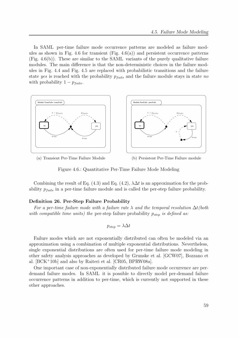
4.5. Failure Mode Modeling
In SAML per-time failure mode occurrence patterns are modeled as failure mod-ules as shown in Fig. 4.6 for transient (Fig. 4.6(a)) and persistent occurrence patterns(Fig. 4.6(b)). These are similar to the SAML variants of the purely qualitative failuremodules. The main difference is that the non-deterministic choices in the failure mod-ules in Fig. 4.4 and Fig. 4.5 are replaced with probabilistic transitions and the failurestate yes is reached with the probability pfails and the failure module stays in state nowith probability 1− pfails.
Module TransFails / transFails
no yes
pfails
truetrue
1 − pfails
(a) Transient Per-Time Failure Module
no yes
Module PersFails / persFails
pfails
truetrue
1
1 − pfails
(b) Persistent Per-Time Failure module
Figure 4.6.: Quantitative Per-Time Failure Mode Modeling
Combining the result of Eq. (4.3) and Eq. (4.2), λ∆t is an approximation for the prob-ability pfails in a per-time failure module and is called the per-step failure probability.
Definition 26. Per-Step Failure Probability
For a per-time failure mode with a failure rate λ and the temporal resolution ∆t(bothwith compatible time units) the per-step failure probability pstep is defined as:
pstep = λ∆t
Failure modes which are not exponentially distributed can often be modeled via anapproximation using a combination of multiple exponential distributions. Nevertheless,single exponential distributions are often used for per-time failure mode modeling inother safety analysis approaches as developed by Grunske et al. [GCW07], Bozzano etal. [BCK+10b] and also by Raiteri et al. [CR05, BPRW08a].
One important case of non-exponentially distributed failure mode occurrence are per-demand failure modes. In SAML it is possible to directly model per-demand failureoccurrence patterns in addition to per-time, which is currently not supported in theseother approaches.
59
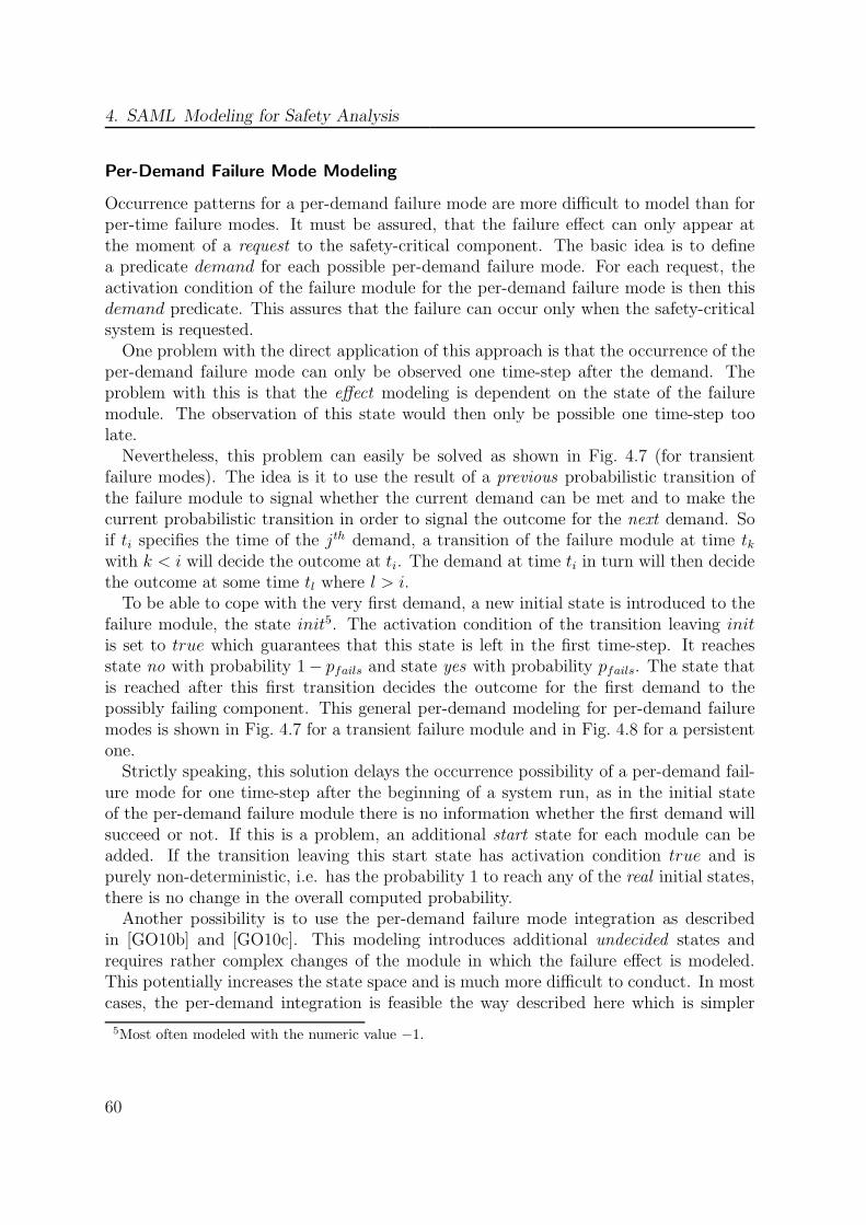
4. SAML Modeling for Safety Analysis
Per-Demand Failure Mode Modeling
Occurrence patterns for a per-demand failure mode are more difficult to model than forper-time failure modes. It must be assured, that the failure effect can only appear atthe moment of a request to the safety-critical component. The basic idea is to definea predicate demand for each possible per-demand failure mode. For each request, theactivation condition of the failure module for the per-demand failure mode is then thisdemand predicate. This assures that the failure can occur only when the safety-criticalsystem is requested.One problem with the direct application of this approach is that the occurrence of the
per-demand failure mode can only be observed one time-step after the demand. Theproblem with this is that the effect modeling is dependent on the state of the failuremodule. The observation of this state would then only be possible one time-step toolate.Nevertheless, this problem can easily be solved as shown in Fig. 4.7 (for transient
failure modes). The idea is it to use the result of a previous probabilistic transition ofthe failure module to signal whether the current demand can be met and to make thecurrent probabilistic transition in order to signal the outcome for the next demand. Soif ti specifies the time of the jth demand, a transition of the failure module at time tkwith k < i will decide the outcome at ti. The demand at time ti in turn will then decidethe outcome at some time tl where l > i.To be able to cope with the very first demand, a new initial state is introduced to the
failure module, the state init5. The activation condition of the transition leaving initis set to true which guarantees that this state is left in the first time-step. It reachesstate no with probability 1− pfails and state yes with probability pfails. The state thatis reached after this first transition decides the outcome for the first demand to thepossibly failing component. This general per-demand modeling for per-demand failuremodes is shown in Fig. 4.7 for a transient failure module and in Fig. 4.8 for a persistentone.Strictly speaking, this solution delays the occurrence possibility of a per-demand fail-
ure mode for one time-step after the beginning of a system run, as in the initial stateof the per-demand failure module there is no information whether the first demand willsucceed or not. If this is a problem, an additional start state for each module can beadded. If the transition leaving this start state has activation condition true and ispurely non-deterministic, i.e. has the probability 1 to reach any of the real initial states,there is no change in the overall computed probability.Another possibility is to use the per-demand failure mode integration as described
in [GO10b] and [GO10c]. This modeling introduces additional undecided states andrequires rather complex changes of the module in which the failure effect is modeled.This potentially increases the state space and is much more difficult to conduct. In mostcases, the per-demand integration is feasible the way described here which is simpler
5Most often modeled with the numeric value −1.
60

4.5. Failure Mode Modeling
Module TransDemand / transDemand
no yes
init
1
¬demand
¬demand
1
demanddemand
true
1 − pfails pfails
Figure 4.7.: Transient Per-Demand Failure Automaton
Module PersDemand / persDemand
no yes
init
1
¬demand
1
demand
true
true
pfails1 − pfails
Figure 4.8.: Persistent Per-Demand Failure Automaton
than the outlined alternatives. Note, that this is a similar design choice to make for theper-time failure mode modeling, where the failure modules are generally modeled withno as initial state.
Case Study Model
These two different kinds of failure occurrence patterns are used for the modeling of thecase study. A variety of failures modes is possible, it is assumed that a list of the relevantfailure modes exists. The ones considered in the modeling and analysis are the following:
61

4. SAML Modeling for Safety Analysis
The sensors can omit a signal (S1FailsSig, S2FailsSig), making it impossible for one ofthe arithmetic units to process the data from the sensors correctly. The arithmetic unitsthemselves can omit producing output data (A1FailsSig, A2FailsSig). The monitorcan fail to detect that situation (MonitorFails), either switching if not necessary or notswitching if necessary. The activation of the A2 unit may fail (A2FailsActivate) althoughthe monitor sent the activation signal to A2. The failure occurrence patterns for thesesix failure modes are integrated into the SAML model of the case study for its safetyanalysis.
no yes
Module MonitorFails / monitorfails
truetrue
1 − pMonitorFails pMonitorFails
Figure 4.9.: MonitorFails Failure Occurrence Pattern
Example of a Per-Time Failure Mode As an example of a per-time failure mode, themodeling of the transient failure mode MonitorFails is presented. The per-time failuremodule is shown in Fig. 4.9. At any system step, the failure may appear or disappeardepending on its per-step probability pMonitorFails.The failure rate for the MonitorFails is assumed to be λMonitorFails = 1 · 10−6 1
hwhich
translates to a per-step probability of pMonitorFails = 2.7778 · 10−12 for ∆t = 10ms.The approximation errors for this per-time failure mode are shown in Fig. 4.10. in twotime-vs-error (time in ms) plots. The absolute approximation error
ǫabs(t) := |(1− e−λt)− (1− (1− λ∆t)k)|
in Fig. 4.10(a), the relative approximation error
ǫrel(t) := |ǫabs(t)
1− e−λt|
is shown in Fig. 4.10(b). Both decrease for longer run-times as expected from Eq. (4.3).
62
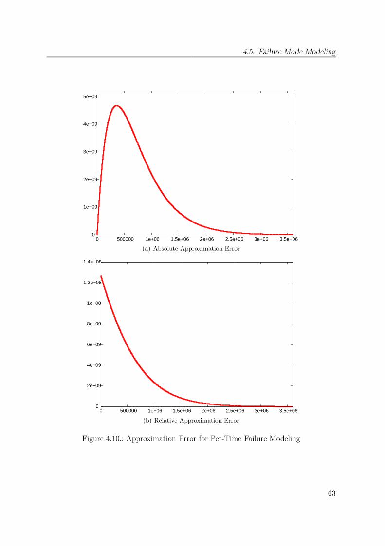
4.5. Failure Mode Modeling
0
1e−09
2e−09
3e−09
4e−09
5e−09
0 500000 1e+06 1.5e+06 2e+06 2.5e+06 3e+06 3.5e+06
(a) Absolute Approximation Error
0
2e−09
4e−09
6e−09
8e−09
1e−08
1.2e−08
1.4e−08
0 500000 1e+06 1.5e+06 2e+06 2.5e+06 3e+06 3.5e+06
(b) Relative Approximation Error
Figure 4.10.: Approximation Error for Per-Time Failure Modeling
63

4. SAML Modeling for Safety Analysis
Example of a Per-Demand Failure Mode The failure mode A2FailsActivate, thefailure to activate the A2 unit if required, can only appear if there is a request fromthe monitor and is therefore modeled as a per-demand failure mode. The correspondingfailure module can be seen in Fig. 4.11. The predicate demand is defined as arith2 =idle∧activate, i.e. the backup arithmetic unit is in its idle state and should be activatedbecause A1 does not deliver any more signal (predicate activate holds). The per-demandoccurrence probability of this failure mode is modeled as 1 · 10−7.
Module a2failsActivate / a2failsActivate
no yes
init
11
true
true
1 − pfails pfails
activate
arith2 = idle∧
activate)
¬(arith2 = idle∧
Figure 4.11.: A2FailsActivate Failure Occurrence Pattern
Additional Failure Modes For the analysis of the complete case study, the failuremodules for the four remaining failure modes are also modeled. S2FailsSig is modeled asa per-time failure mode analogous to S1FailsSig, both with a failure rate of λS1FailsSig =1 · 10−2 1
h. The failure modes A2FailsSig, A1FailsSig are modeled as per-time failure
modes. The failure rate for A2FailsSig is also 1 · 10−2 1h, the failure rate for A1FailsSig
is 1 · 10−6 1h, as it is assumed that the primary unit A1 is of better quality than the
secondary unit. With a temporal resolution ∆t = 10ms, this translates to a per-stepfailure probability of 2.7778 · 10−8 for the failure rates 1 · 10−2 1
hand 2.7778 · 10−12 for
the failure rates 1 · 10−6 1h.
The modeling presented here only defines the various occurrence patterns and there-fore when a certain failure mode can occur and how probable that is. This forms thefoundation of the modeling of the effects of the occurrence of the failure modes, i.e. whathappens if the failure mode occurs.
64
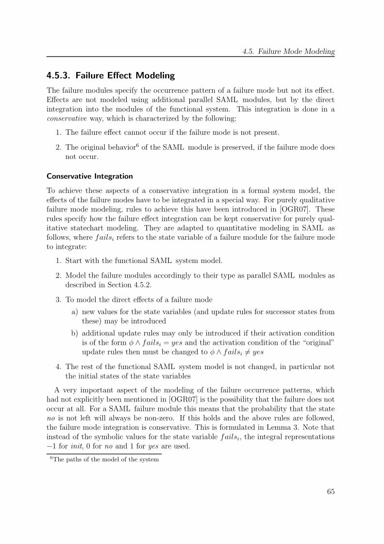
4.5. Failure Mode Modeling
4.5.3. Failure Effect Modeling
The failure modules specify the occurrence pattern of a failure mode but not its effect.Effects are not modeled using additional parallel SAML modules, but by the directintegration into the modules of the functional system. This integration is done in aconservative way, which is characterized by the following:
1. The failure effect cannot occur if the failure mode is not present.
2. The original behavior6 of the SAML module is preserved, if the failure mode doesnot occur.
Conservative Integration
To achieve these aspects of a conservative integration in a formal system model, theeffects of the failure modes have to be integrated in a special way. For purely qualitativefailure mode modeling, rules to achieve this have been introduced in [OGR07]. Theserules specify how the failure effect integration can be kept conservative for purely qual-itative statechart modeling. They are adapted to quantitative modeling in SAML asfollows, where failsi refers to the state variable of a failure module for the failure modeto integrate:
1. Start with the functional SAML system model.
2. Model the failure modules accordingly to their type as parallel SAML modules asdescribed in Section 4.5.2.
3. To model the direct effects of a failure mode
a) new values for the state variables (and update rules for successor states fromthese) may be introduced
b) additional update rules may only be introduced if their activation conditionis of the form φ ∧ failsi = yes and the activation condition of the “original”update rules then must be changed to φ ∧ failsi 6= yes
4. The rest of the functional SAML system model is not changed, in particular notthe initial states of the state variables
A very important aspect of the modeling of the failure occurrence patterns, whichhad not explicitly been mentioned in [OGR07] is the possibility that the failure does notoccur at all. For a SAML failure module this means that the probability that the stateno is not left will always be non-zero. If this holds and the above rules are followed,the failure mode integration is conservative. This is formulated in Lemma 3. Note thatinstead of the symbolic values for the state variable failsi, the integral representations−1 for init, 0 for no and 1 for yes are used.
6The paths of the model of the system
65

4. SAML Modeling for Safety Analysis
Lemma 3. Conservative Integration
Let M be a SAML model with the set of state variables V ar and M ′ be the SAMLmodel in which the effect of a failure mode γi is integrated into M adhering to the rulesabove. Let Fi be the corresponding failure module, failsi the state variable that indicatesthat the failure mode is absent (failsi ≤ 0) or present (failsi > 0). Let τMDP be theMDP corresponding to M and τ ′MDP be the MDP corresponding to M ′||Fi. Then:
∀π ∈ Paths(κ(τMDP )) : ∃π′ ∈ Paths(κ(τ ′MDP )) : π ≡ π′|V ar (4.4)
where π′|V ar is the projection of π′ onto the state variables v ∈ V ar
proof see p. 168
It is important to note that this notion of conservative integration applies only to thepresence of the same paths and traces. Typically the probabilities will change by theintroduction of the failure mode modeling, as this modeling is probabilistic. In generalthis is not a problem, as the relation of the probabilities in the original model and theequivalent paths in the extended system model is not changed.
If more than one failure mode is integrated into the model, there exists the possibilitythat the modeling of effects of one failure mode γi is masked by the modeling of theeffects of another failure mode γj. This situation can be resolved at modeling time byspecifying a priority on the failure modes, e.g. always first considering γi before γi.Another possibility to cope with this situation is to use non-deterministic modeling insuch a way that the adversary resolves this situation at the time of the analysis. Whichapproach is better depends on the nature of the modeled system and on the amount ofinformation on the failure effect that is available.
Lemma 3 also applies to the successive integration of all failure modes. This meansthat each successive integration is conservative. Therefore the original behavior of thesystem model is still possible after each of the failure mode occurrence patterns andfailure mode effects modeling is integrated. The resulting SAML model in which allfailure modes are integrated conservatively, is called the extended system model. If non-deterministic modeling is used or the priority of failure effects modeling is always thesame, then all possible orderings of conservative failure effect integration as describedabove produce isomorphic extended system models.
Definition 27. Extended System Model
Let M be a functional SAML model, ∆ the set of failure modes γi with correspondingfailure module Fi and (M ′)i the conservative integration of the failure mode γi into themodel M ′ adhering to the construction rules. Then ((M)1 . . .)n||F1|| · · · ||Fn is called theextended system model M+.
66
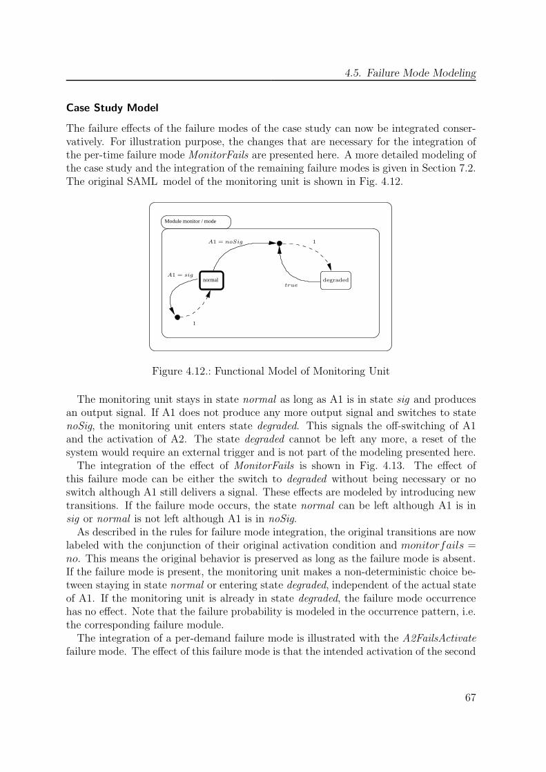
4.5. Failure Mode Modeling
Case Study Model
The failure effects of the failure modes of the case study can now be integrated conser-vatively. For illustration purpose, the changes that are necessary for the integration ofthe per-time failure mode MonitorFails are presented here. A more detailed modeling ofthe case study and the integration of the remaining failure modes is given in Section 7.2.The original SAML model of the monitoring unit is shown in Fig. 4.12.
Module monitor / mode
normalA1 = sig
1
degradedtrue
1
A1 = noSig
Figure 4.12.: Functional Model of Monitoring Unit
The monitoring unit stays in state normal as long as A1 is in state sig and producesan output signal. If A1 does not produce any more output signal and switches to statenoSig, the monitoring unit enters state degraded. This signals the off-switching of A1and the activation of A2. The state degraded cannot be left any more, a reset of thesystem would require an external trigger and is not part of the modeling presented here.The integration of the effect of MonitorFails is shown in Fig. 4.13. The effect of
this failure mode can be either the switch to degraded without being necessary or noswitch although A1 still delivers a signal. These effects are modeled by introducing newtransitions. If the failure mode occurs, the state normal can be left although A1 is insig or normal is not left although A1 is in noSig.As described in the rules for failure mode integration, the original transitions are now
labeled with the conjunction of their original activation condition and monitorfails =no. This means the original behavior is preserved as long as the failure mode is absent.If the failure mode is present, the monitoring unit makes a non-deterministic choice be-tween staying in state normal or entering state degraded, independent of the actual stateof A1. If the monitoring unit is already in state degraded, the failure mode occurrencehas no effect. Note that the failure probability is modeled in the occurrence pattern, i.e.the corresponding failure module.The integration of a per-demand failure mode is illustrated with the A2FailsActivate
failure mode. The effect of this failure mode is that the intended activation of the second
67
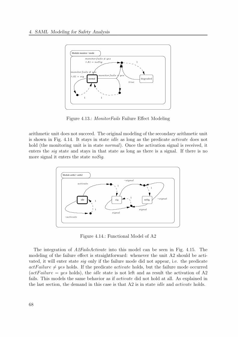
4. SAML Modeling for Safety Analysis
Module monitor / mode
normal
1
degraded
1
monitorfails = yes
∧A1 = noSig
∧A1 = sig
1
true
monitorfails 6= yes
monitorfails 6= yes
Figure 4.13.: MonitorFails Failure Effect Modeling
arithmetic unit does not succeed. The original modeling of the secondary arithmetic unitis shown in Fig. 4.14. It stays in state idle as long as the predicate activate does nothold (the monitoring unit is in state normal). Once the activation signal is received, itenters the sig state and stays in that state as long as there is a signal. If there is nomore signal it enters the state noSig.
Module arith2 / arith2
idle noSig1
1
1
¬signal
1
¬signal
signal
1
signal
¬activate
activate
sig
Figure 4.14.: Functional Model of A2
The integration of A2FailsActivate into this model can be seen in Fig. 4.15. Themodeling of the failure effect is straightforward: whenever the unit A2 should be acti-vated, it will enter state sig only if the failure mode did not appear, i.e. the predicateactFailure 6= yes holds. If the predicate activate holds, but the failure mode occurred(actFailure = yes holds), the idle state is not left and as result the activation of A2fails. This models the same behavior as if activate did not hold at all. As explained inthe last section, the demand in this case is that A2 is in state idle and activate holds.
68
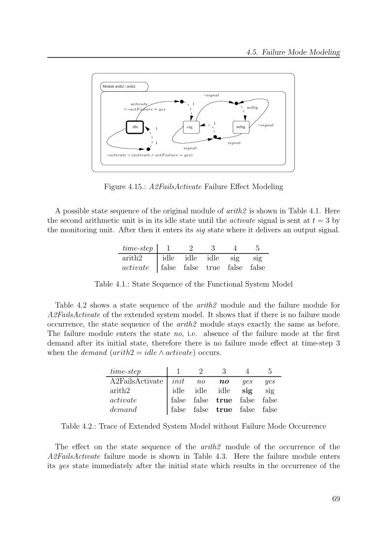
4.5. Failure Mode Modeling
Module arith2 / arith2
idle noSig1
1
1
¬signal
¬signal
signal
1
signal
activate
sig
noSig
¬activate∨ (activate ∧ actFailure = yes)
∧¬actFailure = yes
Figure 4.15.: A2FailsActivate Failure Effect Modeling
A possible state sequence of the original module of arith2 is shown in Table 4.1. Herethe second arithmetic unit is in its idle state until the activate signal is sent at t = 3 bythe monitoring unit. After then it enters its sig state where it delivers an output signal.
time-step 1 2 3 4 5arith2 idle idle idle sig sigactivate false false true false false
Table 4.1.: State Sequence of the Functional System Model
Table 4.2 shows a state sequence of the arith2 module and the failure module forA2FailsActivate of the extended system model. It shows that if there is no failure modeoccurrence, the state sequence of the arith2 module stays exactly the same as before.The failure module enters the state no, i.e. absence of the failure mode at the firstdemand after its initial state, therefore there is no failure mode effect at time-step 3when the demand (arith2 = idle ∧ activate) occurs.
time-step 1 2 3 4 5A2FailsActivate init no no yes yesarith2 idle idle idle sig sigactivate false false true false falsedemand false false true false false
Table 4.2.: Trace of Extended System Model without Failure Mode Occurrence
The effect on the state sequence of the arith2 module of the occurrence of theA2FailsActivate failure mode is shown in Table 4.3. Here the failure module entersits yes state immediately after the initial state which results in the occurrence of the
69
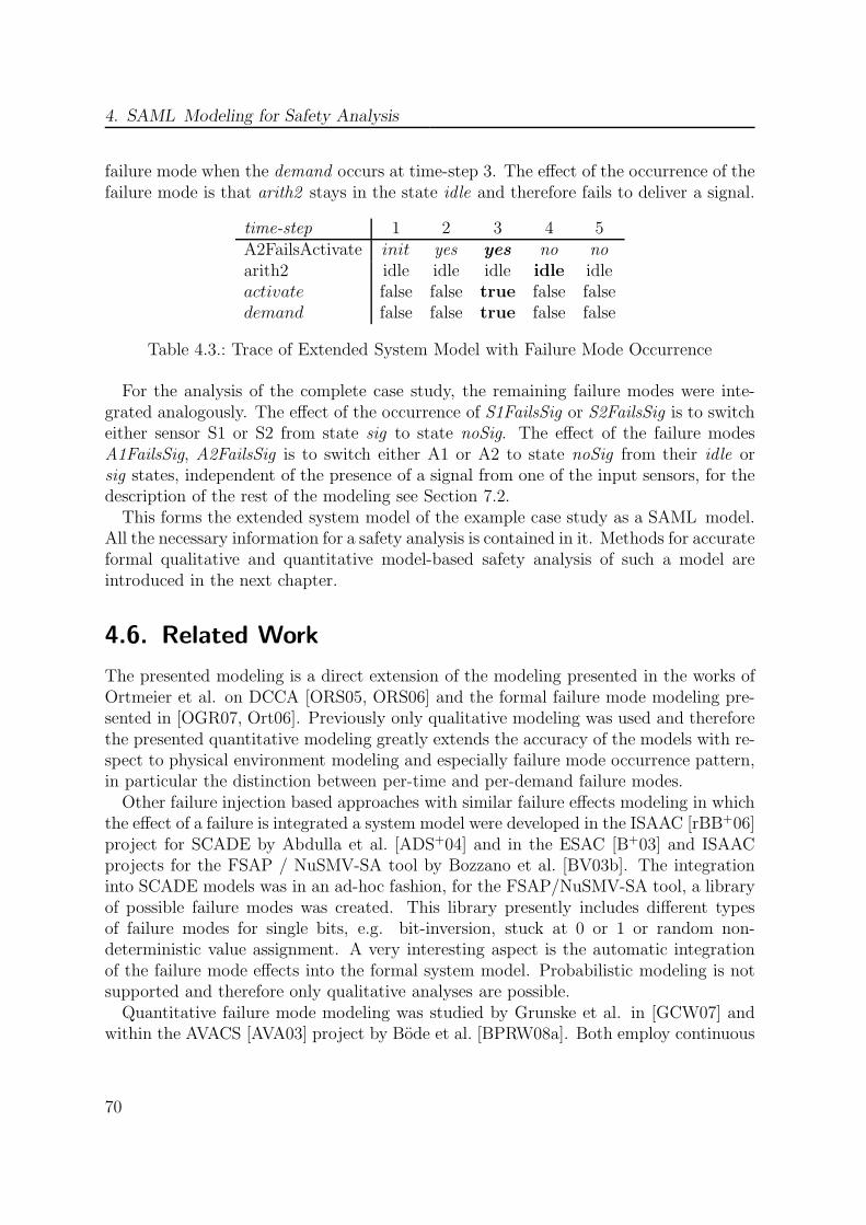
4. SAML Modeling for Safety Analysis
failure mode when the demand occurs at time-step 3. The effect of the occurrence of thefailure mode is that arith2 stays in the state idle and therefore fails to deliver a signal.
time-step 1 2 3 4 5A2FailsActivate init yes yes no noarith2 idle idle idle idle idleactivate false false true false falsedemand false false true false false
Table 4.3.: Trace of Extended System Model with Failure Mode Occurrence
For the analysis of the complete case study, the remaining failure modes were inte-grated analogously. The effect of the occurrence of S1FailsSig or S2FailsSig is to switcheither sensor S1 or S2 from state sig to state noSig. The effect of the failure modesA1FailsSig, A2FailsSig is to switch either A1 or A2 to state noSig from their idle orsig states, independent of the presence of a signal from one of the input sensors, for thedescription of the rest of the modeling see Section 7.2.This forms the extended system model of the example case study as a SAML model.
All the necessary information for a safety analysis is contained in it. Methods for accurateformal qualitative and quantitative model-based safety analysis of such a model areintroduced in the next chapter.
4.6. Related Work
The presented modeling is a direct extension of the modeling presented in the works ofOrtmeier et al. on DCCA [ORS05, ORS06] and the formal failure mode modeling pre-sented in [OGR07, Ort06]. Previously only qualitative modeling was used and thereforethe presented quantitative modeling greatly extends the accuracy of the models with re-spect to physical environment modeling and especially failure mode occurrence pattern,in particular the distinction between per-time and per-demand failure modes.Other failure injection based approaches with similar failure effects modeling in which
the effect of a failure is integrated a system model were developed in the ISAAC [rBB+06]project for SCADE by Abdulla et al. [ADS+04] and in the ESAC [B+03] and ISAACprojects for the FSAP / NuSMV-SA tool by Bozzano et al. [BV03b]. The integrationinto SCADE models was in an ad-hoc fashion, for the FSAP/NuSMV-SA tool, a libraryof possible failure modes was created. This library presently includes different typesof failure modes for single bits, e.g. bit-inversion, stuck at 0 or 1 or random non-deterministic value assignment. A very interesting aspect is the automatic integrationof the failure mode effects into the formal system model. Probabilistic modeling is notsupported and therefore only qualitative analyses are possible.Quantitative failure mode modeling was studied by Grunske et al. in [GCW07] and
within the AVACS [AVA03] project by Bode et al. [BPRW08a]. Both employ continuous
70

4.6. Related Work
failure mode modeling with failure rates which does not allow for per-demand failuremode modeling. The integration of the failure effects is similar to the methods pre-sented here and the conservative integration principle could also be extended to theseapproaches for failure mode modeling. Nevertheless in these approaches there is no ex-plicit failure occurrence pattern modeling. On the one hand, this reduces state spaceas there is no need for additional state variables modeling the occurrence. But on theother hand, this reduces the expressiveness of the modeling or at least increases thecomplexity of the models, as more has to be integrated into the system model itself.A very recent approach to formal safety analysis was developed in the COMPASS
project [BCK+09a] where a subset of the architecture analysis and design language(AADL) [SA04] and its error annex [SA06] is used. It allows for the specification offailure modes and is formalized in the SLIM language described by Bozzano et al.in [BCK+09b, BCK+10b]. This is a further development based on the FSAP/NuSMV-SA tool. It allows for the specification of hybrid systems with constant continuouslychanging variables and failure modes with a continuous time model. Analogously to theFSAP/NuSMV-SA tool, the integration of the failure modes into the formal system canbe done automatically. As only continuous modeling is provided, no per-demand fail-ure mode modeling is supported. Per-demand failure mode modeling is one part of theAADL error annex not supported by SLIM. The usage of the established modeling lan-guage AADL is very interesting. A formal semantics of AADL and its error annex whichallows for the integration of per-time and per-demand failure mode modeling would bea promising application of using SAML as an intermediate language.
Summary
This chapter introduced a modeling guideline to construct extended system models inSAML for formal model-based safety analysis. Extended system models consist of hard-ware, software and environment modeling. The environment model specifies the physicalbehavior of the system’s surroundings and the failure modes that are possible in the sys-tem. The existing formal failure modeling was extended with probabilistic failure modemodeling. The modeling of different types of probabilistic failure modes, namely per-time and per-demand was introduced and the conservative integration of the failuremodes was shown which provably retains the original behavior of the system after theintegration of the failure effects. The modeling approach was illustrated using a casestudy taken from the safety analysis literature.
71

5. Formal Safety Analysis
There are two ways to write error-free programs;only the third one works.
(Alan J. Perlis)
This chapter introduces methods which allow for formal model-based safety analysisof extended system models specified in SAML. Qualitative analyses allow for the com-putation of critical combinations of failure modes and deduction of temporal orderingsequences of these failure modes. Extensions of existing qualitative safety analysis meth-ods are developed which allow for analysis of self-healing systems. New methods candeduce dynamic fault trees (DFT) information directly from a SAML extended systemmodel.This chapter also introduces new, quantitative safety analysis methods which allow for
computation of the occurrence probability of a system hazard with much higher accuracythan previously possible. The methods use current state-of-the art probabilistic model-checking tools to compute hazard probabilities directly from SAML extended systemmodels.All analyses are formulated as temporal logic proof obligations which can be verified
automatically. The proof obligations are constructed in such a way that the resultingsafety analysis is guaranteed to be sound and complete. The application of the analysismethods is illustrated on the case study introduced in the previous chapter.Section 5.1 gives a motivation for the formal safety analysis techniques. Section 5.2
presents qualitative safety-analysis techniques which extend the existing qualitativesafety analysis methods. Section 5.3 presents a new quantitative model-based safetyanalysis method. Related work is discussed in Section 5.4.
73
5. Formal Safety Analysis
5.1. Motivation
From the safety engineer’s point of view the most important questions in the developmentof a safety critical system are:
• “What can cause a hazard?”
• “What is the probability that a hazard occurs?”
The model-based safety analysis methods presented in this chapter serve to answerthese questions correctly. If a formal system model is available, formalizing them as proofobligations can be very convenient, as model checking tools can compute the answersfully automatically.Nevertheless, the correct formalizing of these properties is not trivial. The main
considerations for the formalization are correctness and completeness of the analysis. Forsafety analysis, completeness refers to the fact that no cause of the hazard is forgotten.This means that each combination of failure modes is found which can cause the hazard.Correctness on the other hand means that for each combination of failure modes thatcan cause the hazard, there actually exists a run of the system on which it causes thehazard.A safety analysis technique should be both complete and correct. If it is correct,
it is never too optimistic and will never label an unsafe system as safe, which mightrender the system more dangerous than presumed. If the analysis is complete, then it isnot too pessimistic and will not label a potentially safe system as unsafe, which mightprevent its realization. So proving completeness and correctness of an analysis techniqueis important for the actual applications, especially if a system is to be certified. If theapplied analysis is not considered correct, a certification may not be granted.In addition to find failure mode combinations that can cause a hazard, it is also very
interesting to analyze temporal dependencies of the failure modes. This means that twofailure modes may only cause the hazard if they occur in a given sequence. If for exampletwo failure modes γ1, γ2 can only cause a hazard if γ1 appears before γ2, the system canbe made safer by the introduction of a warning or entering a safe mode if γ1 occurs.Even more beneficial is the extension to quantitative safety analysis methods which
compute the occurrence probability of a hazard. In traditional analysis techniques, thisis often conducted a-posteriori by a quantitative estimation based on the qualitativeanalysis results. New developments in the field of probabilistic model checking and theincrease of available computing resources now allow for the direct quantitative analysis ofthe extended system model itself. Such an approach gives much more precise and reliableresults, because all dependencies inherent in the system are automatically considered.Overall, the qualitative analysis methods give a “yes or no” answer whereas quantita-
tive analysis methods provide a more differentiating and precise answer. Nevertheless,both kinds of analysis methods are necessary. Firstly because qualitative analysis are
74
5.2. Qualitative Model-Based Safety Analysis
much more efficient and should therefore be used were adequate. Secondly, for someaspects the naıve reasoning that probability zero means impossible is wrong.In general for a model-based safety analysis one will (i) built an extended system
model (as described in the previous chapter) (ii) analyze the qualitative properties ofthe system (potentially using the qualitative results to improve the system) and (iii)analyze the quantitative properties of the system.
5.2. Qualitative Model-Based Safety Analysis
Qualitative safety analysis techniques are of possibilistic nature. They compute whetherand how failure modes can cause a hazard in the worst case. These analyses are typi-cally the first which are conducted on an extended system model. One example is thedeductive cause-consequence analysis (DCCA). In this dissertation it forms the basisfor further qualitative analysis and is also the starting point of the quantitative safetyanalysis methods presented in this chapter.
5.2.1. Deductive Cause Consequence Analysis
DCCA is an approach to deduce information about critical failure mode combinationsfrom an extended system model. It forms the basis for the formal model-based safetyanalysis of SAML models. It computes whether a subset of the set of all failure modesis critical with respect to a hazard. Critical here means that the combined occurrenceof the failure modes can actually cause the hazard. The result of a DCCA is a set ofall critical combinations of failure modes. This information can be used to implementrisk-reducing measures. If from every such critical combination at least one failure modecan be prevented, then the occurrence of the hazard is impossible1. DCCA has beenintroduced by Ortmeier et al. in [ORS05] and has been successfully applied to severalcase studies [ORS06, ORS05, GOR08]. In the following, the notion of a SAML modelM or extended system model M+ is used in the formal specifications, instead of τMDP ,e.g. κ(M+) actually refers to the embedded Kripke structure of the corresponding MDPof M+. From the context the meaning is always clear. The definitions (28)-(29) and thefollowing description are adapted from [ORS05].
Definition 28. DCCA / Minimal Critical SetFor an extended system modelM+ and a set of failure modes ∆, a subset of component
failures Γ ⊆ ∆ is called critical wrt. a system hazard H if
κ(M+), s0 |= E [ΓUH ], where Γ :=∧
δi∈∆\Γ
¬δi
Γ is called minimal critical if is has on proper critical subset.
1This is often called the “minimal cut set theorem” whose name is derived from FTA.
75
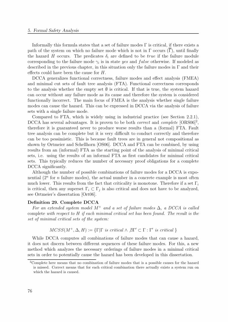
5. Formal Safety Analysis
Informally this formula states that a set of failure modes Γ is critical, if there exists apath of the system on which no failure mode which is not in Γ occurs (Γ), until finallythe hazard H occurs. The predicates δi are defined to be true if the failure modulecorresponding to the failure mode γi is in state yes and false otherwise. If modeled asdescribed in the previous chapter, in this situation only the failure modes in Γ and theireffects could have been the cause for H .DCCA generalizes functional correctness, failure modes and effect analysis (FMEA)
and minimal cut sets of fault tree analysis (FTA). Functional correctness correspondsto the analysis whether the empty set ∅ is critical. If that is true, the system hazardcan occur without any failure mode as its cause and therefore the system is consideredfunctionally incorrect. The main focus of FMEA is the analysis whether single failuremodes can cause the hazard. This can be expressed in DCCA via the analysis of failuresets with a single failure mode.Compared to FTA, which is widely using in industrial practice (see Section 2.2.1),
DCCA has several advantages. It is proven to be both correct and complete [ORS06]2,therefore it is guaranteed never to produce worse results than a (formal) FTA. Faulttree analysis can be complete but it is very difficult to conduct correctly and thereforecan be too pessimistic. This is because fault trees are in general not compositional asshown by Ortmeier and Schellhorn [OS06]. DCCA and FTA can be combined, by usingresults from an (informal) FTA as the starting point of the analysis of minimal criticalsets, i.e. using the results of an informal FTA as first candidates for minimal criticalsets. This typically reduces the number of necessary proof obligations for a completeDCCA significantly.Although the number of possible combinations of failure modes for a DCCA is expo-
nential (2n for n failure modes), the actual number in a concrete example is most oftenmuch lower. This results from the fact that criticality is monotone. Therefore if a set Γi
is critical, then any superset Γi ⊂ Γj is also critical and does not have to be analyzed,see Ortmeier’s dissertation [Ort06].
Definition 29. Complete DCCAFor an extended system model M+ and a set of failure modes ∆, a DCCA is called
complete with respect to H if each minimal critical set has been found. The result is theset of minimal critical sets of the system:
MCSS(M+,∆, H) := {Γ|Γ is critical ∧ 6 ∃Γ′ ⊂ Γ : Γ′ is critical }
While DCCA computes all combinations of failure modes that can cause a hazard,it does not discern between different sequences of these failure modes. For this, a newmethod which analyzes the necessary orderings of failure modes in a minimal criticalsets in order to potentially cause the hazard has been developed in this dissertation.
2Complete here means that no combination of failure modes that is a possible causes for the hazardis missed. Correct means that for each critical combination there actually exists a system run onwhich the hazard is caused.
76
5.2. Qualitative Model-Based Safety Analysis
5.2.2. Ordered Minimal Critical Sets
Failure modes that are causes for hazards can occur at different times on a systemtrace. If failure modes are in the same minimal critical set, then their appearance on atrace is considered critical, regardless of the sequence in which they occur. The resultsof a DCCA can be augmented by analyzing whether there exits a necessary temporalordering for the failure modes to be critical.
Failure Mode Ordering Relation
If a critical combination of failure modes for a system hazard is established, i.e. aminimal critical set is found by conducting a DCCA, then a partial order relation onthe failure modes can be defined. This relation captures the temporal ordering betweentwo failure modes in a minimal critical set3.
Definition 30. Before Order / Strict Before OrderFor an extended system model M+, a set of failure modes ∆, a predicate logic hazard
H, and a minimal critical set Γ ⊆ ∆, two failures modes γ1, γ2 ∈ Γ are in
• before order: γ1 �Γ γ2, if on all paths π of κ(M+) on which the failures in Γwere the cause for the hazard H, the first occurrence of the failure mode γ1 is notafter the first occurrence of the failure mode γ2
• strict before order: γ1 ≺Γ γ2, if on all paths π of κ(M+) on which the failuresin Γ were the cause for the hazard H, the failure mode γ2 does appear after thefailure mode γ1
If such an ordering exists, i.e. the relations are not empty, concentrating the risk-reducing measures on γ1 can be very beneficial. Alternatively, watchdogs can be usedto detect the occurrence of γ1 and if possible the system can enter a degraded “safemode”, in which no more safety-critical functions are executed. Based on these tworelations an additional relation for temporal ordering can be defined which describes thesimultaneous occurrence of two failure modes:
Definition 31. Simultaneous OrderFor an extended system model M+, a set of failure modes ∆, a predicate logic hazard
H and a minimal critical set Γ ⊆ ∆, two failure modes γ1, γ2 ∈ Γ are in simultaneousorder γ1 ∼Γ γ2, if on all paths π of κ(M+) on which the failures in Γ were the causefor the hazard H, the first occurrence of the failure mode γ1 is at the same time as thefirst occurrence of the failure mode γ2
∼Γ:= {(γi, γj)|γi �Γ γj ∧ γj �Γ γi} (5.1)
3This is not dependent on DCCA, but can also be employed to minimal cut sets of a fault tree analysis.
77
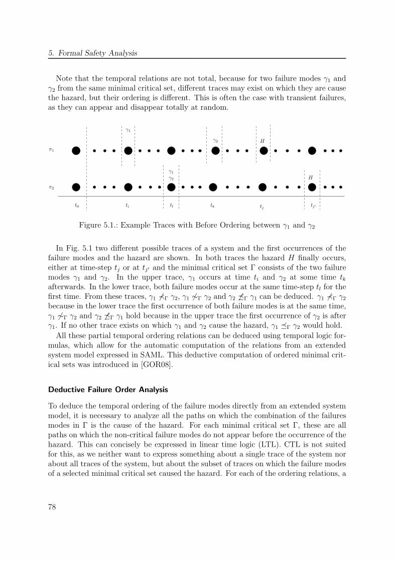
5. Formal Safety Analysis
Note that the temporal relations are not total, because for two failure modes γ1 andγ2 from the same minimal critical set, different traces may exist on which they are causethe hazard, but their ordering is different. This is often the case with transient failures,as they can appear and disappear totally at random.
tj′
γ1
t0 ti
γ1γ2
tj
Hγ2
tktl
H
π1
π2
Figure 5.1.: Example Traces with Before Ordering between γ1 and γ2
In Fig. 5.1 two different possible traces of a system and the first occurrences of thefailure modes and the hazard are shown. In both traces the hazard H finally occurs,either at time-step tj or at tj′ and the minimal critical set Γ consists of the two failuremodes γ1 and γ2. In the upper trace, γ1 occurs at time ti and γ2 at some time tkafterwards. In the lower trace, both failure modes occur at the same time-step tl for thefirst time. From these traces, γ1 6≺Γ γ2, γ1 6∼Γ γ2 and γ2 6�Γ γ1 can be deduced. γ1 6≺Γ γ2because in the lower trace the first occurrence of both failure modes is at the same time,γ1 6∼Γ γ2 and γ2 6�Γ γ1 hold because in the upper trace the first occurrence of γ2 is afterγ1. If no other trace exists on which γ1 and γ2 cause the hazard, γ1 �Γ γ2 would hold.
All these partial temporal ordering relations can be deduced using temporal logic for-mulas, which allow for the automatic computation of the relations from an extendedsystem model expressed in SAML. This deductive computation of ordered minimal crit-ical sets was introduced in [GOR08].
Deductive Failure Order Analysis
To deduce the temporal ordering of the failure modes directly from an extended systemmodel, it is necessary to analyze all the paths on which the combination of the failuresmodes in Γ is the cause of the hazard. For each minimal critical set Γ, these are allpaths on which the non-critical failure modes do not appear before the occurrence of thehazard. This can concisely be expressed in linear time logic (LTL). CTL is not suitedfor this, as we neither want to express something about a single trace of the system norabout all traces of the system, but about the subset of traces on which the failure modesof a selected minimal critical set caused the hazard. For each of the ordering relations, a
78

5.2. Qualitative Model-Based Safety Analysis
LTL formula is specified which computes whether the specified temporal ordering existsfor two failure modes of a minimal critical set.
Lemma 4. Deductive Before Ordering / Strict Before OrderingFor an extended system model M+, a set of failure modes ∆, a predicate logic hazard
H, a minimal critical set Γ and two failure modes γ1, γ2 ∈ Γ:
γ1 �Γ γ2 ⇔
κ(M+), π |= (ΓUH) → [(¬H ∧ ¬γ1 ∧ ¬γ2)
U(γ1 ∧ ((¬H ∧ ¬γ2)
U((γ2 ∧ ¬H) ∧ FH)))] (5.2)
γ1 ≺Γ γ2 ⇔
κ(M+), π |= (ΓUH) → [(¬H ∧ ¬γ1 ∧ ¬γ2)
U((γ1 ∧ ¬γ2 ∧ ¬H)∧
X((¬H ∧ ¬γ2)
U((γ2 ∧ ¬H) ∧ FH)))] (5.3)
proof see p. 170
The left part of the implications (ΓUH) describes those paths of the extended systemmodel on which the failure modes in Γ are the cause of the hazard (i.e. no failure modein ∆ \ Γ appears before H). The right part of the implication describes the relationof the failure modes on the path. For the before ordering it is assured that the firstoccurrence of γ2 is not after the first occurrence of γ1 (Eq. (5.2)). For the strict beforerelation, the temporal next (X) operator describes the situation that at least one timestep passed after the occurrence of γ1 before the first occurrence of γ2 (Eq. (5.3)).The relation ∼Γ can be checked either if for two failure modes γ1 �Γ γ2∧γ2 �Γ γ1 holds
or by checking the proof obligation in Eq. (5.4). In this proof obligation it is assuredthat the very first occurrence of both failure modes under consideration happens at thesame time and before the first occurrence of the hazard.
Lemma 5. Deductive Simultaneous OrderFor an extended system model M+, a set of failure modes ∆, a predicate logic hazard
H,a minimal critical set Γ and two failure modes γ1, γ2 ∈ Γ
γ1 ∼Γ γ2 ⇔
κ(M+), π |= (ΓUH) → [(¬H ∧ ¬γ1 ∧ ¬γ2)
U((γ1 ∧ γ2 ∧ ¬H) ∧ FH)] (5.4)
79
5. Formal Safety Analysis
proof see p. 171
All the described proof obligations are formulated for two failure modes. This meansthe temporal relation between two failure modes can be computed at a time. If more thantwo failures are included in a minimal critical set, then the relations must be computed
for all pairs of failures, i.e.
(
n
2
)
combinations for n failures. All these combinations
can easily be generated automatically from a given minimal critical set of failures modes.
Application of DCCA and Ordering Analysis
To illustrate a qualitative analysis using DCCA and the deductive ordering analysis, thecase study presented in the previous chapter is used. The six possible failure modes inthis case study are sensor signal omitting (S1FailsSig, S2FailsSig), malfunction of thearithmetic units (A1FailsSig, A2FailsSig), failure of the watchdog monitor (Monitor-Fails) which results in either unnecessary switching of arithmetic processing units ormissing a necessary switch and the failure of the activation of the backup arithmeticunit (A2FailsActivate). Using DCCA to analyze the case study presented in Section 4.2with the hazard “no output produced” results in the following minimal critical sets:
• Γ1 := {A1FailsSig}
• Γ2 := {A2FailsSig,MonitorFails}
• Γ3 := {MonitorFails,A2ActivateFails}
• Γ4 := {MonitorFails,S2FailsSig}
• Γ5 := {S1FailsSig,S2FailsSig}
The deductive ordering analysis of these five minimal critical sets shows that Monitor-Fails ≺Γ3 A2ActivateFails holds. Therefore the failure modes in the set {MonitorFails,A2ActivateFails} can only cause the system hazard if the monitor fails before the activa-tion of A2 fails. The critical situation arises when the monitor misdetects a malfunctionof A1, sends the activation signal but A2 does not get properly activated.The set Γ2 is critical when the monitor misdetects a malfunction of A1, the activation
of A2 succeeds, but then A2 fails. A similar situation occurs if S2 fails after the activationof A2 (Γ4). Here A2 does not receive an input signal from its only signal source S2. Theset Γ5 is critical because if both input sensors fail, then no more output signal can beproduced. These three sets do not exhibit any temporal ordering.The surprising result is the fact that Γ1 contains only A1FailsSig as a single point
of failure. As the system is built with A2 as a hot spare unit, this should not happen.Luckily, verification tools provide counterexamples for violated proof obligations whichcan be further analyzed to identify the flaw. A closer analysis of this situation reveals
80

5.2. Qualitative Model-Based Safety Analysis
that when A1 fails, the system needs a short amount of time to activate A2. In thistime, no output signal is produced and therefore A1FailsSig is considered a single pointof failure.
Nevertheless omitting the signal in this situation is only temporary and the systemgets operational again. This can be seen in the state sequence shown in Table 5.1. Herethe A1 unit fails to deliver a signal at causing the temporary hazard. This is observedby the monitoring unit which activates A2. When A2 starts delivering a signal, thetemporary malfunctioning is resolved.
time-step 1 2 3 4 5 6A1FailsSig no yes no no no noarith1 sig sig noSig noSig noSig noSigarith2 idle idle idle idle sig sigMonitor normal normal normal degraded off offH false false true true false false
Table 5.1.: Temporary Hazard Occurrence
Such an effect is not directly detectable with DCCA as the hazard is a Boolean pred-icate. One solution to this problem is to introduce an observer module which signalsthe hazard after a certain time passes. In this way some time-dependent hazards canbe expressed as Boolean predicates. This approach will be used for the quantitativeanalysis in Section 5.3.
But for qualitative safety analysis, on the other hand, a much more general and elegantapproach to cope with this problem is also possible. It can cope with more general self-healing systems which can recover from a temporary hazardous state. In order to analyzesuch systems correctly, a new variant of DCCA was developed in this dissertation thatcan cope directly with such situations.
5.2.3. Adaptive DCCA
To address the increasing complexity of modern systems, new paradigms of the de-velopment of system are developed which allow the system to decide certain aspectsautonomously. Prominent examples of these paradigms are IBM’s Autonomic Comput-ing Initiative proposed by Kephart and Chess [KC03] and Organic Computing proposedby Muller-Schloer et al. [MS04, MSvW04].
A very important subclass of these systems which could be very beneficial for safety-critical system are self-healing systems. These can recover autonomously from a tem-porary system hazard. This will most often be realized by the introduction of a certainamount of redundancy in the system. The drawback of the autonomy is that it is muchharder to give guarantees of the behavior of self-healing systems. Nevertheless, this is
81

5. Formal Safety Analysis
essential for using such systems in safety-critical applications. This dissertation presentsa new method for safety analysis and verification of such systems.
As shown in the example case study, DCCA cannot directly be applied to a self-healingsystem, as the hazard occurrence may only be temporary. If this is not reflected, a safetyanalysis would be too pessimistic, as a recovery after the occurrence of the hazard ispossible. As long as enough redundancy is available, a self-healing system can get backto its functional mode again or at least enter a degraded “safe mode”. Only a permanentoccurrence of the system hazard is considered critical. This fact is reflected in adaptiveDCCA (aDCCA) which was first introduced in [GOR06b] from where the definition (32),the following description and Lemma 6 are adapted.
Definition 32. aDCCA / Minimal Adaptive-Critical Set for Adaptive DCCA
For a system M+ and a set of failure modes ∆ a subset of component failures Γ ⊆ ∆is called adaptive-critical for a system hazard for a hazard H if
κ(M+), s0 |= E [Γ U (EG ( H ∧ Γ))] where Γ :=∧
δ∈(∆\Γ)
¬ δ
Γ a minimal adaptive-critical set if Γ is adaptive-critical and no proper subset of Γ isadaptive-critical.
The aDCCA proof obligation in Def. 32 states that a set of failure modes Γ is adaptive-critical if there exists a trace such that only these failure modes can lead to permanentsystem failure. The permanent occurrence of the hazard is expressed as EG (H ∧ Γ)which means that a continuation exists on which H holds in all states. The last part inthe formula (∧Γ) is necessary to assure the failures modes of Γ are the reason for thepermanent system hazard and no other failure mode occurs on the path continuation.
Just like with DCCA, the adaptive-criticality property of a set of failures is alsomonotonic for the notion of adaptive-critical sets. This means: ∀ Γ1,Γ2 ⊆ ∆ : Γ1 ⊆Γ2 ⇒ (Γ1 is adaptive-critical set ⇒ Γ2 is adaptive-critical set). A complete aDCCAand the resulting set of minimal adaptive-critical sets aMCSS(M+,∆, H) are definedanalogously to Def. 29.
Lemma 6. aDCCA Completeness
For a complete aDCCA of an extended system model M+, a set of failure modes ∆and a hazard H the following formula holds:
κ(M+), s0 |= A ((∧
Γ∈aMCSS(M+,∆,H)
¬∧
γj∈Γ
F γj) → ¬FGH)
proof see p. 172
82

5.2. Qualitative Model-Based Safety Analysis
For the formulation of the completeness lemma, CTL* logic is used. Fortunately theCTL subset – for which model-checking is much more efficient – is sufficient to computethe minimal adaptive-critical sets. The formula of Lemma (6) states, that on all (A )those traces on which from each minimal adaptive-critical set the occurrence of at leastone failure mode can be prevented (¬
∧
γj∈ΓF γj), the hazard can always be repaired by
the system again (¬FGH). In other words: the hazard can only become permanent ifall failure modes of at least one minimal adaptive-critical set occur. This means thataDCCA is complete and no cause for the hazard is omitted. The correctness of aDCCAcan also be guaranteed. For each minimal adaptive-critical set, the proof obligation inDef. 6 can compute a witness run of the system on which the combination of failuremodes causes the hazard4.The relation of aDCCA to DCCA is shown in Lemma (7). It states that every set
of failures that is considered adaptive-critical with aDCCA is also considered criticalwith DCCA. The other direction of the implication does not hold. As a counterexampleconsider a system where the hazard H can occur but is always repaired after k > 0 time-steps and is then absent for at least one time-step. Such a system never fails permanentlyand therefore is not considered adaptive-critical. Note that this also means that there isno necessary subset inclusion relation between the minimal critical sets and the minimaladaptive-critical sets. In the example above the occurrence of the temporary hazardwould be considered the cause of a minimal critical set, but there would be no minimaladaptive-critical superset of it.
Lemma 7. DCCA Implication for aDCCALet M+ be an extended system model, ∆ be a finite set of failure modes, Γ ⊆ ∆, and
M be the embedded Kripke structure of κ(M+) then
κ(M+), s0 |= E [ΓUEG (H ∧ Γ)] ⇒ κ(M+), s0 |= E [ΓUH ]
proof see p. 173
Just as in DCCA, the adaptive variant computes the critical combinations of failuremodes without considering any temporal ordering. Analogous to the deductive orderinganalysis of traditional systems, it is possible to specify proof obligations to compute theordering relations for a self-healing system.
Adaptive Deductive Ordering Analysis
The ordering relation of minimal adaptive-critical sets of a self-healing system can bededuced from a SAML model analogously to non-self-healing systems. For non-self-healing systems, all traces on which only the failure modes of a minimal adaptive-critical set appear before the hazard are of interest. For self-healing systems, the traces
4Most often this will be computed by specifying the negation of the proof obligation and using amodel-checker to compute a counterexample. A counterexample to the negation is then equivalentto a witness of the original proof obligation.
83

5. Formal Safety Analysis
to consider are those on which the non-critical failure modes do not appear at all andthe hazard finally becomes permanent.This situation is formalized as (ΓU(G (H ∧ Γ)). This is the precondition for each of
the proof obligations in the Lemmas (8) and (9). For a minimal adaptive-critical set Γ,this precondition describes all those traces on which the hazard H eventually becomespermanent and all failure modes that are not in Γ do not occur at all.
Lemma 8. Adaptive Deductive Before Ordering / Strict Before OrderingFor an extended system model M+, a set of failure modes ∆, a predicate logic hazard
H, a minimal adaptive-critical set Γ and two failure modes γ1, γ2 ∈ Γ,
γ1 �Γ γ2 ⇔
κ(M+), π |= (ΓU(G (H ∧ Γ)) → [(¬γ1 ∧ ¬γ2)
U(γ1 ∧ ((¬γ2)
U(γ2 ∧ (FGH)))] (5.5)
γ1 ≺Γ γ2 ⇔
κ(M+), π |= (ΓU(G (H ∧ Γ))) → [(¬γ1 ∧ ¬γ2)
U((γ1 ∧ ¬γ2)∧
X((¬γ2)
U(γ2 ∧ (FGH))))] (5.6)
proof see p. 173
Analogously to the deductive ordering analysis for non-self-healing systems, the proofobligations assure that the first occurrence of γ1 is not after the first occurrence of γ2 forthe before ordering, respectively the first occurrence of γ2 is at least one time step afterthe first occurrence of γ1. The difference here is the omission of ¬H , as the eventualpermanent occurrence of the hazard (FGH) is of interest.
Lemma 9. Adaptive Deductive Simultaneous OrderFor an extended system model M+, a set of failure modes ∆, a predicate logic hazard
H, a minimal adaptive-critical set Γ and two failure modes γ1, γ2 ∈ Γ
γ1 ∼Γ γ2 ⇔
κ(M+), π |= (ΓU(G (H ∧ Γ)) → [(¬γ1 ∧ ¬γ2)
U((γ1 ∧ γ2) ∧ (FGH))] (5.7)
proof see p. 174
The combination of aDCCA and adaptive deductive ordering analysis can easily beapplied to the example case study, by checking the respective proof obligations.
84

5.2. Qualitative Model-Based Safety Analysis
Application of adaptive DCCA and Deductive Ordering Relation Analysis
In contrast to the first analysis with DCCA, where the recovery from the temporaryhazard after the failure of A1 was not anticipated, no more single point of failure isidentified with this more accurate analysis. For the analysis of combinations of twofailure modes, 15 combinations had to be checked with aDCCA. This lead to the following8 minimal adaptive-critical sets:
• Γ1 := {A1FailsSig,A2FailsSig}
• Γ2 := {A1FailsSig,MonitorFails}
• Γ3 := {A1FailsSig,A2FailsActivate}
• Γ4 := {A1FailsSig,S2FailsSig}
• Γ5 := {A2FailsSig,MonitorFails}
• Γ6 := {MonitorFails,A2FailsActivate}
• Γ7 := {MonitorFails,S2FailsSig}
• Γ8 := {S1FailsSig,S2FailsSig}
The minimal adaptive-critical sets Γ5,Γ6,Γ7,Γ8 are equivalent to the results of DCCA.For Γ6, the temporal relation MonitorFails≺Γ6A2FailsActivate holds. The differences ofDCCA and aDCCA are the first four minimal adaptive-critical sets which all includethe failure of A1, which was considered a single point of failure in the prior analysis.The first set Γ1 describes the situation that both arithmetic units fail. If this happens,
no more output signal can be produced. The critical combination in set Γ4 results fromthe situation where A1 fails, A2 gets activated, but S2 fails to deliver a signal. Neitherof these two minimal adaptive-critical sets exhibits a temporal ordering.The sets Γ2 and Γ3 describe two situations where A1 fails, but the system does not cor-
rectly enter its degraded mode. Either because the monitor fails to detect that A1 failed(Γ2) or because the activation of A2 fails (Γ3). The temporal ordering analysis of thesetwo sets reveals that bothMonitorFails�Γ2A1FailsSig and A1FailsSig≺Γ3A2FailsActivatehold. This means that the minimal adaptive-critical set Γ2 is only critical if the monitorfails before or at the same time as A1 fails. For Γ3 to be critical, the failure modeA1FailsSig must occur strictly before A2FailsActivate.In the case of Γ3 and Γ6 the failure mode which must appear after the first failure
mode is the per-demand failure mode A2FailsActivate. This is not surprising, as thedemand is triggered by the watchdog monitor which tries to activate A2. This demandcan only be triggered if either the monitor detects a malfunction of A1 or if the monitoritself fails with a misdetection. Therefore per-demand failure modes will often be in such
85

5. Formal Safety Analysis
a temporal relation. Nevertheless it is not mandatory, e.g. if not a single failure modeoccurrence is critical, but a sequence.Summarizing, a precise qualitative analysis of extended SAML system models is pos-
sible with the new qualitative analysis methods aDCCA for minimal adaptive-criticalsets and the deductive ordering analyses. These extend the range of systems which areanalyzable and allow for a further refinement of the analysis. This results in a moreprecise qualitative analysis of extended SAML system models than possible before. Foreach critical combination of failure modes, witness paths can be computed and analyzedthat show how the combination of the failure modes can cause the hazard. This informa-tion can be used to augment the systems by the integration of risk-reducing measures.Once this has been completed, quantitative analysis can be used to compute the overallprobability of the occurrence of a hazard.
5.3. Quantitative Model-Based Safety Analysis
After the possibilistic qualitative safety analysis and the potential introduction of risk-reducing measures, the next step is to apply a probabilistic, quantitative safety analysis.In many traditional safety analysis approaches, the occurrence probability of a systemhazard is computed a-posteriori on the results of a qualitative analysis. Starting fromthe occurrence probabilities of the single failure modes, the overall hazard probabilityis estimated. This is most often based on the “fault tree formula” shown in Eq. (5.8)which is used in FTA to estimate the probability for the minimal cut sets to causethe top-level event. But is also used for the minimal critical sets of DCCA or in theFSAP/NuSMV-SA tool by Bozzano and Villafiorita [BV03b].
P (H) ≤∑
Γ∈MCSS(M+,∆,H)
∏
γ∈Γ
P (γ) (5.8)
This estimation can be very coarse, it cannot even be guaranteed that the result ofthe sum on the right hand part is below 1! The reason for this is that only the resultsof a qualitative analysis of the formal system model are used. Therefore the estimationmust be very conservative. It is also assumed that all failure modes are stochasticallyindependent, which is very often not the case. For example, if there exists a temporalordering relation for some minimal critical sets. In addition, it is completely unclearhow per-time failure rates and per-demand failure probabilities can be combined in suchan approach.
5.3.1. Probabilistic DCCA
To overcome this problem, a new method was developed in this dissertation which ex-ploits the probabilistic information in an extended system model expressed in SAML. Itcomputes the overall occurrence probability of a hazard directly on the formal system
86
5.3. Quantitative Model-Based Safety Analysis
model. Analogous to the usage of CTL for DCCA and aDCCA, the probabilistic logicPCTL (see Section 3.4.2) is used for probabilistic DCCA (pDCCA) which was introducedin [GO10b].
Definition 33. Probabilistic DCCA (pDCCA)For an extended system model M+ and a hazard H, if
M+, s0 |= Pmax[trueUH ]>0 (5.9)
holds, then the computation of the probability
P (H) := Pmax=?[trueUH ] (5.10)
is called the probabilistic DCCA.
By using pDCCA, the problems outlined above are eliminated. The coarse estimationis replaced with an accurate computation of the occurrence probability. Assumptionsabout the stochastic independence are not necessary, as existing dependencies are auto-matically considered. This of course also includes the effect of possible temporal orderingrelations. All these influences on the overall hazard probability are implicitly and au-tomatically considered in the pDCCA formula and can be checked directly on a SAMLextended system model [GO10a].It is important to note that this analysis computes the overall hazard probability of all
minimal critical sets together. The probability that a single minimal critical set causesthe hazard cannot easily be calculated. The reason for this is that the PCTL analogonof the DCCA proof obligation, Pmax[ΓUH ]>0, does not formalize “maximal probabilityof traces on which only failure modes in Γ may cause H”. Traces can exist where thefailure modes of Γ cause the hazard, but other failure modes also appear, but withouthaving an effect. Any such trace would not be considered in this formula which thereforedoes not formalize this property. A correct formalization of this property would requirethe ability to reference the caused effect of a failure mode and should be formalized as:“maximal probability of traces on which only the failure effects of failure modes in Γmay cause H”. Unfortunately it is not yet clear whether it is possible to express thiswithout elaborate changes to the SAML system model.pDCCA in the form as shown in Def. 33 is well suited for non-reactive systems which
do not continue to run infinitely. A reactive system potentially runs infinitely long (atleast in an abstract view). This means that the system hazard will occur eventually.The reason for this is that semantics of PCTL is defined over infinite traces of a system.If a reactive system were analyzed with pDCCA as in Eq. (5.10), this would result inhazard probability of 1, as in general every combination of failure modes will eventuallyoccur on an infinite trace and therefore the hazard is inevitable. This does not offermore information than pure qualitative analysis, and is therefore not adequate for thequantitative analysis of reactive systems.
87

5. Formal Safety Analysis
5.3.2. Probabilistic DCCA for Reactive Systems
To overcome this problem and to make pDCCA feasible for the analysis of reactivesystems, the computation of the occurrence probability of the hazard is restricted tofinite traces. In particular a mission time of the safety-critical system is specified whichrepresents the considered time interval for the quantitative analysis.This mission time is defined as a multiple of the temporal resolution of the system.
Then the occurrence probability of the hazard can be computed using the bounded untilPCTL operator (see Eq. (3.5)). If Pmax[φU
≤kψ]>0 holds, then there exists, with non-zeroprobability, a bound j ≤ k, so that ψ becomes true after no more that j steps and φ istrue for all time steps i < j. Using this, the overall probability of the occurrence of thehazard of a reactive system can be computed with the bounded variant of pDCCA fora given mission time t = k ·∆t.
Definition 34. Bounded pDCCAFor an extended system model M+ and a hazard H, if
M+, s0 |= Pmax[trueU≤kH ]>0 (5.11)
holds, the computation of the probability
P (H) := Pmax=?[trueU≤kH ] (5.12)
is called the bounded pDCCA with mission time t = k ·∆t.
If the analyzed system is not a reactive system, the mission time is basically system-inherent and does not influence the outcome of the analysis5. In this case the constant kof the equation (5.12) can be set to∞ and the bounded until operator effectively becomesunbounded and it corresponds to a general pDCCA. As the probability of a boundeduntil operator is computed iteratively and the unbounded operator can be computeddirectly in one single step, it is advisable to use pDCCA if possible, to minimize thetime needed for the analysis.Specifying a “correct” mission time for a bounded pDCCA is not trivial. It is obvious
that a single step or too few steps in general may result in a zero hazard probability,which will often be unrealistic. The specification of too long mission times can renderthe analysis infeasible because of the required running time. The goal is to specify arealistic mission time that covers a representative time interval for the system. At theend of the next section first approaches to address these challenges are presented.
5.3.3. Adaptive pDCCA
Unfortunately, using pDCCA directly for adaptive systems is not as straightforward asit is for qualitative analysis. The PCTL analogon of the aDCCA formula would be
5After a given time, “nothing interesting” will happen in such systems, in particular no hazard occur-rence.
88
5.3. Quantitative Model-Based Safety Analysis
Pmax=?[trueUPmax[GH ]>0]. This cannot be used to compute the probability that thehazard eventually becomes permanent. The reason for this is that the CTL formulaEGφ is not equal to Pmax[Gφ]>0. An example for this has been shown in Fig. 3.7. Thesame holds for the bounded variant of the above formula Pmax=?[trueU
≤kPmax[GH ]>0].
A solution which can be used to handle this problem if the maximal time of thetemporary hazard is known, is to introduce an additional observer module. The statesof such a module then signal whether the hazard has occurred permanently or justtemporary and the permanent hazard occurrence can therefore be reduced to a Booleanpredicate. Most often this will be realized by counting the number of time-steps thehazard is present. If it is possible to decide whether the occurrence is permanent (e.g.the hazard was present longer than the maximal time to be only temporary), thena Boolean predicate (“Observer is in state X”) can be used to signal the permanenthazard occurrence. pDCCA (or bounded pDCCA for reactive systems) can then beused for quantitative analysis of such a system.
This additional observer module must of course not be allowed to change the probabil-ity of the resulting traces. This means that the observer must only contain deterministictransitions and no non-deterministic or probabilistic choices6. Then the parallel compo-sition with the other SAML modules does not change the probability of the resultingtraces.
Application of pDCCA
An observer module was added for the quantitative analysis of the example case study.The observer module was modeled as shown in Fig. 5.2. Its initial state init is left if thesystem is started. The successor states of init is state ok if either A1 or A2 produces asignal, or state “error1” if no valid signal is produced from either arithmetic unit. Thissituation is similar for the waiting states error1 and error2, there is a return to state okif a signal is produced or a state change to the next state if no such signal is available.If this happens in state error2, the successor is the state hazard. If the observer entersthis state, the system did not produce a signal for three time steps in a row which isconsidered as a permanent hazard.
The case study was analyzed for a running time of 10h. It is a reactive system,therefore bounded pDCCA was used. As described in the failure mode modeling in theprevious chapter, the temporal resolution was ∆t = 10ms. This translates to an analysistime of k = 3.600.000 steps for a mission time of 10h. The overall maximal probabilitythat the system fails to deliver an output signal within 10h of operational time (usingthe failure rates and probabilities as described in Section 4.5.2 is therefore:
Pmax=?[trueU≤3.600.000(observerSig = hazard)] = 9.1490 · 10−7 (5.13)
6This means all probabilistic choice must have probability 1
89

5. Formal Safety Analysis
Module observer / observerSig
init
1
1
1
1
1
1
1
signal
signal
¬started
ok
started ∧ ¬signal
started ∧ signal
error1 error2
hazard
true
¬signal
¬signal
¬signal
Figure 5.2.: Observer Automaton
Extrapolation of Results and Effects of Different Temporal Resolutions
The probability that the hazard occurs in the case study was computed for the missiontime of 10h. The time needed for a bounded pDCCA is directly dependent on thenumber of time-steps, as the algorithms used for the computation carry out k matrix-vector multiplications for k time-steps. This can lead to very long or even infeasiblerunning times for large case studies. Reducing the number of necessary multiplicationsfor the algorithm itself, e.g. by using a square and multiply approach, is not possible, asthis generally destroys the sparsity of the underlying models and significantly increasesthe memory requirements.Because of this, methods to reduce the analysis time without reducing the accuracy
(or only slightly reducing the accuracy) would be very beneficial. The most importantfactors that determine the number of steps k are the temporal resolution and the missiontime. This raises the question how different temporal resolutions affect the results andwhether the pDCCA results for a mission time t can be extrapolated to a longer timet′ > t without explicitly analyzing this mission time.Whether and how this is possible in general is still an open question. But the effect
of different temporal resolutions on the overall analysis result and the possibility toextrapolate from a shorter to a longer analysis interval can be analyzed experimentally.
Accuracy of the Failure Approximation The accuracy of the discrete approximationof the per-time failure rates with the geometric distribution has been discussed in Sec-tion 4.5.2. To analyze the effect of this accuracy on the overall hazard probability, twodifferent temporal resolutions, ∆t1 = 10ms and ∆t2 = 1s were considered. For thefailure rate 10−2 1
hof the failure mode S1FailsSig, the maximal and cumulative relative
90

5.3. Quantitative Model-Based Safety Analysis
error for t = 10h is shown in table 5.2.
∆t1 = 10ms ∆t2 = 1smaximal relative error 1.2710 · 10−8 4.4577 · 10−4
cumulative relative error 1.3889 · 10−6 0.048764
Table 5.2.: Relative Approximation Error for Failure Rates
This table shows that the order of magnitude of the approximation error is roughlythe same as the ratio of the lower to the higher temporal resolution, and that the higherresolution approximates slightly better than explainable only by the ratios. The twodifferent temporal resolutions were then used to analyze the system with pDCCA (afterall other model parameters were adjusted accordingly). The result for ∆t1 is shown inEq. (5.14), the result for ∆t2 is shown in Eq. (5.15).
Pmax=?[trueU≤3.600.000H ] ≈ 9.1490 · 10−7 (5.14)
Pmax=?[trueU≤36.000H ] ≈ 9.2707 · 10−7 (5.15)
From these results, one can conclude that the orders of magnitude of the approxi-mation errors for the failure rates does not necessarily influence the overall result in acomparable way. For a coarser first estimate, a lower temporal resolution can be ade-quate. This could be used to compare different variants of a system, possibly identifyingthe most promising variants and analyze those later with more accuracy.
Extrapolation of pDCCA Results For this experiment, the computed pDCCA of thecase study were used to determine the accuracy of an extrapolation of a mission time of10h (with ∆t = 10ms) from shorter mission times. The computed hazard probabilitiesup to 10h are shown in Fig. 5.3. The results were computed in 10s steps.Three different methods were used to extrapolate a longer mission time from the com-
puted results for t = 10s, 20s, 30s, 40s. A simple, rather obvious form of extrapolation isa directly proportional one. This means to use the quotient t′
t(the quotient of the longer
time interval to the analyzed interval) as a scaling factor to extrapolate the probabilities.This results in a linear approximation.As second approach a cubic approximation was chosen which is based on the numer-
ical derivations of the computed probabilities. The function graph of the computedprobabilities for every continuous cumulative probability distribution is monotone andchanges its curvature. Therefore a cubic extrapolation was used because it is the simplestapproach that can also change the curvature.The third approach was to use an exponential function of the form 1− b · e−ct and to
use optimization techniques to find the parameters b and c such that the approximationis best for the computed values wrt. the sum of squared deviances.
91
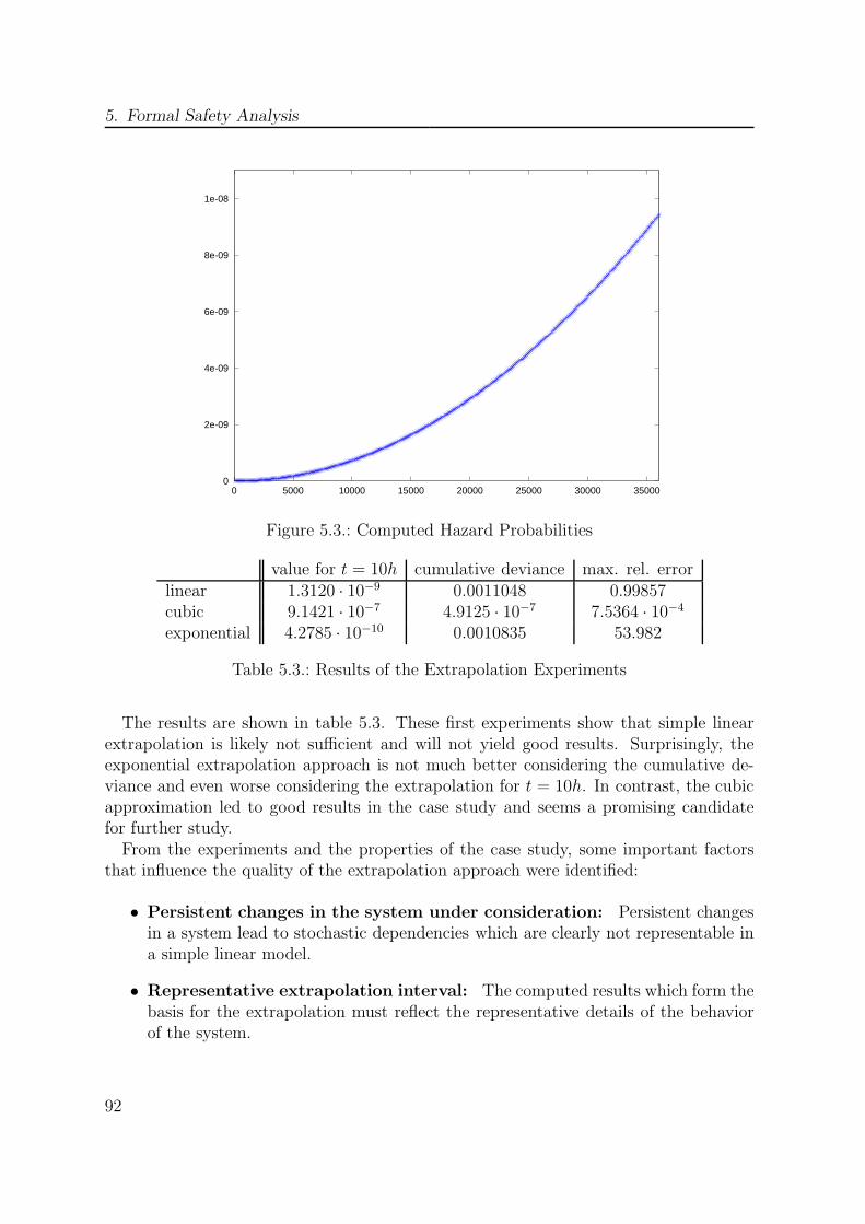
5. Formal Safety Analysis
0
2e-09
4e-09
6e-09
8e-09
1e-08
0 5000 10000 15000 20000 25000 30000 35000
Figure 5.3.: Computed Hazard Probabilities
value for t = 10h cumulative deviance max. rel. errorlinear 1.3120 · 10−9 0.0011048 0.99857cubic 9.1421 · 10−7 4.9125 · 10−7 7.5364 · 10−4
exponential 4.2785 · 10−10 0.0010835 53.982
Table 5.3.: Results of the Extrapolation Experiments
The results are shown in table 5.3. These first experiments show that simple linearextrapolation is likely not sufficient and will not yield good results. Surprisingly, theexponential extrapolation approach is not much better considering the cumulative de-viance and even worse considering the extrapolation for t = 10h. In contrast, the cubicapproximation led to good results in the case study and seems a promising candidatefor further study.From the experiments and the properties of the case study, some important factors
that influence the quality of the extrapolation approach were identified:
• Persistent changes in the system under consideration: Persistent changesin a system lead to stochastic dependencies which are clearly not representable ina simple linear model.
• Representative extrapolation interval: The computed results which form thebasis for the extrapolation must reflect the representative details of the behaviorof the system.
92

5.4. Related Work
Whether there are persistent changes in a system can be verified by checking whethera representative state after the starting phase of a system can always be reached again.If this is possible, then there is always a way to “reset” the system and an extrapolationof the probabilities is reasonable. Some ongoing research in this area is done by Seguinet al. [TIS11] for the new EPOCH probabilistic model-checker. Here strongly connectedcomponents in the MDP are exploited to increase the efficiency of probabilistic model-checking. Such components could correspond to “non-resettable” system states.The choice of a representative interval can be reduced to find a good coverage of
states. This means that the mission time must be chosen in such a way that within itscorresponding time steps, as many states as possible are reachable. One approach tocheck for a representative interval could be to use bounded model checking described byClarke et al. [CBRZ01] to check whether all states are reachable within k steps. Theinfluence of probabilistic choices on the overall result is reduced with the length of theconsidered path. As pDCCA is a reachability analysis, such an extrapolation could besuited to identify promising system variants. Such approaches will be studied further inthe ProMoSA project (see the outlook in Section 8.2).
5.4. Related Work
The failure injection methods as developed by Abdulla et al. for SCADE [ADS+04] andby Bozzano and Villafiorita for FSAP / NuSMV-SA [BV03b] also employ a qualitativeanalysis for critical failure modes. In general, first a safety property is specified andthen a combination of failure modes is integrated into the system. If the verification ofthe safety property fails, the failure mode combination is considered critical. Using thismethod, a fault tree consisting of three layers can be deduced from the formal system.The lowest layer is the conjunction of the critical combinations of failure modes, thesecond layer is the disjunction of each critical failure mode set and the highest layeris the system hazard. This will always lead to a complete FTA, but in contrast toDCCA and aDCCA, there is no proof of correctness of the analysis. The chosen safetyproperties do not require the failure modes to be the actual cause of the hazard, this isonly assumed implicitly.
Dynamic Fault Trees Analysis (DFT) [vM02] extends qualitative fault tree analysiswith several addition fault tree gates that also capture some dynamics of the system.Two of these are priority-AND (PAND) and simultaneous-AND (SAND) which corre-spond to the temporal ordering of two basic events. A very similar notion of ordering isemployed in an algebraic technique based on Papadopoulos’ and McDermid’s Hip-HOPSnotation [PM91], developed by Walker et al. [WP07, WBP07]. In this approach besidesPAND, a priority-OR (POR) relation is defined. The correlation of the different tem-poral ordering relations, temporal fault tree gates and the Hip-HOPS notation is shownin Table 5.4.
The computation of temporal ordering of failure modes in minimal critical sets can
93
5. Formal Safety Analysis
Failure Order Relation Temporal Fault Tree Gate Hip-HOPSφ1 �Γ φ2 (φ1SANDφ2)OR(φ1PANDφ2) φ1 < φ2 + φ1&φ2
φ1 ≺Γ φ2 φ1PANDφ2 φ1 < φ2
φ1 ∼Γ φ2 φ1SANDφ2 φ1&φ2
Table 5.4.: Temporal Ordering Notations
automatically construct dynamic fault trees with the temporal ordering gates PAND andSAND. For minimal (adaptive-)critical sets, failure modes in POR relation are consideredas single point of failures. Therefore no automatic deduction of a priority OR relation isspecified. A technique to deduce dynamic fault tree gates via a temporal failure modeordering from a formal system model is presented by Bozzano and Villafiorita in [BV03a]and integrated into the FSAP / NuSMV-SA tool by Bozzano et al. [BV03b]. In contrastto deductive ordering analysis, an additional state variable is introduced into the systemwhich signals the failure mode ordering. Therefore formally, each time a different systemis analyzed. This is in contrast to deductive temporal ordering analysis, where the sameextended system model is analyzed, but with different proof obligations. Nevertheless,for most systems the analysis results will be similar for both methods.
The quantitative assessment of hazard probabilities of failure modes with temporalordering dependencies has been approached in different ways. Many approaches derivestate space based systems from a dynamic fault tree which represent the temporal or-dering of the failure modes. The underlying models for analysis can be stochastic PetriNets which are used for example by Raiteri [CR05] or Bernardi and Donatelli [BD04].Another possibility to analyze dynamic fault trees is to use Markov Chain variants asdescribed by Boudali et al. [BCS07b, BCS07a]. These models are then analyzed ascontinuous time Markov Chains (CTMC). Very often these approaches also support ad-ditional dynamic fault tree gates like functional dependency (FDEP), sequence (SEQ)or warm spare (WSP). As with all CTMC analysis, the assumption is made that allprobabilities are exponentially distributed.
An interesting approach was developed by Merle et al. [MRLB10, MRLV10] and isdescribed in detail by Merle in his dissertation thesis [Mer10]. It uses algebraic tech-niques to deduce probabilities from a dynamic fault tree. This allows for using arbitraryprobability distributions and is therefore more flexible than approaches based on Markovmodels. In SAML as in most other safety analysis approaches based on probabilisticmodel-checking, arbitrary probability distributions can only be approximated with sev-eral exponential (respectively geometric) distributions. This will very likely increase thestate space of the underlying MDP and is therefore less practical for non-exponentiallydistributed failure mode probabilities.
Quantitative analysis of system models similar to the ones presented here is oftenconducted on the basis of CTMC models. Bozzano et al. developed the SLIM lan-guage [BCK+09b, BCK+10b], which formalizes a subset of the AADL error annex. SLIM
94
5.4. Related Work
models can include a failure model which is analyzed with the MRMC model checkerafter the non-probabilistic parts of the system are abstracted away with bisimulationtechniques. This approach is described by Katoen et al. in [KKZJ07] and uses theSigRef tool developed by Wimmer et al. [WHH+06]. This “Performability Analysis”restricts the analyzable models at the moment to non-hybrid models which do not usecontinuous variables.
Grunske et al. introduced probabilistic failure modes and effects analysis (pFMEA)in [GCW07]. This technique allows to deduce FMEA tables with probabilities and over-all system hazard probabilities from a formal system description which also expressesfunctional properties. This approach is very similar to failure injection and is not onlya state space representation of an existing dynamic fault tree. It is extended by Al-jazaar et al. [AFG+09, AKLFL10] to also extract counterexamples from a quantitativesystem description, namely those with the highest probability of occurrence. Comparedto qualitative SAML analysis, this is more computationally expensive. But if feasible, itdelivers more information how the dependability of a system can be increased. An inte-gration of the generation of probabilistic counterexamples would also be very beneficialfor safety analysis based on SAML.
Within the AVACS project [AVA03], an approach to find the failure mode combinationthat accounts for the biggest part of the overall hazard probability is presented byBode et al. [BPRW08a]. The approach is called “Importance Analysis of Minimal CutSets”. Here, failure modes are integrated into a functional system model analogous tofailure injection. For the analysis, a quotient system is constructed using bisimulationtechniques. In the quotient system all traces are eliminated on which failure modesappear which are not currently analyzed. This is accomplished using the SigRef tooldeveloped by Wimmer et al. [WHH+06]. It is then used to rank the critical combinationsof failure modes relative to another. The problem here is that the analyzed system isdifferent for each analysis, and therefore strict propositions about the probabilities arenot possible. A relative ranking of minimal critical sets would also be possible in SAML,by using the PCTL analogon of the DCCA formula [GO10b].
Summary
This chapter introduced new qualitative and quantitative model-based analysis methods.New qualitative methods are the deductive temporal ordering analysis, adaptive DCCAand adaptive deductive temporal ordering analysis. The ordering analyses allow for amore precise analysis of the temporal relations of critical failure modes. In contrast toother approaches these analysis rely only on different temporal logic proof obligationsand do not require changes to the system model itself. Adaptive DCCA allows forprovably complete and correct qualitative safety analysis of self-healing systems. Safetyanalysis of these systems was not possible before the development of aDCCA.
This chapter also presented the quantitative analysis method pDCCA. It allows a
95
5. Formal Safety Analysis
much more precise computation of the occurrence probability than previous a-posteriorimethods which rely on the quantitative analysis of the results of a prior qualitativeanalysis. In contrast to other model-based safety analysis methods, the combinationof per-time and per-demand failure modes is possible. First experiments on the effectsof different temporal resolutions and the possibility to extrapolate pDCCA results tolonger mission times were very promising. pDCCA and approaches based on theseextrapolations will further be used to quickly identify promising system variants in theDFG-funded ProMoSA project [OG10] were the probabilistic analysis results will beused as objective function for system optimization.
96
6. Transformation and Analysis of
SAML Models
A man’s got to know his limitations.
(Harry Callahan)
The previous chapters introduced SAML, its semantics and several model-based safetyanalysis methods. SAML is designed to be a tool-independent intermediate language.For concrete analysis, an extended system model of a safety-critical system must betransformed into the input specification language of an appropriate analysis tool. Thischapter presents exemplary transformations to translate SAML models for state of theart probabilistic and symbolic model-checkers.Section 6.1 motivates the usage of model-checking tools for the analysis and explains
how SAML benefits from the design as tool-independent modeling and intermediatelanguage. Section 6.2 very briefly describes some details of the implementation of thetransformations. The transformations necessary for the analysis of quantitative aspectsof a SAML model with a probabilistic analysis tool are described in 6.3. The requiredtransformation for a qualitative analysis tool is described in Section 6.4. Related workis discussed in Section 6.5.
97

6. Transformation and Analysis of SAML Models
6.1. Motivation
Several efficient model-checking tools have been developed for the analysis of formalsystem specifications. For a long time, most research was focused on the analysis ofqualitative properties of systems, specified in different qualitative logics. The currentstate of the art is the compact representation of Kripke structures as (ordered) binarydecision diagrams (BDD) and their analysis based on symbolic model-checking developedby Burch et al. [BCM+90].
For the analysis of labeled Markov chains, probabilistic model-checking has becomepractical in recent years. It is driven primarily by the massive increase of computingresources, the development of efficient numerical model-checking algorithms and thedevelopment of space-efficient representations of Markov models. While representationsbased on sparse matrices are very time-efficient, new approaches based on multi-terminalbinary decision diagrams (MTBDD) as described by de Alfaro et al. [dAKN+00] allow fora much more space-efficient representation of Markov models. This makes even very largestate spaces accessible for analysis, analogously to the BDD representation of symbolicmodel-checkers. In both cases giving a concise number of states for an analyzable systemis not possible in general, as this depends on many different system-specific factors.
The development of both qualitative and quantitative model-checkers is still an ac-tive research area. A lot of current research for probabilistic model-checking focuseson exploiting parallelism. Bernadat et al. focus on multi-core architectures [BBC+08],Bosnacki et al. [BES09] use the GPUs of modern graphic hardware to accelerate thenecessary numerical computations. Maisonneuve presents in her Master’s thesis [Mai09]approaches to optimize the MTBDD representation with heuristic variable reorderingwhich increases the range of analyzable models. Other methods are based on bisimula-tion techniques for more efficient analyses [KKZJ07, HWP+06, WHH+06]. To benefitfrom this ongoing research and the resulting improvements, in particular from the in-crease in analysis efficiency, SAML is designed as a tool-independent language that canbe transformed into the input specification of different analysis frameworks.
This can be achieved by using model transformations to transform SAML modelsinto model descriptions suitable for formal analysis with verification tools. An impor-tant aspect for this was to keep SAML as simple as possible, but at the same time beingexpressive enough for accurate modeling of extended system models for safety analy-sis. Using semantically founded transformations, it can be assured that the analyzedmodels are equivalent1. Therefore the analysis results of different verification tools are“compatible” with each other. This allows to choose the most appropriate analysis tooldepending on the character of the property but also on the efficiency of the availableverification tool. Obvious examples are the model-based safety analyses presented in thelast chapter. DCCA / aDCCA and deductive ordering analysis would be analyzed withqualitative verification tools and pDCCA with quantitative ones.
1For example the equivalency between the paths of the MDP and its embedded Kripke structure.
98
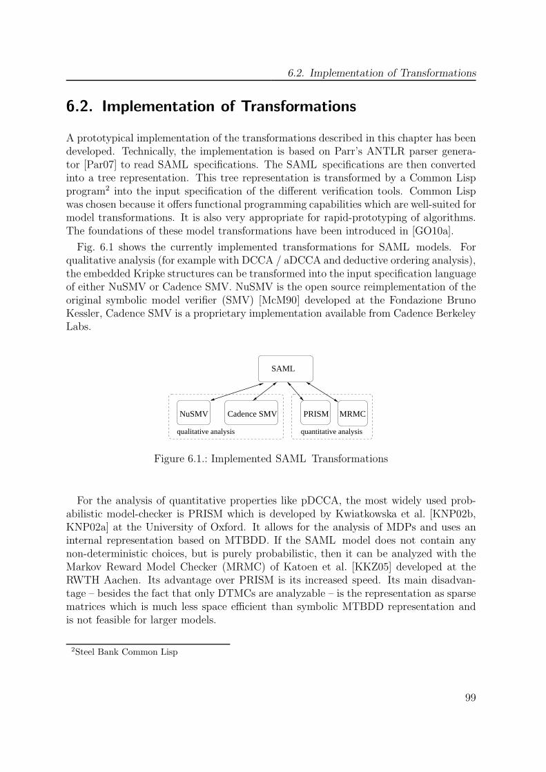
6.2. Implementation of Transformations
6.2. Implementation of Transformations
A prototypical implementation of the transformations described in this chapter has beendeveloped. Technically, the implementation is based on Parr’s ANTLR parser genera-tor [Par07] to read SAML specifications. The SAML specifications are then convertedinto a tree representation. This tree representation is transformed by a Common Lispprogram2 into the input specification of the different verification tools. Common Lispwas chosen because it offers functional programming capabilities which are well-suited formodel transformations. It is also very appropriate for rapid-prototyping of algorithms.The foundations of these model transformations have been introduced in [GO10a].
Fig. 6.1 shows the currently implemented transformations for SAML models. Forqualitative analysis (for example with DCCA / aDCCA and deductive ordering analysis),the embedded Kripke structures can be transformed into the input specification languageof either NuSMV or Cadence SMV. NuSMV is the open source reimplementation of theoriginal symbolic model verifier (SMV) [McM90] developed at the Fondazione BrunoKessler, Cadence SMV is a proprietary implementation available from Cadence BerkeleyLabs.
NuSMV Cadence SMV PRISM MRMC
quantitative analysisqualitative analysis
SAML
Figure 6.1.: Implemented SAML Transformations
For the analysis of quantitative properties like pDCCA, the most widely used prob-abilistic model-checker is PRISM which is developed by Kwiatkowska et al. [KNP02b,KNP02a] at the University of Oxford. It allows for the analysis of MDPs and uses aninternal representation based on MTBDD. If the SAML model does not contain anynon-deterministic choices, but is purely probabilistic, then it can be analyzed with theMarkov Reward Model Checker (MRMC) of Katoen et al. [KKZ05] developed at theRWTH Aachen. Its advantage over PRISM is its increased speed. Its main disadvan-tage – besides the fact that only DTMCs are analyzable – is the representation as sparsematrices which is much less space efficient than symbolic MTBDD representation andis not feasible for larger models.
2Steel Bank Common Lisp
99
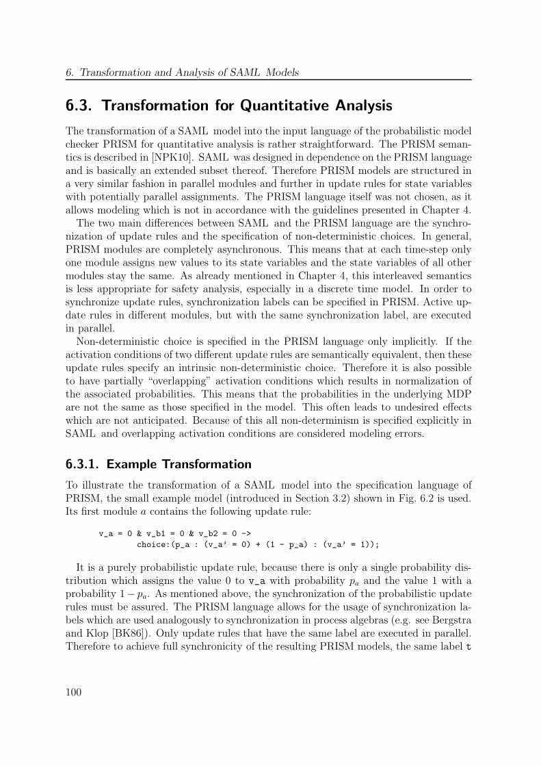
6. Transformation and Analysis of SAML Models
6.3. Transformation for Quantitative Analysis
The transformation of a SAML model into the input language of the probabilistic modelchecker PRISM for quantitative analysis is rather straightforward. The PRISM seman-tics is described in [NPK10]. SAML was designed in dependence on the PRISM languageand is basically an extended subset thereof. Therefore PRISM models are structured ina very similar fashion in parallel modules and further in update rules for state variableswith potentially parallel assignments. The PRISM language itself was not chosen, as itallows modeling which is not in accordance with the guidelines presented in Chapter 4.The two main differences between SAML and the PRISM language are the synchro-
nization of update rules and the specification of non-deterministic choices. In general,PRISM modules are completely asynchronous. This means that at each time-step onlyone module assigns new values to its state variables and the state variables of all othermodules stay the same. As already mentioned in Chapter 4, this interleaved semanticsis less appropriate for safety analysis, especially in a discrete time model. In order tosynchronize update rules, synchronization labels can be specified in PRISM. Active up-date rules in different modules, but with the same synchronization label, are executedin parallel.Non-deterministic choice is specified in the PRISM language only implicitly. If the
activation conditions of two different update rules are semantically equivalent, then theseupdate rules specify an intrinsic non-deterministic choice. Therefore it is also possibleto have partially “overlapping” activation conditions which results in normalization ofthe associated probabilities. This means that the probabilities in the underlying MDPare not the same as those specified in the model. This often leads to undesired effectswhich are not anticipated. Because of this all non-determinism is specified explicitly inSAML and overlapping activation conditions are considered modeling errors.
6.3.1. Example Transformation
To illustrate the transformation of a SAML model into the specification language ofPRISM, the small example model (introduced in Section 3.2) shown in Fig. 6.2 is used.Its first module a contains the following update rule:
v_a = 0 & v_b1 = 0 & v_b2 = 0 ->
choice:(p_a : (v_a’ = 0) + (1 - p_a) : (v_a’ = 1));
It is a purely probabilistic update rule, because there is only a single probability dis-tribution which assigns the value 0 to v_a with probability pa and the value 1 with aprobability 1− pa. As mentioned above, the synchronization of the probabilistic updaterules must be assured. The PRISM language allows for the usage of synchronization la-bels which are used analogously to synchronization in process algebras (e.g. see Bergstraand Klop [BK86]). Only update rules that have the same label are executed in parallel.Therefore to achieve full synchronicity of the resulting PRISM models, the same label t
100
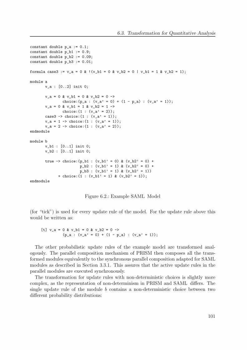
6.3. Transformation for Quantitative Analysis
constant double p_a := 0.1;
constant double p_b1 := 0.9;
constant double p_b2 := 0.09;
constant double p_b3 := 0.01;
formula case3 := v_a = 0 & !(v_b1 = 0 & v_b2 = 0 | v_b1 = 1 & v_b2 = 1);
module a
v_a : [0..2] init 0;
v_a = 0 & v_b1 = 0 & v_b2 = 0 ->
choice:(p_a : (v_a’ = 0) + (1 - p_a) : (v_a’ = 1));
v_a = 0 & v_b1 = 1 & v_b2 = 1 ->
choice:(1 : (v_a’ = 2));
case3 -> choice:(1 : (v_a’ = 1));
v_a = 1 -> choice:(1 : (v_a’ = 1));
v_a = 2 -> choice:(1 : (v_a’ = 2));
endmodule
module b
v_b1 : [0..1] init 0;
v_b2 : [0..1] init 0;
true -> choice:(p_b1 : (v_b1’ = 0) & (v_b2’ = 0) +
p_b2 : (v_b1’ = 1) & (v_b2’ = 0) +
p_b3 : (v_b1’ = 1) & (v_b2’ = 1))
+ choice:(1 : (v_b1’ = 1) & (v_b2’ = 1));
endmodule
Figure 6.2.: Example SAML Model
(for “tick”) is used for every update rule of the model. For the update rule above thiswould be written as:
[t] v_a = 0 & v_b1 = 0 & v_b2 = 0 ->
(p_a : (v_a’ = 0) + (1 - p_a) : (v_a’ = 1));
The other probabilistic update rules of the example model are transformed anal-ogously. The parallel composition mechanism of PRISM then composes all the trans-formed modules equivalently to the synchronous parallel composition adapted for SAMLmodules as described in Section 3.3.1. This assures that the active update rules in theparallel modules are executed synchronously.The transformation for update rules with non-deterministic choices is slightly more
complex, as the representation of non-determinism in PRISM and SAML differs. Thesingle update rule of the module b contains a non-deterministic choice between twodifferent probability distributions:
101
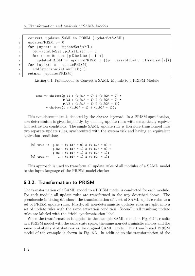
6. Transformation and Analysis of SAML Models
1 convert−updates−SAML−to−PRISM (updateSetSAML)2 updatesPRISM := ∅3 for ( update u : updateSetSAML)4 (φ , va r i ab l eSe t , pDi s tL i s t ) := u5 for ( i = 0 ; i < | pDi s tL i s t | ; i++)6 updatesPRISM := updatesPRISM ∪ {(φ , va r i ab l eSe t , pDi s tL i s t [ i ] ) }7 for ( update u : updatePRISM)8 addSynchronizat ionTick (u)9 return (updatesPRISM)
Listing 6.1: Pseudocode to Convert a SAML Module to a PRISM Module
true -> choice:(p_b1 : (v_b1’ = 0) & (v_b2’ = 0) +
p_b2 : (v_b1’ = 1) & (v_b2’ = 0) +
p_b3 : (v_b1’ = 1) & (v_b2’ = 1))
+ choice:(1 : (v_b1’ = 1) & (v_b2’ = 1));
This non-determinism is denoted by the choice keyword. In a PRISM specification,non-determinism is given implicitly, by defining update rules with semantically equiva-lent activation conditions. The single SAML update rule is therefore transformed intotwo separate update rules, synchronized with the system tick and having an equivalentactivation condition:
[t] true -> p_b1 : (v_b1’ = 0) & (v_b2’ = 0) +
p_b2 : (v_b1’ = 1) & (v_b2’ = 0) +
p_b3 : (v_b1’ = 1) & (v_b2’ = 1);
[t] true -> 1 : (v_b1’ = 1) & (v_b2’ = 1);
This approach is used to transform all update rules of all modules of a SAML modelto the input language of the PRISM model-checker.
6.3.2. Transformation to PRISM
The transformation of a SAML model to a PRISM model is conducted for each module.For each module all update rules are transformed in the way described above. Thepseudocode in listing 6.1 shows the transformation of a set of SAML update rules to aset of PRISM update rules. Firstly, all non-deterministic updates rules are split into aset of update rules with the same activation condition. Secondly, all resulting updaterules are labeled with the “tick” synchronization label.When the transformation is applied to the example SAML model in Fig. 6.2 it results
in a PRISM model with the same state space, the same non-deterministic choices and thesame probability distributions as the original SAML model. The transformed PRISMmodel of the example is shown in Fig. 6.3. In addition to the transformation of the
102

6.3. Transformation for Quantitative Analysis
mdp
const double p_a = 0.1;
const double p_b1 = 0.9;
const double p_b2 = 0.09;
const double p_b3 = 0.01;
formula case3 = v_a = 0 & !(v_b1 = 0 & v_b2 = 0 | v_b1 = 1 & v_b2 = 1);
module a
v_a : [0..2] init 0;
[t] v_a = 0 & v_b1 = 0 & v_b2 = 0 -> p_a : (v_a’ = 0) + (1 - p_a) : (v_a’ = 1);
[t] v_a = 0 & v_b1 = 1 & v_b2 = 1 -> 1 : (v_a’ = 2);
[t] case3 -> 1 : (v_a’ = 1);
[t] v_a = 1 -> 1 : (v_a’ = 1);
[t] v_a = 2 -> 1 : (v_a’ = 2);
endmodule
module b
v_b1 : [0..1] init 0;
v_b2 : [0..1] init 0;
[t] true -> p_b1 : (v_b1’ = 0) & (v_b2’ = 0) +
p_b2 : (v_b1’ = 1) & (v_b2’ = 0) +
p_b3 : (v_b1’ = 1) & (v_b2’ = 1);
[t] true -> 1 : (v_b1’ = 1) & (v_b2’ = 1) ;
endmodule
Figure 6.3.: Transformed PRISM Model
update rules, the constant definitions and the Boolean variables are also adjusted to thePRISM syntax.
An additional detail of PRISM models is the explicit specification whether it is a MDPor a DTMC. This is noted in the first line with the keywords dtmc or mdp. Althoughany DTMC is just a special case of MDP, the analysis of DTMCs can be much moretime efficient. In addition, if a SAML model can be expressed as a DTMC, it can alsobe analyzed with the MRMC model-checker. Its current version cannot analyze MDPsbut experiments have shown that it is much more time efficient than PRISM for theanalysis of feasible models. Its input language is very simple and requires the explicitsparse transition matrix and the labeling of each state. The easiest way to create thisis to use the export function of PRISM which constructs the state space of the DTMCand then exports the state space and the labeling function in the format appropriate forMRMC.
103

6. Transformation and Analysis of SAML Models
6.4. Transformation for Qualitative Analysis
For qualitative safety analysis, a SAML model is converted into a description of itsembedded Kripke structure. One possible approach would be to convert the MDP of aSAML model directly into a Kripke structure on the semantic level. This means that itstransition relation would be encoded directly and not using a notion of parallel moduleswith state variables. Another possible approach is the transformation on the syntacticallevel, i.e. transforming SAML modules into similar parallel module representation ofthe embedded Kripke structure.
The disadvantage of a transformation on the semantic level compared to a syntactictransformation is that it would require the construction of the whole state space. Thisis very inefficient as this has to be done for both the transformation and also for thelater analysis. An important advantage of the transformation on the syntactical level isthat it allows for a much better traceability of the model artifacts. This is very helpfulin safety analysis, in particular for the interpretation of counterexamples. Thereforethe choice was made to transform SAML models on the syntactical level for qualitativesafety analysis.
Perhaps the most prominent example of a model-checker for Kripke structures is thesymbolic model verifier (SMV) [McM90, BCM+90] which can verify both CTL and LTLproperty specifications. Several variants of SMV exist, the most current and accessibleone is the open-source reimplementation NuSMV by Cimatti et al. [CCG+02]. It isavailable for many platforms in binary and source code form and is under ongoingdevelopment. Because of its availability and good performance it is used here as analysistool for qualitative properties of SAML models. The described transformation for otherSMV variants like Cadence SMV differs only in minor details and is not explained indetail here3.
Analogously to SAML, NuSMV models are also structured as parallel modules whichcan contain one or more state variables. An obvious difference of NuSMV to SAMLis of course the absence of probabilistic update rules as NuSMV models can only benon-deterministic. A minor difference is that a complete model is constructed from theparallel composition of a set of single modules which must explicitly be imported in adistinguished main module. This means that every NuSMV model has to include a mainmodule and that a SAML module named main must be renamed for the transformation.
A more subtle difference of SAML and the NuSMV specification language makesthe transformation challenging. SAML allows for parallel assignments of new valuesto variables in a single update rule. This can be very convenient in a probabilisticenvironment, where not only the fact is of interest that a parallel assignment is possible,but also how probable a specific one is. As to my current knowledge, such parallelassignments are not directly expressible in the specification language of NuSMV (or of
3The transformation to Cadence SMV is also implemented, the syntax of the input language is slightlydifferent, the method of the transformation and the structure of the transformed models is the same.
104
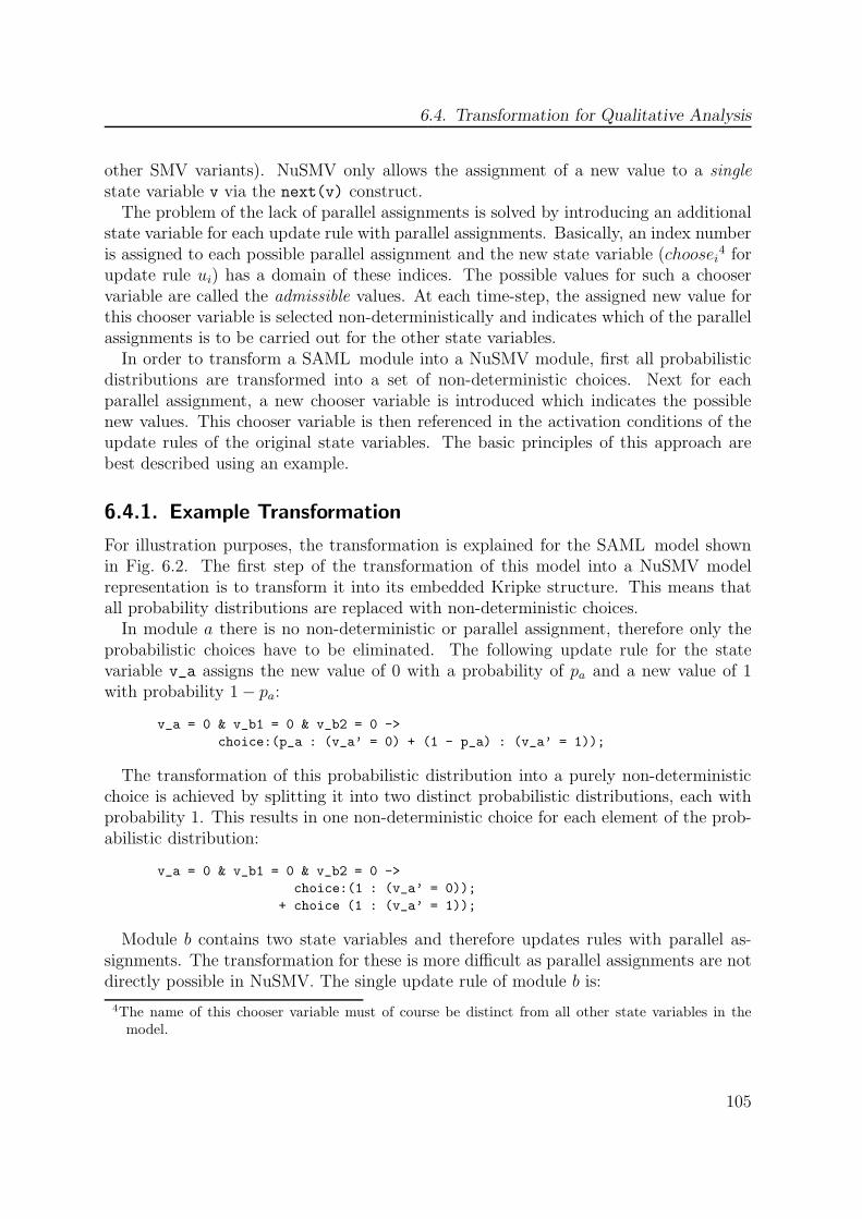
6.4. Transformation for Qualitative Analysis
other SMV variants). NuSMV only allows the assignment of a new value to a singlestate variable v via the next(v) construct.The problem of the lack of parallel assignments is solved by introducing an additional
state variable for each update rule with parallel assignments. Basically, an index numberis assigned to each possible parallel assignment and the new state variable (choosei
4 forupdate rule ui) has a domain of these indices. The possible values for such a chooservariable are called the admissible values. At each time-step, the assigned new value forthis chooser variable is selected non-deterministically and indicates which of the parallelassignments is to be carried out for the other state variables.In order to transform a SAML module into a NuSMV module, first all probabilistic
distributions are transformed into a set of non-deterministic choices. Next for eachparallel assignment, a new chooser variable is introduced which indicates the possiblenew values. This chooser variable is then referenced in the activation conditions of theupdate rules of the original state variables. The basic principles of this approach arebest described using an example.
6.4.1. Example Transformation
For illustration purposes, the transformation is explained for the SAML model shownin Fig. 6.2. The first step of the transformation of this model into a NuSMV modelrepresentation is to transform it into its embedded Kripke structure. This means thatall probability distributions are replaced with non-deterministic choices.In module a there is no non-deterministic or parallel assignment, therefore only the
probabilistic choices have to be eliminated. The following update rule for the statevariable v_a assigns the new value of 0 with a probability of pa and a new value of 1with probability 1− pa:
v_a = 0 & v_b1 = 0 & v_b2 = 0 ->
choice:(p_a : (v_a’ = 0) + (1 - p_a) : (v_a’ = 1));
The transformation of this probabilistic distribution into a purely non-deterministicchoice is achieved by splitting it into two distinct probabilistic distributions, each withprobability 1. This results in one non-deterministic choice for each element of the prob-abilistic distribution:
v_a = 0 & v_b1 = 0 & v_b2 = 0 ->
choice:(1 : (v_a’ = 0));
+ choice (1 : (v_a’ = 1));
Module b contains two state variables and therefore updates rules with parallel as-signments. The transformation for these is more difficult as parallel assignments are notdirectly possible in NuSMV. The single update rule of module b is:
4The name of this chooser variable must of course be distinct from all other state variables in themodel.
105
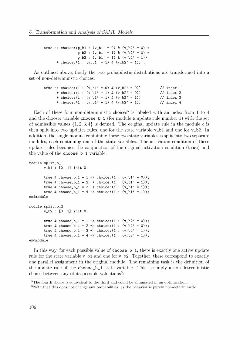
6. Transformation and Analysis of SAML Models
true -> choice:(p_b1 : (v_b1’ = 0) & (v_b2’ = 0) +
p_b2 : (v_b1’ = 1) & (v_b2’ = 0) +
p_b3 : (v_b1’ = 1) & (v_b2’ = 1))
+ choice:(1 : (v_b1’ = 1) & (v_b2’ = 1)) ;
As outlined above, firstly the two probabilistic distributions are transformed into aset of non-deterministic choices:
true -> choice:(1 : (v_b1’ = 0) & (v_b2’ = 0)) // index 1
+ choice:(1 : (v_b1’ = 1) & (v_b2’ = 0)) // index 2
+ choice:(1 : (v_b1’ = 1) & (v_b2’ = 1)) // index 3
+ choice:(1 : (v_b1’ = 1) & (v_b2’ = 1)); // index 4
Each of these four non-deterministic choices5 is labeled with an index from 1 to 4and the chooser variable choose_b_1 (for module b update rule number 1) with the setof admissible values {1, 2, 3, 4} is defined. The original update rule in the module b isthen split into two updates rules, one for the state variable v_b1 and one for v_b2. Inaddition, the single module containing these two state variables is split into two separatemodules, each containing one of the state variables. The activation condition of theseupdate rules becomes the conjunction of the original activation condition (true) andthe value of the choose_b_1 variable:
module split_b_1
v_b1 : [0..1] init 0;
true & choose_b_1 = 1 -> choice:(1 : (v_b1’ = 0));
true & choose_b_1 = 2 -> choice:(1 : (v_b1’ = 1));
true & choose_b_1 = 3 -> choice:(1 : (v_b1’ = 1));
true & choose_b_1 = 4 -> choice:(1 : (v_b1’ = 1));
endmodule
module split_b_2
v_b2 : [0..1] init 0;
true & choose_b_1 = 1 -> choice:(1 : (v_b2’ = 0));
true & choose_b_1 = 2 -> choice:(1 : (v_b2’ = 0));
true & choose_b_1 = 3 -> choice:(1 : (v_b2’ = 1));
true & choose_b_1 = 4 -> choice:(1 : (v_b2’ = 1));
endmodule
In this way, for each possible value of choose_b_1, there is exactly one active updaterule for the state variable v_b1 and one for v_b2. Together, these correspond to exactlyone parallel assignment in the original module. The remaining task is the definition ofthe update rule of the choose_b_1 state variable. This is simply a non-deterministicchoice between any of its possible valuations6:
5The fourth choice is equivalent to the third and could be eliminated in an optimization.6Note that this does not change any probabilities, as the behavior is purely non-deterministic.
106
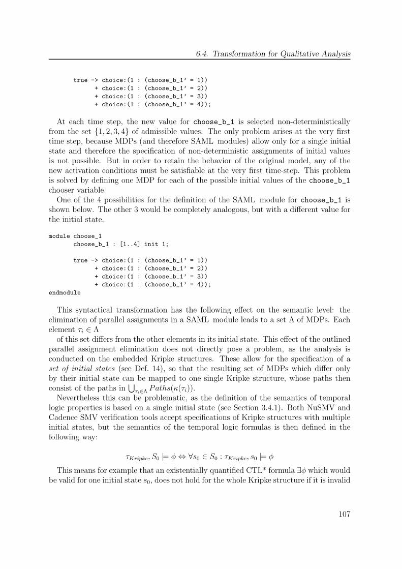
6.4. Transformation for Qualitative Analysis
true -> choice:(1 : (choose_b_1’ = 1))
+ choice:(1 : (choose_b_1’ = 2))
+ choice:(1 : (choose_b_1’ = 3))
+ choice:(1 : (choose_b_1’ = 4));
At each time step, the new value for choose_b_1 is selected non-deterministicallyfrom the set {1, 2, 3, 4} of admissible values. The only problem arises at the very firsttime step, because MDPs (and therefore SAML modules) allow only for a single initialstate and therefore the specification of non-deterministic assignments of initial valuesis not possible. But in order to retain the behavior of the original model, any of thenew activation conditions must be satisfiable at the very first time-step. This problemis solved by defining one MDP for each of the possible initial values of the choose_b_1
chooser variable.One of the 4 possibilities for the definition of the SAML module for choose_b_1 is
shown below. The other 3 would be completely analogous, but with a different value forthe initial state.
module choose_1
choose_b_1 : [1..4] init 1;
true -> choice:(1 : (choose_b_1’ = 1))
+ choice:(1 : (choose_b_1’ = 2))
+ choice:(1 : (choose_b_1’ = 3))
+ choice:(1 : (choose_b_1’ = 4));
endmodule
This syntactical transformation has the following effect on the semantic level: theelimination of parallel assignments in a SAML module leads to a set Λ of MDPs. Eachelement τi ∈ Λof this set differs from the other elements in its initial state. This effect of the outlined
parallel assignment elimination does not directly pose a problem, as the analysis isconducted on the embedded Kripke structures. These allow for the specification of aset of initial states (see Def. 14), so that the resulting set of MDPs which differ onlyby their initial state can be mapped to one single Kripke structure, whose paths thenconsist of the paths in
⋃
τi∈ΛPaths(κ(τi)).
Nevertheless this can be problematic, as the definition of the semantics of temporallogic properties is based on a single initial state (see Section 3.4.1). Both NuSMV andCadence SMV verification tools accept specifications of Kripke structures with multipleinitial states, but the semantics of the temporal logic formulas is then defined in thefollowing way:
τKripke, S0 |= φ⇔ ∀s0 ∈ S0 : τKripke, s0 |= φ
This means for example that an existentially quantified CTL* formula ∃φ which wouldbe valid for one initial state s0, does not hold for the whole Kripke structure if it is invalid
107
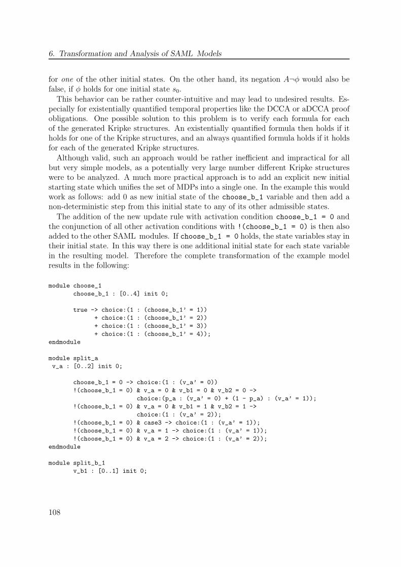
6. Transformation and Analysis of SAML Models
for one of the other initial states. On the other hand, its negation A¬φ would also befalse, if φ holds for one initial state s0.
This behavior can be rather counter-intuitive and may lead to undesired results. Es-pecially for existentially quantified temporal properties like the DCCA or aDCCA proofobligations. One possible solution to this problem is to verify each formula for eachof the generated Kripke structures. An existentially quantified formula then holds if itholds for one of the Kripke structures, and an always quantified formula holds if it holdsfor each of the generated Kripke structures.Although valid, such an approach would be rather inefficient and impractical for all
but very simple models, as a potentially very large number different Kripke structureswere to be analyzed. A much more practical approach is to add an explicit new initialstarting state which unifies the set of MDPs into a single one. In the example this wouldwork as follows: add 0 as new initial state of the choose_b_1 variable and then add anon-deterministic step from this initial state to any of its other admissible states.
The addition of the new update rule with activation condition choose_b_1 = 0 andthe conjunction of all other activation conditions with !(choose_b_1 = 0) is then alsoadded to the other SAML modules. If choose_b_1 = 0 holds, the state variables stay intheir initial state. In this way there is one additional initial state for each state variablein the resulting model. Therefore the complete transformation of the example modelresults in the following:
module choose_1
choose_b_1 : [0..4] init 0;
true -> choice:(1 : (choose_b_1’ = 1))
+ choice:(1 : (choose_b_1’ = 2))
+ choice:(1 : (choose_b_1’ = 3))
+ choice:(1 : (choose_b_1’ = 4));
endmodule
module split_a
v_a : [0..2] init 0;
choose_b_1 = 0 -> choice:(1 : (v_a’ = 0))
!(choose_b_1 = 0) & v_a = 0 & v_b1 = 0 & v_b2 = 0 ->
choice:(p_a : (v_a’ = 0) + (1 - p_a) : (v_a’ = 1));
!(choose_b_1 = 0) & v_a = 0 & v_b1 = 1 & v_b2 = 1 ->
choice:(1 : (v_a’ = 2));
!(choose_b_1 = 0) & case3 -> choice:(1 : (v_a’ = 1));
!(choose_b_1 = 0) & v_a = 1 -> choice:(1 : (v_a’ = 1));
!(choose_b_1 = 0) & v_a = 2 -> choice:(1 : (v_a’ = 2));
endmodule
module split_b_1
v_b1 : [0..1] init 0;
108

6.4. Transformation for Qualitative Analysis
choose_b_1 = 0 -> choice:(1 : (v_b1’ = 0));
!(choose_b_1 = 0) & true & choose_b_1 = 1 -> choice:(1 : (v_b1’ = 0));
!(choose_b_1 = 0) & true & choose_b_1 = 2 -> choice:(1 : (v_b1’ = 1));
!(choose_b_1 = 0) & true & choose_b_1 = 3 -> choice:(1 : (v_b1’ = 1));
!(choose_b_1 = 0) & true & choose_b_1 = 4 -> choice:(1 : (v_b1’ = 1));
endmodule
module split_b_2
v_b2 : [0..1] init 0;
choose_b_1 = 0 -> choice:(1 : (v_b2’ = 0));
!(choose_b_1 = 0) & true & choose_b_1 = 1 -> choice:(1 : (v_b2’ = 0));
!(choose_b_1 = 0) & true & choose_b_1 = 2 -> choice:(1 : (v_b2’ = 0));
!(choose_b_1 = 0) & true & choose_b_1 = 3 -> choice:(1 : (v_b2’ = 1));
!(choose_b_1 = 0) & true & choose_b_1 = 4 -> choice:(1 : (v_b2’ = 1));
endmodule
As all of the safety analyses presented in Chapter 5 are reachability analyses, this isa valid approach for SAML extended system models. The soundness of the outlinedtransformation is shown in the next section.
6.4.2. Formal Transformation
The general transformation of a SAML model for qualitative analysis works as follows:
1. Eliminate the probabilistic distributions
2. Eliminate the parallel assignments
3. Assemble the resulting set of models to a single one
To show the soundness of the outlined transformation of a SAML model some addi-tional definitions are necessary. To formalize the mapping of a SAML update rule to aset of update rules of solely non-deterministic choices without parallel assignments, anupdate tuple is defined as in Def. 35.
Definition 35. Update TupleAn update tuple (φ, V,Θ) consists of
• a Boolean activation condition φ
• a set of variables V
• a set Θ of probabilistic choices θ where each θ is a set of pairs of the form (p, Expr)where p is a probability and Expr is a set of pairs of state variables v ∈ V andexpressions that define their new values.
109
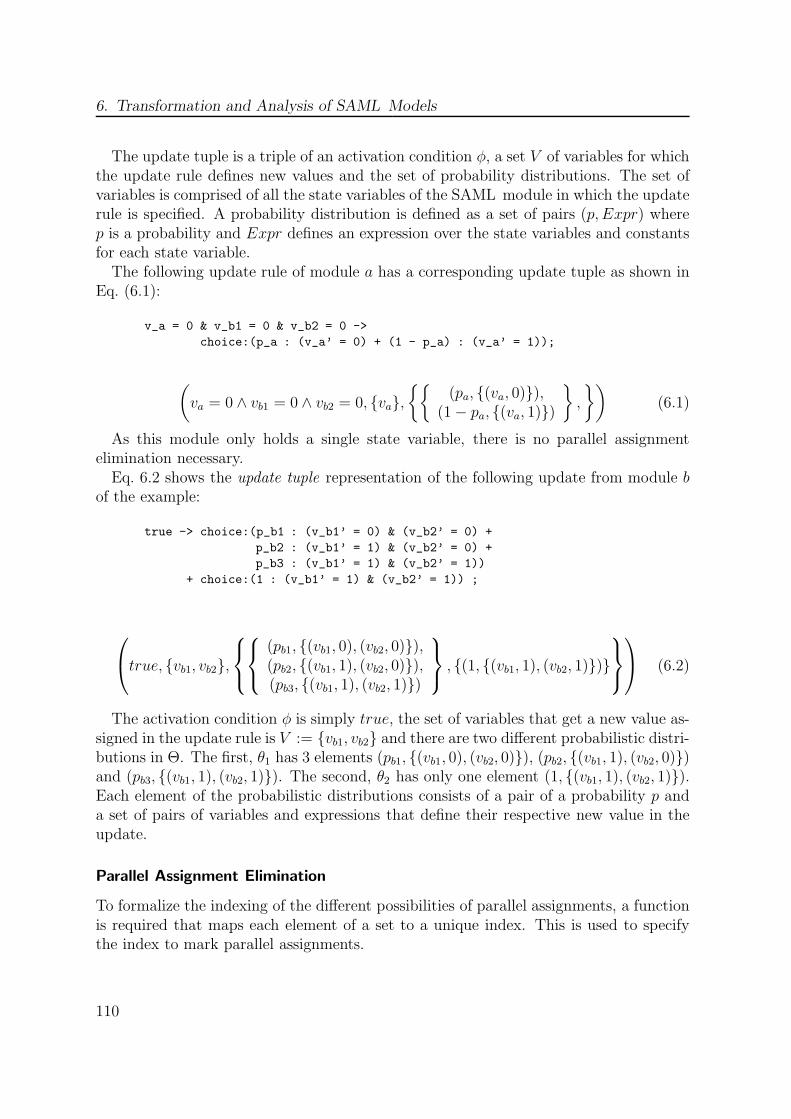
6. Transformation and Analysis of SAML Models
The update tuple is a triple of an activation condition φ, a set V of variables for whichthe update rule defines new values and the set of probability distributions. The set ofvariables is comprised of all the state variables of the SAML module in which the updaterule is specified. A probability distribution is defined as a set of pairs (p, Expr) wherep is a probability and Expr defines an expression over the state variables and constantsfor each state variable.The following update rule of module a has a corresponding update tuple as shown in
Eq. (6.1):
v_a = 0 & v_b1 = 0 & v_b2 = 0 ->
choice:(p_a : (v_a’ = 0) + (1 - p_a) : (v_a’ = 1));
(
va = 0 ∧ vb1 = 0 ∧ vb2 = 0, {va},
{{
(pa, {(va, 0)}),(1− pa, {(va, 1)})
}
,
})
(6.1)
As this module only holds a single state variable, there is no parallel assignmentelimination necessary.Eq. 6.2 shows the update tuple representation of the following update from module b
of the example:
true -> choice:(p_b1 : (v_b1’ = 0) & (v_b2’ = 0) +
p_b2 : (v_b1’ = 1) & (v_b2’ = 0) +
p_b3 : (v_b1’ = 1) & (v_b2’ = 1))
+ choice:(1 : (v_b1’ = 1) & (v_b2’ = 1)) ;
true, {vb1, vb2},
(pb1, {(vb1, 0), (vb2, 0)}),(pb2, {(vb1, 1), (vb2, 0)}),(pb3, {(vb1, 1), (vb2, 1)})
, {(1, {(vb1, 1), (vb2, 1)})}
(6.2)
The activation condition φ is simply true, the set of variables that get a new value as-signed in the update rule is V := {vb1, vb2} and there are two different probabilistic distri-butions in Θ. The first, θ1 has 3 elements (pb1, {(vb1, 0), (vb2, 0)}), (pb2, {(vb1, 1), (vb2, 0)})and (pb3, {(vb1, 1), (vb2, 1)}). The second, θ2 has only one element (1, {(vb1, 1), (vb2, 1)}).Each element of the probabilistic distributions consists of a pair of a probability p anda set of pairs of variables and expressions that define their respective new value in theupdate.
Parallel Assignment Elimination
To formalize the indexing of the different possibilities of parallel assignments, a functionis required that maps each element of a set to a unique index. This is used to specifythe index to mark parallel assignments.
110
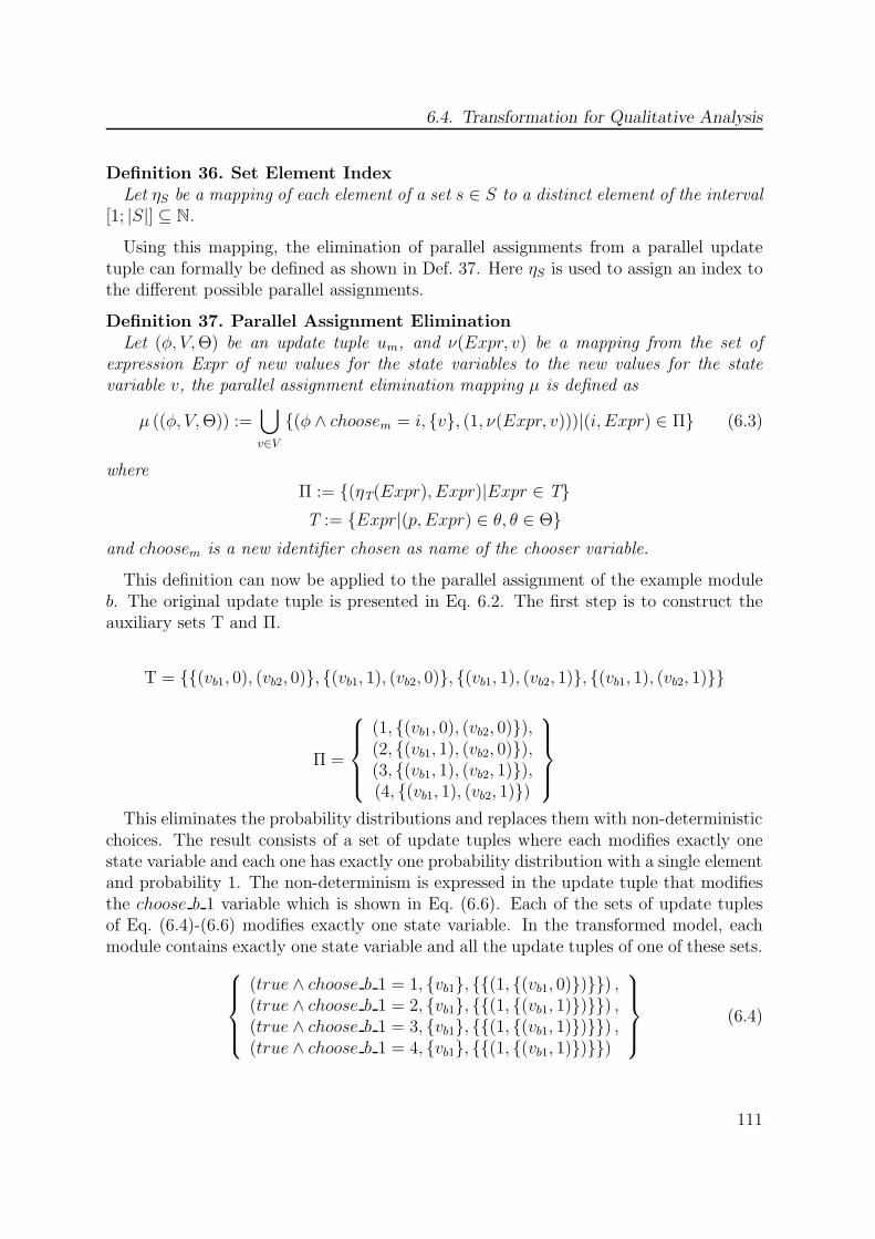
6.4. Transformation for Qualitative Analysis
Definition 36. Set Element IndexLet ηS be a mapping of each element of a set s ∈ S to a distinct element of the interval
[1; |S|] ⊆ N.
Using this mapping, the elimination of parallel assignments from a parallel updatetuple can formally be defined as shown in Def. 37. Here ηS is used to assign an index tothe different possible parallel assignments.
Definition 37. Parallel Assignment EliminationLet (φ, V,Θ) be an update tuple um, and ν(Expr, v) be a mapping from the set of
expression Expr of new values for the state variables to the new values for the statevariable v, the parallel assignment elimination mapping µ is defined as
µ ((φ, V,Θ)) :=⋃
v∈V
{(φ ∧ choosem = i, {v}, (1, ν(Expr, v)))|(i, Expr) ∈ Π} (6.3)
whereΠ := {(ηT(Expr), Expr)|Expr ∈ T}
T := {Expr|(p, Expr) ∈ θ, θ ∈ Θ}
and choosem is a new identifier chosen as name of the chooser variable.
This definition can now be applied to the parallel assignment of the example moduleb. The original update tuple is presented in Eq. 6.2. The first step is to construct theauxiliary sets T and Π.
T = {{(vb1, 0), (vb2, 0)}, {(vb1, 1), (vb2, 0)}, {(vb1, 1), (vb2, 1)}, {(vb1, 1), (vb2, 1)}}
Π =
(1, {(vb1, 0), (vb2, 0)}),(2, {(vb1, 1), (vb2, 0)}),(3, {(vb1, 1), (vb2, 1)}),(4, {(vb1, 1), (vb2, 1)})
This eliminates the probability distributions and replaces them with non-deterministicchoices. The result consists of a set of update tuples where each modifies exactly onestate variable and each one has exactly one probability distribution with a single elementand probability 1. The non-determinism is expressed in the update tuple that modifiesthe choose b 1 variable which is shown in Eq. (6.6). Each of the sets of update tuplesof Eq. (6.4)-(6.6) modifies exactly one state variable. In the transformed model, eachmodule contains exactly one state variable and all the update tuples of one of these sets.
(true ∧ choose b 1 = 1, {vb1}, {{(1, {(vb1, 0)})}}) ,(true ∧ choose b 1 = 2, {vb1}, {{(1, {(vb1, 1)})}}) ,(true ∧ choose b 1 = 3, {vb1}, {{(1, {(vb1, 1)})}}) ,(true ∧ choose b 1 = 4, {vb1}, {{(1, {(vb1, 1)})}})
(6.4)
111

6. Transformation and Analysis of SAML Models
(true ∧ choose b 1 = 1, {vb2}, {{(1, {(vb2, 0)})}}) ,(true ∧ choose b 1 = 2, {vb2}, {{(1, {(vb2, 0)})}}) ,(true ∧ choose b 1 = 4, {vb2}, {{(1, {(vb2, 1)})}}) ,(true ∧ choose b 1 = 3, {vb2}, {{(1, {(vb2, 1)})}})
(6.5)
true, {choose b 1},
{(1, {(choose b 1, 1)})}{(1, {(choose b 1, 2)})}{(1, {(choose b 1, 3)})}{(1, {(choose b 1, 4)})}
(6.6)
In summary, the parallel assignment elimination of a SAML system model for quali-tative analysis works as follows: each update rule with parallel assignments
1. is transformed using the parallel assignment elimination mapping µ (Def. 37)
2. gets an associated new chooser variable which models parallel assignments
3. defines new SAML modules, each containing exactly one of the original statevariables
This results in a partitioning of the original model into single modules with only asingle state variable and one single module for each newly introduced chooser variable.The parallel composition of this leads to a set of MDPs, each with a different initialstate, due to differing initial valuations of the chooser variables.The behavior of the resulting MDPs is identical to the behavior of the original model
with respect to the non-deterministic behavior, represented by the embedded Kripkestructures. Lemma (10) states that the paths of the original and the transformed setof MDPs in Λ are equivalent in the following sense: for each path π of the embeddedKripke structure of the original model, there exists a path π′ in one of the embeddedKripke structures of the transformed models such that for the projection of π′ onto theoriginal state variables var: π′|{var} ≡ π holds. The same holds the other way round foreach embedded Kripke structure of each of the MDPs in the set Λ.
Lemma 10. Transformation EquivalenceLet M be a SAML model with state variables v1, . . . , vk, and update rules u1 . . . um
and the corresponding MDP τMDP . Let U :=⋃m
i=1{µ(ui)} be the set of update tuples ofM with eliminated parallel assignments.Let M ′ be the parallel composition M1|| · · · ||Mk||Mchoose1|| · · · ||Mchoosem where Mi is
a SAML module with the single state variable vi and all the updates of the set U of theform (φ, vi,Θ) and Mchoosei is a SAML module with the chooser variable choosei andthe update rules for choosei from U of the form
(true, {choosei}, {{(1, {(choosei, [1, j] ⊆ N}}})
112

6.4. Transformation for Qualitative Analysis
1 e l i m i n i a t e p a r a l l e l a s s i g n (updateSetSAML)2 newStateVars := samlStateVars3 updatesNoPara l l e l := ∅4 for ( update u : updateSetSAML)5 i f hasPar a l l e lA s s i gn s (u) then6 chooseVar := getFreshVar iab le ( )7 newStateVars := newStateVars ∪ { chooseVar }8 (φ , va r i ab l eSe t , pDi s tL i s t ) := u9 for ( variableName v : variableSAML )
10 for ( i = 0 ; i < | pDi s tL i s t | ; i++)11 updatesNoPara l l e l := updatesNoPara l l e l ∪12 {(φ ∧ chooseVar = i ,{v } , [ getExpr (v , pDi s tL i s t [ i ] ) ] ) }13 updatesNoPara l l e l := updatesNoPara l l e l ∪14 {( true ,{ chooseVar } , { 0 . . | pDi s tL i s t | }}15 else16 updatesNoPara l l e l := updatesNoPara l l e l ∪ {u}17 return ( updatesNoPara l l e l )
Listing 6.2: Pseudocode to Eliminate Parallel Assignments from a Set of Update Tuples
Let Λ := {τ ′MDP} be the set of MDPs corresponding to the set of possible M ′ with a fixedinitial value for each choosei variable, then
∀π : (π ∈ Paths(κ(τMDP )) ⇔ ∃τ ′MDP ∈ Λ : π ≡ π′|{v1,...,vk} ∧ π′ ∈ Paths(κ(τ ′MDP )))
proof see p. 174
Listing 6.2 shows the pseudocode to implement the above parallel assignment elimi-nation. Its input is a set of SAML update tuples (updateSetSAML). Its output is a setof update tuples with eliminated parallel assignments and the necessary update tuplesof newly introduced state variables. The resulting set of update tuples is then used todefine new SAML modules, each holding a single state variable.
Single State Extension
As described in the last section, the simple combination of these embedded Kripkestructures of the MDPs to a single Kripke structure with multiple initial states can beproblematic. Although it is well defined, it can lead to problems with the semanticsof temporal logic specification on these Kripke structures. As mentioned before, theintended semantics of the transformations is unfortunately not equivalent to the seman-tics implemented in the verification tools. Therefore an additional initial state whichcombines the set of MDPs into a single one is introduced as follows:
113
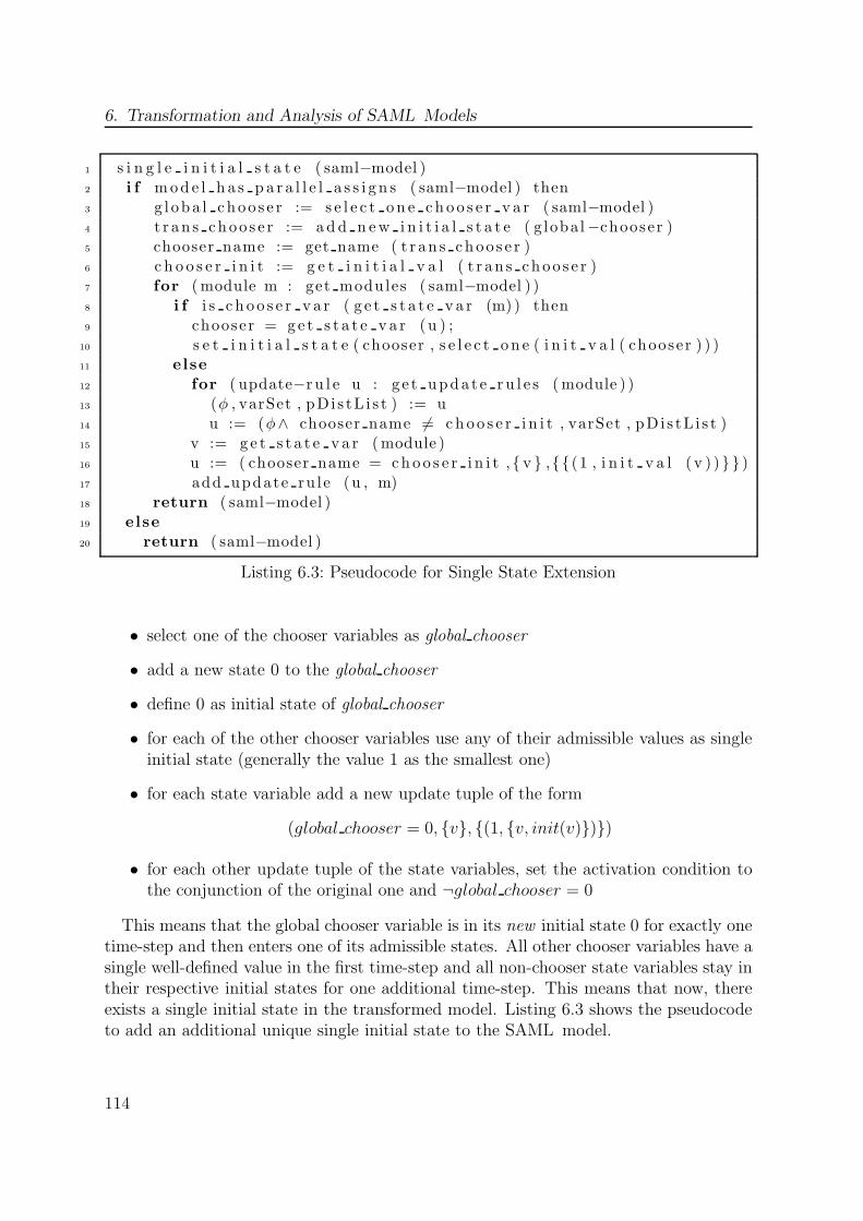
6. Transformation and Analysis of SAML Models
1 s i n g l e i n i t i a l s t a t e ( saml−model )2 i f mod e l h a s p a r a l l e l a s s i g n s ( saml−model ) then3 g l oba l ch oo s e r := s e l e c t on e ch oo s e r v a r ( saml−model )4 t r an s choo s e r := ad d n ew i n i t i a l s t a t e ( g lobal−chooser )5 chooser name := get name ( t r an s choo s e r )6 c h o o s e r i n i t := g e t i n i t i a l v a l ( t r an s choo s e r )7 for (module m : get modules ( saml−model ) )8 i f i s c h o o s e r v a r ( g e t s t a t e v a r (m) ) then9 chooser = g e t s t a t e v a r (u ) ;
10 s e t i n i t i a l s t a t e ( chooser , s e l e c t on e ( i n i t v a l ( chooser ) ) )11 else12 for ( update−r u l e u : g e t upda t e r u l e s (module ) )13 (φ , varSet , pDi s tL i s t ) := u14 u := (φ∧ chooser name 6= choo s e r i n i t , varSet , pDi s tL i s t )15 v := g e t s t a t e v a r (module )16 u := ( chooser name = ch oo s e r i n i t ,{ v } ,{{(1 , i n i t v a l ( v ) )}} )17 add update ru le (u , m)18 return ( saml−model )19 else20 return ( saml−model )
Listing 6.3: Pseudocode for Single State Extension
• select one of the chooser variables as global chooser
• add a new state 0 to the global chooser
• define 0 as initial state of global chooser
• for each of the other chooser variables use any of their admissible values as singleinitial state (generally the value 1 as the smallest one)
• for each state variable add a new update tuple of the form
(global chooser = 0, {v}, {(1, {v, init(v)})})
• for each other update tuple of the state variables, set the activation condition tothe conjunction of the original one and ¬global chooser = 0
This means that the global chooser variable is in its new initial state 0 for exactly onetime-step and then enters one of its admissible states. All other chooser variables have asingle well-defined value in the first time-step and all non-chooser state variables stay intheir respective initial states for one additional time-step. This means that now, thereexists a single initial state in the transformed model. Listing 6.3 shows the pseudocodeto add an additional unique single initial state to the SAML model.
114

6.4. Transformation for Qualitative Analysis
This construction leads to a new single initial state s−1 of the embedded Kripkestructure from which any of the original initial states of the set S0 can be reached in onetime-step via a non-deterministic choice. In particular this means for a SAML modelMand a SAML model M ′ which is the result from the transformation as described above,that for each path of the embedded Kripke structure of M ′, the postfix of this path hasan equivalent path in the embedded Kripke structure ofM and vice versa. This is shownin Lemma (11).
Lemma 11. Single Initial State ExtensionLet M be a SAML model with state variables v1 . . . vk and M ′ the SAML model which
results from parallel assignment elimination and single state extension of M , then
∀π : (π = s0s1 . . . ∈ Paths(κ(M))
⇔ ∃π′ = s′−1s′0 . . . ∈ Paths(κ(M ′)) : s0 ≡ s′−1|v1,...,vk ∧ ∀i ≥ 0 : si ≡ s′i|v1,...,vk)
proof see p. 175
In general this additional initial state must be reflected in the temporal logic proofobligations. But as the transformation is done in such a way that the values of allnon-chooser state variables of the original model in s−1 are exactly the same as in states0, all the qualitative safety analysis methods presented in Section 5.2 are equivalenton both models. The reason for this is that they consist of reachability analyses andthe construction does not change the reachable states (for v1 . . . vk), but only delayseverything for one time-step. The safety analysis proof obligations do also not containBoolean expression over the values of the chooser variables.Nevertheless this effect must be accounted for if other temporal logic properties should
be checked. Then the one time-step delay must be considered by using the next operatorto skip the new initial state. For an LTL formula φ, this will generally simply be theformula X(φ). For CTL formulas, it is a bit trickier. The intended semantics of anexistentially quantified ψE formula is that “there exists an initial state such that ψE
holds”. This can be accounted for with EX(ψE), i.e. there exists a state s0 reachablein one time-step from s−1 such that ψE holds. For an always quantified formula ψA,the intended semantics is “ψA holds for all possible initial states”. This can analogouslybe expressed in the transformed model as AX(ψA). Note, that parsing and automatictransformation of temporal logic specifications is not implemented at the moment, butsuch an implementation would be rather straightforward.For practical purposes, the addition of the new initial state seems to be a more con-
venient solution than to check every temporal logic property on the multiple Kripkestructures resulting from the parallel assignment elimination. Yet it should be notedthat other possible semantically sound transformations of SAML models for qualitativesafety analysis are conceivable.For the concrete verification of qualitative properties on the transformed model, it now
only has to be expressed in an appropriate format for a verification tool like NuSMV.
115
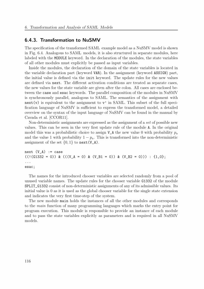
6. Transformation and Analysis of SAML Models
6.4.3. Transformation to NuSMV
The specification of the transformed SAML example model as a NuSMV model is shownin Fig. 6.4. Analogous to SAML models, it is also structured in separate modules, herelabeled with the MODULE keyword. In the declaration of the modules, the state variablesof all other modules must explicitly be passed as input variables.Inside the modules, the declaration of the domain of the state variables is located in
the variable declaration part (keyword VAR). In the assignment (keyword ASSIGN) part,the initial value is defined via the init keyword. The update rules for the new valuesare defined via next. The different activation conditions are treated as separate cases,the new values for the state variable are given after the colon. All cases are enclosed be-tween the case and esac keywords. The parallel composition of the modules in NuSMVis synchronously parallel, analogous to SAML. The semantics of the assignment withnext(v) is equivalent to the assignment to v’ in SAML. This subset of the full speci-fication language of NuSMV is sufficient to express the transformed model, a detailedoverview on the syntax of the input language of NuSMV can be found in the manual byCavada et al. [CCOR11].Non-deterministic assignments are expressed as the assignment of a set of possible new
values. This can be seen in the very first update rule of the module A. In the originalmodel this was a probabilistic choice to assign V_A the new value 0 with probability paand the value 1 with probability 1− pa. This is transformed into the non-deterministicassignment of the set {0, 1} to next(V_A).
next (V_A) := case
((!(G1332 = 0)) & (((V_A = 0) & (V_B1 = 0)) & (V_B2 = 0))) : {1,0};
...
esac;
The names for the introduced chooser variables are selected randomly from a pool ofunused variable names. The update rules for the chooser variable G1332 of the moduleSPLIT_G1332 consist of non-deterministic assignments of any of its admissible values. Itsinitial value is 0 as it is used as the global chooser variable for the single state extensionand indicates the very first time-step of the system.The new module main holds the instances of all the other modules and corresponds
to the main function of many programming languages which marks the entry point forprogram execution. This module is responsible to provide an instance of each moduleand to pass the state variables explicitly as parameters and is required in all NuSMVmodels.
116
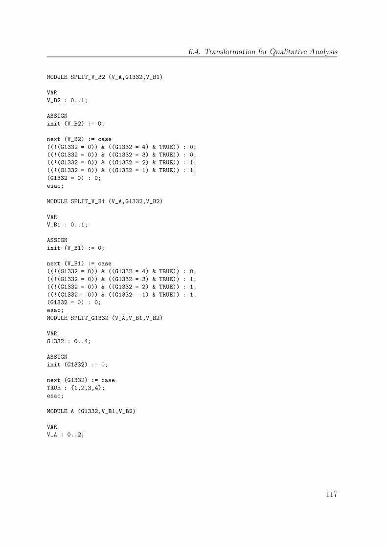
6.4. Transformation for Qualitative Analysis
MODULE SPLIT_V_B2 (V_A,G1332,V_B1)
VAR
V_B2 : 0..1;
ASSIGN
init (V_B2) := 0;
next (V_B2) := case
((!(G1332 = 0)) & ((G1332 = 4) & TRUE)) : 0;
((!(G1332 = 0)) & ((G1332 = 3) & TRUE)) : 0;
((!(G1332 = 0)) & ((G1332 = 2) & TRUE)) : 1;
((!(G1332 = 0)) & ((G1332 = 1) & TRUE)) : 1;
(G1332 = 0) : 0;
esac;
MODULE SPLIT_V_B1 (V_A,G1332,V_B2)
VAR
V_B1 : 0..1;
ASSIGN
init (V_B1) := 0;
next (V_B1) := case
((!(G1332 = 0)) & ((G1332 = 4) & TRUE)) : 0;
((!(G1332 = 0)) & ((G1332 = 3) & TRUE)) : 1;
((!(G1332 = 0)) & ((G1332 = 2) & TRUE)) : 1;
((!(G1332 = 0)) & ((G1332 = 1) & TRUE)) : 1;
(G1332 = 0) : 0;
esac;
MODULE SPLIT_G1332 (V_A,V_B1,V_B2)
VAR
G1332 : 0..4;
ASSIGN
init (G1332) := 0;
next (G1332) := case
TRUE : {1,2,3,4};
esac;
MODULE A (G1332,V_B1,V_B2)
VAR
V_A : 0..2;
117
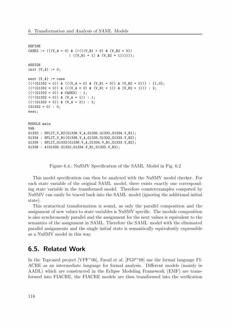
6. Transformation and Analysis of SAML Models
DEFINE
CASE3 := (((V_A = 0) & (!(((V_B1 = 0) & (V_B2 = 0))
| ((V_B1 = 1) & (V_B2 = 1))))));
ASSIGN
init (V_A) := 0;
next (V_A) := case
((!(G1332 = 0)) & (((V_A = 0) & (V_B1 = 0)) & (V_B2 = 0))) : {1,0};
((!(G1332 = 0)) & (((V_A = 0) & (V_B1 = 1)) & (V_B2 = 1))) : 2;
((!(G1332 = 0)) & CASE3) : 1;
((!(G1332 = 0)) & (V_A = 1)) : 1;
((!(G1332 = 0)) & (V_A = 2)) : 2;
(G1332 = 0) : 0;
esac;
MODULE main
VAR
G1333 : SPLIT_V_B2(G1336.V_A,G1335.G1332,G1334.V_B1);
G1334 : SPLIT_V_B1(G1336.V_A,G1335.G1332,G1333.V_B2);
G1335 : SPLIT_G1332(G1336.V_A,G1334.V_B1,G1333.V_B2);
G1336 : A(G1335.G1332,G1334.V_B1,G1333.V_B2);
Figure 6.4.: NuSMV Specification of the SAML Model in Fig. 6.2
This model specification can then be analyzed with the NuSMV model checker. Foreach state variable of the original SAML model, there exists exactly one correspond-ing state variable in the transformed model. Therefore counterexamples computed byNuSMV can easily be traced back into the SAML model (ignoring the additional initialstate).This syntactical transformation is sound, as only the parallel composition and the
assignment of new values to state variables is NuSMV specific. The module compositionis also synchronously parallel and the assignment for the next values is equivalent to thesemantics of the assignment in SAML. Therefore the SAML model with the eliminatedparallel assignments and the single initial state is semantically equivalently expressibleas a NuSMV model in this way.
6.5. Related Work
In the Topcased project [VPF+06], Farail et al. [FGP+08] use the formal language FI-ACRE as an intermediate language for formal analysis. Different models (mainly inAADL) which are constructed in the Eclipse Modeling Framework (EMF) are trans-formed into FIACRE, the FIACRE models are then transformed into the verification
118

6.5. Related Work
tools of the CADP toolbox developed by Fernandez et al. [FGK+96] or the TINA petrinet analyzer developed by Berthomieu et al. [BaFV04]. Due to the amount of model-ing artifacts that are supported in FICARE, only structural properties of systems canbe proven, the models are too complex for a successful verification of behavioral as-pects [FGP+08]. SAML has deliberately been designed to be as simple as possible forformal analysis while retaining the expressiveness needed for extended system modeling.
The SLIM formalization by Bozzano et al. [BCK+09b] of an AADL subset and theAADL error annex [SA06] developed in the COMPASS project [BCK+10b] can alsotransformed into different analysis tools for either qualitative or quantitative analysis.SLIM separates the specification in nominal and failure parts. The nominal part, whichcan also include continuous variables with change rate in addition to discrete statevariables, is transformed into a variant of the NuSMV model checker which also supportssatisfiability modulo theory (SMT) solving techniques that can solve such hybrid systembehavior. This is achieved by the integration of the MathSAT SAT solver developed byBruttomesso et al. [BCF+08] into the COMPASS toolchain.
The probabilistic failure modeling uses continuous time models which are analyzedwith the MRMC model-checker. This is called performability analysis in COMPASS.The transformation consists of two steps: firstly, the state space of the SLIM model isgenerated. The semantics allows instantaneous transitions which are not probabilisticand do not consume time and therefore are of no effect on the quantitative model. Ina second step, all states resulting from such transitions are collapsed together using the“lumping” mechanism. This is conducted using bisimulation minimization of the labeledtransition system with the SigRef tool developed by Wimmer et al. [WHH+06] in theAVACS project. Nevertheless, this performability analysis is only possible on modelsthat do not express such hybrid behavior [Ngu10]. The necessary transformations forSLIM are realized on the semantic level and are directly integrated into the verifica-tions tools (NuSMV and MRMC are developed by groups participating in COMPASS).Therefore it is not easily possible to use other verification tools for the analyses (e.g. likePRISM for quantitative analysis of larger models) as with the tool-independent approachbased on SAML.
Summary
This chapter presented model transformations which allow for safety analysis of ex-tended SAML models with different verification tools. At the same time, they guaran-tee that the transformed models are equivalent in some sense, rendering the approachtool-independent. Therefore it benefits directly from improved analysis tools and it isalso possible to add newly developed analysis tools. The currently implemented trans-formations allow to use PRISM and MRMC for quantitative analysis and NuSMV andCadence SMV for qualitative analysis. The transformations are on the syntactical level,which facilitates the integration of additional verification tools.
119

6. Transformation and Analysis of SAML Models
The transformations of SAML models into the input language of PRISM requires theexplicit synchronization of the update rules and the transformation of non-deterministicchoices into update rules with equivalent activation conditions.The transformation for qualitative analysis is more complex. Many analysis tools do
not allow for parallel assignments for multiple state variables which is possible in SAML.This problem was solved by the introduction of one additional state variable per parallelassignments that signals which possibility was chosen. The result of this transformationis a set of SAML models, for which path inclusion equivalency holds. It is possibleto combine this set of models into a single equivalent model of a Kripke structure, onwhich all of the qualitative model-based safety analyses can be conducted. This can beanalyzed using qualitative verification tools like the different SMV variants.
120
7. Case Studies
Programming is usually taught by examples.
(Niklaus Wirth)
This chapter presents three case studies which are analyzed using the formal model-based analysis methods presented in the previous chapter. It describes how systems fromdifferent application domains can be modeled and analyzed. The chapter discusses ad-vantages as well as limitations of the modeling and model-based safety analysis methodspresented in this dissertation. The results of the analysis of each case study are pre-sented, as well as information about the computational effort that is required to conductthe analyses.A larger industrial case study from the railway domain is described in Section 7.1.
Section 7.2 presents the full modeling of the case study which was used in Chapter 4 andChapter 5. Section 7.3 discusses a case study of a self-healing system from productionautomation. Section 7.4 concludes the chapter with some discussion about related workon the selected case studies.
121
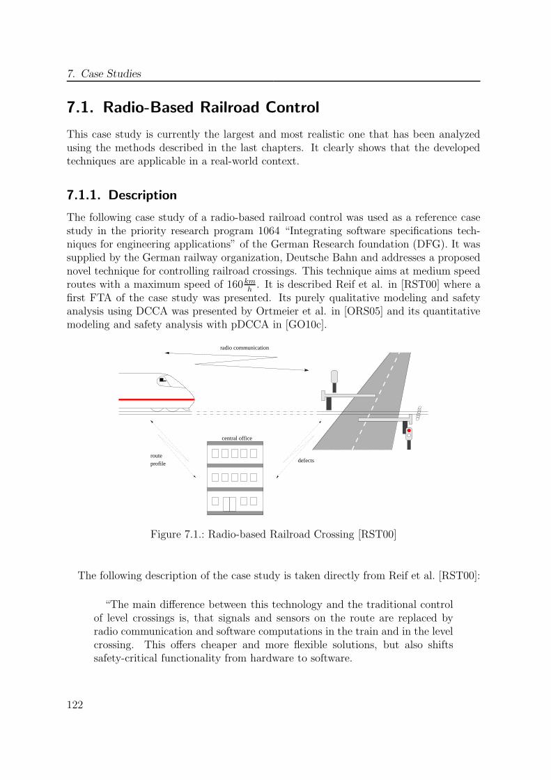
7. Case Studies
7.1. Radio-Based Railroad Control
This case study is currently the largest and most realistic one that has been analyzedusing the methods described in the last chapters. It clearly shows that the developedtechniques are applicable in a real-world context.
7.1.1. Description
The following case study of a radio-based railroad control was used as a reference casestudy in the priority research program 1064 “Integrating software specifications tech-niques for engineering applications” of the German Research foundation (DFG). It wassupplied by the German railway organization, Deutsche Bahn and addresses a proposednovel technique for controlling railroad crossings. This technique aims at medium speedroutes with a maximum speed of 160km
h. It is described Reif et al. in [RST00] where a
first FTA of the case study was presented. Its purely qualitative modeling and safetyanalysis using DCCA was presented by Ortmeier et al. in [ORS05] and its quantitativemodeling and safety analysis with pDCCA in [GO10c].
radio communication
central office
routeprofile defects
Figure 7.1.: Radio-based Railroad Crossing [RST00]
The following description of the case study is taken directly from Reif et al. [RST00]:
“The main difference between this technology and the traditional controlof level crossings is, that signals and sensors on the route are replaced byradio communication and software computations in the train and in the levelcrossing. This offers cheaper and more flexible solutions, but also shiftssafety-critical functionality from hardware to software.
122
7.1. Radio-Based Railroad Control
Instead of detecting an approaching train by a sensor, the train computesthe position where it has to send a signal to secure the level crossing. There-fore the train has to know the position of the level crossing, the time neededto secure the level crossing, and its current speed and position, which ismeasured by an odometer.When the level crossing receives this command, it switches on the traffic
lights, first the yellow light, then the red light, and finally closes the barri-ers. When they are closed, the level crossing is safe for a certain period oftime. The stop signal, indicating an insecure crossing, is also substituted bycomputation and communication. The train requests the status of the levelcrossing. Depending on the answer the train will brake or pass the crossing.The level crossing periodically performs self-diagnosis and automatically in-forms the central office about defects and problems. The central office isresponsible for repair and provides route descriptions for trains. These de-scriptions indicate the positions of level crossings and maximum speed onthe route.”
For the formal modeling in SAML and model-based safety analysis, the case study isadapted as follows: The train continuously monitors its position and its speed via theodometer. When it approaches the crossing, it initiates the communication by sendinga secure request. When the crossing receives this, it starts closing the barrier. Shortlybefore the train reaches the latest braking point – the smallest distance to the barrierwhere it is possible for the train to stop in front of the crossing with its current speed –it requests the status of the crossing. The crossing acknowledges this signal if the sensorat the barrier detects that the barrier is closed. If there is no secured signal, the trainbrakes immediately. The passing of the train is detected by a sensor located after thecrossing, allowing the crossing to reopen the barrier. The central office was not modeledfor the analysis.
7.1.2. Modeling
The structure of the modeling of the case study is similar to the original modeling forStatecharts presented by Ortmeier et al. [ORS05]. But of course, here the quantitativeinformation is directly integrated into the extended system model. In return, a moreaccurate modeling of the case study, in particular of the probabilistic failure mode mod-eling and of the physical environment, and a more accurate quantitative analysis withpDCCA is possible.
Modeling of Hardware and Software
The hardware and software modeling in this case study is the crossing itself which ismodeled by its states, the crossing control which is responsible to control the statechanges of the crossing and the control of the train.
123

7. Case Studies
Crossing The control of the crossing is triggered by signals from the communicationwith the approaching train. The module representing the crossing is shown in Fig. 7.2.The state variable crossing has three possible states: an opened state which is alsothe initial state, a closing state and a fully closed state. The state opened is left whenthe activation condition close holds, which means that the train has sent its closingrequest to the crossing and the request has been received. This also starts an (external)timer and the crossing is in state closing as long as the timer counts (timer1 > 0). Theclosing of the barrier of the crossing needs some time, 30s in the model of the case study.When this has passed, the crossing enters state closed. This starts another timer andthe crossing gets opened again (enters state opened) when either a predefined amountof time elapses (timer2 = 0)1 or the trainPassed signal arrives which announces thatthe train has passed the crossing.
Module Crossing / crossing
opened
closing closed
1
¬timer1 = 0
1timer1 = 0
1
1
1
1
Close
¬Close
¬(timer2 = 0 ∨ trainPassed)
timer2 = 0 ∨ trainPassed
Figure 7.2.: Original Crossing Model
Train Control The behavior of the train is defined by the train control. It modelsthe current state of the train. The train control continuously monitors the speed of thetrain as well as its position and initiates the communication with the crossing in suchway that it can still stop before the dangerous position if the crossing is not closed. Tocompute the positions from where to initiate the communication and when to brake ifthere is no answer received, the train uses the reading from the odometer of the traincalled virtual speed.
1This is a requirement from the Deutsche Bahn to assure that people who become impatient after along waiting and decide to cross the track anyway do so at least fast.
124
7.1. Radio-Based Railroad Control
The corresponding module is shown in Fig. 7.3. It consists of the state variabletrainControl. Its initial state is idle which means that the train approaches the cross-ing. When the train determines that the position to initiate the closing of the crossing isreached (posCloseReached holds), it enters the state waitClose where it stays until thestatus reporting position has been reached at which it requests the state of the barrier ofthe crossing. It then enters the state waitSig where it stays until either the crossing sig-nals that it is closed (ackReceived holds) or the last breaking position has been reached(posBrakeReached holds). If the crossing signals its closed state, the train enters theok state and passes the crossing without braking.
If the last breaking position has been reached without a signal from the crossing, thetrain brakes to prevent entering the crossing and the state of the train control is set tobrake. All the positions are not fixed, but are computed by the train control dependenton the virtual speed reading of the odometer.
Module TrainControl / trainControl
ok
brake
waitSig
idle
waitClose
1
1
11
1
1
¬posCloseReached
true
true
1
¬posStatusReached
¬(ackReceived ∨ posBrakeReached)
1
posBrakeReached
1
posStatusReached
posCloseReached
¬posBrakereached
∧ackReceived
Figure 7.3.: Train Control
Modeling of Physical Behavior
The modeling of the physical behavior of the train covers mainly its movement. In orderto be realistic, not only the current position and velocity must be considered, but alsothe modeling of acceleration and deceleration (braking). This is separated into three
125
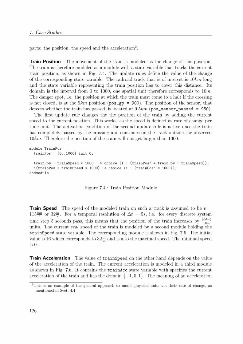
7. Case Studies
parts: the position, the speed and the acceleration2.
Train Position The movement of the train is modeled as the change of this position.The train is therefore modeled as a module with a state variable that tracks the currenttrain position, as shown in Fig. 7.4. The update rules define the value of the changeof the corresponding state variable. The railroad track that is of interest is 10km longand the state variable representing the train position has to cover this distance. Itsdomain is the interval from 0 to 1000, one spatial unit therefore corresponds to 10m.The danger spot, i.e. the position at which the train must come to a halt if the crossingis not closed, is at the 9km position (pos_gp = 900). The position of the sensor, thatdetects whether the train has passed, is located at 9.5km (pos_sensor_passed = 950).The first update rule changes the the position of the train by adding the current
speed to the current position. This works, as the speed is defined as rate of change pertime-unit. The activation condition of the second update rule is active once the trainhas completely passed by the crossing and continues on the track outside the observed10km. Therefore the position of the train will not get larger than 1000.
module TrainPos
trainPos : [0..1000] init 0;
trainPos + trainSpeed < 1000 -> choice (1 : (trainPos’ = trainPos + trainSpeed));
!(trainPos + trainSpeed < 1000) -> choice (1 : (trainPos’ = 1000));
endmodule
Figure 7.4.: Train Position Module
Train Speed The speed of the modeled train on such a track is assumed to be v =115km
hor 32m
s. For a temporal resolution of ∆t = 5s, i.e. for every discrete system
time step 5 seconds pass, this means that the position of the train increases by (∆t·v)10m
units. The current real speed of the train is modeled by a second module holding thetrainSpeed state variable. The corresponding module is shown in Fig. 7.5. The initialvalue is 16 which corresponds to 32m
sand is also the maximal speed. The minimal speed
is 0.
Train Acceleration The value of trainSpeed on the other hand depends on the valueof the acceleration of the train. The current acceleration is modeled in a third moduleas shown in Fig. 7.6. It contains the trainAcc state variable with specifies the currentacceleration of the train and has the domain {−1, 0, 1}. The meaning of an acceleration
2This is an example of the general approach to model physical units via their rate of change, asmentioned in Sect. 4.4
126

7.1. Radio-Based Railroad Control
module TrainSpeed
trainSpeed : [0..16] init 16;
(trainSpeed + trainAcc < 0) -> choice (1 : (trainSpeed’ = 0));
(trainSpeed + trainAcc > 16) -> choice (1 : (trainSpeed’ = 16));
!(trainSpeed + trainAcc < 0 | trainSpeed + trainAcc > 16) ->
choice (1 : (trainSpeed’ = trainSpeed + trainAcc));
endmodule
Figure 7.5.: Train Speed Module
of value 1 is that trainSpeed changes 1 unit in one time-step. As one trainSpeed
unit corresponds to 2msand ∆t = 5s this means that if trainAcc has the value 1, the
acceleration is 25ms2
(and −25ms2
for the deceleration with trainAcc = -1).
0
−1
1
Module TrainAccel / trainAcc
trainControl 6= brake
1
trainControl = brake
1
1
trainControl = brake
trainControl = brake
trainControl 6= brake
trainControl 6= brake
Figure 7.6.: Train Acceleration Module
Modeling of Failure Modes
In this case study, different failure modes are possible. The relevant ones for the safetyanalysis are the following: failure of the brakes (error brake) which models that the traindoes not decelerate as intended, failure of the communication between the train and thecrossing (error comm), failure of the crossing closed sensor (error closed) which results inwrongly signaling a closed barrier, failure of the actuator of the barrier (error actuator)which means that the barrier does not close as intended, failure of the sensor that detects
127
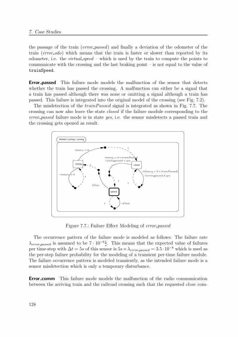
7. Case Studies
the passage of the train (error passed) and finally a deviation of the odometer of thetrain (error odo) which means that the train is faster or slower than reported by itsodometer, i.e. the virtual speed – which is used by the train to compute the points tocommunicate with the crossing and the last braking point – is not equal to the value oftrainSpeed.
Error passed This failure mode models the malfunction of the sensor that detectswhether the train has passed the crossing. A malfunction can either be a signal thata train has passed although there was none or omitting a signal although a train haspassed. This failure is integrated into the original model of the crossing (see Fig. 7.2).The misdetection of the trainPassed signal is integrated as shown in Fig. 7.7. The
crossing can now also leave the state closed if the failure module corresponding to theerror passed failure mode is in state yes, i.e. the sensor misdetects a passed train andthe crossing gets opened as result.
Module Crossing / crossing
closing
opened
closed
1
¬timer1 = 0
1timer1 = 0
timer2 = 0 ∨ trainPassed
1
1
1
1
Close
¬Close
∧error passed 6= yes
∨fails passed = yes
¬(timer2 = 0 ∨ trainPassed)
Figure 7.7.: Failure Effect Modeling of error passed
The occurrence pattern of the failure mode is modeled as follows: The failure rateλerror passed is assumed to be 7 · 10−9 1
s. This means that the expected value of failures
per time-step with ∆t = 5s of this sensor is 5s×λerror passed = 3.5 ·10−8 which is used asthe per-step failure probability for the modeling of a transient per-time failure module.The failure occurrence pattern is modeled transiently, as the intended failure mode is asensor misdetection which is only a temporary disturbance.
Error comm This failure mode models the malfunction of the radio communicationbetween the arriving train and the railroad crossing such that the requested close com-
128
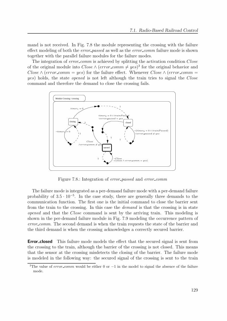
7.1. Radio-Based Railroad Control
mand is not received. In Fig. 7.8 the module representing the crossing with the failureeffect modeling of both the error passed as well as the error comm failure mode is showntogether with the parallel failure modules for the failure modes.The integration of error comm is achieved by splitting the activation condition Close
of the original module into Close ∧ (error comm 6= yes)3 for the original behavior andClose ∧ (error comm = yes) for the failure effect. Whenever Close ∧ (error comm =yes) holds, the state opened is not left although the train tries to signal the Closecommand and therefore the demand to close the crossing fails.
Module Crossing / crossing
closing closed
opened
∧error passed 6= yes
¬(timer2 = 0 ∧ trainPassed)
1
¬timer1 = 0
1timer1 = 0
timer2 = 0 ∨ trainPassed
1
1
1
1
Close
¬Close∨(close ∧ error comm = yes)
∧error comm 6= yes
∨error passed = yes
Figure 7.8.: Integration of error passed and error comm
The failure mode is integrated as a per-demand failure mode with a per-demand failureprobability of 3.5 · 10−5. In the case study, there are generally three demands to thecommunication function. The first one is the initial command to close the barrier sentfrom the train to the crossing. In this case the demand is that the crossing is in stateopened and that the Close command is sent by the arriving train. This modeling isshown in the per-demand failure module in Fig. 7.9 modeling the occurrence pattern oferror comm. The second demand is when the train requests the state of the barrier andthe third demand is when the crossing acknowledges a correctly secured barrier.
Error closed This failure mode models the effect that the secured signal is sent fromthe crossing to the train, although the barrier of the crossing is not closed. This meansthat the sensor at the crossing misdetects the closing of the barrier. The failure modeis modeled in the following way: the secured signal of the crossing is sent to the train
3The value of error comm would be either 0 or −1 in the model to signal the absence of the failuremode.
129
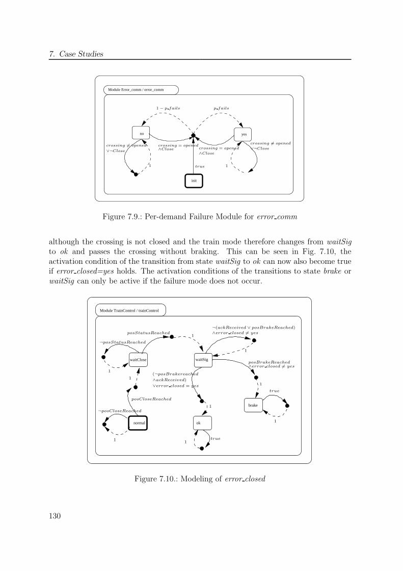
7. Case Studies
init
no yes
Module Error_comm / error_comm
1
1 − p fails p fails
∧Closecrossing 6= opened crossing = opened
∨¬Close
1true
crossing 6= opened
∨¬Closecrossing = opened
∧Close
Figure 7.9.: Per-demand Failure Module for error comm
although the crossing is not closed and the train mode therefore changes from waitSigto ok and passes the crossing without braking. This can be seen in Fig. 7.10, theactivation condition of the transition from state waitSig to ok can now also become trueif error closed=yes holds. The activation conditions of the transitions to state brake orwaitSig can only be active if the failure mode does not occur.
normal ok
brake
waitSigwaitClose
Module TrainControl / trainControl
1
1
11
1
1
¬posCloseReached
true
true
1
¬posStatusReached
posCloseReached
1
¬(ackReceived ∨ posBrakeReached)
posBrakeReached
1
∧error closed 6= yes
∧error closed 6= yes
posStatusReached
(¬posBrakereached
∧ackReceived)
∨error closed = yes
Figure 7.10.: Modeling of error closed
130
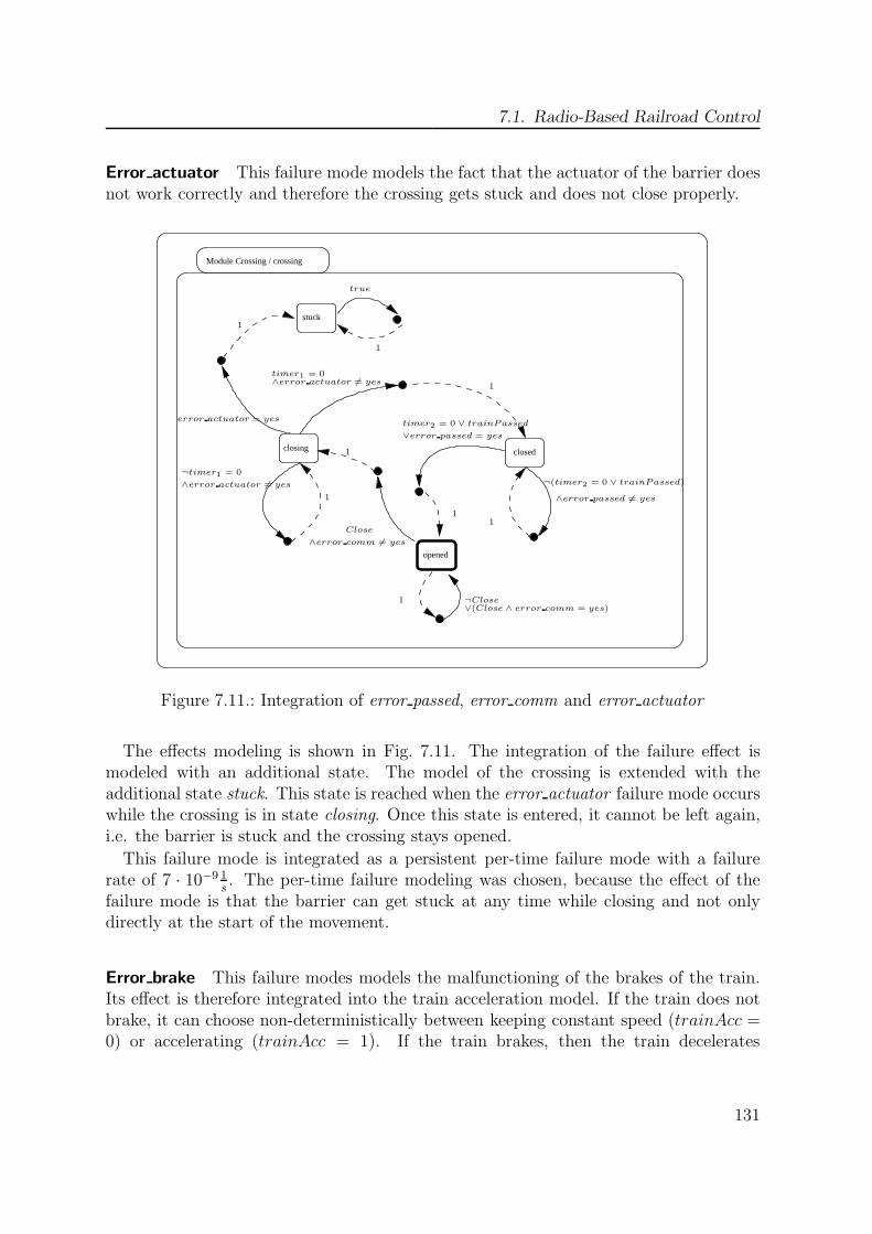
7.1. Radio-Based Railroad Control
Error actuator This failure mode models the fact that the actuator of the barrier doesnot work correctly and therefore the crossing gets stuck and does not close properly.
Module Crossing / crossing
closing closed
stuck
opened
1
1
timer2 = 0 ∨ trainPassed
1
1
1
1
¬Close
1
1
true
∧error passed 6= yes
∨(Close ∧ error comm = yes)
∨error passed = yes
¬(timer2 = 0 ∨ trainPassed)
∧error actuator 6= yestimer1 = 0
¬timer1 = 0
∧error actuator 6= yes
error actuator = yes
Close
∧error comm 6= yes
Figure 7.11.: Integration of error passed, error comm and error actuator
The effects modeling is shown in Fig. 7.11. The integration of the failure effect ismodeled with an additional state. The model of the crossing is extended with theadditional state stuck. This state is reached when the error actuator failure mode occurswhile the crossing is in state closing. Once this state is entered, it cannot be left again,i.e. the barrier is stuck and the crossing stays opened.
This failure mode is integrated as a persistent per-time failure mode with a failurerate of 7 · 10−9 1
s. The per-time failure modeling was chosen, because the effect of the
failure mode is that the barrier can get stuck at any time while closing and not onlydirectly at the start of the movement.
Error brake This failure modes models the malfunctioning of the brakes of the train.Its effect is therefore integrated into the train acceleration model. If the train does notbrake, it can choose non-deterministically between keeping constant speed (trainAcc =0) or accelerating (trainAcc = 1). If the train brakes, then the train decelerates
131
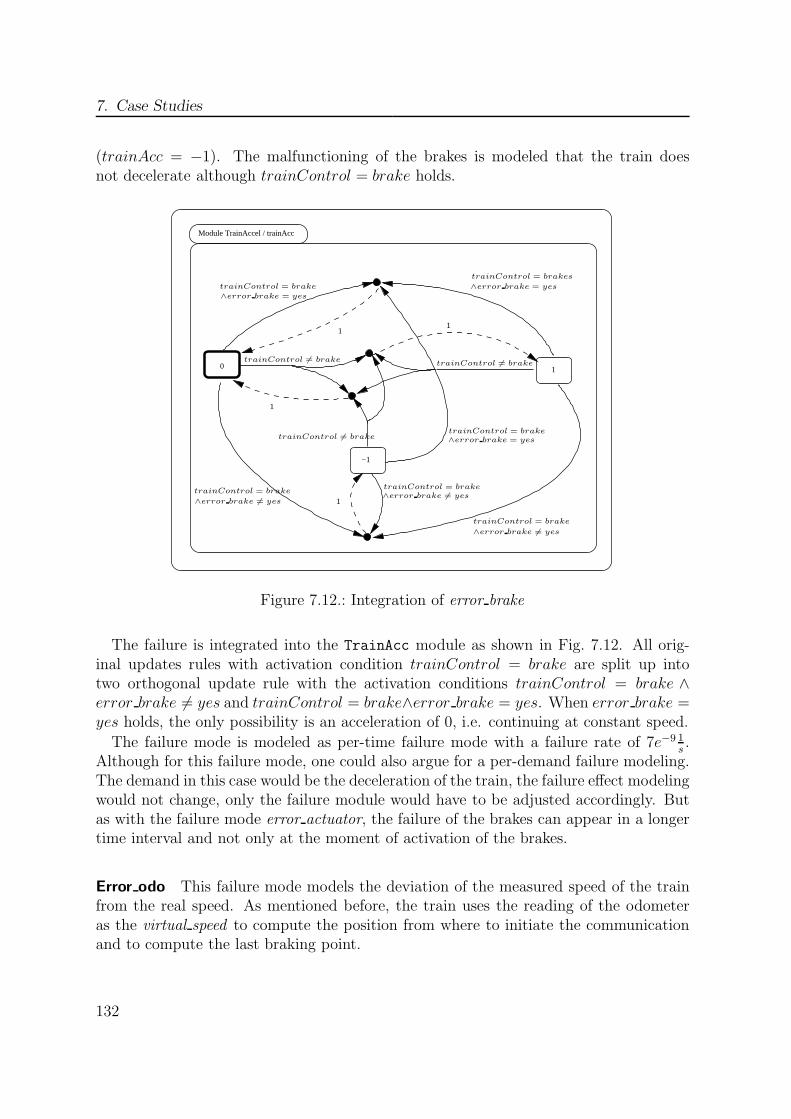
7. Case Studies
(trainAcc = −1). The malfunctioning of the brakes is modeled that the train doesnot decelerate although trainControl = brake holds.
0
−1
1
Module TrainAccel / trainAcc
∧error brake 6= yes
trainControl = brakes
∧error brake = yestrainControl = brake
∧error brake = yes
trainControl 6= brake
trainControl 6= brake
1
1
trainControl = brake∧error brake 6= yes
trainControl = brake
∧error brake 6= yes
trainControl = brake∧error brake = yes
1
1
trainControl 6= brake
trainControl = brake
Figure 7.12.: Integration of error brake
The failure is integrated into the TrainAcc module as shown in Fig. 7.12. All orig-inal updates rules with activation condition trainControl = brake are split up intotwo orthogonal update rule with the activation conditions trainControl = brake ∧error brake 6= yes and trainControl = brake∧error brake = yes. When error brake =yes holds, the only possibility is an acceleration of 0, i.e. continuing at constant speed.
The failure mode is modeled as per-time failure mode with a failure rate of 7e−9 1s.
Although for this failure mode, one could also argue for a per-demand failure modeling.The demand in this case would be the deceleration of the train, the failure effect modelingwould not change, only the failure module would have to be adjusted accordingly. Butas with the failure mode error actuator, the failure of the brakes can appear in a longertime interval and not only at the moment of activation of the brakes.
Error odo This failure mode models the deviation of the measured speed of the trainfrom the real speed. As mentioned before, the train uses the reading of the odometeras the virtual speed to compute the position from where to initiate the communicationand to compute the last braking point.
132
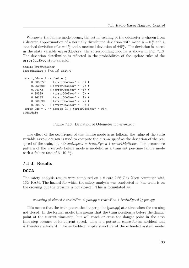
7.1. Radio-Based Railroad Control
Whenever the failure mode occurs, the actual reading of the odometer is chosen froma discrete approximation of a normally distributed deviation with mean µ = 0m
sand a
standard deviation of σ = 4msand a maximal deviation of ±6m
s. The deviation is stored
in the state variable errorOdoSkew, the corresponding module is shown in Fig. 7.13.The deviation distribution is reflected in the probabilities of the update rules of theerrorOdoSkew state variable.
module ErrorOdoSkew
errorOdoSkew : [-3..3] init 0;
error_Odo = 1 -> choice (
0.0059770 : (errorOdoSkew’ = -3) +
0.060598 : (errorOdoSkew’ = -2) +
0.24173 : (errorOdoSkew’ = -1) +
0.38339 : (errorOdoSkew’ = 0) +
0.24173 : (errorOdoSkew’ = 1) +
0.060598 : (errorOdoSkew’ = 2) +
0.0059770 : (errorOdoSkew’ = 3));
error_Odo = 0 -> choice (1 : (errorOdoSkew’ = 0));
endmodule
Figure 7.13.: Deviation of Odometer for error odo
The effect of the occurrence of this failure mode is as follows: the value of the statevariable errorOdoSkew is used to compute the virtual speed as the deviation of the realspeed of the train, i.e. virtual speed = trainSpeed + errorOdoSkew. The occurrencepattern of the error odo failure mode is modeled as a transient per-time failure modewith a failure rate of 6 · 10−5 1
s.
7.1.3. Results
DCCA
The safety analysis results were computed on a 8 core 2.66 Ghz Xeon computer with16G RAM. The hazard for which the safety analysis was conducted is “the train is onthe crossing but the crossing is not closed”. This is formulated as:
crossing 6= closed ∧ trainPos < pos gp ∧ trainPos+ trainSpeed ≥ pos gp
This means that the train passes the danger point (pos gp) at a time when the crossingnot closed. In the formal model this means that the train position is before the dangerpoint at the current time-step, but will reach or cross the danger point in the nexttime-step because of its current speed. This is a potential cause for an accident andis therefore a hazard. The embedded Kripke structure of the extended system model
133
7. Case Studies
was analyzed with DCCA using the NuSMV model-checker version 2.5. The analysisrequired 14.518s and lead to the following minimal critical sets:
• Γ1 := {error passed}
• Γ2 := {error odo}
• Γ3 := {error comm, error closed}
• Γ4 := {error comm, error brake}
• Γ5 := {error closed, error actuator}
• Γ6 := {error actuator, error brake}
The failure mode error passed is a single point of failure. It is critical when thesensor misdetects that the train has passed and therefore the crossing opens again. Theerror odo failure mode is only critical as a single point of failure if the deviation is largeenough (in this case up to 6m
s). Then the deviation of the real from the virtual speed is
large enough and the train brakes too late. The set Γ3 describes the situation that thesensor at the barrier fails and therefore the signal to proceed is sent to the train, butthe barrier did not receive the close signal and therefore stays in state opened. The setΓ4 describes the situation that the train cannot signal the close signal to the crossing,but can also not brake and therefore enters the crossing while the barrier is opened. Γ5
describes the situation that the crossing actuator malfunctions, i.e. the crossing doesnot close, but the sensor of the crossing misdetects it as closed. Finally, set Γ6 describesthe situation that the crossing does not close correctly and the train is not able to brakein time because of the malfunctioning of its brakes. Note that this failure mode is nota single point of failure (a minimal critical set of size 1) as it was conjectured in earlieranalyses based on FTA [RST00, TO03].
Deductive Ordering Analysis
For the minimal critical sets with two elements, deductive ordering analysis was con-ducted. Using the NuSMV model-checker version 2.5, this required 30m and 47.6s andrevealed that there are no temporal dependencies between the failure modes.
pDCCA
This case study is a good example for a non-reactive system. The train passes thecrossing exactly once and only this hazard probability is of interest. Therefore pDCCAcan directly be applied for quantitative safety analysis without specifying a mission time.For pDCCA, the resulting model consisted of 21.491.073 states, 803.961.338 proba-
bilistic transitions and 22.268.090 non-deterministic choices. The maximal occurrenceprobability of the hazard was computed to be:
134
7.1. Radio-Based Railroad Control
Pmax(H) = 2.7331 · 10−6
Using the PRISM model-checker version 3.3, the computation required 3.7G RAMand an analysis time of 12m and 9.4s in sparse matrix representation and 36M RAMand an analysis time of 32m and 2.1s for MTBDD representation. Note, that bothmethods compute the same hazard probability only up to a certain precision, due todifferent numerical methods. In this case the difference is smaller than 10−13. If this isof concern, the threshold values for the algorithms can be adjusted accordingly in theconfiguration of the verification tools.Advantage over existing methods For this case study, the major advantage of the
presented model-based safety analysis method is the more accurate determination of theoccurrence probability of the hazard. The existing more traditional analysis methods arebased on an a-posteriori estimation of the hazard probability on the resulting criticalcombinations of failures (e.g. see [ORS05]). The following equations show the resultusing the standard approach based on the quantitative fault tree analysis (FTA) formulaas shown in Eq. (7.1).
PFTA(H) ≤∑
∆∈minimal cut sets
∏
δ∈∆
P (δ) (7.1)
This estimation relies on the stochastic independence of the occurrence of the failuremodes. Therefore the occurrence probabilities of failure modes in the same minimal cut(or critical) set are multiplied and the estimated occurrence probabilities of all minimalcut sets then summed together.In the case study there are two single point of failures, error passed and error odo.
Both are per-time failure modes, so the time interval to consider in the analysis mustbe defined. For this (see [GO10c]), the probabilities for error passed and error odo
were estimated for one train passing the crossing which in the example is roughly4
312s. As the occurrence probabilities of the other failure modes in sets of size two are ofsimilar value but are multiplied, their effect on the overall hazard probability is basicallyneglectable, as it is in the order of O(1 · 10−14), see Eq. (7.2).
PFTA(H) ≤ P (error passed) + P (error odo) + P (cut sets of size ≥ 2) (7.2)
PFTA(H) ≤ 2.8 · 10−6 + 2.5 · 10−2 +O(1 · 10−14) ≈ 2.5 · 10−2 (7.3)
The previous approach to refine coarse results like in Eq. (7.3) was to use constraintprobabilities. For example, one could come to the conclusion that only deviations of atleast 4m
sare dangerous. This would then lower the probability for error odo by the order
4Derived from the formal model of the railroad crossing, i.e. the length of 10.000m of the observedtrack and the average speed of the train of the train.
135

7. Case Studies
of 2, but would still be very imprecise. Another drawback of the previous approach isthat if the system is not carefully analyzed for dependencies, the estimation can even betoo optimistic. One example for this is the decision whether a deviation of the odometerof 6m
scould be justified or not.
With quantitative model-based safety analysis, the need for these coarse estimations isenormously reduced. Per-Time and per-demand failure modes can be combined directlyin the extended system model. The distribution of the deviation of the odometer canalso directly be specified in the extended system model, with higher deviations havinga lower occurrence probability approximating a normal distribution. The limit for theaccuracy is the model size and verification effort and not an a-priori specification ofconstraint-probabilities or manual dependency analysis.
But of course the biggest advantage of the quantitative model-based safety analysis isthat all the logical or stochastic dependencies5 which often are inherent in such a systemare automatically considered in the quantitative analysis of the system model.
7.2. Hot Spare Backup System
7.2.1. Description
This case study consists of two redundant input sensors (S1 and S2) measuring an inputsignal (I). This signal is then processed in an arithmetic unit to generate the desiredoutput signal. Two arithmetic units process the signal, a primary unit (A1) and itsbackup unit (A2). The primary unit gets an input signal from both input sensors, thebackup unit only from one of the two sensors. If the primary unit (A1) produces nooutput signal, then a monitoring unit (M) switches to the backup unit (A2) for thegeneration of the output signal. The backup unit will only produce an output signal if ithas been triggered by the monitor. If the secondary unit is triggered, the primary unitwill get switched off. A schematic view of the case study is depicted in Fig. 7.14. Thiscase study is adapted from Walker et al. and is described in [WBP07]. A first qualitativeanalysis has been described in [GOR08] and a first quantitative analysis in [GO10b].
This system is functionally correct if it delivers a correct output signal. If it is used in asafety-critical environment, a malfunctioning (omission of values) can be very dangerousand the system can become safety-critical.
5One rather surprising result is for example that the faster the train, the more likely is the situation thatthe sensor is passed without sensor failure. A slower train speed translates to a higher probabilityof a error passed failure mode, as the more time passes the more the probability shrinks that thefailure does not occur.
136
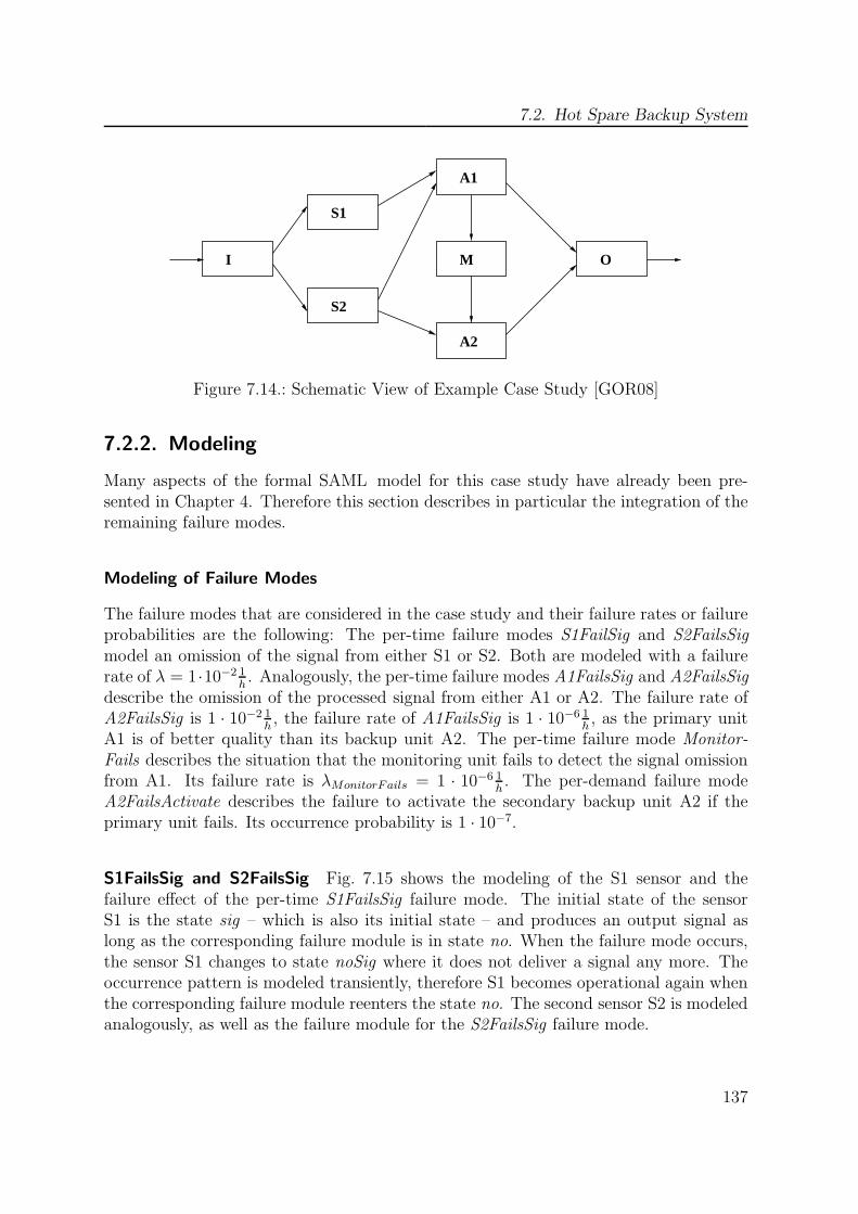
7.2. Hot Spare Backup System
M
S1
A1
O
A2
S2
I
Figure 7.14.: Schematic View of Example Case Study [GOR08]
7.2.2. Modeling
Many aspects of the formal SAML model for this case study have already been pre-sented in Chapter 4. Therefore this section describes in particular the integration of theremaining failure modes.
Modeling of Failure Modes
The failure modes that are considered in the case study and their failure rates or failureprobabilities are the following: The per-time failure modes S1FailSig and S2FailsSigmodel an omission of the signal from either S1 or S2. Both are modeled with a failurerate of λ = 1 ·10−2 1
h. Analogously, the per-time failure modes A1FailsSig and A2FailsSig
describe the omission of the processed signal from either A1 or A2. The failure rate ofA2FailsSig is 1 · 10−2 1
h, the failure rate of A1FailsSig is 1 · 10−6 1
h, as the primary unit
A1 is of better quality than its backup unit A2. The per-time failure mode Monitor-Fails describes the situation that the monitoring unit fails to detect the signal omissionfrom A1. Its failure rate is λMonitorFails = 1 · 10−6 1
h. The per-demand failure mode
A2FailsActivate describes the failure to activate the secondary backup unit A2 if theprimary unit fails. Its occurrence probability is 1 · 10−7.
S1FailsSig and S2FailsSig Fig. 7.15 shows the modeling of the S1 sensor and thefailure effect of the per-time S1FailsSig failure mode. The initial state of the sensorS1 is the state sig – which is also its initial state – and produces an output signal aslong as the corresponding failure module is in state no. When the failure mode occurs,the sensor S1 changes to state noSig where it does not deliver a signal any more. Theoccurrence pattern is modeled transiently, therefore S1 becomes operational again whenthe corresponding failure module reenters the state no. The second sensor S2 is modeledanalogously, as well as the failure module for the S2FailsSig failure mode.
137

7. Case Studies
Module s1 / Sensor1
sig
1
1noSig
s1FailsSig = yes
s1FailsSig 6= yess1FailsSig 6= yes
s1FailsSig = yes
Figure 7.15.: S1FailsSig Failure Effect Modeling
A1FailsSig The modeling of the first arithmetic unit A1 and the failure effects of theper-time failure mode A1FailsSig is shown in Fig. 7.16. A1 is in the initial state startwhen the system is switched on. Afterwards it enters state noSig if the failure modeA1FailsSig occurs or the state Sig if no failure mode occurs. From any of these states itcan be switched off by the monitoring unit. This is normally done if the monitor detectsa signal omission of A1. Once A1 is switched off, it is not possible to become operationalagain.
noSig
Module arith1 / arith1
start offsig
1
¬sigA1
Monitor = degraded
1
1true
¬sigA1
sigA1
sigA1
Monitor = degraded
a1FailsSig 6= yes
∧a1FailsSig 6= yes
∨a1FailsSig = yes
a1FailsSig = yes
∧a1FailsSig 6= yes
∨a1Fails1Sig = yes
Figure 7.16.: A1 with A1FailsSig Failure Effect Modeling
138
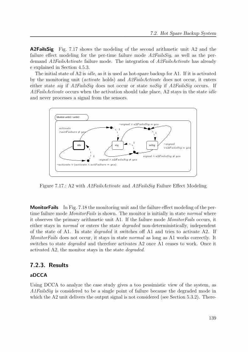
7.2. Hot Spare Backup System
A2FailsSig Fig. 7.17 shows the modeling of the second arithmetic unit A2 and thefailure effect modeling for the per-time failure mode A2FailsSig, as well as the per-demand A2FailsActivate failure mode. The integration of A2FailsActivate has alreadye explained in Section 4.5.3.
The initial state of A2 is idle, as it is used as hot-spare backup for A1. If it is activatedby the monitoring unit (activate holds) and A2FailsActivate does not occur, it enterseither state sig if A2FailsSig does not occur or state noSig if A2FailsSig occurs. IfA2FailsActivate occurs when the activation should take place, A2 stays in the state idleand never processes a signal from the sensors.
Module arith2 / arith2
idle noSig
1
1
¬signal1
sig∨a2FailsSig = yes
1
¬signal ∨ a2FailsSig = yes
activate
¬activate ∨ (activate ∧ actFailure = yes)
signal ∧ a2FailsSig 6= yes
signal ∧ a2FailsSig 6= yes
∧actFailure 6= yes
Figure 7.17.: A2 with A2FailsActivate and A2FailsSig Failure Effect Modeling
MonitorFails In Fig. 7.18 the monitoring unit and the failure effect modeling of the per-time failure mode MonitorFails is shown. The monitor is initially in state normal whereit observes the primary arithmetic unit A1. If the failure mode MonitorFails occurs, iteither stays in normal or enters the state degraded non-deterministically, independentof the state of A1. In state degraded it switches off A1 and tries to activate A2. IfMonitorFails does not occur, it stays in state normal as long as A1 works correctly. Itswitches to state degraded and therefore activates A2 once A1 ceases to work. Once itactivated A2, the monitor stays in the state degraded.
7.2.3. Results
aDCCA
Using DCCA to analyze the case study gives a too pessimistic view of the system, asA1FailsSig is considered to be a single point of failure because the degraded mode inwhich the A2 unit delivers the output signal is not considered (see Section 5.3.2). There-
139
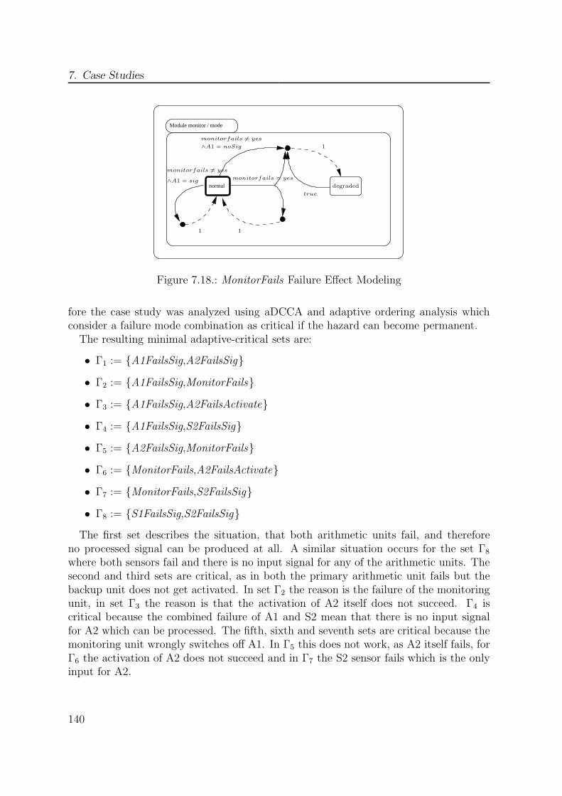
7. Case Studies
Module monitor / mode
normal
1
degraded
1
monitorfails = yes
∧A1 = noSig
∧A1 = sig
1
true
monitorfails 6= yes
monitorfails 6= yes
Figure 7.18.: MonitorFails Failure Effect Modeling
fore the case study was analyzed using aDCCA and adaptive ordering analysis whichconsider a failure mode combination as critical if the hazard can become permanent.The resulting minimal adaptive-critical sets are:
• Γ1 := {A1FailsSig,A2FailsSig}
• Γ2 := {A1FailsSig,MonitorFails}
• Γ3 := {A1FailsSig,A2FailsActivate}
• Γ4 := {A1FailsSig,S2FailsSig}
• Γ5 := {A2FailsSig,MonitorFails}
• Γ6 := {MonitorFails,A2FailsActivate}
• Γ7 := {MonitorFails,S2FailsSig}
• Γ8 := {S1FailsSig,S2FailsSig}
The first set describes the situation, that both arithmetic units fail, and thereforeno processed signal can be produced at all. A similar situation occurs for the set Γ8
where both sensors fail and there is no input signal for any of the arithmetic units. Thesecond and third sets are critical, as in both the primary arithmetic unit fails but thebackup unit does not get activated. In set Γ2 the reason is the failure of the monitoringunit, in set Γ3 the reason is that the activation of A2 itself does not succeed. Γ4 iscritical because the combined failure of A1 and S2 mean that there is no input signalfor A2 which can be processed. The fifth, sixth and seventh sets are critical because themonitoring unit wrongly switches off A1. In Γ5 this does not work, as A2 itself fails, forΓ6 the activation of A2 does not succeed and in Γ7 the S2 sensor fails which is the onlyinput for A2.
140

7.2. Hot Spare Backup System
Deductive Ordering Analysis
Using these eight minimal adaptive-critical sets, adaptive deductive temporal orderinganalysis proves the following adaptive temporal ordering relations:
• MonitorFails�Γ2A1FailsSig
• A1FailsSig≺Γ3A2FailsActivate
• MonitorFails≺Γ6A2FailsActivate
If the monitoring unit fails before or at the same time as the first arithmetic unitfails, it cannot switch to A2 and therefore the hazard occurs. If the monitoring failsafter A1, it can detect the failure of A1 and activate the backup unit. The other twominimal adaptive-critical sets show that A2FailsActivate is only critical if it occurs aftereither A1FailsSig or MonitorFails. The reason for this is that it is a per-demand failuremode which is triggered by the monitor, either by a detected failure of A1 or by amalfunctioning of the monitor. So for Γ3 the critical situation arises just when themonitor detected the malfunctioning of A1, but the activation of A2 does not succeed.For Γ6 the critical situation arises when the monitor wrongly switches off A1 and thenthe activation of A2 does not succeed.The complete analysis time to compute all the adaptive minimal critical sets and
the adaptive temporal ordering relations required 10.114s on a 8 core 2.66 Ghz Xeoncomputer with 16G RAM with NuSMV model-checker version 2.5.
pDCCA
As the case study is a reactive system, bounded pDCCA was conducted using the PRISMmodel-checker version 3.3. Using a sparse matrix representation and a mission time of10h with a temporal resolution of ∆t = 10ms, the full analysis required 3m and 36.7s.The computed maximal probability that the systems fails to deliver an output signalwithin 10h is
Pmax=?[trueU≤3.600.000(observerSig = hazard)] = 9.1490 · 10−7
Advantages over existing methods If a quantitative method based on the a-posteriori analysis of the qualitative results like FTA is used, the estimation of theactual hazard probability is either very pessimistic (if the dependency of the orderingis not considered) or it can get very complex. To increase the accuracy of the analysis,the system model must be analyzed further and the dependencies of the effects of thevarious failure modes must be explored (the model is based on finite state machines andtime passes if a state changes which can then be detected in the next time step).The adaptive deductive ordering analysis clearly showed that the failure modes of this
system are not stochastically independent. Therefore as many of the orderings of the
141
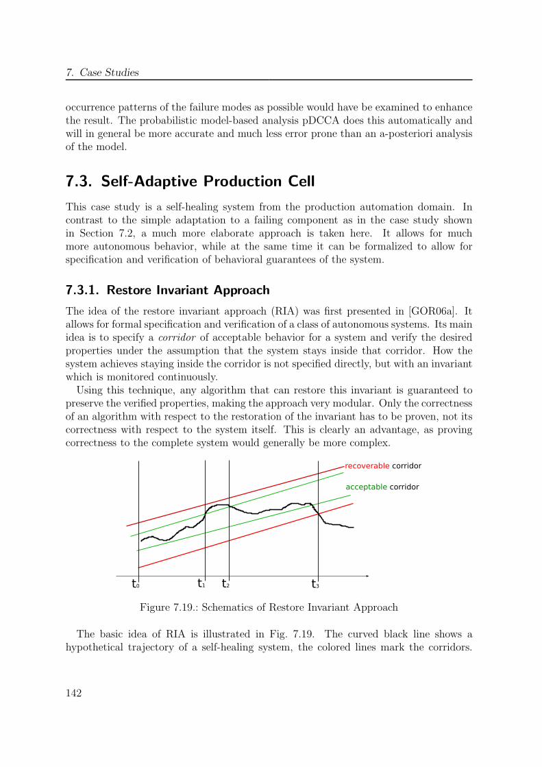
7. Case Studies
occurrence patterns of the failure modes as possible would have be examined to enhancethe result. The probabilistic model-based analysis pDCCA does this automatically andwill in general be more accurate and much less error prone than an a-posteriori analysisof the model.
7.3. Self-Adaptive Production Cell
This case study is a self-healing system from the production automation domain. Incontrast to the simple adaptation to a failing component as in the case study shownin Section 7.2, a much more elaborate approach is taken here. It allows for muchmore autonomous behavior, while at the same time it can be formalized to allow forspecification and verification of behavioral guarantees of the system.
7.3.1. Restore Invariant Approach
The idea of the restore invariant approach (RIA) was first presented in [GOR06a]. Itallows for formal specification and verification of a class of autonomous systems. Its mainidea is to specify a corridor of acceptable behavior for a system and verify the desiredproperties under the assumption that the system stays inside that corridor. How thesystem achieves staying inside the corridor is not specified directly, but with an invariantwhich is monitored continuously.Using this technique, any algorithm that can restore this invariant is guaranteed to
preserve the verified properties, making the approach very modular. Only the correctnessof an algorithm with respect to the restoration of the invariant has to be proven, not itscorrectness with respect to the system itself. This is clearly an advantage, as provingcorrectness to the complete system would generally be more complex.
t0 t1 t2 t3
recoverable corridor
acceptable corridor
Figure 7.19.: Schematics of Restore Invariant Approach
The basic idea of RIA is illustrated in Fig. 7.19. The curved black line shows ahypothetical trajectory of a self-healing system, the colored lines mark the corridors.
142

7.3. Self-Adaptive Production Cell
This is of course not a spatial view of the system, but an abstract view of the states ofthe system states and its behavioral corridor.From the start at t0 to time t1 the system stays in the acceptable corridor (green), the
invariant holds and the system fulfills its desired properties. At t1 the invariant is vio-lated, but the system stays in its recoverable corridor (red) and enters its reconfigurationstate. The adaptation algorithm restores the invariant at t2 and the system stays in theacceptable corridor until t3 when the system leaves its recoverable corridor and a returnto acceptable operation is no more possible.The concept of RIA modeling is rather general: The crucial point is that the adapta-
tion mechanism must be able to decide whether an invariants holds and to restore it ifnot. Such a mechanism can be organized in different ways. For example it can be globalor local and centralized or distributed. Which realization is adequate depends on thetype of model that is considered and also on the available techniques for analysis andverification.The formal RIA modeling presented here considers a system consisting of agents,
each with a set of capabilities. The goal to be fulfilled requires a certain sequence ofapplication of these capabilities. The invariant holds if all required capabilities arepresent and can be used in the correct order. In this situation, all the agents areconfigured to use one of their capabilities to reach the specific goal. If any agent loses itsassigned capability, the invariant may be violated. As long as each required capabilityis present, the invariant can be restored by changing the assignments of the agents inorder to achieve a valid configuration. This describes the recoverable corridor describedabove. Such an adaptation mechanism corresponds to the definition of self-healing asformalized by Seebach et al. in [SOR07]:
“[a system is called] self-healing for a given set C of capabilities and a goalG, if after failure/loss of any capability c ∈ C, then it will eventually cometo [. . .] [an assignment of capabilities] in which G will be achieved again (aslong as this is theoretically possible).”
For modeling in SAML and for formal safety analysis, the possible forms of detection ofinvariant violation and its restoration have to be restricted. The invariant is describedas a Boolean predicate and the restoration mechanism is specified via temporal logicassertions. This will be described in detail in Section 7.3.3.
7.3.2. Description of the Case Study
The modeling approach is illustrated by applying it to a case study from productionautomation. It consists of three robots, which are connected with autonomous trans-portation units. The production cell is self-healing in case of failures of the tools of therobots. This is the reference case study of the SAVE-ORCA project within the prior-ity research program 1183 “Organic Computing” of the German Research Foundation(DFG) and was introduced in [GOR06a] from where the description is adapted:
143

7. Case Studies
Every robot has three capabilities: drill a hole in a workpiece (D), insert a screwinto a drilled hole (I) and tighten an inserted screw (T). These capabilities are executedwith exactly one of the three different tools available for each robot. Every workpiecemust be processed by all three tools in the given order (Drill, Insert, Tighten = DIT).Workpieces are transported from and to the robots by autonomous carts. Changing thetool of a robot is assumed to require some time, therefore the standard configurationof the system is to distribute the capabilities between the three robots and to have thecarts transfer workpieces accordingly.Generally, a valid configuration could be the assignment of multiple capabilities to
one robot. This is not considered here for the reason described above. Therefore aconfiguration of the cell consists of assigning one capability to each robot and assigningautonomous transportation units the task to bring processed workpieces from one robotto the next one in correct processing order, as shown in Fig. 7.20.
Figure 7.20.: Configuration of Robot Cell [SOR07]
If one or more tools break, the current configuration allows no more correct DITprocessing of the incoming workpieces. Such a disturbance is shown in Fig. 7.21(a) inwhich the drill of one robot broke and DIT processing is not possible any more, as noother robot is configured to drill. A more traditional production cell would probablystop working and wait for maintenance.However in this situation, it is obvious that the robots would still be able to achieve
the overall goal, as in theory all three tools are available. The robot with the broken tooljust has to switch to another tool. So it should be possible for a self-healing system todetect this situation and reconfigure itself. This works of course only if in addition to therobot with the broken tool, at least one of the other robots also switches its capability.
144

7.3. Self-Adaptive Production Cell
(a) Temporary Hazard due to Broken Drill (b) Reconfigured Robot Cell
Figure 7.21.: Invariant Violation and Restoration [SOR07]
One possible reconfiguration outcome is shown in Fig. 7.21(b). Now the left robotdrills, the right robot tightens the screws and the middle robot is left unchanged. Forthis error resolution, not only the assignment of the tasks to the robots must be changed,but also the routes of the carts and the routing of the incoming and outgoing workpieces.If only the tools were switched, the processing of all tasks would be possible, but not inthe correct order.
This example only shows one reconfiguration for one error. Additional reconfigurationscan take place if other tools break. Of course there is an end to the possibility of adaptionwhen the necessary tools are no more available, i.e. when all drills break or when onerobot has no more intact tools at all.In summary, this self-healing system tries to preserve its functionality as long as
possible even if some of the tools break. This is achieved by reconfiguration and worksas long as there is enough internal redundancy in the system.
7.3.3. Modeling
The purpose of the modeling of this case study was to validate the feasibility of a formalsafety-analysis of a self-healing system and to illustrate the application of the restore-invariant approach. Currently it is not possible to use the restore invariant approach ina probabilistic model, therefore the modeling presented here is purely qualitative. Theexact reason for this will be explained in more detail in the last part of this section. Thismeans that the different possible successor states are chosen in a purely non-deterministicway. The basis for the formal modeling presented here was introduced in [GOR06a], itssafety analysis was introduced in [GOR06b].
145
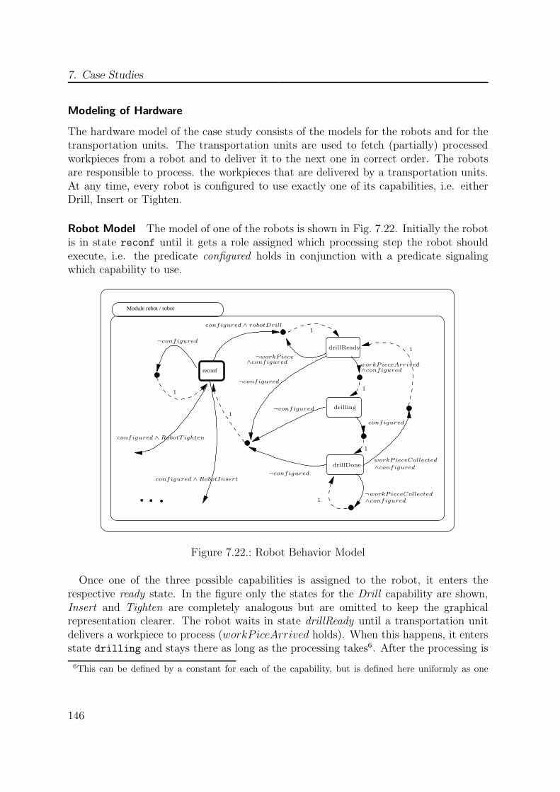
7. Case Studies
Modeling of Hardware
The hardware model of the case study consists of the models for the robots and for thetransportation units. The transportation units are used to fetch (partially) processedworkpieces from a robot and to deliver it to the next one in correct order. The robotsare responsible to process. the workpieces that are delivered by a transportation units.At any time, every robot is configured to use exactly one of its capabilities, i.e. eitherDrill, Insert or Tighten.
Robot Model The model of one of the robots is shown in Fig. 7.22. Initially the robotis in state reconf until it gets a role assigned which processing step the robot shouldexecute, i.e. the predicate configured holds in conjunction with a predicate signalingwhich capability to use.
reconf
Module robot / robot
1
¬configured
1
¬configured
1
configured ∧ robotDrill
drillReady
drillDone
drilling
¬workPiece
1
1
1
1
¬workPieceCollected
configured ∧ RobotInsert
configured ∧ RobotTighten
workPieceCollected
¬configured
configured
∧configured
∧configured
∧configured
∧configured
¬configured
workPieceArrived
Figure 7.22.: Robot Behavior Model
Once one of the three possible capabilities is assigned to the robot, it enters therespective ready state. In the figure only the states for the Drill capability are shown,Insert and Tighten are completely analogous but are omitted to keep the graphicalrepresentation clearer. The robot waits in state drillReady until a transportation unitdelivers a workpiece to process (workP iceArrived holds). When this happens, it entersstate drilling and stays there as long as the processing takes6. After the processing is
6This can be defined by a constant for each of the capability, but is defined here uniformly as one
146
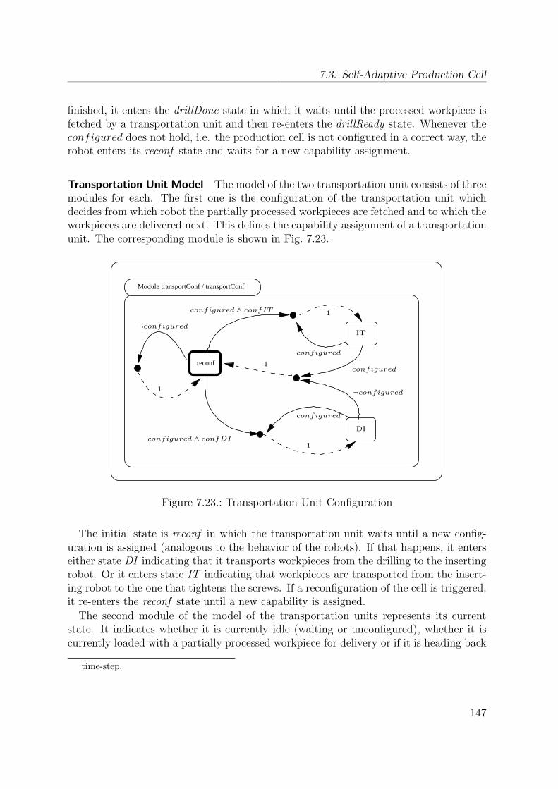
7.3. Self-Adaptive Production Cell
finished, it enters the drillDone state in which it waits until the processed workpiece isfetched by a transportation unit and then re-enters the drillReady state. Whenever theconfigured does not hold, i.e. the production cell is not configured in a correct way, therobot enters its reconf state and waits for a new capability assignment.
Transportation Unit Model The model of the two transportation unit consists of threemodules for each. The first one is the configuration of the transportation unit whichdecides from which robot the partially processed workpieces are fetched and to which theworkpieces are delivered next. This defines the capability assignment of a transportationunit. The corresponding module is shown in Fig. 7.23.
reconf
Module transportConf / transportConf
DI
IT
1
1
¬configured
1
1
configured
configured
¬configured
¬configured
configured ∧ confDI
configured ∧ confIT
Figure 7.23.: Transportation Unit Configuration
The initial state is reconf in which the transportation unit waits until a new config-uration is assigned (analogous to the behavior of the robots). If that happens, it enterseither state DI indicating that it transports workpieces from the drilling to the insertingrobot. Or it enters state IT indicating that workpieces are transported from the insert-ing robot to the one that tightens the screws. If a reconfiguration of the cell is triggered,it re-enters the reconf state until a new capability is assigned.
The second module of the model of the transportation units represents its currentstate. It indicates whether it is currently idle (waiting or unconfigured), whether it iscurrently loaded with a partially processed workpiece for delivery or if it is heading back
time-step.
147
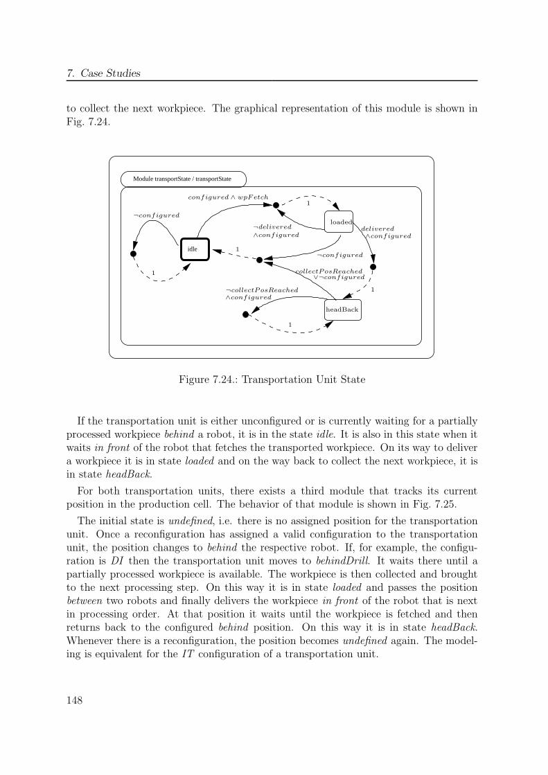
7. Case Studies
to collect the next workpiece. The graphical representation of this module is shown inFig. 7.24.
idle
Module transportState / transportState
1
¬configured
1
1configured ∧ wpFetch
headBack
loaded
1
delivered
1
collectPosReached
¬delivered
∧configured
¬configured
∨¬configured
∧configured
¬collectPosReached∧configured
Figure 7.24.: Transportation Unit State
If the transportation unit is either unconfigured or is currently waiting for a partiallyprocessed workpiece behind a robot, it is in the state idle. It is also in this state when itwaits in front of the robot that fetches the transported workpiece. On its way to delivera workpiece it is in state loaded and on the way back to collect the next workpiece, it isin state headBack.
For both transportation units, there exists a third module that tracks its currentposition in the production cell. The behavior of that module is shown in Fig. 7.25.
The initial state is undefined, i.e. there is no assigned position for the transportationunit. Once a reconfiguration has assigned a valid configuration to the transportationunit, the position changes to behind the respective robot. If, for example, the configu-ration is DI then the transportation unit moves to behindDrill. It waits there until apartially processed workpiece is available. The workpiece is then collected and broughtto the next processing step. On this way it is in state loaded and passes the positionbetween two robots and finally delivers the workpiece in front of the robot that is nextin processing order. At that position it waits until the workpiece is fetched and thenreturns back to the configured behind position. On this way it is in state headBack.Whenever there is a reconfiguration, the position becomes undefined again. The model-ing is equivalent for the IT configuration of a transportation unit.
148

7.3. Self-Adaptive Production Cell
undefined
Module TransportPos / transportPos
1
¬configured
1
behindDrill
betweenDI
1
configured ∧ DrillInsert
1
1
configured ∧ InsertTighten
¬configured
¬configured
¬configured
inFrontInsert
∧configured
∧configured
∧configured
transportState = loaded
transportState = loaded
transportState = headBack
transportState 6= loaded
∧configured
transportState = headBack∧configured
1
1
Figure 7.25.: Transportation Unit Position
Modeling of Physical Behavior
The physical behavior model in the case study contains primarily the processing of theworkpieces. Each of the workpieces consists of two modules: one tracks the currentposition of the workpiece, the other tracks its current processing state.
Workpiece Model The position of the workpiece is tracked throughout the productioncell. At the beginning it is located outside of the cell, in the storage. For each robotand tool, it then passes from the in front position to the in position, onto the afterposition. This can be seen in Fig. 7.26 for the Drill capability.The workpiece stays in front of one of the robots until it is ready. When this happens,
its position changes to in, meaning it is currently processed. This position is changedas soon as the robot signals the completion of the task, causing the position of theworkpiece to change to after, where it stays until one of the transportation units collectsit for delivery to the next robot. If both transportation units arrive to collect theworkpiece, the production would come to a standstill. This should of course preventedby a correct capability assignment.When the workpiece is located on one of the transportation units, it gets delivered to
either the drilling or inserting robot, where its position changes analogously as explainedabove for the Drill capability. After the last processing step (Tighten capability), itsposition changes to behindCell (not shown in the figure), indicating the completion ofthe processing.The processing state of the workpiece is described via three state variables: one to
149
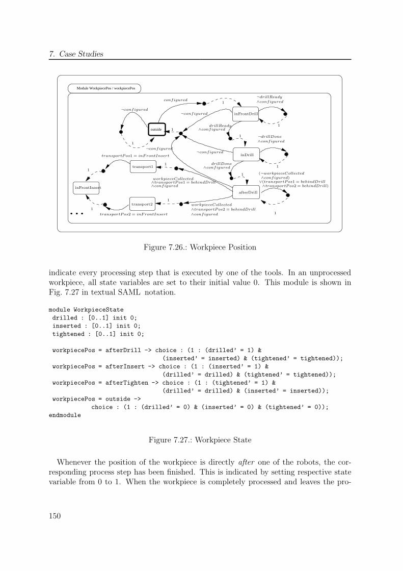
7. Case Studies
outside
Module WorkpiecePos / workpiecePos
1
¬configured
1
inFrontDrill
configured¬drillReady
¬drillDone
workpieceCollected
∧transportPos2 = behindDrill
∧configured
∧configured
inDrill
1
1
¬configured
drillDone∧configured
drillReady∧configured
¬configured
transport1
transport21
1
1
1
1
inFrontInsert
¬configured
1
1
transportPos1 = inFrontInsert
transportPos2 = inFrontInsert ∧configured
∨(transportPos1 = behindDrill
1
afterDrill
(¬workpieceCollected
∧configured)
∧transportPos2 = behindDrill)∧configured∧transportPos1 = behindDrillworkpieceCollected
Figure 7.26.: Workpiece Position
indicate every processing step that is executed by one of the tools. In an unprocessedworkpiece, all state variables are set to their initial value 0. This module is shown inFig. 7.27 in textual SAML notation.
module WorkpieceState
drilled : [0..1] init 0;
inserted : [0..1] init 0;
tightened : [0..1] init 0;
workpiecePos = afterDrill -> choice : (1 : (drilled’ = 1) &
(inserted’ = inserted) & (tightened’ = tightened));
workpiecePos = afterInsert -> choice : (1 : (inserted’ = 1) &
(drilled’ = drilled) & (tightened’ = tightened));
workpiecePos = afterTighten -> choice : (1 : (tightened’ = 1) &
(drilled’ = drilled) & (inserted’ = inserted));
workpiecePos = outside ->
choice : (1 : (drilled’ = 0) & (inserted’ = 0) & (tightened’ = 0));
endmodule
Figure 7.27.: Workpiece State
Whenever the position of the workpiece is directly after one of the robots, the cor-responding process step has been finished. This is indicated by setting respective statevariable from 0 to 1. When the workpiece is completely processed and leaves the pro-
150

7.3. Self-Adaptive Production Cell
duction cell (its position becomes behindCell), all processing steps are deleted again andit is reintroduced into the production cell (the position becomes outside again). Thereason for this is that there is only a finite amount of modules can be specified in aSAML model. With this modeling, the production can continue arbitrary long, as therewill always eventually be unprocessed workpieces available.Based on the described modules, the production cell can fulfill the goal to process
workpieces in DIT order, if a fixed and correct initial assignment of the capabilities isspecified. In such a situation, there would be a continuous processing of workpieces whichafter leaving the cell will be “reset” and reintroduced in the storage. The continuousand correct processing can be verified as shown in [GOR06a].
Modeling of Failure Modes
But of course from the point of safety analysis, more interesting than functional cor-rectness of one specific configuration is its behavior under the occurrence of failures.The failure modes that are modeled in the case study are the loss of capabilities of therobots (i.e. the corresponding tool breaks). To model broken tools in the productioncell, persistent failure modules are used for all tools of all robots. The considered failuremodes are the following:
• R1FailsD : broken drill of robot 1
• R1FailsI : broken insertion mechanism of robot 1
• R1FailsT : broken tightening mechanism of robot 1
• R2FailsD : broken drill of robot 2
• R2FailsI : broken insertion mechanism of robot 2
• R2FailsT : broken tightening mechanism of robot 1
• R3FailsD : broken drill of robot 3
• R3FailsI : broken insertion mechanism of robot 3
• R3FailsT : broken tightening mechanism of robot 1
The most appropriate failure mode modeling in this case study would be a per-demandmodeling, as the abstraction is that the tools are used for exactly one time-step wherethey can get broken. But as the model of the case study is not probabilistic, the dis-crimination between per-time and per-demand is not necessary here and the simpler andless complex per-time failure mode integration was chosen.The integration of the failure modes into the extended system model works as follows:
whenever the tool breaks which belongs to the currently assigned capability, then the
151
7. Case Studies
respective robot enters its reconf state and processes no more workpieces. This meansthat the robot locally detects the occurrence of the failure mode, but not necessarily theglobal invariant violation. The robot waits in that state until it gets a new capabilityassignment from the invariant restoration mechanism. The integration is realized byintroducing new transitions from the working states of a robot to its reconfigurationstate.
Modeling of Software for RIA
After the integration of the failure modes, the mechanism of detection and restorationof the invariant can be specified in the form of the restore invariant approach. The RIAmodeling presented here was first introduced in [GOR06a] and uses Boolean predicatesto monitor the invariant and temporal logic assertions to restore it. Its formalization ispresented in detail here for reasons of clarity, necessary for safety analysis is merely thefact that it exists and works.
For a more compact expression, predicates are introduced which describe the state ofthe robots. The predicates Ra
i with i ∈ {1, 2, 3} and a ∈ {d, i, t} hold if robot i has beenassigned to used the capability a (at most one single capability can be assigned to arobot at a time, i.e. Ra
i →∧
b∈{d,i,t}\a ¬Rbi). This means for example that Rd
2 holds if themodule corresponding to the robot 2 is either in state drillReady, drilling or DrillDone.
The next predicates describe the state of the transportation units. Cxj with j ∈
{1, 2} and x ∈ {it, di} are modeled analogously to the robot predicates and refer tothe capability assignment in the model of the carts. For example, Cdi
1 holds if the cart1 has been assigned to fetch partially processed workpieces from robot with the Drillcapability for further processing of the robot with the Insert capability (analogous to Ra
i
at most one of the possible predicates can hold for each cart).
These predicates form the basis for the formalization of RIA. Using them, a configu-ration of the robots (i.e. each robot has an assigned capability) is defined as shown inEq. (7.4). A configuration of the carts is defined as shown in Eq. (7.5). This means thatrobotConf and carConf hold if neither one of the robot nor one of the cart awaits areconfiguration.
robotConf := (Rd1 ∨ R
i1 ∨ R
t1) ∧ (Rd
2 ∨Ri2 ∨ R
t2) ∧ (Rd
3 ∨Ri3 ∨ R
t3) (7.4)
cartConf := (Cdi1 ∨ C it
1 ) ∧ (Cdi2 ∨ C it
2 ) (7.5)
This does not necessarily specify a configuration in such a way that all required ca-pabilities are available for correct processing. This fact is described with ditCapable
in Eq. (7.6) for a valid robot configuration (not considering any failures) and with
152

7.3. Self-Adaptive Production Cell
cartCapable in Eq. (7.7) for a valid cart configuration.
ditCapable :=∧
a∈{d,i,t}
∨
j∈{1,2,3}
Raj ∧
∧
k∈{1,2,3}\j
¬Rak
(7.6)
cartCapable :=∧
x∈{di,it}
∨
j∈{1,2}
Cxj ∧
∧
k∈{1,2}\j
¬Cxk
(7.7)
For the definition of the invariant, it is necessary to also consider the occurrence ofthe various failure modes. To specify this, the predicates failsai with i ∈ {1, 2, 3} anda ∈ {d, i, t} are used, where failsai holds if the tool a of robot i is broken. For example,if the failure mode R1FailsD occurs and the corresponding failure module is in state yes,then failsd1 holds. Using these, the failure of a single robot j is signaled by ditFailurej(see Eq. (7.8)) which states that a robot has been assigned a capability that it canno longer use because its required tool is broken. Eq. (7.9) defines ditFailure as thedisjunction of the failures of all robots in the cell.
ditFailurej :=∨
a∈{d,i,t}
(Raj ∧ fails
aj ) (7.8)
ditFailure :=∨
i∈{1,2,3}
ditFailurej (7.9)
Therefore the invariant to monitor is the predicate ¬ditFailure which holds if thesystem is in its acceptable corridor. It indicates that there is no robot which cannot useits currently assigned capability. Now, whenever the invariant restoration mechanismdetects that ditFailure holds, it must trigger a reconfiguration and restore the invariant.For proving functional properties and the specification of a correct reconfiguration
mechanism, it must be possible to identify whether the system is still in its recoverablecorridor so that it is theoretically possible to restore the invariant. This is expressedwith the predicate ditPossible. In this modeling, it is defined as the disjunction of theenumeration of all possible valid configurations. The reason for this is the fact thatSAML currently does not support the usage of quantifiers7.The abstract invariant restoration can then be defined using the previous definitions.
It consists of two temporal logic specifications: confDIT Eq. (7.10) and confCorrectEq. (7.11).
confDIT := G ((robotConf ∧ cartConf) → ditCapable ∧ cartCapable) (7.10)
7A possibility for a more general modeling based on the formal RIA approach introduced here, butusing the Alloy constraint solver is described by Gudemann et al. in [GNO+08]
153
7. Case Studies
Here confDIT specifies that every reconfiguration results in a valid configuration ofthe production cell according to the specification. Whenever (G ) the robots and thecarts are configured (robotConf ∧cartConf), then all required capabilities are available,i.e. all required tools for the robots (ditCapable) are available and the routes for thecarts (cartCapable) are set correctly.
confCorrect := G ((endReconf) → X(ditPossible→ ¬ditFailure)) (7.11)
The confCorrect property specifies that whenever a reconfiguration has just beenfinished (endReconf), then in the next time-step (i.e. the first processing step after thereconfiguration) only available capabilities have been assigned (the invariant ¬ditFailureholds) as long as the system is in the recoverable corridor (ditPossible). This meansthat a reconfiguration is always successful as long as a correct reconfiguration is stillpossible despite potential occurrences of single failures. Note, that no proposition aboutthe carts appears in confCorrect as there is no failure mode modeled for them.These LTL formulas are used as assumptions to prove properties of the system. They
are assumed to be true – a correct invariant restoration mechanism exists – and otherproperties (in particular the aDCCA proof obligations) are proven under this assump-tion. This approach forms the basis of the invariant restoration mechanism. To mycurrent knowledge the only tool that supports this directly8 is the Cadence SMV modelchecker. So currently an extended system model of a self-healing system specified usingRIA can only be analyzed with this verification tool. Either by direct specification inits input language or by transforming a system model into it.Now everything required for a detection of a violation of the invariant and the restora-
tion thereof has been defined, with the exception of a model of the actual capabilityassignment. This is conducted by the additional module Control which consists of thestate variable control. Its graphical representation of the module is shown in Fig. 7.28.Its initial value is reconf. From there it enters the state initialize, where it stays
until all three robots and both transportation units are also in their After then, it non-deterministically enters one of the states r1D, r1I and r1T. Each signals which capabilityis assigned to the first robot. This is repeated for the second and third robot (not shownin the figure). After the assignment for the third robot, the control non-deterministicallyenters the states t1DI or t1IT for the assignment of the route for the first transportationunit and after then t2DI or t2IT which assigns the route to the second transportationunit. Finally it enters the state endReconf, signaling the end of the reconfiguration.Then it enters state idle and stays in this state until the predicate ditFailure holds, i.e.a new reconfiguration must be done.The assumption mechanism of the Cadence SMV model checker is used to assume
confDIT and confCorrect for verification of other properties. In effect, these LTLformulas specify that whenever the Control module has just completed an assignment
8via the construct using confDIT, confCorrect prove ...
154
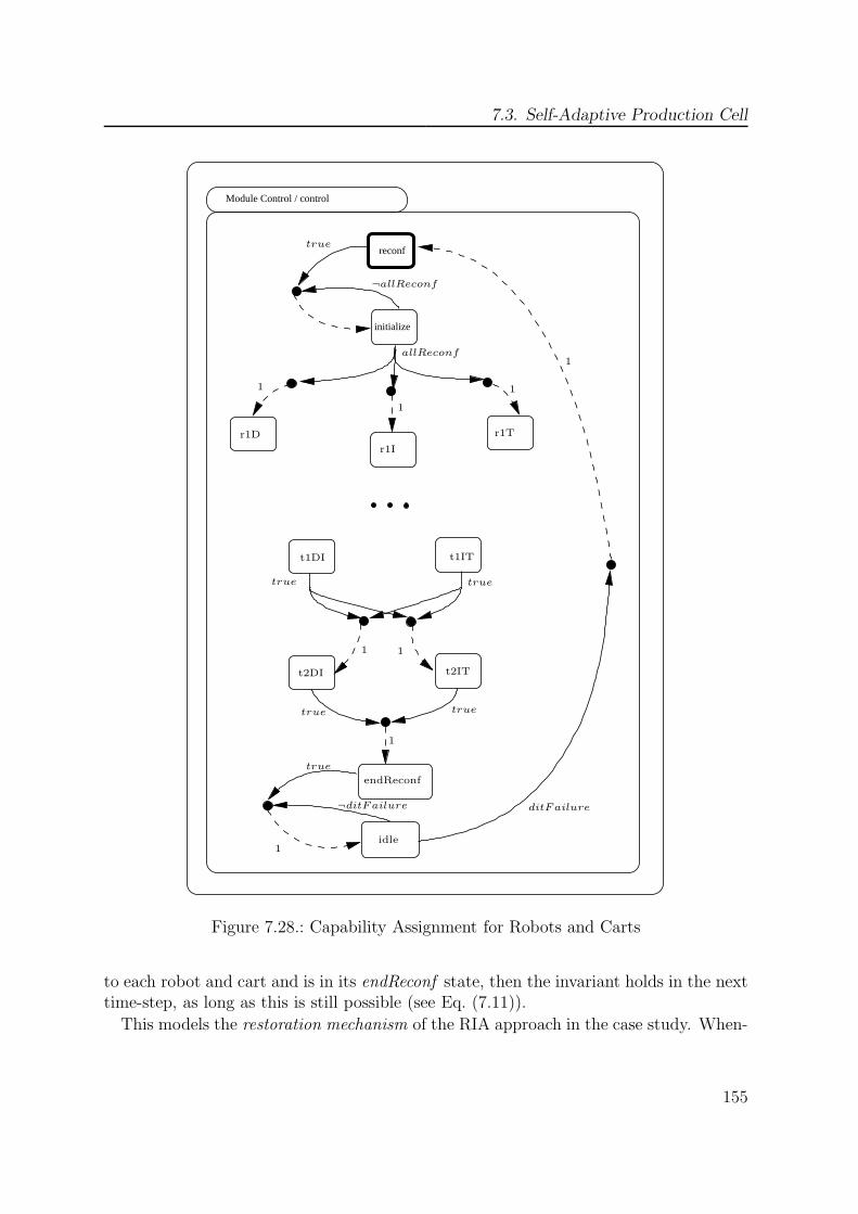
7.3. Self-Adaptive Production Cell
Module Control / control
reconf
initialize
truetrue
1 1
1
r1D
r1I
r1T
allReconf
endReconf
1
truetrue
true
ditFailure
1
1
true
¬ditFailure
11
¬allReconf
idle
t1DI t1IT
t2DI t2IT
Figure 7.28.: Capability Assignment for Robots and Carts
to each robot and cart and is in its endReconf state, then the invariant holds in the nexttime-step, as long as this is still possible (see Eq. (7.11)).
This models the restoration mechanism of the RIA approach in the case study. When-
155

7. Case Studies
ever a reconfiguration is triggered, the configuration by the control module will be non-deterministic, but will result in a valid one. Practically this limits the verification oftemporal logic properties to only those traces where valid configurations are reached.Now it also becomes clear why this is difficult for quantitative analysis. One problem is
that the currently available probabilistic model checkers do not support the assumptionmechanism. This problem could perhaps be solved by transforming the LTL assump-tions to an automaton. Nevertheless, the effect on the resulting probability space isunclear which makes the interpretation of the analysis results very difficult. In effectthe RIA approach limits the traces on which the properties are verified to those wherethe restoration works correctly. This means that the computed probabilities would al-ways have to be considered in relation to the probability that the restoration does notsucceed. Nevertheless, currently it is not possible to compute this, as there are manydifferent (possibly infinitely many) adversaries possible that do not restore the invari-ant correctly, but the verification allows only the computation of the maximizing orminimizing adversary.A possible solution would be the specification of one explicit reconfiguration mecha-
nism. But this would bypass RIA itself and be much less flexible. Quantitative model-based safety analysis of self-healing systems with such a degree of autonomy must there-fore still be considered an open research question.
7.3.4. Results
aDCCA
The analysis to compute all adaptive minimal critical sets on a 2.6Ghz Xeon CPU with16G RAM required 262.76s. In total 262 proof obligations had to be checked for completeaDCCA. This resulted in the following adaptive minimal critical sets:
• Γ1 := {R1FailsD,R1FailsI,R1FailsT}
• Γ2 := {R2FailsD,R2FailsI,R2FailsT}
• Γ3 := {R3FailsD,R3FailsI,R3FailsT}
• Γ4 := {R1FailsD,R2FailsD,R3FailsD}
• Γ5 := {R1FailsI,R2FailsI,R3FailsI }
• Γ6 := {R1FailsT,R2FailsT,R3FailsT}
• Γ7 := {R1FailsD,R1FailsI,R2FailsD,R2FailsI }
• Γ8 := {R1FailsD,R1FailsI,R3FailsD,R3FailsI }
• Γ9 := {R3FailsD,R3FailsI,R2FailsD,R2FailsI }
156
7.3. Self-Adaptive Production Cell
• Γ10 := {R1FailsD,R1FailsT,R2FailsD,R2FailsT}
• Γ11 := {R1FailsD,R1FailsT,R3FailsD,R3FailsT}
• Γ12 := {R3FailsD,R3FailsT,R2FailsD,R2FailsT}
• Γ13 := {R1FailsI,R1FailsT,R2FailsI,R2FailsT}
• Γ14 := {R1FailsI,R1FailsT,R3FailsI,R3FailsT}
• Γ15 := {R3FailsI,R3FailsT,R2FailsI,R2FailsT}
The result of the analysis are 15 minimal adaptive-critical sets, 6 of size 3 and 9 ofsize 4. The minimal adaptive-critical sets Γ1, Γ2 and Γ3 describe the situation that oneof the robots loses all its capabilities. This makes the production impossible, as in thevariant of the case study presented here the robots cannot be configured to fulfill twocapabilities at the same time. Nevertheless, this could be realized as a degraded modein a more complex version of the case study.
The minimal adaptive-critical sets Γ4, Γ5 and Γ6 describe the situation, that one ofthe capabilities is completely unavailable. As every capability is required, this situationis critical for the production cell.
The remaining 9 minimal adaptive-critical sets of size 4 (Γ7 to Γ15) describe a differentsituation: each robot still has a capability left and overall all capabilities are available.Still it is no longer possible to configure the production cell correctly, because two of therobots have only the same single capability left and therefore the third one would haveto be configured to use more than one capability at a time.
Ordering Analysis
An adaptive ordering on the adaptive-critical sets could not be found. The reason forthis is that both the initial capability allocation as well as the resolving of the temporaryhazard is done autonomously by the invariant restoration. This means that there is nofixed sequence of allocation of capabilities and therefore any sequence of failure modeoccurrence can be problematic.
Advantages over existing methods This case study clearly shows the advantage ofusing aDCCA for an adaptive system. In general. it is difficult to know beforehand howlong the reconfiguration needs and how many broken tools can be tolerated. Using therestore invariant approach is a convenient abstraction which allows for the verificationand safety analysis of a self-healing system, independent of the concrete implementationof the reconfiguration algorithm. Any algorithm that manages to restore the invariantas long as possible, retains the properties that are verified with RIA.
157

7. Case Studies
7.4. Related Work
The first case study in Section 7.2 has been introduced by Walker et al. [WBP07], whereit is analyzed using an algebraic approach. A comparison of the analysis method usedby Walker et al. in [WBP07] and Walker and Papadopoulos in [WP07] is discussed inSection 5.4.
The autonomous production cell and the restore invariant approach were introducedin [GOR06a]. The approach has been extended in [GNO+08] to cover more generalresource-flow systems modeled in the Organic Design Pattern (ODP) developed by See-bach et al. [SOR07]. In the ODP, an UML model is extended with OCL constraints whichare used to describe the invariant that must be restored. A method to check whetherthis invariant is violated using constraint solvers like Alloy was developed by Gudemannet al. in [GNO+08] and based on KodKod by Nafz et al. in [NOS+09]. These approachesare still limited to a fixed number of robots, workpieces and autonomous transportationunits. The newest extension of the RIA formalization approach described by Nafz etal. in [NSS+10] uses interactive theorem proving and modularization which allows anunlimited number of agents in such a system. The functional properties of the systemare formulated in interval temporal logic (ITL) (e.g. see Cau [CMZ02]) which is for-malized in KIV as described by Balser et al. [BBR08]. This is an interesting approachwhich significantly extends the basic RIA modeling presented in this chapter. On theother hand, this approach is not well suited for safety analysis, as this is inherentlystate-based quickly becomes problematic for interactive theorem proving. In addition,aDCCA (and of course pDCCA) is not directly expressible in ITL. It seems much moresuited to verify functional properties of larger self-healing systems that can be modeledin the ODP framework than for safety analysis.
The radio based railway crossing was analyzed by Reif et al. using formal faulttree analysis and interactive theorem proving in [RST00] and Thums and Schellhornin [TS02]. The first use of failure injection, model-based safety analysis and model-checking for the analysis of the case study was presented by Ortmeier et al. in [ORS05].Both these analyses where purely qualitative and did not allow for the computation ofhazard probabilities. For the estimation of hazard probabilities, the fault-tree formulawas used which is very coarse and assumes stochastic independence. A distinction be-tween per-time and per-demand failure modes is not possible in any of these approaches.Ortmeier et al. introduced safety optimization in [OSR04]. In this approach an addi-tional safety margin and the allowed speed for the train were used as parameters of anadditional model of stochastic behavior based on distribution functions. This model con-sisted of the opposing goal to minimize the time-delay at the crossing and to minimizethe hazard probability. These goals are weighted according to their projected costs andthe resulting scalar function can be optimized using mathematical optimization tech-niques. A more detailed description can be found in Ortmeier’s dissertation [Ort06].This basic approach can be extended using the quantitative model-based analysis pD-CCA as objective function for optimization as described in [GO11a] which gives more
158
7.4. Related Work
accurate results than the a-posteriori estimations for the hazard probabilities used be-fore. Using multi-objective optimization also allows for computing non-convex Paretosets (optimal compromises). A serious limitation of the previous scalarization approachwas that only convex Pareto sets could be found.
Summary
This chapter presented modeling and model-based safety analysis of three different casestudies. The case studies were selected to show how different types of systems can bemodeled and how different concrete analyses work. It also showed the current limitsof the approach. Quantitative analysis of a more autonomous case study is currentlynot possible. On the other hand, the safety analyses of each case study were beyondthe current state of the art and more accurate than previously possible. The majorachievement is the successful quantitative model-based safety analysis of the larger casestudy of the railroad crossing. It clearly shows that the full approach – in particular theresource-intensive probabilistic analysis – is definitely applicable to real-world systems.
159


8. Conclusion And Outlook
The true logic of this world is in the calculus ofprobabilities.
(James Clerk Maxwell)
This dissertation introduced new formal, model-based qualitative and quantitativesafety analysis methods which advance the current state of the art. The foundation forthese is the new formal modeling framework SAML which allows convenient specificationof formal models of safety-critical systems for accurate qualitative and quantitative for-mal safety analysis. Modeling guidelines showed how accurate models of different failuremodes and realistic physical behavior models can be expressed in SAML. Semanticallywell-founded model transformations allow for using the most appropriate and efficientverification tools. Several case studies showed the benefit and efficiency of the approachand illustrated the application of formal modeling and safety analysis.
161
8. Conclusion And Outlook
8.1. Summary and Conclusion
8.1.1. Summary
SAML
The developed SAML modeling framework allows for convenient expression of formalmodels for safety analysis. With SAML, it is possible to combine non-deterministic, qual-itative and probabilistic, quantitative behavior in a single system model. This allows foraccurate specification of different kinds of failure modes and of the behavior of a system’sphysical environment. SAML is designed as a tool-independent language. Semanticallywell-founded model transformations convert SAML models fora specific analyses withappropriate verification tools . The model transformations are proven to be semanticallysound and preserve the model semantics. This tool-independent approach makes anyadvancement of the verification tools directly usable for safety analysis.Note that one example of this effect is the support for stochastic hypothesis testing
which allows computation of confidence intervals even in the case of models that aretoo large for full model checking [You05]. This feature is introduced in version 4.0 ofthe PRISM model checker, but was not available in version 3.3 that was available whenpDCCA was originally developed. Now stochastic hypothesis testing can be used for theanalysis of SAML models without any change to the model transformations.
Modeling and Safety Analysis Methods
Different new analysis techniques have been developed for accurate formal safety analysisof SAML models. These extend the analyzable class of systems, augment the qualitativesafety analysis results and allow for a combined qualitative and quantitative, model-based safety analysis of extended SAML system models.The basis for accurate safety analysis are the modeling methods for different types
of failure modes. They allow for a sound combination of per-time and per-demandfailure mode modeling in the same model which was not possible in previous approaches.Probabilistic modeling also allows for a more accurate modeling of the behavior of thephysical environment of a system resulting in more precise safety analysis results.Critical combinations of failure modes, e.g. computed with the previous analysis
method DCCA, can be further analyzed using deductive ordering analysis. It allows fora more precise qualitative safety analysis than before. Its results can be used to augmentthe effect of the implementation of risk-reducing measures by identifying the failuremodes where a reduction of risk is most beneficial. Using deductive ordering analysisalso allows for an automatic deduction of several dynamic fault tree gates directly froma system model.Probabilistic DCCA enhances the previous quantitative safety analysis results which
were based on a-posteriori analysis of critical failure mode combinations. Quantita-tive safety analysis with pDCCA allows for accurate computation of hazard occurrence
162
8.1. Summary and Conclusion
probabilities directly on the system model. It does not rely on the assumption of stochas-tic independence and allows for a combined analysis of per-time and per-demand failuremodes in a single model. This was not considered in any existing failure-injection, model-based safety analysis approach. It is much more accurate than previous a-posterioriestimations, in particular by automatically considering all system inherent logical andstochastic dependencies which were very hard or even impossible to consider in previousapproaches.Adaptive DCCA and adaptive deductive ordering analysis are an extension of the
qualitative safety analysis methods to self-healing systems with a certain degree of au-tonomy. The restore invariant approach was developed as a very general way of formallyspecifying self-healing systems. It allows a very flexible way to define self-healing be-havior. Based on RIA, qualitative properties of self-healing systems can be verified withaDCCA, which was not so generally possible before. Quantitative safety analysis of self-healing systems is possible if a modeling approach based on an observer is used insteadwhich seems to be possible for a large class of systems.The applicability of the presented modeling and safety analysis techniques to practical
examples has been demonstrated with several case studies with sizes of more than 107
states. It has been shown that these methods allow a much more accurate assessmentof the safety of a system than was possible before. One key aspect is that both quali-tative and quantitative analyses are conducted on an equivalent model. This raises theconfidence in the computed results, as it is guaranteed that they are “compatible” toeach other. The effort needed for modeling and analysis has also proven to be accept-able. Due to the tool-independence, the analysis effort will be reduced further by thecontinuing advancement and increasing efficiency of verification tools.
8.1.2. Conclusion
In conclusion, the greatest benefit of the results of this dissertation is the possibilityof conducting probabilistic safety analysis directly on extended system models whileproviding means of combining per-time and per-demand failure modes in the analysis.This was not possible before and marks an important step forward in the state of theart. The second main benefit is bridging the gap between qualitative and quantitativesafety analysis achieved by the definition of SAML and the semantically well-foundedtransformations of SAML models into the input specification of different verificationtools. This increases confidence in the results of the safety analyses by assuring thecompatibility of these different views on the properties of a safety-critical system.These techniques could be a great help for the safety engineer in assessing the safety of
a system in the early design phases. Different system variants can be compared, criticalfailure combinations can be identified and risk-reducing measures can be applied. Theeffects can be analyzed by inspecting the computed counterexamples which serve as“witnesses” for properties. They can provide very useful insights into the functioning ofthe system, as Edmund M. Clarke puts it in the Birth of Model-Checking [Cla08]:
163
8. Conclusion And Outlook
“It is impossible to overestimate the importance of the counterexample fea-ture.”
New developments even allow the use of probabilistic analysis to compute the mostprobable counterexamples. Approaches for this are described by Han et al. [HKB09]and Aljazzar et al. [AKLFL10]. This means that risk-reducing measures can be appliedwhere their effect will be most significant. Due to the tool-independence of SAML, thedescribed safety analysis approach benefits directly from such new developments withoutadditional effort.Nevertheless, it is important to note that the results of the safety analyses should be
interpreted by an expert in the field. Formal model-based safety analysis is primarily anextension of existing safety analysis. The subtitle of this dissertation – “Push the safetybutton” – is meant in the following way: using the safety analysis methods presented inthis dissertation, it is possible to support the safety engineer by allowing safety analysisin early design phases of the development process and facilitating accurate comparisonof different design variants. In the future, this could be realized as an additional functionof a design tool used by a safety engineer.A complete automated safety analysis, where the results are used without further
interpretation is not favored and was not the goal of this work. The developed methodsare powerful and objective tools for safety analysis – but like any other tool they mustbe applied correctly (in this case by a safety engineer). Galloway et al. [GMMP02] andLisagor et al. [LSK10] argue that, in particular, producing traditional looking analysisartifacts like fault trees or FMEA tables with novel, automatic techniques can lead toproblems if not correctly interpreted. This risk also exists with quantitative analysisresults. As noted by Alexander and Kelly [AK09], these are easily misinterpreted andsometimes even misused by stakeholders not directly involved in the safety analysisprocess itself.Nevertheless, the developed automatic analysis techniques can provide highly valuable
support in the development process of safety-critical systems, both by pointing outpotential problems and also by calculating probabilities for the comparison of differentsystem design variants.
8.2. Outlook
Based on the results of this dissertation, several new possibilities for further researchwere identified. A first extension to the presented approach would be to extend SAMLwith an explicit failure model. This would allow automatic combination of the nominalmodel and the failure model to form the extended system model. This step is currentlyconducted manually and a change in the nominal behavior may therefore require a lot ofeffort if the integration of the failure mode behavior has to be redone. Such an approachhas been taken by Bozzano et al. in their work on SLIM [BCK+10b]. However, the
164

8.2. Outlook
possibility to consider both per-time and per-demand failure modes is a major advantageto the approach based on SLIM. Nevertheless it also makes automatic failure injectionmuch harder, as correct integration of per-demand failure effects is more complicated.Such an extension would be a clear advance in the convenience of modeling safety-criticalsystems in SAML and is currently ongoing work.An orthogonal extension would be to use SAML as an intermediate language. Mod-
els from different higher-level specification languages could then be transformed intoSAML and further be analyzed with all supported verification tools. An outline of thisapproach is shown in Fig. 8.1. In this figure, the approach described in this disserta-tion is shown in the verification and intermediate layers (see also Fig. 6.1). On top ofthis, an engineering layer is added in which models in existing specification frameworks,such as SCADE or Matlab / Simulink, are extended to include failure mode modelsand probabilistic modeling. Such models could then be transformed into SAML in asemantically well-founded way. Once this has been achieved, the existing model trans-formations from SAML into the verification layer can be used for formal analysis. Anadditional challenge in such an approach would, of course, be the back-transformationof the analysis results into the engineering layer. If successful, this approach wouldallow the inclusion of qualitative and quantitative model-based safety analysis directlyinto widely used development frameworks. A first overview of the planned approach isdescribed in [GO11b].
SAML
SCADE Matlab/Simulink
+Probabilistic Modelling+ Failure Mode Model
NuSMV Cadence SMV PRISM MRMC
Intermediate layer
Engineering layer
quantitative analysisqualitative analysis
Verification layer
Figure 8.1.: Outline of Model-Driven Safety Analysis [GO11b]
A completely different research topic is based on exploiting quantitative analysis re-sults to optimize systems. Although many safety-critical systems are developed accord-ing to the as low as reasonably possible (ALARP) principle, the definition of a reasonablelow risk is unclear. It depends not only on hazard probabilities, but also on other goals,which are very often even antagonistic to safety. The most obvious examples are, ofcourse, economic factors, such as direct cost of a system or the costs of using a systemin a safer way, e.g. low permissible speed for a train. For the implementation of a
165

8. Conclusion And Outlook
concrete system, it will therefore very often be an important challenge to find a goodcompromise between acceptable safety and the antagonistic goals. In order to find suchcompromises, quantitative safety analysis can be used as an objective function for multi-objective optimization of system designs and very promising first results have alreadybeen achieved [GO11a].Use of quantitative model-based safety analysis results based on pDCCA and SAML
forms the basis for the DFG-funded Probabilistic Models in Safety Analysis (ProMoSA)project [OG10], which aims both at integrating qualitative and quantitative model-basedsafety analysis into industrial engineering tools and at the automatic optimization ofsafety-critical systems under different antagonistic goal functions.
166
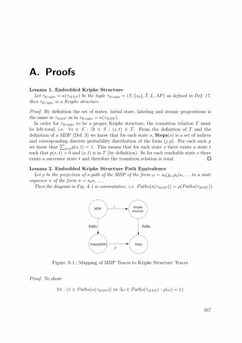
A. Proofs
Lemma 1. Embedded Kripke StructureLet τKripke = κ(τMDP ) be the tuple τKripke = (S, {s0}, T, L, AP ) as defined in Def. 17,
then τKripke is a Kripke structure.
Proof. By definition the set of states, initial state, labeling and atomic propositions isthe same in τMDP as in τKripke = κ(τMDP ).In order for τKripke to be a proper Kripke structure, the transition relation T must
be left-total, i.e. ∀s ∈ S : ∃t ∈ S : (s, t) ∈ T . From the definition of T and thedefinition of a MDP (Def. 3) we know that for each state s, Steps(s) is a set of indicesand corresponding discrete probability distribution of the form (j, p). For each such p
we know that∑
t∈S p(s, t) = 1. This means that for each state s there exists a state tsuch that p(s, t) > 0 and (s, t) is in T (by definition). So for each reachable state s thereexists a successor state t and therefore the transition relation is total.
Lemma 2. Embedded Kripke Structure Path EquivalenceLet ρ be the projection of a path of the MDP of the form ω = s0(j0, p0)s1 . . . to a state
sequence π of the form π = s0s1 . . ..Then the diagram in Fig. A.1 is commutative, i.e. Paths(κ(τMDP )) = ρ(Paths(τMDP )).
MDP
Paths(MDP)
Paths Paths
Kripkestructure
Paths
κ
ρ
Figure A.1.: Mapping of MDP Traces to Kripke Structure Traces
Proof. To show:
∀π : (π ∈ Paths(κ(τMDP )) ⇔ ∃ω ∈ Paths(τMDP ) : ρ(ω) = π)
167
A. Proofs
“⇒”:Let π be an arbitrary element of Paths(κ(τMDP )). As κ maps a MDP τMDP to
a Kripke structure τKripke with the same states, for each pair of states (s, t) in thetransition relation T of τKripke there exists an index, probability distribution pair (j, p)in τMDP such that p(s, t) > 0 holds (see Lemma (1)). Therefore for π = s0, s1 . . ., forevery pair (si, si+1) ∈ T there exists a pair (j, p) such that p(si, si+1) > 0 in the MDP andω = s0(j0, p0(s0, s1))s1 . . . is a path of τMDP (Def. (4)) and by its definition, ρ projectsω onto π (as the sequence of states is preserved)“⇐”:By contradiction: Assume ∃ω ∈ Paths(τMDP ) : ρ(ω) = π ∧ π 6∈ Paths(κ(τMDP )).
This means that for ω = s0(j0, p0)s1 . . . si(ji, pi)si+1 . . . the probability pi(si, si+1) = 0must hold (else π would be an element of Paths(κ(τMDP )), see Lemma (1)). But if sucha pair (ji, pi) exists, then ω is not a path of a MDP (see Def. (4)), as the probability toreach the next state must always be non-zero.
Corollary 1. Embedded Kripke Structure Trace EquivalenceA MDP τMDP and its embedded Kripke structure τKripke = κ(τMDP ) are isomorphic
wrt. their set of traces.
Proof. From Lemma 2, for each Path π = s′0s′1 . . . of the embedded Kripke structure
κ(τMDP ) there exists a Path ω = s0(j0, p0)s1 . . . of the MDP τMDP such that the projec-tion of ω is equal to π. The same holds vice versa.From the construction of the embedded Kripke structure (see Def. 17) the labeling
function for each state L(s0) is equal to L(s′0), as the labeling function is the same.
Lemma 3. Conservative IntegrationLet M be a SAML model with the set of state variables V ar and M ′ be the SAML
model in which the effect of a failure mode γi is integrated into M adhering to the rulesfor conservative integration. Let Fi be the corresponding failure module, failsi the statevariable that indicates that the failure mode is absent (failsi ≤ 0) or present (failsi >0). Let τMDP be the MDP corresponding to M and τ ′MDP be the MDP corresponding toM ′||Fi. Then:
∀π ∈ Paths(κ(τMDP )) : ∃π′ ∈ Paths(κ(τ ′MDP )) : π ≡ π′|V ar (A.1)
where π′|V ar is the projection of π′ onto the state variables v ∈ V ar
Proof. From the construction rules for failure effect modeling, it is assured that for alltraces for all states in which the failure mode is absent (the failure module is not instate “yes”), there exists a successor state with non-zero probability on which the failuremode is also absent1.
1This means that the occurrence pattern is modeled in a sensible way, so that the failure mode maynot appear at all and therefore the occurrence of the failure mode is not forced.
168

Therefore assume that
κ(τ ′MDP ), s0 |= AG (failsi ≤ 0 → EX(failsi ≤ 0)) (A.2)
holds. This means that for all states on all traces if the failure mode is absent, thenthere is also a successor state in which the failure mode is absent.
Then for each π ∈ Paths(κ(τMDP )) a corresponding π′ ∈ Paths(κ(τ ′MDP )) can beconstructed in the following way:
Let sk be the k− th state of a path π = s0, s1 . . . of κ(τMDP ). In the complete SAMLmodel, the activation condition that held in sk is of the form
∧mj=1 φj (the conjunction
of all active activation conditions of all parallel SAML modules).
Now let φt be the activation condition of the SAML module that was changed in M ′
to integrate the failure effect. Assume there exists a path π′ of κ(τ ′MDP ) on which forthe k − th state s′k failsi ≤ 0 holds and sk ≡ s′k|V ar, i.e. φt also holds in s′k.
Let sk+1 be a successor state of sk on π. As failsi ≤ 0 holds in s′k, any possiblesuccessor state s′k+1 on π′ cannot be a state introduced by the failure mode effectsmodeling (rule 3b). As φt ∧ failsi ≤ 0 holds in s′k there also exists a successor states′k+1 such that failsi ≤ 0 (because of (A.2)) and for which sk+1 ≡ s′k+1|V ar holds. Thereason is that all active update rules of the complete model of the original model Mhave a corresponding active update rule in M ′ if failsi ≤ 0 holds (and by constructionone which is active if failsi > 0 holds).
So for each path π of κ(τMDP ) for each state sk, if there exists an equivalent state s′k ona path π′ of κ(τ ′MDP ) on which failsi ≤ 0 holds, there exists an equivalent continuationof π and π′ such that π ≡ π′|V ar.
As the initial state does not change (rule 4), s0 ≡ s′0|V ar and failsi ≤ 0 ∈ L(s′0) holds(the absence of the failure mode is the initial state of the failure module in the describedfailure mode modeling) and the assertion follows by induction.
Lemma 4. Deductive Before Ordering / Strict Before Ordering
For an extended system model M+, a set of failure modes ∆, a predicate logic hazardH,a minimal critical set Γ and two failure modes γ1, γ2 ∈ Γ,
γ1 �Γ γ2 ⇔
κ(M+), π |= (ΓUH) → [(¬H ∧ ¬γ1 ∧ ¬γ2)
U(γ1 ∧ ((¬H ∧ ¬γ2)
U((γ2 ∧ ¬H) ∧ FH)))] (A.3)
169
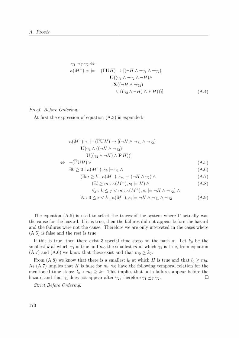
A. Proofs
γ1 ≺Γ γ2 ⇔
κ(M+), π |= (ΓUH) → [(¬H ∧ ¬γ1 ∧ ¬γ2)
U((γ1 ∧ ¬γ2 ∧ ¬H)∧
X((¬H ∧ ¬γ2)
U((γ2 ∧ ¬H) ∧ FH)))] (A.4)
Proof. Before Ordering:
At first the expression of equation (A.3) is expanded:
κ(M+), π |= (ΓUH) → [(¬H ∧ ¬γ1 ∧ ¬γ2)
U(γ1 ∧ ((¬H ∧ ¬γ2)
U((γ2 ∧ ¬H) ∧ FH))]
⇔ ¬(ΓUH) ∨ (A.5)
∃k ≥ 0 : κ(M+), sk |= γ1 ∧ (A.6)
(∃m ≥ k : κ(M+), sm |= (¬H ∧ γ2) ∧ (A.7)
(∃l ≥ m : κ(M+), sl |= H) ∧ (A.8)
∀j : k ≤ j < m : κ(M+), sj |= ¬H ∧ ¬γ2) ∧
∀i : 0 ≤ i < k : κ(M+), si |= ¬H ∧ ¬γ1 ∧ ¬γ2 (A.9)
The equation (A.5) is used to select the traces of the system where Γ actually wasthe cause for the hazard. If it is true, then the failures did not appear before the hazardand the failures were not the cause. Therefore we are only interested in the cases where(A.5) is false and the rest is true.
If this is true, then there exist 3 special time steps on the path π. Let k0 be thesmallest k at which γ1 is true and m0 the smallest m at which γ2 is true, from equation(A.7) and (A.6) we know that these exist and that m0 ≥ k0.
From (A.8) we know that there is a smallest l0 at which H is true and that l0 ≥ m0.As (A.7) implies that H is false for m0 we have the following temporal relation for thementioned time steps: l0 > m0 ≥ k0. This implies that both failures appear before thehazard and that γ1 does not appear after γ2, therefore γ1 �Γ γ2.
Strict Before Ordering:
170

κ(M+), π |= (ΓUH) → [(¬H ∧ ¬γ1 ∧ ¬γ2)
U((γ1 ∧ ¬γ2 ∧ ¬H) ∧
X((¬H ∧ ¬γ2)
U((γ2 ∧ ¬H) ∧ FH)))]
⇔ ¬(ΓUH) ∨ (A.10)
∃k ≥ 0 : (κ(M+), sk |= γ1 ∧ ¬γ2 ∧ ¬H) ∧
(∃m ≥ k + 1 : κ(M+), sm |= (γ2 ∧ ¬H)) ∧ (A.11)
(∃l ≥ m : κ(M+), sm |= H) ∧ (A.12)
(∀j : k ≤ j < m : κ(M+), sj |= ¬γ2 ∧ ¬H) ∧
(∀i : 0 ≤ i < k : κ(M+), si |= ¬γ1 ∧ ¬γ2 ∧ ¬H) (A.13)
Assume (A.10) to be false and the rest to be true for the reason mentioned before.Let k0 be the smallest k where γ1 ∧¬γ2 ∧¬H is true, let m0 be the smallest m where
γ2 ∧ ¬H is true and l0 the smallest l where H is true. From (A.11) we know thatm0 ≥ k0+1, i.e. m0 > k0 and from (A.12) and (A.11) we know that l0 > m0. Thereforewe know that if H appears on a trace, both failures appear before the hazard and γ1appears before γ2, i.e. γ1 ≺Γ γ2.
Lemma 5. Deductive Simultaneous OrderFor an extended system model M+, a set of failure modes ∆, a predicate logic hazard
H,a minimal critical set Γ and two failure modes γ1, γ2 ∈ Γ
γ1 ∼Γ γ2 ⇔
κ(M+), π |= (ΓUH) → [(¬H ∧ ¬γ1 ∧ ¬γ2)
U((γ1 ∧ γ2 ∧ ¬H) ∧ FH)] (A.14)
Proof. At first the expression of equation (A.14) is expanded:
κ(M+), π |= (ΓUH) → [(¬H ∧ ¬γ1 ∧ ¬γ2)
U((γ1 ∧ γ2 ∧ ¬H) ∧ FH))]
⇔ ¬(ΓUH) ∨ (A.15)
∃k ≥ 0 : κ(M+), sk |= (γ1 ∧ γ2 ∧ ¬H) (A.16)
∧(∃m ≥ k : κ(M+), sm |= H) ∧ (A.17)
∀i : 0 ≤ i < k : κ(M+), si |= ¬γ1 ∧ ¬γ2 ∧ ¬H (A.18)
Again, only the traces where Γ is the actual cause of H are of interest. Therefore weassume (A.15) to be false and the second part of the whole equation to be true.
171

A. Proofs
Let k0 be the smallest k where γ1 ∧ γ2 ∧ ¬H is true and m0 the smallest m where His true, then we know that m0 > k0 because H is false at k0 (A.16). On all time stepsbefore k0 both γ1 and γ2 are false (A.18). Therefore H appears after the failures andthe first time the failures appear, they appear together, i.e. γ1 ∼Γ γ2.
Lemma 6. aDCCA Completeness LemmaFor a complete aDCCA for an extended system model M+, a set of failure modes ∆
and a hazard H the following formula holds:
κ(M+), s0 |= A ((∧
Γ∈aMCSS(M+,∆,H)
¬∧
γj∈Γ
F γj) → ¬FGH)
Proof. By contradiction:
Assume:
κ(M+), s0 6|= A ((∧
Γ∈aMCSS(M+,∆,H)¬∧
γ∈Γ F γ) (A.19)
→ ¬FGH)
⇔ there exists π = s0, s1, . . . ∈ Paths(κ(M+)) : (A.20)
κ(M+), π |= (∧
Γ∈aMCSS(M+,∆,H) ¬∧
γ∈Γ F γ) (A.21)
and κ(M+), π |= FGH (A.22)
Since the set ∆ is finite, there is a state si on π such that all component failures γ ∈ ∆that will ever happen have occurred at least once. This means all failure modes thathave not appeared on π before si will not appear at all.
∀γ ∈ ∆ : (∀j < i : κ(M+), sj |= ¬γ) (A.23)
→ κ(M+), si |= G¬γ
Let Γ := {γ ∈ ∆ | ∃ j < i : κ(M+), sj |= γ} (A.24)
(A.22),(A.24)⇒ κ(M+), π |= (ΓU EG (H ∧ Γ))
⇔ Γ is adaptive-critical set (Def. 32)
⇒ ∃ Γ0 ⊆ Γ : Γ0 is minimal adaptive-critical set
therefore Γ0 ∈ aMCSS(M+,∆, H)
(A.24)⇒ κ(M+), π |=
∧
γ∈Γ F γ (A.25)
⇒ κ(M+), π |=∧
γ∈Γ0F γ, as Γ0 ⊆ Γ
⇒ κ(M+), π 6|= (∧
Γ∈aMCSS(M+,∆,H) ¬∧
γ∈Γ F γ)
⇒ contradiction to (A.20)
172
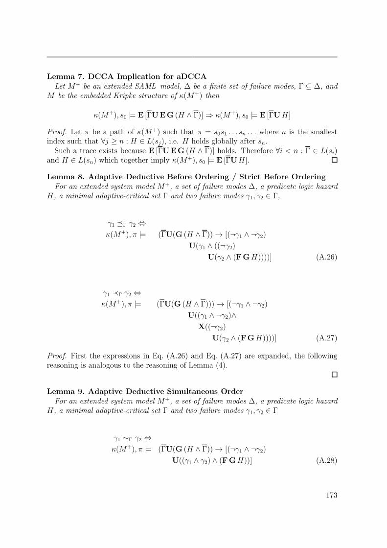
Lemma 7. DCCA Implication for aDCCALet M+ be an extended SAML model, ∆ be a finite set of failure modes, Γ ⊆ ∆, and
M be the embedded Kripke structure of κ(M+) then
κ(M+), s0 |= E [ΓUEG (H ∧ Γ)] ⇒ κ(M+), s0 |= E [ΓUH ]
Proof. Let π be a path of κ(M+) such that π = s0s1 . . . sn . . . where n is the smallestindex such that ∀j ≥ n : H ∈ L(sj), i.e. H holds globally after sn.Such a trace exists because E [ΓUEG (H ∧ Γ)] holds. Therefore ∀i < n : Γ ∈ L(si)
and H ∈ L(sn) which together imply κ(M+), s0 |= E [ΓUH ].
Lemma 8. Adaptive Deductive Before Ordering / Strict Before OrderingFor an extended system model M+, a set of failure modes ∆, a predicate logic hazard
H, a minimal adaptive-critical set Γ and two failure modes γ1, γ2 ∈ Γ,
γ1 �Γ γ2 ⇔
κ(M+), π |= (ΓU(G (H ∧ Γ)) → [(¬γ1 ∧ ¬γ2)
U(γ1 ∧ ((¬γ2)
U(γ2 ∧ (FGH))))] (A.26)
γ1 ≺Γ γ2 ⇔
κ(M+), π |= (ΓU(G (H ∧ Γ))) → [(¬γ1 ∧ ¬γ2)
U((γ1 ∧ ¬γ2)∧
X((¬γ2)
U(γ2 ∧ (FGH))))] (A.27)
Proof. First the expressions in Eq. (A.26) and Eq. (A.27) are expanded, the followingreasoning is analogous to the reasoning of Lemma (4).
Lemma 9. Adaptive Deductive Simultaneous OrderFor an extended system model M+, a set of failure modes ∆, a predicate logic hazard
H, a minimal adaptive-critical set Γ and two failure modes γ1, γ2 ∈ Γ
γ1 ∼Γ γ2 ⇔
κ(M+), π |= (ΓU(G (H ∧ Γ)) → [(¬γ1 ∧ ¬γ2)
U((γ1 ∧ γ2) ∧ (FGH))] (A.28)
173
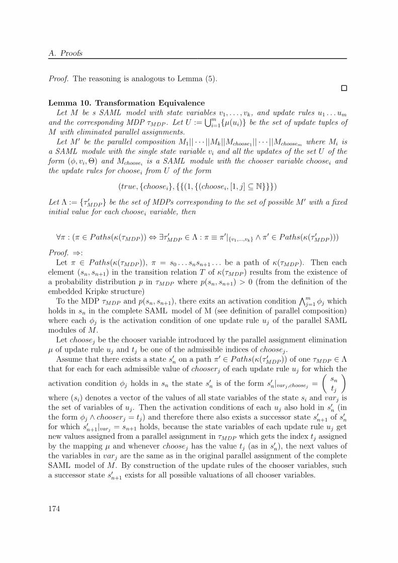
A. Proofs
Proof. The reasoning is analogous to Lemma (5).
Lemma 10. Transformation EquivalenceLet M be s SAML model with state variables v1, . . . , vk, and update rules u1 . . . um
and the corresponding MDP τMDP . Let U :=⋃m
i=1{µ(ui)} be the set of update tuples ofM with eliminated parallel assignments.Let M ′ be the parallel composition M1|| · · · ||Mk||Mchoose1|| · · · ||Mchoosem where Mi is
a SAML module with the single state variable vi and all the updates of the set U of theform (φ, vi,Θ) and Mchoosei is a SAML module with the chooser variable choosei andthe update rules for choosei from U of the form
(true, {choosei}, {{(1, {(choosei, [1, j] ⊆ N}}})
Let Λ := {τ ′MDP} be the set of MDPs corresponding to the set of possible M ′ with a fixedinitial value for each choosei variable, then
∀π : (π ∈ Paths(κ(τMDP )) ⇔ ∃τ ′MDP ∈ Λ : π ≡ π′|{v1,...,vk} ∧ π′ ∈ Paths(κ(τ ′MDP )))
Proof. ⇒:Let π ∈ Paths(κ(τMDP )), π = s0 . . . snsn+1 . . . be a path of κ(τMDP ). Then each
element (sn, sn+1) in the transition relation T of κ(τMDP ) results from the existence ofa probability distribution p in τMDP where p(sn, sn+1) > 0 (from the definition of theembedded Kripke structure)To the MDP τMDP and p(sn, sn+1), there exits an activation condition
∧mj=1 φj which
holds in sn in the complete SAML model of M (see definition of parallel composition)where each φj is the activation condition of one update rule uj of the parallel SAMLmodules of M .Let choosej be the chooser variable introduced by the parallel assignment elimination
µ of update rule uj and tj be one of the admissible indices of choosej .Assume that there exists a state s′n on a path π′ ∈ Paths(κ(τ ′MDP )) of one τMDP ∈ Λ
that for each for each admissible value of chooserj of each update rule uj for which the
activation condition φj holds in sn the state s′n is of the form s′n|varj ,choosej =
(
sntj
)
where (si) denotes a vector of the values of all state variables of the state si and varj isthe set of variables of uj. Then the activation conditions of each uj also hold in s′n (inthe form φj ∧ chooserj = tj) and therefore there also exists a successor state s′n+1 of s′nfor which s′n+1|varj = sn+1 holds, because the state variables of each update rule uj getnew values assigned from a parallel assignment in τMDP which gets the index tj assignedby the mapping µ and whenever choosej has the value tj (as in s′n), the next values ofthe variables in varj are the same as in the original parallel assignment of the completeSAML model of M . By construction of the update rules of the chooser variables, sucha successor state s′n+1 exists for all possible valuations of all chooser variables.
174
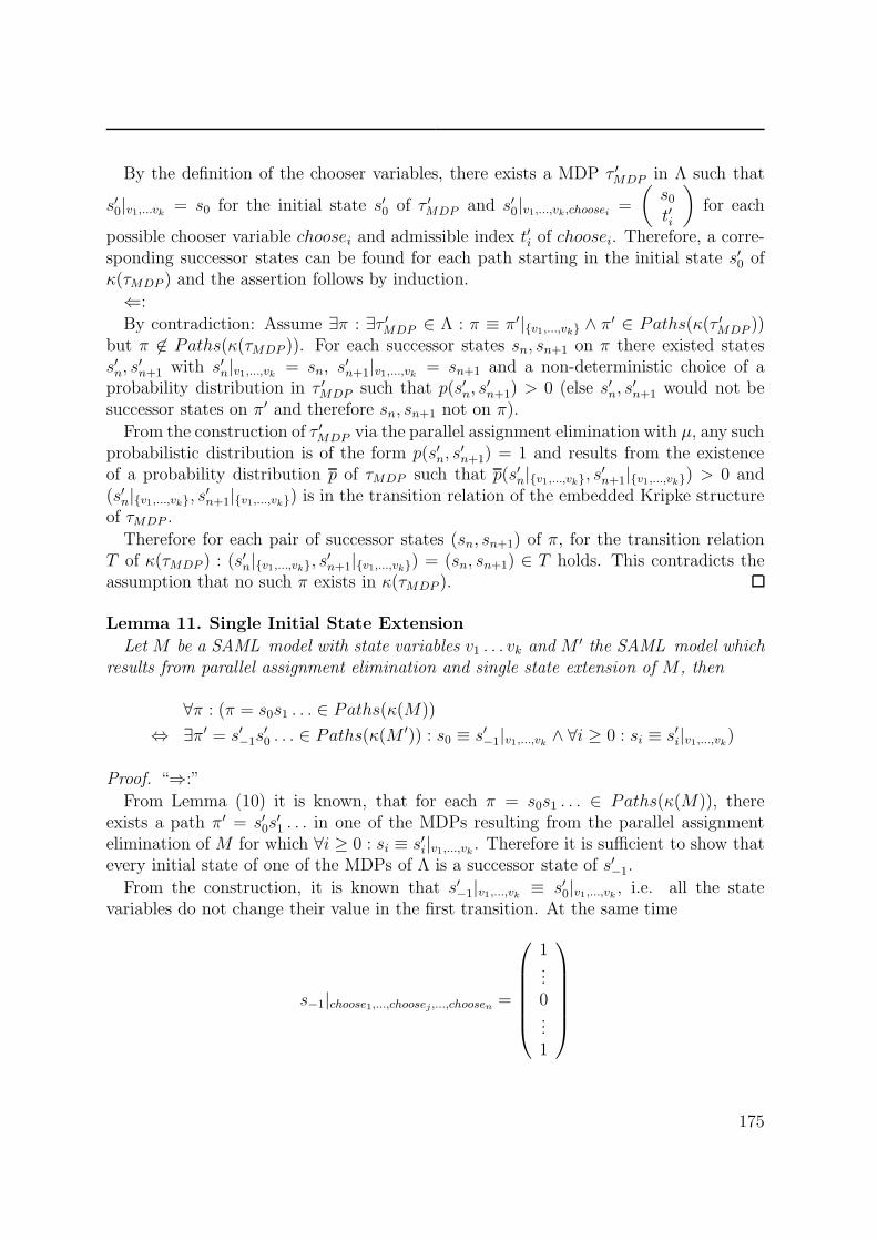
By the definition of the chooser variables, there exists a MDP τ ′MDP in Λ such that
s′0|v1,...vk = s0 for the initial state s′0 of τ ′MDP and s′0|v1,...,vk,choosei =
(
s0t′i
)
for each
possible chooser variable choosei and admissible index t′i of choosei. Therefore, a corre-sponding successor states can be found for each path starting in the initial state s′0 ofκ(τMDP ) and the assertion follows by induction.
⇐:
By contradiction: Assume ∃π : ∃τ ′MDP ∈ Λ : π ≡ π′|{v1,...,vk} ∧ π′ ∈ Paths(κ(τ ′MDP ))
but π 6∈ Paths(κ(τMDP )). For each successor states sn, sn+1 on π there existed statess′n, s
′n+1 with s′n|v1,...,vk = sn, s
′n+1|v1,...,vk = sn+1 and a non-deterministic choice of a
probability distribution in τ ′MDP such that p(s′n, s′n+1) > 0 (else s′n, s
′n+1 would not be
successor states on π′ and therefore sn, sn+1 not on π).
From the construction of τ ′MDP via the parallel assignment elimination with µ, any suchprobabilistic distribution is of the form p(s′n, s
′n+1) = 1 and results from the existence
of a probability distribution p of τMDP such that p(s′n|{v1,...,vk}, s′n+1|{v1,...,vk}) > 0 and
(s′n|{v1,...,vk}, s′n+1|{v1,...,vk}) is in the transition relation of the embedded Kripke structure
of τMDP .
Therefore for each pair of successor states (sn, sn+1) of π, for the transition relationT of κ(τMDP ) : (s
′n|{v1,...,vk}, s
′n+1|{v1,...,vk}) = (sn, sn+1) ∈ T holds. This contradicts the
assumption that no such π exists in κ(τMDP ).
Lemma 11. Single Initial State Extension
Let M be a SAML model with state variables v1 . . . vk and M ′ the SAML model whichresults from parallel assignment elimination and single state extension of M , then
∀π : (π = s0s1 . . . ∈ Paths(κ(M))
⇔ ∃π′ = s′−1s′0 . . . ∈ Paths(κ(M ′)) : s0 ≡ s′−1|v1,...,vk ∧ ∀i ≥ 0 : si ≡ s′i|v1,...,vk)
Proof. “⇒:”
From Lemma (10) it is known, that for each π = s0s1 . . . ∈ Paths(κ(M)), thereexists a path π′ = s′0s
′1 . . . in one of the MDPs resulting from the parallel assignment
elimination of M for which ∀i ≥ 0 : si ≡ s′i|v1,...,vk . Therefore it is sufficient to show thatevery initial state of one of the MDPs of Λ is a successor state of s′−1.
From the construction, it is known that s′−1|v1,...,vk ≡ s′0|v1,...,vk , i.e. all the statevariables do not change their value in the first transition. At the same time
s−1|choose1,...,choosej,...,choosen =
1...0...1
175
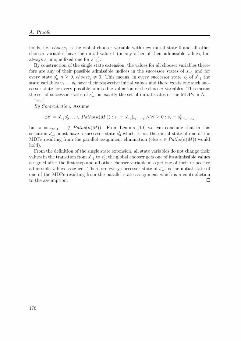
A. Proofs
holds, i.e. choosej is the global chooser variable with new initial state 0 and all otherchooser variables have the initial value 1 (or any other of their admissible values, butalways a unique fixed one for s−1).By construction of the single state extension, the values for all chooser variables there-
fore are any of their possible admissible indices in the successor states of s−1 and forevery state s′n, n ≥ 0, choosej 6= 0. This means, in every successor state s′0 of s′−1 thestate variables v1 . . . vk have their respective initial values and there exists one such suc-cessor state for every possible admissible valuation of the chooser variables. This meansthe set of successor states of s′−1 is exactly the set of initial states of the MDPs in Λ.“⇐:”By Contradiction: Assume
∃π′ = s′−1s′0 . . . ∈ Paths(κ(M ′)) : s0 ≡ s′−1|v1,...,vk ∧ ∀i ≥ 0 : si ≡ s′i|v1,...,vk
but π = s0s1 . . . 6∈ Paths(κ(M)). From Lemma (10) we can conclude that in thissituation s′−1 must have a successor state s′0 which is not the initial state of one of theMDPs resulting from the parallel assignment elimination (else π ∈ Paths(κ(M)) wouldhold).From the definition of the single state extension, all state variables do not change their
values in the transition from s′−1 to s′0, the global chooser gets one of its admissible values
assigned after the first step and all other chooser variable also get one of their respectiveadmissible values assigned. Therefore every successor state of s′−1 is the initial state ofone of the MDPs resulting from the parallel state assignment which is a contradictionto the assumption.
176

B. Peer-Reviewed Publications
• 2011
– Model-Based Multi-Objective Safety Optimization Matthias Gudemann, FrankOrtmeier, Proceedings of the 30th International Conference on ComputerSafety, Reliability and Security (SAFECOMP 2011), Springer LNCS (to ap-pear 19.9.2011)
– Towards Model-driven Safety Analysis Matthias Gudemann, Frank Ortmeier,Proceedings of the 3rd International Workshop On Dependable Control OfDiscrete Systems (DCDS 2011), IEEE
• 2010
– A Framework for Qualitative and Quantitative Model-Based Safety AnalysisMatthias Gudemann, Frank Ortmeier, Proceedings of the 12th High AssuranceSystem Engineering Symposium (HASE 2010)
– Quantitative Model-Based Safety Analyis: A Case Study Matthias Gudemann,Frank Ortmeier, Proceedings of the 5th conference for Sicherheit, Schutz undZuverlaessigkeit (SICHERHEIT 2010), Lecture Notes in Informatics (LNI)
– SysML in Digital Engineering Matthias Gudemann, Stefan Kegel, Frank Ort-meier, Olaf Poenicke, Klaus Richter, Proceedings of the 1st InternationalWorkshop on Digital Engineering (IWDE 2010), ACM Digital Library
– Probabilistic Model-Based Safety Analysis Matthias Gudemann, Frank Ort-meier, Proceedings of the 8th Workshop of Quantitative Aspects of Program-ming Languages (QAPL 2010) at ETAPS 2010, EPTCS
– ProMoSA - Probabilistic Models for Safety Analysis Frank Ortmeier, MatthiasGudemann Modellbasierte Entwicklung eingebetteter Systeme (MBEES 2010),03.02.2010 - 05.02.2010, Schloss Dagstuhl
• 2008
– Computing Ordered Minimal Critical Sets Matthias Gudemann, Frank Ort-meier, Wolfgang Reif Proceedings of Formal Methods for Automation andSafety in Railway and Automotive Systems (FORMS / FORMAT 2008) (eds.G. Tarnai & E. Schnieder)
177
B. Peer-Reviewed Publications
– A specification and construction paradigm for Organic Computing systemsM. Gudemann, F.Nafz, F.Ortmeier, H.Seebach and W.Reif, Proceedings ofthe 2nd IEEE International Conference on Self-Adaptive and Self-OrganizingSystems (SASO 2008), IEEE Computer Society Press
– Developing Safety-Critical Mechatronical Systems Matthias Gudemann, FrankOrtmeier, Wolfgang Reif 7. Internationales Heinz Nixdorf Symposium: Selb-stoptimierende mechatronische Systeme, HNI Schriftenreihe
• 2007
– Using Deductive Cause-Consequenc Analysis (DCCA) with SCADE MatthiasGudemann, Frank Ortmeier, Wolfgang Reif Proceedings of 27th SAFECOMP2007, LNCS 4680, Springer, LNCS
– Formal Failure Models Frank Ortmeier, Matthias Gudemann, Wolfgang ReifProceedings of the 1st IFAC Workshop on Dependable Control of DiscreteSystems (DCDS 2007), Elsevier
– Modeling of self-adaptive systems with SCADE Matthias Gudemann, An-dreas Angerer, Frank Ortmeier, Wolfgang Reif Proceedings of the 40th IEEEInternational Symposium on Circuits and Systems (ISCAS 2007), IEEE
• 2006
– Safety and Dependability Analysis of Self-Adaptive Systems M. Gudemann, F.Ortmeier, W. Reif Proceedings of the 2nd International Symposium on Lever-aging Applications of Formal Methods, Verification and Validation (ISoLA2006), IEEE Computer Society Press
– Towards Safe and Secure Organic Computing Applications Matthias Gude-mann, Florian Nafz, Wolfgang Reif and Hella Seebach C. Hochberger and R.Liskowsky, editors, INFORMATIK 2006 – Informatik fur Menschen, volumeP-93 of GI-Edition – Lecture Notes in Informatics, Kollen Verlag
– Formal Modeling and Verification of Systems with Self-x Properties MatthiasGudemann, Frank Ortmeier and Wolfgang Reif Proceedings of the 3rd In-ternational Conference on Autonomic and Trusted Computing (ATC 2006),Springer
178
Bibliography
[ADS+04] Parosh Aziz Abdulla, Johann Deneux, Gunnar Stalmarck, Herman Agren,and Ove Akerlund. Designing safe, reliable systems using SCADE. In Pro-ceedings of the 1st International Symposium on Leveraging Applications ofFormal Methods, Verification and Validation (ISoLA 04). Springer, 2004.
[AFG+09] Husain Aljazzar, Manuel Fischer, Lars Grunske, Matthias Kuntz, FlorianLeitner-Fischer, and Stefan Leue. Safety analysis of an airbag system usingprobabilistic fmea and probabilistic counterexamples. In Proceedings ofthe 2009 Sixth International Conference on the Quantitative Evaluation ofSystems (QEST 2009), pages 299–308, Washington, DC, USA, 2009. IEEEComputer Society.
[AK09] Robert Alexander and Tim Kelly. Escaping the non-quantitative trap.In Proceedings of the 27th International System Safety Conference (ISSC2009), 2009.
[AKLFL10] Husain Aljazzar, Matthias Kuntz, Florian Leitner-Fischer, and StefanLeue. Directed and heuristic counterexample generation for probabilis-tic model checking: a comparative evaluation. In Proceedings of the 2010ICSE Workshop on Quantitative Stochastic Models in the Verification andDesign of Software Systems (QUOVADIS 2010), pages 25–32, New York,NY, USA, 2010. ACM.
[APGR99] Andre Arnold, Gerald Point, Alain Griffault, and Antoine Rauzy. Thealtarica formalism for describing concurrent systems. Fundam. Inf., 40:109–124, November 1999.
[AVA03] AVACS. Automatic verification and analysis of complex systems. Technicalreport, University of Oldenburg, 2003.
[B+03] M. Bozzano et al. ESACS: An integrated methodology for design andsafety analysis of complex systems. In Proceedings of European Safetyand Reliability Conference (ESREL 2003), pages 237–245, Maastricht, TheNetherlands, 2003. Balkema publisher.
[BaFV04] B. Berthomieu and P.-O. Ribet an F. Vernadat. The tool tina - constructionof abstract state spaces for petri nets and time petri nets. InternationalJournal of Production Research, 42, 2004.
179

Bibliography
[BB03] Marc Bouissou and Jean-Louis Bon. A new formalism that combines ad-vantages of fault-trees and markov models: Boolean logic driven markovprocesses. Reliability Engineering & System Safety, 82(2):149 – 163, 2003.
[BBC+04] Pierre Bieber, Christian Bougnol, Charles Castel, Jean pierre Heckmann,Christophe Kehren, Sylvain Metge, Christel Seguin, P. Bieber, C. Bougnol,C. Castel, J. p. Heckmann, C. Kehren, and C. Seguin. Safety assessmentwith altarica - lessons learnt based on two aircraft system studies. InProceedings of the 18th IFIP World Computer Congress, Topical Day onNew Methods for Avionics Certification, page 26, 2004.
[BBC+08] Jiri Barnat, Lubos Brim, Ivana Cerna, Milan Ceska, and Jana Tumova.ProbDiVinE-MC: Multi-core LTL Model Checker for Probabilistic Sys-tems. In Proceedings of the 5th International Conference on QuantitativeEvaluation of Systems (QEST 2008), pages 77–78, 2008.
[BBR08] M. Balser, S. Baumler, and W. Reif. An interval temporal logic with com-positional interleaving. Technical Report 2008-20, University of Augsburg,2008.
[BCF+08] Roberto Bruttomesso, Alessandro Cimatti, Anders Franzen, Alberto Grig-gio, and Roberto Sebastiani. The mathsat 4 smt solver. In Aarti Guptaand Sharad Malik, editors, Proceedings of the International Conference onComputer Aided Verification (CAV 2008), volume 5123 of Lecture Notesin Computer Science, pages 299–303. Springer Berlin / Heidelberg, 2008.
[BCK+09a] Marco Bozzano, Alessandro Cimatti, Joost-Pieter Katoen, Viet YenNguyen, Thomas Noll, and Marco Roveri. COMPASS project webpage.http://compass.informatik.rwth-aachen.de/, 2009.
[BCK+09b] Marco Bozzano, Alessandro Cimatti, Joost-Pieter Katoen, Viet YenNguyen, Thomas Noll, and Marco Roveri. Model-based codesign of criticalembedded systems. In Proceedings of the 2nd International Workshop onModel Based Architecting and Construction of Embedded Systems (ACES-MB 2009), volume 507, pages 87–91. CEUR Workshop Proceedings, 2009.
[BCK+10a] Marco Bozzano, Alessandro Cimatti, Joost-Pieter Katoen, Viet Nguyen,Thomas Noll, Marco Roveri, and Ralf Wimmer. A model checker forAADL. In Tayssir Touili, Byron Cook, and Paul Jackson, editors, Proceed-ings of the Computer Aided Verification Conference (CAV 2010), volume6174 of Lecture Notes in Computer Science, pages 562–565. Springer Berlin/ Heidelberg, 2010.
180

Bibliography
[BCK+10b] Marco Bozzano, Alessandro Cimatti, Joost-Pieter Katoen, Viet YenNguyen, Thomas Noll, and Marco Roveri. Safety, dependability, and per-formance analysis of extended AADL models. The Computer Journal,2010.
[BCM+90] J. R. Burch, E. M. Clarke, K. L. McMillan, D. L. Dill, and L. J. Hwang.Symbolic model checking: 1020 states and beyond. In Proceedingsof the5th Annual IEEE Symposium on Logic in Computer Science (LICS 1990),pages 428–439, Philadelphia, Pennsylvania, 1990. IEEE Computer SocietyPress.
[BCR+09] Marco Bozzano, Alessandro Cimatti, Marco Roveri, Joost-Pieter Katoen,Viet Yen Nguyen, and Thomas Noll. Verification and performance evalu-ation of AADL models. In Proceedings of the the 7th joint meeting of theEuropean software engineering conference and the ACM SIGSOFT sym-posium on The foundations of software engineering (ESEC/FSE 2009),ESEC/FSE ’09, pages 285–286, New York, NY, USA, 2009. ACM.
[BCS02] P. Bieber, C. Castel, and C. Seguin. Combination of fault tree analysis andmodel checking for safety assessment of complex systems. In Proceedings ofthe 4th European Dependable Computing Conference (EDCC 2002), volume2485 of LNCS, pages 19–31, Toulouse, France, 2002. Springer-Verlag.
[BCS07a] Hichem Boudali, Pepijn Crouzen, and Marielle Stoelinga. A compositionalsemantics for dynamic fault trees in terms of interactive markov chains. InProceedings of the 5th international conference on Automated technologyfor verification and analysis (ATVA 2007), pages 441–456, Berlin, Heidel-berg, 2007. Springer-Verlag.
[BCS07b] Hichem Boudali, Pepijn Crouzen, and Marielle Stoelinga. Dynamic faulttree analysis using input/output interactive markov chains. In Proceedingsof the 37th Annual IEEE/IFIP International Conference on DependableSystems and Networks (DSN 2007), pages 708–717, Washington, DC, USA,2007. IEEE Computer Society.
[BD04] Simona Bernardi and Susanna Donatelli. Stochastic petri nets and inheri-tance for dependability modelling. In Proceedings of the 10th IEEE PacificRim International Symposium on Dependable Computing (PRDC 2004),pages 363 – 372, march 2004.
[BDW00] T. Bienmoller, W. Damm, and H. Wittke. The STATEMATE verificationenvironment – making it real. In E. A. Emerson and A. P. Sistla, editors,Proceedings of the 12th international Conference on Computer Aided Ver-ification (CAV 2000), number 1855 in LNCS, pages 561–567, Chicago, IL,USA, 2000. Springer.
181

Bibliography
[BES09] D. Bosnacki, S. Edelkamp, and D. Sulewski. Efficient probabilistic modelchecking on general purpose graphics processors. In C. Pasareanu, editor,Proceedings of the 16th International SPIN Workshop (SPIN 2009), volume5578 of LNCS, pages 32–49. Springer, 2009.
[BF93] Ricky W. Butler and George B. Finelli. The infeasibility of quantifying thereliability of life-critical real-time software. IEEE Transactions on SoftwareEngineering, 19:3–12, 1993.
[Bit01] Friedemann Bitsch. Safety patterns - the key to formal specification ofsafety requirements. In Udo Voges, editor, Proceedings of the 20th nter-national Conference on Computer Safety, Reliability and Security (SAFE-COMP 2001), volume 2187 of LNCS, pages 176–189. Springer Berlin /Heidelberg, 2001.
[BK86] J.A. Bergstra and J.W. Klop. Algebra of communicating processes. InProceedings CWI Symposium Mathematical and Computer Science, CWIMonographs I series, 1986.
[Bou07] Marc Bouissou. A generalization of dynamic fault trees through booleanlogic driven markov processes (BDMP) R©. In Proceedings of the EuropeanSafety and Reliability Conference (ESREL 2007). Springer-Verlag, 2007.
[Boz11] Marco Bozzano. Automated Generation of Compact FMEA Tables in theCOMPASS Toolset. Talk at CISEC Model Based Safety Assessment Work-shop (MBSAW 2011), 2011. accessed April 2011.
[BPRW08a] Eckard Bode, Thomas Peikenkamp, Jan Rakow, and Samuel Wischmeyer.Model based importance analysis for minimal cut sets. Reports of SFB/TR14 AVACS 29, SFB/TR 14 AVACS, Apr 2008. ISSN: 1860-9821.
[BPRW08b] Eckard Bode, Thomas Peikenkamp, Jan Rakow, and Samuel Wischmeyer.Model based importance analysis for minimal cut sets. In Sung DeokCha, Jin-Young Choi, Moonzoo Kim, Insup Lee, and Mahesh Viswanathan,editors, Proceedings of the 6th International Symbposium on AutomatedTechnology for Verification and Analysis (ATVA 2008), volume 5311 ofLNCS, pages 303–317, 2008.
[BV03a] M. Bozzano and A. Villafiorita. Integrating fault tree analysis with eventordering information. In Proceedings of Proceedings of the European Safety& Reliability Conference (ESREL 2003), pages 247–254. Balkema, 2003.
[BV03b] M. Bozzano and Adolfo Villafiorita. Improving system reliability via modelchecking: the FSAP/NuSMV-SA safety analysis platform. In Proceedings
182
Bibliography
of the 22nd International Conference on Computer Safety, Reliability andSecurity (SAFECOMP 2003), pages 49–62. Springer, 2003.
[CAB+01] W. Chan, R. J. Anderson, P. Beame, D. H. Jones, D. Notkin, and W. E.Warner. Optimizing symoblic model checking for statecharts. IEEE Trans-actions on Software Engineering, 27(2):170 – 190, 2001.
[CBRZ01] Edmund Clarke, Armin Biere, Richard Raimi, and Yunshan Zhu. Boundedmodel checking using satisfiability solving. In Formal Methods in SystemDesign, page 2001, 2001.
[CCG+02] A. Cimatti, E. Clarke, E. Giunchiglia, F. Giunchiglia, M. Pistore,M. Roveri, R. Sebastiani, and A. Tacchella. NuSMV Version 2: An Open-Source Tool for Symbolic Model Checking. In Proceedings of the 14th Inter-national Conference on Computer Aided Verification (CAV 2002), volume2404 of LNCS. Springer, 2002.
[CCOR11] Roberto Cavada, Alessandro Cimatti, Emanuele Olivetti, and Marco Pi-storeand Marco Roveri. NuSMV v2.5 User Manual, accessed: January2011.
[CdAFL09] Krishnendu Chatterjee, Luca de Alfaro, Marco Faella, and Axel Legay.Qualitative logics and equivalences for probabilistic systems. Logical Meth-ods in Computer Science, 5(2), 2009.
[CG04] Frank Ciesinski and Marcus Großer. On probabilistic computation treelogic. In Christel Baier, Boudewijn R. Haverkort, Holger Hermanns, Joost-Pieter Katoen, and Markus Siegle, editors, Validation of Stochastic Sys-tems, volume 2925 of LNCS, pages 147–188. Springer, 2004.
[CGP00] E. Clarke, O. Grumberg, and D. Peled. Model Checking. MIT Press, 2000.
[CH00] E. M. Clarke and W. Heinle. Modular translation of statecharts to smv.Technical report, School of Computer Science, Carnegie Mellon University,2000.
[Cla08] Edmund Clarke. The birth of model checking. In Orna Grumberg andHelmut Veith, editors, 25 Years of Model Checking, volume 5000 of LNCS,pages 1–26. Springer, 2008.
[CMZ02] A. Cau, B. Moszkowski, and H. Zedan. ITL – Interval Tempo-ral Logic. Software Technology Research Laboratory, SERCentre, DeMontfort University, The Gateway, Leicester LE1 9BH, UK, 2002.www.cms.dmu.ac.uk/∼cau/itlhomepage.
183
Bibliography
[CR05] Daniele Codetta-Raiteri. The conversion of dynamic fault trees to stochas-tic petri nets, as a case of graph transformation. In Proceedings of theWorkshop on Petri Nets and Graph Transformations (PNGT 2004), pages45 – 60. ENTCS, 2005.
[dAFH+05] Luca de Alfaro, Marco Faella, Thomas A. Henzinger, Rupak Majumdar,and Marielle Stoelinga. Model checking discounted temporal properties.Theoretical Computer Science, 345:139–170, 2005.
[dAKN+00] L. de Alfaro, M. Kwiatkowska, G. Norman, D. Parker, and R. Segala.Symbolic model checking of probabilistic processes using MTBDDs andthe Kronecker representation. In S. Graf and M. Schwartzbach, editors,Proceedings of the 6th International Conference on Tools and Algorithmsfor the Construction and Analysis of Systems (TACAS 2000), volume 1785of LNCS, pages 395–410. Springer, 2000.
[Dow97] Mark Dowson. The ariane 5 software failure. SIGSOFT Softw. Eng. Notes,22:84–, March 1997.
[ea03] M. Bozzano et al. ESACS: An integrated methodology for design and safetyanalysis of complex systems. In Proceedings of the European Conferenceon Safety and Reliability (ESREL 2003), 2003.
[Est11] Esterel Technologies, http://www.esterel-technologies.com/?id=13281, ac-cessed Feb. 28. 2011. SCADE Suite, 2011.
[FGK+96] Jean-Claude Fernandez, Hubert Garavel, Alain Kerbrat, Laurent Mounier,Radu Mateescu, and Mihaela Sighireanu. CADP - a protocol validationand verification toolbox, 1996.
[FGP+08] Patrick Farail, Pierre Gaufillet, Florent Peres, Jean-Paul Bodeveix,Mamoun Filali, B. Berthomieu, Saad Rodrigo, F. Vernadat, Hubert Gar-avel, and Frederic Lang. FIACRE: an intermediate language for modelverification in the TOPCASED environment. In European Congress onEmbedded Real-Time Software (ERTS 2008), http://www.see.asso.fr, jan-vier 2008. SEE.
[FM92] Peter Fenelon and John A. McDermid. New directions in software safety:Causal modelling as an aid to integration. Technical report, High IntegritySystems Engineering Group, Department of Computer Science, Universityof York, 1992.
[FM93] Peter Fenelon and John A McDermid. An integrated tool set for soft-ware safety analysis. Journal of Systems and Software, 21(3):279 – 290,
184
Bibliography
1993. Applying Specification, Verification, and Validation Techniques toIndustrial Software Systems.
[GCW07] L. Grunske, R. Colvin, and K. Winter. Probabilistic model-checking sup-port for FMEA. In Proceedings of the 4th International Conference onQuantitative Evaluation of Systems (QEST 2007). IEEE, 2007.
[GH08] L. Grunske and Jun Han. A comparative study into architecture-basedsafety evaluation methodologies using aadl’s error annex and failure prop-agation models. In Proceedings of the 11th High Assurance Systems Engi-neering Symposium (HASE 2008), pages 283 –292, 2008.
[GLYW05] Lars Grunske, Peter Lindsay, Nisansala Yatapanage, and Kirsten Winter.An automated failure mode and effect analysis based on high-level designspecification with behavior trees. In Judi Romijn, Graeme Smith, and Jacovan de Pol, editors, Integrated Formal Methods, volume 3771 of LectureNotes in Computer Science, pages 129–149. Springer, 2005.
[GMMP02] A. Galloway, J.A. McDermid, J. Murdoch, and D.J. Pumfrey. Automationof system safety analysis: Possibilities and pitfalls. In Porceedings of the20th International System Safety Conference (ISSC 2002), 2002.
[GNO+08] M. Gudemann, F. Nafz, F. Ortmeier, H. Seebach, and W. Reif. A speci-fication and construction paradigm for Organic Computing systems. InSven Brueckner, Paul Robertson, and Umesh Bellur, editors, Proceed-ings of the 2nd IEEE International Conference on Self-Adaptive and Self-Organizing Systems (SASO 2008), pages 233–242. IEEE Computer SocietyPress (2008), 2008.
[GO10a] Matthias Gudemann and Frank Ortmeier. A framework for qualitative andquantitative model-based safety analysis. In Proceedings of the 12th HighAssurance System Engineering Symposium (HASE 2010), 2010.
[GO10b] Matthias Gudemann and Frank Ortmeier. Probabilistic model-based safetyanalysis. In Proceedings of the 8th Workshop on Quantitative Aspects ofProgramming Languages (QAPL 2010). EPTCS, 2010.
[GO10c] Matthias Gudemann and Frank Ortmeier. Quantitative model-based safetyanalysis: A case study. In Proceedings of 5th conference for Sicherheit,Schutz und Zuverlaessigkeit (SICHERHEIT 2010). Lecture Notes in Infor-matics (LNI), 2010.
[GO11a] Matthias Gudemann and Frank Ortmeier. Model-Based Multi-ObjectiveSafety Optimization. In Proceedings of the 30th International Conference
185
Bibliography
on Computer Safety, Reliability and Security (SAFECOMP 2011). SpringerLNCS, 2011. to appear: 19.9.2011.
[GO11b] Matthias Gudemann and Frank Ortmeier. Towards Model-driven SafetyAnalysis. In Proceedings of the 3rd international Workshop on DependableControl of Discrete Systems (DCDS 2011). IEEE, 2011.
[GOR06a] M. Gudemann, F. Ortmeier, and W. Reif. Formal modeling and verificationof systems with self-x properties. In Laurence T. Yang, Hai Jin, JianhuaMa, and Theo Ungerer, editors, Proceedings of the Third InternationalConference on Autonomic and Trusted Computing (ATC 2006), LNCS,pages 38–47. Springer, September 2006.
[GOR06b] M. Gudemann, F. Ortmeier, and W. Reif. Safety and dependability anal-ysis of self-adaptive systems. In Proceedings of the 2nd International Sym-posium on Leveraging Applications of Formal Methods, Verification andValidation (ISoLA 2006). IEEE CS Press, 2006.
[GOR07] Matthias Gudemann, Frank Ortmeier, and Wolfgang Reif. Using deductivecause consequence analysis (DCCA) with SCADE. In Proceedings of the26th International Conference on Computer Safety, Reliability and Security(SAFECOMP 2007). Springer LNCS 4680, 2007.
[GOR08] M. Gudemann, F. Ortmeier, and W. Reif. Computing ordered minimalcritical sets. In E. Schnieder and G. Tarnai, editors, Proceedings of the 7th
Symposium on Formal Methods for Automation and Safety in Railway andAutomotive Systems (FORMS/FORMAT 2008), 2008.
[GPM09] Xiaocheng Ge, Richard F. Paige, and John A. McDermid. Probabilistic fail-ure propagation and transformation analysis. In Bettina Buth, Gerd Rabe,and Till Seyfarth, editors, Proceedings of the 28th International Conferenceon Computer Safety, Reliability and Security (SAFECOMP 2009), LNCS,pages 215–228. Springer, 2009.
[Gro06] OMG Object Modeling Group. The unified modeling language, 2006.
[Gru08] Lars Grunske. Specification patterns for probabilistic quality properties. InProceedings of the 30th international conference on Software engineering(ICSE 2008), pages 31–40, New York, NY, USA, 2008. ACM.
[GV04] Alain Griffault and Aymeric Vincent. The Mec 5 model-checker. In Pro-ceedings of the International Conference on Computer Aided Verification(CAV 2004), volume 3114 of LNCS, pages 488–491. Springer, July 2004.
186

Bibliography
[HCRP91] N. Halbwachs, P. Caspi, P. Raymond, and D. Pilaud. The synchronousdata-flow programming language Lustre. Proceedings of the IEEE,79(9):1305–1320, September 1991.
[HJ94] Hans Hansson and Bengt Jonsson. A logic for reasoning about time andreliability. Formal Aspects of Computing, 6:102–111, 1994.
[HK98] Michael Huth and Martha Z. Kwiatkowska. Comparing ctl and pctl on la-beled markov chains. In Proceedings of the IFIP TC2/WG2.2,2.3 Interna-tional Conference on Programming Concepts and Methods (PROCOMET1998), pages 244–262, London, UK, UK, 1998. Chapman & Hall, Ltd.
[HKB09] Tingting Han, Joost-Pieter Katoen, and Damman Berteun. Counterexam-ple generation in probabilistic model checking. IEEE Trans. Softw. Eng.,35(2):241–257, 2009.
[HKMKS00] Holger Hermanns, Joost-Pieter Katoen, Joachim Meyer-Kayser, andMarkus Siegle. A markov chain model checker. In Proceedings of the 6th
International Conference on Tools and Algorithms for Construction andAnalysis of Systems (TACAS 2000), pages 347–362. Springer, 2000.
[HN96] D. Harel and A. Naamad. The statemate semantics of statecharts. ACMTransactions on Software Engineering and Methodology, 5(4):293–333, Oc-tober 1996.
[HWP+06] Marc Herbstritt, Ralf Wimmer, Thomas Peikenkamp, Eckard Bode,Michael Adelaide, Sven Johr, Holger Hermanns, and Bernd Becker. Anal-ysis of Large Safety-Critical Systems: A quantitative Approach. Reportsof SFB/TR 14 AVACS 8, SFB/TR 14 AVACS, Feb 2006. ISSN: 1860-9821,http://www.avacs.org.
[ILT+10] Takuto Ishimatsu, Nancy Leveson, John Thomas, Masa Katahira, YukoMiyamoto, and Haruka Nakao. Modeling and hazard analysis using stpa.In Proceedings of the Conference of the International Association for theAdvancement of Space Safety, 2010.
[Int98] International Electrotechnical Commission. Functional safety of electric-sl/electronic/programmable electronic safety-related systems, 1998.
[Int06] International Electrotechnical Commission. IEC 61025: Fault Tree Analy-sis. Edition 2.0, 2006, 2006.
[Int09] International Organisation for Standardization. ISO 26262: Road vehicles-functional safety, Draft International Standard (DIS), 2009.
187

Bibliography
[JH05] Anjali Joshi and Mats P.E. Heimdahl. Model-Based Safety Analysis ofSimulink Models Using SCADE Design Verifier. In Proceedings of the24th International Conference on Computer Safety, Reliability and Security(SAFECOMP 2005), volume 3688 of LNCS, page 122, 2005.
[JH07] Anjali Joshi and Mats P. E. Heimdahl. Behavioral fault modeling formodel-based safety analysis. In Proceedings of the 10th IEEE High As-surance Systems Engineering Symposium (HASE 2007), pages 199–208,Washington, DC, USA, 2007. IEEE Computer Society.
[JMWH05] Anjali Joshi, Steven P. Miller, Michael Whalen, and Mats P.E. Heimdahl.A Proposal for Model-Based Safety Analysis. In Proceedings of the 24th
Digital Avionics Systems Conference (DASC 2005), Oct 2005.
[JWH05] Anjali Joshi, Mike Whalen, and Mats P.E. Heimdahl. Modelbased safetyanalysis: Final report. Technical Report CR-2006-213953, NASA Contrac-tor Report, 2005.
[KC03] Jeffrey O. Kephart and David M. Chess. The vision of autonomic comput-ing. Computer, 36(1):41–50, 2003.
[KKZ05] J.-P. Katoen, M. Khattri, and I. Zapreev. A markov reward model checker.In Proceedings of the 2nd International Conference on Quantitative Eval-uation of Systems (QEST 2005), pages 243–245. IEEE Computer Society,2005.
[KKZJ07] Joost-Pieter Katoen, Tim Kemna, Ivan S. Zapreev, and David N. Jansen.Bisimulation minimisation mostly speeds up probabilistic model checking.In Proceedings of the 13th International Conference on Tools and Algo-rithms for Construction and Analysis of Systems (TACAS 2007), pages87–101, 2007.
[Kle86] T. A. Kletz. Hazop and HAZAN notes on the identification and assessmentof hazards. Technical report, Inst. of Chemical Engineers, Rugby, England,1986.
[KNP02a] M. Kwiatkowska, G. Norman, and D. Parker. Probabilistic symbolic modelchecking with PRISM: A hybrid approach. In Proceedings of the 8th In-ternational Conference on Tools and Algorithms for the Construction andAnalysis of Systems (TACAS 2002), volume 2280 of LNCS. Springer, 2002.
[KNP02b] Marta Kwiatkowska, Gethin Norman, and David Parker. PRISM: Prob-abilistic symbolic model checker. In T. Field, P. Harrison, J. Bradley,and U. Harder, editors, Proceedings of the 12th International Conference
188
Bibliography
on Modelling Techniques and Tools for Computer Performance Evaluation(TOOLS 2002), volume 2324 of LNCS, pages 200–204. Springer, 2002.
[KZH+10] Joost-Pieter Katoen, Ivan S. Zapreev, Ernst Moritz Hahn, Holger Her-manns, and David N. Jansen. The ins and outs of the probabilistic modelchecker MRMC. Performance Evaluation, In Press, Corrected Proof:167–176, 2010.
[Lad99] Peter B. Ladkin. A quick introduction to why-because analysis, 1999.accessed: January 2011.
[Lad00] Peter Ladkin. Causal reasoning about aircraft accidents. In Floor Koorn-neef and Meine van der Meulen, editors, Computer Safety, Reliability andSecurity, volume 1943 of LNCS, pages 344–360. Springer, 2000.
[Lad01] Peter B. Ladkin. Causal System Analysis. Springer, 2001.
[Lad08] Peter B. Ladkin. An overview of IEC 61508 on E/E/PE functional safety,2008.
[Lam77] L. Lamport. Proving the correctness of multiprocess programs. SoftwareEngineering, IEEE Transactions on, SE-3(2):125 – 143, march 1977.
[Lap95] J. C. Laprie. Dependable computing: Concepts, limits, challenges.In Twenty-Fifth International Symposium on Fault-Tolerant Computing(FTCS 1995), 1995.
[Lev92] Nancy G. Leveson. High-pressure steam engines and computer software.In Proceedings of the 14th international conference on Software engineering(ICSE 1992), pages 2–14, New York, NY, USA, 1992. ACM.
[Lev03] Nancy G. Leveson. A new approach to hazard analysis for complex systems.In Proceedings of the International Conference of the System Safety Society,2003.
[Lev04a] Nancy Leveson. A new accident model for engineering safer systems. SafetyScience, 42(4):237 – 270, 2004.
[Lev04b] N.G. Leveson. A systems-theoretic approach to safety in software-intensivesystems. IEEE Transactions on Dependable and Secure Computing, 1(1):66– 86, 2004.
[Lev11] Nancy G. Leveson. Engineering a Safer World. MIT Press, 2011. to ap-pear, draft available from http://sunnyday.mit.edu/safer-world/index.html(accessed May, 2011).
189
Bibliography
[Lew73] David Lewis. Causation. Journal of Philosophy, 70(17):556–567, 1973.
[Lio96] J. L. Lions. Ariane 5 – flight 501 failure. Technical Report 33, ESA, 1996.available at http://www.esa.int/export/esaCP/Pr 33 1996 p EN.html.
[LL96] Gerard Le Lann. The Ariane 5 Flight 501 Failure - A Case Study in SystemEngineering for Computing Systems. Research Report RR-3079, INRIA,1996. Projet REFLECS.
[LM06] O. Lisagor and J. A. McDermid. Towards a practicable process for au-tomated safety analysis. In Porceedings of the 24th International SystemSafety Conference (ISSC 2006), 2006.
[LSK10] Oleg Lisagor, Linling Sun, and Tim Kelly. The illusion of method: Chal-lenges of model-based safety assessment. In Proceedings of the 28th Inter-national System Safety Conference (ISSC 2010), 2010.
[LT93] N. G. Leveson and C. S. Turner. An investigation of the therac-25 accidents.IEEE Computer, 26(7), 1993.
[Mai00] Monika Maidl. The common fragment of ctl and ltl. In In IEEE Symposiumon Foundations of Computer Science (FOCS 2000), pages 643–652, 2000.
[Mai09] V. Maisonneuve. Automatic heuristic-based generation of MTBDD vari-able orderings for PRISM models. Internship report, ENS Cachan & Ox-ford University Computing Laboratory, 2009.
[McM90] K. L. McMillan. Symbolic Model Checking. Kluwer Academic Publishers,1990.
[Mer10] Guilliaume Merle. Algebraic modelling of Dynamic Fault Trees, contribu-tion to qualitative and quantitative analysis. PhD thesis, LURPA, EcoleNormale Superieure (ENS) de Cachan, 2010.
[MIL] MIL-STD 1629. Failure mode and effects analysis. U. S. Department ofDefense.
[MMB96] Robin E. McDermott, Raymond J. Mikulak, and Michael R. Beauregard.The Basics of FMEA. Quality Resources, 1996.
[Moy05] Matthieu Moy. Techniques and Tools for the Verification of Systems-on-a-Chip at the Transaction Level. PhD thesis, INPG, Grenoble, France,December 2005.
[MRLB10] G. Merle, J.-M. Roussel, J.-J. Lesage, and A. Bobbio. Probabilistic al-gebraic analysis of fault trees with priority dynamic gates and repeatedevents. IEEE Transactions on Reliability, 59(1):250 –261, mar. 2010.
190
Bibliography
[MRLV10] G. Merle, J.-M. Roussel, J.-J. Lesage, and N. Vayatis. Analytical calcu-lation of failure probabilities in dynamic fault trees including spare gates.In Proceedings of the European Safety & Reliability Conference (ESREL2010), 2010.
[MS04] C. Muller-Schloer. Organic computing: on the feasibility of controlledemergence. In CODES+ISSS ’04: Proceedings of the 2nd IEEE/ACM/I-FIP international conference on Hardware/software codesign and systemsynthesis, pages 2–5, New York, NY, USA, 2004. ACM.
[MSvW04] Christian Muller-Schloer, Christoph von der Malsburg, and Rolf P. Wurtz.Organic computing. Informatik Spektrum, 27(4):332–336, August 2004.
[Nel08] Paul S. Nelson. A stamp analysis of the lex comair 5191 accident. Master’sthesis, Lund University Sweden, 2008.
[Ngu10] Viet Yen Nguyen. Personal Communication, June 2010.
[NOS+09] F. Nafz, F. Ortmeier, H. Seebach, J.-P. Steghofer, and W. Reif. A universalself-organization mechanism for role-based Organic Computing systems.In Proceedings of the Sixth International Conference on Autonomic andTrusted Computing (ATC 2009), 2009.
[NPK10] Gethin Norman, Dave Parker, and Marta Kwiatkowska. The PRISM lan-guage - semantics, accessed: June 2010.
[NSS+10] Florian Nafz, Hella Seebach, Jan-Philipp Steghofer, Simon Baumler, andWolfgang Reif. A formal framework for compositional verification of or-ganic computing systems. In Bing Xie, Juergen Branke, S. Sadjadi, DaqingZhang, and Xingshe Zhou, editors, Proceedings of the 7th Conference onAutonomic and Trusted Computing (ATC 2010), volume 6407 of LNCS,pages 17–31. Springer, 2010.
[OG10] Frank Ortmeier and Matthias Gudemann. Promosa - probabilistic modelsfor safety analysis. In Proceedings of 6. Dagstuhl-Workshop on Model-BasedDevelopment of Embedded Systems (MBEES 2010), 2010.
[OGR07] Frank Ortmeier, Matthias Gudemann, and Wolfgang Reif. Formal failuremodels. In Proceedings of the 1st IFAC Workshop on Dependable Controlof Discrete Systems (DCDS 2007). Elsevier, 2007.
[OR04] F. Ortmeier and W. Reif. Safety optimization: A combination of fault treeanalysis and optimization techniques. In Proceedings of the Conferenceon Dependable Systems and Networks (DSN 2004), Florence, 2004. IEEEComputer Society.
191
Bibliography
[ORS05] F. Ortmeier, W. Reif, and G. Schellhorn. Formal safety analysis of aradio-based railroad crossing using deductive cause-consequence analysis(DCCA). In Proceedings of 5th European Dependable Computing Confer-ence (EDCC 2005), volume 3463 of LNCS. Springer, 2005.
[ORS06] F. Ortmeier, W. Reif, and G. Schellhorn. Deductive cause-consequenceanalysis (DCCA). In Proceedings of the 17th IFAC World Congress. Else-vier, 2006.
[Ort06] Frank Ortmeier. Formale Sicherheitsanalyse. Logos Verlag Berlin, 2006.
[OS06] Frank Ortmeier and Gerhard Schellhorn. Formal Fault Tree Analysis -Practical Experiences. In Proceedings of 6th International Workshop OnAutomated Verification of Critical Systems (AVoCS 2006), 2006.
[OSR04] F. Ortmeier, G. Schellhorn, and W. Reif. Safety optimization of a radio-based railroad crossing. In E. Schnieder and G. Tarnai, editors, Proceedingsof Formal Methods for Automation and Safety in Railway and AutomotiveSystems (FORMS / FORMAT 2004), 2004.
[Par07] Terence Parr. The Definitive ANTLR Reference: Building Domain-SpecificLanguages. Pragmatic Programmers. Pragmatic Bookshelf, 2007.
[PLH06] Steven J. Pereira, Grady Lee, and Jeffrey Howard. A system-theoretichazard analysis methodology for a non-advocate safety assessment of theballistic missile defense system. In Proceedings of the AIAA Missile Sci-ences Conference, 2006.
[PM91] Y. Papadopoulos and J. A. McDermid. Hierarchically performed hazardorigin and propagation studies. In Proceedings of the 10th InternationalConference on Computer Safety, Reliability,and Security (SAFECOMP1991), 1991.
[Pnu77] Amir Pnueli. The temporal logic of programs. Foundations of ComputerScience, Annual IEEE Symposium on, pages 46–57, 1977.
[PP07] David Parker and Yannis Papadopoulos. Effective multi-criteria redun-dancy allocation via model-based safety analysis. In Proceedings of theIFAC Workshop on Intelligent Manufacturing Systems. Elsevier, 2007.
[PPM99] Alberto Pasquini, Yiannis Papadopoulos, and John McDermid. Hierarchi-cally performed hazard origin and propagation studies. In Karama Kanoun,editor, Computer Safety, Reliability and Security, volume 1698 of LNCS,pages 688–688. Springer, 1999.
192

Bibliography
[PPRd10] B. Perrot, T. Prosvirnova, A. Rauzy, and J.-P. Sahut d’Izarn. Introductionau nouveau langage pour la surete de fonctionnement : Altarica nouvellegeneration. In Actes du congres LambdaMu’17, 2010.
[PS05] Thilo Paul-Stuve. Performing a why-because analysis. Technical report,University of Bielefeld, 2005.
[PWP+10] Yiannis Papadopoulos, Martin Walker, David Parker, Erich Rude, RainerHamann, Andreas Uhlig, Uwe Gratz, and Rune Lie. Engineering failureanalysis and design optimisation with HiP-HOPS. Engineering FailureAnalysis, 2010.
[rBB+06] O. Akerlund, P. Bieber, E. Boede, M. Bozzano, M. Bretschneider,C. Castel, A. Cavallo, M. Cifaldi, J. Gauthier, A. Griffault, O. Lisagor,A. Luedtke, S. Metge, C. Papadopoulos, T. Peikenkamp, L. Sagaspe,C. Seguin, H. Trivedi, and L. Valacca. ISAAC, a framework for integratedsafety analysis of functional, geometrical and human aspects. In Proceed-ings of 2nd European Congress on Embedded Real Time Software (ERTS2006), 2006.
[RST00] W. Reif, G. Schellhorn, and A. Thums. Safety analysis of a radio-based crossing control system using formal methods. In E. Schniederand U. Becker, editors, Proceedings of the 9th IFAC Symposium Controlin Transportation Systems (CTS 2000), June 2000.
[RTC92] RTCA. DO-178B: Software considerations in airborne systems and equip-ment certification, December, 1st 1992.
[SA97] R. M. Sinnamon and J. D. Andrews. Improved efficiency in qualitative faulttree analysis. Quality and Reliability Engineering Internationa, 13:293–298,1997.
[SA04] SAE-AS5506. Architecture analysis and design language (AADL), 2004.
[SA06] SAE-AS5506/1. Architecture analysis and design language (AADL) AnnexE: Error Model Annex, 2006.
[SOR07] H. Seebach, F. Ortmeier, and W. Reif. Design and Construction of OrganicComputing Systems. In Proceedings of the IEEE Congress on EvolutionaryComputation (CEC 2007). IEEE Computer Society Press, 2007.
[STR02] G. Schellhorn, A. Thums, and W. Reif. Formal fault tree semantics. InProceedings of The Sixth World Conference on Integrated Design & ProcessTechnology (IDPT 2002), Pasadena, CA, 2002.
193

Bibliography
[Sys08] SysML 1.1 specification, 2008.
[Te95] Tucker S. Taft and Robert A. Duff (eds.). Ada 95 reference manual, lan-guage and standard libraries, international standard iso/iec 8652:1995(e),1995.
[TIS11] Florent Teichteil, Guillaume Infantes, and Christel Seguin. Epoch prob-abilistic model-checking. Talk at CISEC Model Based Safety AssessmentWorkshop (MBSAW 2011), 2011. accessed April 2011.
[TO03] A. Thums and F. Ortmeier. Formal safety analysis in transportation con-trol. In E. Schnieder, editor, International Workshop on Software Speci-fication of Safety Relevant Transportation Control Tasks, volume 12 (no.535) of VDI Fortschritt-Berichte. VDI Verlag GmbH, 2003.
[TOWS04] A. Thums, F. Ortmeier, W.Reif, and G. Schellhorn. Interactive verificationof statecharts. In H. Ehrig, editor, Integration of Software SpecificationTechniques for Applications in Engineering (INT 2004), pages 355 – 373.Springer LNCS 3147, 2004.
[TS02] A. Thums and G. Schellhorn. Formal safety analysis in transportation con-trol. In R. Slovak and E. Schnieder, editors, Proceedings of the Workshopon Software Specification of Safety Relevant Transportation Control Tasks,Braunschweig, Germany, 2002. VDI-Verlag.
[VDF+02] Dr. W. Vesley, Dr. Joanne Dugan, J. Fragole, J. Minarik II, and J. Rails-back. Fault Tree Handbook with Aerospace Applications. NASA Office ofSafety and Mission Assurance, August 2002.
[vM02] M. Cepin and B. Mavko. A dynamic fault tree. Reliability Engineering &System Safety, 75, 2002.
[VPF+06] Francois Vernadat, Christian Percebois, Patrick Farail, Robertus Vinger-hoeds, Alain Rossignol, Jean P. Talpin, and David Chemouil. The TOP-CASED project - a toolkit in open-source for critical applications and sys-tem development. InData Systems In Aerospace (DASIA). European SpaceAgency (ESA Publications), 2006.
[Wal05] Malcolm Wallace. Modular architectural representation and analysis offault propagation and transformation. Electronic Notes in TheoreticalComputer Science, 141(3):53 – 71, 2005. Proceedings of the Second In-ternational Workshop on Formal Foundations of Embedded Software andComponent-based Software Architectures (FESCA 2005).
194
Bibliography
[WBP07] Martin Walker, Leonardo Bottaci, and Yiannis Papadopoulos. Composi-tional Temporal Fault Tree Analysis. In Proceedings of the 26th Interna-tional Conference on Computer Safety, Reliability and Security (SAFE-COMP 2007), pages 106–119, 2007.
[WHH+06] Ralf Wimmer, Marc Herbstritt, Holger Hermanns, Kelley Strampp, andBernd Becker. Sigref – A Symbolic Bisimulation Tool Box. In Susanne GrafandWenhui Zhang, editors, Proceedings of the 4th International Symposiumon Automated Technology for Verification and Analysis (ATVA 2006), vol-ume 4218 of LNCS, pages 477–492. Springer, 2006.
[WP07] M. Walker and Y. Papadopoulos. Pandora 2: The time of priority-ORgates. In Proceedings of the 1st IFAC workshop on Dependable Control ofDiscrete Systems (DCDS 2007). Elsevier, 2007.
[WWGP10] Ian Wolforth, Martin Walker, Lars Grunske, and Yiannis Papadopoulos.Generalizable safety annotations for specification of failure patterns. Soft-ware: Practice and Experience, 40:453–483, 2010.
[You05] Hakan L. S. Younes. S.: Ymer: A statistical model checker. In Proceed-ings of the International Conference on Computer Aided Verification (CAV2005). Springer, 2005.
[ZSR+10] Lijun Zhang, Zhikun She, Stefan Ratschan, Holger Hermanns, and ErnstHahn. Safety verification for probabilistic hybrid systems. In Tayssir Touili,Byron Cook, and Paul Jackson, editors, Proceedings of the InternationalConference on Computer Aided Verification (CAV 2010), volume 6174 ofLNCS, pages 196–211. Springer, 2010.
195