qualitative analysis of linear systems of ode: phase...

Introduction to ODE

Qualitative Analysis of Linear Systems of ODE:phase planes

James K. Peterson

Department of Biological Sciences and Department of Mathematical SciencesClemson University

May 29, 2017

Introduction to ODE

Outline

1 NullClines

2 Eigenvector Lines

3 Trajectories

4 Phase Plane Examples

5 (+,+) Region

6 (−,+) Region

7 (−,−)Region

8 (+,−) Region

9 Combining All The Regions

10 Conclusions

11 Example

12 Phase Plane Examples

13 Examples

Introduction to ODE

Abstract

This lecture is about the qualitative analysis of linear systems ofODE.

Introduction to ODE

NullClines

We can also analyze the solutions to our linear system models forarbitrary ICs using graphical means. We have a lot to cover so let’sget started.

Let’s look at a specific model:

x ′(t) = −3 x(t) + 4 y(t)

y ′(t) = −x(t) + 2 y(t)

x(0) = x0

y(0) = y0

The set of (x , y) pairs where x ′ = 0 is called the nullcline forx ; similarly, the points where y ′ = 0 is the nullcline for y .

The x ′ equation can be set equal to zero to get−3x + 4y = 0. This is the same as the straight liney = 3/4 x . This straight line divides the x − y plane intothree pieces: the part where x ′ > 0; the part where x ′ = 0;and, the part where x ′ < 0.

Introduction to ODE

NullClines

In this figure, we show the part of the x − y plane where x ′ > 0with one shading and the part where it is negative with another.

Evaluation Point

x ′ > 0

x ′ = 0

x ′ < 0

The x ′ equation for our systemis x ′ = −3x + 4y . Setting thisto 0, we get y = 3/4 x whosegraph is shown. At the point(0, 1), x ′ = −3 · 0 + 4 · 1 = +4.Hence, every point in the x − yplane on this side of the x ′ = 0line will give x ′ > 0. Hence,we have shaded the part of theplane where x ′ > 0 as shown.

Introduction to ODE

NullClines

Similarly, the y ′ equation can be set to 0 to give the equationof the line −x + 2y = 0. This gives the straight liney = 1/2 x .

In the next figure , we show how this line also divided thex − y plane into three pieces.

Introduction to ODE

NullClines

I

Evaluation Point

y ′ > 0

y ′ = 0

y ′ < 0

The y ′ equation for our systemis y ′ = −x + 2y . Setting thisto 0, we get y = 1/2 x whosegraph is shown. At the point(0, 1), y ′ = −1 · 0 + 2 · 1 = +2.Hence, every point in the x − yplane on this side of the y ′ = 0line will give y ′ > 0. Hence,we have shaded the part of theplane where y ′ > 0 as shown.

Introduction to ODE

NullClines

The shaded areas can be combined into one figure. In this figure,we divide the x − y plane into four regions. In each region, x ′ andy ′ are either positive or negative. Hence, each region can bemarked with an ordered pair, (x ′±, y ′±).

(+,+)

(−,+)

(−,−)

(+,−)

The x ′ = −3x + 4y and they ′ = −x + 2y equations deter-mine four regions in the plane.In each region, the algebraicsign of x ′ and y ′ are shownas an ordered pair. For exam-ple, in the region labeled with(+,+), x ′ is positive and y ′ ispositive.

Introduction to ODE

NullClines

Homework 38

For these problems,

Find the x ′ nullcline and determine the plus and minus regionsin the plane.

Find the y ′ nullcline and determine the plus and minus regionsin the plane.

Assemble the two nullclines into one picture showing the fourregions that result.

38.1 [x ′(t)y ′(t)

]=

[1 33 1

] [x(t)y(t)

][

x(0)y(0)

]=

[−3

1

]

Introduction to ODE

NullClines

38.2 [x ′(t)y ′(t)

]=

[3 122 1

] [x(t)y(t)

][

x(0)y(0)

]=

[61

]38.3 [

x ′(t)y ′(t)

]=

[−1 1−2 −4

] [x(t)y(t)

][

x(0)y(0)

]=

[38

]38.4 [

x ′(t)y ′(t)

]=

[3 4−7 −8

] [x(t)y(t)

][

x(0)y(0)

]=

[−2

4

]

Introduction to ODE

Eigenvector Lines

Now we add the eigenvector lines. You can verify this system haseigenvalues r1 = −2 and r2 = 1 with associated eigenvectors

E1 =

[1

1/4

], E2 =

[11

].

Recall a vector V with components a and b,

V =

[ab

]determines a straight line with slope b/a. Hence, theseeigenvectors each determine a straight line. The E1 line has slope1/4 and the E2 line has slope 1. We can graph these two linesoverlaid on the graph shown in the next figure.

Introduction to ODE

Eigenvector Lines

x ′ = 0

x ′ = 0

y ′ = 0

y ′ = 0

E2

E2

E1

E1

(+,+)

(−,+)

(−,−)

(+,−)

In this figure, weshow the sign pairsdetermined by thex ′ = −3x +4y andthe y ′ = −x + 2yequations for allfour regions. Inaddition, the linescorrespondingto the eigenvec-tors E1 and thedominant E2 aredrawn.

Introduction to ODE

Eigenvector Lines

Homework 39

For these problems,

Find the x ′ nullcline and determine the plus and minus regionsin the plane.

Find the y ′ nullcline and determine the plus and minus regionsin the plane.

Assemble the two nullclines into one picture showing the fourregions that result.

Draw the Eigenvector lines on the same picture.

39.1 [x ′(t)y ′(t)

]=

[1 33 1

] [x(t)y(t)

][

x(0)y(0)

]=

[−3

1

]

Introduction to ODE

Eigenvector Lines

39.2 [x ′(t)y ′(t)

]=

[3 122 1

] [x(t)y(t)

][

x(0)y(0)

]=

[61

]39.3 [

x ′(t)y ′(t)

]=

[−1 1−2 −4

] [x(t)y(t)

][

x(0)y(0)

]=

[38

]39.4 [

x ′(t)y ′(t)

]=

[3 4−7 −8

] [x(t)y(t)

][

x(0)y(0)

]=

[−2

4

]

Introduction to ODE

Trajectories

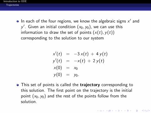
In each of the four regions, we know the algebraic signs x ′ andy ′. Given an initial condition (x0, y0), we can use thisinformation to draw the set of points (x(t), y(t))corresponding to the solution to our system

x ′(t) = −3 x(t) + 4 y(t)

y ′(t) = −x(t) + 2 y(t)

x(0) = x0

y(0) = y0.

This set of points is called the trajectory corresponding tothis solution. The first point on the trajectory is the initialpoint (x0, y0) and the rest of the points follow from thesolution.

Introduction to ODE

Trajectories

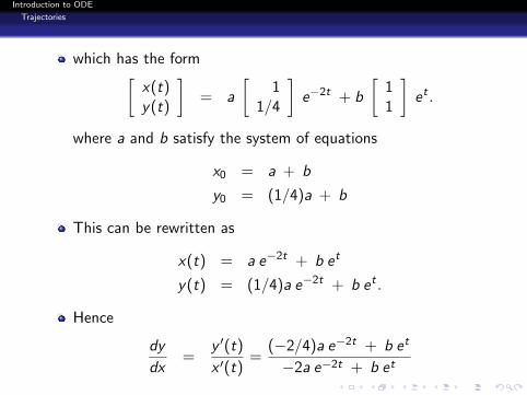
which has the form[x(t)y(t)

]= a

[1

1/4

]e−2t + b

[11

]et .

where a and b satisfy the system of equations

x0 = a + b

y0 = (1/4)a + b

This can be rewritten as

x(t) = a e−2t + b et

y(t) = (1/4)a e−2t + b et .

Hence

dy

dx=

y ′(t)

x ′(t)=

(−2/4)a e−2t + b et

−2a e−2t + b et

Introduction to ODE

Trajectories

When t is large, as long as b is not zero, the terms involvinge−2t are negligible and so we have

dy

dx=

y ′(t)

x ′(t)≈ b et

b et≈ the slope of E2.

Hence, when t is large, the slopes of the trajectory approach1, the slope of E2. So, we conclude for large t, for b not zero,the trajectory either parallels the E2 line or approaches itasymptotically.For an initial condition on the E1 line, b is zero and

dy

dx=

y ′(t)

x ′(t)=

(−2/4)a e−2t

−2a e−2t=

1

4= the slope of E1.

In this case,

x(t) = a e−2t , y(t) = (1/4)a e−2t ⇒ (x(t), y(t))→ (0, 0).

along the E1 line.

Introduction to ODE

Trajectories

Conclusions:

Given an IC which does not lie on E1 or E2, (x(t), y(t))approaches E2 as t gets large. Since the second eigenvalue is+1, (x(t), y(t)) moves away from the origin (0, 0) as tincreases. Note +1 is the dominant eigenvalue and thesetrajectories move toward the E2 line.

Given an IC which starts on E2, (x(t), y(t)) are always on theE2 line and since the second eigenvalue is 1, (x(t), y(t))moves outward from (0, 0) along the E2 line as t gets large.

We need to study the trajectories in the various derivative signregions next.

Introduction to ODE

Phase Plane Examples

Let’s summarize what we have said about trajectories again.

In each of the four regions, we know the algebraic signs x ′ andy ′. Given an initial condition (x0, y0), we can use thisinformation to draw the set of points (x(t), y(t))corresponding to the solution to our system

x ′(t) = −3 x(t) + 4 y(t)

y ′(t) = −x(t) + 2 y(t)

x(0) = x0

y(0) = y0.

This set of points is called the trajectory corresponding tothis solution. The first point on the trajectory is the initialpoint (x0, y0) and the rest of the points follow from thesolution.

Introduction to ODE


which has the form[x(t)y(t)

]= a

[1

1/4

]e−2t + b

[11

]et .

where a and b satisfy the system of equations

x0 = a + b

y0 = (1/4)a + b

This can be rewritten as

x(t) = a e−2t + b et

y(t) = (1/4)a e−2t + b et .

Hence

dy

dx=

y ′(t)

x ′(t)=

(−2/4)a e−2t + b et

−2a e−2t + b et

Introduction to ODE


When t is large, as long as b is not zero, the terms involvinge−2t are negligible and so we have

dy

dx=

y ′(t)

x ′(t)≈ b et

b et≈ the slope of E2.

Hence, when t is large, the slopes of the trajectory approach1, the slope of E2. So, we conclude for large t, for b not zero,the trajectory either parallels the E2 line or approaches itasymptotically.For an initial condition on the E1 line, b is zero and

dy

dx=

y ′(t)

x ′(t)=

(−2/4)a e−2t

−2a e−2t=

1

4= the slope of E1.

In this case,

x(t) = a e−2t , y(t) = (1/4)a e−2t ⇒ (x(t), y(t))→ (0, 0).

along the E1 line.

Introduction to ODE


Conclusions:

Given an IC which does not lie on E1 or E2, (x(t), y(t))approaches E2 as t gets large. Since the second eigenvalue is+1, (x(t), y(t)) moves away from the origin (0, 0) as tincreases. Note +1 is the dominant eigenvalue and thesetrajectories move toward the E2 line.

Given an IC which starts on E2, (x(t), y(t)) are always on theE2 line and since the second eigenvalue is 1, (x(t), y(t))moves outward from (0, 0) along the E2 line as t gets large.

Now let’s study the trajectories in each sign region.

Introduction to ODE

(+,+) Region

ICs start in the (+,+) Region: ICs are black dots.

x ′ = 0

x ′ = 0

y ′ = 0

y ′ = 0

~E 2

~E 2

~E 1

~E 1

(+,+)

(−,+)

(−,−)

(+,−)

ICs in the (+,+)region have x ′ > 0and y ′ > 0. Sothe trajectory wedraw must havex and y bothincreasing. Wedraw their con-cavity so that thesolution we drawdoes not havecorners. Notethe trajectoriesapproach the E2

line.

Introduction to ODE

(+,+) Region

We drew the trajectories in the last figure so that they didn’t cross.Here is why.

Consider the trajectories shown in next figure. These twotrajectories cross at some point.

The two trajectories correspond to different initial conditionswhich means that the a and b associated with them will bedifferent.

Further, these initial conditions don’t start on eigenvector ~E 1

or eigenvector ~E 2, so the a and b values for both trajectorieswill be non zero.

Introduction to ODE

(+,+) Region

x ′ = 0

x ′ = 0

y ′ = 0

y ′ = 0

~E 2

~E 2

~E 1

~E 1

(+,+)

(−,+)

(−,−)

(+,−)

In this figure,we show twotrajectories inthe (+,+) regionthat cross. Weshow this isnot possible inthe argumentthat follows thisfigure.

Introduction to ODE

(+,+) Region

If we label these trajectories by (x1, y1) and (x2, y2), we see

x1(t) = a1 e−2t + b1 e

t

y1(t) = (1/4)a1 e−2t + b1 e

t .

and

x2(t) = a2 e−2t + b2 e

t

y2(t) = (1/4)a2 e−2t + b2 e

t .

Since we assume they cross, there has to be a time point, t∗,so that (x1(t∗), y1(t∗)) and (x2(t∗), y2(t∗)) match.

Introduction to ODE

(+,+) Region

Now in vector notation, we know[x1(t)y1(t)

]= a1

[114

]e−2t + b1

[11

]et ,[

x2(t)y2(t)

]= a2

[114

]e−2t + b2

[11

]et .

Setting these two equal at t∗, then gives

a1

[114

]e−2t

∗+ b1

[11

]et

∗= a2

[114

]e−2t

∗+ b2

[11

]et

∗.

Introduction to ODE

(+,+) Region

For convenience, let et∗

= U and e−2t∗

= V . Then, werewrite as

a1

[114

]V + b1

[11

]U = a2

[114

]V + b2

[11

]U.

Next, we can combine like vectors to find

(a1 − a2)V

[114

]= (b2 − b1)U

[11

].

No matter what a1, a2, b1 and b2 are this says

E1 =

[114

]= a multiple of

[11

]= E2.

This is not possible, so the trajectories can’t cross. We can dothis analysis for trajectories that start in the other (+,−),(−,+) or a (−,−) regions also.A similar argument shows that a trajectory can’t cross aneigenvector line as if so, the same argument says ~E 1 is amultiple of ~E 2, which it is not.

Introduction to ODE

(−,+) Region

x ′ = 0

x ′ = 0

y ′ = 0

y ′ = 0

~E 2

~E 2

~E 1

~E 1

(+,+)

(−,+)

(−,−)(+,−)

Trajectories thatstart in the (−,+)region have x ′ <0 and y ′ > 0so x decreases andy increases. Thetrajectories moveinto the (+,+) re-gion and althoughthey can’t cross inthat region, it isdifficult to drawthem!

Introduction to ODE

(−,−)Region

x ′ = 0

x ′ = 0

y ′ = 0

y ′ = 0

~E 2

~E 2

~E 1

~E 1

(+,+)

(−,+)

(−,−)(+,−)

Trajectories inthe (−,−) regionhave x ′ < 0 andy ′ < 0 so both xand y decrease.We show threetrajectories; oneis a trajectorythat moves fromthe (−,−) re-gion through the(−,+) regionto the (+,+)region. Note allthe trajectoriesmoves towardsthe E2 line.

Introduction to ODE

(−,−)Region

x ′ = 0

y ′ = 0

~E 2

~E 1

(+,+)

(−,+)

(−,−)

A magnifiedtrajectory thatmoves from the(−,−) regionthrough the(−,+) region tothe (+,+) region.It approaches theE2 line.

Introduction to ODE

(+,−) Region

x ′ = 0

x ′ = 0

y ′ = 0

y ′ = 0

~E 2

~E 2

~E 1

~E 1

(+,+)

(−,+)

(−,−)(+,−)

Trajectories inthe (+,−) regionhave x ′ > 0and y ′ < 0 so xincreases and ydecreases. Thesetrajectories moveinto the (−,−)region and ap-proaches the E2

line.

Introduction to ODE

Combining All The Regions

x ′ = 0

x ′ = 0

y ′ = 0

y ′ = 0

~E 2

~E 2

~E 1

~E 1

(+,+)

(−,+)

(−,−)(+,−)

We show trajec-tories in all fourregions here. Wealso show thetrajectories thatstart on the E1

line and movetowards (0, 0)along that line andthe trajectoriesthat start on theE2 line that moveoutwards from(0, 0) along thatline.

Figure: Trajectories In All Regions

Introduction to ODE

Conclusions

We can do this for the three cases:

One eigenvalue negative and one eigenvalue positive: exampler1 = −2 and r2 = 1 which we have just completed.

Both eigenvalues negative: example r1 = −2 and r2 = −1which we have not done.

Both eigenvalues positive: example r1 = 1 and r2 = 2 whichwe have not done.

In each case, we have two eigenvectors E1 and E2. The waywe label our eigenvalues will always make most trajectoriesapproach the E2 line as t increases because r2 is always thelargest eigenvalue.

Introduction to ODE

Conclusions

Case: One negative eigenvalue and one positive eigenvalue. Thepositive one is the dominant one: example, r1 = −2 and r2 = 1 sothe dominant eigenvalue is r2 = 1.

Trajectories that start on the E1 line go towards (0, 0) alongthat line.

Trajectories that start on the E2 line move outward along thatline.

All other ICs give trajectories that move outward from (0, 0)and approach the dominant eigenvector line, the E2 line as tincreases.

The (+,+), (+,−), (−,+) and (−.−) regions tells us thedetails of how this is done. We find these regions using thenullcline analysis.

Introduction to ODE

Conclusions

Case: Two negative eigenvalues. The least negative one is thedominant one: example, r1 = −2 and r2 = −1 so the dominanteigenvalue is r2 = −1.


Trajectories that start on the E2 line go towards from (0, 0)along that line.

All other ICs give trajectories move towards (0, 0) andapproach the dominant eigenvector line, the E2 line as tincreases.


Introduction to ODE

Conclusions

Case: Two positive eigenvalues. The positive one is the dominantone: example, r1 = 2 and r2 = 3 so the dominant eigenvalue isr2 = 3.



All other ICs give trajectories move outward and approach thedominant eigenvector line, the E2 line as t increases. Thiscase where both eigenvalues are positive is the hardest one todraw and many times these trajectories become parallel to thedominant line rather than approaching it.


Introduction to ODE

Example

Here is a worked out example done by hand.

Introduction to ODE

Example

Introduction to ODE

Examples

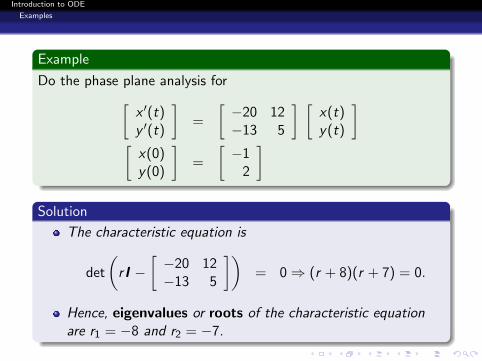
Example

Do the phase plane analysis for[x ′(t)y ′(t)

]=

[−20 12−13 5

] [x(t)y(t)

][

x(0)y(0)

]=

[−1

2

]

Solution

The characteristic equation is

det

(r I −

[−20 12−13 5

])= 0⇒ (r + 8)(r + 7) = 0.

Hence, eigenvalues or roots of the characteristic equationare r1 = −8 and r2 = −7.

Introduction to ODE

Examples

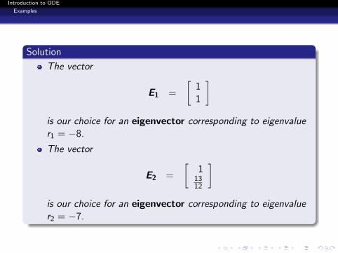
Solution

The vector

E1 =

[11

]is our choice for an eigenvector corresponding to eigenvaluer1 = −8.

The vector

E2 =

[1

1312


Introduction to ODE

Examples

Solution

Since both eigenvalues are negative we have r2 = −7 is thedominant one.



All other ICs give trajectories that move towards (0, 0) andapproach the dominant eigenvector line, the E2 line as tincreases.

The (+,+), (+,−), (−,+) and (−.−) regions tells us thedetails of how this is done. We find these regions using thenullcline analysis. Here x ′ = 0 gives −20x + 12y = 0 ory = 20/12x while y ′ = 0 gives −13x + 5y = 0 or y = 13/5x .

Introduction to ODE

Examples

Solution

The phase plane plot here is generated by Matlab. Matlab doesnot necessarily return the eigenvalues in the order we do by hand.So the E1 and E2 can be reversed in the figure.

Introduction to ODE

Examples

Example


]=

[4 9−1 −6

] [x(t)y(t)

][

x(0)y(0)

]=

[4−2

]

Solution


det

(r I −

[4 9−1 −6

])= 0⇒ (r + 5)(r − 3) = 0.

Hence, eigenvalues or roots of the characteristic equationare r1 = −5 and r2 = 3.

Introduction to ODE

Examples

Solution

The vector

E1 =

[1−1


The vector

E2 =

[1−1

9

]is our choice for an eigenvector corresponding to eigenvaluer2 = 3.

Introduction to ODE

Examples

Solution

Since one eigenvalue is positive and one is negative, we haver2 = 3 is the dominant one.


Trajectories that start on the E2 line move outward from(0, 0) along that line.


The (+,+), (+,−), (−,+) and (−.−) regions tells us thedetails of how this is done. We find these regions using thenullcline analysis. Here x ′ = 0 gives 4x + 9y = 0 ory = −4/9x while y ′ = 0 gives −x − 6y = 0 or y = −1/6x .

Introduction to ODE

Examples

Solution

The phase plane plot of this example is shown here. Matlab doesnot necessarily return the eigenvalues in the order we do by hand.So the E1 and E2 can be reversed in the figure.

Introduction to ODE

Examples

Solution

More trajectories!

Introduction to ODE

Examples

Solution

Even more trajectories!

Introduction to ODE

Examples

Example


]=

[4 −23 −1

] [x(t)y(t)

][

x(0)y(0)

]=

[14−22

]

Solution


det

(r I −

[4 −23 −1

])= 0⇒ (r − 1)(r − 2) = 0.

Hence, eigenvalues or roots of the characteristic equationare r1 = 1 and r2 = 2.

Introduction to ODE

Examples

Solution

The vector

E1 =

[132


The vector

E2 =

[11


Introduction to ODE

Examples

Solution

Since both eigenvalues are positive, the larger one, r2 = 2, isthe dominant one.




The (+,+), (+,−), (−,+) and (−.−) regions tells us thedetails of how this is done. We find these regions using thenullcline analysis. Here x ′ = 0 gives 4x − 2y = 0 or y = 2xwhile y ′ = 0 gives 3x − y = 0 or y = 3x .

Introduction to ODE

Examples

Solution

The phase plane plot of this example is shown here. Matlab doesnot necessarily return the eigenvalues in the order we do by hand.HereE1 and E2 are reversed in the figure.

Introduction to ODE

Examples

Solution

More trajectories!

Introduction to ODE

Examples

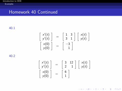
Homework 40

Find the characteristic equation

Find the general solution

Solve the IVP

On the same x − y graph,1 draw the x ′ = 0 line2 draw the y ′ = 0 line3 draw the eigenvector one line4 draw the eigenvector two line5 divide the x − y into four regions corresponding to the

algebraic signs of x ′ and y ′

6 draw the trajectories of enough solutions for various initialconditions to create the phase plane portrait

Introduction to ODE

Examples

Homework 40 Continued

40.1 [x ′(t)y ′(t)

]=

[1 33 1

] [x(t)y(t)

][

x(0)y(0)

]=

[−3

1

]40.2 [

x ′(t)y ′(t)

]=

[3 122 1

] [x(t)y(t)

][

x(0)y(0)

]=

[61

]

Introduction to ODE

Examples

40.3 [x ′(t)y ′(t)

]=

[−1 1−2 −4

] [x(t)y(t)

][

x(0)y(0)

]=

[38

]40.4 [

x ′(t)y ′(t)

]=

[3 4−7 −8

] [x(t)y(t)

][

x(0)y(0)

]=

[−2

4

]40.5 [

x ′(t)y ′(t)

]=

[−1 1−3 −5

] [x(t)y(t)

][

x(0)y(0)

]=

[2−4

]

qualitative analysis of linear systems of ode: phase...

Documents