Reservoir Engineering 2 Course (1st Ed.)

1. mathematical Water Influx models;A. The van Everdingen-Hurst Unsteady-State Model

a. Edge-Water DriveI. computational steps for We at successive intervals

1. mathematical Water Influx models;A. The van Everdingen-Hurst Unsteady-State Model

bottom-Water Drive

B. The Carter-Tracy Water Influx Model

C. Fetkovich’s Method

bottom-water drive occurrence

The van Everdingen-Hurst solution to the radial diffusivity equation is considered the most rigorous aquifer influx model to date. The proposed solution technique, however,

is not adequate to describe the vertical water encroachment in a bottom-water-drive system.

Coats (1962) presented a mathematical model that takes into account the vertical flow effects from bottom-water aquifers. He correctly noted that in many cases reservoirs

are situated on top of an aquifer with a continuous horizontal interface between the reservoir fluid and the aquifer water and with a significant aquifer thickness. He stated that in such situations

significant bottom-water drive would occur.

Spring14 H. AlamiNia Reservoir Engineering 2 Course (1st Ed.) 5

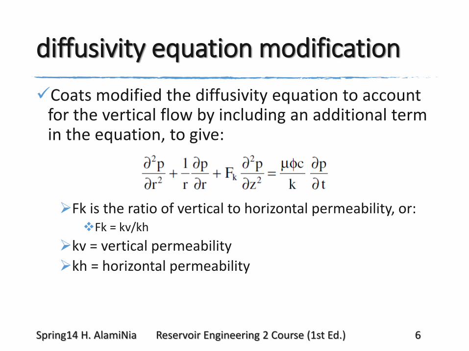
diffusivity equation modification

Coats modified the diffusivity equation to account for the vertical flow by including an additional term in the equation, to give:

Fk is the ratio of vertical to horizontal permeability, or:Fk = kv/kh

kv = vertical permeability

kh = horizontal permeability

Spring14 H. AlamiNia Reservoir Engineering 2 Course (1st Ed.) 6

Allard and Chen correlation parameters; bottom-Water DriveAllard and Chen (1988) suggested that it is possible

to derive a general solution that is applicable to a variety of systems by the solution to the Equation in terms of the dimensionless time tD,

dimensionless radius rD, and

a newly introduced dimensionless variable zD.

zD = dimensionless vertical distance

h = aquifer thickness, ft

Spring14 H. AlamiNia Reservoir Engineering 2 Course (1st Ed.) 7

Allard and Chen correlation; bottom-Water Drive Allen and Chen used a numerical model to solve

the Equation. The authors developed a solution to the bottom-water influx that is comparable in form with that of van Everdingen and Hurst.They defined the water influx constant B identical to

previous Equation, orNotice that B does not include the encroachment angle θ.

The actual values of WeD are different from those of the van Everdingen-Hurst model because WeD for the bottom-water drive is also a function of

the vertical permeability.

Allard and Chen tabulated the values of WeD as a function of rD, tD, and zD.

Spring14 H. AlamiNia Reservoir Engineering 2 Course (1st Ed.) 8

WeD (the bottom-water drive)for Infinite Aquifer

Spring14 H. AlamiNia Reservoir Engineering 2 Course (1st Ed.) 9

WeD (the bottom-water drive)for finite Aquifer

Spring14 H. AlamiNia Reservoir Engineering 2 Course (1st Ed.) 10

Van Everdingen-Hurst methodology vs. Carter and Tracy methodologyVan Everdingen-Hurst methodology provides the

exact solution to the radial diffusivity equation and therefore is considered the correct technique for calculating water influx. However, because superposition of solutions is required,

their method involves tedious calculations. To reduce the complexity of water influx calculations,

Carter and Tracy (1960) proposed a calculation technique that does not require superposition and allows direct calculation of water influx.

It should be noted that the Carter-Tracy method is not an exact solution to the diffusivity equation and should be considered an approximation.

Spring14 H. AlamiNia Reservoir Engineering 2 Course (1st Ed.) 12

Carter-Tracy; Calculation of the cumulative water influx at any timeThe primary difference between

the Carter-Tracy technique and the van Everdingen-Hurst technique is that the Carter-Tracy technique assumes

constant water influx rates over each finite time interval. Using the Carter-Tracy technique, the cumulative water influx at

any time, tn, can be calculated directly from the previous value obtained at tn − 1, or:

B = the van Everdingen-Hurst water influx constanttD = the dimensionless time as defined n (n-1) = refers to the current (previous) time stepΔpn = total pressure drop, pi − pn, psi pD (p′D)= dimensionless pressure (derivative)

Spring14 H. AlamiNia Reservoir Engineering 2 Course (1st Ed.) 13

Values of the dimensionless pressure pDValues of the dimensionless pressure pD as a

function of tD and rD are tabulated in Chapter 6 (Handbook of reservoir engineering, T, Ahmed).

In addition to the curve-fit equations (for tD<0.01, 25<tD, tD>100, 0.02<tD<1000), Edwardson and coauthors (1962) developed the following approximation of pD for an infinite-acting aquifer.

Spring14 H. AlamiNia Reservoir Engineering 2 Course (1st Ed.) 14

The dimensionless pressure derivative

The dimensionless pressure derivative can then be approximated by

The following approximation could also be used between tD > 100:

with the derivative as given by:

Spring14 H. AlamiNia Reservoir Engineering 2 Course (1st Ed.) 15

Van Everdingen-Hurst methodology vs. Fetkovich methodologyFetkovich (1971) developed a method of

describing the approximate water influx behavior of a finite aquifer for radial and linear geometries. In many cases, the results of this model

closely match those determined using the van Everdingen-Hurst approach.

The Fetkovich theory is much simpler, and, like the Carter-Tracy technique, this method does not require the use of superposition.

Hence, the application is much easier, and this method is also often utilized in numerical simulation models.

Spring14 H. AlamiNia Reservoir Engineering 2 Course (1st Ed.) 18

Fetkovich’s model Introduction

Fetkovich’s model is based on the premise that the productivity index concept will adequately describe water influx from a finite aquifer into a hydrocarbon reservoir. That is, the water influx rate is directly proportional

to the pressure drop between the average aquifer pressure and the pressure at the reservoir-aquifer boundary.

The method neglects the effects of any transient period. Thus, in cases where

pressures are changing rapidly at the aquifer/reservoir interface, predicted results may differ somewhat from the more rigorous van Everdingen-Hurst or Carter-Tracy approaches.

In many cases, however, pressure changes at the waterfront are gradual and this method offers an excellent approximation to the two methods discussed above.

Spring14 H. AlamiNia Reservoir Engineering 2 Course (1st Ed.) 19

Fetkovich’s model approach

This approach begins with two simple equations. The first is the productivity index (PI) equation for the aquifer, which is analogous to the PI equation used to describe an oil or gas well:

ew = water influx rate from aquifer, bbl/day

J = productivity index for the aquifer, bbl/day/psi

–pa = average aquifer pressure, psi

pr = inner aquifer boundary pressure, psi

Spring14 H. AlamiNia Reservoir Engineering 2 Course (1st Ed.) 20

Fetkovich’s model approach (Cont.)

The second equation is an aquifer material balance equation for a constant compressibility, which states that the amount of pressure depletion in

the aquifer is directly proportional to the amount of water influx from the aquifer, or:

Wi = initial volume of water in the aquifer, bbl

ct = total aquifer compressibility, cw + cf, psi−1

pi = initial pressure of the aquifer, psi

f = θ/360

Spring14 H. AlamiNia Reservoir Engineering 2 Course (1st Ed.) 21

average aquifer pressure determinationThe maximum possible water influx occurs if pa = 0,

or:

Combining the Equations gives:

The Equation provides a simple expression to determine the average aquifer pressure p–a

after removing We bbl of water from the aquifer to the reservoir, i.e., cumulative water influx.

Differentiating with respect to time gives:

Spring14 H. AlamiNia Reservoir Engineering 2 Course (1st Ed.) 22

cumulative water influx

Fetkovich combined the differentiated Equation with the PI equation and integrated to give the following form:

We = cumulative water influx, bbl

pr = reservoir pressure, i.e., pressure at the oil- or gas-water contact

t = time, days

Spring14 H. AlamiNia Reservoir Engineering 2 Course (1st Ed.) 23

The productivity index J

The productivity index J used in the calculation is a function of the geometry of the aquifer. Fetkovich calculated the productivity index from Darcy’s

equation for bounded aquifers.

Lee and Watten barger (1996) pointed out that Fetkovich’s method can be extended to infinite acting aquifers by requiring that

the ratio of water influx rate to pressure drop be approximately constant throughout the productive life of the reservoir.

Spring14 H. AlamiNia Reservoir Engineering 2 Course (1st Ed.) 24

The productivity index J formulation

w = width of the linear aquifer

L = length of the linear aquifer

rD = dimensionless radius, ra/re

k = permeability of the aquifer, md

t = time, days

θ = encroachment angle

h = thickness of the aquifer

f = θ/360

Spring14 H. AlamiNia Reservoir Engineering 2 Course (1st Ed.) 25

Summary of the methodology of using Fetkovich’s modelThe following steps describe the methodology of

using Fetkovich’s model in predicting the cumulative water influx.Step 1. Calculate initial volume of water in the aquifer

Step 2. Calculate the maximum possible water influx Wei

Step 3. Calculate the productivity index J based on the boundary conditions and aquifer geometry.

Step 4. Calculate the incremental water influx (ΔWe)n from the aquifer during the nth time interval

Step 5. Calculate the cumulative (total) water influx at the end of any time period

Spring14 H. AlamiNia Reservoir Engineering 2 Course (1st Ed.) 26

1. Ahmed, T. (2010). Reservoir engineering handbook (Gulf Professional Publishing). Chapter 10

1. Primary Recovery MechanismsA. Rock and Liquid Expansion Drive Mechanism

B. The Depletion-Drive Mechanism

C. Gas-Cap Drivea. Gas-Cap Drive; Recovery