python-based geoprocessing tools for visualizing ... · python-based geoprocessing tools for...
TRANSCRIPT
Python-based geoprocessing tools for visualizing subsurface geology A capstone project report
Jesse Schaefer, Drew Schwitters, Martin Weiser
University of Washington, Geography 569 GIS Workshop August 17th, 2018 Report submitted to GeoMapNW

EXECUTIVE SUMMARY
The Pacific Northwest Center for Geologic Mapping Studies (GeoMapNW) is a Seattle-based
collaborative research center established by the USGS in 1998. The organization was founded to
help create disaster-resilient cities by providing state of the art geologic data to support geologic
hazard mitigation projects and inform land use decisions in the Puget Lowland region. A major
accomplishment of GeoMapNW was the creation and continued maintenance of a database
containing subsurface geologic information compiled primarily from geotechnical boring logs,
water well logs, and direct measurements (known collectively as geological explorations). To
date, over 100,000 explorations and their associated attributes have been added to this database.
In order to visually display the information contained in this database for the production of
geologic maps and related information products, a series of tools were developed in VBA to
create cross section views of these explorations and the overlying surface elevation profile. These
tools rely on currently outdated and unsupported software and were built to interact with
database architecture abandoned by GeoMapNW. Because of this, the organization no longer had
the ability to visualize subsurface geology, and commercially available cross section tools could
not be used due to prohibitive cost and incompatibility with existing database architecture.
To address this loss of geovisualization ability, GeoMapNW submitted a project proposal to the
2018 University of Washington Masters of GIS for Sustainability Management capstone program
to solicit the development of a tool to automate the creation of geologic cross sections. The
authors accepted the proposal and began developing several Python-based geoprocessing tools
intended for use in ArcMap. These tools borrow heavily from open-source Python scripts written
by Evan Thoms of the USGS, though they are extensively modified to address key desired
software capabilities identified by GeoMapNW during initial project scoping. Following several
weeks of development, the tools were completed and delivered to GeoMapNW in the form of an
ArcGIS toolbox (.tbx) with supporting materials including help documentation and relevant layer
files used for the application of symbology.
Tool capabilities include returning a 2D cross section view of stick logs of selected GeoMapNW
explorations with an overlying surface elevation profile. Each stick log displays major material
composition, visualized for each subsurface layer. The user may also specify a vertical and
horizontal exaggeration for the output, display the depth of groundwater encountered in each
exploration, display the density of each layer, apply symbology as desired, and export the end
result to a graphic file format for further editing.
Initial user testing of the tools was successful. Dr. Kathy Troost, Director of GeoMapNW, stated
that the tools will be used with near immediacy on a project to map the depth to bedrock in the
Seattle area and expects that the tools will allow for the visual identification of vertical offsets in
the bedrock that may assist in accurately locating the Seattle Fault.
The following report presents an in-depth explanation of the need for these cross section tools,
the processes and methodology involved in their development, and concluding examinations of
their technical capabilities with suggestions for further refinement.

ii
TABLE OF CONTENTS
1. BACKGROUND AND PROBLEM STATEMENT 1
1.1 Background .............................................................................................................................................................. 1
1.2 Project Goal and Problem Statement ....................................................................................................................... 4
1.3 This Report .............................................................................................................................................................. 5
2. SYSTEM RESOURCE REQUIREMENTS 6
2.1 Data Resource Requirements ................................................................................................................................... 6
2.2 Software Resource Requirements ............................................................................................................................ 8
2.3 Hardware Resource Requirements ........................................................................................................................... 9
2.4 Personnel Resource Requirements......................................................................................................................... 10
2.5 Institutional Resource Requirements ..................................................................................................................... 11
3. BUSINESS CASE EVALUATION 12
3.1 Benefits of Commissioning a Student-Developed Geologic Cross Section Tool .................................................. 12
3.2 Costs of Commissioning a Student-Developed Geologic Cross Section Tool ...................................................... 14
3.3 Benefit-Cost Analysis: Cost savings vs. Alternative solutions .............................................................................. 16
3.4 Benefit-Cost Analysis Conclusions ....................................................................................................................... 18
4. DATA DEVELOPMENT 20
4.1 Data Acquisition .................................................................................................................................................... 20
4.2 Data Quality Issues ................................................................................................................................................ 20
4.3 Future Data Preparation ......................................................................................................................................... 21
4.4 Shared Group Challenges ...................................................................................................................................... 22
4.5 Database Schema Specifications ........................................................................................................................... 22
4.6 Description of Attribute Table Information ........................................................................................................... 23
4.7 Content Metadata Descriptions .............................................................................................................................. 24
5. WORKFLOW IMPLEMENTATION 26
5.1 Determination of Deliverables ............................................................................................................................... 26
5.2 Refining the Workflow Processing Plan ................................................................................................................ 27
5.3 Actual Workflow Implementation ......................................................................................................................... 28
5.4 Concluding the Workflow Implementation ........................................................................................................... 35
6. RESULTS 36
6.1 Tool Results ........................................................................................................................................................... 36
6.2 User Testing Results and GeoMapNW Use Viability ........................................................................................... 43
7. CONCLUSIONS AND RECOMMENDATIONS 45
7.1 Conclusions Regarding Tool Suitability and Client Adoption .............................................................................. 45
7.2 Conclusions Regarding Tool Capabilities Relating to Need-To-Know Questions ................................................ 45
7.3 Recommendations for Further Development ......................................................................................................... 47

iii
8. REFERENCES 51
9. TECHNICAL APPENDICES 52
Appendix A: Data Design Tables ................................................................................................................................ 52
Appendix B: Python Scripts. ...................................................................................................................................... 61
Appendix C. Toolbox Instructions Document ............................................................................................................. 75
Appendix D. “Tool parameter documentation” file ..................................................................................................... 92
LIST OF TABLES
Table 1. Need to know questions……………………………………………………………………………………… 5
Table 2. Selection of tools and python modules called in toolbox scripts…………………………………………….. 9
Table 3. Team members and project role..……………………………………………………………………………10
Table 4. Benefit categories……………………………………………………………………………………………12
Table 5. Estimated cost savings……………………………………………………………………………………… 17
Table 6. Estimated expenditures……………………………………………………………………………………... 18
Table 7. Database schema specifications…………………………………………………………………………….. 23
Table 8. Attribute table specifications……………………………………………………………………………….. 24
Table 9. Metadata descriptions for rasters, feature classes, tables and tools………………………………………… 25
Table 10. Schema specifications……………………………………………………………………………………... 52
Table 11. Attribute table specifications……………………………………………………………………………… 53
Table 12. Metadata descriptions……………………………………………………………………………………... 59
LIST OF FIGURES
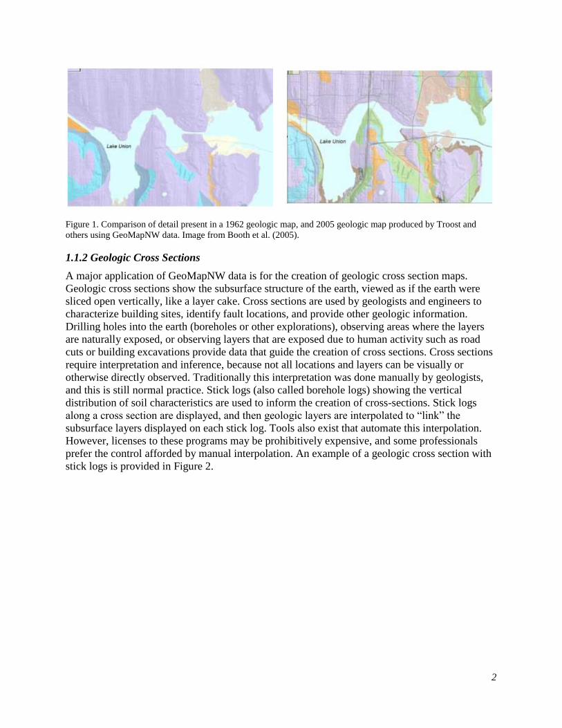
Figure 1. Comparison of detail present in a 1962 geologic map, and 2005 geologic map……………………………. 2
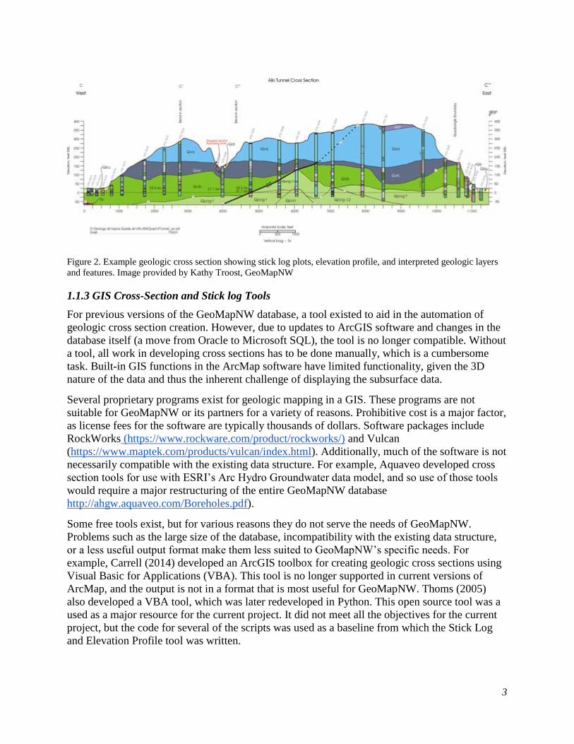
Figure 2. Example geologic cross section showing stick log plots, elevation profile, and interpreted geologic layers
and features……………………………………………………………………………………………………… 3
Figure 3. An entity-relationship diagram of the relevant geomapnw database elements……………………………... 7
Figure 4. Operations flow diagram of basic data inputs and outputs for the three developed tools…………………... 8
Figure 5. Total cost savings vs. Cost of alternative solutions………………………………………………………... 18
Figure 6. Output from a VBA tool developed for GeoMapNW……………………………………………………... 26
Figure 7. Outputs from Evan Thoms’ geoprocessing tools………………………………………………………….. 28
Figure 8. A surface profile and stick log with an unknown spatial reference………………………………………...30
Figure 9. Operations flow diagram demonstrating the code block used to create the surface elevation profile line... 31
Figure 10. Operations flow diagram demonstrating the code block used to create stick logs……………………….. 32
Figure 11. Operations flow diagram demonstrating the code block for the location of groundwater……………….. 33
Figure 12. Operations flow diagram for the symbology script………………………………………………………. 34
Figure 13. Operations flow diagram for the export to graphic script…………………………………………………35

iv
Figure 14. Contents of the final deliverable sent to GeoMapNW viewed in arccatalog…………………………….. 35
Figure 15. A map containing displaying input data for the stick log and elevation profile tool may be run…………36
Figure 16. The user interface for the stick log and elevation profile tool……………………………………………. 37
Figure 17. Geoprocessing results from the stick log and elevation profile tool……………………………………... 38
Figure 18. Geoprocessing results from the stick log and elevation profile tool showing results from different vertical
and horizonatal exaggeration settings………………………………………………………………………….. 38
Figure 19. Output from the stick log and elevation profile tool for transect crossing the city of Kirkland..…………39
Figure 20. A legend included in the geologic cross section toolbox………………………………………………… 40
Figure 21. The user interface for the apply symbology tool with example parameters provided…………………….40
Figure 22. Results from the stick log and elevation profile tool after running the apply symbology tool…………... 41
Figure 23. The user interface for the apply symbology tool with example parameters provided…………………….42
Figure 24. Example output from the export to graphic tool…………………………………………………………..43
Figure 25. Final results from user testing using a connection to the online exploration database……………………44

1. BACKGROUND AND PROBLEM STATEMENT
The Pacific Northwest Center for Geologic Mapping Studies (GeoMapNW) is a Seattle-based
collaborative research program initiated in 1998. The program created and now maintains a
publicly available subsurface database containing geotechnical data for over 100,000 geologic
exploration points in the Seattle region. This data is used for increasing knowledge about
geologic conditions and hazards in order to inform land use decisions. GeoMapNW submitted a
project proposal to the 2018 University of Washington Masters in GIS for Sustainability
Management capstone program soliciting the development of a tool to partially automate the
creation of geologic cross section maps using GeoMapNW data.
1.1 Background
1.1.1 GeoMapNW
The Puget Sound Lowland is one of the most seismically active areas in the country, and is also
highly urbanized. Steep slopes, shallow water tables, and sandy deposits also increase the risk of
geologic hazards like landslides and soil liquefaction (Booth et al. 2005). In 1998, GeoMapNW
was established when Seattle was selected as one of several cities to participate in a U.S.
Geological Survey (USGS) program to help create disaster-resilient cities by providing state of
the art geologic data to support geologic hazard mitigation in the region. The program received
additional funding from the City of Seattle and King County. The University of Washington’s
Department Earth and Space Sciences hosts the program on its Seattle campus. The project’s
goals are to “acquire existing geologic data and create new geologic information; to conduct
geologic research and produce new geologic maps; and to support the wide variety of additional
research, hazard assessments, and land-use applications of other scientists, organizations, and
agencies throughout the region” (Booth et al. 2005).
In the program’s initial years, GeoMapNW compiled geotechnical data from geologic
explorations using a variety of sources and created a large publicly available database. This
database includes geotechnical information about subsurface geology including soil types,
subsurface layers, groundwater depth, and material density. These data can be used for
applications such as identifying fault locations; informing planning and development decisions;
and creating earthquake shaking scenarios, liquefaction, and landslide maps. The initial database
contained 35,000 exploration points; the current database has grown to over 100,000 points.
Using these data, GeoMapNW produced geologic maps for the region with much more detail and
higher quality than previously existing maps. The new maps have with about twice the spatial
resolution of previously existing maps. See Figure 1 for an example of old and new maps,
showing the enhanced detail in the new version. These maps are used for a variety of purposes
and by many users, but generally they provide information about geologic hazards and
susceptibility to events such as landslides and earthquakes. Findings from the maps and data
include evidence for faults and deformation, landslides, and the existence of organic-rich
deposits such as peat and lake deposits.
In 2010, after 12 years operating, the program lost funding. Currently, the program still exists on
the University of Washington campus but it has no paid staff. The Washington Department of
Natural Resources manages and distributes the data compiled by GeoMapNW. Efforts are being
made to refund the program and resume work at full capacity.
2
Figure 1. Comparison of detail present in a 1962 geologic map, and 2005 geologic map produced by Troost and
others using GeoMapNW data. Image from Booth et al. (2005).
1.1.2 Geologic Cross Sections
A major application of GeoMapNW data is for the creation of geologic cross section maps.
Geologic cross sections show the subsurface structure of the earth, viewed as if the earth were
sliced open vertically, like a layer cake. Cross sections are used by geologists and engineers to
characterize building sites, identify fault locations, and provide other geologic information.
Drilling holes into the earth (boreholes or other explorations), observing areas where the layers
are naturally exposed, or observing layers that are exposed due to human activity such as road
cuts or building excavations provide data that guide the creation of cross sections. Cross sections
require interpretation and inference, because not all locations and layers can be visually or
otherwise directly observed. Traditionally this interpretation was done manually by geologists,
and this is still normal practice. Stick logs (also called borehole logs) showing the vertical
distribution of soil characteristics are used to inform the creation of cross-sections. Stick logs
along a cross section are displayed, and then geologic layers are interpolated to “link” the
subsurface layers displayed on each stick log. Tools also exist that automate this interpolation.
However, licenses to these programs may be prohibitively expensive, and some professionals
prefer the control afforded by manual interpolation. An example of a geologic cross section with
stick logs is provided in Figure 2.
3
Figure 2. Example geologic cross section showing stick log plots, elevation profile, and interpreted geologic layers
and features. Image provided by Kathy Troost, GeoMapNW
1.1.3 GIS Cross-Section and Stick log Tools
For previous versions of the GeoMapNW database, a tool existed to aid in the automation of
geologic cross section creation. However, due to updates to ArcGIS software and changes in the
database itself (a move from Oracle to Microsoft SQL), the tool is no longer compatible. Without
a tool, all work in developing cross sections has to be done manually, which is a cumbersome
task. Built-in GIS functions in the ArcMap software have limited functionality, given the 3D
nature of the data and thus the inherent challenge of displaying the subsurface data.
Several proprietary programs exist for geologic mapping in a GIS. These programs are not
suitable for GeoMapNW or its partners for a variety of reasons. Prohibitive cost is a major factor,
as license fees for the software are typically thousands of dollars. Software packages include
RockWorks (https://www.rockware.com/product/rockworks/) and Vulcan
(https://www.maptek.com/products/vulcan/index.html). Additionally, much of the software is not
necessarily compatible with the existing data structure. For example, Aquaveo developed cross
section tools for use with ESRI’s Arc Hydro Groundwater data model, and so use of those tools
would require a major restructuring of the entire GeoMapNW database
http://ahgw.aquaveo.com/Boreholes.pdf).
Some free tools exist, but for various reasons they do not serve the needs of GeoMapNW.
Problems such as the large size of the database, incompatibility with the existing data structure,
or a less useful output format make them less suited to GeoMapNW’s specific needs. For
example, Carrell (2014) developed an ArcGIS toolbox for creating geologic cross sections using
Visual Basic for Applications (VBA). This tool is no longer supported in current versions of
ArcMap, and the output is not in a format that is most useful for GeoMapNW. Thoms (2005)
also developed a VBA tool, which was later redeveloped in Python. This open source tool was a
used as a major resource for the current project. It did not meet all the objectives for the current
project, but the code for several of the scripts was used as a baseline from which the Stick Log
and Elevation Profile tool was written.
4
1.2 Project Goal and Problem Statement
1.2.1 Project Goal
The goal of the project was to develop and Python-based ArcGIS custom tool for
geovisualization of stick logs along a user-selected cross section, showing a vertical plot of soil
types, densities, and groundwater locations for each point.
To meet project sponsor specifications, the tool needed to:
❏ Be compatible with the existing GeoMapNW data structure.
❏ Create a vertical plot (stick log) for a series of geologic exploration points along a cross
section line.
❏ Allow the user to input a cross section line and selected exploration points.
❏ Create a surface elevation profile for the cross section.
❏ Display the subsurface layers for each point including major material and material
density.
❏ Display the groundwater location for each point, if available.
❏ Create an editable legend using a borehole lithology key.
❏ Allow user specification of vertical and horizontal exaggeration.
❏ Create a graphic output that can be edited in a graphics program such as Adobe
Illustrator.
❏ Include documentation for users.
While most other tools and research focus on creating tools or data models that allow users to
work with cross-sections within a GIS software program, our focus differs slightly in that the
desired output is an editable graphic that will aid with the manual creation of cross sections. The
ArcGIS output will be exported to a file format supported by vector graphic editing software,
such as Adobe Illustrator. This exported file will be imported into the graphics software and
edited to include annotations and other modifications.
Development of the tool will facilitate and enhance the use of GeoMapNW subsurface geology
database. Through partial automation of the creation of geologic cross sections, accuracy of maps
will increase, as will the ease of data interpretation. By increasing geologic knowledge, the tool
will also contribute to improvements in disaster resilience. Project benefits are discussed in
further detail in section 3 of this report.
Based on the project goals, the following problem statement was developed:
How can we develop a tool for visualizing geologic data by automating the
creation of a surface profile and stick logs along a cross section line, using the
GeoMapNW database?

5
1.2.2 Project objectives
Based on the project goal, project objectives were developed. These are presented in Table 1 in
the form of “need to know questions.” The need to know questions are the basic questions that
needed to be answered in order to successfully develop a tool that will meet project goals. The
questions were developed by working backwards, starting with the specifications for outputs the
tool ultimately needed to generate, and assessing the information that would be necessary to
build each specification into the tool. Of course, in order to answer each question, many other
questions ultimately need to be answered first, but the need to know questions form a useful
framework for understanding the necessary problem-solving needed to approach the project.
Need to know questions:
What data points should be included in the cross section?
What is the location of each exploration and stick log?
What is the elevation profile along the cross section?
What is the groundwater depth?
What is the density of each layer?
What is the major material of each layer?
What is the depth of each layer?
How will appropriate symbology be applied?
How will the above be displayed visually in a graphic output?
Table 1. Need to know questions.
1.3 This Report
The following sections of this report document the process and results of the toolbox creation. In
System Resource Requirements, requirements for data, software, hardware, personnel, and
institutional requirements for the project are enumerated. In the Business Case Evaluation, a
cost-benefit analysis is presented arguing in favor of tool creation from a fiscal standpoint. In
Data Development, the GeoMapNW database structure and the data outputs of the tool are
described and discussed. In Workflow Implementation, the methods we undertook to develop the
tool are explained, as are technical aspects of script and tool creation. In Results, the final version
of the tool and its outputs are presented. Conclusions and Recommendations discusses the
usefulness and limitations of the final product, and recommendations for future work. Python
scripts, data design tables, tool parameter documentation, and a toolbox instructions document
are included as appendices.
6
2. SYSTEM RESOURCE REQUIREMENTS
This section discusses the necessary system resource requirements both in terms of those
necessary for project development, and those necessary for users of the produced tools. Data,
software, hardware, personnel, and institutional requirements are discussed.
2.1 Data Resource Requirements
Database design and the information environment are critical considerations when building a
custom tool. The existing or theoretical database and data models will influence the functionality,
features, interface, and outputs of the tool. In this project, we were tasked with creating a custom
tool using data compiled in an existing Microsoft SQL database. Our tool is specifically designed
to interface with the current database architecture. Because of this, data resource requirements
for our tool are dictated by the existing database structure (feature classes, rasters, relationship
classes, domains, etc.), and expected tool processing demands and outputs (geoprocessing steps,
and amount and format of output data).
2.1.1 GeoMapNW Existing Database
Due to the prior existence of the relevant database, completing the database design process
would constitute a serious duplication of effort. Nevertheless, it is beneficial to understand the
stages of developing a conceptual data model for the database design. Database design and
creation was a major accomplishment of the early work of the GeoMapNW program.
GeoMapNW identified the information products their organization sought to deliver (high
quality, high resolution geologic maps of the Puget Lowlands for assessing and identifying
seismic risk areas, landslide and liquefaction potential, groundwater resources, and hydrocarbon
potential in the urban corridor). They then reviewed existing data sources compared to data
requirements and identified key thematic layers and feature classes that would comprise the bulk
of the database (geologic explorations taken from public record, topographic and bathymetric
data, subsurface layer information, and related tables). Feature classes were detailed to create
data models. Subtypes, relationships, and domains were applied as appropriate. The database
design is discussed in further detail in section 4 of this report, Data Design.
Because the database design process had been completed prior to our project participation, our
project required working within the existing database. The most relevant data design factor is
that the exploration points are related to a subsurface layers table in a one to many relationship.
For each exploration point, many subsurface layers may exist, each with their own set of
attributes (depth, material, density, etc.), some of which are stored in separate related tables. The
objective of the tool is to develop a way to display this related data, which in a typical ArcMap
session is only accessible by manually clicking on a point with the identify tool to read attributes
from the related tables. Clearly, a tool that produces a visualization of this data will be a useful
improvement.
2.1.2 GeoMapNW Database Entity-Relationship Diagram
For project development, a subset of the main GeoMapNW database was downloaded to each
project member’s local drive. The database contains some basemap feature classes unnecessary
for tool development or display (streets, lakes, city boundaries, etc.). A simplified enity-
relationship diagram is displayed in Figure 3, showing only the feature classes, raster datasets,
and tables relevant to our tools. The Data_Points feature class, DEM raster, and

7
Subsurface_Layers table are required inputs. The Groundwater_WW table is necessary for
displaying groundwater depth. The other tables contain additional data related to each
exploration data point through a relationship class definition. Primary and foreign keys
(EXPLOR_ID field) and attribute fields relevant to the tools are included in the diagram. Many
other attributes exist but are omitted here for simplification. Further description of the data can
be found in section 4 of this report, Data Design.
Figure 3. An Entity-Relationship Diagram of the relevant GeoMapNW database elements.
It is useful to examine the relevant input layers and their key attributes as they will be applied by
the tool. A DEM raster is input for the display of an elevation profile along the user-provided
cross section line, and also determines the starting elevation of each exploration if the elevation
is not provided as an attribute. Data points from the ‘Data_Points’ layer are selected by the user
as inputs, and a stick log is created for each selected point. Groundwater and subsurface layer
tables with relationship classes to the ‘Data_Points’ layer are used to provide the attribute values
needed to create stick logs displaying the depth of each subsurface layer, the layer major material
type, material density, and groundwater level. A simple visualization of this process is presented
in Figure 4. The inputs and operational processes of the tool are discussed in further detail in
section 5 of this report, Workflow Implementation.

8
Figure 4. Operations Flow Diagram of basic data inputs and outputs for the three developed tools.
2.2 Software Resource Requirements
2.2.1 Software function capabilities
The scripts were written using Python version 2.7 and the tool was tested with ArcGIS versions
10.2 through 10.5.1. A license for the 3D analyst extension is required for tool operation. The
tools call Python (.py) files that are packaged within an ArcGIS toolbox. The Python module is
part of an ArcGIS Desktop install, so any ArcMap user with a 3D analyst license should be able
to execute the tool without additional software. The custom toolbox, containing three ArcGIS
custom script tools, is loaded into ArcToolbox and the tool is executed from ArcMap. An open
.mxd file with appropriate input data added to the data frame is necessary for the tool to function
(it cannot be run from the command line or from a Python IDE).
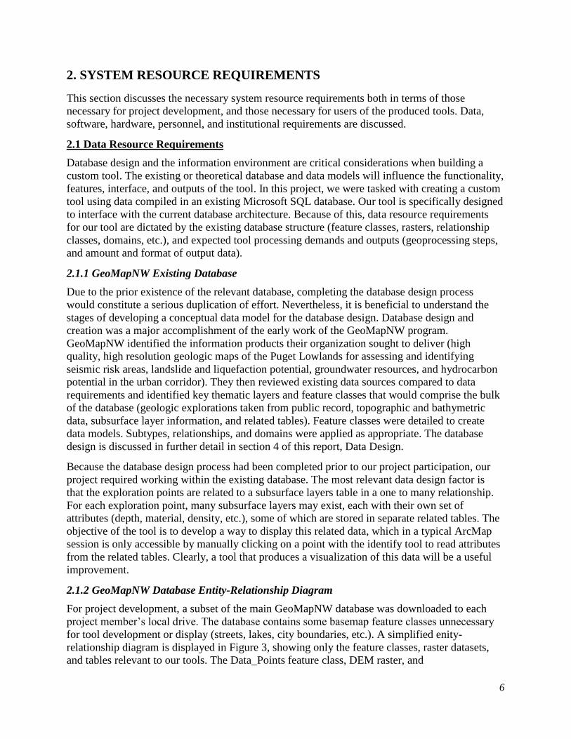
The scripts primarily utilize built-in ArcToolbox tools called through the Python Arcpy module,
as well as the os, sys, and traceback Python modules. From ArcToolbox, utilized tools include
many from the Data Management toolbox, as well as Data Access, Linear Referencing, Analysis,
Conversion, Mapping, and 3D Analyst tools. These tools are listed in Table 2.
Toolbox Tools/Modules
Data management Add Field
Calculate Field
Make Feature Layer
Add Join
Copy Features
Tool 1 inputs: Selected data points, Cross section line,
DEM
Tool 1: Stick Logs and Elevation Profile
Tool 1 outputs: Profile line, Stick
log lines, Stick log polygons FC Stick log groundwater
points
Tool 2: Apply Symbology
Tool 2 outputs: Symbolized stick
log polygons, groundwater
points, and density
Tool 3: Export to Graphic
Tool 3 output: Graphic file of
map layout view
Tool 2 additional
inputs: Major material, groundwater, and density layer files
9
List Fields
Apply Symbology from Layer
Feature to Point
Sort
Data Access
Search cursor
Update cursor
Sort management
Linear Referencing Create Routes
Locate Features Along Routes
Analysis Buffer
Mapping Add layer
List Data Frames
3D Analyst Interpolate Shape
Conversion
Export to PDF, AI, JPEG, etc
Python 2.7.13 Arcpy, os, sys, traceback modules
Table 2. Selection of tools and Python modules called in toolbox scripts.
If a tool user wants to edit the graphic file output, rather than working within the ArcMap
environment, vector graphics software will be necessary. The ideal software for this task is
Adobe Illustrator, as maps can be exported from ArcMap to Adobe Illustrator (.ai), and there is
more support for compatibility between programs than for some other software. However,
licenses to the Adobe Creative Cloud software are expensive and alternatives exist, for example
the open source program Inkscape. At the time of writing an individual Illustrator license was
about $20 per month, although educational discounts are available.
2.3 Hardware Resource Requirements
2.3.1 Data input storage requirements
Anticipated data input storage requirements are minimal and depend on the scale of a tool user’s
project. The sample file geodatabase used for tool development, which includes all raster and
feature classes and tabular data required for tool operation, is 553 MB. This geodatabase contains
data for the City of Kirkland and represents a similar spatial extent to what would be expected
for a typical project. However, the tool may be used for larger-scale applications, which would
require additional storage.
Additional storage requirements include a minimum of 4GB of disk space for the ArcMap 10.5.1
installation, which includes the necessary Python installation. Less than 10 MB are required for
most Python IDEs, in the case that it is necessary to edit the scripts.

10
2.3.2 Data processing storage requirements
Requirements for data processing are modest when compared to many GIS processing tasks.
Processing will be performed in ArcMap, versions 10.2 or later; at least 4 GB of RAM are
recommended for operating the software. The tool was developed primarily in version 10.5.1, on
local copies of data for tool development. The tool can be run using any number of input data
points, and any length of cross section line. Performance will depend on the capabilities of an
individual machine from which it is run, and the number of data points used. Processing time for
a smaller run using approximately 20 input points takes between about 30 seconds and several
minutes, depending on the computer specifications. For a run using more data points this
processing time will increase, but should still not be an unusually heavy processing load
compared to other common GIS processes. The required processing should be easily performed
by most machines outfitted to operate a GIS.
2.3.3 Data output storage requirements
Data output storage requirements are minimal. The file size of data outputs in graphic format
(PDF, JPEG, AI, etc.) depends on the file type, resolution, and quality selected, but typically
requires from less than 10 to several hundred KB per output. Additional outputs are generated to
a geodatabase as point, line and polygon files, as well as a table. Depending on the number of
features, the geodatabase outputs each require several hundred KBs to several MBs of storage. A
total maximum of 3 line feature classes, 2 point feature classes, 1 polygon feature class, 1 table,
and 1 graphic file are the outputs if all three tools in the toolbox are run. Some of these may be
manually deleted by the user, depending on individual needs, further reducing the required
storage. The amount of storage capacity required for these outputs is modest compared to what is
often produced by typical GIS processes.
2.4 Personnel Resource Requirements
Project roles were defined using the roles described by Huxhold (1992) for guidance. Due to the
scope of this project, many of the roles identified by Huxhold do not apply. Only the
lead/manager and programmer roles are relevant. For this project, the three team members acted
in the role of programmers, and Dr. Kathy Troost was the team leader/manager.
As the program director of GeoMapNW, Dr. Troost provided background context, and technical
requirements. Her specifications for tool functionality and design were the basis for tool
development. Under her guidance, project members used GIS and programming skills to develop
a set of tools that translated the desired specifications into a script and ultimately a user interface
than can be used by tool user with minimal GIS experience. GeoMapNW also provided all
analyst, database administrator, system administrator, processor, and digitizer roles, although
most of these roles were performed in the past as the database was developed.
Team members Role
Jesse Schaefer
Martin Weiser
Drew Schwitters
Performing the role of programmer. Will create Python
scripts to perform the user applications as identified by the
project manager. This will require an amount of work equal
to that provided by the other group members.
Table 3. Team members and project role. All members assumed the same role.

11
The three team members all acted in the role of programmer. The decision was made by project
team members that each person would perform this role, rather than delegating a lead
programmer or otherwise dividing the project components. For some tool development all
members independently created scripts, and those scripts were consolidated into a single final
version; for others, members worked on different tool portions as time allowed. Constant
communication and script sharing prevented duplication of effort. This approach was chosen so
that all team members would equally benefit from the learning experience of developing the
scripts and building the tools. Synthesis of group work in the form of formal reports and progress
reports was also shared equally among group members. Drew Schwitters took on the additional
role of in-person team representative for necessary meetings with Dr. Troost, as he was the only
team member located in the Seattle area.
2.5 Institutional Resource Requirements
Work was conducted in partnership with the project sponsor Dr. Kathy Troost at GeoMapNW.
She was the sole organizational contact, as due to lack of funding she is currently the only
representative of GeoMapNW. Dr. Troost provided the group with the data used for tool
development, and had access to the necessary hardware, software, and other resource
requirements for testing the developed tools. Ultimately, the project delivered a tool that will be
used and disseminated by GeoMapNW to their organizational partners and clients. Current
partners and clients include the City of Tacoma, the City of Bothell, the City of Seattle, and King
County.

12
3. BUSINESS CASE EVALUATION
A business case evaluation can assist a client in determining whether or not to adopt a project by
weighting project costs against project benefits. Known as a cost-benefit analysis, this systematic
approach to determining the best option from among known alternatives is commonly used as a
defensible methodology for project selection. Before undertaking a project it is important to be
confident that the benefits will outweigh the costs; otherwise, the investment is not worthwhile.
However, care must be taken to assign proper value to both tangible and intangible costs and
benefits, and a thorough and unbiased analysis is often difficult to achieve. With this
consideration, the following cost-benefit analysis uses the framework presented by Antenucci
(1991) for typifying project benefits and costs associated with the development of a custom
geologic cross section toolset by graduate students at the University of Washington. In addition
to enumerating project costs and benefits, the analysis will present the two most likely project
alternatives to clearly demonstrate the value provided by the adoption of this project.
3.1 Benefits of Commissioning a Student-Developed Geologic Cross Section Tool
The cross section tool development project will provide numerous and diverse benefits, both
directly to the GeoMapNW program as well as indirectly through benefits to program partners,
other potential users, and even the general public. GeoMapNW’s geotechnical data is the most
detailed of its kind for the region, and the creation of a tool that increases the ability to access,
analyze, and make decisions based on the information gleaned from the data is of significant
consequence. Organizations, jurisdictions, and residents will benefit from a bolstering of the
ability to apply geographic and geologic information to decision making in the region. Benefits
are discussed below, following the structure of Antenucci’s five categories of benefit types.
These benefit types are summarized in Table 4.
Type 1 Quantifiable efficiencies in current practices, or benefits that reflect
improvements to existing practices.
Type 2 Quantifiable expanded capabilities, or benefits that offer added capabilities.
Type 3 Quantifiable unpredictable events, or benefits that result from unpredictable
events.
Type 4 Intangible benefits, or benefits that produce intangible advantages.
Type 5 Quantifiable sale of information, or benefits that result from the sale of
information services.
Table 4. Benefit categories, from Antenucci (1991), p. 66.
3.1.1 Type 1 Benefits
According to Antenucci’s categories, type 1 benefits are “Quantifiable efficiencies in current
practices, or benefits that reflect improvements to existing practices.” These include the benefits
of automation, data handling, and manipulation. These are all key components of the cross
section tool, and thus type 1 benefits of this project are numerous. Primarily, the tool should lead
to a pronounced increase in work efficiency. According to Dr. Troost, at least 30% of the

13
program’s work will include use of the cross section tool. Currently, without the tool, the only
way to display geologic cross sections using the GeoMapNW data is by creating them manually.
Automating a major part of this process would provide a dramatic increase in the efficiency of
map production, as well as improvements to map accuracy. The process for updating existing
maps will also be improved, by running the tool on a previously mapped cross section line and
applying any new geologic explorations that were not available for the creation of the original
map. The type 1 benefits outlined above will exist both as direct efficiencies, or “those that
accrue to the organization or unit sponsoring the GIS” as well as indirect efficiencies, or “those
that accrue to organizations or individuals who are not sponsors of a GIS” because program
partners will also benefit from the increase in efficiency afforded by the tool (Antenucci 1991, p.
66).
3.1.2 Type 2 benefits
Type 2 benefits are “Quantifiable expanded capabilities, or benefits that offer added
capabilities.” While type 1 benefits are focused on efficiency, type 2 benefits are the result of
new capabilities or increased production levels. Aside from manually drawing cross sections,
other technological solutions for creating cross sections are unrealistic due to prohibitive cost,
steep learning curves, and incompatibility with the existing data structure. Software products like
ArcHydro, Rockworks, and CrossView have been evaluated and rejected as solutions. Partner
organizations and jurisdictions will for the most part face similar obstacles to utilizing those
products. Thus, a custom tool is the best solution for extending the use of the GeoMapNW data.
An expansion of those who can utilize GeoMapNW data to include those who would otherwise
not have the time, expertise, or resources is a clear benefit of the tool. As with the type 1
benefits, this expansion of capabilities exists directly for GeoMapNW as well as indirectly for
program partners and other users.
In addition to utilizing the tool with GeoMapNW data, it can also be applied to other
geotechnical datasets. Because of customization available in tool parameters, there is flexibility
built in to the tool to allow for use by many users. Other organizations or jurisdictions may
already have compatible datasets, or could design compatible databases in order to utilize the
tool. The basic scripts could also be modified by someone with intermediate Python skills to
make the tool compatible with different data, or to extend its functionality to suit a custom need.
Finally, GeoMapNW is hosted by the University of Washington on its Seattle campus. The
program director is also a senior lecturer and program coordinator at the university. She plans to
utilize the tool in an educational setting with undergraduate and graduate students, further
extending the use of the tool and the extent of benefits.
3.1.3 Type 3 Benefits
Type 3 benefits are “Quantifiable unpredictable events, or benefits that result from unpredictable
events” (Antenucci 1991, p. 66). A major component of type 3 benefits in this case would be a
reduction in damages (including casualties) caused by unpredictable geologic events such as
earthquakes or landslides. These events are inevitable in the region, but predicting when and
where they occur and the magnitude of damage that will result is challenging and complex,
making quantification of benefits difficult. However difficult to quantify, the benefits in this
category are real and significant. Improvements in geologic knowledge, understanding, and
information sharing can be applied to planning and development decisions. Detailed geologic
maps already produced by GeoMapNW have led to the identification of fault lines in the region.

14
Geologic knowledge can also be applied to understanding landslide susceptibility, and shaking
strength and liquefaction potential during an earthquake. Without this kind of baseline
information it is not possible to fully prepare and plan for a disaster-resilient community. Well
informed decisions such as changes to building codes, zoning, or project approval on an
individual site basis can be made only if the information exists and is shared. This tool will help
both with developing the knowledge base and distributing the information. Given the occurrence
of a geologic event with the potential to cause damage, having buildings and bridges that can
withstand seismic events, siting dense developments in lower risk areas, or alerting residents of
vulnerabilities can lead to real reduction in damages caused by geologic events.
3.1.4 Type 4 Benefits
Type 4 benefits are “Intangible benefits, or benefits that produce intangible advantages”
(Antenucci 1991, p. 66). Antenucci further elaborates that “Although all GIS users enjoy the
benefit of improved decision making, improved service to customers and constituents is another
potential benefit important to most organizations. The ability to produce an answer or product
more quickly, more accurately, in a readily usable form, and with specific content has significant
albeit unquantifiable value.” (1991, p. 72). The tool was built to satisfy a need to more quickly
and accurately produce content derived from the GeoMapNW data, in a usable and shareable
format. In the case of the geologic cross section tool, another intangible benefit is that sharing the
tool also has the potential to strengthen relationships between GeoMapNW and its community
partners, as well as to lead to the building of relationships with new partners. Additionally,
because an estimated 30% of the work performed by GeoMapNW will use this tool, it is highly
likely that the tool will replace more repetitive workflows and increase morale by allowing
employees to focus on more creative or challenging tasks.
3.1.5 Type 5 Benefits
Type 5 benefits are from the “Quantifiable sale of information, or benefits that result from the
sale of information services” (Antenucci 1991, p. 66). GeoMapNW data is publicly available for
no cost and it is not anticipated that a charge will be applied for data access in the future.
However, this benefit is related to a project’s potential to bring in new revenue. Showcasing a
new capability and sharing the tool could help solicit support for the program. GeoMapNW is
currently seeking funding to continue operating and expand its capabilities. The tool will be
highlighted in funding proposals, and should help to secure new sources of financial support.
Funding would be used to hire additional paid staff, which would circle back to producing
additional type 1 and 2 benefits. Additionally, GeoMapNW does provide some paid services, and
the cross section tool could expand opportunities for revenue producing work. For example, a
2018 project for the city of Kirkland provided maps and other geologic hazard products for use in
zoning code updates for hazardous areas. This project was completed for a cost of about
$125,000. The added capabilities and efficiencies provided by the tool could lead GeoMapNW to
solicit and secure additional paid projects such as this.
3.2 Costs of Commissioning a Student-Developed Geologic Cross Section Tool
Currently, GeoMapNW enjoys low overhead costs due to their affiliation with the UW, relatively
low operational costs due to an absence of paid employees, and low capital costs due to free or
discounted access to critical software as an educational organization. Costs to GeoMapNW from
the development of this geologic cross section tool are manifested primarily as opportunity cost

15
for the students developing the tool. While the costs associated with the student development of
the geologic cross section tool therefore appear minimal, certain operating costs of the tool are
inherently linked to the operational costs of GeoMapNW. These costs will be examined through
the continuing use of the typology presented by Antenucci et al. (1991). The costs will be
enumerated as accurately as possible, though a degree of estimation and assumption by the
authors will be required in order to present a complete list. Though the tool development itself
can be considered a low-cost project, the usefulness of the tool is linked to larger functions
performed by GeoMapNW which in turn have larger associated costs. These costs are largely
omitted from this analysis, such as costs associated with hosting an online database, as they
pertain to both the student development of a cross section tool and all project alternatives.
3.2.1 Operating Costs Specific to Student-Developed Cross Section Tools
The Antenucci cost typology has two major types: capital costs and operational costs. Capital
costs include durable goods with multi-year lifespans, and operating costs include personnel and
other expenses incurred on a smaller time scale. Though they are anticipated to be minimal, there
are some qualitative costs associated with the creation of our geologic cross section tool. Chief
among these is the operating cost manifested as opportunity cost incurred by the three student
developers in performing the programming and testing of the tool. We estimate that each person
spends an average of 15 hours per week on tool development (exclusive of hours spent on other
course requirements and papers). At this rate, across the 8 weeks of actual programming, our
group performed a cumulative total of around 360 hours of work. The average annual salary of a
GIS analyst in the greater Seattle Area was approximately $60,000 as of May of 2018 according
to Glassdoor.com, before bonus and benefit additions. This represents an hourly rate of $29 per
hour, meaning that if the students were to have performed this work for a paying client instead of
as a capstone project they could have earned a shared total of around $10,500. However, this is
not necessarily representative of the costs to GeoMapNW, who would have likely hired a
consulting firm at a much higher hourly or project-based rate. Dr. Troost estimates that this
project would have cost around $200 per hour if granted to a contracting agency (either by a
programming or GIS-based consulting firm), meaning that a similar input of work hours would
have resulted in a $72,000 project cost to GeoMapNW. In all likelihood this cost would be
reduced if the consulting agency had staff experienced with programming, as their time
necessary to complete the project would be less. This could feasibly be represented by a single
contractor charging $200/hr for 20 hours of work each week during the nine week duration of the
quarter, which would cost the organization $18,000. Based on these estimates and costs
associated with similar projects, a project cost in the low to mid five figures would certainly not
be unreasonable to assume. Fortunately, the operating costs are in this case are incurred during
the duration of a single academic quarter. Further operational costs related to the cross section
tool are minimal and include future script adjustments for compatibility changes across GIS
software versions.
3.2.2 Capital Costs Specific to Student-Developed Cross Section Tools
Capital costs associated with tool development are primarily manifested by software needs. In
addition to the operational cost of the programming, tool testing requires access to ArcGIS
(version 10.2 or newer with an advanced user license), and the 3D Analyst extension (currently
estimated at a cost of $4,800 for an annual subscription for an independent worker). These costs
can be considered capital costs as they represent single large purposes of long-lasting equipment.

16
Fortunately, this access is available at no cost to GeoMapNW and the student developers with the
UW Educational Site License. While it is possible to create a tool that performs a similar task
outside of the ESRI ecosystem by using alternative GIS software such as the free and open-
sourced Quantum GIS (QGIS) and the Geospatial Data Abstraction Library (GDAL) as an
alternative to the Arcpy Python site package, the amount of market saturation enjoyed by ESRI
means that a tool developed specifically for use in ArcGIS using Arcpy will be usable by the
maximum possible number of project partners with the most ease. Due to this consideration,
access to this ESRI software is a critical for both tool development and use and should be
considered as part of the project cost in both the development and use phases of the tool. Because
of the dependency on ESRI for the tool function, it should also be noted that ongoing periodic
maintenance will be required for the tool to remain operational. This tool creation project was
necessitated in the first place by the obsolescence of an older tool that performed the same tasks
in ArcView, a discontinued and unsupported program. This tool was written in VBA, which is no
longer compatible by default with ArcGIS software. Custom configurations or conversion to an
ArcMap add-in would allow for theoretical compatibility, though this process is technically
demanding and not viable for many GeoMapNW clients and project partners. As the prebuilt
tools are changed with subsequent versions of ArcGIS, certain Arcpy functions and commands
may no longer work as intended with each software release, and user testing and occasional
script editing will be necessary at a minimum of once per release. Further, with the end of
support for ArcMap coming within the next decade, there will be an eventual need for the script
to be re-configured for use in ArcGIS Pro or an equivalent program when it is no longer feasible
for organizations to rely on applications like ArcMap. This work could reasonably be expected to
be performed by student assistants, costing them an investment of time and effort.
3.3 Benefit-Cost Analysis: Cost savings vs. Alternative solutions
GeoMapNW is a highly atypical organization. As a grant-funded, collaborative research center
hosted by the University of Washington, they do not incur the same operating or capital costs
incurred by private equivalents. At the same time, many information products produced by the
organization are available free of charge, with the exception of occasional contracted special
assignments. Because of this, many traditional cost-benefit analyses are confounded by the task
of determining exactly how to calculate the true costs and benefits associated with their
operation. How can you value enhanced emergency preparedness in a community informed by
high-resolution geologic mapping? How do you measure the cost of time spent applying and
searching for grants? How do license subscriptions, overhead, IT, and related services provided
by the University of Washington fit into the GeoMapNW budget? This challenge is compounded
by the current status of GeoMapNW as an organization: since 2011 the center has been
unofficially closed, with Kathy Troost acting as the sole unpaid staff member and director. Most
activities that the center would perform themselves with associated costs (such as hosting an
online database) have been shifted to partners like the Washington State Department of Natural
resources.
However, Dr. Troost has stated that GeoMapNW requires approximately $500,000 in annual
funding to function at maximum capacity. Fully staffed, this would include three full-time
geologist positions and five part-time student positions. In our meetings, Dr. Troost mentioned
that she is currently completing a proposal for funding and seeking additional grant money to re-
open the center and hire paid employees. This tool is expected to feature prominently in both the
applications for funding and in future work performed by the center, with approximately 30% of

17
all work involving use of the tool. Because of this, and the relative uselessness of estimating cost
savings for an organization that is incurring no costs, the following cost-benefit analysis relies on
the assumption the GeoMapNW is able to reopen and operate with full staffing. Most benefits
and cost savings presented by the tool are represented by Antenucci’s Type 1 benefits: they are
quantifiable efficiencies in current practices. Dr. Troost was unable to inform us how much time
this tool will save, though if we assume that 30% of all work hours are to be made more efficient
through automation we can liken the tool to an employee that is performing a repetitive task.
Assuming 3 full time and 5 part time staff members, this increase in efficiency is very roughly
equal to the addition of a full-time employee without salary or benefits. Aside from Type 1
benefits, there are cost savings inherent in using student developers over professional tool
developers, which have been discussed in prior sections. Type 2 benefits in the form of expanded
and additional capabilities include the ability to use the tool as a means for achieving grant
eligibility. This benefit is again somewhat difficult to estimate, as grant eligibility does not
necessarily mean that the grant will be won. An additional type 2 benefit is the expansion of the
use GeoMapNW data to other organizations made possible by the tool. Although it is difficult to
predict exactly how many users outside of GeoMapNW will utilize the tool, Dr. Troost has stated
that numerous partners are interested in the tool. For estimation, it could be assumed that across
all partners, the efficiencies and expanded capabilities afforded by tool use would equate to the
annual work of a single full-time GIS Analyst with a salary of $60,000.
Table 5 below presents a summary of the cost savings presented in this section. Dollar amounts
calculated for workflow automation, grant awards, and client attraction all assume that the tool
will be used continuously throughout the year at a relatively even rate, and therefore divide a
total assumed cost savings or benefit by a 52 week year. For example, Dr. Troost stated that the
tool will feature in a proposal for funding that will allow for the addition of paid staff if accepted.
Assuming that one full time geologist and one part-time student will be hired, this proposal will
bring in at least $78,000 (approximately $60,000 to cover a geologist salary and $18,000 for a
part-time student employee). This means the tool will create a benefit of $1,494 on a weekly
basis. Table 6 presents a summary of the costs associated with the purchase of alternative
specialized software (RockWorks by RockWare) to replace development of a custom tool, and
costs associated with the use of a private contractor to develop a custom tool. Not included in this
table are the costs associated with reconfiguring the data present in the GeoMapNW database to
be compatible with RockWare, which is one reason for not choosing that option despite the
relatively low weekly cost representing a license fee at a weekly rate. These cumulative costs for
each alternative to the student-developed cross section tool are presented graphically alongside
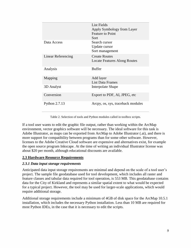
cumulative benefits to using the student-developed tool are shown below in Figure 5.
Table 5. Estimated cost savings over a nine week period with the geologic cross section tool (assuming full
operating capacity with 3 geologists and 5 student assistants). All values are in dollar amounts.
18
Table 6. Estimated expenditures over a nine week period using RockWorks proprietary software and estimated cost
for a contractor to develop the geologic cross section tool. All values are in dollar amounts.
Figure 5. Total cost savings vs. cost of alternative solutions. See row 7 from table 1 for cumulative total cost savings
input amounts and rows 2 and 4 from table 2 for RockWorks software and contractor cumulative costs input
amounts.
3.4 Benefit-Cost Analysis Conclusions
The development of a custom tool used for partially automating the creation of geologic cross
sections would provide numerous and significant benefits to GeoMapNW. Particularly Type 1
(efficiencies in current practices) and Type 2 (extended or additional benefits) benefit types can
be quantified and used as persuasive arguments for tool development in a cost benefit analysis.
Type 3 benefits (benefits related to unpredictable events) are also a significant factor and one that
should be presented in an argument in favor of developing the tool, although these are harder to
quantify and not applicable given the 9 week time scale that was considered in the cost-benefit
analysis presented here.
Due to the current semi-operational nature of GeoMapNW, the low cost of student tool
development, minimal training requirements for tool proficiency, and a minimal time investment
on behalf of GeoMapNW to commision the tool, the cost-saving benefits of this GIS project
clearly outweigh more expensive alternatives, such as the purchase of specialized software or
hiring a contractor to develop the tool. Of the three available scenarios, the construction of a

19
custom tool is the only one that presents cumulative benefits as opposed to cumulative costs. Due
to the nature of custom tool creation, this project will also deliver a product that will not require
extensive database reconfiguration to ensure compatibility.

20
4. DATA DEVELOPMENT
This project is focused on creating a geologic cross section tool to interact with existing data,
schemas, and data models. At project launch, Dr. Troost provided a well organized and extensive
geologic file geodatabase containing all data necessary for tool development. The objective of
the geologic cross section tool was to have the toolbox interact with other geologic file
geodatabases that may have a different file structure than GeoMapNW but will have a similar
database design based on join tables and feature classes joined through primary and foreign keys.
To begin development for the cross section tool design, Dr. Troost provided the authors with a
subset of the primary GeoMapNW database, complete with all feature classes, relationships,
tables, and rasters. This database was delivered to the City of Kirkland in 2018 in an effort to
assist them in revising Zoning Code 85 (Critical Areas: Geologically Hazardous Areas) for
public safety purposes in order to be in compliance with the Growth Management Act.
GeoMapNW’s database design was well thought out and organized, as its intended purpose is to
be used by a variety of public and private organizations. The database is used for site suitability
studies, seismic hazard assessment, groundwater infiltration studies, and planning hazard
mitigation strategies. The work GeoMapNW has done with the design of their database is
exceptionally detailed. The amount time and effort spent by GeoMapNW staff, project partners,
and students from the University of Washington to compile and integrate geotechnical and
geological engineering reports from over 100,000 borehole permit applications into the
GeoMapNW database represents an incredible investment of effort.
4.1 Data Acquisition
The ESRI file geodatabase was shared by Dr. Troost to us via DropBox and a Team Google
Drive we had set up for the project. Data acquisition was very straightforward, as the authors
simply download the data file and made a local copy on their personal computers for faster
processing. On the other hand, GeoMapNW is continuously adding more geologic data to their
database. Since GeoMapNW has opened by 2010 they had approximately 60,000 exploration
points from the Seattle area. Now they have integrated over 100,000 explorations into the
database.
In order for our tool to work with GeoMapNW’s database, the authors had conducted research to
possibly find past methods and solutions that would automate geologic cross sections. As said in
section 1.1.3, we found proprietary software that was too expensive and unrealistic, and we also
found VBA scripts that are no longer compatible with the current version of ArcGIS. We decided
our tool needed to be written with Python’s Arcpy module. Of the scripts we did find, our main
script heavily relies on Evan Thoms of the USGS geologic cross section tool created in 2005.
Thoms script is a beta version written with the Python Arcpy module. We streamlined Thoms’
script to work with GeoMapNW database.
4.2 Data Quality Issues
We did not encounter any data quality issues, due to receiving a functioning database that had all
the data requirements in order for our tool to work. We did not have to perform any post
processing of data. The unique ID field found in the feature classes and tables provided enough
detail in order to join attribute tables. There were no issues with GeoMapNW database apart
from possibly how data from the geotechnical reports they receive is processed and input. From
what we know, staff and students manually process the reports and integrate the data into their

21
database. This process is time consuming and can be prone to errors, although there are extensive
quality assurance (QA) procedures in place to mitigate human error. This process could be
automated by scraping pertinent information that will be included in the database.
Included in the data package we received from Dr. Troost, was a master ReadMEfile,
GeoMapNW Kirkland Geologic and Geological Hazards Maps and Products 2018 Master
ReadME file. In this file, we found explanations of data gaps that exist. Residential
neighborhoods, as an example is difficult to gather subsurface data from due to sound nuisance
that the drilling process would create. However, for our project this is not a concern. We did find
one issue with database design that would allow our tool function better. It would be helpful if
the tables were created as feature layers, as this would eliminate several steps in the scripting
process.
4.3 Future Data Preparation
The nature of our project involves the automation of data manipulation. We did not have to
manually alter the data provided, as the tool will perform these processes for the user. The user
will be responsible for providing minimal inputs and data, such as creating a cross section line
and specifying tool parameters including buffer distance from the cross section line for the
selection of explorations to be visualized. Our tool will perform three broad categories of tasks
involving the display of data. We have been assigned to 1) create an elevation profile in a cross
section view from an input line or selection of explorations, 2) create stick logs for each
exploration occurring along the input line or selected explorations, and 3) display additional
indicators, such as the groundwater depth and the density of the layers shown in the stick logs.
Each of these tasks requires additional data preparation as described below. Most preparation
will occur during the execution of our tool.
1) Elevation Profile Display
Input data must include a DEM and a transect line (or selection of explorations through which a
best fit transect will be generated). The transect line elevation values will be interpolated from
the DEM surface with the ‘Interpolate Shape’ tool. It will then be added to a new feature class
with an unknown spatial reference so that it can be displayed correctly in profile in a 2D setting.
2) Sticklog Display
Our tool requires turning geologic exploration locations and layer information into a 2D cross
sectional view of the layers selected near a transect line. In working to visualize a layer profile of
a borehole or similar exploration, it is beneficial to have a feature class or table that has a discrete
feature or row for each layer. Unfortunately, the data provided only offers the XY location of the
exploration in a point feature class. A layer table containing layer depth, composition, density,
and other Z information is joined to this feature class by a common exploration ID field
(EXPLOR_ID). In order to display each layer as a feature in ArcMap or ArcPro, we have
decided to create a line feature class, with the line length being proportional to the layer depth,
and the line location originating at the borehole location and extending downward. More details
of how this function works is in the results section 6.1.1.
22
3) Indicator display
Because indicator depth is known, displaying properties such as density and water table depth is
relatively simple. Interpolation of depth was used again, and linear referencing, route creation,
and/or cartographic buffers were be applied.
All data preparation should occur concurrent with tool use, and the data outputs will be minimal.
Feature classes created through intermediate processes are deleted or stored locally for reference.
4.4 Shared Group Challenges
GeoMapNW has done an exceedingly thorough job in data collection. Not once did we need to
find additional data not provided by the database, unless the originating geotechnical document
did not include values. An example of this is the exploration elevation field (EXPLOR_ELEV),
for which approximately half of the explorations have a value of 0 and an elevation source that is
null. This is because the height of the exploration was not recorded in the original geotechnical
document or supporting materials. Because the height was recorded as 0 and not as null, it is
difficult to tell which explorations truly originate at sea level and which have no actual elevation
record. To address this, our tool is able to interpolate heights for the exploration based on an area
DEM, although this is not always an accurate method and means that a cross section may display
stick logs for explorations that do and do not have initial elevations. Explorations without
elevations then appear to always begin on the DEM surface, even if they began in a local
depression or outcropping or terrain that was altered before or after the creation of the DEM.
Geologists using the tool will be made aware of this fact.
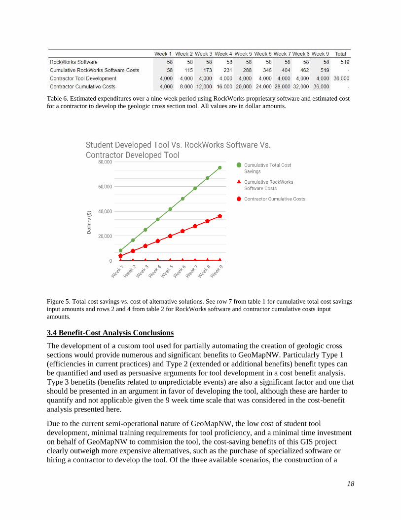
4.5 Database Schema Specifications
The following section will describe the database schema that we received from Dr. Troost. In
Table 7 is a list of rasters, tables, and feature classes that is required for the tool to work properly.
The full schema table GeoMapNW has compiled can be found in Appendix A, Table 10. In the
file geodatabase, we have a variety of raster layers, vector data (points, lines, and polygons) and
tables. Third-party databases that will be using the geologic cross section tool will need to have a
similar database structure for the tool to work correctly. For example, a unique ID field will need
to be made across all feature classes and tables in order to for the tool to function properly.
Field Name Source Spatial Object Type Description
Rasters
Kirk_Lidar GeoMapNW -
Kathy Troost Raster DEM
Feature Classes
Data_Points GeoMapNW -
Kathy Troost Point Surficial geology data
CrossSection User Line Create lines for cross sections
Tables

23
GROUNDWATER_WW GeoMapNW -
Kathy Troost Table
Groundwater data from exploration, and
well logs table
SUBSURF_LAYER GeoMapNW -
Kathy Troost Table Subsurface layer descriptions table
Tools
Sticklog&Groundwater&
Profile
Script created by
project group Script tool
Tool to create elevation profile,
sticklogs, and groundwater
Symbology Script created by
project group Script tool
Applies major material, density, and
groundwater symbology
Export2Graphic Script created by
project group Script tool Export to graphic output
Table 7. Database Schema Specifications. Required rasters, feature classes, tables, and tools that is required for the
geologic cross section tool to function using GeoMapNW database schema.
4.6 Description of Attribute Table Information
Attribute table information as described in Table 8 illustrates the work GeoMapNW has put into
compiling geologic records from boreholes, and other exploration records. For documentation
and metadata, GeoMapNW provided us with the GeoMapNW Kirkland Geologic and Geological
Hazards Maps and Products 2018 Master ReadME file. This file provided detailed information
about the attribute tables and the fields to be used in order for us to progress with our geologic
cross section tool development. The full attribute table information can be seen in Appendix A,
Table 11.
Field Name Description Data Type Length
EXPLOR_ID Exploration ID Long 10
EXPLOR_DEPTH Exploration Depth String 10
EXPLOELEV Exploration Elevation from report String 10
EXPLOELEVD Exploration Elevation from DEM Date 8
EXPLOR_ID Exploration ID Long 10
GROUNDWATER_DEPTH Depth to groundwater Float 8
EXPLOR_ID Exploration ID Long 10
LAYERTOPDE Layer Top Depth Float 8
LAYERBOTDE Layer Bottom Depth Float 8
DENSITYRAN Density Is Range? Short 5
MATDENSITY Material Density String 10

24
MATMAJOR Major Material Type String 10
Table 8. Attribute Table Specifications for DATA_POINT feature class and associated tables that are used in the
geologic cross section tool.
4.7 Content Metadata Descriptions
The table below is a data data dictionary containing descriptions of each dataset necessary for
tool operation. The full data directory can be seen in Appendix A, Table 12. Data quality
considers components of accuracy, resolution, consistency, and lineage across location, theme
and time, as described by Paradis and Beard (1994). Data lineage is described in detail in Section
1 of this document. Information for the dictionary came from the GeoMapNW Kirkland Geologic
and Geological Hazards Maps and Products 2018 Master ReadME file, data properties as
viewed in ArcCatalog, and metadata included with each data set. Because the tool was developed
for GeoMapNW, and GeoMapNW also created the data and desires a tool that will work with the
existing data and data structure, it can be assumed that in the context of GeoMapNW’s use of the
tool, the data is suitable. Although future improvements in accuracy, detail of attributes, or
coverage of exploration points across the region may be improved, the goal of the current project
is to create a tool for use with the existing data. Future improvements in data quality may,
however, lead to more accurate interpolations drawn from the data.
File Name Description Quality*
Kirk_Lidar Bare earth DEM 2016 Lidar; 3 feet resolution
Data_Points
Compilations of exposures and explorations from
subsurface investigations and observations at field
sites in City of Kirkland. This is the primary feature
class that will be used with the tool. Associated tables
(SUBSURF_LAYER, SUBSURF_COM,
BLOW_COUNT_WW, GROUNDWATER_WW)
should be used with this feature class for information
of subsurface layers and other details for each point
location.
Compiled by GeoMapNW 2010
and 2016-17 from outside
sources and validity/quality of
original data is not guaranteed.
Location accuracy is included as
an attribute field.
Kirk_Lakes Lakes in Kirkland polygon feature class. For general mapping purposes
only.
GROUNDWATER_WW
Groundwater data from multiple sources including
monitoring wells installed in subsurface explorations,
and water well logs. Includes depth to groundwater,
how depth was measured, and observation date. May
reflect seasonal groundwater occurrence. should be
joined to Data_Points layer using "exploration_id"
field.
Data compiled by GeoMapNW
2010 and 2016-2017
SUBSURF_LAYER Subsurface layer descriptions table; should be joined
to Data_Points layer using "exploration_id" field.
Data compiled by GeoMapNW
2010 and 2016-2017
Sticklog&Groundwater&Pr
ofile
Script to plot elevation profile, borehole stick logs and
groundwater in a cross-sectional view
This script heavily relies on
Evan Thoms of the USGS beta
version.

25
Symbology Script to apply symbology to major material, material
density, and groundwater Script created by project group
Export2Graphic Export current extent to graphic file Script created by project group
Table 9. Metadata descriptions for rasters, feature classes, tables and tools.

26
5. WORKFLOW IMPLEMENTATION
In order to provide a suitable deliverable to GeoMapNW at the culmination of the academic
quarter, a workflow processing plan was developed to guide both technical objectives and project
deadlines. This plan was primarily informed by the critical tool functions identified during
project scoping, and was used as a guide throughout the processes of tool development,
troubleshooting, user-testing, and delivery. The following section details the process involved in
the creation of the workflow processing plan and the resulting actual workflow used to create the
geologic cross section tool.
5.1 Determination of Deliverables
The format of the final cross section tool deliverable was discussed during a preliminary project
scoping meeting with Dr. Troost on 26 June, 2018. During that meeting it was explained that
GeoMapNW had developed a set of tools between 1999 and 2002 in Visual Basic for
Applications (VBA) for displaying down-hole geologic data in ESRI’s ArcView 3.x versions. An
example output from these tools is shown below in Figure 6. Due to the replacement of ArcView
with ArcGIS in 2000, these tools were quickly made obsolete. Additionally, prepackaged support
for the VBA programming language was discontinued with ArcGIS 10.x releases, requiring VBA
tools to be migrated to VB.NET or directly to compatible ArcGIS add-ins. This conversion
process was quickly decided to be both difficult and less useful than existing alternatives. It was
ultimately decided that the best practice would be to create a new Python-based tool by writing
Python script that could be executed from a script tool or tools housed in a shareable ArcGIS
toolbox. This script could be easily customized by users with basic Python familiarity to ensure
compatibility with new versions of ArcGIS and for eventual migration to ArcGIS Pro.
Figure 6. Output from a VBA tool developed for GeoMapNW displaying a 2D cross section including elevation profile and
geologic exploration layer composition.

27
Critical software capabilities were also identified by Dr. Troost during the scoping meeting. A
selection of outputs from the VBA tools were provided and used as a rough approximation of the
functionality that our tool should provide. At minimum, the tool should provide a 2D cross
section view of a surface profile and subsurface geologic layers drawn from an input cross
section line and a selection of geologic explorations from the GeoMapNW database, with
appropriate symbology applied to the layers so that material class and density are apparent.
Additionally, the tool should indicate groundwater depth when encountered and allow the user
customizable vertical and horizontal exaggeration and the ability to export the cross section to an
image file. These identified capabilities were distilled into a series of need-to-know questions
that could be addressed by our script and tool, including:
❏ What data points should be included in the cross section?
❏ What is the elevation profile along the cross section line?
❏ What is the location of each exploration and stick log relative to the cross section line?
❏ What is the major material of each subsurface layer?
❏ What is the density of each layer?
❏ What is the depth of each layer?
❏ What is the groundwater depth for each exploration?
❏ How will appropriate symbology be applied?
❏ How will the above be displayed visually in a graphic output?
Knowing the format of the final deliverable and focusing on key software capabilities identified
with these questions allowed for the creation of a workflow processing plan that included target
dates for the completion of scripts, a timeline for the creation of the final tool delivery, and plans
for user testing, implementation, and reporting.
5.2 Refining the Workflow Processing Plan
Following the identification of both deliverables and deadlines, further discussion of technical
limitations and considerations to the eventual user interface yielded a framework for the division
of software capabilities across multiple tools. It was decided that a main script would be written
for a tool to create an elevation profile, stick logs, and additional information requested by
GeoMapNW in a 2D cross section view. A second script would be written to apply symbology
and labels, and a third script would be written to export the current map view to an image file for
further processing. These tools would be packaged in an ArcToolbox integrated application (.tbx)
and constitute the primary deliverable to GeoMapNW. Secondary deliverables would include
tool help (both supporting documentation and in-line help from an HTML file or a compiled
.chm help file), symbology layers necessary for applying symbology to stick log material type,
density, and groundwater location, and the three scripts with developer commentary used for tool
creation. With deliverable requirements, capabilities, formats, and organization determined,
preliminary research was conducted to examine possible workflows.
Initial research regarding existing commercially-available cross section tools quickly confirmed
the problems that Dr. Troost mentioned regarding their suitability for her work and underscored
the need for the development of a custom tool. Most available software require licenses with
expensive pricing, and nearly all would require an alteration or additions to the GeoMapNW
exploration database schema. Further, a proprietary tool would not allow for data or tool sharing
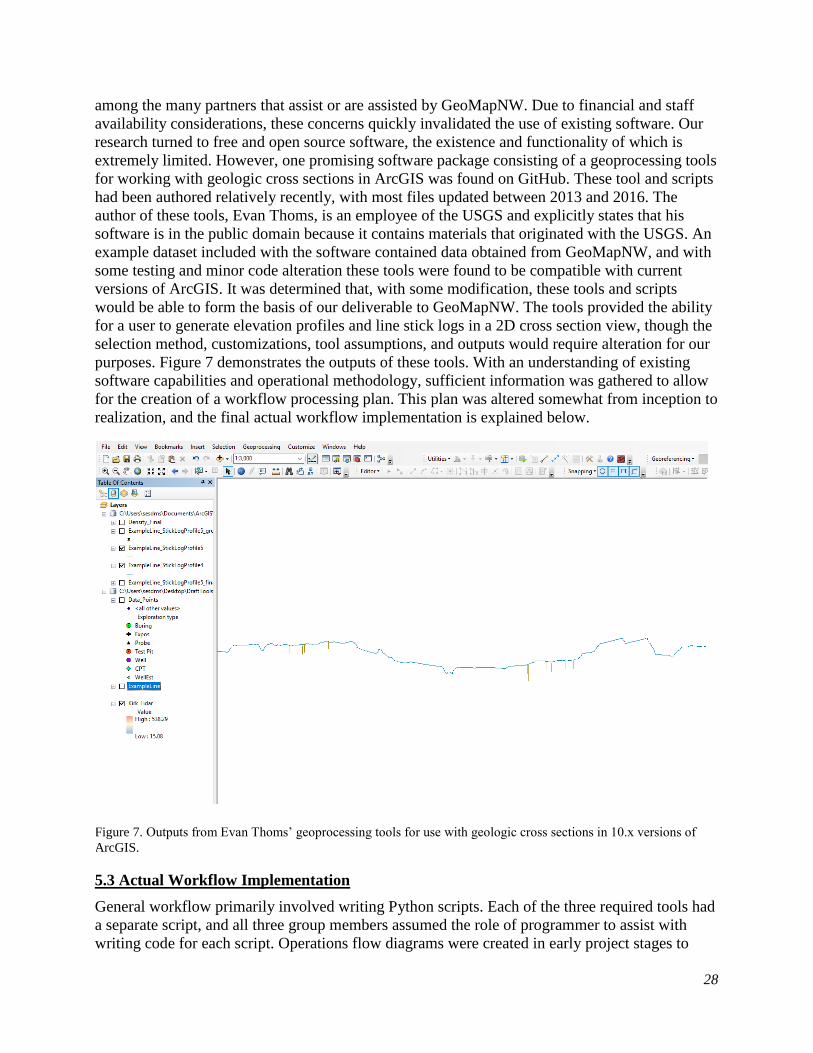
28
among the many partners that assist or are assisted by GeoMapNW. Due to financial and staff
availability considerations, these concerns quickly invalidated the use of existing software. Our
research turned to free and open source software, the existence and functionality of which is
extremely limited. However, one promising software package consisting of a geoprocessing tools
for working with geologic cross sections in ArcGIS was found on GitHub. These tool and scripts
had been authored relatively recently, with most files updated between 2013 and 2016. The
author of these tools, Evan Thoms, is an employee of the USGS and explicitly states that his
software is in the public domain because it contains materials that originated with the USGS. An
example dataset included with the software contained data obtained from GeoMapNW, and with
some testing and minor code alteration these tools were found to be compatible with current
versions of ArcGIS. It was determined that, with some modification, these tools and scripts
would be able to form the basis of our deliverable to GeoMapNW. The tools provided the ability
for a user to generate elevation profiles and line stick logs in a 2D cross section view, though the
selection method, customizations, tool assumptions, and outputs would require alteration for our
purposes. Figure 7 demonstrates the outputs of these tools. With an understanding of existing
software capabilities and operational methodology, sufficient information was gathered to allow
for the creation of a workflow processing plan. This plan was altered somewhat from inception to
realization, and the final actual workflow implementation is explained below.
5.3 Actual Workflow Implementation
General workflow primarily involved writing Python scripts. Each of the three required tools had
a separate script, and all three group members assumed the role of programmer to assist with
writing code for each script. Operations flow diagrams were created in early project stages to
Figure 7. Outputs from Evan Thoms’ geoprocessing tools for use with geologic cross sections in 10.x versions of
ArcGIS.

29
assist with conceptual understanding of script operation. These diagrams are presented in the
following sections to represent both how each script was written and how the script works by the
calling of specific functions and operations. Our scripting relied heavily on the Arcpy Python site
package, which benefits from being native to Python with access to numerous modules
developed for various GIS niche uses, code completion, and a variety of available functions and
classes. Operations flow diagrams are demonstrated below for each script written.
5.3.1 Stick Log and Elevation Profile Tool Operation Flow
The script to generate a 2D cross section view of stick logs, elevation profile, and groundwater
depth is the largest and most complex script, with 645 lines of code (including notation). This
script began as two separate scripts posted by Evan Thoms which were originally intended to
generate a surface profile from a cross section line and stick logs within a buffer distance from a
provided cross section line. These scripts were joined, common variables were identified, and
some extraneous functionality was removed. After a working script was obtained, modifications
to the original script were added to include the ability to:
❏ Select specific explorations to include in the output instead of relying on a buffer distance
from the line for finer control over the eventual 2D cross section output
❏ To allow for the user to specify the starting exploration elevation (the Y value from
which the exploration extends downward) as a field or to be interpolated from an
accompanying DEM
❏ To specify a horizontal exaggeration for the final output (in addition to included vertical
exaggeration)
❏ To create a point feature class representing groundwater location (depth), when
encountered in an exploration
❏ To buffer and order the stick log line outputs to better visually represent the outputs as
geologic layers appropriately located
The script is broken into several sections. It begins by importing necessary modules. Lines 24-
325 provide definitions for functions that are called for execution later in the script. Lines 332 to
395 define the parameters. The workspace is then set, and the main body of the script begins at
line 410. First, the ‘addAndCalc’ function is called, which adds a field (ORIG_FID) with an rkey
value to the cross section line that will undergo transformations that may overwrite the OID
value. The input line is then interpolated using the ‘arcpy.InterpolateShape_3d’ function, and a
zLines feature class is created. This is a near exact copy of the input line, but with an rkey field
and z value field added. M values are added to the zLines layer using the ‘arcpy.CreateRoutes_lr’
function, which creates accumulated measures by using the geometric length of the input features
and writing m values to a zmLines feature class. Measures are assigned according to the
coordinate priority specified by the user. Attributes from the original line input and the zmLines
layer are joined by using the ‘transferAtts’ function, which performs a join based on the
calculated rKey field and creates a new zmAtts feature class. Next, a new feature class,
zmProfiles, is created with an unknown spatial reference and the zmAtts feature class is
appended to it before calling the ‘plan2side’ function. This function updates the existing
geometry of the feature layer line and essentially changes the line from a 2D map (plane) view to
a 2D cross section (side) view by creating an array that transforms existing x and y values into z
and m values, where z values are obtained by interpolating the cross section line with the

30
arcpy.InterpolateShape_3d function and m values are measured distances from the beginning of
the cross section line to the exploration location (see Figure 8 for an illustration of this process).
Within this function, a drawing order is specified for the cross section line to determine where
the m values are drawn from and the horizontal and vertical exaggerations are applied as a
multiplier, if applicable. As the end result, this feature class is copied and provided in a feature
class as named by the user in a location specified by the user. This feature class is the cross
section line profile. Calculated rKey fields are deleted from the input line, and several
intermediate geoprocessing results are deleted. This process is shown in Figure 9.
Figure 8. A surface profile and stick log with an unknown spatial reference drawn using M and Z values obtained
from route measurement and elevation interpolation described in section 5.3.1.
After creating a surface elevation profile, the next code block creates stick logs from selected
explorations. First, selected explorations are interpolated to obtain a starting elevation if an
exploration elevation field is not specified or the field value is null using the
‘arcpy.InterpolateShape_3d function’. The resulting zBoreholes feature class contains
explorations that are located along the zmLines feature class from the previous surface profile
code block using the ‘arcpy.LocateFeaturesAlongRoutes_lr’ function. This function yields an
event table containing route IDs, route location data, and other information created during the
generation of z and m values for various feature classes in the creation of the surface profile
feature class. Exploration lines are then created by calling the boreholeLines function, which first
creates a new bhLines feature class and then opens a search cursor on the event table and an
insert cursor in bhLines. For each row in the event table, which contains a row for each
exploration that will be included in the bhLines feature class, the beginning y coordinates for the
points are set according to the borehole elevation or interpolated elevation multiplied by the
applicable vertical exaggeration. Ending y coordinates are calculated by applying the same
multiplier to the exploration depth. The x coordinates are calculated using the m values for the
location from the zmLine feature class, multiplied by the appropriate horizontal exaggeration.
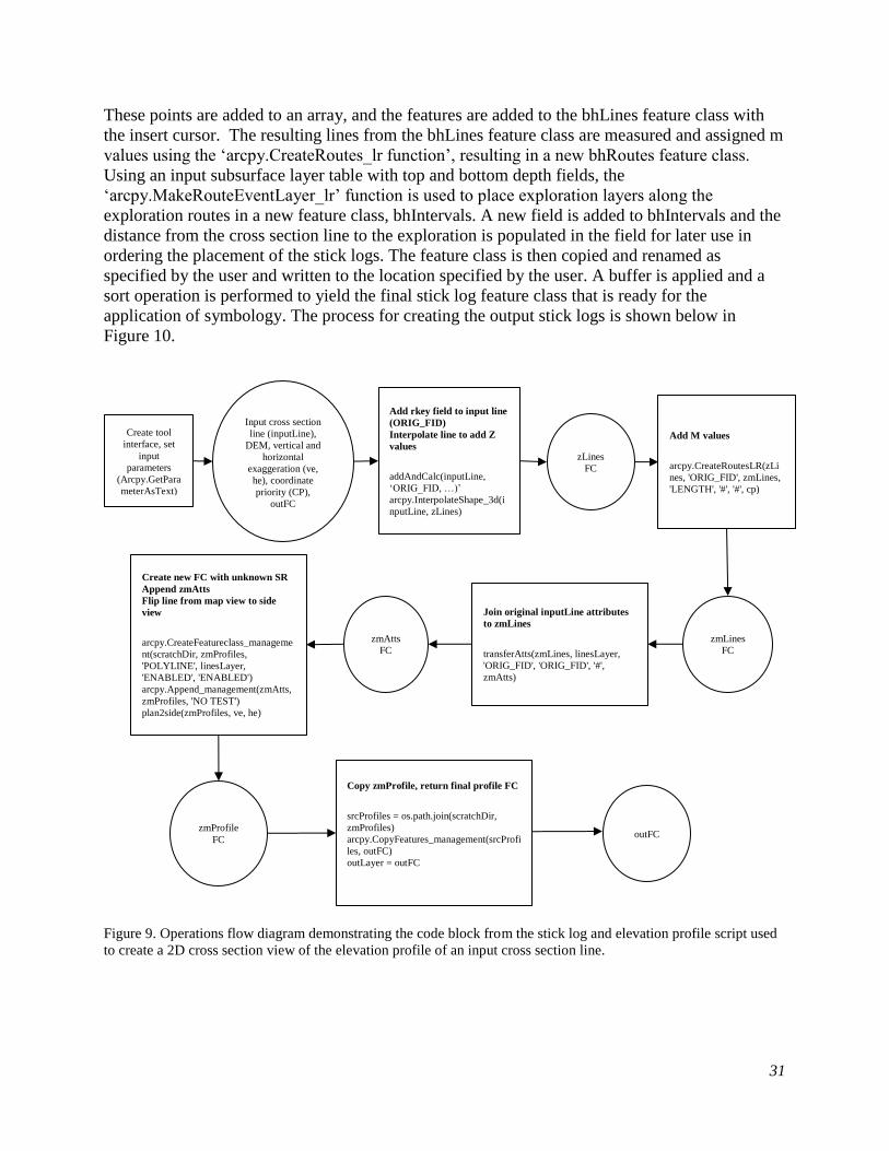
31
These points are added to an array, and the features are added to the bhLines feature class with
the insert cursor. The resulting lines from the bhLines feature class are measured and assigned m
values using the ‘arcpy.CreateRoutes_lr function’, resulting in a new bhRoutes feature class.
Using an input subsurface layer table with top and bottom depth fields, the
‘arcpy.MakeRouteEventLayer_lr’ function is used to place exploration layers along the
exploration routes in a new feature class, bhIntervals. A new field is added to bhIntervals and the
distance from the cross section line to the exploration is populated in the field for later use in
ordering the placement of the stick logs. The feature class is then copied and renamed as
specified by the user and written to the location specified by the user. A buffer is applied and a
sort operation is performed to yield the final stick log feature class that is ready for the
application of symbology. The process for creating the output stick logs is shown below in
Figure 10.
Figure 9. Operations flow diagram demonstrating the code block from the stick log and elevation profile script used
to create a 2D cross section view of the elevation profile of an input cross section line.
Create new FC with unknown SR Append zmAtts Flip line from map view to side
view arcpy.CreateFeatureclass_manageme
nt(scratchDir, zmProfiles,
'POLYLINE', linesLayer,
'ENABLED', 'ENABLED') arcpy.Append_management(zmAtts,
zmProfiles, 'NO TEST') plan2side(zmProfiles, ve, he)
Create tool
interface, set
input
parameters (Arcpy.GetPara
meterAsText)
Input cross section
line (inputLine),
DEM, vertical and
horizontal
exaggeration (ve,
he), coordinate
priority (CP),
outFC
Add rkey field to input line
(ORIG_FID) Interpolate line to add Z
values addAndCalc(inputLine,
‘ORIG_FID, …)’ arcpy.InterpolateShape_3d(i
nputLine, zLines)
zLines
FC
outFC
Add M values arcpy.CreateRoutesLR(zLi
nes, 'ORIG_FID', zmLines,
'LENGTH', '#', '#', cp)
zmLines
FC
Join original inputLine attributes
to zmLines transferAtts(zmLines, linesLayer,
'ORIG_FID', 'ORIG_FID', '#',
zmAtts)
zmAtts
FC
zmProfile
FC
Copy zmProfile, return final profile FC srcProfiles = os.path.join(scratchDir,
zmProfiles) arcpy.CopyFeatures_management(srcProfi
les, outFC) outLayer = outFC

32
Figure 10. Operations flow diagram demonstrating the code block from the stick log and elevation profile script used
to create a 2D cross section view of the stick logs from selected explorations.
After these operations are performed, lines 558-623 allow for the user to optionally create point
features that represent the groundwater location for each exploration, if encountered. This code
block first checks a boolean input; if true, the zBoreholes feature class is copied as a new feature
layer and joined to a table view of a provided groundwater table. An event table and gwaterLines
function is called that is a nearly identical copy of the borholeLines function, though the ending y
value is determined by the input groundwater depth field instead of the exploration depth field.
The resulting waterLines feature class is a line that begins at the exploration elevation and ends
at the groundwater depth. Geometry attributes are added to this line with the
‘arcpy.AddGeometryAttributes_management’ function, and the END_X field is updated using an
update cursor so that the eventual point will appear to the left of the stick log buffer instead of
inside the buffer polygon. An XY event layer is created using the
Create tool
interface, set
input parameters (Arcpy.GetParam
eterAsText)
Input selected
explorations,
exploration ID
field, exploration
elevation field,
exploration depth
field, subsurface
layer table,
Add DEM Z values for
explorations without an
exploration elevation field
value arcpy.InterpolateShape_3d
(dem, bhLayer, zBoreholes)
zBorehol
esFC
outFC
2
Add M values arcpy.LocateFeaturesAlong
Routes_lr(zBoreholes,
zmLines, 'ORIG_FID',
"5000 FEET", eventTable,
rProps, '#', 'DISTANCE')
Event
Table
Make exploration lines to be used
as routes boreholeLines() arcpy.CreateFeatureclass_managem
ent(scratchDir, bhLines,
'POLYLINE', zBoreholes,
'ENABLED', 'ENABLED') Insert Cursor Update Cursor Add Array
bhLine
s FC
Convert bhLines to event routes arcpy.CreateRoutes_lr(bhLines,
bhIdField, bhRoutes,
'ONE_FIELD', bhDepthField, '#',
'UPPER_LEFT') props = intBhIdFld + ' LINE ' +
intTopDepthFld + ' ' +
intBotDepthFld arcpy.MakeRouteEventLayer_lr(b
hRoutes, bhIdField,
intervalsTable, props, 'lyr', '#',
'ERROR_FIELD')
bhRoutes
FC
Copy bhRoutes, return final profile
FC Add dis2Xsec field, join event table
to outFC2 srcIntervals = os.path.join(scratchDir,
bhIntervals) arcpy.CopyFeatures_management(src
Intervals, outFC2) arcpy.JoinField_management(outFC2
, "EXPLOR_ID", eventTable,
"EXPLOR_ID") arcpy.CalculateField_management(o
utFC2, "Dis2XSec", "!Distance!",
"PYTHON_9.3", "")
Apply buffer to outFC2 Sort by dis2Xsec arcpy.Buffer_analysis(outFC2,
outBuff, buffSize, "FULL",
"FLAT", "NONE", "",
"PLANAR") arcpy.Sort_management(outBuf
f, sortBuff, [["Dis2XSec",
"ASCENDING"]])
‘outFC2 +
finalStick
s’ FC

33
‘arcpy.MakeXYEventLayer_management’ function, resulting in a final feature class with the
specified outname and ‘_groundwater’. This process is shown below in Figure 11.
Figure 11. Operations flow diagram demonstrating the code block from the stick log and elevation profile script used
to create a point feature class for the location of groundwater for selected explorations.
With all major tool outputs accounted for, the script proceeds to delete the many intermediate
outputs from geoprocessing results. Though this could be avoided by writing to the in-memory
workspace, certain intermediate outputs can be used for other applications and a user is able to
keep those which they deem useful by simply hashing out the delete functions for the feature
class they would like to keep in the final lines of code.
5.3.2 Symbology Tool Operation Flow
The symbology tool is powered by a relatively compact script, with 102 lines of code. This script
primarily applies symbology to map layers from pre-packaged layer files included in the final
zipped folder using the ‘arcpy.ApplySymbologyFromLayer_management’ function. However,
the task of symbolizing density concurrent with major material type did result in the need for
some geoprocessing operations, as it was decided that the best way for creating text-based
density labels was to apply a symbology layer with custom marker symbols, due to the fact that
Create tool
interface, set
input
parameters (Arcpy.GetPa
Input selected
explorations,
groundwater
boolean input,
groundwater
table
Copy zBoreholes FC as a feature
layer, Join groundwater table to new layer arcpy.MakeFeatureLayer_managemen
t (zBoreholes, waterView) arcpy.MakeTableView_management
(gwTable, gwView) arcpy.AddJoin_management
(waterView, bhIdField, gwView,
bhIdField2)
waterVie
w FC
finalOut
FC
Add M values arcpy.LocateFeaturesAlongRo
utes_lr(waterView, zmLines,
'ORIG_FID', "5000 FEET",
eventTable2, rProps, '#',
'DISTANCE')
Event
Table2
Make exploration lines to be used as
routes gwaterLines() arcpy.CreateFeatureclass_managemen
t(scratchDir, bhLines, 'POLYLINE',
waterView, 'ENABLED',
'ENABLED') Insert Cursor Update Cursor Add Array
waterLines
FC
Add geometry attributes to waterLines Remove null values Add a field, populate with updated END_X Create XY Event Layer arcpy.AddGeometryAttributes_management(waterLine
s, "LINE_START_MID_END") arcpy.SelectLayerByAttribute_management(waterLines
, "NEW_SELECTION", "START_X IS NULL OR
START_Y IS NULL") arcpy.DeleteFeatures_management(waterLines) arcpy.AddField_management(waterLines, 'newX',
"DOUBLE") Update Cursor arcpy.MakeXYEventLayer_management(waterLines,
"newX", "END_Y", tempOut, spatial_ref)
tempOut
FC
Create a new layer to properly project GW
location arcpy.CopyFeatures_management(tempOut,
finalOut)
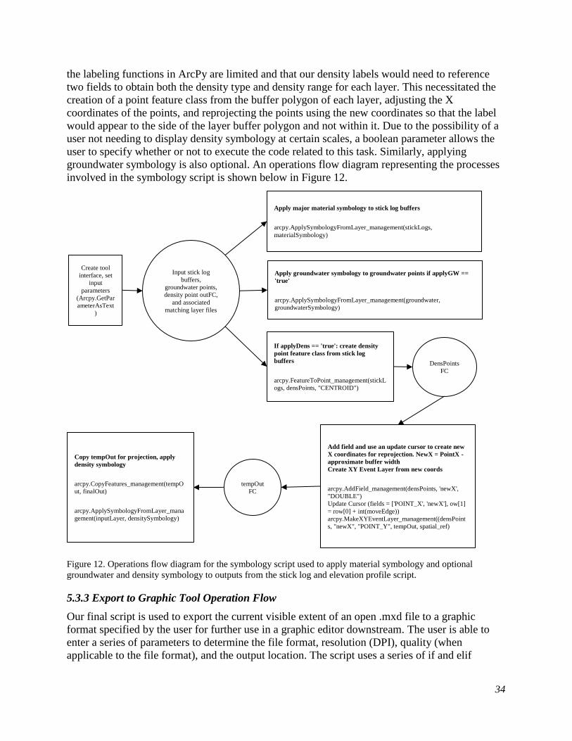
34
the labeling functions in ArcPy are limited and that our density labels would need to reference
two fields to obtain both the density type and density range for each layer. This necessitated the
creation of a point feature class from the buffer polygon of each layer, adjusting the X
coordinates of the points, and reprojecting the points using the new coordinates so that the label
would appear to the side of the layer buffer polygon and not within it. Due to the possibility of a
user not needing to display density symbology at certain scales, a boolean parameter allows the
user to specify whether or not to execute the code related to this task. Similarly, applying
groundwater symbology is also optional. An operations flow diagram representing the processes
involved in the symbology script is shown below in Figure 12.
Figure 12. Operations flow diagram for the symbology script used to apply material symbology and optional
groundwater and density symbology to outputs from the stick log and elevation profile script.
5.3.3 Export to Graphic Tool Operation Flow
Our final script is used to export the current visible extent of an open .mxd file to a graphic
format specified by the user for further use in a graphic editor downstream. The user is able to
enter a series of parameters to determine the file format, resolution (DPI), quality (when
applicable to the file format), and the output location. The script uses a series of if and elif
Create tool
interface, set
input
parameters (Arcpy.GetPar
ameterAsText
)
Input stick log
buffers,
groundwater points,
density point outFC,
and associated
matching layer files
Apply major material symbology to stick log buffers arcpy.ApplySymbologyFromLayer_management(stickLogs,
materialSymbology)
DensPoints
FC
Apply groundwater symbology to groundwater points if applyGW ==
'true' arcpy.ApplySymbologyFromLayer_management(groundwater,
groundwaterSymbology)
If applyDens == 'true': create density
point feature class from stick log
buffers arcpy.FeatureToPoint_management(stickL
ogs, densPoints, "CENTROID")
Add field and use an update cursor to create new
X coordinates for reprojection. NewX = PointX -
approximate buffer width Create XY Event Layer from new coords arcpy.AddField_management(densPoints, 'newX',
"DOUBLE") Update Cursor (fields = ['POINT_X', 'newX'], ow[1]
= row[0] + int(moveEdge)) arcpy.MakeXYEventLayer_management((densPoint
s, "newX", "POINT_Y", tempOut, spatial_ref)
tempOut
FC
Copy tempOut for projection, apply
density symbology arcpy.CopyFeatures_management(tempO
ut, finalOut) arcpy.ApplySymbologyFromLayer_mana
gement(inputLayer, densitySymbology)
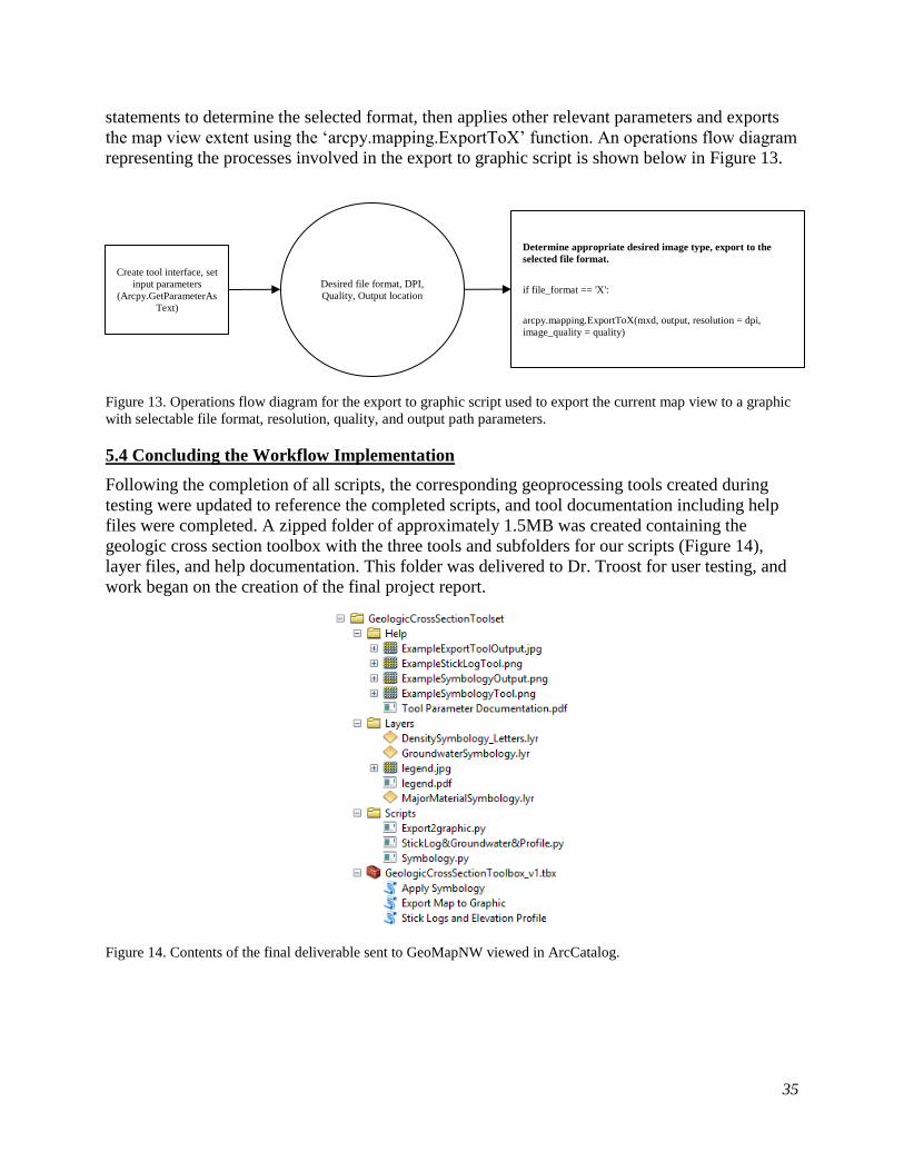
35
statements to determine the selected format, then applies other relevant parameters and exports
the map view extent using the ‘arcpy.mapping.ExportToX’ function. An operations flow diagram
representing the processes involved in the export to graphic script is shown below in Figure 13.
Figure 13. Operations flow diagram for the export to graphic script used to export the current map view to a graphic
with selectable file format, resolution, quality, and output path parameters.
5.4 Concluding the Workflow Implementation
Following the completion of all scripts, the corresponding geoprocessing tools created during
testing were updated to reference the completed scripts, and tool documentation including help
files were completed. A zipped folder of approximately 1.5MB was created containing the
geologic cross section toolbox with the three tools and subfolders for our scripts (Figure 14),
layer files, and help documentation. This folder was delivered to Dr. Troost for user testing, and
work began on the creation of the final project report.
Figure 14. Contents of the final deliverable sent to GeoMapNW viewed in ArcCatalog.
Create tool interface, set
input parameters (Arcpy.GetParameterAs
Text)
Desired file format, DPI,
Quality, Output location
Determine appropriate desired image type, export to the
selected file format. if file_format == 'X': arcpy.mapping.ExportToX(mxd, output, resolution = dpi,
image_quality = quality)

36
6. RESULTS
6.1 Tool Results
The primary results of concern are the geoprocessing outputs generated by the geologic cross
section tools. The following section presents results from our tools as they appear as outputs
from running the tools in ArcMap 10.5.1. Further testing in ArcMap 10.4.1 was conducted and
determined that outputs between these software versions were equivalent. The completed scripts
used by the cross section tools can be found in Appendix B.
6.1.1 Stick log and Surface Profile Tool Outputs
This tool successfully addressed several of the requested software capabilities identified during
project scoping. The user is able to manually select which geologic explorations will be included
in the tool output. The elevation profile of the cross section line is delivered from an input line,
and both horizontal and vertical exaggeration can be applied. The coordinate priority, or drawing
order, of this line can be specified by the user. The location of each exploration and associated
stick log relative to the cross section line is accurately depicted. The depth of each layer is
represented, and the location of encountered groundwater is plotted. The starting elevation for
selected exploration stick logs can be specified by using a field or by interpolation from an input
DEM. Finally, the user can specify the buffer width applied to the stick log lines that will be used
downstream for symbolizing material type for each subsurface layer. Due to the complexity of
the script, 17 required input parameters and 3 optional input parameters are necessary to provide
before running the tool. A typical selection process for explorations and cross section lines will
include manually selecting those elements from an open map document with necessary data
loaded, which is shown in Figure 15. The tool interface, with example parameters specified, is
shown below in Figure 16.
Figure 15. A map containing a selected cross section line, a DEM, and a selection of GeoMapNW geologic
explorations symbolized by exploration type (boring, test pit, CPT, etc). Once a selection has been made, the Stick
Log and Elevation Profile tool may be run.

37
Figure 16. The user interface for the Stick Log and Elevation Profile tool.
Running this tool results in three mandatory and one optional feature classes that are added by
the script to the data frame. This process is manually forced by the script in the event that the
geoprocessing settings of the user are not configured to automatically do so. These feature
classes include the elevation profile of the input cross section line (referenced as ‘outFC’ by the
script, and named by the user in the ‘Output Surface Profile’ parameter), output stick log route
lines (referenced as outFC2 by the script and named by the user in the ‘Output Stick Logs’
parameter), the sorted stick log buffers for selected explorations (named as ‘outFC2 +
‘_finalSticks), and an optional point feature class indicating groundwater depth (named as
‘outFC2 + ‘_groundWater). Running the tool with the example inputs above yielded the resulting
feature classes shown in Figure 17. An example of the tool functionality and flexibility is shown
in Figure 18, which demonstrates two results generated from the same selection of explorations
and profile line with different vertical and horizontal exaggeration and coordinate priorities
specified.

38
Figure 17. Geoprocessing results from the Stick Log and Elevation Profile tool. Feature classes include the surface
profile line, the sorted stick log buffer, stick log route lines (hidden behind the buffer), and the groundwater location
points (encountered in only two of the selected explorations).
Figure 18. Geoprocessing results from running the Stick Log and Elevation Profile tool with an identical cross
section line and selected explorations. The top result was run with 5x vertical exaggeration and 2x horizontal
exaggeration, with the line drawn from the northwest. The bottom result was run with 1x vertical and horizontal
exaggeration with the line drawn from the northeast.
Processing time takes approximately 0.5-4 minutes for tool execution, depending on available
RAM and the size of the cross section line and number of selected explorations. On a multi-core
machine with 16GB of RAM the tool was able to generate a stick log and elevation profile with
groundwater indicators for all explorations along a cross section line transecting the entire City
of Kirkland, WA (approximately 5 miles) in 4 minutes and 30 seconds (Figure 19). Average
selections of a dozen explorations or fewer take significantly less time.

39
Figure 19. Output from the Stick Log and Elevation Profile Tool with 6x vertical exaggeration for a transect line
crossing the entire City of Kirkland including stick logs for all GeoMapNW explorations within city limits. Stick
logs appearing significantly above or below the cross section line are located far enough away from the cross section
line that significant elevation changes may have occurred.
6.1.2 Apply Symbology Tool Outputs
The Apply Symbology tool successfully addressed several remaining requested software
capabilities identified during project scoping. After running the tool, the user is able to clearly
discern the major material type (sand, gravel, clay, etc) for each subsurface layer. A legend is
provided in the tool package in addition to being automatically generated in the map document
Table of Contents (Figure 20). Through the user interface the user is able to specify a stick log
feature class to apply symbology to, a major material type layer file from which symbology is
applied, a groundwater point feature class to apply symbology to, a groundwater depth layer file
from which symbology is applied, a material density point feature class location, a material
density layer file from which symbology is applied, the offset of the density labels (in map units),
and whether or not to display groundwater depth and/or material density for each layer when
information is available. An example of the tool UI with filled parameters is shown in Figure 21.
Processing time takes approximately 0.1-1 minute for tool execution, depending on available
RAM and the size of the cross section line and number of selected explorations. Choosing to
display density symbology is the longest operation to process since it involves running
geoprocessing tools and generating a new feature class.

40
Figure 20. A legend included in the geologic cross section toolbox providing a key for major material, density, and
groundwater symbols used by the Apply Symbology tool.
Figure 21. The user interface for the Apply Symbology Tool with example parameters provided.
Despite early challenges with displaying multiple levels of symbology simultaneously, the tool
output provides a clear representation of all three symbolized layers. Major material class type is
symbolized by the fill of the stick log buffer polygons. Density is displayed by applying symbol
levels to a point feature class that is generated and moved to the right edge of the layer buffer as
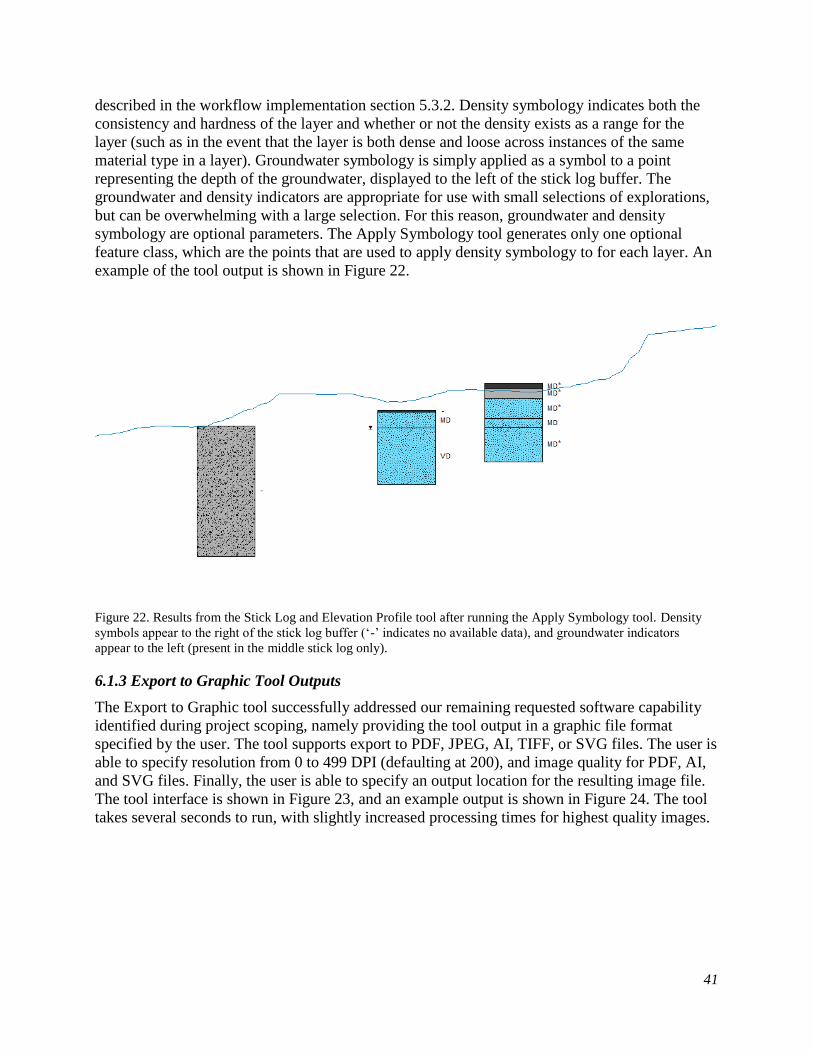
41
described in the workflow implementation section 5.3.2. Density symbology indicates both the
consistency and hardness of the layer and whether or not the density exists as a range for the
layer (such as in the event that the layer is both dense and loose across instances of the same
material type in a layer). Groundwater symbology is simply applied as a symbol to a point
representing the depth of the groundwater, displayed to the left of the stick log buffer. The
groundwater and density indicators are appropriate for use with small selections of explorations,
but can be overwhelming with a large selection. For this reason, groundwater and density
symbology are optional parameters. The Apply Symbology tool generates only one optional
feature class, which are the points that are used to apply density symbology to for each layer. An
example of the tool output is shown in Figure 22.
Figure 22. Results from the Stick Log and Elevation Profile tool after running the Apply Symbology tool. Density
symbols appear to the right of the stick log buffer (‘-’ indicates no available data), and groundwater indicators
appear to the left (present in the middle stick log only).
6.1.3 Export to Graphic Tool Outputs
The Export to Graphic tool successfully addressed our remaining requested software capability
identified during project scoping, namely providing the tool output in a graphic file format
specified by the user. The tool supports export to PDF, JPEG, AI, TIFF, or SVG files. The user is
able to specify resolution from 0 to 499 DPI (defaulting at 200), and image quality for PDF, AI,
and SVG files. Finally, the user is able to specify an output location for the resulting image file.
The tool interface is shown in Figure 23, and an example output is shown in Figure 24. The tool
takes several seconds to run, with slightly increased processing times for highest quality images.
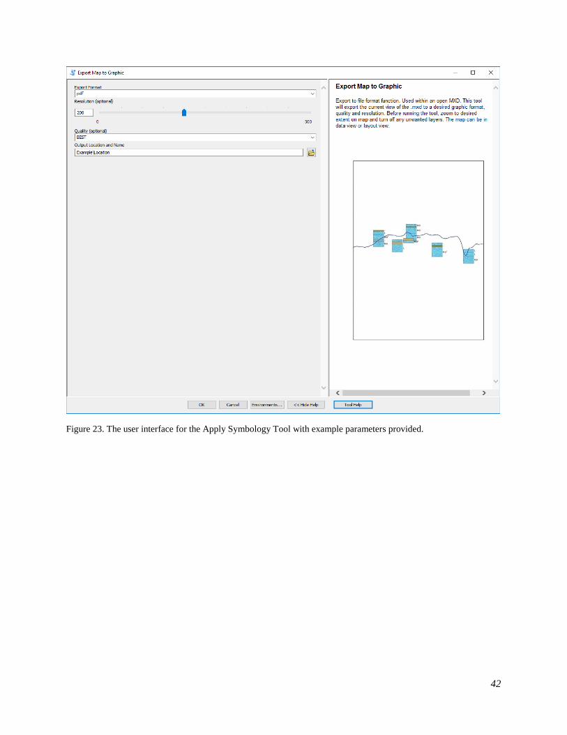
42
Figure 23. The user interface for the Apply Symbology Tool with example parameters provided.
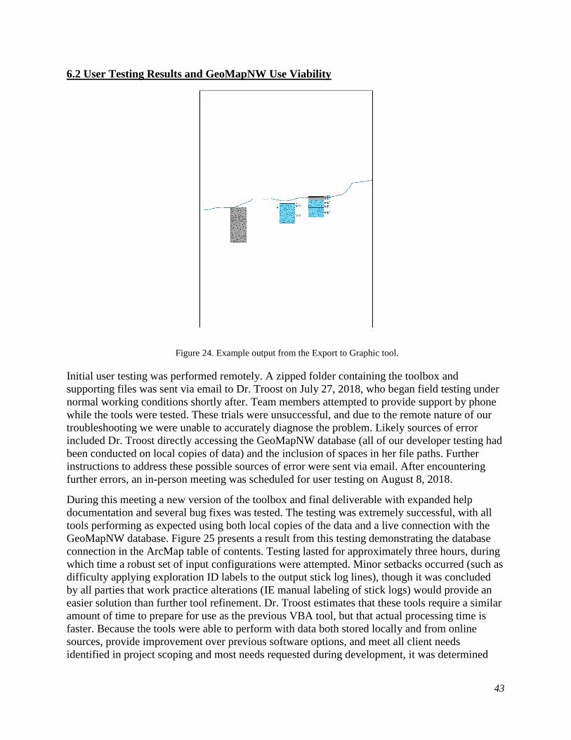
43
6.2 User Testing Results and GeoMapNW Use Viability
Initial user testing was performed remotely. A zipped folder containing the toolbox and
supporting files was sent via email to Dr. Troost on July 27, 2018, who began field testing under
normal working conditions shortly after. Team members attempted to provide support by phone
while the tools were tested. These trials were unsuccessful, and due to the remote nature of our
troubleshooting we were unable to accurately diagnose the problem. Likely sources of error
included Dr. Troost directly accessing the GeoMapNW database (all of our developer testing had
been conducted on local copies of data) and the inclusion of spaces in her file paths. Further
instructions to address these possible sources of error were sent via email. After encountering
further errors, an in-person meeting was scheduled for user testing on August 8, 2018.
During this meeting a new version of the toolbox and final deliverable with expanded help
documentation and several bug fixes was tested. The testing was extremely successful, with all
tools performing as expected using both local copies of the data and a live connection with the
GeoMapNW database. Figure 25 presents a result from this testing demonstrating the database
connection in the ArcMap table of contents. Testing lasted for approximately three hours, during
which time a robust set of input configurations were attempted. Minor setbacks occurred (such as
difficulty applying exploration ID labels to the output stick log lines), though it was concluded
by all parties that work practice alterations (IE manual labeling of stick logs) would provide an
easier solution than further tool refinement. Dr. Troost estimates that these tools require a similar
amount of time to prepare for use as the previous VBA tool, but that actual processing time is
faster. Because the tools were able to perform with data both stored locally and from online
sources, provide improvement over previous software options, and meet all client needs
identified in project scoping and most needs requested during development, it was determined
Figure 24. Example output from the Export to Graphic tool.
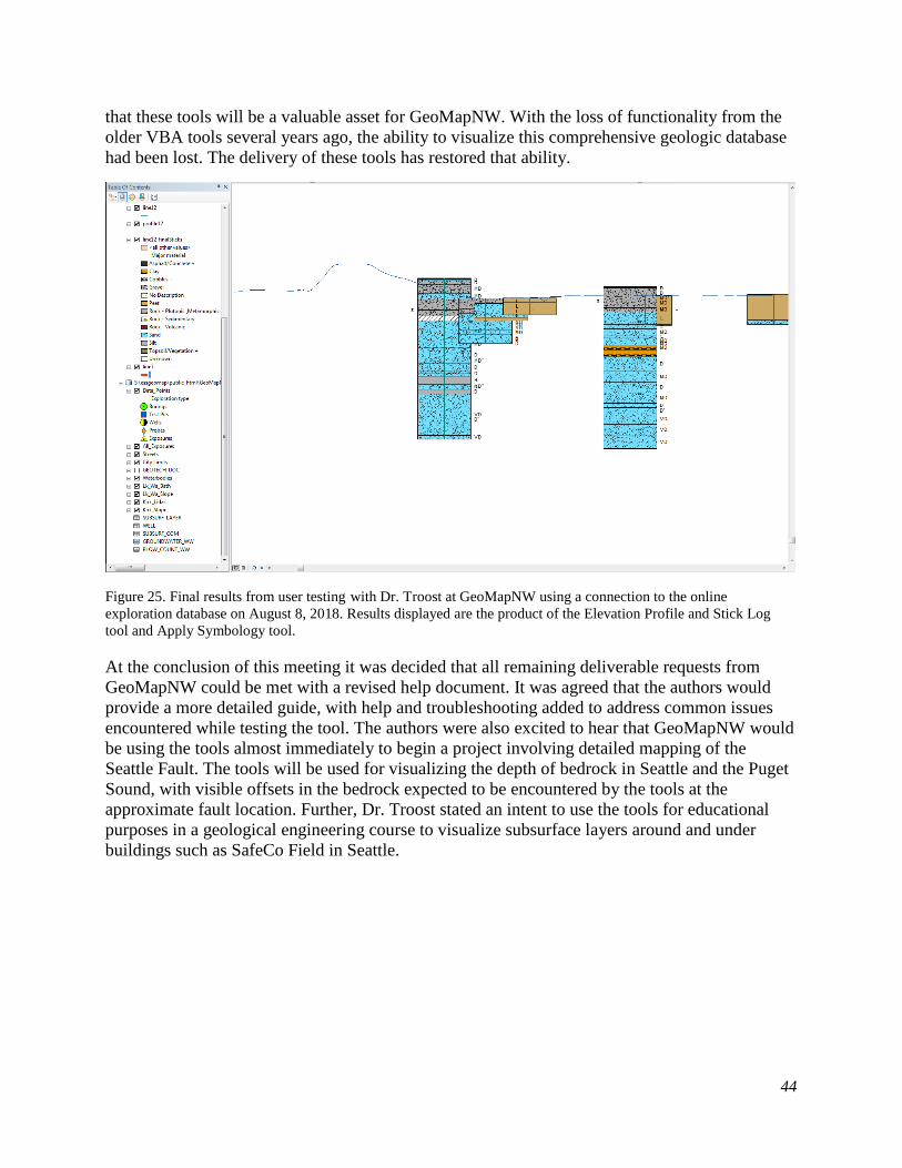
44
that these tools will be a valuable asset for GeoMapNW. With the loss of functionality from the
older VBA tools several years ago, the ability to visualize this comprehensive geologic database
had been lost. The delivery of these tools has restored that ability.
Figure 25. Final results from user testing with Dr. Troost at GeoMapNW using a connection to the online
exploration database on August 8, 2018. Results displayed are the product of the Elevation Profile and Stick Log
tool and Apply Symbology tool.
At the conclusion of this meeting it was decided that all remaining deliverable requests from
GeoMapNW could be met with a revised help document. It was agreed that the authors would
provide a more detailed guide, with help and troubleshooting added to address common issues
encountered while testing the tool. The authors were also excited to hear that GeoMapNW would
be using the tools almost immediately to begin a project involving detailed mapping of the
Seattle Fault. The tools will be used for visualizing the depth of bedrock in Seattle and the Puget
Sound, with visible offsets in the bedrock expected to be encountered by the tools at the
approximate fault location. Further, Dr. Troost stated an intent to use the tools for educational
purposes in a geological engineering course to visualize subsurface layers around and under
buildings such as SafeCo Field in Seattle.

45
7. CONCLUSIONS AND RECOMMENDATIONS
7.1 Conclusions Regarding Tool Suitability and Client Adoption
After providing and testing the final tool deliverable, it was determined by GeoMapNW that the
cross section tools would be put to use by the organization with near immediacy. Despite this
successful trial and adoption decision, it will likely be some time before the tools can be
sufficiently field tested to assess the true full suitability for client needs, due to low staffing.
Long-term cumulative benefits from the automation of creating cross section profiles from these
tools will only be realized after sustained use that may not occur in the immediate future.
However, smaller realized benefits will occur in the very near future with commencement of the
Seattle Fault location project, which will be made significantly easier with these tools. The
authors remain optimistic about initial tool testing results and are excited to see such immediate
adoption and use of the tools.
Similarly, it is likely that the tools will not be immediately shared with GeoMapNW clients or
partners until they have been deemed suitable and fully adopted for use by GeoMapNW. This lag
time before full deployment should hopefully not be complicated by tool compatibility between
partner organizations. The tool was intentionally developed for use with current versions of
ArcMap and using a programming language fully supported by ESRI. If modifications became
necessary (e.g. modifying the tool for use in ArcGIS Pro) these should be achievable by another
student group or by GeoMapNW staff with basic to intermediate programming skills.
7.2 Conclusions Regarding Tool Capabilities Relating to Need-To-Know Questions
One method for determining tool success is to assess how the tools are able to answer the need-
to-know questions developed in project scoping and presented in section 1.2.1. These questions
are revisited in the subsections below, with tool actualized capabilities related to the relevant
question.
7.2.1 What data points should be included in the cross section?
By using the included select tools and interfaces in ArcGIS, tool users are able to manually select
the explorations they would like to see presented as stick logs in the tool output. This affords the
user complete control over inclusions and exclusions, and provides the client with with the
method of selection they originally requested. Early versions of the tool relied on the selection
method built into the cross section toolbox from Evan Thoms, which selected all explorations
within a user-supplied buffer distance from the input cross section line. The refinement of the
selection process present in this tool presents significant utility for GeoMapNW and is a major
success for the tool.
7.2.2 What is the elevation profile along the cross section line?
This tool successfully delivers the elevation profile for an input cross section line. Further, this
elevation profile can be drawn starting from the northwest, northeast, southwest, or southeast
through a user-supplied coordinate priority assignment. Vertical and horizontal exaggeration can
also be supplied in integer intervals which will apply to both the surface profile and stick log
outputs. This functionality uses the methodology present in the scripts written by Evan Thoms,
with the exception of horizontal exaggeration, which was an addition by the student developers.
Despite being delivered as an output with undefined spatial reference, points within the array
representing the profile contain accurate Z values, in map units. These may be queried to provide
46
surface elevations at selected locations. With these capabilities, the tool successfully addresses
all client needs related to delivering an elevation profile from a cross section line.
7.2.3 What is the location of each exploration and stick log relative to the cross section line?
By using event data and linear referencing, explorations and their associated output stick logs are
able to be placed accurately along the elevation profile returned from the input cross section line.
Due to possible horizontal exaggeration of the line and undefined spatial reference of the tool
output, this is a relative location dependent on coordinate priority, cross section line
characteristics, and other user specifications. This method of determining location was provided
in scripts written by Evan Thoms. Student modifications to the scripts added the ability for stick
logs to be sorted by their perpendicular distance from the cross section line, which allows the
tool to display the relative distance from the cross section line to each stick log when stick logs
overlap. This provides rudimentary 3D capabilities to an otherwise 2D output. Aside from stick
log overlap priority placement, no means for determining the relative distance from the stick log
to the elevation profile exist. However, this need was not identified by the client during project
scoping. Current outputs satisfy all client requests and represent another successful technical
capability of the tool.
7.2.4 What is the major material of each subsurface layer?
Through application of a buffer to the output stick log lines generated by the tool, a rectangular
polygon of customizable size is added to the map view at the location of each subsurface layer.
By using the Apply Symbology tool, these polygons can be used to quickly differentiate between
the major material of each layer. An included legend with the final deliverable and a generated
table of contents legend in ArcMap provide a key for interpreting the symbology. This method
for representing major material types for each layer satisfies client requests, though it requires
running two tools: one to generate stick logs and one to apply symbology. This process could
have been streamlined into one tool, though by using a second tool for symbology application a
user is able to provide their own symbology layer file if desired and the overall complexity of the
stick log tool is reduced. This tool capability is another success and relies entirely on original
scripting provided by the student developers.
7.2.5 What is the density of each layer?
Density for each subsurface layer is applied again through the application of symbology. The
Apply Symbology tool creates points from the center of each stick log polygon which are shifted
to the polygon edge and labeled according to both density and whether or not the density ranges
throughout the layer. Several draft scripts experimented with applying density symbology as a
stick log polygon border, with thicker borders representing denser layers. Attempts were also
made to label density with a graphic line indicator similar to original outputs from the
GeoMapNW VB tool, though this method was also abandoned in favor of the more successful
method presented here. This tool capability again is derived from original student development
and represents a successful completion of client requests.
7.2.6 What is the depth of each layer?
Layer depths are generated by locating the points along the exploration route that correspond to
the layer top depth and layer bottom depth, which are field inputs provided by the user. The
location of these points are altered appropriately by the provided vertical exaggeration and used

47
to generate stick log line segments that begin at the layer top and extend down to the layer
bottom.
7.2.7 What is the groundwater depth for each exploration?
The groundwater depth for each exploration point can be optionally displayed as a marker
symbol located at the groundwater depth location along the side of each stick log where the data
is available. The groundwater points are created within the “Profile and Stick Logs” tool, and
symbology can be applied from within the “Symbology” tool. To create the markers, the script
follows similar steps to those used to create the stick log lines. Using linear referencing, lines are
placed along the cross section line, and the length (depth) of each line is determined by the
groundwater depth value, found in a joined table of groundwater attributes. Each line is
converted into a single point located at the end (bottom) of the line, and this point is then shifted
to be displayed at the edge of the stick log polygon.
7.2.8 How will appropriate symbology be applied?
Symbology is applied through a separate tool called “Symbology.” This tool applies a user-
provided symbology definition stored in a layer file to the tool outputs. The tool symbolizes each
subsurface layer by major material class, and also optionally displays the density of each layer
and the groundwater depth observed at each point. Symbology layer files for major material,
density, and groundwater are included in a folder within the packaged tool. As necessary, users
can use the Symbology tool to apply layer files other than those provided with the tool package,
or manually alter the symbologies.
7.2.9 How will the above be displayed visually in a graphic output?
The final symbolized tool outputs can be exported to a graphic file format using the “Export to
Graphic” tool included in the toolbox. This tool is designed to provide a simplified workflow for
the export process, with minimal parameters. The user first manually pans and zooms to the
extent of the map desired for export, or alternatively creates a layout view of the desired portion
of the map. Layers within the export extent that the user does not wish to be included in export
must be removed or turned off. Upon opening the Export to Graphic tool, the user selects the
desired export file format and sets parameters for resolution and quality, and then the current
map extent is exported. If further customization of export options are required than those
provided by the tool, the map can be manually exported using the built-in ArcMap export
function found in the File menu.
7.3 Recommendations for Further Development
This project achieved its goal of developing a set of tools that met the specifications requested in
the original project scope, and also included additional useful functions identified by the authors
and the project sponsor during the course of tool development. Nevertheless, opportunities to
enhance functionality, improve the presentation of outputs, and simplify the workflow for tool
operation have been identified. Some of these recommendations were identified during the tool
development process, but given the short time period for project completion the authors were
unable to include them in the final product. Others were identified as enhancements outside the
scope of the current project that could expand its capabilities if undertaken in the future.
Recommendations for further development are discussed below.

48
7.3.1 Output scale
Profile line, stick log, groundwater and density feature classes generated by the toolbox have no
spatial reference and are assigned an “unknown” coordinate system. With an unknown
coordinate system, the map units and hence the scale are unknown. A scale bar or some other
indicator of scale is typically considered a necessary element in any professional map. In this
particular case a scale would be useful to provide references such as the length of the cross
section, the depth of subsurface layers, and the changes in elevation across the profile. Assuming
that the data frame is assigned the same coordinate system as a relevant input features, the map
units will be set to this coordinate system. This means that with vertical and horizontal
exaggeration values set to “1,” adding a scale bar to the map would provide an accurate reference
scale. However, if the data frame is set to an unknown or other coordinate system, or if vertical
or horizontal exaggerations are a value other than one, a scale bar would be inaccurate. In this
case, a less traditional method for representing map scale would need to be developed. Adding
dynamic text displaying the total length of the cross section line, or providing a “reference” stick
log with static, labeled layer depths are two ideas for including some information on the output
relating to scale.
7.3.2 Profile line and stick log drawing direction
The “Start drawing from” parameter in the Stick Logs and Elevation Profile script allows users to
specify the “coordinate priority,” or the quadrant from which to start drawing. This parameter
identifies which end of the line is considered the “start” for the profile line and stick log display.
Knowing the starting direction is critical for accurately interpreting the results. If an output is
created and then shared, it might be falsely assumed that the drawing direction is from the west
because maps commonly display west on the left hand side. Displaying the drawing direction on
the output would be useful and would reduce errors resulting from misinterpretation of the line
direction. In its current configuration, the tool output does not provide a visual indication of the
chosen drawing direction, nor have the authors identified a simple way to manually add this
information. Creating a function within the tool that would add a drawing direction indicator to
the map would be a useful improvement.
7.3.3 Outputs with no spatial reference to separate data frame
Profile line and stick log outputs have no spatial reference, and thus appear on the map in an
arbitrary location, separate from the input cross section line and data points. It would be useful to
have the tool automatically add these outputs to a new data frame. This would enable adding
some additional mapping automation using the arcpy.mapping module (for example,
automatically panning and zooming to the extent of the outputs when the tool executes).
Additionally, a separate data frame would simplify the process of creating a map layout that
displays both the plane view cross section line and exploration points as well as the cross section
view profile line and stick log outputs.
7.3.4 Include template .mxd file to facilitate tool use
Related to the recommendations for a separate data frame for tool outputs discussed above, a
template .mxd file could be included with the packaged toolbox to facilitate tool use. This would
be especially helpful for users with limited GIS skills, and additionally would allow for
expanding use of the arcpy.mapping module within the script, because the creation of new
objects is not supported within the mapping module (for example, neither creating a new .mxd

49
nor adding a new data frame is a supported function). A template .mxd could contain multiple
data frames, and a default map layout including a legend and page size and orientation
properties. A template could also incorporate some of the other recommendations discussed in
this section, such as objects to hold scale and drawing direction indicators.
7.3.5 Automate labeling of the stick logs
One client request that we were unable to accommodate was the automation of stick log labeling.
Because the desired label positioning requires use of the Maplex labeling engine, and because
saving and sharing label properties is not well supported within current versions of ArcMap, we
were unable to automate label creation. Tool documentation includes instructions for manually
adding labels with the desired position and orientation, but ideally this would be included as an
automated tool feature. It is possible that as support for labeling functionality increases within
the ArcGIS platform, a labeling function could be added to the symbology script. Alternatively,
different methods for labeling automation could be explored, if manually labeling proves too
cumbersome.
7.3.6 Delete extraneous results and improve tool efficiency
Running the three tools with all optional outputs included currently results in a total of eight
outputs (6 feature classes, 1 table, and 1 graphic file). At least one of these outputs has been
identified as extraneous, however an unidentified bug in the script prevents the feature class from
being deleted automatically. It would be ideal to remove this extra data from the final results.
Additionally, as the client further assesses tool suitability, some of the other outputs may be
identified as unnecessary; the script could easily be modified to delete those outputs.
A related improvement would be to have the intermediate results stored in the in-memory
workspace, rather than written to the output location and then deleted. This would improve tool
performance and reduce the processing and storage requirements for the user. The process of
modifying the script to store intermediate results in-memory should be fairly simple.
7.3.7 Optional 3D output for use in ArcScene
The current tool produces results suitable for display in a 2D environment. Future development
could add functionality for converting these results into a format suitable for viewing in a 3D
environment, such as ArcScene. In addition to the more “realistic” view provided in a 3D
environment, having 3D results would be beneficial because the coordinate system could be
defined and results could be displayed in a spatially accurate location along with a
contextualizing basemap. This would be possible because within the 3D environment,
visualization of Z-values is an inherent capability. In a 2D environment it is not, and thus for the
outputs of this tool Z values are stored as X-coordinates within the features, essentially
“overwriting” a feature’s actual location.
7.3.8 Development for ArcGIS Pro
It is expected that ESRI will discontinue support for its ArcGIS Desktop products in 2024, by
which point Desktop users should be migrated to the ArcGIS Pro environment. In anticipation of
this event, it would be ideal to develop the toolbox for use in ArcGIS Pro. Creating a tool for use
with ArcGIS Pro would also provide additional benefits. Projects within the Pro environment are
packaged such that a multiple layout templates can be created for a single map. Also, 2D views
as well as a 3D views (“Scenes”) can be created within the same project. Other benefits may

50
exist or be added as the capabilities of Pro are extended by ESRI. For example, additional
support for the automation of feature labeling may be added to Pro but not to Desktop software.
Overall, the project can be considered successful. A set of ArcGIS custom tools was developed
that achieved all the primary capabilities identified in project scoping, within the necessary
timeline. Nevertheless, there still exist many opportunities for refining the tool and expanding its
functionality.

51
8. REFERENCES
Antenucci, John C. 1991. "Benefits and Costs." In Geographic Information Systems: A Guide to
the Technology, 65-82.
Booth, Derek B., Troost, Kathy G., Shimel, Scott A., O’Neal, Michael A., and Aaron P. Wisher.
2005. “New Geologic Mapping and Geologic Database for the Urbanized Puget Lowland,
Western Washington State, USA: U.S. Geological Survey Open-File Report 2005-1428.” In
Digital Mapping Techniques '05—Workshop Proceedings. USGS.
https://pubs.usgs.gov/of/2005/1428/booth/index.html
Carrell, Jennifer. 2014. “Tools and Techniques for 3D Geologic Mapping in ArcScene:
Boreholes, Cross Sections, and Block Diagrams.” USGS. Retrieved from
https://pubs.usgs.gov/of/2014/1167/pdf/ofr2014-1167_carrell-tools-and-techniques.pdf
Christensen, Arne. 2011. “What Lies Beneath? The Defunding of GeoMapNW.” The SunBreak,
November 22, 2011. http://thesunbreak.com/2011/11/22/what-lies-beneath-the-defunding-of-
geomapnw/
GeoMapNW. 2018. Kirkland Geologic and Geological Hazards Maps and Products 2018
Master ReadME file. Provided by Kathy G. Troost.
Huxhold, William. 1992. Multipurpose Land Information Systems Guidebook. Federal Geodetic
Coordinating Committee, Washington, D.C.
Paradis, J. and Beard, M. K. 1994. “Visualization of Spatial Data Quality for the Decision
Maker: A Data Quality Filter.” URISA Journal. 6(2): 25-34.
http://www.urisa.org/clientuploads/directory/Documents/Journal/vol6no2.pdf
Thoms, Evan. 2005. “U.S. Geological Survey Open-File Report 2005-1428: Creating and
Managing Digital Geologic Cross Sections within ArcGIS. U.S. Geological Survey Open-
File Report 2005-1428.” In Digital Mapping Techniques '05—Workshop Proceedings.
USGS. https://pubs.usgs.gov/of/2005/1428/thoms/index.html
Thoms, Evan. (n.d.). Python Cross-Section toolbox download from GitHub. Retrieved from
https://github.com/ethoms-usgs/Cross-Section
Troost, Kathy G., and Booth, Derek. B. 2005. “Cost of 1:12,000-Scale Geologic Map; $500,000:
Cost of 3D Data, Priceless.” GeoMapNW, University of Washington.
Troost, Kathy G., Brooks, Justin. L., Kohn, James. A., Teague, Kathryn E., Wisher, Aaron P.,
Thompson, Lauren. K., and Porter, Matthew J. 2017. “Kirkland Geology and Geological
Hazards Maps and Products.” GeoMapNW, Department of Earth and Space Sciences,
University of Washington, Seattle WA.

52
9. TECHNICAL APPENDICES
Appendix A: Data Design Tables
Table 10. Schema Specifications
Field Name Source Spatial Object
Type Description
Rasters
Kirk_Lidar GeoMapNW -
Kathy Troost Raster DEM
Kirk_Slope GeoMapNW -
Kathy Troost Raster DEM
Lk_Wa_Bath GeoMapNW -
Kathy Troost Raster Bathymetry
Lk_Wa_Slope GeoMapNW -
Kathy Troost Raster DEM
Feature Classes
All_Exposures GeoMapNW -
Kathy Troost Point Borehole data
Data_Points GeoMapNW -
Kathy Troost Point Surficial geology data
CityLimits GeoMapNW -
Kathy Troost PolyLine Kirkland study area
kirk_streets GeoMapNW -
Kathy Troost Line Kirkland streets
CrossSection Self Line Create lines for cross sections
GEOTECH_DOC GeoMapNW -
Kathy Troost Polygon Geotechnical reports from contractors
Kirk_Lakes GeoMapNW -
Kathy Troost Polygon Lakes in Kirkland
Tables
BLOW_COUNT_WW GeoMapNW -
Kathy Troost Table Subsurface geology ID table
GROUNDWATER_WW GeoMapNW -
Kathy Troost Table
Groundwater data from exploration, and
well logs table
SUBSURF_COM GeoMapNW -
Kathy Troost Table
Subsurface geology comments on
exploration logs table
SUBSURF_LAYER GeoMapNW -
Kathy Troost Table Subsurface layer descriptions table

53
WELL GeoMapNW -
Kathy Troost Table
Monitoring well data from exploration
logs table
Tools
Sticklog&Groundwater&Profile
Script created
by project
group Toolbox
Tool to create elevation profile, sticklogs,
and groundwater
Symbology
Script created
by project
group Toolbox
Applies major material, density, and
groundwater symbology
Export2Graphic
Script created
by project
group Toolbox Export to graphic output
Table 11. Attribute Table Specifications
Field Name Description Data Type Length
EXPOSID Exposure ID String 40
EXPOSNAME Exposure Name String 40
EXPOSTYPE Exposure Type String 40
EXPOSADD Exposure Address String 40
LOCATCONF Location Confidence String 40
EXPOSELEV Exposure Elevation Float 8
ELEVSOURCE Elevation Source String 40
DATUMNAME Datum Name String 40
OBSERVER Observer String 40
EXPOSDATE Exposure Date (yyyymmdd format) Date 8
EXPLOR_ID Exploration ID Long 10

54
DOCID Document ID Long 10
EXPLONAME Exploration Name String 50
EXPLOTYPE Exploration Type String 10
NORTHING Northing, State Plane North Float 8
EASTING Easting, State Plane North Float 8
LOCATCONF Location Confidence String 10
EXPLODEPTH Exploration Depth String 10
EXPLOELEV Exploration Elevation from report String 10
EXPLOELEVD Exploration Elevation from DEM Date 8
ELEVSOURCE Elevation Source String 10
DATUMNAME Datum Name String 10
AUTHORNAME Author Name Short 5
EXPLODATE Exploration Date (yyyymmdd format) Short 5
BORINGMETH Boring Method Date 8
CONTRACTOR Contractor Name String 10
ID Identification Double
MAINT_MAIN Maintenance Double
PERIMETER Kirkland Perimeter Double
ACRES Acres Double
HECTARES Hectares Double
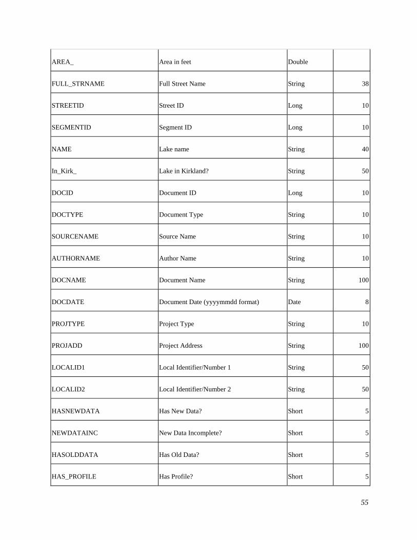
55
AREA_ Area in feet Double
FULL_STRNAME Full Street Name String 38
STREETID Street ID Long 10
SEGMENTID Segment ID Long 10
NAME Lake name String 40
In_Kirk_ Lake in Kirkland? String 50
DOCID Document ID Long 10
DOCTYPE Document Type String 10
SOURCENAME Source Name String 10
AUTHORNAME Author Name String 10
DOCNAME Document Name String 100
DOCDATE Document Date (yyyymmdd format) Date 8
PROJTYPE Project Type String 10
PROJADD Project Address String 100
LOCALID1 Local Identifier/Number 1 String 50
LOCALID2 Local Identifier/Number 2 String 50
HASNEWDATA Has New Data? Short 5
NEWDATAINC New Data Incomplete? Short 5
HASOLDDATA Has Old Data? Short 5
HAS_PROFILE Has Profile? Short 5

56
HAS_SLIDE Has Slide? Short 5
EXPLOR_ID Exploration ID Long 10
SUBSURF_LAYER_ID Subsurface Layer ID Long 10
BLOW_COUNTS_DEPTH Starting Depth of Sample Float 8
BLOW_COUNTS Sample Has Blow Counts Short 5
SPT Standard Penetration Test? Short 5
BLOW_COUNTS_1ST_6 Blows per 1st 6 inches Short 5
BLOW_COUNTS_2ND_6 Blows per 2nd 6 inches Short 5
BLOW_COUNTS_3RD_6 Blows per 3rd 6 inches Short 5
BLOW_COUNTS_4TH_6 Blows per 4th 6 inches Short 5
REFUSAL Blows before sample refused Short 5
PENETRATION Total Penetration at Refusal Short 5
SAMPLE_TYPE Sample Type String 10
SAMPLE_D_IN Sampler Diameter (inches) Float 8
ID_OD Inside or Outside diameter? Short 5
HAMMER_TYPE Hammer Type String 10
DROP_IN Hammer drop height Short 5
EXPLOR_ID Exploration ID Long 10
DOC_ID Document ID Long 10
EXPLOR_NAME Exploration Name String 50

57
GW_ENCOUNTERED Groundwater encountered? Short 5
GROUNDWATER_DEPTH Depth to groundwater Float 8
EXPLOR_DEPTH Depth of exploration Float 8
FLOWING Flowing water? Short 5
HEIGHT Height of water flow Float 8
DATE Observation date Date 8
DATA_SOURCE Data source type String 10
OBSERVATION_TYPE Groundwater observation type String 10
GROUNDWATER_DEPTHS Number of observations Short 5
GROUNDWATER_DEPTH_TYPE Which observation logged? String 10
COMID Comment ID Long 10
EXPLOR_ID Exploration ID Long 10
COMNUM Comment Number Short 5
COMDEPTH Comment Depth Float 8
COMDESC Comment Description String 400
LAYERID Layer ID Long 10
EXPLOR_ID Exploration ID Long 10
LAYERNUM Layer Number Short 5
LAYERTYPE Layer Type String 10
LAYERTOPDE Layer Top Depth Float 8

58
LAYERBOTDE Layer Bottom Depth Float 8
LAYERDESC Layer Description String 500
DENSITYRAN Density Is Range? Short 5
MATDENSITY Material Density String 10
MINORGRAV Material Is Gravelly? Short 5
MINORSAND Material Is Sandy? Short 5
MINORSILT Material Is Silty? Short 5
MINORCLAY Material Is Clayey? Short 5
MATMAJOR Major Material Type String 10
ORGANICS Material Has/Is Organic(s)? Short 5
DEBRIS Material Has Debris? Short 5
MATUSCS USCS on Log String 10
MATLOGUNIT Geologic Unit on Log String 50
WELLID Well ID Long 10
EXPLOR_ID Exploration ID Long 10
WELL_NAME Well Name String 50
WELL_DEPTH Well Depth Float 8
WELL_DIAME Well Diameter Float 8
SCREEN_TOP Depth of Screen (top) Float 8
SCREEN_BOT Depth of Screen (bottom) Float 8

59
SCREEN_GEO Geology at Screen String 10
NUM_READIN Number of Readings Short 5
LAST_READI Last Reading Date Date 8
LAST_REA_1 Last Reading Float 8
WELL_TESTI Well Testing Short 5
WATER_LEVE Water Level Type String 10
Table 12. Metadata Descriptions
File Name Description Quality
Kirk_Lidar Bare earth DEM for City of Kirkland 2016 Lidar; 3 feet resolution
Lk_Wa_Bath
Bathymetry data for the bottom of Lake
Washington, clipped 2000 feet from
shoreline
Data produced by NOAA, unknown date.
Cell size 28.25 feet.
Lk_Wa_Slope Slope DEM derived from Lk_Wa_Bath See Lk_Wa_Bath
All_Exposures
Compilation of exposures and their
attributes, from geologic field mapping
efforts in the City of Kirkland. Exposures
include roadcuts, landslide scarps,
riverbanks, excavations, etc.
Compiled by GeoMapNW 2010 and 2016-
17 from outside sources and
validity/quality of original data is not
guaranteed. Location accuracy is included
as an attribute field.
Data_Points
Compilations of exposures and
explorations from subsurface
investigations and observations at field
sites in City of Kirkland. Associated
table, SUBSURF_LAYER should be
used with this feature class for
information of subsurface layers for each
point location.
Compiled by GeoMapNW 2010 and 2016-
17 from outside sources and
validity/quality of original data is not
guaranteed. Location accuracy is included
as an attribute field.
Expo_Points Surficial geology data
GEOTECH_DOC
Spatial information (polygons) and
attributes about geotechnical reports;
spatial index of documents.
Data compiled by GeoMapNW 2010 and
2016-2017
BLOW_COUNT_WW
Blow count data compiled from borehole
logs. Includes depth of sample, blows per
6 inches, and details about samplers and
Data compiled by GeoMapNW 2010 and
2016-2017

60
hammers.
GROUNDWATER_WW
Groundwater data from multiple sources
including monitoring wells installed in
subsurface explorations, and water well
logs. Includes depth to groundwater, how
depth was measured, and observation
date. May reflect seasonal groundwater
occurance.
Data compiled by GeoMapNW 2010 and
2016-2017
SUBSURF_COM
Subsurface geology comments on
exploration logs table; should be joined
to Explorations layer using
"exploration_id" field.
Data compiled by GeoMapNW 2010 and
2016-2017
SUBSURF_LAYER Subsurface layer descriptions table Data compiled by GeoMapNW 2010 and
2016-2017
WELL
Monitoring well data from exploration
logs. Table can be joined to other layers
using "exploration_id" field.
Data compiled by GeoMapNW 2010 and
2016-2017
borehole Script to plot borehole stick logs in a
cross-sectional view
Beta version of script; limited
documentation.
sufaceprofile
Tool script to create one or more surface
profiles from an ArcMap line layer in a
cross sectional view shapefile. Requires a
line layer and a DEM in the same
coordinate system.
Can not check for schema lock; limited
documentation.
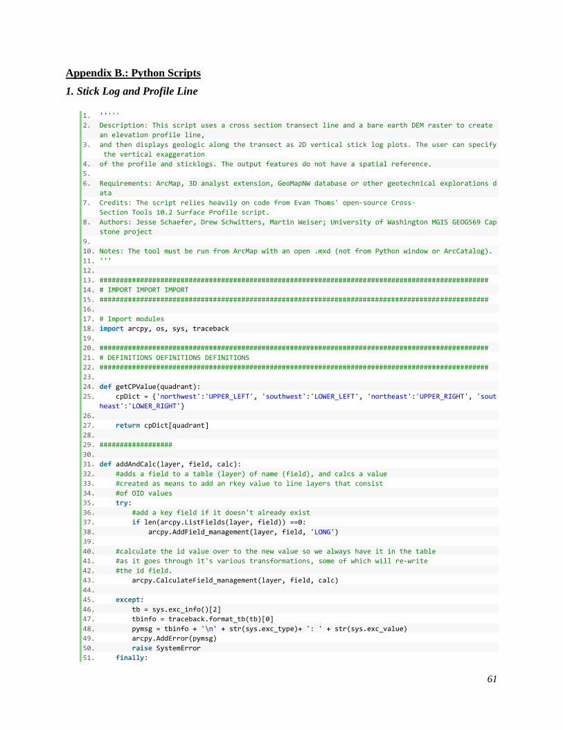
61
Appendix B.: Python Scripts
1. Stick Log and Profile Line
1. '''''
2. Description: This script uses a cross section transect line and a bare earth DEM raster to create
an elevation profile line,
3. and then displays geologic along the transect as 2D vertical stick log plots. The user can specify
the vertical exaggeration
4. of the profile and sticklogs. The output features do not have a spatial reference.
5.
6. Requirements: ArcMap, 3D analyst extension, GeoMapNW database or other geotechnical explorations d
ata
7. Credits: The script relies heavily on code from Evan Thoms' open-source Cross-
Section Tools 10.2 Surface Profile script.
8. Authors: Jesse Schaefer, Drew Schwitters, Martin Weiser; University of Washington MGIS GEOG569 Cap
stone project
9.
10. Notes: The tool must be run from ArcMap with an open .mxd (not from Python window or ArcCatalog).
11. '''
12.
13. ################################################################################################
14. # IMPORT IMPORT IMPORT
15. ################################################################################################
16.
17. # Import modules
18. import arcpy, os, sys, traceback
19.
20. ################################################################################################
21. # DEFINITIONS DEFINITIONS DEFINITIONS
22. ################################################################################################
23.
24. def getCPValue(quadrant):
25. cpDict = {'northwest':'UPPER_LEFT', 'southwest':'LOWER_LEFT', 'northeast':'UPPER_RIGHT', 'sout
heast':'LOWER_RIGHT'}
26.
27. return cpDict[quadrant]
28.
29. ##################
30.
31. def addAndCalc(layer, field, calc):
32. #adds a field to a table (layer) of name (field), and calcs a value
33. #created as means to add an rkey value to line layers that consist
34. #of OID values
35. try:
36. #add a key field if it doesn't already exist
37. if len(arcpy.ListFields(layer, field)) ==0:
38. arcpy.AddField_management(layer, field, 'LONG')
39.
40. #calculate the id value over to the new value so we always have it in the table
41. #as it goes through it's various transformations, some of which will re-write
42. #the id field.
43. arcpy.CalculateField_management(layer, field, calc)
44.
45. except:
46. tb = sys.exc_info()[2]
47. tbinfo = traceback.format_tb(tb)[0]
48. pymsg = tbinfo + '\n' + str(sys.exc_type)+ ': ' + str(sys.exc_value)
49. arcpy.AddError(pymsg)
50. raise SystemError
51. finally:

62
52. arcpy.RefreshCatalog
53.
54. ##################
55.
56. def addZ(ZptLayer):
57. #adds the z value to the table so that it is in the event table when we locate
58. #points along the line route
59. try:
60. arcpy.DeleteField_management(ZptLayers, 'DEM_Z')
61. except:
62. pass
63.
64. try:
65. arcpy.AddField_management(ZptLayer, 'DEM_Z', 'DOUBLE')
66. rows = arcpy.UpdateCursor(ZptLayer)
67. for row in rows:
68. # create the geometry object
69. feat = row.Shape
70. pnt = feat.getPart(0)
71. # set the value
72. row.setValue('DEM_Z', pnt.Z)
73. # update the row
74. rows.updateRow(row)
75.
76. except:
77. tb = sys.exc_info()[2]
78. tbinfo = traceback.format_tb(tb)[0]
79. pymsg = tbinfo + '\n' + str(sys.exc_type)+ ': ' + str(sys.exc_value)
80. arcpy.AddError(pymsg)
81. raise SystemError
82.
83.
84. ##################################
85.
86.
87. def transferAtts(inFC, joinTable, parentKey, childKey, fInfo, outName):
88. try:
89. #transfers attributes from a table to a fc: OIDs must match!
90. #get the attributes through a join which only works on a feature layer
91. lName = 'lay'
92. layer = arcpy.MakeFeatureLayer_management(inFC, lName)[0]
93.
94. #before the join, set the QualifiedFieldNames environment setting so that
95. #we don't see the source table name as a prefix in the field names
96. arcpy.env.qualifiedFieldNames = False
97.
98. #make the join based on key field
99. arcpy.AddJoin_management(lName, parentKey, joinTable, childKey)
100.
101. #copy features out to the output name
102. arcpy.CopyFeatures_management(lName, outName)
103.
104. except:
105. tb = sys.exc_info()[2]
106. tbinfo = traceback.format_tb(tb)[0]
107. pymsg = tbinfo + '\n' + str(sys.exc_type)+ ': ' + str(sys.exc_value)
108. arcpy.AddError(pymsg)
109.
110. ####################################
111.
112. def plan2side(ZMlines, ve, he):

63
113. #flip map view lines to cross section view without creating a copy
114. #this function updates the existing geometry
115. arcpy.AddMessage('Flipping ' + ZMlines + ' from map view to cross section view')
116. try:
117. rows = arcpy.UpdateCursor(ZMlines)
118. n = 0
119. for row in rows:
120. # Create the geometry object
121. feat = row.shape
122. new_Feat_Shape = arcpy.Array()
123. a = 0
124. while a < feat.partCount:
125. # Get each part of the geometry)
126. array = feat.getPart(a)
127. newarray = arcpy.Array()
128.
129. # otherwise get the first point in the array of points
130. pnt = array.next()
131.
132. while pnt:
133. pnt.X = float(pnt.M) * float(he)
134. pnt.Y = float(pnt.Z) * float(ve)
135.
136. #Add the modified point into the new array
137. newarray.add(pnt)
138. pnt = array.next()
139.
140. #Put the new array into the new feature shape
141. new_Feat_Shape.add(newarray)
142. a = a + 1
143.
144. #Update the row object's shape
145. row.shape = new_Feat_Shape
146.
147. #Update the feature's information in the workspace using the cursor
148. rows.updateRow(row)
149. except:
150. tb = sys.exc_info()[2]
151. tbinfo = traceback.format_tb(tb)[0]
152. pymsg = tbinfo + '\n' + str(sys.exc_type)+ ': ' + str(sys.exc_value)
153. arcpy.AddError(pymsg)
154. raise SystemError
155.
156. def boreholeLines():
157. #creates 2d cross section view sticklogs that show the depth of each borehole
158. try:
159. # create an empty output featureclass with the fields of the event table
160. arcpy.CreateFeatureclass_management(scratchDir, bhLines, 'POLYLINE', zBoreholes, 'ENABLED'
, 'ENABLED')
161.
162. # open search cursor on the event table
163. tRows = arcpy.SearchCursor(eventTable)
164.
165. # open insert cursor on the output layer
166. cur = arcpy.InsertCursor(bhLines)
167.
168. # create point and array objects
169. pnt1 = arcpy.CreateObject('Point')
170. pnt2 = arcpy.CreateObject('Point')
171. array = arcpy.CreateObject('Array')
172.

64
173. #get a list of fields in the template table that does not include OBJECTID or FID or SHAPE
174. #anything else? add it to xf! ("excluded fields")
175. xf = ('shape', 'objectid', 'fid', 'shape_length')
176. lf = arcpy.ListFields(zBoreholes)
177. names = []
178. for f in lf:
179. if not f.name.lower() in xf:
180. names.append(f.name)
181. #we also want the 'DISTANCE' value, calculated when the event table is built
182. #to be saved to this fc so it's needs to be in this list
183. names.append('distance')
184.
185. # enter while loop for each row in events table
186. for tRow in tRows:
187. # set the point's X and Y coordinates
188. # set Y depending on whether the user wants to use the elevation of the
189. # borehole from the DEM or from a value in the collar z field
190. try:
191. if bhElev == 0:
192. pnt1.Y = float(bhElev) * float(ve)
193. else:
194. pnt1.Y = float(tRow.getValue(zField)) * float(ve)
195. except:
196. arcpy.AddMessage('No collar elevation available for borehole ' + str(tRow.getValue
(bhIdField)))
197. arcpy.AddMessage('Using a value of 10000 for collar elevation')
198. pnt1.Y = 10000
199.
200. pnt1.X = tRow.RouteM * float(he)
201. pnt2.X = pnt1.X
202.
203. #if there is no value in bhDepthField, subtract 5000 from the top
204. #elevation as a way of flagging this point
205. try:
206. pnt2.Y = pnt1.Y - (float(tRow.getValue(bhDepthField) * float(ve)))
207. except:
208. arcpy.AddMessage(' No borehole depth available for borehole ' + str(tRow.getVal
ue(bhIdField)))
209. arcpy.AddMessage(' Using a value of 5000 for borehole depth.')
210. pnt2.Y = pnt1.Y - 5000
211.
212. # add points to array
213. array.add(pnt1)
214. array.add(pnt2)
215.
216. # set array to the new feature's shape
217. row = cur.newRow()
218. row.shape = array
219.
220. # copy over the other attributes
221. for name in names:
222. #try to write the value, but maybe the field can't be found or the value can't be
set
223. #for some reason. Don't want the whole thing to blow up
224. try:
225. row.setValue(name, tRow.getValue(name))
226. except:
227. #if it can't be written, forget about it
228. pass
229.
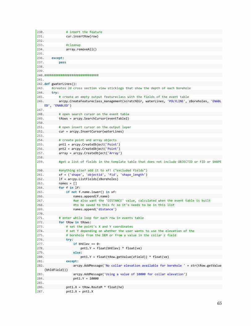
65
230. # insert the feature
231. cur.insertRow(row)
232.
233. #cleanup
234. array.removeAll()
235.
236. except:
237. pass
238.
239.
240. ##############################
241.
242. def gwaterLines():
243. #creates 2d cross section view sticklogs that show the depth of each borehole
244. try:
245. # create an empty output featureclass with the fields of the event table
246. arcpy.CreateFeatureclass_management(scratchDir, waterLines, 'POLYLINE', zBoreholes, 'ENABL
ED', 'ENABLED')
247.
248. # open search cursor on the event table
249. tRows = arcpy.SearchCursor(eventTable2)
250.
251. # open insert cursor on the output layer
252. cur = arcpy.InsertCursor(waterLines)
253.
254. # create point and array objects
255. pnt1 = arcpy.CreateObject('Point')
256. pnt2 = arcpy.CreateObject('Point')
257. array = arcpy.CreateObject('Array')
258.
259. #get a list of fields in the template table that does not include OBJECTID or FID or SHAPE
260. #anything else? add it to xf! ("excluded fields")
261. xf = ('shape', 'objectid', 'fid', 'shape_length')
262. lf = arcpy.ListFields(zBoreholes)
263. names = []
264. for f in lf:
265. if not f.name.lower() in xf:
266. names.append(f.name)
267. #we also want the 'DISTANCE' value, calculated when the event table is built
268. #to be saved to this fc so it's needs to be in this list
269. names.append('distance')
270.
271. # enter while loop for each row in events table
272. for tRow in tRows:
273. # set the point's X and Y coordinates
274. # set Y depending on whether the user wants to use the elevation of the
275. # borehole from the DEM or from a value in the collar z field
276. try:
277. if bhElev == 0:
278. pnt1.Y = float(bhElev) * float(ve)
279. else:
280. pnt1.Y = float(tRow.getValue(zField)) * float(ve)
281. except:
282. arcpy.AddMessage('No collar elevation available for borehole ' + str(tRow.getValue
(bhIdField)))
283. arcpy.AddMessage('Using a value of 10000 for collar elevation')
284. pnt1.Y = 10000
285.
286. pnt1.X = tRow.RouteM * float(he)
287. pnt2.X = pnt1.X

66
288.
289. #if there is no value in bhDepthField, subtract 5000 from the top
290. #elevation as a way of flagging this point
291. try:
292. if gwDepthField > 0:
293. pnt2.Y = pnt1.Y - (float(tRow.getValue(gwDepthField) * float(ve))) #changes bo
ttom Y value to groundwater depth times ve.
294. else:
295. pnt2.Y = float(bhElev) * float(ve)
296. except:
297. arcpy.AddMessage(' No groundwater depth available for borehole ' + str(tRow.get
Value(bhIdField)))
298. pnt2.Y = 0
299.
300. # add points to array
301. array.add(pnt1)
302. array.add(pnt2)
303.
304. # set array to the new feature's shape
305. row = cur.newRow()
306. row.shape = array
307.
308. # copy over the other attributes
309. for name in names:
310. #try to write the value, but maybe the field can't be found or the value can't be
set
311. #for some reason. Don't want the whole thing to blow up
312. try:
313. row.setValue(name, tRow.getValue(name))
314. except:
315. #if it can't be written, forget about it
316. pass
317.
318. # insert the feature
319. cur.insertRow(row)
320.
321. #cleanup
322. array.removeAll()
323.
324. except:
325. pass
326.
327. ################################################################################################
328. # PARMETERS PARAMETERS PARAMETERS
329. #################################################################################################
330.
331.
332. arcpy.env.overwriteOutput = True
333.
334. # Cross-section layer
335. linesLayer = arcpy.GetParameterAsText(0)
336.
337. # elevation raster layer
338. dem = arcpy.GetParameterAsText(1)
339.
340. #coordinate priority - corner from which the measuring will begin
341. cp = getCPValue(arcpy.GetParameterAsText(2))
342.
343. # vertical exaggeration (for both borehole lines and profile line)
344. ve = arcpy.GetParameterAsText(3)
345.
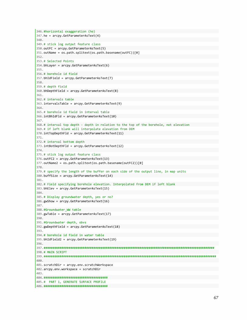
67
346. #horizontal exaggeration (he)
347. he = arcpy.GetParameterAsText(4)
348.
349. # stick log output feature class
350. outFC = arcpy.GetParameterAsText(5)
351. outName = os.path.splitext(os.path.basename(outFC))[0]
352.
353. # Selected Points
354. bhLayer = arcpy.GetParameterAsText(6)
355.
356. # borehole id field
357. bhIdField = arcpy.GetParameterAsText(7)
358.
359. # depth field
360. bhDepthField = arcpy.GetParameterAsText(8)
361.
362. # intervals table
363. intervalsTable = arcpy.GetParameterAsText(9)
364.
365. # borehole id field in interval table
366. intBhIdFld = arcpy.GetParameterAsText(10)
367.
368. # interval top depth - depth in relation to the top of the borehole, not elevation
369. # if left blank will interpolate elevation from DEM
370. intTopDepthFld = arcpy.GetParameterAsText(11)
371.
372. # interval bottom depth
373. intBotDepthFld = arcpy.GetParameterAsText(12)
374.
375. # stick log output feature class
376. outFC2 = arcpy.GetParameterAsText(13)
377. outName2 = os.path.splitext(os.path.basename(outFC2))[0]
378.
379. # specify the length of the buffer on each side of the output line, in map units
380. buffSize = arcpy.GetParameterAsText(14)
381.
382. # Field specifying borehole elevation. Interpolated from DEM if left blank
383. bhElev = arcpy.GetParameterAsText(15)
384.
385. # Display groundwater depth, yes or no?
386. gwShow = arcpy.GetParameterAsText(16)
387.
388. #Groundwater_WW table
389. gwTable = arcpy.GetParameterAsText(17)
390.
391. #Groundwater depth, obvs
392. gwDepthField = arcpy.GetParameterAsText(18)
393.
394. # borehole id field in water table
395. bhIdField2 = arcpy.GetParameterAsText(19)
396.
397. ################################################################################################
398. # MAIN SCRIPT
399. #################################################################################################
400.
401. scratchDir = arcpy.env.scratchWorkspace
402. arcpy.env.workspace = scratchDir
403.
404. ####################################
405. # PART 1, GENERATE SURFACE PROFILE
406. ####################################

68
407.
408. #add an rkey field to the table that consists of values from the OID
409.
410. desc = arcpy.Describe(linesLayer)
411. idField = desc.OIDFieldName
412. addAndCalc(linesLayer, 'ORIG_FID', '[' + idField + ']')
413.
414. #interpolate the lines
415. zLines = outName + '_z'
416. arcpy.AddMessage('Getting elevation values for features in ' + linesLayer)
417. arcpy.InterpolateShape_3d(dem, linesLayer, zLines)
418. arcpy.AddMessage(' ' + zLines + ' written to ' + arcpy.env.scratchWorkspace)
419.
420. #measure the lines
421. zmLines = outName + '_zm'
422. arcpy.AddMessage('Measuring the length of the line(s) in ' + zLines)
423. arcpy.CreateRoutes_lr(zLines, 'ORIG_FID', zmLines, 'LENGTH', '#', '#', cp)
424. arcpy.AddMessage(' ' + zmLines + ' written to ' + arcpy.env.scratchWorkspace)
425.
426. #hook the attributes back up
427. #transferAtts(inFC, joinTable, parentKey, childKey, fInfo, outName)
428. zmAtts = outName + '_zmAtts'
429. transferAtts(zmLines, linesLayer, 'ORIG_FID', 'ORIG_FID', '#', zmAtts)
430.
431. #make an empty container with an 'Unknown' SR
432. zmProfiles = outName + '_profiles'
433. arcpy.CreateFeatureclass_management(scratchDir, zmProfiles, 'POLYLINE', linesLayer, 'ENABLED', 'EN
ABLED')
434. arcpy.Append_management(zmAtts, zmProfiles, 'NO_TEST')
435. plan2side(zmProfiles, ve, he)
436.
437. #some cleanup
438. arcpy.DeleteField_management(zmProfiles, 'ORIG_FID')
439. arcpy.DeleteField_management(linesLayer, 'ORIG_FID')
440. arcpy.SelectLayerByAttribute_management(linesLayer, "CLEAR_SELECTION")
441. arcpy.Delete_management("lay")
442.
443. #copy the final fc from the scratch gdb to the output directory
444. srcProfiles = os.path.join(scratchDir, zmProfiles)
445. arcpy.CopyFeatures_management(srcProfiles, outFC)
446. outLayer = outFC
447.
448. ################################
449. #PART 2, GENERATE STICK LOGS
450. ################################
451.
452. #interpolate Z values for the boreholes
453. # first, select the borehole location points based on the buffer distance
454. #to minimize the processing time
455.
456. zBoreholes = outName2 + '_zBoreholes'
457. arcpy.InterpolateShape_3d(dem, bhLayer, zBoreholes)
458.
459. #add DEM Z values to zBoreholes attribute table
460. #might already be there so we'll try to add it
461. try:
462. arcpy.AddField_management(zBoreholes, 'zDEM', 'FLOAT')
463. except:
464. pass
465. #and calc in the geometry x
466. try:

69
467. arcpy.CalculateField_management(zBoreholes, 'zDEM', '!SHAPE.FIRSTPOINT.Z!', 'PYTHON_9.3')
468. except:
469. #if the elevation cannot be determined for some reason, calc 0
470. arcpy.CalculateField_management(zBoreholes, 'zDEM', 0, 'PYTHON_9.3')
471.
472. #'DEM_Z' becomes the collar elevation field
473. zField = 'zDEM'
474.
475. # locate boreholes points along the cross-section
476. eventTable = outName2 + '_bhEvents'
477. rProps = 'rkey POINT RouteM'
478. arcpy.AddMessage('Locating ' + zBoreholes + ' on ' + zmLines)
479. arcpy.LocateFeaturesAlongRoutes_lr(zBoreholes, zmLines, 'ORIG_FID', "5000 FEET", eventTable, rProp
s, '#', 'DISTANCE') #change the distance here if you want to include stick logs farther than 5000
map units from the cross section line
480. arcpy.AddMessage(' ' + eventTable + ' written to ' + arcpy.env.scratchWorkspace)
481.
482. #remove duplicate records that result from what appears to be
483. #an unresolved bug in the Locate Features Along Routes tool
484. #some points will get more than one record in the event table
485. #and slightly different, sub-mapunit, mValues
486. arcpy.DeleteIdentical_management(eventTable, bhIdField)
487.
488. # make the borehole lines to be used as routes
489. bhLines = outName2 + '_bhLines'
490. arcpy.AddMessage('Building lines in cross-section view from ' + eventTable)
491. boreholeLines()
492. arcpy.AddMessage(' ' + bhLines + ' written to ' + arcpy.env.scratchWorkspace)
493.
494. bhRoutes = outName2 + '_bhRoutes'
495. arcpy.AddMessage("Measuring the length of borehole lines in " + bhLines)
496. arcpy.CreateRoutes_lr(bhLines, bhIdField, bhRoutes, 'ONE_FIELD', bhDepthField, '#', 'UPPER_LEFT')
497. arcpy.AddMessage(' ' + bhRoutes + ' written to ' + arcpy.env.scratchWorkspace)
498.
499. #place borehole intervals (line events) on borehole routes
500. props = intBhIdFld + ' LINE ' + intTopDepthFld + ' ' + intBotDepthFld
501. arcpy.AddMessage("Placing borehole intervals on routes in " + bhRoutes)
502. arcpy.MakeRouteEventLayer_lr(bhRoutes, bhIdField, intervalsTable, props, 'lyr', '#', 'ERROR_FIELD'
)
503.
504. #extract only valid route events from this in-memory layer
505. arcpy.AddMessage('Filtering interval records with location errors.')
506. bhIntervals = outName2 + '_intervals'
507. arcpy.Select_analysis('lyr', bhIntervals, "\"LOC_ERROR\" <> 'ROUTE NOT FOUND'")
508. arcpy.AddMessage(' ' + bhIntervals + ' written to ' + arcpy.env.scratchWorkspace)
509.
510. # Create a field to represent the perpendicular distance from the cross section to the exploration
. This will be populated later.
511. arcpy.AddField_management(bhIntervals, 'Dis2XSec', 'DOUBLE')
512. layer2 = arcpy.MakeFeatureLayer_management(bhIntervals, 'lyr2')
513. arcpy.env.qualifiedFieldNames = False
514.
515. # Create the final output feature class
516.
517. srcIntervals = os.path.join(scratchDir, bhIntervals)
518. arcpy.CopyFeatures_management(srcIntervals, outFC2)
519. arcpy.AddMessage(' ' + bhIntervals + ' copied to ' + outFC2)
520. outLayer = outFC2
521.

70
522. # Join the out borehole feature class with the eventTable in order to pass over the 'DISTANCE' fie
ld
523. # which is the distance the sticklog is away from the cross-section line
524.
525. arcpy.JoinField_management(outFC2, "EXPLOR_ID", eventTable, "EXPLOR_ID")
526. arcpy.CalculateField_management(outFC2, "Dis2XSec", "!Distance!", "PYTHON_9.3", "")
527.
528. # Some cleanup
529. arcpy.DeleteField_management(arcpy.GetParameterAsText(0), 'ORIG_FID')
530.
531.
532. ################################################################################################
533. # PART 3 Prepare to apply symbology, display lines as layers
534. ################################################################################################
535.
536. # Apply a buffer to the stick logs generated to better visualize the layers
537.
538. outBuff = outFC2 + '_Buffer'
539. arcpy.Buffer_analysis(outFC2, outBuff, buffSize, "FULL", "FLAT", "NONE", "", "PLANAR")
540.
541. # Sort the buffer by the dis2Xsec field to simulate 3D placement (boreholes closer to the viewer w
ill appear ahead of others)
542.
543. sortBuff = outName2 + '_finalSticks'
544. arcpy.Sort_management(outBuff, sortBuff, [["Dis2XSec", "ASCENDING"]])
545.
546. # Add the buffer to the dataframe, if not done automatically
547.
548. mxd = arcpy.mapping.MapDocument("CURRENT")
549. dataFrame = arcpy.mapping.ListDataFrames(mxd, "*")[0]
550. addlayer = arcpy.mapping.Layer(sortBuff)
551. arcpy.mapping.AddLayer(dataFrame, addlayer, "TOP")
552.
553.
554. #################################################################################################
555. # PART 4 Add Groundwater Depth Indicators
556. #################################################################################################
557.
558. if gwShow == 'true':
559. waterView = outName2 + '_waterView'
560. arcpy.MakeFeatureLayer_management (zBoreholes, waterView)
561. gwView = outName2 + '_gwTableView'
562. arcpy.MakeTableView_management (gwTable, gwView)
563. arcpy.AddJoin_management (waterView, bhIdField, gwView, bhIdField2)
564.
565. eventTable2 = outName2 + '_bhEvents2'
566. rProps = 'rkey POINT RouteM'
567. arcpy.AddMessage('Locating ' + zBoreholes + ' on ' + zmLines)
568. arcpy.LocateFeaturesAlongRoutes_lr(waterView, zmLines, 'ORIG_FID', "5000 FEET", eventTable2, r
Props, '#', 'DISTANCE')
569. arcpy.AddMessage(' ' + eventTable + ' written to ' + arcpy.env.scratchWorkspace)
570.
571. waterLines = outName2 + '_waterLines'
572. gwaterLines()
573.
574. # Add XY data to the waterLines so that points can be made at the end representing groundwater
depth, if present
575. arcpy.AddGeometryAttributes_management(waterLines, "LINE_START_MID_END")
576.
577. # Add the waterLines to the map
578. mxd = arcpy.mapping.MapDocument("CURRENT")
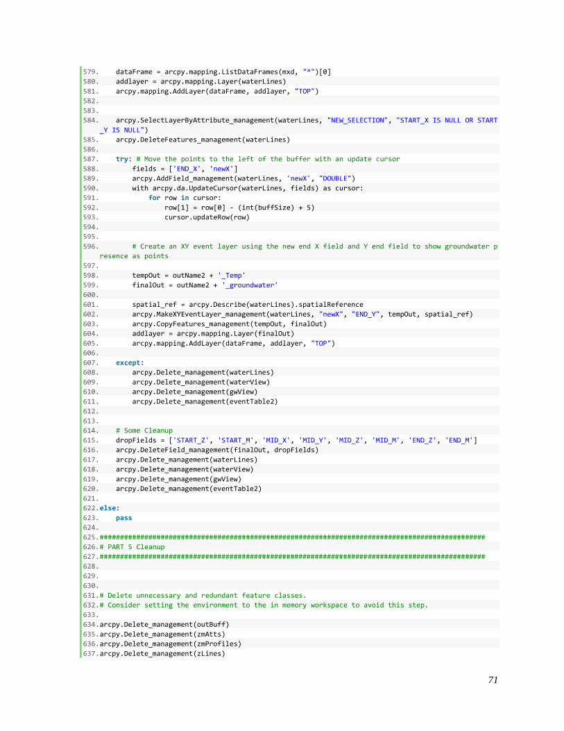
71
579. dataFrame = arcpy.mapping.ListDataFrames(mxd, "*")[0]
580. addlayer = arcpy.mapping.Layer(waterLines)
581. arcpy.mapping.AddLayer(dataFrame, addlayer, "TOP")
582.
583.
584. arcpy.SelectLayerByAttribute_management(waterLines, "NEW_SELECTION", "START_X IS NULL OR START
_Y IS NULL")
585. arcpy.DeleteFeatures_management(waterLines)
586.
587. try: # Move the points to the left of the buffer with an update cursor
588. fields = ['END_X', 'newX']
589. arcpy.AddField_management(waterLines, 'newX', "DOUBLE")
590. with arcpy.da.UpdateCursor(waterLines, fields) as cursor:
591. for row in cursor:
592. row[1] = row[0] - (int(buffSize) + 5)
593. cursor.updateRow(row)
594.
595.
596. # Create an XY event layer using the new end X field and Y end field to show groundwater p
resence as points
597.
598. tempOut = outName2 + '_Temp'
599. finalOut = outName2 + '_groundwater'
600.
601. spatial_ref = arcpy.Describe(waterLines).spatialReference
602. arcpy.MakeXYEventLayer_management(waterLines, "newX", "END_Y", tempOut, spatial_ref)
603. arcpy.CopyFeatures_management(tempOut, finalOut)
604. addlayer = arcpy.mapping.Layer(finalOut)
605. arcpy.mapping.AddLayer(dataFrame, addlayer, "TOP")
606.
607. except:
608. arcpy.Delete_management(waterLines)
609. arcpy.Delete_management(waterView)
610. arcpy.Delete_management(gwView)
611. arcpy.Delete_management(eventTable2)
612.
613.
614. # Some Cleanup
615. dropFields = ['START_Z', 'START_M', 'MID_X', 'MID_Y', 'MID_Z', 'MID_M', 'END_Z', 'END_M']
616. arcpy.DeleteField_management(finalOut, dropFields)
617. arcpy.Delete_management(waterLines)
618. arcpy.Delete_management(waterView)
619. arcpy.Delete_management(gwView)
620. arcpy.Delete_management(eventTable2)
621.
622. else:
623. pass
624.
625. ###############################################################################################
626. # PART 5 Cleanup
627. ###############################################################################################
628.
629.
630.
631. # Delete unnecessary and redundant feature classes.
632. # Consider setting the environment to the in memory workspace to avoid this step.
633.
634. arcpy.Delete_management(outBuff)
635. arcpy.Delete_management(zmAtts)
636. arcpy.Delete_management(zmProfiles)
637. arcpy.Delete_management(zLines)

72
638. arcpy.Delete_management(zmLines)
639. arcpy.Delete_management(outBuff)
640. arcpy.Delete_management(bhLines)
641. arcpy.Delete_management(zBoreholes)
642. arcpy.Delete_management(bhIntervals)
643. arcpy.Delete_management(bhRoutes)
644. arcpy.Delete_management(outBuff)
645. arcpy.Delete_management(eventTable)
2. Symbology
1. # Applies symbology from a pre-packaged layer file to the output of the
2. # previous stick log and profile tool
3.
4. #################################################
5. # IMPORT MODULES
6. #################################################
7.
8. # Import modules consistently with previous stick log and profile tool
9.
10. import arcpy, os
11. from arcpy import env
12.
13.
14. #################################################
15. # PARAMETERS AND ENVIRONMENT
16. #################################################
17.
18. scratchDir = arcpy.env.scratchWorkspace
19. arcpy.env.workspace = scratchDir
20. arcpy.env.overwriteOutput = True
21.
22. # Input sticklogs. This should be the buffer layer from the previous tool output.
23. stickLogs = arcpy.GetParameterAsText(0)
24. # Major material symbology layer file to apply
25. materialSymbology = arcpy.GetParameterAsText(1)
26.
27. #groundwater depth point locations
28. groundwater = arcpy.GetParameterAsText(2)
29. # groundwater symbology layer
30. groundwaterSymbology = arcpy.GetParameterAsText(3)
31.
32. # Density symbology layer file to apply
33. densitySymbology = arcpy.GetParameterAsText(4)
34. # Name of the point layer generated to display density
35. densityOutPoints = arcpy.GetParameterAsText(5)
36. outName = os.path.splitext(os.path.basename(densityOutPoints))[0]
37.
38. #Distance to shift points from center to edge of buffered stick logs;
39. #should be equal to or slightly greater than 'buffer distance' input from stick log tool
40. moveEdge = arcpy.GetParameterAsText(6)
41.
42. # apply density, yes or no?
43. applyDens = arcpy.GetParameterAsText(7)
44.
45. # apply groundwater, yes or no?
46. applyGW = arcpy.GetParameterAsText(8)
47.
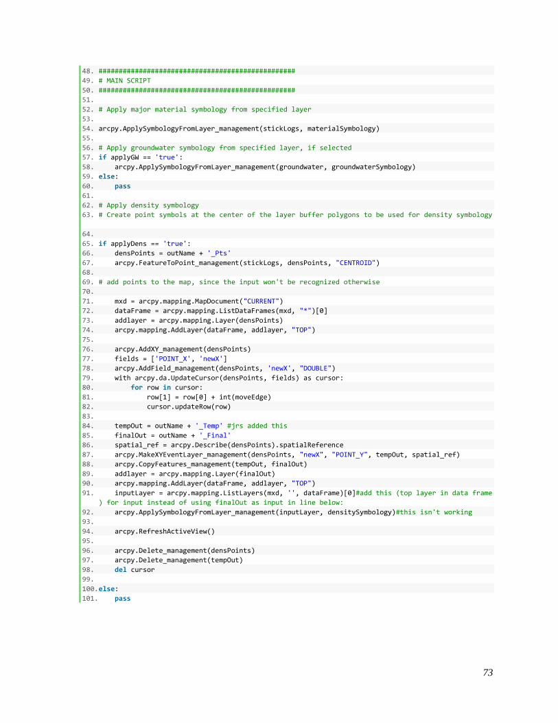
73
48. #################################################
49. # MAIN SCRIPT
50. #################################################
51.
52. # Apply major material symbology from specified layer
53.
54. arcpy.ApplySymbologyFromLayer_management(stickLogs, materialSymbology)
55.
56. # Apply groundwater symbology from specified layer, if selected
57. if applyGW == 'true':
58. arcpy.ApplySymbologyFromLayer_management(groundwater, groundwaterSymbology)
59. else:
60. pass
61.
62. # Apply density symbology
63. # Create point symbols at the center of the layer buffer polygons to be used for density symbology
64.
65. if applyDens == 'true':
66. densPoints = outName + '_Pts'
67. arcpy.FeatureToPoint_management(stickLogs, densPoints, "CENTROID")
68.
69. # add points to the map, since the input won't be recognized otherwise
70.
71. mxd = arcpy.mapping.MapDocument("CURRENT")
72. dataFrame = arcpy.mapping.ListDataFrames(mxd, "*")[0]
73. addlayer = arcpy.mapping.Layer(densPoints)
74. arcpy.mapping.AddLayer(dataFrame, addlayer, "TOP")
75.
76. arcpy.AddXY_management(densPoints)
77. fields = ['POINT_X', 'newX']
78. arcpy.AddField_management(densPoints, 'newX', "DOUBLE")
79. with arcpy.da.UpdateCursor(densPoints, fields) as cursor:
80. for row in cursor:
81. row[1] = row[0] + int(moveEdge)
82. cursor.updateRow(row)
83.
84. tempOut = outName + '_Temp' #jrs added this
85. finalOut = outName + '_Final'
86. spatial_ref = arcpy.Describe(densPoints).spatialReference
87. arcpy.MakeXYEventLayer_management(densPoints, "newX", "POINT_Y", tempOut, spatial_ref)
88. arcpy.CopyFeatures_management(tempOut, finalOut)
89. addlayer = arcpy.mapping.Layer(finalOut)
90. arcpy.mapping.AddLayer(dataFrame, addlayer, "TOP")
91. inputLayer = arcpy.mapping.ListLayers(mxd, '', dataFrame)[0]#add this (top layer in data frame
) for input instead of using finalOut as input in line below:
92. arcpy.ApplySymbologyFromLayer_management(inputLayer, densitySymbology)#this isn't working
93.
94. arcpy.RefreshActiveView()
95.
96. arcpy.Delete_management(densPoints)
97. arcpy.Delete_management(tempOut)
98. del cursor
99.
100. else:
101. pass

74
3. Export to Graphic
1. '''''
2. Description: This scripts exports the current visible extent of an open mxd to a graphic file form
at.
3. The mxd can be in data view or layout view. User can choose resolution parameter (dpi) for all for
mats, and image
4. quality for PDF, AI, and SVG file types.
5.
6.
7. Authors: Jesse Schaefer, Drew Schwitters, Martin Weiser; University of Washington MGIS GEOG569 Cap
stone project
8. '''
9.
10. #import modules
11. import arcpy
12.
13. #parameters
14.
15. file_format = arcpy.GetParameterAsText(0) #pdf, ai, svg, jpg, tiff
16. dpi = arcpy.GetParameterAsText(1) #resolution in dpi
17. quality = arcpy.GetParameterAsText(2) #for pdf, ai, svg only; BEST, BETTER, NORMAL, FASTER, FASTES
T
18. output = arcpy.GetParameterAsText(3)
19.
20. #variables
21.
22. mxd = arcpy.mapping.MapDocument("CURRENT")
23.
24. #############
25. #main script
26. #############
27.
28. try:
29. if file_format == 'pdf':
30. arcpy.mapping.ExportToPDF(mxd, output, resolution = dpi, image_quality = quality)
31. #default pdf resolution is 300
32. elif file_format == 'ai':
33. arcpy.mapping.ExportToAI(mxd, output, resolution = dpi, image_quality = quality)
34. #default pdf resolution is 300
35. elif file_format == 'jpg':
36. arcpy.mapping.ExportToJPEG(mxd, output, resolution = dpi)
37. #default jpeg resolution is 100
38. elif file_format == 'tiff':
39. arcpy.mapping.ExportToTIFF(mxd, output, resolution = dpi)
40. elif file_format == 'svg':
41. arcpy.mapping.ExportToSVG(mxd, output, resolution = dpi, image_quality = quality)
42. arcpy.AddMessage('Exporting to ' + file_format)
43. arcpy.AddMessage('Map was exported to ' + output)
44. except:
45. arcpy.AddMessage('Could not export map to ' + file_format)
46.
47. #cleanup
48. del mxd

75
Appendix C. Toolbox Instructions Document

76
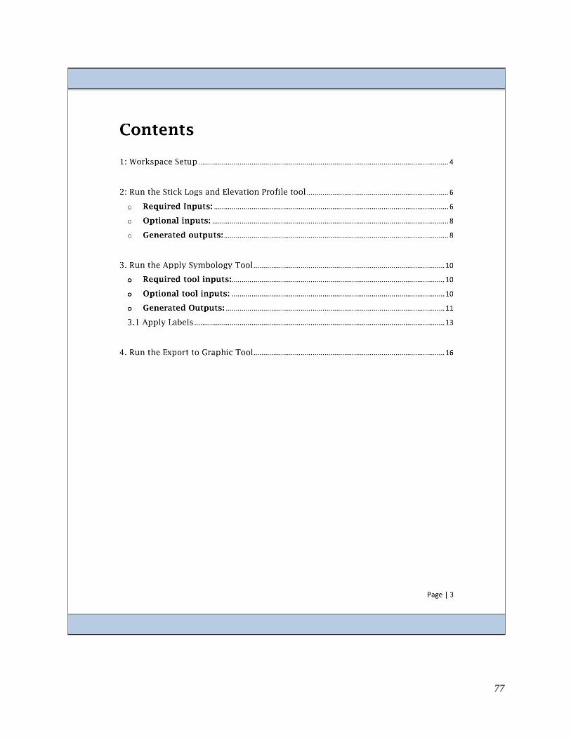
77

78

79
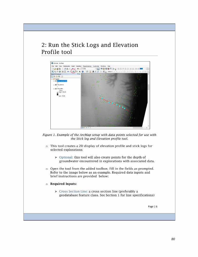
80
81
82

83

84
85

86

87
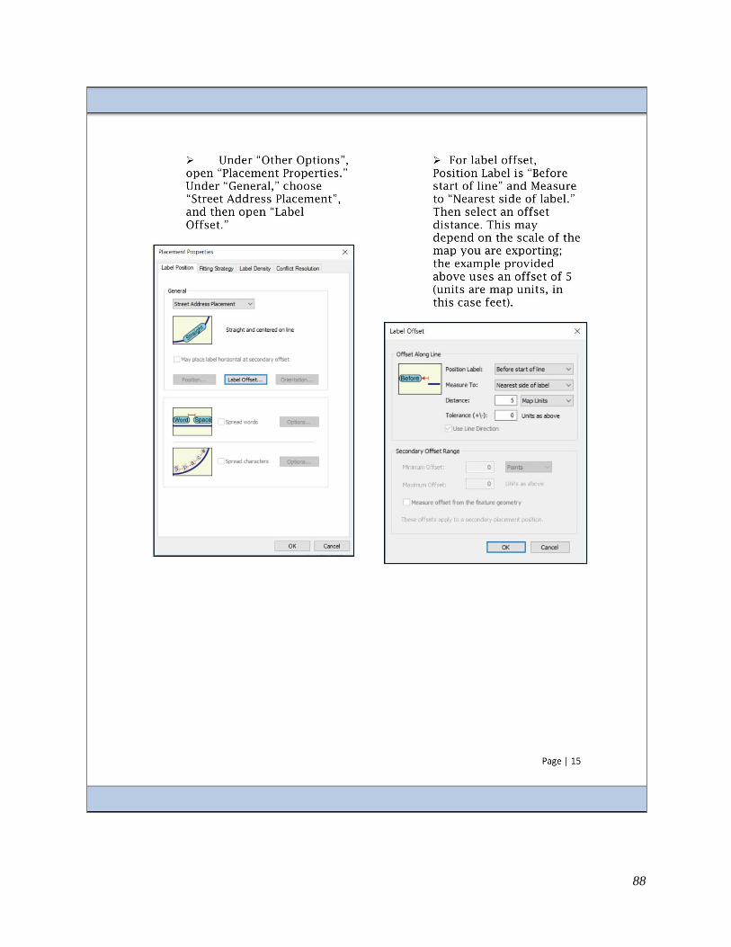
88

89

90
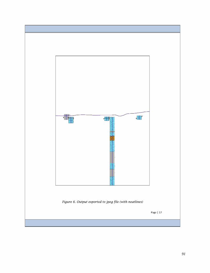
91

92
Appendix D. “Tool parameter documentation” file
Toolbox Name: Geologic Cross Section Toolbox
Parameter Tool Explanation Data Type Script Explanation
1. Stick Logs and Elevation Profile | Script: StickLog&Groundwater&Profile
Cross Section Line Input cross section line layer used
for creating the elevation profile.
This can be an active selection or a
feature class with a single line.
Feature layer linesLayer = arcpy.GetParameterAsText()
transferAtts(inFC, joinTable, parentKey,
childKey, fInfo, outName):
Transfers attributes from a table to a fc: OIDs
must match. Get the attributes through a join
which only works on a feature layer. Make the
join based on key field.
DEM Input bare earth DEM. Raster layer dem = arcpy.GetParameterAsText()
arcpy.InterpolateShape_3d(dem, linesLayer,
zLines)
Interpolate the lines as "z" locations within DEM
for profile line, sticklog, and groundwater.
Start drawing from: Corner of the map from which to
start drawing the profile line and
stick logs.
String cp = getCPValue(arcpy.GetParameterAsText()
getCPValue(quadrant):
Vertical Exaggeration Vertical exaggeration value applied
to the profile line and stick logs.
Double ve = arcpy.GetParameterAsText()
plan2side(ZMlines, ve, he):
Flip map view lines to cross section view without
creating a copy this function updates the existing
geometry.
Horizontal
Exaggeration
Horizontal exaggeration value
applied to the profile line and stick
log spacing.
Double he = arcpy.GetParameterAsText()
plan2side(ZMlines, ve, he):
Flip map view lines to cross section view without
creating a copy this function updates the existing
geometry.
Output Surface Profile Output location and file name for
elevation profile line(s).
Feature class outFC = arcpy.GetParameterAsText()
outName = os.path.splitext()
addAndCalc()
arcpy.InterpolateShape_3d()
arcpy.CreateRoutes_lr()
arcpy.CreateFeatureclass_management()
arcpy.Append_management()
Interpolate the lines, measure the lines, hook the
attributes back up transferAtts(inFC, joinTable,
parentKey, childKey, fInfo, outName), copy the
final fc from the scratch gdb to the output
directory
Selected Explorations Exploration points that will be used
to create stick logs. This can be an
active selection or a feature class
containing just the desired points.
Feature layer bhLayer = arcpy.GetParameterAsText()
arcpy.InterpolateShape_3d()
arcpy.AddField_management()
arcpy.CalculateField_management()
arcpy.LocateFeaturesAlongRoutes_lr()
arcpy.DeleteIdentical_management()
arcpy.CreateRoutes_lr()
arcpy.MakeRouteEventLayer_lr()
arcpy.Select_analysis()
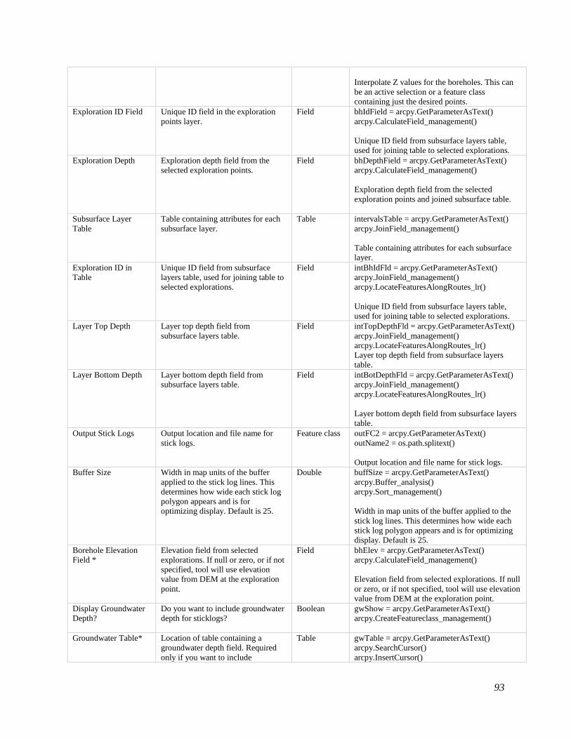
93
Interpolate Z values for the boreholes. This can
be an active selection or a feature class
containing just the desired points.
Exploration ID Field Unique ID field in the exploration
points layer.
Field bhIdField = arcpy.GetParameterAsText()
arcpy.CalculateField_management()
Unique ID field from subsurface layers table,
used for joining table to selected explorations.
Exploration Depth Exploration depth field from the
selected exploration points.
Field bhDepthField = arcpy.GetParameterAsText()
arcpy.CalculateField_management()
Exploration depth field from the selected
exploration points and joined subsurface table.
Subsurface Layer
Table
Table containing attributes for each
subsurface layer.
Table intervalsTable = arcpy.GetParameterAsText()
arcpy.JoinField_management()
Table containing attributes for each subsurface
layer.
Exploration ID in
Table
Unique ID field from subsurface
layers table, used for joining table to
selected explorations.
Field intBhIdFld = arcpy.GetParameterAsText()
arcpy.JoinField_management()
arcpy.LocateFeaturesAlongRoutes_lr()
Unique ID field from subsurface layers table,
used for joining table to selected explorations.
Layer Top Depth Layer top depth field from
subsurface layers table.
Field intTopDepthFld = arcpy.GetParameterAsText()
arcpy.JoinField_management()
arcpy.LocateFeaturesAlongRoutes_lr()
Layer top depth field from subsurface layers
table.
Layer Bottom Depth Layer bottom depth field from
subsurface layers table.
Field intBotDepthFld = arcpy.GetParameterAsText()
arcpy.JoinField_management()
arcpy.LocateFeaturesAlongRoutes_lr()
Layer bottom depth field from subsurface layers
table.
Output Stick Logs Output location and file name for
stick logs.
Feature class outFC2 = arcpy.GetParameterAsText()
outName2 = os.path.splitext()
Output location and file name for stick logs.
Buffer Size Width in map units of the buffer
applied to the stick log lines. This
determines how wide each stick log
polygon appears and is for
optimizing display. Default is 25.
Double buffSize = arcpy.GetParameterAsText()
arcpy.Buffer_analysis()
arcpy.Sort_management()
Width in map units of the buffer applied to the
stick log lines. This determines how wide each
stick log polygon appears and is for optimizing
display. Default is 25.
Borehole Elevation
Field *
Elevation field from selected
explorations. If null or zero, or if not
specified, tool will use elevation
value from DEM at the exploration
point.
Field bhElev = arcpy.GetParameterAsText()
arcpy.CalculateField_management()
Elevation field from selected explorations. If null
or zero, or if not specified, tool will use elevation
value from DEM at the exploration point.
Display Groundwater
Depth?
Do you want to include groundwater
depth for sticklogs?
Boolean gwShow = arcpy.GetParameterAsText()
arcpy.CreateFeatureclass_management()
Groundwater Table* Location of table containing a
groundwater depth field. Required
only if you want to include
Table gwTable = arcpy.GetParameterAsText()
arcpy.SearchCursor()
arcpy.InsertCursor()

94
groundwater depth. arcpy.CreateObject()
arcpy.AddJoin_management()
Creates search cursor insert cursor and creates
object from selected field, joins table with
exploration points.
Groundwater Depth
Field*
Groundwater depth field from
groundwater table . Required only if
you want to include groundwater
depth.
Field gwDepthField = arcpy.GetParameterAsText()
arcpy.CalculateField_management()
Selects groundwater depth field from
groundwater table.
Exploration ID Field
in GW Table*
Unique ID field in the groundwater
table. Required only if you want to
include groundwater depth.
Field bhIdField2 = arcpy.GetParameterAsText()
arcpy.AddJoin_management()
Unique ID field in the groundwater table.
Used to join groundwater table and exploration
points. Required only if you want to include
groundwater depth.
2. Apply Symbology | Script: Symbology
Input Stick Log Buffer
Feature Layer
Feature layer of stick log polygons;
output from Profile and Stick Log
tool.
Feature layer stickLogs = arcpy.GetParameterAsText()
Select feature layer from stick log output
Input MajorMaterial
Symboloy Layer*
Layer file with desired major
material symbology.
Layer file materialSymbology =
arcpy.GetParameterAsText()
arcpy.ApplySymbologyFromLayer_management
()
Select major material layer file
Groundwater Depth
Points Features*
Points feature layer of groundwater
depth locations for stick logs. This is
an output created by the 'Stick Logs
and Elevation Profile' Tool.
Required only if you want to apply
groundwater symbology.
Feature layer groundwater = arcpy.GetParameterAsText()
arcpy.mapping.AddLayer
Select groundwater points output
Groundwater Depth
Symbology Layer*
Layer file with desired groundwater
symbology. Required only if you
want to apply groundwater
symbology.
Layer file groundwaterSymbology =
arcpy.GetParameterAsText()
arcpy.ApplySymbologyFromLayer_management
()
Select groundwater symbology layer file
Input Density
Symbology Layer*
Layer file with desired density
symbology. Required only if you
want to apply density symbology.
Layer file densitySymbology =
arcpy.GetParameterAsText()
Select density layer file
Output Density
Points*
Output file with symbolized density
points; these will display for each
layer along the right side of the stick
log. Required only if you want to
apply density symbology.
Feature class densityOutPoints = arcpy.GetParameterAsText()
outName = os.path.splitext()
Select output file path
Density Symbols
Distance to Buffer
Edge?*
Buffer distance applied to place the
density symbols along the edge of
the stick log. This will depend on the
value chosen for “Buffer Size” in the
Stick Logs and Elevation Profile
tool. A value of several units greater
than that used for Buffer Size is
ideal. Required only if you want to
apply density symbology.
Long moveEdge = arcpy.GetParameterAsText(()
arcpy.FeatureToPoint_management()
arcpy.MakeXYEventLayer_management()
CopyFeatures_management()
Creates a buffer distance from sticklog buffer
output. Select a buffer size that is larger than the
Stocklogs, Elevation Profile, and Groundwater
Tool.
Apply Density?* Check this box if you want to apply
density symbology.
Boolean arcpy.ApplySymbologyFromLayer_management
()
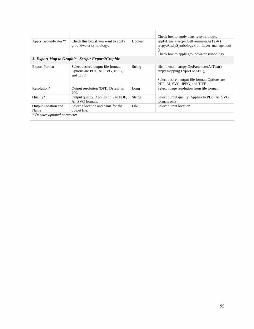
95
Check box to apply density symbology.
Apply Groundwater?* Check this box if you want to apply
groundwater symbology.
Boolean applyDens = arcpy.GetParameterAsText()
arcpy.ApplySymbologyFromLayer_management
()
Check box to apply groundwater symbology.
3. Export Map to Graphic | Script: Export2Graphic
Export Format Select desired output file format.
Options are PDF, AI, SVG, JPEG,
and TIFF.
String file_format = arcpy.GetParameterAsText()
arcpy.mapping.ExportToABC()
Select desired output file format. Options are
PDF, AI, SVG, JPEG, and TIFF.
Resolution* Output resolution (DPI). Default is
200.
Long Select image resolution from file format.
Quality* Output quality. Applies only to PDF,
AI, SVG formats.
String Select output quality. Applies to PDS, AI, SVG
formats only.
Output Location and
Name
Select a location and name for the
output file.
File Select output location.
* Denotes optional parameter