pymses_v3.0.0.pdf - irfu - cea
TRANSCRIPT

PyMSES DocumentationRelease 3.0.0
Thomas GUILLET, Damien CHAPON, Marc LABADENS
February 24, 2012

CONTENTS
1 User’s guide 31.1 PyMSES : Python modules for RAMSES . . . . . . . . . . . . . . . . . . . . . . . . . . . . . . . . 31.2 Installing PyMSES . . . . . . . . . . . . . . . . . . . . . . . . . . . . . . . . . . . . . . . . . . . . 41.3 Get a RAMSES output into PyMSES . . . . . . . . . . . . . . . . . . . . . . . . . . . . . . . . . . 51.4 Reading particles . . . . . . . . . . . . . . . . . . . . . . . . . . . . . . . . . . . . . . . . . . . . . 61.5 AMR data access . . . . . . . . . . . . . . . . . . . . . . . . . . . . . . . . . . . . . . . . . . . . . 91.6 RAMSES AMR file formats . . . . . . . . . . . . . . . . . . . . . . . . . . . . . . . . . . . . . . . 101.7 Dealing with units . . . . . . . . . . . . . . . . . . . . . . . . . . . . . . . . . . . . . . . . . . . . 111.8 Data filtering . . . . . . . . . . . . . . . . . . . . . . . . . . . . . . . . . . . . . . . . . . . . . . . 131.9 Analysis tools . . . . . . . . . . . . . . . . . . . . . . . . . . . . . . . . . . . . . . . . . . . . . . 151.10 Visualization tools . . . . . . . . . . . . . . . . . . . . . . . . . . . . . . . . . . . . . . . . . . . . 19
2 Source documentation 412.1 Data structures and containers . . . . . . . . . . . . . . . . . . . . . . . . . . . . . . . . . . . . . . 412.2 Sources module . . . . . . . . . . . . . . . . . . . . . . . . . . . . . . . . . . . . . . . . . . . . . 452.3 Filters module . . . . . . . . . . . . . . . . . . . . . . . . . . . . . . . . . . . . . . . . . . . . . . 462.4 Analysis module . . . . . . . . . . . . . . . . . . . . . . . . . . . . . . . . . . . . . . . . . . . . . 482.5 Utilities package . . . . . . . . . . . . . . . . . . . . . . . . . . . . . . . . . . . . . . . . . . . . . 57
Module Index 63
Index 65
i

ii

PyMSES Documentation, Release 3.0.0
This is the up-to-date (version 3.0.0) online PyMSES manual.
All the examples presented in this manual are based on RAMSES data available here : RAMSES Data examples.
CONTENTS 1

PyMSES Documentation, Release 3.0.0
2 CONTENTS

CHAPTER
ONE
USER’S GUIDE
1.1 PyMSES : Python modules for RAMSES
1.1.1 Introduction
PyMSES is a set of Python modules originally written for the RAMSES astrophysical fluid dynamics AMR code.
Its purpose :
• provide a clean and easy way of getting the data out of RAMSES simulation outputs.
• help you analyse/manipulate very large simulations transparently, without worrying more than needed aboutdomain decompositions, memory management, etc.,
• interface with a lot of powerful Python libraries (Numpy/Scipy, Matplotlib, PIL, HDF5/PyTables) and existingcode (like your own).
• be a post-processing toolbox for your own data analysis.
What PyMSES is NOT
It is not an interactive environment by itself, but :
• it provides modules which can be used interactively, for example with IPython.
• it also provides an AMRViewer graphical user intergace (GUI) module that allows you to get a quick and easylook at your AMR data.
1.1.2 Documentation
• pdf_manual
• Documentation (HTML)
1.1.3 Contacts
Authors Thomas GUILLET, Damien CHAPON, Marc LABADENS
Contact [email protected], [email protected]
Organization Service d’astrophysique, CEA/Saclay
Address Gif-Sur-Yvette, F91190, France
3

PyMSES Documentation, Release 3.0.0
Date January 03, 2012
1.1.4 Indices and tables
• Index
• Module Index
• Search Page
1.2 Installing PyMSES
1.2.1 Requirements
PyMSES has some Core dependencies plus some Recommended dependencies you might need to install to enable allPyMSES features.
The developpment team strongly recommends the user to install the EPD (Enthought Python Distribution) whichwraps all these dependencies into a single, highly-portable package.
Core dependencies
These packages are mandatory to use the basic functionality of PyMSES:
• a gcc-compatible C compiler,
• GNU make and friends,
• Python, version 2.5.x to 2.6.x (not 3.x), including developement headers (Python.h and such), python 2.6.x isrecommended to use some multiprocessing speed up.
• Python packages:
– numpy, version 1.2 or later
– scipy
• iPython is not strictly required, but it makes the interactive experience so much better you will certainly want toinstall it.
Recommended dependencies
Those packages are recommended for general use (plotting, easy input and output, image processing, GUI, ...). SomePyMSES features may be unavailable without them:
• matplotlib for plotting
• the Python Imaging Library (PIL) for Image processing
• HDF5 and PyTables for Python HDF5 support
• wxPython for the AMRViewer GUI
• mpi4py if you want to use the MPI library on a large parallel system.
4 Chapter 1. User’s guide
PyMSES Documentation, Release 3.0.0
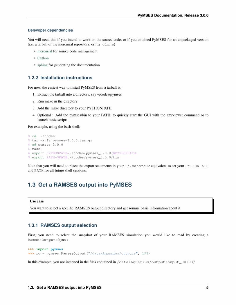
Delevoper dependencies
You will need this if you intend to work on the source code, or if you obtained PyMSES for an unpackaged version(i.e. a tarball of the mercurial repository, or hg clone)
• mercurial for source code management
• Cython
• sphinx for generating the documentation
1.2.2 Installation instructions
For now, the easiest way to install PyMSES from a tarball is:
1. Extract the tarball into a directory, say ~/codes/pymses
2. Run make in the directory
3. Add the make directory to your PYTHONPATH
4. Optional : Add the pymses/bin to your PATH, to quickly start the GUI with the amrviewer command or tolaunch basic scripts.
For example, using the bash shell:
$ cd ~/codes$ tar -xvfz pymses-3.0.0.tar.gz$ cd pymses_3.0.0$ make$ export PYTHONPATH=~/codes/pymses_3.0.0:$PYTHONPATH$ export PATH=$PATH:~/codes/pymses_3.0.0/bin
Note that you will need to place the export statements in your ~/.bashrc or equivalent to set your PYTHONPATHand PATH for all future shell sessions.
1.3 Get a RAMSES output into PyMSES
Use case
You want to select a specific RAMSES output directory and get somme basic information about it
1.3.1 RAMSES output selection
First, you need to select the snapshot of your RAMSES simulation you would like to read by creating aRamsesOutput object :
>>> import pymses>>> ro = pymses.RamsesOutput("/data/Aquarius/outputs", 193)
In this example, you are intersted in the files contained in /data/Aquarius/output/ouput_00193/
1.3. Get a RAMSES output into PyMSES 5

PyMSES Documentation, Release 3.0.0
1.3.2 Ouput information
To get some details about this specific output/simulation. Everything you need is in the info parameter :
>>> ro.info{’H0’: 73.0,’aexp’: 1.0000620502295701,’boxlen’: 1.0,’dom_decomp’: <pymses.sources.ramses.hilbert.HilbertDomainDecomp object at 0x3305e10>,’levelmax’: 18,’levelmin’: 7,’ncpu’: 64,’ndim’: 3,’ngridmax’: 800000,’nstep_coarse’: 9578,’omega_b’: 0.039999999105930301,’omega_k’: 0.0,’omega_l’: 0.75,’omega_m’: 0.25,’time’: 6.2446534480863097e-05,’unit_density’: (2.50416381926e-27 m^-3.kg),’unit_length’: (4.21943976727e+24 m),’unit_mass’: (1.88116596007e+47 kg),’unit_pressure’: (2.50385294276e-13 m^-1.kg.s^-2),’unit_temperature’: (12021826243.9 K),’unit_time’: (4.21970170037e+17 s),’unit_velocity’: (9999379.26156 m.s^-1)}
>>> ro.info["ncpu"]64
>>> ro.info["boxlen"] / 2**ro.info["levelmax"]3.814697265625e-06
This way, you can easily find the units of your data (see Dealing with units).
1.4 Reading particles
1.4.1 Particle data source
If you want to look at the particles, you need to create a RamsesParticleSource. To do so, call theparticle_source() method of your RamsesOutput object with a list of the different fields you might need inyour analysis.
The available fields are :
• “vel” : the velocities of the particles
• “mass” : the mass of the particles
• “id” : the id number of the particles
• “level” : the AMR level of refinement of the cell each particle belongs to
• “epoch” : the birth time of the particles (0.0 for ic particles, >0.0 for star formation particles)
• “metal” : the metallicities of the particles
6 Chapter 1. User’s guide

PyMSES Documentation, Release 3.0.0
>>> ro = pymses.RamsesOutput("/data/Aquarius/output", 193)>>> part = ro.particle_source(["vel", "mass"])
Warning
The data source you just created does not contain data. It is designed to provide an on-demand access to thedata. To be memory-friendly, nothing is read from the disk yet at this point. All the part_00193.out_* filesare only linked to the data source for further processing.
1.4.2 PointDataset
At the opposite, a PointDataset is an actual data container.
Single CPU particle dataset
If you want to read all the particles of the cpu number 3 (written in part_00193.out_00003), use theget_domain_dset() method :
>>> dset3 = part.get_domain_dset(3)Reading particles : /data/Aquarius/output/output_00193/part_00193.out00003
Number of particles
Every PointDataset has a npoints int parameter which gives you the number of particles in this dataset :
>>> print "CPU 3 has %i particles"%dset3.npointsCPU 3 has 157976 particles
Particle coordinates
The points parameter of the PointDataset contains the coordinates of the particles :
>>> print dset3.pointsarray([[ 0.49422911, 0.51383241, 0.50130034],
[ 0.49423128, 0.51374527, 0.50136899],[ 0.49420231, 0.51378629, 0.50190981],...,[ 0.49447162, 0.51394969, 0.50146777],[ 0.49422794, 0.51378071, 0.50176276],[ 0.4946566 , 0.51491008, 0.50117673]])
Particle fields
You also have an easy access to the different fields :
1.4. Reading particles 7
PyMSES Documentation, Release 3.0.0
>>> print dset3["mass"]array([ 4.69471978e-07, 4.69471978e-07, 9.38943957e-07, ...,
4.69471978e-07, 4.69471978e-07, 4.69471978e-07])
1.4.3 Whole data source concatenation
To read all the particles from all the ncpus part_00193.out* files and concatenate them into a single (but maybenot memory-friendly) dataset, call the flatten() method of your part object :
>>> dset_all = part.flatten()Reading particles : /data/Aquarius/output/output_00193/part_00193.out00001Reading particles : /data/Aquarius/output/output_00193/part_00193.out00002Reading particles : /data/Aquarius/output/output_00193/part_00193.out00003Reading particles : /data/Aquarius/output/output_00193/part_00193.out00004
[...]
Reading particles : /data/Aquarius/output/output_00193/part_00193.out00062Reading particles : /data/Aquarius/output/output_00193/part_00193.out00063Reading particles : /data/Aquarius/output/output_00193/part_00193.out00064
>>> print "Domain has %i particles"%dset_all.npointsDomain has 10000000 particles
1.4.4 CPU-by-CPU particles
In most cases, you won’t have enough memory to load all the particles of your simulation domain into a single dataset.You have two different options :
• Filter your particles (see Data filtering).
• Your analysis can be done on a cpu-by-cpu basis. The RamsesParticleSource provides aiter_dsets() iterator yielding cpu-by-cpu datasets :
>>> for dset in part.iter_dsets():print dset.npoints
Reading particles : /data/Aquarius/output/output_00193/part_00193.out00001254210Reading particles : /data/Aquarius/output/output_00193/part_00193.out00002214330Reading particles : /data/Aquarius/output/output_00193/part_00193.out00003359648[...]Reading particles : /data/Aquarius/output/output_00193/part_00193.out00064351203
8 Chapter 1. User’s guide

PyMSES Documentation, Release 3.0.0
1.5 AMR data access
1.5.1 AMR data source
If you want to deal with the AMR data, you need to call the amr_source() method of your RamsesOutputobject with a single argument which is a list of the different fields you might need in your analysis.
When calling the amr_source(), the fields you have access to are :
• “rho” : the gas density field
• “vel” : the gas velocity field
• “P” : the gas pressurre field
• “g” : the gravitational acceleration field
To modify the list of available data fields, see RAMSES AMR file formats.
>>> ro = pymses.RamsesOutput("/data/Aquarius/output", 193)>>> amr = ro.amr_source(["rho", "vel", "P", "g"])
Warning
The data source you just created does not contain data. It is designed to provide an on-demand access to thedata. To be memory-friendly, nothing is read from the disk yet at this point. All the amr_00193.out_*,hydro_00193.out_* and grav_00193.out_* files are only linked to the data source for further pro-cessing.
1.5.2 AMR data handling
AMR data is a bit more complicated to handle than particle data. To perform various analysis, PyMSES provides youwith two different tools to get your AMR data :
• AMR grid to cell list conversion
• AMR field point-sampling
AMR grid to cell list conversion
The CellsToPoints filter converts the AMR tree structure into a IsotropicExtPointDataset containing alist of the AMR grid leaf envelope cells :
• The points parameter of the datasets coming from the generated data source will contain the coordinates of thecell centers.
• These datasets will have an additional get_sizes() method giving you the size of each cell.
>>> from pymses.filters import CellsToPoints>>> cell_source = CellsToPoints(amr)>>> cells = cell_source.flatten()[...]# Cell centers>>> ccenters = cells.points
1.5. AMR data access 9

PyMSES Documentation, Release 3.0.0
# Cell sizes>>> dx = cells.get_sizes()
Warning
As a Filter, the cell_source object you first created is another data provider, it doesn’t contain actual data. Toread the data, use get_domain_dset(), iter_dsets() or flatten() method as described in Readingparticles.
AMR field point-sampling
Another way to read the AMR data is to perform a sampling of the AMR fields with a set of sampling points coordinatesof your choice. In PyMSES, this is done quite easily with the sample_points() function :
>>> from pymses.analysis import sample_points>>> sample_dset = sample_points(amr, points)
The returned sample_dset will be a PointDataset containing all your sampling points and the corresponding valueof the different AMR fields you selected.
Note
In backstage, the point sampling is performed with a tree search algorithm, which makes this particular processof AMR data access both user-friendly and efficient.
For example, this method can be used :
• for visualization purposes (see Slices).
• when computing profiles (see Profile computing)
1.6 RAMSES AMR file formats
1.6.1 Default
The default settings for the AMR data file formats is as follow:
>>> from pymses.sources.ramses.octree import RamsesOctreeReader as ROR>>> ROR.fields_by_file = {... "hydro" : [ ROR.Scalar("rho", 0), ROR.Vector("vel", [1, 2, 3]), ROR.Scalar("P", 4) ],... "grav" : [ ROR.Vector("g", [0, 1, 2]) ]... }
which means that in the hydro_*.out* files :
• the first read variable corresponds to the scalar gas density field
• the next 3 read variables corresponds to the gas 3D velocity field
• the fifth read variable corresponds to the scalar gas pressure field
and in the grav_*.out* files :
10 Chapter 1. User’s guide

PyMSES Documentation, Release 3.0.0
• the 3 read variables corresponds to the 3D gravitational acceleration field
1.6.2 User-defined
If you use a nD (n 6= 3) or a non-standard version of RAMSES, you might want to redefine this AMR file format to :
• make additional tracers available to your reader
• read nD (n 6= 3) data
>>> from pymses.sources.ramses.octree import RamsesOctreeReader as ROR
>>> # 2D data format>>> ROR.fields_by_file = {... "hydro" : [ ROR.Scalar("rho", 0), ROR.Vector("vel", [1, 2]), ROR.Scalar("P", 3) ],... "grav" : [ ROR.Vector("g", [0, 1]) ]... }
>>> # Read additional tracers : metallicity, HCO abundancy>>> ROR.fields_by_file = {... "hydro" : [ ROR.Scalar("rho", 0), ROR.Vector("vel", [1, 2, 3]), ROR.Scalar("P", 4), ROR.Scalar("Z", 5), ROR.Scalar("HCO", 6) ],... "grav" : [ ROR.Vector("g", [0, 1, 2]) ]... }
To take into effect these settings, make sure you define them before any call to amr_source():
>>> from pymses import RamsesOutput>>> from pymses.sources.ramses.octree import RamsesOctreeReader as ROR>>> # 2D data format>>> ROR.fields_by_file = {... "hydro" : [ ROR.Scalar("rho", 0), ROR.Vector("vel", [1, 2, 3]), ROR.Scalar("P", 4), ROR.Scalar("Z", 5) ],... "grav" : [ ROR.Vector("g", [0, 1, 2]) ]... }>>> ro = RamsesOutput("/data/metal_simu/run001", 20)>>> amr = ro.amr_source(["rho", "Z"])
1.7 Dealing with units
Need
Okay, I have read my data quite easily. What are the units of these data ? How do I convert them into human-readable units ?Example : From a RAMSES hydro simulation, I want to convert my density field unit into the H/cc unit.
1.7.1 Dimensional physical constants
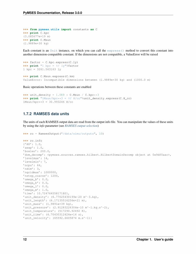
In pymses, a specific module has been designed for this purpose : constants.
It contains a bunch of useful dimensional physical constants (expressed in ISU) which you can use for unit conversionfactors computation, adimensionality tests, etc.
1.7. Dealing with units 11
PyMSES Documentation, Release 3.0.0
>>> from pymses.utils import constants as C>>> print C.kpc(3.085677e+19 m)>>> print C.Msun(1.9889e+30 kg)
Each constant is an Unit instance, on which you can call the express() method to convert this constant intoanother dimension-compatible constant. If the dimensions are not compatible, a ValueError will be raised
>>> factor = C.kpc.express(C.ly)>>> print "1 kpc = %f ly"%factor1 kpc = 3261.563163 ly
>>> print C.Msun.express(C.km)ValueError: Incompatible dimensions between (1.9889e+30 kg) and (1000.0 m)
Basic operations between these constants are enabled
>>> unit_density = 1.0E9 * C.Msun / C.kpc**3>>> print "1Msun/kpc**3 = %f H/cc"%unit_density.express(C.H_cc)1Msun/kpc**3 = 30.993246 H/cc
1.7.2 RAMSES data units
The units of each RAMSES output data are read from the output info file. You can manipulate the values of these unitsby using the info parameter (see RAMSES output selection)
>>> ro = RamsesOutput("/data/simu/outputs", 10)
>>> ro.info{’H0’: 1.0,’aexp’: 1.0,’boxlen’: 200.0,’dom_decomp’: <pymses.sources.ramses.hilbert.HilbertDomainDecomp object at 0x9df0aac>,’levelmax’: 14,’levelmin’: 7,’ncpu’: 64,’ndim’: 3,’ngridmax’: 1000000,’nstep_coarse’: 1200,’omega_b’: 0.0,’omega_k’: 0.0,’omega_l’: 0.0,’omega_m’: 1.0,’time’: 10.724764558171801,’unit_density’: (6.77025430199e-20 m^-3.kg),’unit_length’: (6.17135516256e+21 m),’unit_mass’: (1.9891e+39 kg),’unit_pressure’: (2.91283226304e-10 m^-1.kg.s^-2),’unit_temperature’: (517290.92492 K),’unit_time’: (4.70430312424e+14 s),’unit_velocity’: (65592.6605874 m.s^-1)}
12 Chapter 1. User’s guide

PyMSES Documentation, Release 3.0.0
Assuming you already have sampled the AMR density field of this output into a pdset PointDataset containingall your sampling points (see AMR field point-sampling), you can convert your density field (in code unit) into the unitof your choice:
>>> rho_field_H_cc = pdset["rho"] * ro.info["unit_density"].express(C.H_cc)
Warning
You must take care of manipulating RAMSES data in an unit-coherent way !!!• Good:
>>> info = ro.info
>>> # Density>>> rho_H_cc = rho_ramses * info["unit_density"].express(C.H_cc)
>>> # Mass>>> part_mass_Msun = part_mass * info["unit_mass"].express(C.Msun)
>>> # Kinetic energy>>> factor = (info["unit_mass"] * info["unit_velocity"]**2).express(C.J)>>> kin_energy_J = part_mass * part_vel**2 * factor
• Not so good:
>>> info = ro.info
>>> # Density>>> factor = (info["unit_mass"] / info["unit_length"]**3).express(C.H_cc)>>> rho_H_cc = rho_ramses * factor
>>> # Mass>>> factor = (info["unit_density"]*info["unit_length"]**3).express(C.Msun)>>> part_mass_Msun = part_mass * factor
>>> # Kinetic energy>>> factor = (info["unit_pressure"] * info["unit_length"]**3).express(C.J)>>> kin_energy_J = part_mass * part_vel**2 * factor
1.8 Data filtering
In PyMSES, a Filter is a data source that :
• filter the data coming from an origin data source.
• provides a new data source out of this filtering process.
1.8.1 Region filter
For a lot of analysis, you are often interested in a particular region of your simulation domain, for example :
• spherical region centered on a dark matter halo in a cosmological simulation.
• cylindrical region containing a galactik disk or a cosmological filament.
• ...
1.8. Data filtering 13

PyMSES Documentation, Release 3.0.0
>>> # Region of interest>>> from pymses.utils.regions import Sphere>>> center = [0.5, 0.5, 0.5]>>> radius = 0.1>>> region = Sphere(center, radius)
To filter data source with a region, use the RegionFilter:
>>> from pymses.filters import RegionFilter>>> from pymses import RamsesOutput>>> ro = RamsesOutput("/data/Aquarius/output/", 193)>>> parts = ro.particle_source(["mass"])>>> amr = ro.amr_source(["rho"])
>>> # Particle filtering>>> filt_parts = RegionFilter(region, parts)
>>> # AMR data filtering>>> filt_amr = RegionFilter(region, amr)
Note
The region filters can greatly improve the I/O performance of your analysis process since it doesn’t require toread all the cpu files (of your entire simulation domain) but only those whose domain intersects your region ofinterest.The filtering process occurs not only at the cpu level (as any other Filter) but also in the choice of requiredcpu files.
1.8.2 The CellsToPoints filter
see AMR grid to cell list conversion.
1.8.3 Function filters
You can also define your own function filter. Here an example where only the particles of mass equal to 3 × 10³M�are gathered :
>>> from pymses.filters import PointFunctionFilter>>> from pymses.utils import constants as C
>>> part_source = ro.particle_source(["mass"])
>>> # Stellar disc particles filter : only keep particles of mass = 3000.0 Msun>>> part_mass_Msun = 3.0E3 * C.Msun>>> part_mass_code = part_mass_Msun.express(ro.info["unit_mass"])>>> st_disc_func = lambda dset: (dset["mass"]==part_mass_code)
>>> # Stellar disc particle data source>>> st_disc_parts = PointFunctionFilter(st_disc_func, part_source)
14 Chapter 1. User’s guide

PyMSES Documentation, Release 3.0.0
1.8.4 Randomly decimated data
You can use the PointRandomDecimatedFilter filter to pick up only a given fraction of points (randomlychosen) from your point-based data:
>>> from pymses.filters import PointRandomDecimatedFilter>>> part_source = ro.particle_source(["mass"])
>>> # Pick up 10 % of the particles>>> fraction = 0.1>>> dec_parts = PointRandomDecimatedFilter(fraction, part_source)
1.8.5 Combining filters
You can pile up as many filters as you want to get the particular data you’re interested in:
>>> # Region filter>>> reg_parts = RegionFilter(region, parts)
>>> # Stellar disc filter>>> st_disc_parts = PointFunctionFilter(st_disc_func, reg_parts)
>>> # 10 % randomly decimated filter>>> dec_parts = PointRandomDecimatedFilter(fraction, st_disc_parts)
In this example, the dec_parts data source will provide you 10% of the stellar particles contained within a given region
1.9 Analysis tools
1.9.1 Profile computing
In this section are presented 2 examples of profile computing. The first is based on AMR data and the second onparticles data.
Cylindrical profile of an AMR scalar field
Use case
You want to compute the cylindrical profile (for example, the surface density of a galactic disk) of a scalar AMRfield (here, the rho density field). We assume that we know beforehand the configuration of the disk (center,radius, thickness, normal vector).
We take the configuration of the galactic disk to be:
>>> gal_center = [ 0.567811, 0.586055, 0.559156 ] # in box units>>> gal_radius = 0.00024132905460547268 # in box units>>> gal_thickn = 0.00010238202316595811 # in box units>>> gal_normal = [ -0.172935, 0.977948, -0.117099 ] # Norm = 1
1.9. Analysis tools 15

PyMSES Documentation, Release 3.0.0
Reading AMR data from the RAMSES output
As already explained in Get a RAMSES output into PyMSES and AMR data access, we create the AMR data sourcefrom the RAMSES output we are intersted in, reading only the density field:
>>> from pymses import RamsesOutput>>> output = RamsesOutput("/data/Aquarius/output", 193)# Prepare to read the density field only>>> source = output.amr_source(["rho"])
Random sampling of the AMR data fields in a given region of interest
Now we build the Cylinder that will define the region of interest for the profile:
>>> from pymses.utils.regions import Cylinder>>> cyl = Cylinder(gal_center, gal_normal, gal_radius, gal_thickn)
Generation of an array of 106 random points uniformly spread within the cylinder (random_points() function),and then sampling of the AMR fields at these coordinates (see AMR field point-sampling):
>>> from pymses.analysis import sample_points>>> points = cyl.random_points(1.0e6) # 1M sampling points>>> point_dset = sample_points(source, points)
Computing the profile from the point-based samples
As we are interested in the density profile, we use the data field rho as the weight function. We also take 200 linearlyspaced radial bins within the cylinder radius:
>>> import numpy>>> rho_weight_func = lambda dset: dset["rho"]>>> r_bins = numpy.linspace(0.0, gal_radius, 200)
Now we compute the profile of the resulting PointDataset using the bin_cylindrical() function.
We set the divide_by_counts flag to True, because we’re averaging the density field in each cylindrical shell:
>>> from pymses.analysis import bin_cylindrical>>> rho_profile = bin_cylindrical(point_dset, gal_center, gal_normal,... rho_weight_func, r_bins, divide_by_counts=True)
Finally, we can plot the profile with Matplotlib:
16 Chapter 1. User’s guide

PyMSES Documentation, Release 3.0.0
Spherical profile of a set of particle data
Use case
You want to compute the spherical radial profile of a given particle data field.Example : From a RAMSES cosmological simulation, you want to compute the radial density profile of a darkmatter halo. You already know the position and the size of the halo.
We take the location and spatial extension of the dark matter halo to be:
>>> halo_center = [ 0.567811, 0.586055, 0.559156 ] # in box units>>> halo_radius = 0.00075 # in box units
Reading particle data from a RAMSES output
As already explained in Get a RAMSES output into PyMSES and Reading particles, we create the particle data sourcefrom the RAMSES output we are intersted in, reading only the mass and epoch fields:
1.9. Analysis tools 17

PyMSES Documentation, Release 3.0.0
>>> from pymses import RamsesOutput>>> ro = RamsesOutput("/data/Aquarius/output", 193)# Prepare to read the mass/epoch fields only>>> source = ro.particle_source(["mass", "epoch"])
Filtering all the initial particles within a given region of interest
See Data filtering for details.
Now we build the Sphere that will define the region of interest for the profile:
>>> from pymses.utils.regions import Sphere>>> sph = Sphere(halo_center, halo_radius)
Then filter all the particles contained in the sphere by using a RegionFilter:
>>> from pymses.filters import RegionFilter>>> point_dset = RegionFilter(sph, source)
Filter all the particles which are initially present in the simulation using a PointFunctionFilter:
>>> from pymses.filters import PointFunctionFilter>>> dm_filter = lambda dset: dset["epoch"] == 0.0>>> dm_parts = PointFunctionFilter(dm_filter, point_dset)
Computing the profile
As we are interested in the density profile, we use the data field mass as the weight function. We also take 200 linearlyspaced radial bins within the sphere radius:
>>> import numpy>>> m_weight_func = lambda dset: dset["mass"]>>> r_bins = numpy.linspace(0.0, halo_radius, 200)
Now we compute the profile bin_spherical() function.
We set the divide_by_counts flag to False (optional, this is the default value), because we’re cumulating the massesof the particles in spherical shells:
>>> from pymses.analysis import bin_spherical>>> # This triggers the actual reading of the particle data files from disk.>>> mass_profile = bin_spherical(dm_parts, halo_center, m_weight_func, r_bins, divide_by_counts=False)
To compute the density profile, we divide the mass profile by the volume of each spherical shell:
>>> sph_vol = 4.0/3.0 * numpy.pi * r_bins**3>>> shell_vol = numpy.diff(sph_vol)>>> rho_profile = mass_profile / shell_vol
18 Chapter 1. User’s guide

PyMSES Documentation, Release 3.0.0
1.10 Visualization tools
1.10.1 Camera and Operator
Camera
To do some data visualization, the view parameters are handled by a Camera:
>>> from pymses.analysis.visualization import Camera>>> cam = Camera(center=[0.5, 0.5, 0.5], line_of_sight_axis=’z’, region_size=[0.5, 0.5], distance=0.5,... far_cut_depth=0.5, up_vector=’y’, map_max_size=512, log_sensitive=True)
This object is then used in every PyMSES visualization tool to render an image from the data.
The camera is :
• centered around center
• oriented according to a line_of_sight_axis pointing towards the observer and an up_vector pointing upwards(in the camera plane)
1.10. Visualization tools 19
PyMSES Documentation, Release 3.0.0
• delimited by a region_size in the directions perpendicular to the camera plane.
• delimited by front/background cut planes at position distance/far_cut_depth along the line-of-sight axis
• log-sensitive or not (log_sensitive)
• built with a virtual CCD-detector matrix of max. size map_max_size
Saving / loading a Camera
Camera can be saved into an HDF5 file:
>>> import tables>>> from pymses.analysis.visualization import Camera>>> cam = Camera(center=[0.5, 0.5, 0.8], line_of_sight_axis=’y’, region_size=[0.5, 0.8], distance=0.2)>>> file= tables.openFile("my_cam.hdf5", "w")>>> cam.save_HDF5(file)
It can also be loaded from a HDF5 file to retrieve a previous view:
>>> import tables>>> from pymses.analysis.visualization import Camera>>> file= tables.openFile("my_cam.hdf5", "r")>>> cam = Camera.from_HDF5(file)
Other utility functions
The camera definition can be used to know the maximum Ramses AMR level up needed to compute the image map:
>>> level_max = cam.get_required_resolution()
To do further computation we can also get the pixel surface from the camera object:
>>> pixel_surface = cam.get_pixel_surface()
We can get some camera oriented slice points directly from the camera (see Slices):
>>> slice_points = cam.get_slice_points(z)
Operator
For every PyMSES visualization method you might use, you must define the physical scalar quantity you are interestedin.
For example, you can describe the kinetic energy of particles with the ScalarOperator:
>>> import numpy>>> from pymses.analysis.visualization import ScalarOperator>>> def kin_en_func(dset):... m = dset["mass"]... v2 = numpy.sqrt(numpy.sum(dset["vel"]**2, axis=1))... return m*v2>>> Ek = ScalarOperator(kin_en_func)
20 Chapter 1. User’s guide

PyMSES Documentation, Release 3.0.0
You can also define FractionOperator. For example, if you need a mass-weighted temperature operator for yourAMR grid (FFT-maps):
>>> from pymses.analysis.visualization import FractionOperator>>> M_func = lambda dset: dset["rho"] * dset.get_sizes()**3>>> def num(dset):... T = dset["P"]/dset["rho"]... M = M_func(dset)... return T * M>>> op = FractionOperator(num, M_func)
If you want to ray-trace the max. AMR level of refinement along the line-of-sight, use MaxLevelOperator.
1.10.2 Maps
Slices
Intro
A quick way to look at data is to compute 2D data slice map.
Here is how it works: It first gets some sample points from a camera object, using a basic 2D Cartesian grid. Thenthose points are evaluated using the pymses point_sampler module. A sampling operator can eventually be applied onthe data.
Example
We first need to define a suitable camera:
>>> from pymses.analysis.visualization import Camera>>> cam = Camera(center=[0.5, 0.5, 0.5], line_of_sight_axis=’z’, region_size=[1., 1.],\... up_vector=’y’, map_max_size=512, log_sensitive=True)
Using the amr data previously defined in AMR data access, we can get the map corresponding to the defined sliceview. A logarithmic scale is here applied as it is defined in the camera object.
>>> from pymses.analysis.visualization import SliceMap, ScalarOperator>>> rho_op = ScalarOperator(lambda dset: dset["rho"])>>> map = SliceMap(amr, cam, rho_op, z=0.4) # create a density slice map at z=0.4 depth position
The result can be seen using the matplotlib library:
>>> import pylab as P>>> P.imshow(map)>>> P.show()
1.10. Visualization tools 21

PyMSES Documentation, Release 3.0.0
FFT-convolved maps
Intro
A very simple, fast and accurate data projection (3D->2D) method : each particle/AMR cell is convolved by a 2Dgaussian kernel (Splatter) which size depends on the local AMR grid level.
The convolution of the binned particles/AMR cells histogram with the gaussian kernels is performed with FFT tech-niques by a MapFFTProcessor. You can see two examples of this method below :
• Particles map
• AMR data map
Important note on operators
You must keep in mind that any X Operator you use with this method must describe an extensive physicalvariable since this method compute a summation over particle/AMR quantities :map[i, j] =
∑particles/AMR cells
X
22 Chapter 1. User’s guide

PyMSES Documentation, Release 3.0.0
Examples
Particles map
from numpy import array, log10import pylabfrom pymses.analysis.visualization import *from pymses import RamsesOutputfrom pymses.utils import constants as C
# Ramses dataioutput = 193ro = RamsesOutput("/data/Aquarius/output/", ioutput)parts = ro.particle_source(["mass", "level"])
# Map operator : massscal_func = ScalarOperator(lambda dset: dset["mass"])
# Map regioncenter = [ 0.567811, 0.586055, 0.559156 ]axes = {"los": array([ -0.172935, 0.977948, -0.117099 ])}
# Map processingmp = fft_projection.MapFFTProcessor(parts, ro.info)for axname, axis in axes.items():
cam = Camera(center=center, line_of_sight_axis=axis, up_vector="z", region_size=[5.0E-1, 4.5E-1], \distance=2.0E-1, far_cut_depth=2.0E-1, map_max_size=512)
S = cam.get_pixel_surface()map = mp.process(scal_func, cam, surf_qty=True)factor = (ro.info["unit_mass"]/ro.info["unit_length"]**2).express(C.Msun/C.kpc**2)scale = ro.info["unit_length"].express(C.Mpc)
# pylab.imshow(map)# pylab.show()
# Save map into HDF5 filemapname = "DM_Sigma_%s_%5.5i"%(axname, ioutput)h5fname = save_map_HDF5(map, cam, map_name=mapname)
# Plot map into Matplotlib figure/PIL Imagefig = save_HDF5_to_plot(h5fname, map_unit=("$M_{\odot}.kpc^{-2}$",factor), axis_unit=("Mpc", scale), cmap="Blues", fraction=0.1)
# pil_img = save_HDF5_to_img(h5fname, cmap="Blues", fraction=0.1)
# Save map into PNG image file# save_HDF5_to_plot(h5fname, map_unit=("$M_{\odot}.kpc^{-2}$",factor), \# axis_unit=("Mpc", scale), img_path="./", cmap="Blues", fraction=0.1)# save_HDF5_to_img(h5fname, img_path="./", cmap="Blues", fraction=0.1)
# pylab.show()
1.10. Visualization tools 23

PyMSES Documentation, Release 3.0.0
AMR data map
from numpy import arrayimport pylabfrom pymses.analysis.visualization import *from pymses import RamsesOutputfrom pymses.utils import constants as C
# Ramses dataioutput = 193ro = RamsesOutput("/data/Aquarius/output/", ioutput)amr = ro.amr_source(["rho", "P"])
# Map operator : mass-weighted density mapup_func = lambda dset: (dset["rho"]**2 * dset.get_sizes()**3)down_func = lambda dset: (dset["rho"] * dset.get_sizes()**3)scal_func = FractionOperator(up_func, down_func)
# Map regioncenter = [ 0.567811, 0.586055, 0.559156 ]axes = {"los": array([ -0.172935, 0.977948, -0.117099 ])}
24 Chapter 1. User’s guide

PyMSES Documentation, Release 3.0.0
# Map processingmp = fft_projection.MapFFTProcessor(amr, ro.info)for axname, axis in axes.items():
cam = Camera(center=center, line_of_sight_axis=axis, up_vector="z", region_size=[5.0E-1, 4.5E-1], \distance=2.0E-1, far_cut_depth=2.0E-1, map_max_size=512)
map = mp.process(scal_func, cam)factor = ro.info["unit_density"].express(C.H_cc)scale = ro.info["unit_length"].express(C.Mpc)
# pylab.imshow(map)# Save map into HDF5 filemapname = "gas_mw_%s_%5.5i"%(axname, ioutput)h5fname = save_map_HDF5(map, cam, map_name=mapname)
# Plot map into Matplotlib figure/PIL Imagefig = save_HDF5_to_plot(h5fname, map_unit=("H/cc",factor), axis_unit=("Mpc", scale), cmap="jet")
# pil_img = save_HDF5_to_img(h5fname, cmap="jet")
# Save into PNG image file# save_HDF5_to_plot(h5fname, map_unit=("H/cc",factor), axis_unit=("Mpc", scale), img_path="./", cmap="jet")# save_HDF5_to_img(h5fname, img_path="./", cmap="jet")
# pylab.show()
1.10. Visualization tools 25

PyMSES Documentation, Release 3.0.0
Ray-traced maps
Intro
Ray-traced maps are computed in PyMSES by integrating a physical quantity along rays, each one corresponding to apixel of the map. Ray-tracing is handled by a RayTracer. You can see two examples of this method below :
• Density map
• Min. temperature map
• Max. AMR level of refinement map
Important note on operators
You must keep in mind that any X Operator you use with this method must describe an intensive physicalvariable since this method compute an integral of an AMR quantity over each pixel surface and along the line-of-sight :
map[i, j] =
∫ zmax
zmin
XdSpixdz
Examples
Density map
from numpy import arrayimport pylabfrom pymses.analysis.visualization import *from pymses import RamsesOutputfrom pymses.utils import constants as C
# Ramses dataioutput = 193ro = RamsesOutput("/data/Aquarius/output/", ioutput)
# Map operator : mass-weighted density mapup_func = lambda dset: (dset["rho"]**2)down_func = lambda dset: (dset["rho"])scal_op = FractionOperator(up_func, down_func)
# Map regioncenter = [ 0.567811, 0.586055, 0.559156 ]axes = {"los": array([ -0.172935, 0.977948, -0.117099 ])}
# Map processingrt = raytracing.RayTracer(ro, ["rho"])for axname, axis in axes.items():
cam = Camera(center=center, line_of_sight_axis=axis, up_vector="z", region_size=[3.0E-2, 3.0E-2], \distance=2.0E-2, far_cut_depth=2.0E-2, map_max_size=512)
map = rt.process(scal_op, cam)factor = ro.info["unit_density"].express(C.H_cc)scale = ro.info["unit_length"].express(C.Mpc)
# Save map into HDF5 filemapname = "gas_rt_mw_%s_%5.5i"%(axname, ioutput)
26 Chapter 1. User’s guide

PyMSES Documentation, Release 3.0.0
h5fname = save_map_HDF5(map, cam, map_name=mapname)
# Plot map into Matplotlib figure/PIL Imagefig = save_HDF5_to_plot(h5fname, map_unit=("H/cc",factor), axis_unit=("Mpc", scale), cmap="jet")
# pil_img = save_HDF5_to_img(h5fname, cmap="jet")
# Save into PNG image file# save_HDF5_to_plot(h5fname, map_unit=("H/cc",factor), axis_unit=("Mpc", scale), img_path="./", cmap="jet")# save_HDF5_to_img(h5fname, img_path="./", cmap="jet")
#pylab.show()
Min. temperature map
from numpy import array, zeros_likeimport pylabfrom pymses.analysis.visualization import *from pymses import RamsesOutputfrom pymses.utils import constants as C
# Ramses dataioutput = 193
1.10. Visualization tools 27

PyMSES Documentation, Release 3.0.0
ro = RamsesOutput("/data/Aquarius/output/", ioutput)
# Map operator : minimum temperature along line-of-sightclass MyTempOperator(Operator):
def __init__(self):def invT_func(dset):
P = dset["P"]rho = dset["rho"]r = rho/P
# print r[(rho<=0.0)+(P<=0.0)]# r[(rho<=0.0)*(P<=0.0)] = 0.0
return rd = {"invTemp": invT_func}Operator.__init__(self, d, is_max_alos=True)
def operation(self, int_dict):map = int_dict.values()[0]mask = (map == 0.0)mask2 = map != 0.0map[mask2] = 1.0 / map[mask2]map[mask] = 0.0return map
scal_op = MyTempOperator()
# Map regioncenter = [ 0.567111, 0.586555, 0.559156 ]axes = {"los": "z"}
# Map processingrt = raytracing.RayTracer(ro, ["rho", "P"])for axname, axis in axes.items():
cam = Camera(center=center, line_of_sight_axis=axis, up_vector="y", region_size=[3.0E-3, 3.0E-3], \distance=1.5E-3, far_cut_depth=1.5E-3, map_max_size=512)
map = rt.process(scal_op, cam)factor = ro.info["unit_temperature"].express(C.K)scale = ro.info["unit_length"].express(C.Mpc)
# Save map into HDF5 filemapname = "gas_rt_Tmin_%s_%5.5i"%(axname, ioutput)h5fname = save_map_HDF5(map, cam, map_name=mapname)
# Plot map into Matplotlib figure/PIL Imagefig = save_HDF5_to_plot(h5fname, map_unit=("K",factor), axis_unit=("Mpc", scale), cmap="hot", fraction=0.0)
# pil_img = save_HDF5_to_img(h5fname, cmap="hot")
# Save into PNG image file# save_HDF5_to_plot(h5fname, map_unit=("K",factor), axis_unit=("Mpc", scale), img_path="./", cmap="hot")# save_HDF5_to_img(h5fname, img_path="./", cmap="hot")
#pylab.show()
28 Chapter 1. User’s guide

PyMSES Documentation, Release 3.0.0
Max. AMR level of refinement map
from numpy import arrayimport pylabfrom pymses.analysis.visualization import *from pymses import RamsesOutputfrom pymses.utils import constants as C
# Ramses dataioutput = 193ro = RamsesOutput("/data/Aquarius/output/", ioutput)
# Map operator : max. AMR level of refinement along the line-of-sightscal_op = MaxLevelOperator()
# Map regioncenter = [ 0.567811, 0.586055, 0.559156 ]axes = {"los": array([ -0.172935, 0.977948, -0.117099 ])}
# Map processingrt = raytracing.RayTracer(ro, ["rho"])for axname, axis in axes.items():
1.10. Visualization tools 29

PyMSES Documentation, Release 3.0.0
cam = Camera(center=center, line_of_sight_axis=axis, up_vector="z", region_size=[4.0E-2, 4.0E-2], \distance=2.0E-2, far_cut_depth=2.0E-2, map_max_size=512, log_sensitive=False)
map = rt.process(scal_op, cam)scale = ro.info["unit_length"].express(C.Mpc)
# Save map into HDF5 filemapname = "gas_rt_lmax_%s_%5.5i"%(axname, ioutput)h5fname = save_map_HDF5(map, cam, map_name=mapname)
# Plot map into Matplotlib figure/PIL Imagefig = save_HDF5_to_plot(h5fname, map_unit=("AMR level",1.0), axis_unit=("Mpc", scale), cmap="jet", discrete=True)
# pil_img = save_HDF5_to_img(h5fname, cmap="jet", discrete=True)
# Save into PNG image file# save_HDF5_to_plot(h5fname, map_unit=("AMR level",1.0), axis_unit=("Mpc", scale), img_path="./", cmap="jet", discrete=True)# save_HDF5_to_img(h5fname, img_path="./", cmap="jet", discrete=True)
#pylab.show()
30 Chapter 1. User’s guide
PyMSES Documentation, Release 3.0.0
Multiprocessing
If you are using python 2.6 or higher, the RayTracer will try to use multiprocessing speed up. You candesactivate it to save RAM memory and processor use by setting the multiprocessing option to False:
>>> map = rt.process(scal_op, cam, multiprocessing = False)
1.10.3 AMRViewer GUI
Starting the GUI
PyMSES has a Graphical User Interface (GUI) module which can be used to navigate into AMR data. Once installedas described in Installing PyMSES, the GUI can be started with the following python prompt commands:
>>> from pymses.analysis.visualization import AMRViewer>>> AMRViewer.run()
Loading AMR data
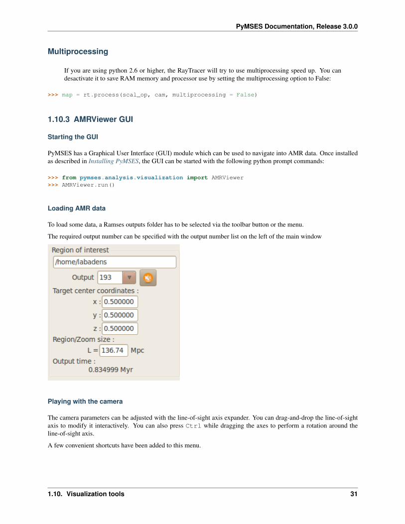
To load some data, a Ramses outputs folder has to be selected via the toolbar button or the menu.
The required output number can be specified with the output number list on the left of the main window
Playing with the camera
The camera parameters can be adjusted with the line-of-sight axis expander. You can drag-and-drop the line-of-sightaxis to modify it interactively. You can also press Ctrl while dragging the axes to perform a rotation around theline-of-sight axis.
A few convenient shortcuts have been added to this menu.
1.10. Visualization tools 31

PyMSES Documentation, Release 3.0.0
There is a possibility to save and load camera parameter via the Camera menu bar.
32 Chapter 1. User’s guide
PyMSES Documentation, Release 3.0.0
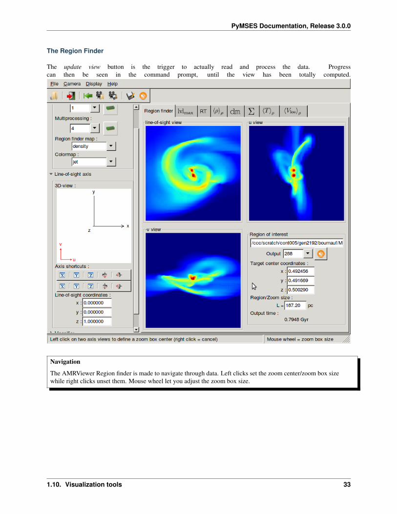
The Region Finder
The update view button is the trigger to actually read and process the data. Progresscan then be seen in the command prompt, until the view has been totally computed.
Navigation
The AMRViewer Region finder is made to navigate through data. Left clicks set the zoom center/zoom box sizewhile right clicks unset them. Mouse wheel let you adjust the zoom box size.
1.10. Visualization tools 33

PyMSES Documentation, Release 3.0.0
Other map types, other tabs
Some other map types can be processed and seen through other tabs as suggested in the display menu:
For example, gas surface density projected map (see FFT-convolved maps):
34 Chapter 1. User’s guide
PyMSES Documentation, Release 3.0.0
1.10. Visualization tools 35

PyMSES Documentation, Release 3.0.0
Mass weighted gas density map (see FFT-convolved maps):Max. AMR level of refinement along the line-of-sight map (see Ray-traced maps):
36 Chapter 1. User’s guide

PyMSES Documentation, Release 3.0.0
1.10. Visualization tools 37

PyMSES Documentation, Release 3.0.0
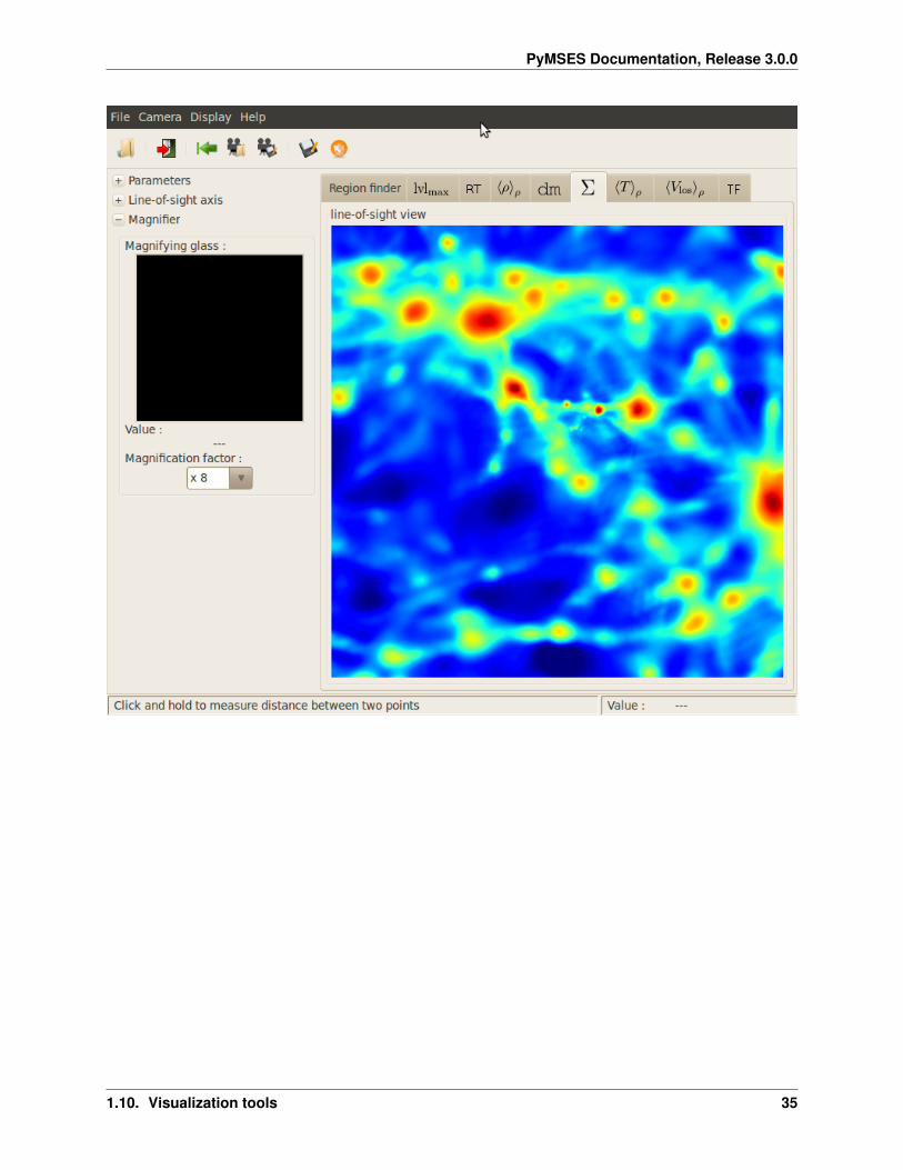
Magnifier
The magnifying glass tool can then be used to see the exact value on the map:
38 Chapter 1. User’s guide

PyMSES Documentation, Release 3.0.0
Rule
The rule tool can be used to measure distances on the maps (click-and-drag behavior):
1.10. Visualization tools 39

PyMSES Documentation, Release 3.0.0
40 Chapter 1. User’s guide

CHAPTER
TWO
SOURCE DOCUMENTATION
2.1 Data structures and containers
2.1.1 pymses.core.sources — PyMSES generic data source module
class Source()Bases: object
Base class for all data source objects
flatten()Read each data file and concatenate resulting dsets. Try to use multiprocessing if possible.
Returns fdset : flattened dataset
iter_dsets()Datasets iterator method. Yield datasets from the datasource
set_read_lmax(max_read_level)Sets the maximum AMR grid level to read in the datasource
Parameters max_read_level : int
max. AMR level to read
class Filter(source)Bases: pymses.core.sources.Source
Data source filter generic class.
filtered_dset(dset)Abstract filtered_dset() method
get_domain_dset(idomain, fields_to_read=None)Get the filtered result of self.source.get_domain_dset(idomain)
Parameters idomain : int
number of the domain from which the data is required
Returns dset : Dataset
the filtered dataset corresponding to the given idomain
get_source_type()
Returns type : int
the result of the get_source_type() method of the source param.
41

PyMSES Documentation, Release 3.0.0
set_read_lmax(max_read_level)Source inherited behavior + apply the set_read_lmax() method to the source param.
Parameters max_read_level : int
max. AMR level to read
class SubsetFilter(data_sublist, source)Bases: pymses.core.sources.Filter
SubsetFilter class. Selects a subset of datasets to read from the datasource
Parameters data_sublist : list of int
list of the selected dataset index to read from the datasource
2.1.2 pymses.core.datasets — PyMSES generic dataset module
class Dataset()Bases: pymses.core.sources.Source
Base class for all dataset objects
add_scalars(name, data)Scalar field addition method
Parameters name : string
human-readable name of the scalar field to add
data : array
raw data array of the new scalar field
add_vectors(name, data)Vector field addition method
Parameters name : string
human-readable name of the vector field to add
data : array
raw data array of the new vector field
fieldsDictionary of the fields in the dataset
class from_hdf5(h5file, where=’/’, close_at_end=False)
iter_dsets()Returns an iterator over itself
write_hdf5(h5file, where=’/’, close_at_end=False)
class PointDataset(points)Bases: pymses.core.datasets.Dataset
Point-based dataset base class
class concatenate(dsets, reorder_indices=None)Datasets concatenation class method. Return a new dataset
Parameters dsets : list of PointDataset
list of all datasets to concatenate
42 Chapter 2. Source documentation
PyMSES Documentation, Release 3.0.0
reorder_indices : array of int (default to None)
particles reordering indices
Returns dset : the new created concatenated PointDataset
filtered_by_mask(mask_array)Datasets filter method. Return a new dataset
Parameters mask_array : numpy.array of numpy.bool
filter mask
Returns dset : the new created filtered PointDataset
class from_hdf5(h5file, where=’/’)
reorder_points(reorder_indices)Datasets reorder method. Return a new dataset
Parameters reorder_indices : array of int
points order indices
Returns dset : the new created reordered PointDataset
transform(xform)Transform the dataset according to the given xform Transformation
Parameters xform : Transformation
write_hdf5(h5file, where=’/’)
class IsotropicExtPointDataset(points, sizes=None)Bases: pymses.core.datasets.PointDataset
Extended point dataset class
get_sizes()
Returns sizes : array
point sizes array
2.1.3 Dataset transformations
pymses.core.transformations Geometrical transformations module
class Transformation()Bases: object
Base class for all geometric transformations acting on Numpy arrays
inverse()Returns the inverse transformation
transform_points(coords)Abstract method. Returns transformed coordinates.
Parameters:
coords – a Numpy array with data points along axis 0 and coordinates along axis 1+
2.1. Data structures and containers 43

PyMSES Documentation, Release 3.0.0
transform_vectors(vectors, coords)Abstract method. Returns transformed vector components for vectors attached to the provided coordinates.
Parameters:
vectors – a Numpy array of shape (ndata, ndim) containing the vector components
coords – a Numpy array of shape (ndata, ndim) containing the point coordinates
class AffineTransformation(lin_xform, shift)Bases: pymses.core.transformations.Transformation
An affine transformation (of the type x -> L(x) + shift)
inverse()Inverse of an affine transformation
transform_points(coords)Apply the affine transformation to coordinates
transform_vectors(vectors, coords)Apply the affine transformation to vectors
class LinearTransformation(matrix)Bases: pymses.core.transformations.Transformation
A generic (matrix-based) linear transformation
inverse()Inverse of the linear transformation
transform_points(coords)Applies a linear transformation to coordinates
transform_vectors(vectors, coords)Applies a linear transformation to vectors
class ChainTransformation(xform_seq)Bases: pymses.core.transformations.Transformation
Defines the composition of a list of transformations
inverse()Inverse of a chained transformation
transform_points(coords)Applies a chained transformation to coordinates
transform_vectors(vectors, coords)Applies a chained transformation to vectors
identity(n)
Returns the identity as a LinearTransformation object :
translation(vect)
Returns an AffineTransformation object corresponding to a translation :
of the specified vector :
rot3d_axvector_matrix(axis_vect, angle)Returns the rotation matrix of the rotation with the specified axis vector and angle
44 Chapter 2. Source documentation

PyMSES Documentation, Release 3.0.0
rot3d_axvector(axis_vect, angle, rot_center=None)Returns the Transformation corresponding to the rotation specified by its axis vector, angle, and rotation center.
If rot_center is not specified, it is assumed to be [0, 0, 0].
rot3d_euler(axis_sequence, angles, rot_center=None)Returns the Transformation corresponding to the rotation specified by its Euler angles and the correspondingaxis sequence convention.
The rotation is performed by successively rotating the object around its current local axis axis_sequence[i] withan angle angle[i], for i = 0, 1, 2.
See http://en.wikipedia.org/wiki/Euler_angles for details.
rot3d_align_vectors(source_vect, dest_vect, dest_vect_angle=0.0, rot_center=None)Gives a Transformation which brings a given source_vect in alignment with a given dest_vect.
Optionally, a second rotation around dest_vect can be specified by the parameter dest_vect_angle.
Parameters source_vect : array
source vector coordinates array
dest_vect : array
destination vector coordinates array
dest_vect_angle : float (default 0.0)
optional final rotation angle around the dest_vect vector
Returns rot : Transformation
rotation bringing source_vect in alignment with dest_vect. This is done by rotatingaround the normal to the (source_vect, dest_vect) plane.
Examples
>>> R = rot3d_align_vectors(array([0.,0.,1.]), array([0.5,0.5,0.5]))
scale(n, scale_factor, scale_center=None)
2.2 Sources module
2.2.1 pymses.sources — Source file formats package
2.2.2 pymses.sources.ramses.output — RAMSES output package
2.2.3 pymses.sources.ramses.sources — RAMSES data sources module
class RamsesGenericSource(reader_list, dom_decomp=None, cpu_list=None)Bases: pymses.core.sources.Source
RAMSES generic data source
get_domain_dset(icpu, fields_to_read=None)Data source reading method
2.2. Sources module 45

PyMSES Documentation, Release 3.0.0
Parameters icpu : int
CPU file number to read
fields_to_read : list of strings
list of AMR data fields that needed to be read
Returns dset : Dataset
the dataset containing the data from the given cpu number file
class RamsesAmrSource(reader_list, dom_decomp=None, cpu_list=None)Bases: pymses.sources.ramses.sources.RamsesGenericSource
RAMSES AMR data source class
get_source_type()
Returns Source.AMR_SOURCE :
class RamsesParticleSource(reader_list, dom_decomp=None, cpu_list=None)Bases: pymses.sources.ramses.sources.RamsesGenericSource
RAMSES particle data source class
get_source_type()
Returns Source.PARTICLE_SOURCE :
2.2.4 pymses.sources.hop — HOP data sources package
2.3 Filters module
2.3.1 pymses.filters — Data sources filters package
class RegionFilter(region, source)Bases: pymses.core.sources.SubsetFilter
Region Filter class. Filters the data contained in a given region of interest.
Parameters region : Region
region of interest
source : Source
data source
class PointFunctionFilter(mask_func, source)Bases: pymses.core.sources.Filter
PointFunctionFilter class
Parameters mask_func : function
function evaluated to compute the data mask to apply
source : Source
data source
46 Chapter 2. Source documentation

PyMSES Documentation, Release 3.0.0
class PointIdFilter(ids_to_keep, source)Bases: pymses.core.sources.Filter
PointIdFilter class
Parameters ids_to_keep : list of int
list of the particle ids to pick up
source : Source
data source
class PointRandomDecimatedFilter(fraction, source)Bases: pymses.core.sources.Filter
PointRandomDecimatedFilter class
Parameters fraction : float
fraction of the data to keep
source : Source
data source
class CellsToPoints(source, include_split_cells=False, include_boundary_cells=False, in-clude_nonactive_cells=False)
Bases: pymses.core.sources.Filter
AMR grid to cell list conversion filter
filtered_dset(dset)Filters an AMR dataset and converts it into a point-based dataset
class SplitCells(source, info, particle_mass)Bases: pymses.core.sources.Filter
Create point-based data from cell-based data by splitting the cell-mass into uniformly-distributed particles
filtered_dset(dset)Split cell filtering method
Parameters dset : Dataset
Returns fdset : Dataset
filtered dataset
class ExtendedPointFilter(source)Bases: pymses.core.sources.Filter
ExtendedParticleFilter class
filtered_dset(dset)Filter a PointDataset and converts it into an IsotropicExtPointDataset with a given size for each point
2.3. Filters module 47

PyMSES Documentation, Release 3.0.0
2.4 Analysis module
2.4.1 Visualization module
pymses.analysis.visualization — Visualization module
class Camera(center=None, line_of_sight_axis=’z’, up_vector=None, region_size=, [1.0, 1.0], distance=0.5,far_cut_depth=0.5, map_max_size=1024, log_sensitive=True, perspectiveAngle=0)
Camera class for 2D projected maps computing
Parameters center : region of interest center coordinates (default value is [0.5, 0.5, 0.5],
the simulation domain center).
line_of_sight_axis : axis of the line of sight (z axis is the default_value)
[ux, uy, uz] array or simulation domain specific axis key “x”, “y” or “z”
up_vector : direction of the y axis of the camera (up). If None, the up vector is set
to the z axis (or y axis if the line-of-sight is set to the z axis). If given a not zero-normed[ux, uy, uz] array is expected (or a simulation domain specific axis key “x”, “y” or “z”).
region_size : projected size of the region of interest (default (1.0, 1.0))
distance : distance of the camera from the center of interest (along the line-of-sight
axis, default 0.5).
far_cut_depth : distance of the background (far) cut plane from the center of interest
(default 0.5). The region of interest is within the camera position and the far cut plane.
map_max_size : maximal resolution of the camera (default 1024 pixels)
log_sensitive : whether the camera pixels are log sensitive or not (default True).
perspectiveAngle : (default 0 = isometric view) angle value in degree which can be used to
transfom the standard pymses isometric view into a perspective view.
Examples
>>> cam = Camera(center=[0.5, 0.5, 0.5], line_of_sight_axis=’z’, region_size=[1., 1.], \... distance=0.5, far_cut_depth=0.5, up_vector=’y’, map_max_size=512, log_sensitive=True)
deproject_points(uvw_points, origins=None)Return xyz_coords deprojected coordinates of a set of points from given [u,v,w] coordinates : - (u=0,v=0,w=0) is the center of the camera. - v is the coordinate along the vaxis - w is the depth coordinate of thepoints along the line-of-sight of the camera. if origins is True, perform a vectorial transformation of thevectors described by uvw_points anchored at positions ‘origins’
class from_HDF5(h5f)Returns a camera from a HDF5 file.
get_3D_right_eye_cam(z_fixed_point=0.0, ang_deg=1.0)Get the 3D right eye camera for stereoscopic view, which is made from the original camera with just onerotation around the up vector (angle ang_deg)
Parameters ang_deg : float
48 Chapter 2. Source documentation
PyMSES Documentation, Release 3.0.0
angle between self and the returned camera (in degrees, default 1.0)
z_fixed_point : float
position (along w axis) of the fixed point in the right eye rotation
Returns right_eye_cam : the right eye Camera object for 3D image processing
get_bounding_box()Returns the bounding box of the region of interest in the simulation domain corresponding of the areacovered by the camera
get_camera_axis()Returns the camera u, v and z axis coordinates
get_map_box(take_into_account_perspective=False)Returns the (0.,0.,0.) centered bounding box of the area covered by the camera
get_map_mask()Returns the mask map of the camera. each pixel has an alpha : * 1, if the ray of the pixel intersects thesimulation domain * 0, if not
get_map_size()
Returns (nx, ny) : (int, int) tuple
the size (nx,ny) of the image taken by the camera (pixels)
get_pixel_surface()Returns the surface of any pixel of the camera
get_pixels_coordinates_edges(take_into_account_perspective=False)Returns the edges value of the camera pixels x/y coordinates The pixel coordinates of the center of thecamera is (0,0)
get_rays()Returns ray_vectors, ray_origins and ray_lengths arrays for ray tracing ray definition
get_region_size_level()Returns the level of the AMR grid for which the cell size ~ the region size
get_required_resolution()
Returns lev : int
the level of refinement up to which one needs to read the data to compute the projectionof the region of interest with the specified resolution.
get_slice_points(z=0.0)Returns the (x, y, z) coordinates of the points contained in a slice plane perpendicular to the line-of-sightaxis at a given position z.
z — slice plane position along line-of-sight (default 0.0 => center of the region)
printout()Print camera parameters in the console
project_points(points, take_into_account_perspective=False)Return a (coords_uv, depth) tuple where ‘coord_uv’ is the projected coordinates of a set of points on thecamera plane. (u=0,v=0) is the center of the camera plane. ‘depth’ is the depth coordinate of the pointsalong the line-of-sight of the camera.
rotate_around_up_vector(ang_deg=1.0)
2.4. Analysis module 49

PyMSES Documentation, Release 3.0.0
save_HDF5(h5f)Saves the camera parameters into a HDF5 file
set_perspectiveAngle(perspectiveAngle=0)Set the perspectiveAngle (default 0 = isometric view) angle value in degree which can be used to transfomthe standard pymses isometric view into a perspective view.
similar(cam)Draftly test if a camera is roughly equal to an other one, just to know in the amrviewer GUI if we need toreload data or not.
viewing_angle_rotation()Returns the rotation corresponding to the viewing angle of the camera
viewing_angle_transformation()Returns the transformation corresponding to the viewing angle of the camera
save_map_HDF5(map, camera, unit=None, scale_unit=None, hdf5_path=’./’, map_name=’my_map’)Saves the map and the camera into a HDF5 file
save_HDF5_to_plot(h5fname, img_path=None, axis_unit=None, map_unit=None, cmap=’jet’,cmap_range=None, fraction=None, save_into_png=True, discrete=False, verbose=True)
Function that plots the map with axis + colorbar from an HDF5 file
Parameters h5fname : the name of the HDF5 file containing the map
img_path : the path in wich the plot img file is to be saved
axis_unit : a (length_unit_label, axis_scale_factor) tuple containing :
• the label of the u/v axes unit
• the scaling factor of the u/v axes unit, or a Unit instance
map_unit : a (map_unit_label, map_scale_factor) tuple containing :
• the label of the map unit
• the scaling factor of the map unit, or a Unit instance
cmap : a Colormap object or any default python colormap string
cmap_range : a [vmin, vmax] array for map values clipping (linear scale)
fraction : fraction of the total map values below the min. map range (in percent)
save_into_png: whether the plot is saved into an png file or not (default True) :
discrete : wheter the map values are discrete integer values (default False). for colormap
save_HDF5_to_img(h5fname, img_path=None, cmap=’jet’, cmap_range=None, fraction=None, dis-crete=False, ramses_output=None, ran=None, adaptive_gaussian_blur=False,RT_instensity_dimming=False, verbose=True)
Function that plots, from an HDF5 file, the map into a Image and saves it into a PNG file
Parameters h5fname : string
the name of the HDF5 file containing the map
img_path : string
the path in wich the img file is to be saved. the image is returned (and not saved) if leftto None (default value)
cmap : string or Colormap object
colormap to use
50 Chapter 2. Source documentation

PyMSES Documentation, Release 3.0.0
cmap_range : [vmin, vmax] array
value range for map values clipping (linear scale)
fraction : float
fraction of the total map values below the min. map range (in percent)
discrete : boolean
whether the colormap must be integer values only or not.
ramses_output : boolean
specify ramses output for additional csv star file (look for a “sink_%iout.csv” file with3D coordinates in output directory) to add stars on the image
ran : boolean
specify map range value to fix colormap during a movie sequence
adaptive_gaussian_blur : boolean
experimental : compute local image resolution and apply an adaptive gaussian blur tothe image where it is needed (usefull to avoid AMR big pixels with ray tracing tech-nique)
RT_instensity_dimming : boolean
experimental : if ramses_output is specified and if a star file is found, this option add aray tracing pass on data to compute star intensity dimming
verbose : boolean
if True, print colormap range in console.
Returns img : PIL Image
if img_path is left to None
ran = (vmin, vmax) :
if img_path is specified
save_HDF5_seq_to_img(h5f_iter, *args, **kwargs)
fraction [fraction (percent) of the total value of the map above the returned vmin value] (default 1 %)
get_map_range(map, log_sensitive, cmap_range, fraction)Map range computation function. Computes the linear/log (according to the map values scaling) scale maprange values of a given map :
•if a user-defined cmap_range is given, then it is used to compute the map range values
•if not, the map range values is computed from a fraction (percent) of the total value of the map parameter.the min. map range value is defined as the value below which there is a fraction of the map (default 1 %)
Parameters map : 2D map from wich the map range values are computed
log_sensitive : whether the map values are log-scaled or not (True or False)
cmap_range : user-defined map range values (linear scale)
fraction : fraction of the total map values below the min. map range (in percent)
Returns map_range : [float, float]
the map range values [ min, max]
2.4. Analysis module 51

PyMSES Documentation, Release 3.0.0
class Operator(scalar_func_dict, is_max_alos=False, use_cell_dx=False)Base Operator generic class
class ScalarOperator(scalar_func)ScalarOperator class
Parameters scalar_func : function
single dset argument function returning the scalar data array from this dset Dataset.
Examples
>>> # Density field scalar operator>>> op = ScalarOperator(lambda dset: dset["rho"])
class FractionOperator(num_func, denom_func)FractionOperator class
Parameters up_func : function
numerator function like scalar_func (see ScalarOperator)
down_func : function
denominator function like scalar_func (see ScalarOperator)
Examples
>>> # Mass-weighted density scalar operator>>> num = lambda dset: dset["rho"] * dset.get_sizes()**3>>> den = lambda dset: dset["rho"]**2 * dset.get_sizes()**3>>> op = FractionOperator(num, den)
I =
∫V
ρ× ρdV∫V
ρdV
class MaxLevelOperator()Max. AMR level of refinement operator class
SliceMap(source, camera, op, z=0.0)Compute a map made of sampling points
Parameters source : Source
data source
camera : Camera
camera handling the view parameters
op : Operator
data sampling operator
z : float
52 Chapter 2. Source documentation

PyMSES Documentation, Release 3.0.0
position of the slice plane along the line-of-sight axis of the camera
Returns map : array
sliced map
pymses.analysis.visualization.fft_projection — FFT-convolved map module
class MapFFTProcessor(source, info, ker_conv=None, pre_flatten=False, remember_data=False,cache_dset={})
MapFFTProcessor class Parameters ———- source : Source
data source
info [dict] RamsesOutput info dict.
ker_conv [:class:‘~pymses.analysis.visualization.ConvolKernel’] Convolution kernel used for the map process-ing
pre_flatten [boolean] Option to flatten the data source (using multiprocessing if possible) before computingthe map The filtered data are then saved into the “self.filtered_source” source attribute.
remember_data [boolean] Option which uses a “self.cache_dset” dictionarry attribute as a cache to avoidreloading dset from disk This uses a lot of memory as it currently remembers a active_mask by levelmaxfiltering for each (dataset,levelmax) couple
cache_dset : Cache dsets dictionnary reference, used only if remember_data == True, to share the same cachebetween various MapFFTProcessor
prepare_data(camera, field_list=None)prepare data method : it computes the “self.filtered_source” source attribute for the process(...) method.Load data from disk or from cache if remember_data option is activated. The data are then filtered withthe CameraFilter class This uses multiprocessing if possible. Parameters ———- camera : Camera
camera containing all the view params, the filtering is done according to those param
field_list list of strings list of AMR data fields that needed to be read
process(op, camera, surf_qty=False, multiprocessing=True, FFTkernelSizeFactor=1,data_already_prepared=False)
Map processing method
Parameters op : Operator
physical scalar quantity data operator
camera : Camera
camera containing all the view params
surf_qty : boolean
whether the processed map is a surface physical quantity. If True, the map is divided bythe surface of a camera pixel.
FFTkernelSizeFactor : int or float
allow to change the convolution kernel size by a multiply factor to adjust points size
data_already_prepared : boolean
2.4. Analysis module 53

PyMSES Documentation, Release 3.0.0
set this option to true if you have already called the prepare_data() method : this methodwill then simply used it’s “self.filtered_source” source attribute without computing itagain
Returns map : array
FFT-convolved processed map
class ConvolKernel(ker_func, size_func=None, max_size=None)Convolution kernel class
convol_fft(map_dict, cam_dict)FFT convolution method designed to convolute a dict. of maps into a single map
map_dict : map dict. where the dict. keys are the size of the convolution kernel. cam_dict : Extended-Camera dict. corrsponding to the different maps of the map dict.
get_size(dset)
class GaussSplatterKernel(size_func=None, max_size=None)2D Gaussian splatter convolution kernel
class Gauss1DSplatterKernel(axis, size_func=None, max_size=None)2D Gaussian splatter convolution kernel
class PyramidSplatterKernel(size_func=None, max_size=None)2D pyramidal splatter convolution kernel
class Cos2SplatterKernel(size_func=None, max_size=None)2D Squared cosine splatter convolution kernel
pymses.analysis.visualization.raytracing — Ray-tracing module
class RayTracer(ramses_output, field_list)RayTracer class
Parameters ramses_output : RamsesOutput
ramses output from which data will be read to compute the map
field_list : list of string
list of all the required AMR fields to read (see amr_source())
process(op, camera, surf_qty=False, verbose=False, multiprocessing=True, source=None,use_hilbert_domain_decomp=True)
Map processing method : ray-tracing through data cube
Parameters op : Operator
physical scalar quantity data operator
camera : Camera
camera containing all the view params
surf_qty : boolean
whether the processed map is a surface physical quantity. If True, the map is divided bythe surface of a camera pixel.
multiprocessing : boolean
try to use multiprocessing (process cpu data file in parallel) to speed up the code (needmore RAM memory, python 2.6 or higher needed)
54 Chapter 2. Source documentation

PyMSES Documentation, Release 3.0.0
class OctreeRayTracer(*args)RayTracerDir class
Parameters ramses_output : RamsesOutput
ramses output from which data will be read to compute the map
field_list : list of string
list of all the required AMR fields to read (see amr_source())
process(op, camera, surf_qty=False, return_image=True)Map processing method : directional ray-tracing through AMR tree
Parameters camera : Camera
camera containing all the view params
class RayTracerMPI(ramses_output, field_list, remember_data=False)RayTracer class
Parameters ramses_output : RamsesOutput
ramses output from which data will be read to compute the map
field_list : list of string
list of all the required AMR fields to read (see amr_source())
remember_data : boolean (default False)
option to remember dataset loaded. Avoid reading the data again for each frame of arotation movie. WARNING : The saved cache data don’t update yet it’s levelmax andcpu list, so use carefully this if zooming / moving too much inside the simulation box.
process(op, camera, surf_qty=False, use_balanced_cpu_list=False, testing_ray_number_max=100, ver-bose=False)
Map processing method using MPI: ray-tracing through data cube
Parameters op : Operator
physical scalar quantity data operator
camera : Camera
camera containing all the view params
surf_qty : boolean (default False)
whether the processed map is a surface physical quantity. If True, the map is divided bythe surface of a camera pixel.
use_balanced_cpu_list : boolean (default False)
option to optimize the load balancing between MPI process, add an intial dsets testingbefore processing every rays
testing_ray_number_max : boolean (default 100)
number of testing ray for the balanced cpu list option
verbose : boolean (default False)
more printout (may flood the console out for big simulation with many cpu)
2.4. Analysis module 55
PyMSES Documentation, Release 3.0.0
2.4.2 pymses.analysis — Analysis and post-processing package
sample_points(amr_source, points, add_cell_center=False, add_level=False, max_search_level=None)Create point-based data from AMR-based data by point sampling. Samples all available fields of the amr_sourceat the coordinates of the points.
Parameters amr_source : RamsesAmrSource
data description
points : (npoints, ndim) array
sampling points coordinates
add_level : boolean (default False)
whether we need the AMR level information
Returns dset : PointDataset
Contains all these sampled values.
bin_cylindrical(source, center, axis_vect, profile_func, bin_bounds, divide_by_counts=False)Cylindrical binning function for profile computing
Parameters center : array
center point for the profile
axis_vect : array
the cylinder axis coordinates array.
profile_func : function
a function taking a PointDataset object as an input and producing a numpy arrayof weights.
bin_bounds : array
a numpy array delimiting the profile bins (see numpy.histogram documentation)
divide_by_counts : boolean (default False)
if True, the returned profile is the array containing the sum of weights in each bin. ifFalse, the mean weight per bin array is returned.
Returns profile : array
computed cylindrical profile
bin_spherical(source, center, profile_func, bin_bounds, divide_by_counts=False)Spherical binning function for profile computing
Parameters center : array
center point for the profile
profile_func : function
a function taking a PointDataset object as an input and producing a numpy arrayof weights.
bin_bounds : array
a numpy array delimiting the profile bins (see numpy.histogram documentation)
divide_by_counts : boolean (default False)
56 Chapter 2. Source documentation

PyMSES Documentation, Release 3.0.0
if True, the returned profile is the array containing the sum of weights in each bin. ifFalse, the mean weight per bin array is returned.
Returns profile : array
computed spherical profile
average_point(source, weight_func=None, returned=False)Return the average point coordinates of a PointDataSource assuming an optional weight function
Parameters source : PointDataSource
the PointDataSource from which the average point is computed
weight_func : function, optional
function used to give a weight for each point of the PointDataSource. Takes a Datasetfor single argument and returns the weight value for each point
returned : boolean, optional (default False)
if True, the sum of the weights is also returned
Returns av_pos : array
coordinates of the barycenter
sow : float
returned only if returned was True. Sum of the weights
amr2cube(source, var, xmin, xmax, cubelevel)amr2cube tool.
2.5 Utilities package
2.5.1 Dimensional physical constants
pymses.utils.constants — physical units and constants module
class Unit(dims, val)Bases: object
Dimensional physical unit class
Parameters dims : 5-tuple of int
dimension of the unit object expressed in the international system units (m, kg, s, K, h)
val : float
value of the unit object (in ISU)
Examples
>>> V_km_s = Unit((1,0,-1,0,0), 1000.0)>>> print "1.0 km/s = %.1e m/h"%(V_km_s.express(m/hour))1.0 km/s = 3.6e+06 m/h
2.5. Utilities package 57

PyMSES Documentation, Release 3.0.0
express(unit)Unit conversion method. Gives the conversion factor of this Unit object expressed into another(dimension-compatible) given unit.
Checks that :
•the unit param. is also a Unit instance
•the unit param. is dimension-compatible
Parameters unit : Unit object
unit in which the conversion is made
Returns fact : float
conversion factor of itself expressed in unit
Examples
Conversion of a kpc expressed in light-years :
>>> factor = kpc.express(ly)>>> print "1 kpc = %f ly"%factor1 kpc = 3261.563163 ly
Conversion of 1M� into kilometers :
>>> print Msun.express(km)ValueError: Incompatible dimensions between (1.9889e+30 kg) and (1000.0 m)
list_all()Print all available constants list:
none, m, cm, km, pc, au, kpc, Mpc, Gpc, kg, g, mH, Msun, s, hour, day, year, Myr, Gyr, dyne, K, J,W, G, kB, c, ly, H, rhoc, H_cc, h, sigmaSB
2.5.2 Geometrical region module
pymses.utils.regions — Regions module
class Region()Generic region class
contains(points)
Parameters points : float array of 3D points coordinates
Returns points : boolean array
True when points coordinates are inside the region
random_points(npoints, ensure_exact_count=True)Generates a set of randomly distrubuted points in the region
Parameters npoints : int
number of points to generate
ensure_exact_count : boolean (default True)
58 Chapter 2. Source documentation

PyMSES Documentation, Release 3.0.0
whether the exact required number of random points are generated or not
Returns points : array
ramdom points array
class Sphere(center, radius)Bases: pymses.utils.regions.Region
Spherical region class
Parameters center : 3-tuple of float
sphere center coordinates
radius : float
radius of the sphere
Examples
>>> sph = Sphere((0.5, 0.5, 0.5), 1.0)
contains(points)TODO
get_bounding_box()TODO
get_volume()
Returns V : float
volume of the sphere (radius r) given by V = 43πr
3
class SphericalShell(center, radius_in, radius_out)Bases: pymses.utils.regions.Region
Spherical shell class
Parameters center : 3-tuple of float
spherical shell center coordinates
radius_in : float
radius of the innerr sphere
radius_out : float
radius of the outer sphere
Examples
>>> sph_shell = SphericalShell((0.5, 0.5, 0.5), 0.5, 0.6)
contains(points)TODO
get_bounding_box()TODO
2.5. Utilities package 59

PyMSES Documentation, Release 3.0.0
get_volume()
Returns V : float
volume of the spherical shell (rin < r < rout) given by V = 43π(r
3out − r3in)
class Box(bounds)Bases: pymses.utils.regions.Region
Box region class
Parameters bounds : 2-tuple of list
box region boundary min and max positions as a (min, max) tuple of coordinatearrays
Examples
>>> min_coords = [0.1, 0.2, 0.25]>>> max_coords = [0.9, 0.8, 0.75]>>> b = Box((min_coords, max_coords))
get_bounding_box()
Returns (min_coords, max_coords) : 2-tuple of list
bounding box limit
get_volume()
Returns V : float
volume of the box given by V =∏
1≤i≤ndim
(cmaxi − cmini)
printout()Print bounding box limit in console
class Cube(center, width)Bases: pymses.utils.regions.Box
Cubic region class
Parameters center : tuple
cube center coordinates
width : float
size of the cube
Examples
>>> cu = Cube((0.5, 0.5, 0.5), 1.0)
get_volume()
Returns V : float
volume of the cube (size L) given by V = Lndim
60 Chapter 2. Source documentation
PyMSES Documentation, Release 3.0.0
class Cylinder(center, axis_vector, radius, height)Bases: pymses.utils.regions.Region
Cylinder region class
Parameters center : 3-tuple of float
cylinder center coordinates
axis_vector : 3-tuple of float
cylinder axis vector coordinates
radius : float
cylinder radius
height : float
cylinder height
Examples
>>> center = (0.5, 0.5, 0.5)>>> axis = (0.1, 0.9, -0.1)>>> radius = 0.3>>> h = 0.05>>> cyl = Cylinder(center, axis, radius, h)
contains(points)TODO
get_bounding_box()TODO
get_volume()
Returns V : float
volume of the cylinder (radius r, height h) given by V = πr2h
2.5. Utilities package 61

PyMSES Documentation, Release 3.0.0
62 Chapter 2. Source documentation

MODULE INDEX
Ppymses.analysis, 55pymses.analysis.amrtocube, 57pymses.analysis.avg_point, 57pymses.analysis.point_sampler, 56pymses.analysis.profile_binners, 56pymses.analysis.visualization, 48pymses.analysis.visualization.fft_projection,
53pymses.analysis.visualization.raytracing,
54pymses.core.datasets, 42pymses.core.sources, 41pymses.core.transformations, 43pymses.filters, 46pymses.sources, 45pymses.sources.hop, 46pymses.sources.ramses.output, 45pymses.sources.ramses.sources, 45pymses.utils.constants, 57pymses.utils.regions, 58
63

PyMSES Documentation, Release 3.0.0
64 Module Index

INDEX
Aadd_scalars() (Dataset method), 42add_vectors() (Dataset method), 42AffineTransformation (class in pym-
ses.core.transformations), 44amr2cube() (in module pymses.analysis.amrtocube), 57average_point() (in module pymses.analysis.avg_point),
57
Bbin_cylindrical() (in module pym-
ses.analysis.profile_binners), 56bin_spherical() (in module pym-
ses.analysis.profile_binners), 56Box (class in pymses.utils.regions), 60
CCamera (class in pymses.analysis.visualization), 48CellsToPoints (class in pymses.filters), 47ChainTransformation (class in pym-
ses.core.transformations), 44concatenate() (pymses.core.datasets.PointDataset class
method), 42contains() (Cylinder method), 61contains() (Region method), 58contains() (Sphere method), 59contains() (SphericalShell method), 59convol_fft() (ConvolKernel method), 54ConvolKernel (class in pym-
ses.analysis.visualization.fft_projection),54
Cos2SplatterKernel (class in pym-ses.analysis.visualization.fft_projection),54
Cube (class in pymses.utils.regions), 60Cylinder (class in pymses.utils.regions), 60
DDataset (class in pymses.core.datasets), 42deproject_points() (Camera method), 48
Eexpress() (Unit method), 57ExtendedPointFilter (class in pymses.filters), 47
Ffields (Dataset attribute), 42Filter (class in pymses.core.sources), 41filtered_by_mask() (PointDataset method), 43filtered_dset() (CellsToPoints method), 47filtered_dset() (ExtendedPointFilter method), 47filtered_dset() (Filter method), 41filtered_dset() (SplitCells method), 47flatten() (Source method), 41FractionOperator (class in pymses.analysis.visualization),
52from_HDF5() (pymses.analysis.visualization.Camera
class method), 48from_hdf5() (pymses.core.datasets.Dataset class
method), 42from_hdf5() (pymses.core.datasets.PointDataset class
method), 43
GGauss1DSplatterKernel (class in pym-
ses.analysis.visualization.fft_projection),54
GaussSplatterKernel (class in pym-ses.analysis.visualization.fft_projection),54
get_3D_right_eye_cam() (Camera method), 48get_bounding_box() (Box method), 60get_bounding_box() (Camera method), 49get_bounding_box() (Cylinder method), 61get_bounding_box() (Sphere method), 59get_bounding_box() (SphericalShell method), 59get_camera_axis() (Camera method), 49get_domain_dset() (Filter method), 41get_domain_dset() (RamsesGenericSource method), 45get_map_box() (Camera method), 49get_map_mask() (Camera method), 49
65
PyMSES Documentation, Release 3.0.0
get_map_range() (in module pym-ses.analysis.visualization), 51
get_map_size() (Camera method), 49get_pixel_surface() (Camera method), 49get_pixels_coordinates_edges() (Camera method), 49get_rays() (Camera method), 49get_region_size_level() (Camera method), 49get_required_resolution() (Camera method), 49get_size() (ConvolKernel method), 54get_sizes() (IsotropicExtPointDataset method), 43get_slice_points() (Camera method), 49get_source_type() (Filter method), 41get_source_type() (RamsesAmrSource method), 46get_source_type() (RamsesParticleSource method), 46get_volume() (Box method), 60get_volume() (Cube method), 60get_volume() (Cylinder method), 61get_volume() (Sphere method), 59get_volume() (SphericalShell method), 59
Iidentity() (in module pymses.core.transformations), 44inverse() (AffineTransformation method), 44inverse() (ChainTransformation method), 44inverse() (LinearTransformation method), 44inverse() (Transformation method), 43IsotropicExtPointDataset (class in pymses.core.datasets),
43iter_dsets() (Dataset method), 42iter_dsets() (Source method), 41
LLinearTransformation (class in pym-
ses.core.transformations), 44list_all() (in module pymses.utils.constants), 58
MMapFFTProcessor (class in pym-
ses.analysis.visualization.fft_projection),53
MaxLevelOperator (class in pym-ses.analysis.visualization), 52
OOctreeRayTracer (class in pym-
ses.analysis.visualization.raytracing), 54Operator (class in pymses.analysis.visualization), 51
PPointDataset (class in pymses.core.datasets), 42PointFunctionFilter (class in pymses.filters), 46PointIdFilter (class in pymses.filters), 46PointRandomDecimatedFilter (class in pymses.filters), 47
prepare_data() (MapFFTProcessor method), 53printout() (Box method), 60printout() (Camera method), 49process() (MapFFTProcessor method), 53process() (OctreeRayTracer method), 55process() (RayTracer method), 54process() (RayTracerMPI method), 55project_points() (Camera method), 49pymses.analysis (module), 55pymses.analysis.amrtocube (module), 57pymses.analysis.avg_point (module), 57pymses.analysis.point_sampler (module), 56pymses.analysis.profile_binners (module), 56pymses.analysis.visualization (module), 48pymses.analysis.visualization.fft_projection (module), 53pymses.analysis.visualization.raytracing (module), 54pymses.core.datasets (module), 42pymses.core.sources (module), 41pymses.core.transformations (module), 43pymses.filters (module), 46pymses.sources (module), 45pymses.sources.hop (module), 46pymses.sources.ramses.output (module), 45pymses.sources.ramses.sources (module), 45pymses.utils.constants (module), 57pymses.utils.regions (module), 58PyramidSplatterKernel (class in pym-
ses.analysis.visualization.fft_projection),54
RRamsesAmrSource (class in pym-
ses.sources.ramses.sources), 46RamsesGenericSource (class in pym-
ses.sources.ramses.sources), 45RamsesParticleSource (class in pym-
ses.sources.ramses.sources), 46random_points() (Region method), 58RayTracer (class in pym-
ses.analysis.visualization.raytracing), 54RayTracerMPI (class in pym-
ses.analysis.visualization.raytracing), 55Region (class in pymses.utils.regions), 58RegionFilter (class in pymses.filters), 46reorder_points() (PointDataset method), 43rot3d_align_vectors() (in module pym-
ses.core.transformations), 45rot3d_axvector() (in module pym-
ses.core.transformations), 44rot3d_axvector_matrix() (in module pym-
ses.core.transformations), 44rot3d_euler() (in module pymses.core.transformations),
45rotate_around_up_vector() (Camera method), 49
66 Index

PyMSES Documentation, Release 3.0.0
Ssample_points() (in module pym-
ses.analysis.point_sampler), 56save_HDF5() (Camera method), 49save_HDF5_seq_to_img() (in module pym-
ses.analysis.visualization), 51save_HDF5_to_img() (in module pym-
ses.analysis.visualization), 50save_HDF5_to_plot() (in module pym-
ses.analysis.visualization), 50save_map_HDF5() (in module pym-
ses.analysis.visualization), 50ScalarOperator (class in pymses.analysis.visualization),
52scale() (in module pymses.core.transformations), 45set_perspectiveAngle() (Camera method), 50set_read_lmax() (Filter method), 41set_read_lmax() (Source method), 41similar() (Camera method), 50SliceMap() (in module pymses.analysis.visualization), 52Source (class in pymses.core.sources), 41Sphere (class in pymses.utils.regions), 59SphericalShell (class in pymses.utils.regions), 59SplitCells (class in pymses.filters), 47SubsetFilter (class in pymses.core.sources), 42
Ttransform() (PointDataset method), 43transform_points() (AffineTransformation method), 44transform_points() (ChainTransformation method), 44transform_points() (LinearTransformation method), 44transform_points() (Transformation method), 43transform_vectors() (AffineTransformation method), 44transform_vectors() (ChainTransformation method), 44transform_vectors() (LinearTransformation method), 44transform_vectors() (Transformation method), 43Transformation (class in pymses.core.transformations),
43translation() (in module pymses.core.transformations), 44
UUnit (class in pymses.utils.constants), 57
Vviewing_angle_rotation() (Camera method), 50viewing_angle_transformation() (Camera method), 50
Wwrite_hdf5() (Dataset method), 42write_hdf5() (PointDataset method), 43
Index 67