pullbackpermanenceinanon-autonomous competitivelotka ...masdh/re/lotkapde.pdf1. introduction in this...

J. Differential Equations 190 (2003) 214–238

Pullback permanence in a non-autonomouscompetitive Lotka–Volterra model

J.A. Langa,a J.C. Robinson,b,1 and A. Suareza,*,2

aDpto. de Ecuaciones Diferenciales y Analisis Numerico, Facultad de Matematicas, Universidad de Sevilla,

C/Tarfia s/n, C.P. 41012 Sevilla, SpainbMathematics Institute, University of Warwick, Coventry CV4 7AL, UK

Received December 5, 2001; revised June 25, 2002

Abstract

The goal of this work is to study in some detail the asymptotic behaviour of a non-

autonomous Lotka–Volterra model, both in the conventional sense (as t-N) and in the

‘‘pullback’’ sense (starting a fixed initial condition further and further back in time). The non-

autonomous terms in our model are chosen such that one species will eventually die out, ruling

out any conventional type of permanence. In contrast, we introduce the notion of ‘‘pullback

permanence’’ and show that this property is enjoyed by our model. This is not just a

mathematical artifice, but rather shows that if we come across an ecology that has been

evolving for a very long time we still expect that both species are represented (and their

numbers are bounded below), even if the final fate of one of them is less happy. The main tools

in the paper are the theory of attractors for non-autonomous differential equations, the sub-

supersolution method and the spectral theory for linear elliptic equations.

r 2002 Elsevier Science (USA). All rights reserved.

MSC: 35J55; 35B41; 35K57; 37L05; 92D25

Keywords: Non-autonomous differential equations; Competitive diffusion system; Pullback attractor;

Permanence

*Corresponding author.

E-mail addresses: [email protected] (J.A. Langa), [email protected] (J.C. Robinson),

[email protected] (A. Su!arez).1 JCR is currently a Royal Society University Research Fellow, and would like to thank the Society for

their support, along with Iberdrola for their help during his visit to Seville.2This work has been partially supported by Project CICYT MAR98-0486 and BFM2000-0797.

0022-0396/03/$ - see front matter r 2002 Elsevier Science (USA). All rights reserved.

doi:10.1016/S0022-0396(02)00173-0

1. Introduction

In this paper we analyse the long-time behaviour of the non-autonomouscompetitive Lotka–Volterra system

ut � Du ¼ uðl� aðtÞu � bvÞ in O� ðs;þNÞ;vt � Dv ¼ vðm� cv � duÞ in O� ðs;þNÞ;u ¼ v ¼ 0 on @O� ðs;þNÞ;uðs; xÞ ¼ u0ðxÞ; vðs; xÞ ¼ v0ðxÞ in O;

8>>><>>>:

ð1Þ

where O is a bounded domain of RN ; NX1; with a smooth boundary @O; b; c; d arepositive constants, l; mAR and 0oaðtÞpA: Problem (1) models the interactionsbetween two competing species inhabiting a region O: uðx; tÞ and vðx; tÞ represent thepopulation densities at location xAO and time t:Moreover, we are assuming that Ois completely surrounded by inhospitable areas, because both population densitiesare subject to homogeneous Dirichlet boundary conditions. Here, the operator �Dtakes into account the diffusivity of the species, l and m are the growth rates of thespecies, b and d describe the interaction rates between the species and finally, aðtÞand c are the limiting effects of crowding in each population.The starting point of this paper is the following observation, which forms the basis

of the relatively recent theory of non-autonomous attractors as developed by Crauelet al. [10], Kloeden and Schmalfuss [19], and Schmalfuss [30]. Suppose that xðt; s; x0Þdenotes the solution of some system at time t that is equal to x0 at time s: For anautonomous system we always have

xðt; s; x0Þ ¼ xðt � s; 0; x0Þ

and so considering the time asymptotic behaviour as t-þN is exactly the same asconsidering what happens as s-�N: However, in a non-autonomous system theinitial time is as important as the final time, and these two different types of ‘‘timeasymptotic behaviour’’ are not equivalent. We do not aim here to assert the primacyof one of these approaches over the other, but rather to demonstrate that the‘‘pullback’’ procedure (considering the behaviour as s-�N) is a useful tool thatcan add to our understanding of non-autonomous systems. Similar ideas are appliedto the ordinary differential equation version of (1) in [21] for which more detailedresults are possible.In population dynamics, a basic question is to determine whether the two species

will survive in the long term. This has been formalized as the criterion of permanence

(see [12,16] and references therein). System (1) is said to be permanent if for anypositive initial data u0 and v0; the solution ðuðt; s; u0; v0Þ; vðt; s; u0; v0ÞÞ enters in finitetime into a compact set strictly bounded away from zero in each component.In the autonomous case, that is when aðtÞ ¼ a40; results about permanence have

been obtained using various techniques. These results depend on the value of l and mwith respect to certain principal eigenvalues of associated linear elliptic problems.We need some notation in order to state these results. Given fALNðOÞ; we denote by

J.A. Langa et al. / J. Differential Equations 190 (2003) 214–238 215

l1ðf Þ the principal eigenvalue of the problem

�Dw þ f ðxÞw ¼ sw in O;

w ¼ 0 on @O:

(

We write l1 :¼ l1ð0Þ: On the other hand, given g; eAR and e40; we denote by w½g;e�the unique positive solution of

�Dw ¼ gw � ew2 in O;

w ¼ 0 on @O:

(

Observe that w is related to the stationary solution when only one species is present.It is well known that w½g;e� exists if, and only if, l1og; and w½f ;e� 0 if l1Xg:On the other hand, if lpl1 or mpl1; then one of the two species (or both of them)

will be driven to extinction. This extinction region was enlarged by Lopez-Gomezand Sabina [25] (Corollary 4.5) to a region in the ðl;mÞ-plane delimited by the curvesl ¼ l0ðmÞ and m ¼ m0ðlÞ: However, if l and m satisfy

l4jðmÞ and m4cðlÞ; ð2Þ

where jðmÞ ¼ l1ðbw½m;c�Þ and cðlÞ ¼ l1ðdw½l;a�Þ; then (1) is permanent (see [2,4,5,24]).We would like to point out that l ¼ l1ðbw½m;c�Þ and m ¼ l1ðdw½l;a�Þ define two curvesin the ðl; mÞ-plane whose behaviour is analysed in detail in [2,24]. In Fig. 1 we havesummarized the autonomous case for particular values of the parameters. In thisfigure we have denoted by P :¼ fðl; mÞ: l; m satisfy ð2Þg and by E :¼fðl; mÞ: lol0ðmÞ or mom0ðlÞg:In the non-autonomous case, previous work focuses on non-linearities that are

periodic in time or that are bounded by periodic functions. In the first case, the

λ1

E

λ

µ

λ=ϕ(µ)λ=λ 0 (µ)

µ=ψ(λ)

µ=µ0(λ)

P

λ1

Fig. 1. Autonomous case. E: extinction region, P: permanent region.

J.A. Langa et al. / J. Differential Equations 190 (2003) 214–238216

spectral theory still works and similar results to the autonomous case can beobtained, see [14,15]. The second case was studied by Cantrell and Cosner [3]. In [3]the authors assume that 0oa0paðtÞpA for all tX0; and using a comparisonmethod, they show that if l and m satisfy

l4l1 þmb

a0and m4l1 þ

ld

c;

then (1) is permanent [3, Corollary 3.1].In this work, we do not assume that aðtÞ is bounded below by a positive constant

and in fact we are mainly interested in the case aðtÞ-0 as t-þN:We prove in thiscase that there is no bounded absorbing set for (1), and so the system is not‘‘permanent’’ in any conventional sense. In fact, we analyse the forward behaviour intime of (1) in detail and we show that one or both species are driven to extinctionwhen

lol1 or l4jðmÞ: ð3Þ

See Fig. 2 where we have represented this case. We have denoted by E ¼ fðl; mÞ: l; msatisfy (3)g:The idea of pullback convergence from the theory of random and non-

autonomous attractors (cf. [10,19,30]) allows us to ask (and answer) other questionsabout the behaviour of our model (1). In particular, we define here a notion ofpullback permanence: we say that (1) is pullback permanent if there exists a time-dependent family of (bounded) absorbing sets that are bounded away from zero ineach component. This idea is not intended to replace the standard notion ofpermanence, but rather to complement it. This definition has an interestingbiological interpretation: if we arrive at an island on which two species have already

λ1 λ

µ

λ=ϕ(µ)

λ1

EE

E

Fig. 2. Forward behaviour in time when aðtÞ-0 as t-N:


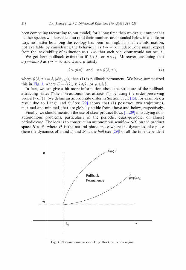
been competing (according to our model) for a long time then we can guarantee thatneither species will have died out (and their numbers are bounded below in a uniformway, no matter how long this ecology has been running). This is new information,not available by considering the behaviour as t-þN: indeed, one might expectfrom the inevitability of extinction as t-N that such behaviour would not occur.We get here pullback extinction if lol1 or mol1: Moreover, assuming that

aðtÞ-a040 as t-�N and l and m satisfy

l4jðmÞ and m4cðl; a0Þ; ð4Þ

where cðl; a0Þ ¼ l1ðdw½l;a0�Þ; then (1) is pullback permanent. We have summarizedthis in Fig. 3, where E ¼ fðl; mÞ: lpl1 or mpl1g:In fact, we can give a bit more information about the structure of the pullback

attracting states (‘‘the non-autonomous attractor’’) by using the order-preservingproperty of (1) (we define an appropriate order in Section 3, cf. [15], for example): aresult due to Langa and Suarez [22] shows that (1) possesses two trajectories,maximal and minimal, that are globally stable from above and below, respectively.Finally, we should mention the use of skew product flows [11,29] in studying non-

autonomous problems, particularly in the periodic, quasi-periodic, or almostperiodic case. The idea is to construct an autonomous semiflow SðtÞ on the productspace H �F; where H is the natural phase space where the dynamics take place(here the dynamics of u and v) and F is the hull (see [29]) of all the time dependent

Pullback Permanence

λ

µ

λ1

λ1

λ=ϕ(µ)

µ=ψ(λ,a0)

Fig. 3. Non-autonomous case. E: pullback extinction region.


terms of the equation. Provided thatF is compact in some appropriate topology thegeneral theory of dissipative dynamical systems can be applied to study SðtÞ on thespace H �F: However, with an entirely general non-autonomous term there is noclear choice of topology on F that will make it compact, a property crucial to thisapproach.3 This is highlighted in the theory of attractors for non-autonomousequations developed by Chepyzhov and Vishik [6,7], while their strongest resultsrequire almost periodicity, precisely in order to obtain a compact F; they studygeneral non-autonomous terms without appealing to skew product flows using theconcepts of a ‘‘kernel’’ and ‘‘kernel sections’’, the latter corresponding exactly to thetime slices AðtÞ of the non-autonomous attractor whose definition we recall below.An outline of this paper is as follows: in Section 2 we introduce the concept of a

process, give the definition of a non-autonomous attractor and state conditions thatguarantee its existence. In Section 3 we study properties of order-preservingprocesses and in particular recall a result about their stability. In Section 4 we studyin detail a non-autonomous logistic equation which governs the behaviour of one ofthe species in absence of the other: this section plays a crucial role throughout all thatfollows. In Section 5 we analyse both the forwards and pullback behaviour of system(1), and finish in Section 6 with the existence of a non-autonomous attractor for (1)and conditions for pullback permanence.

2. Non-autonomous attractors

In this section we introduce the definitions of a non-autonomous attractor and ofpullback permanence.Let ðX ; dÞ be a complete metric space (with metric dÞ and fSðt; sÞgtXs; t; sAR be a

family of mappings satisfying:

(a) Sðt; sÞSðs; tÞu ¼ Sðt; tÞu; for all tpspt; uAX ;(b) Sðt; tÞu is continuous in t; t and u:(c) Sðt; tÞ is the identity in X for all tAR:

Such a map is called a process. Usually, Sðt; tÞu will arise as the value of the solutionof a non-autonomous equation at time t with ‘‘initial condition’’ u at time t: Asremarked in the introduction, for an autonomous equation the solutions onlydepend on t � t; and we can write Sðt; tÞ ¼ Sðt � t; 0Þ:Let D be a non-empty set of parameterized families of non-empty bounded sets

fDðtÞgtAR: In particular, DðtÞ BAD; where BCX is a bounded set. In what

follows, we will consider a fixed base of attraction D and throughout our analysis theconcepts of absorption and attraction will be referred to this fixed base.

3Using uniform convergence on R requires almost periodicity. An interesting extension should be

possible under the assumption that the non-autonomous terms enjoy a uniform modulus of continuity

over R; for then the topology of uniform convergence on compact subsets of R will makeF compact, cf.

[17], and the recent monograph by Chepyzhov and Vishik [8].


For A;BCX define the Hausdorff semidistances as

distðA;BÞ ¼ supaAA

infbAB

dða; bÞ; DistðA;BÞ ¼ infaAA

infbAB

dða; bÞ:

Definition 1.

(a) Given t0AR; we say that Kðt0ÞCX is attracting at time t0 if for every fDðtÞgAD

limt-�N

distðSðt0; tÞDðtÞ;Kðt0ÞÞ ¼ 0:

A family fKðtÞgtAR is attracting if Kðt0Þ is attracting at time t0; for all t0AR:(b) Given t0AR; we say that Bðt0ÞCX is absorbing at time t0 if for every fDðtÞgAD

there exists T ¼ Tðt;DÞAR such that

Sðt0; tÞDðtÞCBðt0Þ for all tpT :

A family fBðtÞgtAR is absorbing if Bðt0Þ is absorbing at time t0; for all t0AR:

Note that every absorbing set at time t0 is attracting.As discussed in the introduction, this notion takes the final time as fixed

and moves the initial time backwards towards �N: We are not evolving onetrajectory backwards in time, but rather we consider the current state of the system(at the fixed time t0) which would result from the same initial condition starting atearlier and earlier times. This is called pullback attraction in the literature (cf.[18,19,30]).

Definition 2. Let fBðtÞgtAR be a family of subsets of X : This family is said to beinvariant with respect to the process S if

Sðt; tÞBðtÞ ¼ BðtÞ for all ðt; tÞAR2; tpt:

Note that this property is a generalization of the classical property of an invariantset for a semigroup. However, in this case we have to define the invariance withrespect to a family of sets depending on a parameter.

Definition 3. The family of compact sets fAðtÞgtAR is said to be the global

non-autonomous (or pullback) attractor associated to the process S if it isinvariant, attracts every fDðtÞgAD (for all t0AR) and minimal in the sensethat if fCðtÞgtAR is another family of closed attracting sets, then AðtÞCCðtÞ forall tAR:

The general result on the existence of non-autonomous attractors is a general-ization of the abstract theory for autonomous dynamical systems [11,32]:


Theorem 4 (Crauel et al. [10], Schmalfuss [30]). Assume that there exists a family of

compact absorbing sets. Then, the family fAðtÞgtAR defined by

AðtÞ ¼[

DAD

LðD; tÞ

is the global non-autonomous attractor, where LðD; tÞ is the omega-limit set at time t of

D fDðtÞgAD;

LðD; t0Þ ¼\

spt0

[tps

Sðt0; tÞDðtÞ:

Using the pullback idea introduced above we can now give the followingdefinition of ‘‘pullback permanence’’. As in [5] we suppose that X ¼ X0,@X0; whereX0 is open, and X0; @X0 are invariant with respect to the process S: In ourapplication, @X0 will be the set of solutions with at least one component identicallyzero.

Definition 5. We say that a system has the property of pullback permanence (or thatit is permanent in the pullback sense) if there exists a time-dependent family ofbounded sets U :R/X ; satisfying

(a) UðtÞ absorbs every bounded set DCX (cf. Definition 1).(b) DistðUðtÞ; @X0Þ40 for all tAR:

Following Definition 3, we can define a global attractor AþCX0 that attractsevery bounded set in X0: its existence follows using Theorem 4.

3. Order-preserving non-autonomous differential equations

In this section we define what it means for a process to be order-preserving. Forsuch a process we can determine some of the structure of the non-autonomousattractor and prove the existence of a minimal and maximal trajectory on theattractor with some particular stability properties.

Definition 6. We say that the process fSðt; sÞ :X-XgtXs is order-preserving if there

exists an order relation ‘%’ in X such that, if w1%w2; then Sðt; sÞw1%Sðt; sÞw2 forall tXs:

The next definition generalizes the concept of equilibria in [14] (see also [1]in the stochastic case and [9] in the non-autonomous case under strongerconditions).


Definition 7. Let S be an order-preserving process. We call the continuous mapw :R-X a complete trajectory if, for all sAR; we have

Sðt; sÞwðsÞ ¼ wðtÞ for tXs:

From ð%w; %wÞ such that

%wðtÞ% %wðtÞ; for all tAR; we can define the ‘‘interval’’

I %w

%w ðtÞ ¼ fwAX :

%wðtÞ%w% %wðtÞg:

The following result was proved in [22] and it gives sufficient conditions for theexistence of upper and lower asymptotically stable complete trajectories, andprovides some information about the structure of the non-autonomous attractor.

Theorem 8. Let S be an order-preserving process and AðtÞ its associated pullback

attractor attracting time-dependent families of sets in a base of attraction D: Let

%w; %wAD be such that

%wðtÞ% %wðtÞ; for all tAR; and assume that

AðtÞCI %w

%w ðtÞ 8tAR:

Then there exist two trajectories w*ðtÞ; wnðtÞAAðtÞ such that

(i) w*ðtÞ%w%wnðtÞ; 8tAR and 8wAAðtÞ:

(ii) w*ðwnÞ is minimal (maximal) in the sense that there is no complete trajectory in

the interval Iw*

%w ðI %w

wnÞ:(iii) w

*ðtÞ is globally asymptotically stable from below, that is, for all zAD with

%wðtÞ%zðtÞ%w

*ðtÞ; for all tAR; we have

lims-�N

dðSðt; sÞzðsÞ;w*ðtÞÞ ¼ 0:

wnðtÞ is globally asymptotically stable from above, that is, for all zAD with

wnðtÞ%zðtÞ% %wðtÞ; for all tAR; we have

lims-�N

dðSðt; sÞzðsÞ;wnðtÞÞ ¼ 0:

4. The non-autonomous logistic equation

In the absence of one species, the evolution of the other is given by the non-autonomous logistic equation

wt � Dw ¼ qðx; tÞw � bðtÞw2 in O� ðs;þNÞ;w ¼ 0 on @O� ðs;þNÞ;wðx; sÞ ¼ w0ðxÞ in O;

8><>: ð5Þ

where qALNðO� ðs;NÞÞ and 0obðtÞpB for all tAR:


Firstly, we introduce some results which will be very useful. Given fALNðOÞ wedenote by l1ðf Þ the principal eigenvalue of the problem

�Dw þ f ðxÞw ¼ sw in O;

w ¼ 0 on @O;

(ð6Þ

and by j1ðf Þ the unique positive eigenfunction such that jjj1ðf ÞjjN ¼ 1: It is wellknown that l1ðf Þ is increasing and continuous in f ; decreasing and continuous in Oand that if f ðxÞ40 in O then (see [23, Theorem 6.4])

limb-N

l1ðbf Þ ¼ N: ð7Þ

We denote l1 :¼ l1ð0Þ: Finally, given fALNðOÞ and eAR; e40; we consider the non-linear elliptic equation

�Dw ¼ f ðxÞw � ew2 in O;

w ¼ 0 on @O:

(ð8Þ

The next result collects the main results on the existence and uniqueness of a positivesolution for (8) and some important properties of this solution.

Lemma 9. Problem (8) possesses a positive solution if, and only if, l1ð�f Þo0:Furthermore, if such a solution exists then it is unique: we denote it by w½f ;e� and set

w½f ;e� 0 if l1ð�f ÞX0: In addition,

(a) w½f ;e� is bounded below:

� l1ð�f Þe

j1ð�f Þpw½f ;e� in O; and ð9Þ

(b) the maps fALNðOÞ/w½f ;e� and eAð0;NÞ/w½f ;e� are continuous.

Proof. The existence and uniqueness of a positive solution are well known, see forinstance [14]. Observe that the pair

ð%w; %wÞ ¼ � l1ð�f Þ

ej1ð�f Þ; fM

e

�

is a sub-supersolution of (8), where fM :¼ ess supxAO f ðxÞ: Indeed, it is not hard toprove that

%w and %w satisfy the following inequalities:

�D%wpf ðxÞ

%w � e

%w2; �D %wXf ðxÞ %w � e %w

2 in O


and

%w ¼ � l1ð�f Þ

ej1ð�f Þp� l1ð�fMÞ

e¼ fM � l1

eo

fM

e¼ %w:

Thus,

� l1ð�f Þe

j1ð�f Þpw½f ;e�pfM

eð10Þ

from which (9) follows. Now, by (10), the continuity of the maps f/w½f ;e� and

e/w½f ;e� can be obtained. &

The following result provides us with the existence and uniqueness of positivesolution for (5), as well as its ‘‘forward’’ and ‘‘pullback’’ asymptotic behaviour. Weconsider the Banach space

C0ð %OÞ :¼ fuACð %OÞ: u ¼ 0 on @Og

ordered by its positive cone P :¼ fuAC0ð %OÞ: uX0 in Og:

Proposition 10. Given w0APWf0g; there exists a unique positive solution of (5),denoted by y½q;b�ðt; s;w0Þ; which is strictly positive for t4s: Moreover:

(a) y½q;b�ðt; s;w0Þ is increasing in q and decreasing in b.

Now, assume that qðx; tÞ qðxÞ: Then,

(b) If bðtÞ ¼ b040; then jjy½q;b0�ðt; s;w0Þ � w½q;b0�jjN-0 as t-N or s-�N:

(c) If l1ð�qÞ40; then jjy½q;b�ðt; s;w0ÞjjN-0 as t-N or s-�N:

(d) If l1ð�qÞo0 and bðtÞ-0 when t-N; then jjy½q;b�ðt; s;w0ÞjjN-N as t-N:

(e) Given tAR and l1ð�qÞo0; there exist VACð %OÞ; V40; and Tðt;w0Þ such that

VðxÞpy½q;b�ðt; s;w0ÞprðtÞ for any spTðt;w0Þ; ð11Þ

where

rðtÞ ¼ ejjqjjNt

12

R t

�NejjqjjNtbðtÞ dt

:

Proof. The existence and uniqueness follow in a standard way. The positivity of thesolution for t4s follows by the strong maximum principle for parabolic equations.For part (a), take q1ðx; tÞpq2ðx; tÞ for all xAO; tXs: Then, y½q1;b�ðt; s;w0Þ is a

subsolution of (5) with q ¼ q2; and so by the uniqueness of the solution it follows


that

y½q1;b�ðt; s;w0Þpy½q2;b�ðt; s;w0Þ:

A similar reasoning shows the monotony with respect to b:Part (b) has been proved, for instance, in [4, Lemma 5.1] when t-N: As we have

indicated before in the autonomous case

y½q;b0�ðt; s;w0Þ ¼ y½q;b0�ðt � s; 0;w0Þ;

and so the result follows when s-�N:For part (c), since l1ð�qÞ40 and by the continuity of the principal eigenvalue

with respect to the domain, there exists a regular domain O1 such that OC %OCO1and

0olO11 ð�qÞol1ð�qÞ;

where lO11 ð�qÞ stands for the principal eigenvalue of (6) in O1 with f ¼ �q: We

denote by jO11 ð�qÞ its associated positive eigenfunction and take %w :¼

Kegðt�sÞjO11 ð�qÞ: Then, %w is a supersolution of (5) provided that

KjO11 ð�qÞXw0 in O;

gþ lO11 ð�qÞ þ KbðtÞegðt�sÞjO11 ð�qÞX0 in O� ðs;NÞ:

We can take K sufficiently large and �lO11 ð�qÞpgo0; and so

y½q;b�ðt; s;w0ÞpKegðt�sÞjO11 ð�qÞ

whence the result is obtained.We now prove (d). Fix M40 and l1ð�qÞo0: Taking

e :¼ � l1ð�qÞ2M

;

since bðtÞ-0 as t-N; there exists teAR such that for any tXte

bðtÞpe:

Observe that,

y½q;b�ðt; s;w0Þ ¼ y½q;b�ðt; te; ze;sÞ; ð12Þ

where

ze;s ¼ y½q;b�ðte; s;w0Þ:


Now, by part (a) we have that

y½q;b�ðt; te; ze;sÞXy½q;e�ðt; te; ze;sÞ for tXte: ð13Þ

By part (b), there exists t1AR such that for tXt1; we get

y½q;e�ðt; te; ze;sÞXw½q;e� þl1ð�qÞ2e

X� l1ð�qÞe

j1ð�qÞ þ l1ð�qÞ2e

;

this last inequality thanks to (9). Therefore, by (12) and (13), for tXt1 we get

y½q;b�ðt; s;w0ÞX� l1ð�qÞe

j1ð�qÞ þ l1ð�qÞ2e

;

and so, since jjj1ð�qÞjjN

¼ 1; we obtain

jjy½q;b�ðt; s;w0ÞjjNXM:

This completes part (d).For part (e), since bðtÞpB for all tAR; it follows that

y½q;B�ðt � s; 0;w0Þ ¼ y½q;B�ðt; s;w0Þpy½q;b�ðt; s;w0Þ

and the existence of a positive function V follows by part (b). On the other hand,

%w :¼ yðt; s; jjw0jjNÞ

is a supersolution of (5), where yðt; s; y0Þ is the solution of

y0 ¼ jjqjjN

y � bðtÞy2; yðsÞ ¼ y0

which is given explicitly by

yðt; s; y0Þ ¼ejjqjjNðt�sÞ

1y0þR t

sejjqjjNðr�sÞbðrÞ dr

:

Now, it suffices to let s-�N: This completes the proof. &

Proposition 10 provides us with a complete description of the long-time behaviourof the positive solution of (5). In the autonomous case, part (b), w½q;b0� is globally

asymptotically stable, and so the species is driven to extinction when l1ð�qÞX0 and(5) is permanent when l1ð�qÞo0:In the non-autonomous case, the species is driven to extinction in the ‘‘forward’’

and ‘‘pullback’’ senses when l1ð�qÞ40: However, when l1ð�qÞo0 there is a drasticchange of behaviour: by part (d), we cannot expect forward permanence, whereas in[22] it was proved that for l1ð�qÞo0 Eq. (5) is permanent in the pullback sense.


5. Non-autonomous Lotka–Volterra competition model

Our first result in this section guarantees the existence and uniqueness of a positivesolution of (1) and provides some helpful estimates.

Theorem 11. Given u0; v0APWf0g; there exists a unique positive solution of

(1), denoted by ðuðt; s; u0; v0Þ; vðt; s; u0; v0ÞÞ; which is strictly positive for t4s:Moreover,

y½l�by½m;c�;a�pupy½l;a� y½m�dy½l;a�;c�pvpy½m;c�: ð14Þ

Proof. We take

ð%u; %uÞ :¼ ðy½l�by½m;c�;a�; y½l;a�Þ ð

%v; %vÞ :¼ ðy½m�dy½l;a�;c�; y½m;c�Þ:

Firstly, by Proposition 10(a), it is clear that%up %u and

%vp%v: Moreover, it is not hard

to prove that this couple satisfies

%ut � D

%u ¼

%uðl� aðtÞ

%u � b%vÞ; %ut � D %u ¼ %uðl� aðtÞ %uÞX %uðl� aðtÞ %u � b

%vÞ;

%vt � D

%v ¼

%vðm� c

%v � d %uÞ; %vt � D%v ¼ %vðm� c%vÞX%vðm� c%v � d

%uÞ:

Thus the existence of a positive solution of (1) follows from Theorem 8.3.2 in [31].Uniqueness follows by a standard argument to complete the proof. &

5.1. Asymptotic behaviour forward in time

The asymptotic behaviour of (1) depends on the values of l and m: The next resultshows cases where the trivial solution and the semi-trivial one are globallyasymptotically stable, and so at least one species is driven to extinction.

Proposition 12. Suppose lol1:

(a) If mpl1; then ðuðt; s; u0; v0Þ; vðt; s; u0; v0ÞÞ-ð0; 0Þ as t-N:(b) If m4l1; then ðuðt; s; u0; v0Þ; vðt; s; u0; v0ÞÞ-ð0;w½m;c�Þ as t-N:

Proof. If lol1; then observe that l1ð�lÞ ¼ l1 � l40: Hence, from (14) andProposition 10(c) we get that uðt; s; u0; v0Þ-0 as t-N: Similarly, when mpl1 we getthat vðt; s; u0; v0Þ-0 as t-N:Now, we assume m4l1: Let d40 be such that m4l1 þ dd: For such d there exists

t0AR such that

jjuðt; s; u0; v0ÞjjNod for any tXt0:


On the other hand, using the definition of y½q;b� we obtain

u ¼ y½l�bv;a� and v ¼ y½m�du;c�: ð15Þ

Then, by (14) and Proposition 10(a), we have

y½m�dd;c�py½m�du;c� ¼ vpy½m;c� for tXt0:

It is sufficient to apply Proposition 10(b) and the continuity of the mapf/w½f ;e�: &

The following result shows that the system is not permanent when l and m satisfyan easily verifiable condition. The system is not permanent because one species (u)increases indefinitely and drives the other to extinction.We note here that although under the condition aðtÞ-0 the equation is

‘‘asymptotically autonomous’’ in the sense of Markus [26] (see also more recentworks by Thieme [33], Mischaikow et al. [27]) the general results that are availablefor such systems are not sufficiently detailed to give us all the information weneed: for example, it is known that if all the solutions of the limit equation areunbounded then so are the solutions of the non-autonomous equation [26], but wewish to show that while one species grows without bound the other is driven toextinction.

Proposition 13. Suppose aðtÞ-0 as t-N: If l4l1ðbw½m;c�Þ; then

ðuðt; s; u0; v0Þ; vðt; s; u0; v0ÞÞ-ðN; 0Þ as t-N:

Observe that w½m;c� ¼ 0 if mpl1; so l4l1ðbw½m;c�Þ means l4l1 when mpl1:

Proof. Assume mpl1; then by Proposition 10(c) we have that vpy½m;c�-0 as t-N:

Moreover, since l4l1; we can obtain that

l� by½m;c�4l1 for tXt1:

Hence,

l1ð�lþ by½m;c�Þol1ð�l1Þ ¼ 0;

and so, by Proposition 10(d)

y½l�by½m;c�;a�-N;

and the result follows by (14).


Now, suppose m4l1 and l4l1ðbw½m;c�Þ: We define

e :¼l� l1ðbw½m;c�Þ

2b:

Since vpy½m;c�-w½m;c� as t-N; then there exists te such that for tXte

vpw½m;c� þ e;

and so, by (15)

u ¼ y½l�bv;a�Xy½l�bðw½m;c�þeÞ;a� for tXte:

Since, aðtÞ-0 as t-N; given dAð0; 1� there exists td such that for tXtd we haveaðtÞpd; and so,

uXy½l�bðw½m;c�þeÞ;a�Xy½l�bðw½m;c�þeÞ;d�; tXmaxfte; tdg: ð16Þ

Now, observe that

l1ð�lþ bw½m;c� þ beÞ ¼ l1ðbw½m;c�Þ � lþ be ¼ �l� l1ðbw½m;c�Þ

2o0: ð17Þ

Taking account (16) and (17), a similar argument to the used in the proof ofProposition 10(d) shows that given a small positive s40 there exists ts such that fortXts; we have

uXF :¼l� l1ðbw½m;c�Þ

2dj1ð�lþ bðw½m;c� þ eÞÞ � s: ð18Þ

Taking s such that

0osol� l1ðbw½m;c�Þ

4pl� l1ðbw½m;c�Þ

4d; ð19Þ

we get that

jjujjNXjjFjj

NXl� l1ðbw½m;c�Þ

4d:

Hence, it is sufficient to take d sufficiently small in order to show that u approachesinfinity.Finally, observe that by (18) we get

v ¼ y½m�du;c�py½m�dF;c�; tXts;


and if we can take mol1ðdFÞ; by Proposition 10(b) we obtain that v goes to 0: But,mol1ðdFÞ is equivalent to

mol1l� l1ðbw½m;c�Þ

2dj1ð�lþ bðw½m;c� þ eÞÞ

� � s;

which is true by (19) and (7) taking d sufficiently small. This completes theproof. &

5.2. Pullback asymptotic behaviour

The next two results show ‘‘pullback’’ extinction for some values of l and m: Thefirst one is similar to Proposition 12 and so we omit the proof.

Proposition 14. Suppose lol1:

(a) If mpl1; then ðuðt; s; u0; v0Þ; vðt; s; u0; v0ÞÞ-ð0; 0Þ as s-�N:(b) If m4l1; then ðuðt; s; u0; v0Þ; vðt; s; u0; v0ÞÞ-ð0;w½m;c�Þ as s-�N:

Hereafter, we denote A :DðAÞ/C0ð %OÞ the linear operator associated to theLaplacian.

Proposition 15. Given tAR; l4l1 and mpl1; then

ðuðt; s; u0; v0Þ; vðt; s; u0; v0ÞÞ-ðy½l;a�ðt; s; u0Þ; 0Þ as s-�N:

Proof. Since mpl1; then vpy½m;c�-0 as s-�N: Now, given d40 there exists sdsuch that

vðt; s; u0; v0Þpd for spsd:

Hence, by (15), we get

y½l�bd;a�py½l�bv;a� ¼ upy½l;a� for spsd;

and so,

y½l�bd;a� � y½l;a�pu � y½l;a�p0 for spsd:

Thus, it suffices to prove that

wd :¼ y½l�bd;a� � y½l;a�-0; as d-0: ð20Þ


It is not hard to prove that wd satisfies

ðwdÞt � Dwd ¼ lwd � bdy½l�bd;a� � aðtÞwdðy½l�bd;a� þ y½l;a�Þ:

Now, if we denote by

gdðr; sÞ ¼ l� aðrÞðy½l�bd;a�ðr; s; u0Þ þ y½l;a�ðr; s; u0ÞÞ

and writing wd from the variation of constants formula, we obtain

wdðt; s; u0Þ ¼Z t

s

e�Aðt�rÞðgdðr; sÞwdðr; s; u0Þ � bdy½l�bd;a�ðr; s; u0ÞÞ dr;

and so, since jje�Aðt�rÞjjopp1; we get

jjwdðt; s; u0ÞjjNpZ t

s

jjgdðr; sÞjjNjjwdðr; s; u0ÞjjN dr þ bd

Z t

s

jjy½l�bd;a�ðr; s; u0ÞjjN dr;

and by Gronwall’s lemma we obtain

jjwdðt; s; u0ÞjjNpbdZ t

s

jjy½l�bd;a�ðr; s; u0ÞjjN dre

R t

sjjgdðr;sÞjjN dr

: ð21Þ

On the other hand, by Proposition 10 we have

jjy½l�bd;a�ðt; s; u0ÞjjNpjjy½l;a�ðt; s; u0ÞjjNprðtÞ for spTðtÞ;

for some TðtÞ and rðtÞ independent of d: Now, (20) follows by taking d to zero in(21). &

The next result shows that for a fixed final time t0; the positive solution of (1) isbounded away by positive functions for s sufficiently small.

Proposition 16. Fix t0AR: Assume that

infsAð�N;t0�

aðsÞ ¼ aðt0Þ40;

l4l1ðbw½m;c�Þ; and m4l1ðdw½l;aðt0Þ�Þ:

Then, there exist s0pt0 and eiAC0ð %OÞ positive functions (depending on t0), such that

for all sps0:

uðt0; s; u0; v0ÞXe1 and vðt0; s; u0; v0ÞXe2:


Proof. Since aðt0ÞpaðtÞpA for all tpt0; we have

y½l;A�ðt0; s; u0Þpy½l;a�ðt0; s; u0Þpy½l;aðt0Þ�ðt0; s; u0Þ for spt0:

Since l4l1ðbw½m;c�Þ; m4l1ðdw½l;aðt0Þ�Þ; we can choose e40 sufficiently small such that

l4l1ðbðw½m;c� þ eÞÞ and m4l1ðdðw½l;aðt0Þ� þ eÞÞ: ð22Þ

For such e40; and by Proposition 10(b), we obtain

w½l;A� � epy½l;a�ðt0; s; u0Þpw½l;aðt0Þ� þ e for sps0;

for some s0: Using again Proposition 10(a) and (14), we get

y½m�dðw½l;aðt0Þ�þeÞ;c�pv for sps0: ð23Þ

On the other hand, by Proposition 10(a)

y½l�by½m;c�;A�py½l�by½m;c�;a�pu

and by part (b),

w½m;c� � epy½m;c�ðt0; s; u0Þpw½m;c� þ e for sps0;

and so,

y½l�bðw½m;c�þeÞ;A�pu: ð24Þ

Now, by Proposition 10(b), we have that as s-�N;

y½m�dðw½l;aðt0Þ�þeÞ;c� -w½m�dðw½l;aðt0Þ�þeÞ;c�;

y½l�bðw½m;c�þeÞ;A� -w½l�bðw½m;c�þeÞ;A�:

Proposition 10(b), (22)–(24) complete the proof. &

Assuming that aðtÞ tends to a positive constant as t-�N; we obtain asimilar result to Proposition 16 but where the conditions on l and m do notdepend on t:


Corollary 17. Assume aðtÞ-a040 as t-�N; for each tAR

infsAð�N;t�

aðsÞ ¼ aðtÞ40;

l4l1ðbw½m;c�Þ and m4l1ðdw½l;a0�Þ:

Then, for all tAR; there exist s0ðtÞpt and fiAC0ð %OÞ positive functions (depending on t),such that for all sps0 it holds:

uðt; s; u0; v0ÞXf1 and vðt; s; u0; v0ÞXf2:

Proof. Since m4l1ðdw½l;a0�Þ and from the continuity of the map e/w½l;e�; there exists

e40 such that m4l1ðdw½l;a0�e�Þ: On the other hand, since aðtÞ-a0 as t-�N; there

exists TAR such that for all tpT ; a0 � epaðtÞpaðtÞpA: Then, for any t0pT wehave that

m4l1ðdw½l;aðt0Þ�Þ;

and so by Proposition 16, we get that there exist two positive functions ei such that

uðt0; s; u0; v0ÞXe1 and vðt0; s; u0; v0ÞXe2:

Furthermore, for all tXt0 we have

uðt; s; u0; v0Þ ¼ uðt; t0; uðt0; s; u0; v0Þ; vðt0; s; u0; v0ÞÞ

from which, by the strong maximum principle, we obtain the result. &

6. Existence of a non-autonomous attractor and pullback permanence for the Lotka–

Volterra competition model

We define X :¼ C0ð %OÞ � C0ð %OÞ and the following process in X : for t; sAR; tXs;

Sðt; sÞ :X/X ; Sðt; sÞðu0; v0Þ ¼ ðuðt; s; u0; v0Þ; vðt; s; u0; v0ÞÞ;

where ðuðt; s; u0; v0Þ; vðt; s; u0; v0ÞÞ is the unique positive solution of (1) for u0; v0AP:Moreover, in X we define the following order: given ðu1; v1Þ; ðu2; v2ÞAX ;

ðu1; v1Þ%ðu2; v2Þ if ; and only if ; u1pu2 and v1Xv2;

where ‘‘p’’ is the order defined by P in C0ð %OÞ: It is well known, see [15], that Sðt; sÞ isan order-preserving process, that is, if ðu1; v1Þ$ðu2; v2Þ; thenSðt; sÞðu1; v1Þ%Sðt; sÞðu2; v2Þ: Moreover, we consider the norm jðu; vÞj

N¼ jjujj

Nþ

jjvjjNin X :

In the next two sections we will prove the existence of a non-autonomous attractorfor (1).


6.1. Absorbing set in X

Let DCX be bounded, i.e., supdAD jdjNpM; for M40; and ðu0; v0ÞAD: By (14)

and Proposition 10(e), there exists Tðt; u0; v0ÞAR such that

jjuðt; s; u0; v0ÞjjNpjjy½l;a�ðt; s; u0ÞjjNprlðtÞ for spTðtÞ; ð25Þ

where

rlðtÞ ¼2eltR t

�NeltaðtÞ dt

:

Similarly,

jjvðt; s; u0; v0ÞjjNprmðtÞ for spTðtÞ; ð26Þ

where

rmðtÞ ¼2emt

cR t

�Nemt dt

¼ 2mc:

Clearly, this means that the ball in X with radius r1ðtÞ ¼ rlðtÞ þ rmðtÞ; BX ð0; r1ðtÞÞ; isabsorbing for the process Sðt; sÞ:

6.2. Absorbing set in C10ð %OÞ � C10ð %OÞ

In order to obtain a family of absorbing sets in C10ð %OÞ we need the following resultfrom [28], see also [4, Lemma 3.1]. Here, for a Banach space Y ; Y b will denote the

usual fractional power spaces with norm j � jb: Recall that A :DðAÞ/C0ð %OÞ is thelinear operator associated to the Laplacian.

Lemma 18. The operator A generates an analytic semigroup on Y ¼ Ck0 ð %OÞ for k ¼

0; 1: Moreover,

Y b+Ckþq0 ð %OÞ for q ¼ 0; 1 and 2b4q:

Given DCX bounded, we define for rXs

hðr; sÞ ¼ luðr; s; u0; v0Þ � aðrÞu2ðr; s; u0; v0Þ � buðr; s; u0; v0Þvðr; s; u0; v0Þ:

Then, writing u from the variation of constants formula, we obtain

uðt; s; u0; v0Þ ¼ e�Aðt�sÞu0 þZ t

s

e�Aðt�rÞhðr; sÞ dr:

Hence, between t � 1 and t; we get

uðt; s; u0; v0Þ ¼ e�Auðt � 1; s; u0; v0Þ þZ t

t�1e�Aðt�rÞhðr; sÞ dr:


Hence,

juðt; s; u0; v0Þjb ¼ jjAbuðt; s; u0; v0ÞjjNpjjAbe�Ajjopjjuðt � 1; s; u0; v0ÞjjN

þ suprA½t�1;t�

jjhðr; sÞjjN

Z t

t�1jjAbe�Aðt�rÞjjop dr:

Now, using the estimate

jjAbe�Aðt�rÞjjoppCbðt � rÞ�be�dðt�rÞ

for some constants Cb; d40 (cf. Henry [13]), and estimates (25) and (26), we obtainthe existence of MðtÞ and T0ðtÞ such that

juðt; s; u0; v0ÞjbpMðtÞ for all spT0ðtÞ;

with bo1� e; and any eAð0; 1Þ: Applying now Lemma 18 with q ¼ 1 and b41=2;we obtain

jjuðt; s; u0; v0ÞjjC1pR1ðD; tÞ for all spT0ðtÞ:

Similarly, it can be proven that

jjvðt; s; u0; v0ÞjjC1pR2ðD; tÞ for all spT0ðtÞ;

for some R2ðD; tÞ; and so the ball in C10ð %OÞ � C10ð %OÞ; Bð0;RðtÞÞ is absorbing inC10ð %OÞ � C10ð %OÞ; for RðtÞ ¼ R1ðtÞ þ R2ðtÞ; where again we have used the normjðu; vÞjC1ð %OÞ ¼ jjujjC1ð %OÞ þ jjvjjC1ð %OÞ in C10ð %OÞ � C10ð %OÞ:We can repeat the argument taking Y ¼ C10ð %OÞ and D a bounded set in Y � Y : In

this case, using Lemma 18 again, we obtain

jjuðt; s; u0; v0ÞjjC2pNðD; tÞ for all spT1ðtÞ;

and hence, the existence of an absorbing set that is bounded in C20ð %OÞ � C20ð %OÞ; andso compact in X :Analogously, we can show the existence of the global attractor Aþ attracting

every bounded set in X0:

6.3. On the structure of the pullback attractor and pullback permanence

In this section we apply the results of Section 3 to our model. We take

%wðtÞ ¼ ð0; rmðtÞÞ and %wðtÞ ¼ ðrlðtÞ; 0Þ:

Firstly, observe that%wðtÞ% %wðtÞ: On the other hand, by (25) and (26) it follows that

AðtÞCI %w

%w ðtÞ:


Finally, we define the base of attraction in our model as

D :¼ w :R/X continuous; such that; lims-�N

egs

jjwðsÞjjN

¼ 0�

;

where g ¼ minfl; mg: Note, that given w ¼ ðu; vÞAD;

lims-�N

distðSðt; sÞðuðsÞ; vðsÞÞ;AðtÞÞ ¼ 0: ð27Þ

Indeed, we have that for s small enough

jjuðt; s; uðsÞ; vðsÞÞjjNpjjy½l;a�ðt; s; uðsÞÞjj

Np

elt

els

jjuðsÞjjN

þR t

seltaðtÞ dt

prlðtÞ:

Moreover, it is clear that ð%w; %wÞAD: So, applying Theorem 8, there exist complete

trajectories w*(minimal) and wn (maximal) that are stable in the sense of Theorem 8.

In a similar way, for Aþ we can also apply Theorem 8 for

%wðtÞ ¼ ðf1ðtÞ; rmðtÞÞ; %wðtÞ ¼ ðrlðtÞ; f2ðtÞÞ;

so that, for strictly positive initial data, the non-autonomous attractor is boundedabove and below by strictly positive bounds. Finally, we can conclude the pullbackpermanence of our model.

Theorem 19. Assume that aðtÞ-a040 as t-�N; for each tAR

infsAð�N;t�

aðsÞ ¼ aðtÞ40;

l4l1ðbw½m;c�Þ and m4l1ðdw½l;a0�Þ:

Then (1) is permanent in the pullback sense.

Proof. We write X ¼ X0,@X0; where X0 ¼ ðintPÞ2 and @X0 ¼ XWX0: Thepermanence follows with

UðtÞ ¼ fwAX : ðf1ðtÞ; rmðtÞÞ%w%ðrlðtÞ; f2ðtÞÞg;

where f1; f2 are defined in Corollary 17 and rl and rm in (25) and (26), respectively. By

Section 6.1, UðtÞ is absorbing and by Corollary 17 DistðUðtÞ; @X0Þ40: Thiscompletes the proof. &


7. Conclusions

We have considered a Lotka–Volterra system with a non-autonomous term thatproduces only a weak dissipativity effect. This effect is so weak that there are nobounded absorbing sets, and hence we cannot expect any kind of permanence ast-N: In order to understand the dynamics of the system further we haveintroduced the concept of ‘‘pullback permanence’’: for our example we could showthe existence of a time dependent family of sets, bounded above and below bypositive functions, that absorbs every trajectory of the system ‘‘in the pullbacksense’’. This gives a sense in which, even though one species will eventually die out,the system exhibits some kind of permanence: at any time t0; no matter how long thesystem has been running, the species numbers are uniformly bounded below.We note here that the region in the ðl; mÞ-plane defined by l4l1ðbw½m;c�Þ and

m4l1ðdw½l;a0�Þ can be empty depending on the values of the parameters a0; b; c and d

(cf. [24, Section 7]). Even in the autonomous case, aðtÞ ¼ a40; results of permanenceare not known when bc is large with respect to ad: In this case the region defined byl4l1ðbw½m;c�Þ and m4l1ðdw½l;a�Þ is empty, and it is known that if l and m belong tothe region defined by lol1ðbw½m;c�Þ and mol1ðdw½l;a�Þ; then there exists an unstablestationary positive solution of (1) (cf. [25, Theorem 5.3]).To understand the behaviour of this model in more detail would require an

analysis of the local stability and instability of the complete trajectories that play amajor role in the dynamics. There is some progress on this for the ODE version of (1)(see [21]), but in general the subject is still in its infancy: even one-dimensional non-autonomous examples show a much richer and more complex dynamics than theircorresponding autonomous counter-parts (cf. [20]).As emphasized above, the notion of ‘‘pullback permanence’’ that we have defined

is not intended as a candidate to replace the standard definition. Rather we believethat the results presented here offer strong evidence that the pullback procedure is avaluable tool with which we can further our understanding of non-autonomoussystems.

References

[1] L. Arnold, I. Chueshov, Order-preserving random dynamical systems: equilibria, attractors,

applications, Dyn. Stability Systems 13 (1998) 265–280.

[2] R.S. Cantrell, C. Cosner, Should a park be an island?, SIAM J. Appl. Math. 53 (1993) 219–252.

[3] R.S. Cantrell, C. Cosner, Practical persistence in ecological models via comparison methods, Proc.

Roy. Soc. Edinburgh A 126 (1996) 247–272.

[4] R.S. Cantrell, C. Cosner, V. Hutson, Permanence in ecological systems with spatial heterogeneity,

Proc. Roy. Soc. Edinburgh A 123 (1993) 533–559.

[5] R.S. Cantrell, C. Cosner, V. Hutson, Ecological models, permanence and spatial heterogeneity,

Rocky Mountain J. Math. 26 (1996) 1–35.

[6] V. Chepyzhov, M. Vishik, A hausdorff dimension estimate for kernel sections of non-autonomous

evolution equations, Indiana Univ. Math. J. 42 (3) (1993) 1057–1076.

[7] V.V. Chepyzhov, M.I. Vishik, Attractors of non-autonomous dynamical systems and their

dimension, J. Math. Pures Appl. 73 (1994) 279–333.


[8] V.V. Chepyzhov, M.I. Vishik, Attractors for Equations of Mathematical Physics, AMS Colloquium

Publications, Vol. 49, AMS, Providence, RI, 2002.

[9] I. Chueshov, Order-preserving skew-product flows and non-autonomous parabolic systems, Acta

Appl. Math. 65 (2001) 185–205.

[10] H. Crauel, A. Debussche, F. Flandoli, Random attractors, J. Dyn. Differential Equations 9 (1997)

341–397.

[11] J. Hale, Asymptotic Behavior of Dissipative Systems, Mathematical Surveys and Monographs, AMS,

Providence, RI, 1998.

[12] J. Hale, P. Waltman, Persistence in infinite dimensional systems, SIAM J. Math. Anal. 9 (1989)

388–395.

[13] D. Henry, Geometric Theory of Semilinear Parabolic Equations, in: Lecture Notes in Mathematics,

Vol. 840, Springer, Berlin, 1981.

[14] P. Hess, Periodic–Parabolic Boundary Value Problems and Positivity, in: Pitman Research Notes in

Mathematics, Vol. 247, Harlow Longman, New York, 1991.

[15] P. Hess, A.C. Lazer, On an abstract competition model and applications, Nonlinear Anal. 16 (1991)

917–940.

[16] V. Hutson, K. Schmitt, Permanence in dynamical systems, Math. Biosci. 111 (1992) 1–71.

[17] R.A. Johnson, P.E. Kloeden, Nonautonomous attractors of skew product flows with digitized driving

systems, Electronic J. Differential Equations 58 (2001) 16pp.

[18] P.E. Kloeden, B. Schmalfuss, Nonautonomous systems, cocycle attractors and variable time-step

discretization, Numer. Algorithms 14 (1997) 141–152.

[19] P.E. Kloeden, B. Schmalfuss, Asymptotic behaviour of non-autonomous difference inclusions,

Systems Control Lett. 33 (1998) 275–280.

[20] J.A. Langa, J.C. Robinson, A. Suarez, Stability, instability, and bifurcation phenomena in non-

autonomous differential equations, Nonlinearity 15 (2002) 887–903.

[21] J.A. Langa, J.C. Robinson, A. Suarez, Forwards and pullback behaviour of a non-autonomous

Lotka–Volterra system, submitted.

[22] J.A. Langa, A. Suarez, Pullback permanence for non-autonomous partial differential equations,

Electron. J. Differential Equations 72 (2002).

[23] J. Lopez-Gomez, The maximum principle and the existence of principal eigenvalues for some linear

weighted boundary value problems, J. Differential Equations 127 (1996) 263–294 doi:10.1006/

jdeq.1996.0070.

[24] J. Lopez-Gomez, On the structure of the permanence region for competing species models with

general diffusivities and transport effects, Discrete Continuous Dyn. Systems 2 (1996) 525–542.

[25] J. Lopez-Gomez, J.C. Sabina de Lis, Coexistence states and global attractivity for some convective

diffusive competing species models, Trans. Amer. Math. Soc. 347 (1995) 3797–3833.

[26] L. Markus, Asymptotically autonomous differential systems, in: S. Lefschetz (Ed.), Contributions to

the Theory of Nonlinear Oscillations III, Annals of Mathematics Studies, Vol. 36, Princeton

University Press, Princeton, NJ, 1956, pp. 17–29.

[27] K. Mischaikow, H.L. Smith, H.R. Thieme, Asymptotically autonomous semiflows: chain recurrence

and Liapunov functions, Trans. Amer. Math. Soc. 347 (1995) 1669–1685.

[28] X. Mora, Semilinear parabolic problems define semiflows on Ck spaces, Trans. Amer. Math. Soc. 278

(1983) 21–55.

[29] G. Sell, Non-autonomous differential equations and dynamical systems, Trans. Amer. Math. Soc. 127

(1967) 241–283.

[30] B. Schmalfuss, Attractors for the non-autonomous dynamical systems, in: B. Fiedler, K. Groger,

J. Sprekels (Eds.), Proceedings of Equadiff 99, Berlin, Singapore World Scientific, Singapore, 2000,

pp. 684–689.

[31] C.V. Pao, Nonlinear Parabolic and Elliptic Equations, Plenum Press, New York, 1992.

[32] R. Temam, Infinite-Dimensional Dynamical Systems in Mechanics and Physics, Springer, New York,

1988.

[33] H.R. Thieme, Uniform persistence and permanence for non-autonomous semiflows in population

biology, Math. Biosci. 166 (2000) 173–201.


pullbackpermanenceinanon-autonomous competitivelotka ...masdh/re/lotkapde.pdf1. introduction in this...

Documents