Comparison of interplanetary signaturesof streamers and pseudostreamersN. U. Crooker1, R. L. McPherron2, and M. J. Owens3

1Center for Space Physics, Boston University, Boston, Massachusetts, USA, 2Institute of Geophysics and Planetary Physics,UCLA, Los Angeles, California, USA, 3Space Environment Physics Group, Department of Meteorology, University of Reading,Reading, UK

Abstract If the source of the slow solar wind is a web comprising pseudostreamer belts connected to thestreamer belt, then one expects the properties of interplanetary pseudostreamer flows to be similar to thoseof streamer flows. That expectation is tested with data from the slow wind preceding stream interfaces instream interaction regions at 1 AU, where the interfaces separate what was originally slow and fast wind.Pseudostreamer cases were separated from streamer cases with the aid of the streamer identification tooldeveloped by Owens et al. (2013), and superposed epoch analysis was performed to compare the patterns ofa number of plasma and composition parameters. The results reveal that pseudostreamer flows have allof the slow-wind characteristics of streamer flows except that they are slightly less pronounced than streamercharacteristics when compared to fast wind. The results are consistent with the concept that the solar winddisplays a continuum of dynamic states rather than only slow and fast states.

1. Introduction

Recent studies indicate that slow solar wind comes from a web of connected streamer and pseudostreamerbelts [Antiochos et al., 2011; Riley and Luhmann, 2012; Crooker et al., 2012], where the streamer belt encases theheliospheric current sheet (HCS) and the pseudostreamer belts lack current sheets. To analyze the interplanetarycomposition of this slow wind, Crooker and McPherron [2012] used data from the ACE spacecraft at 1AU toperform a superposed epoch analysis of passage through 258 stream interfaces, which mark the boundariesbetween what was originally fast and slow flow. Stream interfaces presumably map back to the vicinity of thecoronal hole boundary on the Sun [e.g., Crooker et al., 2010]. Consistent with earlier studies [e.g., Geiss et al., 1995;Wimmer-Schweingruber et al., 1997; Fisk et al., 1998], Crooker and McPherron [2012] concluded that allslow wind has ionic and elemental composition characteristic of the streamer belt (the “streamer stalk”wind of Zhao and Fisk [2011]). In particular, the result implied that slow wind from pseudostreamers, whichcan be located quite far from the HCS [Antiochos et al., 2012; Crooker et al., 2012], has the same compositionas slow wind from the streamer belt. To test this implication directly, Crooker and McPherron [2012] performeda limited superposed epoch analysis on a select subset of stream interfaces separated according to whetherthe slow wind had a streamer (14 cases) or pseudostreamer (11 cases) source. They found that pseudostreamerflow had slightly higher speeds and lower O7+/O6+ ratios than streamer flow, but the O7+/O6+ ratio was highenough to meet the criterion for slow flow determined by Zhao et al. [2009].

This report expands upon that limited study by overcoming the difficulty of identifying pseudostreamerflows at interfaces. From interplanetary data alone, one can only identify pseudostreamer cases as those thatlack a magnetic polarity reversal on the slow-flow side of the interface, since pseudostreamers contain nocurrent sheet. The problemwith this criterion is twofold. First, the criterion does not distinguish pseudostreamercases from streamer cases in which the spacecraft skims the streamer belt without passing through it andthus does not encounter the polarity reversal signaling the HCS. Second, even if the spacecraft passesthrough the streamer belt, if it does so obliquely, the interface might trail so far behind the HCS crossingthat it becomes unclear whether the two features are associated with each other. For this study we use apseudostreamer identification method developed by Owens et al. [2013] that avoids these ambiguities andallows us to quadruple the number of pseudostreamer cases analyzed, thus improving the statistical reliabilityof the results. Cumulative distribution functions (as opposed to the simple averages in the limited study)are presented for the full complement of composition and plasma parameters, separated according topseudostreamer or streamer source.

CROOKER ET AL. ©2014. American Geophysical Union. All Rights Reserved. 4157

PUBLICATIONSJournal of Geophysical Research: Space Physics

BRIEF REPORT10.1002/2014JA020079

Key Points:• We use a new tool to help identify flowsfrom streamers and pseudostreamers

• Both have plasma and compositionsignatures characteristic of slowsolar wind

• Pseudostreamer signatures are slightlyweaker than streamer signatures

Correspondence to:N. U. Crooker,crooker@bu.edu

Citation:Crooker, N. U., R. L. McPherron, andM. J. Owens (2014), Comparison ofinterplanetary signatures of streamersand pseudostreamers, J. Geophys. Res.Space Physics, 119, 4157–4163,doi:10.1002/2014JA020079.

Received 11 APR 2014Accepted 29 MAY 2014Accepted article online 6 JUN 2014Published online 19 JUN 2014

2. Analysis

To compare the properties of slow solar wind fromstreamers with slow wind from pseudostreamers,we began with the list of 258 stream interfacesprovided by Crooker and McPherron [2012]. Thesespan the period from March 1998 throughDecember 2009 andwere selected for their robustsignatures of azimuthal velocity shear arising fromthe pressure ridge created by the fast windrunning into the slow wind. The list was thenreduced to those 128 cases that occurred during69 Carrington Rotations (CRs) for which theuncertainty in the streamer identificationparameter dS was reasonably low, followingOwens et al. [2013, 2014].

The streamer identification parameter dS isillustrated in Figure 1. It is the distance betweenthe photospheric foot points of evenly spaced

field lines on the surface of a potential field source surface model. Small values of dS indicate mapping tocoronal holes, and large values indicate mapping to the base of either streamers or pseudostreamers. Theseare distinguished from each other by the presence or absence of a change in polarity signaling a currentsheet. Streamers separate the polar coronal holes of opposite polarity and encase the heliospheric currentsheet. Sometimes they are called “dipolar streamers,” to distinguish them from “pseudostreamers,” the latternamed by Wang et al. [2007], which separate coronal holes of like polarity and contain no current sheet.

Figure 2a shows a plot of the time variation of ln dS in the ecliptic plane at the Sun’s central meridian duringCR2007 in 2003. The dS values, in arbitrary units, were calculated from the two-dimensional formulation used

Figure 1. Schematic diagram illustrating the streamer identifi-cation parameter dS, the distance between the foot points ofevenly spaced field lines on the source surface mapped downto the Sun’s surface. Large values indicate streamers encasingthe heliospheric current sheet or pseudostreamers with nocurrent sheet, and small values indicate coronal holes (CH).

Figure 2. Analysis of the solar source of slow wind preceding two stream interfaces, marked by vertical dashed lines,observed by ACE at 1 AU on 9 September (day of year (DOY) 252) and 17 September (DOY 260) in 2003, during CR2007.(a) Time variations of the natural logarithm of the streamer identification parameter dS and of the magnetic polarity (thinline) at central meridian on the Sun in the ecliptic plane, calculated from a potential field source surface model. Streaminterface locations were ballistically mapped back to the Sun from 1AU. The first falls in the middle of a toward sector,implying that the peaks in ln dS there must indicate a pseudostreamer source. The second follows a sector boundary,implying that the peak in ln dS preceding it indicates a streamer source. (b) Time variations of solar wind speed V andlongitude angleϕB of the magnetic field in the ecliptic plane at 1 AU. The time scale is shifted by 3 days to account for solarwind travel time to 1AU.

Journal of Geophysical Research: Space Physics 10.1002/2014JA020079

CROOKER ET AL. ©2014. American Geophysical Union. All Rights Reserved. 4158

by Owens et al. [2014], an improvement over the one-dimensional version first used by Owens et al. [2013].The horizontal dashed line at ln dS=�3 marks the threshold above which peaks in ln dS locate streamersand pseudostreamers. The peaks typically lie between �2 and +0.5, while elsewhere the values aretypically�5. Thus, the typical distance dS between field line foot points in streamers or pseudostreamers ison the order of 100 times the distance between foot points in coronal holes (much larger than illustratedin Figure 1).

Of particular interest in Figure 2 are the peaks immediately preceding the two vertical dashed linesmarking the locations of two of the selected stream interfaces, which were ballistically mapped back to theSun from 1AU. These peaks lie on the slow-wind side of the interfaces. To test whether these peaksrepresent streamers or pseudostreamers, we check to see if they align with a magnetic polarity change,where polarity is indicated by the thin line below the ln dS curve. The double peak on days 247–248,preceding the first dashed line, falls in the middle of the sector with polarity pointing toward the Sun.We thus classify this case as a pseudostreamer source (although the double peak suggests an even morecomplicated structure). The peak on day 255, preceding the second interface, marks a streamer sourcebecause it clearly aligns with a polarity change.

The plots in Figure 2b provide context for the plots in Figure 2a. They show time variations of solar windspeed V and magnetic longitude angle ϕB in the ecliptic plane at 1 AU. There are two high-speed streams persector rather than the generic single stream per sector [cf. Crooker et al., 1996], consistent with mid-sectorslow wind from pseudostreamers [cf. Neugebauer et al., 2004]. The time scale is shifted by 3 days relative toFigure 2a to roughly account for solar wind travel time to 1AU. The vertical dashed lines marking the twointerfaces of interest fall on the leading edges of high-speed streams, as expected. The preceding slow windcontains a polarity reversal in the second case but not in the first, consistent with streamer andpseudostreamer sources, respectively.

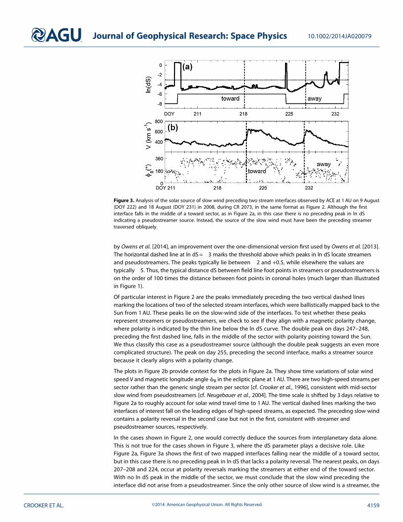
In the cases shown in Figure 2, one would correctly deduce the sources from interplanetary data alone.This is not true for the cases shown in Figure 3, where the dS parameter plays a decisive role. LikeFigure 2a, Figure 3a shows the first of two mapped interfaces falling near the middle of a toward sector,but in this case there is no preceding peak in ln dS that lacks a polarity reversal. The nearest peaks, on days207–208 and 224, occur at polarity reversals marking the streamers at either end of the toward sector.With no ln dS peak in the middle of the sector, we must conclude that the slow wind preceding theinterface did not arise from a pseudostreamer. Since the only other source of slow wind is a streamer, the

Figure 3. Analysis of the solar source of slow wind preceding two stream interfaces observed by ACE at 1 AU on 9 August(DOY 222) and 18 August (DOY 231) in 2008, during CR 2073, in the same format as Figure 2. Although the firstinterface falls in the middle of a toward sector, as in Figure 2a, in this case there is no preceding peak in ln dSindicating a pseudostreamer source. Instead, the source of the slow wind must have been the preceding streamertraversed obliquely.

Journal of Geophysical Research: Space Physics 10.1002/2014JA020079

CROOKER ET AL. ©2014. American Geophysical Union. All Rights Reserved. 4159

slow wind preceding the interface must have come from the preceding streamer on days 207–208,which reached central meridian 10 days earlier. This long period of time implies oblique passage throughthe streamer.

The interplanetary data in Figure 3b support the idea of oblique passage. The slow wind preceding thefirst interface extends all the way back to the polarity reversal on day 212, corresponding to the streamer onthe Sun spanning days 207–208. One might ask why ln dS in Figure 3a does not show a pattern of extendedelevated values corresponding to the extended slow speed in Figure 3b. A look at Figure 1 helps explainthis lack. There, dS has essentially two values—small and large. There are no boundary effects like the onesthat are assumed to give rise to slow wind [e.g., Riley and Luhmann, 2012]. The ln dS plot in Figure 3a does

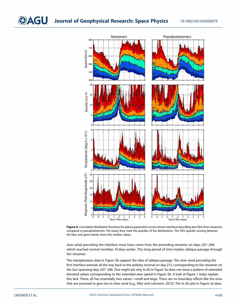
Figure 4. Cumulative distribution functions for plasma parameters across stream interfaces bounding slow flow from streamerscompared to pseudostreamers. The heavy lines mark the quartiles of the distributions. The 50% quartile running betweenthe blue and green bands traces the median values.

Journal of Geophysical Research: Space Physics 10.1002/2014JA020079

CROOKER ET AL. ©2014. American Geophysical Union. All Rights Reserved. 4160

hint at oblique passage, however, in the form of the flat-topped peaks. These successive high values indicateskimming near the heart of the streamer belt.

The long gap between the polarity reversal and the first interface in Figure 3 would preclude identificationof this event as a streamer case in any automated scheme trained to test whether an interface has anassociated polarity reversal using only interplanetary data, since the gap betweenmost interfaces and theirassociated polarity reversals is usually shorter than a day [Gosling et al., 1978]. The second interface inFigure 3 more nearly fits the usual streamer pattern. Although the gap between the mapped interface andthe polarity reversal in Figure 3a is over 2 days long, in Figure 3b, at 1 AU, the gap is roughly 1 day long.Thus, both interfaces in Figure 3 are classified as streamer cases. Consistent with this view is the fact thatFigure 3b displays only one stream per sector, in contrast to the two per sector in Figure 2b, where apseudostreamer brought slow wind mid-sector to create those two streams.

Examining the streamer identification parameter and the interplanetary data for each of the selected 128stream interface cases, as illustrated in Figures 2 and 3, we found that 84 met the criteria of a streamer caseand 44met the criteria of a pseudostreamer case. Superposed epoch analysis was then performed separately onthe two different kinds of cases. Figures 4 and 5 present the results in the form of cumulative distributionfunctions (cdfs).

Figure 4 displays cdfs of the variations of plasma parameters across the stream interfaces, from 5days beforeto 5 days after the crossing at zero epoch. The slow-wind side of the interfaces lies in the negative epochrange, as is clear from the speed cdfs in the top row. They indicate that the slowest winds occurred during the

Figure 5. Cumulative distribution functions for ionic and elemental composition parameters across stream interfaces in theformat of Figure 4.

Journal of Geophysical Research: Space Physics 10.1002/2014JA020079

CROOKER ET AL. ©2014. American Geophysical Union. All Rights Reserved. 4161

2 days preceding the interface (�2 to 0 epoch time), where the median (50%) speed contour dips down toabout 350 km/s in streamer flow compared to about 375 km/s in pseudostreamer flow, consistent withthe comparison in Crooker and McPherron [2012]. Also, apparent from �2 to 0 epoch is the larger spread ofspeed values for pseudostreamer flow, indicating greater variability compared to streamer flow. Comparisonof the density and proton temperature cdfs in the middle panels shows similar findings from �2 to 0 epochtime. The expected elevated density and depressed temperatures [e.g., Gosling et al., 1978] are slightlymore pronounced for streamer flow compared to pseudostreamer flow, consistent with the limited findingsof Neugebauer et al. [2004], and the variability for pseudostreamer flow is slightly higher. The cdfs formagnetic field magnitude in the bottom panel show a stronger peak at the interface for streamers comparedto pseudostreamers, consistent with the stronger speed gradient across the interface bounding streamers,which results in stronger compression.

Similar to Figure 4, Figure 5 displays cdfs of the variations of composition parameters across the interfaces.From �2 to 0 epoch time, both the ionic composition ratios of O7+/O6+ and C6+/C5+ and the elementalcomposition ratio of Fe/O are elevated, as expected [e.g., Wimmer-Schweingruber et al., 1997; Crooker andMcPherron, 2012], with slightly higher ratios for streamer flow compared to pseudostreamer flow, consistentwith the case studies ofWang et al. [2012]. Moreover, the broad width of the regions of characteristic slow flowin both streamers and pseudostreamers in Figures 4 and 5 suggests that the source mechanism proposed byWang et al. [2012], that is, a large expansion factor within coronal hole boundaries [e.g., Wang and Sheeley,1990], may contribute to the slow flows in addition to the competing source mechanism of opening large fluxloops through interchange reconnection [e.g., Fisk et al., 1998; Antiochos et al., 2011].

3. Discussion and Conclusions

The results in Figures 4 and 5 clearly show that pseudostreamer flows have the same characteristics asstreamer flow, that is, low speed and proton temperature and high density and composition ratio, but thatthese characteristics are slightly less pronounced in pseudostreamers. These findings raise two relatedissues, discussed below, regarding the speed of pseudostreamer flows and the concept of two kinds of solarwind—slow and fast.

One might argue that the slow speeds of pseudostreamer flows identified in this study were essentiallyguaranteed by the selection process, since the wind speed downstream of the impinging fast flow behind theinterface is always slow. By definition, interfaces are boundaries between fast and slow flow. It may wellbe that some pseudostreamer flows not included in this study are fast, as first predicted byWang et al. [2007].Occasionally, one can see high-speed segments in what otherwise is a slow-wind web on synoptic maps ofsolar wind speed predicted by the Wang-Sheeley-Arge model [Arge et al., 2004], but these appear to beuncommon. We conclude that the slow flows analyzed in this paper are typical of pseudostreamer flows.

On the other hand, the finding that in every way the pseudostreamer flow has less pronounced characteristicsthan streamer flow supports the idea that the solar wind comprises a continuum of dynamic states, asproposed by Zurbuchen et al. [2002] and inherent in the correlation between solar wind speed and O7+/O6+

[Fisk, 2003; Gloeckler et al., 2003]. The continuum stretches from the fastest winds from coronal holes to theslowest winds from streamers. Pseudostreamer flow can be said to represent the first step up fromstreamer flow in this continuum. The concept that solar wind is either slow or fast comes from the fact thatmuch of the time spacecraft are sampling wind near the extremes of the continuum. Only since thebeginning of the declining phase of solar cycle 23, in 2003, were pseudostreamer flows prevalent enoughto be identified as solar wind at a different position on the continuum.

ReferencesAntiochos, S. K., Z. Mikic, R. Lionello, V. Titov, and J. Linker (2011), A model for the sources of the slow solar wind, Astrophys. J., 731, 112,

doi:10.1088/0004-637X/731/2/112.Antiochos, S. K., J. Linker, R. Lionello, Z. Mikic, V. Titov, and T. H. Zurbuchen (2012), The structure and dynamics of the corona-heliosphere

connection, Space Sci. Rev., 172, 169–185, doi:10.1007/s11214-011-9795-7.Arge, C. N., J. G. Luhmann, D. Odstrcil, C. J. Schrijver, and Y. Li (2004), Stream structure and coronal sources of the solar wind during the May

12th, 1997 CME, J. Atmos. Terr. Phys., 66, 1295–1309.

Crooker, N. U., and R. L. McPherron (2012), Coincidence of composition and speed boundaries of the slow solar wind, J. Geophys. Res., 117,A09104, doi:10.1029/2012JA017837.

AcknowledgmentsYuming Wang thanks the reviewers fortheir assistance in evaluating this paper.

Journal of Geophysical Research: Space Physics 10.1002/2014JA020079

CROOKER ET AL. ©2014. American Geophysical Union. All Rights Reserved. 4162

Crooker, N. U., A. J. Lazarus, R. P. Lepping, K. W. Ogilvie, J. T. Steinberg, A. Szabo, and T. G. Onsager (1996), A two-stream, four-sector,recurrence pattern: Implications from WIND for the 22-year geomagnetic activity cycle, Geophys. Res. Lett., 23, 1275–1278, doi:10.1029/96GL00031.

Crooker, N. U., E. M. Appleton, N. A. Schwadron, and M. J. Owens (2010), Suprathermal electron flux peaks at stream interfaces: Signature ofsolar wind dynamics or tracer for open magnetic flux transport on the Sun?, J. Geophys. Res., 115, A11101, doi:10.1029/2010JA015496.

Crooker, N. U., S. K. Antiochos, X. Zhao, and M. Neugebauer (2012), Global network of slow solar wind, J. Geophys. Res., 117, A04104,doi:10.1029/2011JA017236.

Fisk, L. A. (2003), Acceleration of the solar wind as a result of the reconnection of open magnetic flux with coronal loops, J. Geophys. Res.,108(A4), 1157, doi:10.1029/2002JA009284.

Fisk, L. A., N. A. Schwadron, and T. H. Zurbuchen (1998), On the slow solar wind, Space Sci. Rev., 86, 51–60.Geiss, J., G. Gloeckler, and R. von Steiger (1995), Origin of the solar wind from composition data, Space Sci. Rev., 72, 49–60.Gloeckler, G., T. H. Zurbuchen, and J. Geiss (2003), Implications of the observed anticorrelation between solar wind speed and coronal

electron temperature, J. Geophys. Res., 108(A4), 1158, doi:10.1029/2002JA009286.Gosling, J. T., J. R. Asbridge, S. J. Bame, and W. C. Feldman (1978), Solar wind stream interfaces, J. Geophys. Res., 83, 1401–1412, doi:10.1029/

JA083iA04p01401.Neugebauer, M., P. C. Liewer, B. E. Goldstein, X. Zhou, and J. T. Steinberg (2004), Solar wind stream interaction regions without sector

boundaries, J. Geophys. Res., 109, A10102, doi:10.1029/2004JA010456.Owens, M. J., N. U. Crooker, and M. Lockwood (2013), Solar origin of heliospheric magnetic field inversions: Evidence for coronal loop

opening within pseudostreamers, J. Geophys. Res. Space Physics, 118, 1868–1879, doi:10.1002/jgra.50259.Owens, M. J., N. U. Crooker, and M. Lockwood (2014), Solar cycle evolution of dipolar and pseudostreamer belts and their relation to the slow

solar wind, J. Geophys. Res. Space Physics, 119, 36–46, doi:10.1002/2013JA019412.Riley, P., and J. G. Luhmann (2012), Interplanetary signatures of unipolar streamers and the origin of the slow solar wind, Sol. Phys., 277,

355–373, doi:10.1007/s11207-011-9909-0.Wang, Y.-M., and N. R. Sheeley Jr. (1990), Solar wind speed and coronal flux-tube expansion, Astrophys. J., 355, 726.Wang, Y.-M., N. R. Sheeley Jr., and N. B. Rich (2007), Coronal pseudostreamers, Astrophys. J., 658, 1340–1348.Wang, Y.-M., R. Grappin, E. Robbrecht, and N. R. Sheeley Jr. (2012), On the nature of the solar wind from coronal pseudostreamers, Astrophys.

J., 749, 182–195, doi:10.1088/0004-637X/749/2/182.Wimmer-Schweingruber, R. F., R. von Steiger, and R. Paerli (1997), Solar wind stream interfaces in corotating interaction regions: SWICS/

Ulysses results, J. Geophys. Res., 102, 17,407–17,417, doi:10.1029/97JA00951.Zhao, L., and L. Fisk (2011), Understanding the behavior of the heliospheric magnetic field and the solar wind during the unusual solar

minimum between cycles 23 and 24, Solar Phys., 274, 379–397, doi:10.1007/s11207-011-9840-4.Zhao, L., T. H. Zurbuchen, and L. A. Fisk (2009), Global distribution of the solar wind during solar cycle 23: ACE observations, Geophys. Res.

Lett., 36, L14104, doi:10.1029/2009GL039181.Zurbuchen, T. H., L. A. Fisk; G. Gloeckler, and R. von Steiger (2002), The solar wind composition throughout the solar cycle: A continuum of

dynamic states, Geophys. Res. Lett., 29(9), 1352, doi:10.1029/2001GL013946.

Journal of Geophysical Research: Space Physics 10.1002/2014JA020079

CROOKER ET AL. ©2014. American Geophysical Union. All Rights Reserved. 4163