vy902033/papers_pdfs/2014... · galactic cosmic ray modulation near the heliospheric current sheet...

1 23

�� !��"�#"��$%�""&�$��"'��'��

��

��

1 23

Your article is protected by copyright and allrights are held exclusively by Springer Science+Business Media Dordrecht. This e-offprintis for personal use only and shall not be self-archived in electronic repositories. If you wishto self-archive your article, please use theaccepted manuscript version for posting onyour own website. You may further depositthe accepted manuscript version in anyrepository, provided it is only made publiclyavailable 12 months after official publicationor later and provided acknowledgement isgiven to the original source of publicationand a link is inserted to the published articleon Springer's website. The link must beaccompanied by the following text: "The finalpublication is available at link.springer.com”.

Solar PhysDOI 10.1007/s11207-014-0493-y

Galactic Cosmic Ray Modulation near the HeliosphericCurrent Sheet

S.R. Thomas · M.J. Owens · M. Lockwood · C.J. Scott

Received: 9 September 2013 / Accepted: 3 February 2014© Springer Science+Business Media Dordrecht 2014

Abstract Galactic cosmic rays (GCRs) are modulated by the heliospheric magnetic field(HMF) both over decadal time scales (due to long-term, global HMF variations), and overtime scales of a few hours (associated with solar wind structures such as coronal mass ejec-tions or the heliospheric current sheet, HCS). Due to the close association between the HCS,the streamer belt, and the band of slow solar wind, HCS crossings are often associated withcorotating interaction regions where fast solar wind catches up and compresses slow solarwind ahead of it. However, not all HCS crossings are associated with strong compressions.In this study we categorize HCS crossings in two ways: Firstly, using the change in magneticpolarity, as either away-to-toward (AT) or toward-to-away (TA) magnetic field directions rel-ative to the Sun and, secondly, using the strength of the associated solar wind compression,determined from the observed plasma density enhancement. For each category, we use su-perposed epoch analyses to show differences in both solar wind parameters and GCR fluxinferred from neutron monitors. For strong-compression HCS crossings, we observe a peakin neutron counts preceding the HCS crossing, followed by a large drop after the crossing,attributable to the so-called ‘snow-plough’ effect. For weak-compression HCS crossings,where magnetic field polarity effects are more readily observable, we instead observe thatthe neutron counts have a tendency to peak in the away magnetic field sector. By splittingthe data by the dominant polarity at each solar polar region, we find that the increase in GCRflux prior to the HCS crossing is primarily from strong compressions in cycles with negativenorth polar fields due to GCR drift effects. Finally, we report on unexpected differences inGCR behavior between TA weak compressions during opposing polarity cycles.

Keywords Cosmic rays · Heliospheric current sheet · 22-year cycle · Energetic particles

1. Introduction

In 2009 – 2010, the heliospheric magnetic field (HMF) intensity reached its lowest value ofthe space age, which is taken here to be approximately 1965 onwards (Owens et al., 2011;

S.R. Thomas (B) · M.J. Owens · M. Lockwood · C.J. ScottUniversity of Reading, Reading, UKe-mail: [email protected]

Author's personal copy

mailto:[email protected]

S.R. Thomas et al.

McComas et al., 2012; Lockwood et al., 2012). Simultaneously, near-Earth galactic cosmicray (GCR) fluxes, inferred from ground-based neutron monitors, peaked at their highest val-ues over the same period (Aslam and Badruddin, 2012; Krymsky et al., 2012), as the HMFmodulation effects were weaker (Thomas, Owens, and Lockwood (2013) and referencestherein). Near-Earth GCR flux can also be inferred from cosmogenic isotopes containedwithin ice sheets and biomass, allowing the reconstruction of HMF before neutron monitorswere in use (e.g. McCracken et al., 2004; Steinhilber, Beer, and Frohlich, 2009; Steinhilberet al., 2010; Usoskin, Bazilevskaya, and Kovaltsov, 2011; Lockwood et al., 2012; Owens,Usoskin, and Lockwood, 2012). On shorter time scales, understanding the heliospheric mod-ulation of GCRs is necessary both to interpret the cosmogenic isotope data and to explainchanges seen at Earth, such as those in atmospheric electricity (e.g. Scott et al., 2013), andthe effects on modern operational systems such as electronics on satellites and aircraft.

GCR fluxes at Earth are known to be modulated by a variety of different processes withinthe heliosphere (e.g. McCracken and Ness, 1966). As they travel through the heliospherethey are subject to drift effects, scattering from irregularities, diffusion, and adiabatic de-celeration (Parker, 1965). During the 11-year cycle in sunspot number, the Sun’s dominantmagnetic polarity reverses around the time of solar maximum, which is predicted to have asignificant effect on GCR modulation through average particle drift patterns (Jokipii, Levy,and Hubbard, 1977). By convention, the polarity of the solar field qA (where q is the chargeon the energetic particle and A is the direction of the solar global field) is taken to be neg-ative when the dominant polar field is inward in the northern hemisphere and outward inthe southern, whereas qA is positive if the opposite is true (e.g. Ahluwalia, 1994). Jokipii,Levy, and Hubbard (1977) suggested that particle drifts differ during different qA cycles,with GCR protons reaching Earth from drifting down from the solar poles during qA > 0cycles, whereas in qA < 0 they arrive at Earth down the heliospheric current sheet (HCS).This gives rise to a 22-year cycle in near-Earth GCR flux (Hale and Nicholson, 1925), andhas been used to explain alternate ‘peak’ and ‘dome’ maxima in the neutron count timeseries.

The HCS separates regions of opposing HMF polarity and lies close to the ecliptic planearound times of solar minimum (Hoeksema, Wilcox, and Scherrer, 1983; Tritakis, 1984),becoming more warped as solar activity increases. The modulation of GCRs by the HCShas been studied in the long term by Paouris et al. (2012) and Mavromichalaki and Paouris(2012). They showed that the long-term variation in GCR modulation can be modeled usinga number of solar and heliospheric variables, including the tilt angle of the HCS relative tothe solar rotation direction, and showed a significant correlation between HCS tilt angle andthe GCR modulation parameter during recent solar cycles.

The HCS passes over Earth a number of times (usually between two and six times) per27-day rotation (e.g. Smith, 2001). HCS crossings provide an excellent opportunity to sam-ple GCR flux in opposite magnetic polarities at the same stage of the solar cycle and undersimilar solar wind conditions. However, HCS crossings are often associated with corotatinginteraction regions (CIRs) (e.g. Tsurutani et al., 1995), due to the HCS’s close associationwith the streamer belt and the band of slow solar wind. These are relevant to the present studyas they modulate the GCR flux (for example, Rouillard and Lockwood, 2007). The presenceof a CIR in spacecraft measurements is seen as an increase in the solar wind plasma densityand magnetic field intensity resulting from the compression of slow solar wind streams bythe fast wind behind them. The increased field in this compressed region acts as a barrierto GCR propagation giving enhanced fluxes ahead of it and reduced fluxes behind it, oftenreferred to as the ‘snow plough effect’.


Galactic Cosmic Ray Modulation near the Heliospheric Current Sheet

Badruddin, Yadav, and Yadav (1985) separated HCS crossings into away-to-toward (AT)and toward-to-away (TA) magnetic fields, where toward/away sectors are defined as mag-netic field lines following a Parker spiral magnetic field directed, towards/away from theSun, respectively. They considered the period from 1964 to 1976 and split the data intothree periods; the solar minimum between cycles 20 and 21, the maximum of cycle 21,and the minimum between cycles 21 and 22. For a range of different neutron monitor sta-tions they found that, on average, neutron counts peaked as the HCS crossed Earth and thendecreased to a value lower than that before the crossing. Badruddin and Ananth (2003) ex-tended the study period to 1985, essentially including a second solar cycle, and concludedthat GCR flux is more strongly affected during qA > 0 cycles; a finding also noted by ElBorie, Duldig, and Humble (1998). They also noted a greater increase in GCRs across ATthan TA crossings. Further to this, Richardson, Cane, and Wibberenz (1999) have foundthat the response of GCRs to modulation by recurrent CIRs is 50 % greater in qA > 0 thanqA < 0 cycles during two solar minimum periods in the mid-1950s and mid-1990s.

El Borie (2001) compared data from cycles 21 and 22. He first noted differences in appar-ent propagation characteristics of GCRs between the recovery and declining phases of thesolar cycle, including a rigidity dependence of the variation. Furthermore, he notes that GCRflux varies more during toward magnetic field polarity days compared with during away po-larity days. However, in each of these investigations, the data available to him only includedup to two solar cycles, compared with the four cycles available now. In this study, we aimto add to the two solar cycles used in e.g. El Borie, Duldig, and Humble (1998) and furthersplit the data based upon the strength of the solar wind compression associated with eachHCS crossing. The aim is to attempt to separate the ‘magnetic barrier’ (or ‘snow-plough’)effect from any effect resulting purely from different magnetic polarities either side of theHCS crossing.

In Section 2 we identify all HCS crossings in the period 1965 – 2013. This HCS catalogueis used in Section 3 to deduce the average variations in GCR flux over all HCS crossings.

2. Identifying Current Sheet Crossings

In this section, we produce a catalogue of HCS crossings over the period from 1964 to2012 from the OMNI-2 dataset (King and Papitashvili, 2005) of near-Earth solar wind ob-servations. Each crossing is identified by the change in in-ecliptic magnetic field angle, φB ,derived from the geocentric solar ecliptic (GSE) x- and y-components from an ideal Parkerspiral angle assuming a constant solar wind speed, of approximately 135◦ to one of 315◦ orvice versa, similar to the method used by El Borie (2001) and Badruddin, Yadav, and Yadav(1985). We do not include HCS crossings in which the magnetic field rotates smoothly orfluctuates between regimes, but we rather limit event selection to those that display a sharptransition within a duration of approximately 1 h. This reduces the size of the catalogue, butit reduces uncertainty in the time of the HCS crossing and means that we are studying quasi-tangential discontinuities (with only a small or zero field threading the structure) rather thanrotational discontinuities. The orientation of the HCS crossing (i.e. whether the direction ofmagnetic field lines change from AT or TA) is deduced from the sign of the magnetic fieldcomponent, Bx , in the direction of the Sun from Earth.

A typical HCS crossing is shown in Figure 1. The panels, from top to bottom, showthe neutron monitor counts, the in-ecliptic magnetic field angle, the y-component of solarwind velocity, the solar wind velocity in the x-direction (this is negative in sign so we takethe magnitude to display an increase in speed as being positive), the HMF intensity |B|,


S.R. Thomas et al.

Figure 1 A typical HCS crossing centered on 23 December 1999. From top; neutron counts, in-eclipticmagnetic angle of magnetic field, solar wind velocity component in the y-direction, solar wind speed in thex-direction, heliospheric magnetic field magnitude, HMF in the x-direction, and plasma density. The verticaldashed line indicates the HCS crossing defined by the change in magnetic angle. The horizontal orange linesdisplay the ideal in-ecliptic magnetic field angles.

the x-component of the HMF and plasma density. Ten days of data centered on 23 Decem-ber 1999 are shown, with the HCS crossing at time 0. The neutron monitor data shown wererecorded at McMurdo (magnetic latitude of 77.9 South), which has been collecting datasince 1964 (e.g. Kruger et al., 2008). McMurdo’s location near the south pole is ideal asit provides increased sensitivity to heliospheric modulation effects, due to reduced shield-ing by the terrestrial magnetic field (Bieber et al., 2004). However, similar results wereconsistently found at other stations, including northern hemisphere stations such as Thule,Greenland (magnetic latitude of 76.5 North, not shown).

In Figure 1 we show the variation of each parameter in hourly values for five days eachside of the crossing. In the top panel we see a steady increase in the neutron monitor counts,until approximately the time of the crossing, where it decreases slightly before leveling off.By comparing the in-ecliptic magnetic field angle to the ideal Parker spiral angles (com-puted assuming a steady solar wind speed of 400 km s−1 and shown in orange, this angledoes not change much for typical solar wind speeds), the second panel from the top showsthe HCS crossing as a rapid change from 135◦ to 315◦. The fifth panel shows that Bx changesfrom negative to positive and so this is an AT crossing. The y-component of the solar windvelocity is given in the third panel and shows a reversal from negative velocity to posi-



tive across the HCS, consistent with the flow deflection at a stream interface (Borovskyand Denton, 2010). The magnitude of the radial solar wind velocity, vx , increases over thecrossing, as does Bx in agreement with the spiral angle increase. We see large peaks in theHMF intensity and the plasma density at the HCS crossing, associated with the compressionregion.

We searched for events with a similar reversal in spiral angle, throughout the whole1 h resolution OMNI-2 dataset and found a total of 1950 events. Including data gaps, thisequates to an equivalent of one HCS crossing every nine days. However, removing datagaps and unclear HCS crossings due to extended rotations in the in-ecliptic magnetic fielddirection (perhaps owing to the presence of coronal mass ejections at the HCS; e.g. Crookeret al., 1998) reduced the event list to 402 HCS crossings, approximately one event per 45days. Thus, the more conservative criterion for event identification we have adopted meansthat the rate of events studied is much lower than that used in El Borie (2001) who compiled71 events in a three-year period and 108 in four years during a later period for their study,and also than Badruddin, Yadav, and Yadav (1985) and Badruddin and Ananth (2003) whorestricted their catalogue to those where the polarity did not change for at least five daysbefore and after the HCS crossings.

3. Cosmic Ray Variations Associated with Current Sheet Crossings

We now look at solar wind and GCR variations across the HCS statistically. Figure 2 showsa superposed epoch study (also called a ‘Chree analysis’ or a ‘composite’), using the HCScrossing as the zero epoch time, denoted t0, and showing the percentage change in neu-tron counts (discussed further below), the solar wind speed, plasma density and HMF fieldstrength as a function of epoch time, te (= t − t0), between five days before and five daysafter the HCS crossing. The mean variation is shown as the orange lines in Figure 2.

The significance of any variations in the means are tested by a Monte-Carlo approach, inwhich we repeat the exact same analysis, but for 402 randomly selected zero epoch times,rather than 402 HCS crossing times. This process is repeated 1000 times to generate 1000random means at every epoch time. The resulting Monte-Carlo mean is shown by the blackline in Figure 2, and the bounds between which 90 % of the random epoch time means arecontained are displayed as the grey shaded region (i.e., the upper and lower bands are the5 % and 95 % confidence intervals). Thus HCS crossings generate variations in the observedproperties which are significant at every epoch time (above the 95 % confidence level) aboverandom fluctuations at times when the observed mean lies outside of the shaded band. Thistest has been applied on all further figures in the article.

We first concentrate on the heliospheric parameters shown in Figure 2. The significantpeaks in the plasma density (top right) and HMF intensity (bottom left) herald the presenceof the compression regions expected by the association of the HCS with CIRs. Here, thetypical peak in density is approximately 14 cm−3 compared with the average backgrounddensity of 6 cm−3 and the HMF intensity increases from approximately 5.2 nT to 8.2 nT.We note the large reduction in radial solar wind speed, to an average of 360 km s−1 beforea steep rise to 460 km s−1. This clearly shows the presence of a transition from slow solarwind to fast wind as the HCS passes the spacecraft. Similar patterns at stream interfaces,where slow proceeds fast wind, were shown in these variables by Crooker and McPherron(2012).

Neutron monitor counts show solar cycle variations much larger than typical variationsacross the HCS. Therefore, in order to compose a superposed epoch analysis of GCR flux


S.R. Thomas et al.

Figure 2 Superposed epoch analysis for all clear HCS crossings within the four solar cycles (orange lines)showing (a) percentage change in neutron counts, (b) plasma density, (c) magnitude of the heliospheric mag-netic field, and (d) radial solar wind velocity. The black lines are the means of the Monte-Carlo analysis usingrandom event times and the shaded regions are the 95 % and 5 % confidence bands. The vertical dashed linesshow the zero epoch time of the HCS crossing [t0]. The number of events are given in the boxes in the topright of each panel.

variations associated with HCS crossings, it is necessary to normalize the neutron counts.We take a background value of each parameter defined as the mean of hourly values fromfive days before to five days after the HCS crossing time, but excluding 12 h each side ofthe crossing itself. From this, we compute the percentage change in neutron monitor countsrelative to the background. Any changes above 20 % are attributed to large solar energeticparticle (SEP) events and removed from the dataset (Barnard and Lockwood, 2011). How-ever, this only reduces the data size by approximately 0.5 %. Figure 2 (top left) shows a su-perposed epoch analysis of percentage change in neutron counts relative to the backgroundlevel for all HCS crossings in the four solar cycles considered in the study. On average wesee a peak in neutron counts of 0.35 % over the background just before the HCS crossesthe spacecraft, which is considerably greater than the 95 % confidence level. Following theHCS crossing the neutron counts are depressed but this only exceeds the 95 % significancelevel after about four days following the crossing.

In general, on long time scales, neutron counts are known to be modulated by the HMF.Therefore, if this applied on all time and spatial scales, the profile of the neutron counts



Figure 3 Superposed epoch analyses of the percentage change in neutron counts from the background (redlines): (a) means of away-to-toward HCS crossings and (b) toward-to-away HCS crossings. The black linesagain are the means of the Monte Carlo analysis using random event times and the shaded region is the 95 %confidence band, and the vertical line is the zero epoch time.

would appear as the inverse of the magnitude of the HMF. However, the peak and troughof the neutron counts are not located at the same time as the trough and peak of the HMFstrength, respectively. This behavior is due to the snow-plough effect where, as a region ofcompressed magnetic field propagates out through the heliosphere, it pushes a region of en-hanced energetic particle flux in front of it, with a region of depleted GCR flux immediatelybehind it (e.g. Richardson, 2004).

Figure 3 shows the corresponding results for the same dataset split into AT and TA events.Here Figure 3a shows the AT HCS crossings and Figure 3b shows TA crossings. Again,a Monte-Carlo analysis is applied and the 95 % confidence interval shown by the shadedregion. The heliospheric parameters are not included here but show the same patterns as inFigure 2 (i.e. there are no systematic differences in the solar wind compression characteris-tics for TA and AT events).

Comparing Figures 3a and 3b we note differing behavior in GCR flux between the AT andTA cases. The GCR flux in the AT case shows a build up in GCR flux peaking approximately


S.R. Thomas et al.

a day before t0, whereas the GCR flux peaks almost symmetrically over t0 in the TA case.There are also notable differences in the days following the HCS crossing. The GCR fluxafter an AT HCS crossing falls off steeply to an approximately 95 % significant depletion ofGCRs from one to four days after the crossing. However, after the TA HCS crossings, theGCR flux decreases more gradually and does not reach a 95 % significance level depletionuntil over four days after the crossing.

4. Effect of Solar Wind Compression on Neutron Counts

As discussed above, HCS crossings are often associated with a transition between slow andfast solar wind (e.g. Thomas and Smith, 1981). The resulting compression, which oftenforms a CIR, can frequently result in increased plasma density and HMF intensity. Thus, thelocal strength of the compression front in the heliosphere can be estimated on the basis ofthe plasma density and magnetic field intensity enhancement observed in near-Earth space.We therefore here divide the HCS into ‘strong’ (SCC) and ‘weak’ (WCC) compressioncrossings on this basis.

For each HCS crossing, the magnitude of the maximum in plasma density within 2.5 daysof the HCS crossing is compared with the background value, defined in the same manneras the neutron counts background, above. A plasma density greater than three times thebackground value is taken to constitute a strong compression, whereas a plasma density lessthan three times the background is here classed as a weak compression. Splitting the data inthis way results in 271 strong compressions and 131 weak compressions.

Superposed epoch analyses of the plasma density and magnetic field intensity for SCCs(top panels) and WCCs (bottom panels), are displayed in Figure 4. The orange lines hereshow the mean value of each epoch and the shaded region and black lines are again theresults of a Monte-Carlo analysis with 95 % of 1000 randomly selected events within theshaded region.

Events that we define as SSCs here (Figures 4a and 4b) have large, sharp peaks in plasmadensity, np, and a significant increase in HMF intensity, |B|, well outside of the 95 % signif-icance level. However, the events in Figure 4c found to have low plasma density enhance-ments, also have low magnetic field intensity enhancements (shown in Figure 4d). Here,a weak depression before the HCS crossing is seen to evolve slowly to a weak enhancementafter it. The depression and enhancement in the HMF both still exceed the 95 % confidencelevel but they crucially have a much smaller magnetic field enhancement at around the zeroepoch time. In other words, the WCCs are, unlike the SCCs, not associated with a strongmagnetic barrier. Reducing the threshold for weak events any further would mean that thereis not a large enough sample, but note that the threshold used means a magnetic barrier ispresent in WCC cases, on average, albeit a much weaker one.

Figure 5 repeats the analysis of Figure 3, but it subdivides the dataset into strong- andweak-compression HCS crossings. The same format is applied as from previous figures.Figures 5a and 5b show AT and TA SCCs whereas Figures 5c and 5b show AT and TAWCCs, respectively. Note that compared with Figure 3, the width of the 95 % confidencebands has increased, due to the reduced sample size from the subdivision of the dataset.

There are a number of points of note. Firstly, Figure 3a shows that in the AT case, a peakin neutron counts occurs approximately a day before the HCS crossing. The AT HCS cross-ings in Figures 5a (strong compressions) and 5c (weak compressions) both show the samecharacteristics, where the peak in neutron counts occurs before the HCS crossing (i.e. whent < te). However, Figure 3b showed a peak in neutron counts for the TA case which is ap-proximately symmetrical across t0. Figures 5b and 5d do not peak at the same te. Therefore,



Figure 4 Left: Means of solar wind plasma density (orange lines), np, during: (a) strong-compression HCScrossings and (c) weak-compression HCS crossings. HMF intensity during: (b) strong-compression HCScrossings and (d) weak-compression HCS crossings. The Monte-Carlo analyses are again shown. The numberof events for each row is given in the top right of each plot and the vertical lines are the zero epoch times.

it is clear that Figure 3b is made from a combination of an increase before the HCS crossingsin the strong-compression case (Figure 5b) and an increase in neutron counts after the cross-ing in the weak-compression case (Figure 5d), as these curves are approximately a mirrorimage of each other across the HCS crossing.

Secondly, the SCCs (Figures 5a and 5b) both have similar characteristics. The neutroncounts are seen to increase to a maximum before the HCS crossing and then to decreaseacross it to a minimum later in the time period. Again, the neutron counts are significantlydepleted between one and four days after the HCS crossing in the AT case (Figure 5a) butare seen to drop out of the 95 % significance after approximately three days in the TA case(Figure 5b).

The WCCs show a different pattern, however. By largely removing the strong magneticbarrier associated with strong compressions, we can better observe any effect of the changein magnetic polarity. Figure 5c shows a significant enhancement in GCR flux prior to the ATHCS crossing, which gradually reduces throughout the rest of the time period. Figure 5d,however, shows a large peak in neutron counts after the TA HCS crossing. This peak isapproximately a day later than for the AT case, although the increase is greater in the TAcase from a significant depletion at three days before the HCS crossing. A result of this is


S.R. Thomas et al.

Figure 5 Red lines display the percentage change in neutron counts across HCS crossings. Strong compres-sions are shown in the top panels (a and b) and weak compressions at the bottom (c and d). Again the blackline and shaded regions are the mean and spread of the Monte-Carlo runs. The number of events in eachepoch is given in the top right of each panel and the vertical line is the zero epoch time.

that there is, in general, an increase in GCR flux in the away magnetic field sector, withinthe vicinity of the HCS.

Heliospheric parameters such as the HMF intensity were also split into AT and TA HCScrossings and it was found that there are no difference in the timing of the peak in HMFintensity between these cases (not shown). Therefore, any difference between AT and TAHCS crossings cannot be directly attributed to any difference in the HMF or plasma densityand so is associated with the field polarities.

5. Effect of Solar Polarity Reversals

In this section, we investigate GCR variations across the HCS in different solar polaritycycles. The difference in direction of the propagation of GCRs through the heliosphere,as suggested by Jokipii, Levy, and Hubbard (1977), would be expected to cause a differ-ence in their behavior across the HCS. During qA < 0 cycles, the northern polar magneticfield is toward the Sun and GCRs are predominantly reaching Earth along the HCS from



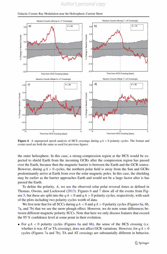
Figure 6 A superposed epoch analysis of HCS crossings during qA < 0 polarity cycles. The format andevents used are both the same as used for previous figures.

the outer heliosphere. In this case, a strong-compression region at the HCS would be ex-pected to shield Earth from the incoming GCRs after the compression region has passedover the Earth, because then the magnetic barrier is between the Earth and the GCR source.However, during qA > 0 cycles, the northern polar field is away from the Sun and GCRspredominantly arrive at Earth from over the solar magnetic poles. In this case, the shieldingmay be earlier as the barrier approaches Earth and would not be a large factor after is haspassed the Earth.

To define the polarity, A, we use the observed solar polar reversal times as defined inThomas, Owens, and Lockwood (2013). Figures 6 and 7 show all of the events from Fig-ure 5, but these are split into the qA < 0 and qA > 0 polarity cycles, respectively, with eachof the plots including two polarity cycles worth of data.

We first note that for all SCCs during qA < 0 and qA > 0 polarity cycles (Figures 6a, 6b,7a, and 7b) that we see the snow-plough effect. However, we do note some differences be-tween different magnetic polarity SCCs. Note that here we only discuss features that exceedthe 95 % confidence level at some point in their evolution.

• For qA < 0 polarity cycles (Figures 6a and 6b), the sense of the HCS crossing (i.e.whether it was AT or TA crossing), does not affect GCR variations. However, for qA > 0cycles (Figures 7a and 7b), TA and AT crossings are substantially different in behavior,


S.R. Thomas et al.

Figure 7 A superposed epoch analysis of HCS crossings during qA > 0 polarity cycles. Format is again thesame as previous figures.

as TA crossings appear to be a much greater barrier to GCRs than we observes at ATcrossings.

• For AT events, there is a polarity cycle effect, where the ‘snow-plough effect’ is muchstronger during qA < 0 polarity cycles (Figure 6a) than during qA > 0 cycles (Figure 7a).

• For TA events, we also see a polarity cycle effect, although this is different in behavior tothe effect seen between AT events. qA < 0 polarity cycles show a build up similar thanfor the AT case (Figure 6b). However, during qA > 0 polarity cycles we see a significantenhancement in GCR flux prior to the HCS and lasting from 3.5 days before the HCScrossing to a day afterwards (Figure 7b).

For WCCs, in general, the difference in solar polarity and the sense of the HCS crossingsall seem to affect GCR variations. We shall now discuss some key features of the WCCs(Figures 6c, 6d, 7c, and 7d).

• AT HCS crossings are an exception to this rule (Figures 6c and 7c), in that the solar polar-ity does not have an obvious effect. In both cases there is a GCR variation in agreementwith a weak snow-plough effect due to the associated weak magnetic field enhancement.

• However, for TA crossings during qA > 0 polarity cycles (Figure 7d), there is a strongenhancement in GCR flux, which is roughly symmetrical about the HCS crossings. This



enhancement is roughly in agreement with the enhancement in Figure 7b, but it does notbegin so early with respect to the HCS.

• For TA crossings during qA < 0 polarity cycles (Figure 6d), there is a very differentvariation in the behavior of GCRs. Here there is a significant depletion to the 95 % levelin GCRs from five to three days before the HCS crossing, which increases in almost astep-change just prior to the crossing to a significant enhancement in GCR flux from t0 tothree days after the crossing.

• Finally, we note that qA < 0 cycles do show a tendency for greater GCR flux in awaysectors. However, this difference is much less pronounced than in qA > 0 cycles, whereGCR flux enhancement is almost symmetric across the HCS crossing.

6. Discussion and Conclusions

To analyze the behavior of GCRs across heliospheric current sheet (HCS) crossings we havecollected 402 clear instances where the HCS has crossed Earth. We have used superposedepoch analyses to look at small but systematic trends that may otherwise be swamped byevent-to-event variability and noise when considering a single case study. Approximatelyhalf of the identified HCS crossings are away-to-toward (AT) with the other half beingtoward-to-away (TA) magnetic field directions. We have also divided these events into‘strong’ and ‘weak’ compression HCS crossings. Splitting the data in this way allows usto separate the effects of large compression regions, which act as a barrier to GCR propa-gation, and changing magnetic polarity from AT or TA. We shall now summarize our keyfindings and discuss their implications.

• When splitting the data into AT and TA HCS crossings, we find that the GCR flux at ATHCS crossings peaks approximately a day before the HCS crossings for AT crossings butis centred over the HCS for TA crossings. There is no variation in the timing of the peakin the intensity of the heliospheric magnetic field or plasma density between AT and TAHCS crossings to account for this difference.

• Strong-compression HCS crossings (SCCs) always display the ‘snow-plough effect’, in-dependent of HCS crossing being AT or TA, and in general show a greater variationthan weak-compression crossings (WCCs). This effect is associated with CIRs, where theGCR flux is known to peak shortly before the HCS crossing, followed by a large depletionin GCRs after the barrier has passed through owing to the scattering off inhomogeneitieswithin the CIR as it moves out through the heliosphere (Richardson, 2004). These generalresults are consistent with previous findings (e.g. Badruddin, Yadav, and Yadav, 1985; ElBorie, Duldig, and Humble, 1998; Richardson, 2004).

• To reduce the dominant effect of the barrier in SCCs, WCCs need to be considered whenobserving the differing behavior of GCR flux between AT and TA HCS crossings. SCCsshow similar behavior independent of the sense of the HCS crossing, but for WCCs, ATand TA crossings are not the same. The peak in GCR flux occurs after HCS crossings inthe TA case but is seen before the HCS in the AT case. We propose that this different be-tween toward and away sectors is due to the ease in which the GCRs can access magneticfield lines in each polarity. GCR drift effects as described by Jokipii, Levy, and Hubbard(1977), however, do not appear to be the direct cause, as there are more GCRs within theaway sector independent of polar polarity.

• When splitting the data further into polarity cycles, it is seen that all SCCs show the‘snow-plough effect’ to some degree. For AT events, we see a much greater variation inGCR flux across the HCS during qA < 0 polarity cycles than for those during qA > 0


S.R. Thomas et al.

cycles. This is in agreement with drift effects as described by Jokipii, Levy, and Hubbard(1977). During qA < 0, GCRs drift to Earth from the outer heliosphere down the HCS. Asthe HCS approaches, GCR flux is likely to increase due to scatter from the approachingmagnetic field enhancement. However, as GCRs drift from over the solar poles to Earthduring qA > 0 cycles, then this effect is unlikely to be as strong.

• For TA events, we also find a polarity cycle difference, but this is different from that seenfor AT events. One would expect a larger ‘snow-plough effect’ from HCS crossings duringqA < 0 than qA > 0 polarity cycles from drift effect, but instead we see a large and long-lasting enhancement from 3.5 days to the time of the crossing during qA > 0 polarities.Although drift effects appear not to be the cause, the reason for this enhancement is notclear.

• For AT WCCs in both solar magnetic polarities, we see evidence of a weak ‘snow-plougheffect’ due to the weak but significant increase in the heliospheric magnetic field intensity.

• TA WCCs show a very different variation in GCR flux depending on solar polarity. DuringqA > 0 polarity cycles, these show an almost symmetrical, large peak across the HCS.The overall pattern is not similar to the AT case but is compared to the SCCs case, butwithout the early increase in GCR flux. On the other hand, during qA < 0 polarity cycles,we observe a strong step increase in GCR flux from before the HCS to after it, with moreGCRs present within the away-from-the-Sun magnetic field lines. The causes of thesebehaviors is not clear, although it is worth noting that there are only 35 events in thesesuperposed epoch analyses and so sample sizes have decreased but the division of thedata.

• Although we agree with key conclusions of previous studies (e.g. El Borie, Duldig, andHumble, 1998; Richardson, Cane, and Wibberenz, 1999), we find a number of notabledifferences. For example, El Borie, Duldig, and Humble (1998) found a larger percentageincrease across the HCS crossing than we report, with the peak in GCR flux occurringapproximately a day later for AT than TA HCS crossings, where in fact we note theopposite behavior. Our results also differ from those of Badruddin and Ananth (2003) andEl Borie, Duldig, and Humble (1998) as we do not see evidence of a greater degree ofGCR modulation during qA > 0 cycles than during qA < 0 cycles. Furthermore, we notethat for TA WCCs, GCR flux is considerably greater in the away sector during qA < 0cycles but there is little difference during qA > 0 cycles. These differences may arise aswe have been very conservative when selecting HCS crossings and consequently haveselected fewer HCS crossing events per year. However, this has been compensated for, interms of numbers of events, because we have considered a longer period including fourpolarity cycles, compared to their two or three available cycles at the time.

Acknowledgements We are grateful to the Space Physics Data Facility (SPDF) of NASA’s Goddard SpaceFlight Centre for combining the data into the OMNI 2 dataset which was obtained via the GSFC/SPDF OM-NIWeb interface at http://omniweb.gsfc.nasa.gov. We also thank the Bartol Research Institute of the Uni-versity of Delaware for the neutron monitor data from McMurdo, which is supported by NSF grant ATM-0527878. The work of SRT is supported by a studentship from the UK’s Natural Environment ResearchCouncil (NERC).

References

Ahluwalia, H.S.: 1994, Cosmic ray transverse gradient for a Hale Cycle. J. Geophys. Res. 99, 23515 – 23521.Aslam, O.P.M., Badruddin: 2012, Solar modulation of cosmic rays during the declining and minimum phases

of solar cycle 23: Comparison with past three solar cycles. Solar Phys. 279, 269 – 288.Badruddin, Ananth, A.G.: 2003, Variation of cosmic ray intensity with angular distance from Earth to the

current sheet. In: 28th Int. Cosmic Ray Conf., 3909 – 3912.


http://omniweb.gsfc.nasa.gov


Badruddin, Yadav, R.S., Yadav, N.R.: 1985, Intensity variation of cosmic rays near the heliospheric currentsheet. Planet. Space Sci. 2, 191 – 201.

Barnard, L., Lockwood, M.: 2011, A survey of gradual solar energetic particle events. J. Geophys. Res. 116,A05103.

Bieber, J.W., Clem, J.M., Duldig, M.L., Evenson, P.A., Humble, J.E., Pyle, R.: 2004, Latitudinal surveyobservations of neutron monitor multiplicity. J. Geophys. Res. 109, A12106.

Borovsky, J.E., Denton, M.H.: 2010, Solar wind turbulence and shear: a superposed-epoch analysis of coro-tating interaction regions at 1AU. J. Geophys. Res. 115, A12228.

Crooker, N.U., McPherron, R.L.: 2012, Coincidence of composition and speed boundaries of the slow solarwind. J. Geophys. Res. 117, A09104.

Crooker, N.U., McAllister, A.H., Fitzenreiter, R.J., Linker, J.A., Larson, D.E., Lepping, R.P., Szabo, A.,Steinberg, J.T., Lazarus, A.J., Mikic, Z., Lin, R.P.: 1998, Sector boundary transformation by an openmagnetic cloud. J. Geophys. Res. 103, 26859 – 26868.

El Borie, M.A.: 2001, Cosmic ray intensities near the heliospheric current sheet throughout three solar activitycycles. J. Phys. G 27, 773 – 785.

El Borie, M.A., Duldig, M.L., Humble, J.E.: 1998, Galactic cosmic ray modulation and the passage of theheliospheric current sheet at Earth. Planet. Space Sci. 46, 439 – 448.

Hale, G.E., Nicholson, S.B.: 1925, The law of Sun-spot polarity. Astrophys. J. 62, 270 – 300.Hoeksema, J.T., Wilcox, J.M., Scherrer, P.H.: 1983, The structure of the heliospheric current sheet – 1978 –

1982. J. Geophys. Res. 88, 9910 – 9918.Jokipii, J.R., Levy, E.H., Hubbard, W.B.: 1977, Effects of particle drift on cosmic ray transport. I. General

properties, application to solar modulation. Astrophys. J. 213, 861 – 868.King, J.H., Papitashvili, N.E.: 2005, Solar wind spatial scales in and comparisons of hourly wind and ACE

plasma and magnetic field data. J. Geophys. Res. 110, A02104.Kruger, H., Moraal, H., Bieber, J.W., Clem, J.M., Evenson, P.A., Pyle, K.R., Duldig, M.L., Humble, J.E.:

2008, A calibration neutron monitor: energy response and instrumental temperature sensitivity. J. Geo-phys. Res. 113, A08101.

Krymsky, G.F., Krivoshapkin, P.A., Gerasimova, S.K., Gololobov, P.Y., Grogor’ev, V.G., Starodubtsev, S.A.:2012, Heliospheric modulation of cosmic rays in solar cycles 19 – 23. Astron. Lett. 9, 609 – 612.

Lockwood, M., Owens, M.J., Barnard, L., Davis, C.J., Thomas, S.R.: 2012, What is the Sun up to? Astron.Geophys. 53, 3.9 – 3.15.

Mavromichalaki, H., Paouris, E.: 2012, Long term cosmic ray variability and the CME-index. Adv. Astron.607172.

McComas, D.J., Dayeh, M.A., Allegrini, F., Bzowski, M., de Majistre, R., Fujiki, K., Funsten, H.O., Fuse-lier, S.A., Gruntman, M., Janzen, P.H., Kubiak, M.A., Kucharek, H., Livadiotis, G., Moebius, E., Reisen-feld, D.B., Reno, M., Schwadron, N.A., Sokol, J.M., Tokumaru, M.: 2012, The first three years of IBEXobservations and our evolving heliosphere. Astrophys. J. Suppl. 203, 1.

McCracken, K.G., Ness, N.F.: 1966, The collimation of cosmic rays by the interplanetary magnetic field. J.Geophys. Res. 71, 3315 – 3318.

McCracken, K.G., McDonald, F.B., Beer, J., Raisbeck, G., Yiou, F.: 2004, A phenomenological study of thelong-term cosmic ray modulation, 850 – 1958 AD. J. Geophys. Res. 109, A12103.

Owens, M.J., Usoskin, I., Lockwood, M.: 2012, Heliospheric modulation of galactic cosmic rays duringGrand Solar Maxima: Past and future variations. Geophys. Res. Lett. 39, 19102.

Owens, M.J., Lockwood, M., Barnard, L., Davis, C.J.: 2011, Solar cycle 24: Implications for energetic parti-cles and long-term space climate change. Geophys. Res. Lett. 38, L19106.

Paouris, E., Mavromichalaki, H., Belov, A., Guischina, R., Yanke, V.: 2012, Galactic cosmic ray modulationand the last solar minimum. Solar Phys. 280, 255 – 271.

Parker, E.N.: 1965, The passage of energetically charged particles through interplanetary space. Planet. SpaceSci. 13, 9 – 49.

Richardson, I.G.: 2004, Energetic particles and corotating interaction regions in the solar wind. Space Sci.Rev. 111, 267 – 376.

Richardson, I.G., Cane, H.V., Wibberenz, G.: 1999, A 22-year dependence in the size of near-ecliptic coro-tating cosmic ray depressions during five solar minima. J. Geophys. Res. 104, 12549 – 12562.

Rouillard, A., Lockwood, M.: 2007, The latitudinal effect of corotating interaction regions on galactic cosmicrays. Solar Phys. 245, 191 – 206.

Scott, C.J., Harrison, R.G., Owens, M.J., Lockwood, M., Barnard, L.: 2013, Solar wind modulation of UKlightning. Environ. Res. Lett., in press.

Smith, E.N.: 2001, The heliospheric current sheet. J. Geophys. Res. 106, 15819 – 15831.Steinhilber, F., Beer, J., Frohlich, C.: 2009, Total solar irradiance during the past 9300 years inferred from

the cosmogenic radionuclide Beryllium-10. AGU, Fall Meeting, GC24A-03, in press.


S.R. Thomas et al.

Steinhilber, F., Abreu, J., Beer, J., McCracken, K.: 2010, Interplanetary magnetic field during the past 9300years inferred from cosmogenic radionuclides. J. Geophys. Res. 115, A01104.

Thomas, B.T., Smith, E.J.: 1981, The structure and dynamics of the heliospheric current sheet. J. Geophys.Res. 86, 11105 – 11110.

Thomas, S.R., Owens, M.J., Lockwood, M.: 2013, The 22-year Hale Cycle in cosmic ray flux – Evidence fordirect heliospheric modulation. Solar Phys. 289, 407 – 421.

Tritakis, V.P.: 1984, Heliospheric current sheet displacements during the Solar Cycle evolution. J. Geophys.Res. 89, 6588 – 6598.

Tsurutani, B.T., Gonzales, W.D., Gonzales, A.L.C., Tang, F., Arballo, J.K., Okada, M.: 1995, Interplanetaryorigin of geomagnetic activity in the declining phase of the solar cycle. J. Geophys. Res. 100, 21717 –21734.

Usoskin, I.G., Bazilevskaya, G.A., Kovaltsov, G.A.: 2011, Solar modulation parameter for cosmic rays since1936 reconstructed from ground-based neutron monitors and ionization chambers. J. Geophys. Res. 116,A02104.


vy902033/papers_pdfs/2014... · galactic cosmic ray modulation near the heliospheric current sheet...

Documents