proximity heating effects in power cables · proximity heating effects in power cables jonathan...

Proximity Heating Effects in Power CablesJonathan Blackledge, Eugene Coyle and Kevin O’Connell

Abstract—This paper relates to the study of power systemharmonics in the built environment and in particular, cableheating caused by proximity effects due to harmonic distortion.Although in recent years, some movement has taken place inthe standards to offer harmonic de-rating factors, heating incables due to skin and proximity effects has not been quantifiedeffectively. Thus, in this paper we present a model for proximityheating and consider numerical simulations to assess this effectin both two- and three-dimensions for different harmonics.Example results are presented to illustrate the model developedwhich is based on a general solution for the Magnetic VectorPotential in the Fresnel zone. The model provides the basis forusing voxel modelling systems to investigate proximity effectsfor a range of configurations and complex topologies withapplications to the design of power cables, cable trays andducts, inter-connections, busbar junctions and transformers, forexample.

Index Terms—AC power cables, electromagnetic induction,proximity heating effects, harmonic distortion, Fresnel zonesimulation.

I. INTRODUCTION

UNDER ideal circumstances electrical power supplyvoltage and current waveforms should be sinusoidal.

However, this is very seldom the case in the built environ-ment due to the proliferation of non-linear loads. Examplesof non-linear loads are those containing switched modepower supplies, reactors and electronic rectifiers/inverters.Common devices such as personal computers, fluorescentlighting, electric motors, variable speed drives, transformersand reactors and virtually all other electrical and electronicequipment are examples of non-linear loads which are thenorm in the built environment rather than the exception.Such loads produce complex current and voltage waves andsimple spectral analysis of these waves shows that theycan be represented by a wave at the fundamental powerfrequency plus other wave forms at integer and non-integermultiples of this frequency. These harmonics produce anoverall effect called ‘Harmonic Distortion’ which can giverise to overheating in plant equipment and the power cablessupplying them leading to reduced efficiency, operational lifetime and on occasions, failure.

Alternating Current (AC) power systems are subject to dis-tortion by harmonic and inter-harmonic components whichare present in the supply voltage and load currents. Over thelast few decades, harmonic distortion in power supplies hasincreased significantly due to the increasing use of electroniccomponents in industry and elsewhere. Buildings such asmodern office blocks, commercial premises, factories, hos-pitals etc. contain equipment that generates harmonic loads

Manuscript completed in April, 2013.Jonathan Blackledge ([email protected]) is the Science Foun-

dation Ireland Stokes Professor at Dublin Institute of Technology (DIT).Eugene Coyle ([email protected]) is Head of Research Innovationand Partnership and Dublin Institute of Technology. Kevin O’Connell([email protected]) was formally Head of the Department of ElectricalServices Engineering at Dublin Institute of Technology.

as described above. Each item of equipment produces aunique harmonic signature and therefore a harmonic distor-tion which can be predicted if the equipment in use can bedetermined in advance. Identifying the harmonic signaturesof different types of equipment commonly used and theprediction of thermal loading effects on distribution cablescaused by the skin and proximity effects of harmonic currentshas therefore become increasingly important.

Harmonics can have detrimental effects on the supplysystem causing a reduction in power quality and consumersequipment connected to the supply can:

1) be adversely affected by existing harmonics, and;2) generate harmonic currents that create or add to exist-

ing distortion.It is estimated that losses caused by poor power quality costEU industry and commerce about 10 billion Euros per annum[1]. Harmonic Standards have therefore been created to setacceptable levels of:• voltage distortions present in supply systems;• load current distortion in installations connected to the

supply system;• Electromagnetic Compatibility (EMC) for equipment

connected to the supply;• electromagnetic emissions generated by equipment con-

nected to the supply.Harmonic Standards have also been harmonised interna-tionally to promote international trade so that equipmentmanufactured in one country will comply with emission andimmunity limits in force in other countries.

A. Harmonic Standards

The International Electrotechnical Commission (IEC)based in Geneva is the body responsible for electric powerquality standards under which harmonics fall. These stan-dards are referred to as the Electromagnetic Compatibility(EMC) Standards and for the most part are covered by theIEC 61000 series [2] applicable in the EU. Other widelyaccepted international standards are the IEEE Std 519-1992 [3], ER G5/4-1 [2] and EN 50160 [1]. Internationalstandards are used as a basis for global coordination butindividual countries may make their own adjustments to theinternational standards to reflect the special characteristicsof their distribution systems. For example, in the case ofthe UK and Ireland, there are many distributed generationcentres located close to many load centres. This presents adifferent system characteristic to the distribution system inNew Zealand, for example, which is characterised by a smallnumber of generating centres connected by long transmissionlines to individual load centres [4].

System voltage distortion is a function of the product ofharmonic currents and system impedance. Low impedancesystems are referred to as ‘hard systems’ because they areless susceptible to voltage distortion by harmonic currents.

Engineering Letters, 21:3, EL_21_3_01

(Advance online publication: 19 August 2013)

______________________________________________________________________________________

The converse is true of high impedance systems which arereferred to as ‘soft systems’. The standards quote higheracceptable levels of harmonic currents for ‘hard’ systems.In setting standards, one must be cognisant of a situationwhere a large industrial consumer is connected to the supplynetwork together with a number of smaller consumers ata point of common coupling. Were the limits of harmoniccurrent emissions set in absolute terms rather than as aproportion of the consumers load, this may discriminateagainst the large consumer. If the reverse were the case,this may discriminate against the smaller consumer whoseharmonic emissions may be high as a proportion of theirload but insignificant in terms of their effect on the systemas a whole. It is for this reason and other parallel situationsthat harmonic standards are issued as guidelines to be appliedtaking local conditions into account. They are intended to beflexible and applied in a sensible manner. The EMC require-ments in the European Union for electrical and electronicproducts are covered by the EMC Directive 89/336/EEC [5]which came into effect on 1st January 1996. This directivehas been amended a number of times, the most recentbeing 93/68/EEC in 2004. The Directive seeks to removetechnical barriers to trade by requiring equipment to operatesatisfactorily in its specified electromagnetic environment.Limiting these emissions serves public electricity distributionsystems which must be protected from disturbances emittedby equipment.

National governments are required to enact laws in orderto have harmonised standards at European level. Thesestandards must replace the corresponding national provisions.The Electromagnetic Compatibility Regulations 1992 (SI1992/2372) implemented the Electromagnetic CompatibilityDirective 89/336/EEC into UK Law. In Ireland, StatutoryInstruments S.I. No. 22/1998 European Communities (Elec-tromagnetic Compatibility) Regulations, 1998, gave legaleffect to Directive 89/336/EEC and S.I. No. 109 of 2007.The European Communities (Electromagnetic Compatibility)Regulations, 2007 gave legal effect to Directive 2004/108/ECof the European Parliament and of the Council of 15 Decem-ber 2004 on the approximation of the laws of the MemberStates relating to electromagnetic compatibility and repealingDirective 89/336/EEC. Engineering Recommendation G5/4-1 [4] came into force in October 2005 to ensure compliancefor all system voltages from 400 V to 400 kV in theUK. In Ireland, the CENELEC Standard EN 50160 VoltageCharacteristics of Electricity Supplied by Public Networks isused as a basis for compliance.

Harmonic distortion limits are not governed by statute. Thelegally enforcing document is therefore the connection agree-ment between the network operator and the customer. Thisagreement lays down connection conditions which requirecompliance with ER G5/4-1, IEE Std 519-1992 or IEC 50160and include any derogation and/or harmonic mitigation mea-sures which may be agreed between the network operator andthe customer. However, one of the most important issues inthe industry is that rating factors tend to ignore the heatingeffects generated by the higher harmonics. This issue is thetheme of the research reported in this paper.

B. About this Paper

Being able to accurately model harmonic proximity effectsin the design of cables, junctions, transformers and electricalappliances in general is particularly important in the designof electrical installations. It is important to be able tosimulate potential ‘hotspots’ in the built environment andcheck that heating effects conform to international standardsespecially with regard to the effect of higher order harmonics.This is because the heat generated is proportional to thesquare frequency of the harmonic. The two-dimensionalcross sectional geometry of modern cables (e.g. see Figure 1)necessitates the accurate simulation of harmonic proximityeffects in two-dimensions. The three-dimensional topologicalcomplexity of high current busbar interconnections (e.g.see Figure 2) contained inside switchgear, panel boards orbusbars and carrying tens of thousands of amperes used inelectrochemical production, for example, necessitate the useof full three-dimensional simulation. Flat and hollow topolo-gies are used that allow heat to dissipate more efficientlydue to the high surface to cross-sectional area ratio. The skindepth at 50 Hz for copper conductors is approximately 8 mmbut at 500 Hz is 0.8 mm therefore high frequency harmonicscan lead to excessive heating in these situations which canbe identified by a 3-D simulation.

Fig. 1. Cross-section of a typical multi-core armoured power cable.

II. THE PROXIMITY EFFECT IN ELECTRIC CABLES

When alternating current flows in adjacent electric conduc-tors, eddy currents are induced in both conductors by elec-tromagnetic induction. The eddy currents in each conductorare the sum of the self-induced eddy currents and the eddycurrents induced by the adjacent conductor current. The eddycurrents cause an alteration to the distribution of the maincurrent flowing in each conductor. In the case of currentsflowing in opposite directions in the conductors, as wouldbe the case for a single-phase circuit, the current tends toconcentrate on the adjacent sides. When the current flowingin both conductors is in the same direction, the current tends



______________________________________________________________________________________

Fig. 2. Example interconnections in a high current busbar junction.

to concentrate on opposite sides of the conductors. This effectis known as the proximity effect and causes the main currentto flow in a restricted higher resistance path, the apparentincreased resistance being referred to as the ‘AC resistance’.This gives rise to the generation of additional square currentheating losses, that, in turn, causes the operating temper-ature of the conductor to rise. This same interaction alsooccurs between a current carrying conductor and an adjacentconducting material such as structural metal work, a cabletray or metal cladding on cables. In this case the presenceof a ferrous material greatly increases the electromagneticeffect. The distribution of current in the conductor is alteredin a similar manner to that previously described, leading toan increased operating conductor temperature. The inducedcurrents in the adjacent metalwork give rise to a power lossbut they also cause the metal work to increase in temperature.This reduces the heat dissipation of the electric cable andfurther increases its operating temperature.

A. The Proximity Effect on Electrical Equipment

The proximity effect is frequency dependent, increasingas the frequency increases. It also depends on the conductormaterial and its diameter. Thus in a harmonically rich en-vironment, the higher order harmonics will generate signif-icant proximity effects with other conductors and adjacentconducting materials. In the case of power transformers,the windings of the transformer are wound as compactlyas possible to reduce size; however, the proximity of theconductors to each other and to the magnetic core tend toincrease the associated proximity loss. In addition, significanteddy currents are induced in the magnetic core. This leads toa power loss and heat generation in the core. The transformercore is constructed from high electrical resistance siliconsteel lamina in order to minimise the eddy current power loss.This loss is proportional to the square of the frequency sohigher order harmonics have a very significant heating effecton the core. In a similar manner to transformers, all electricalmachines such as electric motors, generators, reactors etc.,whose design requires the use of magnetic cores, experienceproximity effect losses. These losses increase significantlywhen harmonic distortion is present.

B. The Skin Effect

The skin effect was first described in 1883 by Sir HoraceLamb, a British applied mathematician who described theeffect as it related to a spherical conductor. In 1885 the modelwas generalised and applied to conductors of any shape byOliver Heaviside, an English engineer and mathematician.The skin effect is similar to the proximity effect insofar asit is a consequence of electromagnetic induction. It appliesto a single conductor carrying AC current. In this case,eddy currents are self-induced and interact with the maincurrent in such a way that the current reduces in the centreof the conductor and tends to flow near the surface of theconductor in a skin region, hence the name skin effect. In asimilar manner to that described for the proximity effect, thecurrent is forced to flow through a restricted cross-sectionthus increasing the resistance of the current path. The neteffect is the same as for the proximity effect which is toincrease the operating temperature of the conductor. The skindepth is defined as the distance from the conductor surfaceby which the current density reduces by e−1 . The effect isa function of:

1) the conductor material;2) the diameter of the conductor;3) the frequency of the current.

In a similar manner to the proximity effect, the skin effectis more marked for higher order harmonics than for lowerorder harmonics, therefore the skin depth is different for eachharmonic.

C. Proximity and Skin Effects

These effects are usually observed together in the builtenvironment. The skin effect is always present to a greater orlesser extent. The proximity effect comes into play whenevertwo conductors or more run parallel to each other or whena single or double conductor runs close to metal work, be ita cable tray, cable protective steel cladding or for example,the metal tank of a power transformer or switchgear.

III. PROXIMITY HEATING MODEL

It is well known from Ampere’s law that a current gener-ates a magnetic field in the plane through which the currentflows. In general, Ampere’s law is expressed in differentialform by (see Appendix A)

∇×B = j

lore where B is the Magnetic Field Vector and j is thecurrent density. This is Maxwell’s equation without theinclusion of the displacement current. When an alternatingcurrent passes through a cable an alternating magnetic fieldis produced within and beyond the extent of the conductor.Any conductor within the immediate vicinity or ‘proximity’of the cable will have a current induced by the presence of thealternating magnetic field. This includes currents induced inthe cable that is generating the magnetic field - self-inducedcurrents. In turn, this produces further heating of the cable(s)which is proportional to the square of the induced current.This effect can become significantly complex especiallywhen the topology of the cable configuration is non-trivialsuch as with braided cables. For this reason, it requires



______________________________________________________________________________________

the problem to solved in a three-dimensional geometry andnecessitates a numerical approach to solving the problem.The proximity effect is an iterative effect in that it depends ona current generating a magnetic field which induces anothercurrent in the proximity of the first which then goes on togenerate another magnetic field, each cycle becoming weakerand weaker but each cycle inducing further heating effects.To model such an effect, the magnetic field must first becomputed.

In Appendix A, an overview of Maxwell’s equations isprovided for completeness. Using the Lorentz Gauge trans-formation discussed in Section A.3 it can be shown that theMagnetic Vector Field Potential A is given by - see thederivation of equation (A.13)

∇2A− 1

c2∂2A

∂t2= −j (1)

where c is the speed of light in a vacuum. This equation is,in effect, an exact solution to Maxwell’s equations subject tothe Lorentz Gauge Transform Condition (as discussed furtherin Appendix A). The relationship between the Electric FieldE and A is

E = −∇U − µ∂A∂t

(2)

where U is the Electric Scalar Field Potential which is thesolution to (as shown in Appendix A)

∇2U − 1

c2∂2U

∂t2= −ρ

ε

where ρ is the charge density. For a cable composed of ahighly conductive material with conductivity σ, the chargedensity is effectively zero over the macro-time scales ofinterest since

ρ(t) = ρ0 exp(−σt/ε), where ρ0 = ρ(t = 0)

where ε is the permittivity of the material. Hence, the ElectricScalar Potential can be taken to be given by the solution ofthe homogeneous wave equation

∇2U − 1

c2∂2U

∂t2= 0 (3)

Let jp be some induced proximity current density generatedin a conductor with conductivity σp in the proximity of themagnetic field associated with the Magnetic Vector PotentialA. From Ohms Law

jp = σpE (4)

and any proximity heating effect can be taken to be propor-tional to | jp |2 - a measure of the proximity temperatureeffect. Thus, we consider a proximity effect model basedon solving equation (1) subject to a solution to equation (3)from which the electric field can be computed from equation(2) thereby providing an estimate of the induced proximitycurrent obtained via equation (4).

IV. HARMONIC SOLUTION

Consider the case for a single harmonic when, for angu-lar frequency ω, all scalar or vector functions (F and F,respectively) of time t are taken to be of the form

F (r, t) := F (r, ω) exp(−iωt), F(r, t) := F(r, ω) exp(−iωt)

Equations (1) and (3) then reduce to

(∇2 + k2)A = −j (5)

and(∇2 + k2)U = 0 (6)

respectively, and equation (2) becomes

E = −∇U + ikµA (7)

where k = ω/c = 2π/λ and λ is the wavelength. Note thatthese equations are the same for all vector components of thevector function and thus can be evaluated in terms of a scalarfield for each component. Thus, with regard to equations (5)and (6), the problem reduces to solving the scalar equation

(∇2 + k2)u(r, k) = −f(r, k), r ∈ R3 (8)

for scalar field u and scalar function f which can be zero,thereby satisfying equation (6).

V. GREEN’S FUNCTION SOLUTION

The general solutions to equation (8) using the free spaceGreen’s function method is well known and given by

u(r, k) =

∮S

(g∇u− u∇g) · nd2r + g(r, k)⊗3 f(r, k) (9)

where g is the Green’s function

g(r, k) =exp(ikr)

4πr, r ≡| r |

which is the solution to

(∇2 + k2)g(r, k) = −δ3(r)

and ⊗3 denotes the three-dimensional convolution integral

g(r)⊗3 f(r) =

∫R3

g(| r− s |, k)f(s, k)d3s

The surface integral (obtained through application of Green’sTheorem) represents the effect of the field u generated by aboundary defining the surface S . This field, together withits respective gradients, need to be specified - the ‘BoundaryConditions’. The surface integral determines the effect ofthe surface of the source when it is taken to be of compactsupport, e.g. the conductive material from which a cable iscomposed.

A. Homogeneous Boundary Conditions

In the context of the model considered here, the surfaceintegral is taken to be zero so that volume effects areconsidered alone. Formally, this requires that we invoke the‘Homogeneous Boundary Conditions’

u = 0, ∇u = 0 ∀r ∈ S

so that equation (9) is reduced to

u(r, k) = g(r, k)⊗3 f(r, k) (10)

which is a solution to equation (8) since

(∇2 + k2)u(r, k) = (∇2 + k2)[g(r, k)⊗3 f(r, k)]

= −δ3(r)⊗3 f(r, k) = −f(r, k)



______________________________________________________________________________________

However, self-consistency requires that the ‘HomogenousBoundary Conditions’ also apply in the solution of equation(6) so that U = 0 and equation (7) reduces to (for any vectorcomponent of the Magnetic Vector Potential A and ElectricField E)

E = ikµA

Combining the results, we then obtain the following solutionfor proximity temperature effect Tp

Tp(r, k) = T0k2µ2 | σp(r)[g(r, k)⊗3 j(r, k)] |2 (11)

where T0 is a scaling constant determined by the resistivityof the proximity conductor and it is noted that the proximitytemperature scales as the square of the frequency (since k =ω/c) and the square of the magnetic permeability µ.

B. Skin Depth and Absorption Characteristics

For ρ = 0 equation (A.5) reduces to

∇2E− 1

c2∂2E

∂t2= µ

∂j

∂t

so that, using Ohm’s law j = σE, for any vector componentof the Electric Field E, the Scalar Electric Field u satisfiesthe harmonic equation

(∇2 + k2 + ikzσ)u(r, k) = 0

where z = µc defines the impedance of a material withconductivity σ and permeability µ. For a unit vector n, thisequation has a simple ‘plane wave solution’ of the form

u(r, k) = exp(iKn · r), K = k√

1 + izσ/k

Thus, when σ/k >> 1, and noting that

K '√ikzσ = (1 + i)

√kzσ/2

we obtain the physically significant result (i.e. the waveamplitude cannot increase indefinitely)

u(r, k) = exp(i√kzσ/2n · r) exp(−

√kzσ/2n · r)

which yields a solution with a negative exponential decay,i.e. an absorption of the Electric Field characterised by theskin depth

δ =

√2

kzσ=

√λ

πzσ

Further, if the absorption characteristics of the medium aretaken to be determined from the solution (for real K)

u(r, k) = exp(iKn · r) exp(−αn · r)

then the wave equation for the scalar electric field becomes

−(K + iα)2 + k2 + ikzσ = 0

so that, upon equating real and imaginary parts, the realcomponent of α is given by

α =k√2

[(1 +

z2σ2

k2

) 12

− 1

] 12

Since we can write, upon binomial expansion,

α =k√2

(z2σ2

2k2+ ...

) 12

when z2σ2/k2 << 1, α = zσ/2 and the absorptioncharacteristics are independent of wavelength.

VI. FRESNEL ZONE ANALYSIS

Proximity effects occur in the near field which is deter-mined by the form of the Green’s function given in equation(11). However, for computational reasons, it is useful toconsider a solution in the intermediate or Fresnel zone. It iswell known that the key to evaluating the Green’s function inthe Fresnel zones relies on a binomial expansion of | r− s |in the exponential component of the Green’s function andconsidering the relative magnitudes of the vectors r and s(given by r and s, respectively).

In the Fresnel zone, the Green’s function in given by

g(r, s, k) =1

4πsexp(iks) exp(−ikn · r) exp(iαr2)

where

n =s

s, α =

k

2s=

π

sλand s ≡| s |

This result is based on relaxing the condition r/s << 1 andignoring all terms with higher order powers greater than 2in the binomial expansion of | r− s |. In this case, equation(10) becomes

u(r, s, k) =exp(iks)

4πs

∫R3

f(r, k) exp(−ikn·r) exp(iαr2)d3r

However, noting that

ik

2s| s− r |2=

ik

2s(s2 + r2 − 2s · r)

=iks

2+ikr2

2s− ikn · r

we can write u in the form

u(r, s, k) =exp(iks/2)

4πsf(r, k)⊗3 exp(iαr2)

the function exp(iαr2) being the (three-dimensional) FresnelPoint Spread Function (PSF).

From equation (11) the (Fresnel zone) proximity temper-ature effect can now by written as

Tp(r, k) = T0k2µ2 | σp(r)[j(r, k)⊗3 exp(iαr2)] |2 (12)

where T0 := T0/4πs.

VII. TWO-DIMENSIONAL SIMULATIONS

Two-dimensional simulations are appropriate for cableconfigurations in which the axial geometry is uniform. Inthis case we can consider a computation using a regulartwo-dimensional Cartesian mesh of size N2 where the cablecross-section is taken to be in the (x, y)-plane at z = 0.Computation of the (two-dimensional) Fresnel PSF is alsoundertaken on a Cartesian grid. For a given value of N , thescaling of this function (i.e. the range of values of α thatcan be applied) is important in order to avoid aliasing. If ∆defines the spatial resolution of a mesh (the length of eachpixel being taken to be given by ∆ for both coordinates),then we can write

α(x2 + y2) =π

sλ∆2(n2x + n2y)

where nx and ny are array indices running from −N/2through 0 to N/2− 1, the Fresnel PSF being computed overall space and not just a positive (two-dimensional) half-space.



______________________________________________________________________________________

Thus, if we consider a scaling relationship based on multiplesh of the wavelength such that

hλ = ∆N and∆

s=

1

N

where h = 1, 2, ... (for integer harmonics) then we have

α(x2 + y2) =hπ

N2(n2x + n2y)

The purpose of developing this result is that it allows usto investigate the proximity temperature as a function ofmultiples of the wavelength (i.e. harmonics). Given equation(12), we consider a simulation based on the normalisedproximity temperature

T (x, y) =Tp(x, y, k)

T0k2µ2

=| σp(x, y){j(x, y)⊗2 exp[iα(x2 + y2)]} |2 (13)

where‖T (x, y)‖∞ = 1

and ⊗2 denotes the two-dimensional convolution sum, thecurrent density being taken to be independent of the fre-quency k.

Numerical evaluation of equation (13) is undertaken usingMATLAB, the convolution sum being computed using theMATLAB function conv2 with the option ‘same’ whichreturns the central part of the convolution that is the same sizeas the input arrays. Colour coding of the two-dimensionalscalar function T (x, y) is used to display the spatial distribu-tion of the temperature in the proximity conductor(s) definedby the function σp(x, y), the amplitude of the ‘MagneticScalar Potential’ being given by

M(x, y) =| j(x, y)⊗2 exp[iα(x2 + y2)] | (14)

Figure 3 shows an example of a proximity simulation for asimple three-cable based configuration and a uniform cross-sectional current density for the lowest harmonic h = 1 andwhere the current is taken to flow in the same direction(in or out of the plane). Figure 3 also shows the PSF,the Magnetic Field Potential and the proximity temperaturebased on equations (14) and (13), respectively. Each cableis taken to ‘radiate’ a Magnetic Potential Field in the planewhich induces a secondary Electric Field in the proximitycable. This secondary Electric Field induces a proximitycurrent density and thus a (square current) proximity tem-perature effect whose field pattern is determined by equation(13). Figure 4 shows the proximity temperatures for higherharmonics h = 3, 5, 7, 9 and illustrates the surface heatingthat occurs when higher harmonics are considered in termsof the proximity effects generated by the influence of themagnetic field generated by one cable with another. Tworesults emerge from these simulations that are notable: (i)Lower harmonic proximity temperatures are biased towardthe cable (outer) surfaces in local proximity to each other;the proximity temperature exhibits an increased asymmetryas the harmonic order increases, the region of maximumtemperature being skewed toward the surfaces in closerproximity to each other. The last point in the above listis explained in terms of the skin effect. However, as theharmonics increase further the heat is distributed on boththe surface and the interior of the cable. This effect is due

Fig. 3. A three conductor configuration in the plane (top-left for a greyscale colour map) for a uniform current density using a 500× 500 regularCartesian Grid, the Fresnel Point Spread Function (top-right for a grey scalecolour map), the Magnetic Field Potential (bottom-left) given by equation(14) and the proximity temperature (bottom-right) given by equation (13) forh = 1 using the MATLAB ‘Hot’ colour map. In each case, the fields shownare normalised and therefore represents aa two-dimensional numerical fieldwith values between 0 and 1 inclusively. Thus in both the colour maps used,0 corresponds to Black and 1 corresponds to White.

to the nature of the PSF which generates quadratic phasewavefronts as the value of the harmonic increases. This isnot a feature of the conventional skin effect that is based ona model for the penetration on plane wave (for the ElectricField) in a conductor, as illustrated in Section V(B), whichis consistent only with regard to a far-field analysis of theGreen’s function used to obtain a solution to equations (5).

Fig. 4. Proximity temperature distributions associated with the cableconfiguration given in Figure 3 for harmonics h = 3, 5, 7, 9 (from top-left to bottom-right, respectively) using the MATLAB ‘Hot’ colour map.In each case, the fields shown are normalised and therefore represents atwo-dimensional numerical field with values between 0 and 1 inclusively.



______________________________________________________________________________________

The effect of multiple cable arrays and the inductiontemperatures induced in neutral proximity conductors (i.e.conductors with zero primary current density) is easily sim-ulated using equation (13) where the proximity conductivityis taken to be the combination of conductors with and withouta primary current density j(x, y). This is a common problemwith regard to the assembly of power cables in cable trays,an example of which is shown in Figure 5. An example is

Fig. 5. Example of a power cable assembly in a conductive cable tray.

shown in Figure 6 for a non-symmetrical array of nine cablessupported by a semi-rectangular metal cable tray and whereis it clear that:

1) proximity temperature effects are induced in the traywhich have proximity temperatures of the order of thecables closest to the tray;

2) the inner cable of the array reaches the highest proxim-ity temperature (for all harmonics) due to its proximityto largest number of surrounding cables.

VIII. THREE-DIMENSIONAL SIMULATIONS

For the three-dimensional case, equations (14) and (13)become

M(x, y, z) =| j(x, y, z)⊗3 exp[iα(x2 + y2 + z2)] |

andT (x, y, z) =

Tp(x, y, z, k)

T0k2µ2

=| σp(x, y, z){j(x, y, z)⊗3 exp[iα(x2 +y2 +z2)]} |2 (15)

respectively, where

α(x2 + y2 + z2) =hπ

N2(n2x + n2y + n2z)

∆ being taken to define the spatial resolution of a voxel.Three-dimensional simulations are necessary with regard tocomputing proximity heating effects in high current loadinginter-connectors such as illustrated in Figure 2 when radialsymmetry can not be assumed. The same principles apply asthose used to generate two-dimensional simulations. How-ever, working with a three-dimensional regular grid requires

Fig. 6. Proximity temperature distributions associated with a stack of cablesall with the same flow of alternating current (in or out of the plane) housedin a rectangular cable tray which is taken to have the same conductivityas the cables but with no primary (only an induced) current (top-left). Theproximity temperature generated by the induced current (in both the cablesand tray) are shown for harmonics h = 11, 13, 15 (from top-right to bottom-right, respectively) using the MATLAB ‘Hot’ colour map. In each case thefields shown are normalised and therefore represents aa two-dimensionalnumerical field with values between 0 and 1 inclusively.

significantly greater CPU time. Further, voxel modellingsystem are required to generate the input arrays representingthe functions j(x, y, z) and σp(x, y, z) together with voxelgraphical representations to visualise the three-dimensionaloutput numerical fields generated.

Voxel modelling systems such as Voxelogic [6] and VoxelSculpting [7] allow designers to sculpt without any topolog-ical constraints. These systems include open source producesuch as VoxCAD [8] that provides for the inclusion ofmultiple materials and is therefore ideal for introducingdesigns based on variations in the conductivity and currentdensity. Systems such as Pendix, [9] operate like 2D graphicssoftware while producing 3D models and are therefore idealfor designing structures with a single value of the conduc-tivity, for example, although the application of these systemslies beyond the scope of this paper.

By way of an example, we consider a simplified voxelmodel of the connecting bars and their (square plate) rootgiven in Figure 2. Figure 7 shows a simple visualisation ofthis model together with an iso-surface of the correspondingFresnel PSF for h = 10 using a regular Cartesian gridof 1003. Figure 7 also shows the two-dimensional prox-imity temperature field in the (x, y)-planes for z = 1 andz = 100 based on equation (15), the three-dimensionalconvolution process being undertaken using the MATLABfunction convn. The results are illustrative of the effect ofinduction currents generated by a three-dimensional magneticfield associated with a uniform current flowing in a relativelysimple but three-dimensional structure.

IX. THERMAL DIFFUSION EFFECTS

The total induced temperature is the sum of the proximitytemperature effects for all harmonics which is proportional



______________________________________________________________________________________

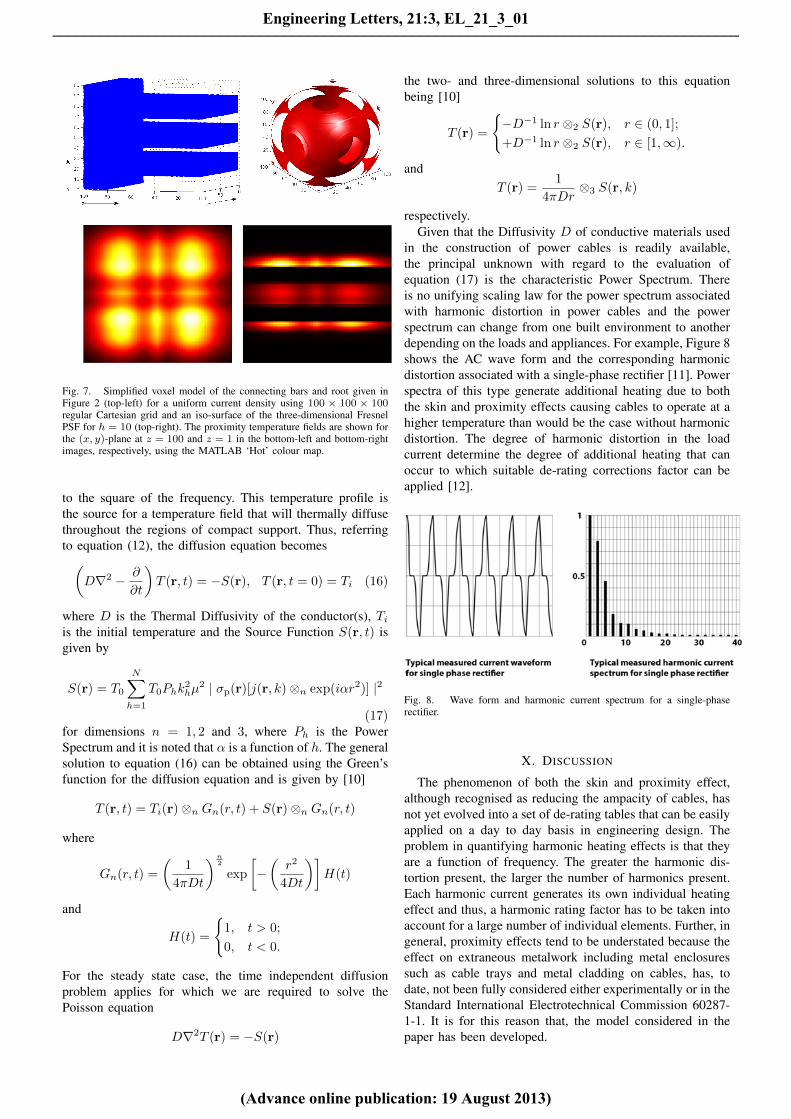
Fig. 7. Simplified voxel model of the connecting bars and root given inFigure 2 (top-left) for a uniform current density using 100 × 100 × 100regular Cartesian grid and an iso-surface of the three-dimensional FresnelPSF for h = 10 (top-right). The proximity temperature fields are shown forthe (x, y)-plane at z = 100 and z = 1 in the bottom-left and bottom-rightimages, respectively, using the MATLAB ‘Hot’ colour map.

to the square of the frequency. This temperature profile isthe source for a temperature field that will thermally diffusethroughout the regions of compact support. Thus, referringto equation (12), the diffusion equation becomes(

D∇2 − ∂

∂t

)T (r, t) = −S(r), T (r, t = 0) = Ti (16)

where D is the Thermal Diffusivity of the conductor(s), Tiis the initial temperature and the Source Function S(r, t) isgiven by

S(r) = T0

N∑h=1

T0Phk2hµ

2 | σp(r)[j(r, k)⊗n exp(iαr2)] |2

(17)for dimensions n = 1, 2 and 3, where Ph is the PowerSpectrum and it is noted that α is a function of h. The generalsolution to equation (16) can be obtained using the Green’sfunction for the diffusion equation and is given by [10]

T (r, t) = Ti(r)⊗n Gn(r, t) + S(r)⊗n Gn(r, t)

where

Gn(r, t) =

(1

4πDt

)n2

exp

[−(r2

4Dt

)]H(t)

and

H(t) =

{1, t > 0;

0, t < 0.

For the steady state case, the time independent diffusionproblem applies for which we are required to solve thePoisson equation

D∇2T (r) = −S(r)

the two- and three-dimensional solutions to this equationbeing [10]

T (r) =

{−D−1 ln r ⊗2 S(r), r ∈ (0, 1];

+D−1 ln r ⊗2 S(r), r ∈ [1,∞).

andT (r) =

1

4πDr⊗3 S(r, k)

respectively.Given that the Diffusivity D of conductive materials used

in the construction of power cables is readily available,the principal unknown with regard to the evaluation ofequation (17) is the characteristic Power Spectrum. Thereis no unifying scaling law for the power spectrum associatedwith harmonic distortion in power cables and the powerspectrum can change from one built environment to anotherdepending on the loads and appliances. For example, Figure 8shows the AC wave form and the corresponding harmonicdistortion associated with a single-phase rectifier [11]. Powerspectra of this type generate additional heating due to boththe skin and proximity effects causing cables to operate at ahigher temperature than would be the case without harmonicdistortion. The degree of harmonic distortion in the loadcurrent determine the degree of additional heating that canoccur to which suitable de-rating corrections factor can beapplied [12].

Fig. 8. Wave form and harmonic current spectrum for a single-phaserectifier.

X. DISCUSSION

The phenomenon of both the skin and proximity effect,although recognised as reducing the ampacity of cables, hasnot yet evolved into a set of de-rating tables that can be easilyapplied on a day to day basis in engineering design. Theproblem in quantifying harmonic heating effects is that theyare a function of frequency. The greater the harmonic dis-tortion present, the larger the number of harmonics present.Each harmonic current generates its own individual heatingeffect and thus, a harmonic rating factor has to be taken intoaccount for a large number of individual elements. Further, ingeneral, proximity effects tend to be understated because theeffect on extraneous metalwork including metal enclosuressuch as cable trays and metal cladding on cables, has, todate, not been fully considered either experimentally or in theStandard International Electrotechnical Commission 60287-1-1. It is for this reason that, the model considered in thepaper has been developed.



______________________________________________________________________________________

XI. CONCLUSIONS

The model developed in this paper is based on decou-pling Maxwell’s equations through application of a Gaugetransformation as detailed in Appendix A. The method ofsolution is based on a Green’s function solution for theMagnetic Vector Potential given the current density and theapplication of Ohm’s law. Under this condition the chargedensity is zero and application of the homogenous boundaryconditions on the surface of a conductor allows equation(11) is derived which shows that the proximity temperatureis proportional to the square frequency. With regard to thedevelopment of a proximity temperature simulation, the keyto the approach taken is to consider the Green’s functionsolution in the Fresnel zone which yields a convolution basedmodel compounded in equation (12).

The simulations are similar in both two- and three-dimensions and in both cases can be used to investigate theproximity heating effects generated at different harmonics.Higher harmonic effects are particularly important in thedesign of cable arrays and component structures but relieson knowledge of the spectrum of the harmonic componentspresent in the wave form of an AC load current which mustbe determined experimentally, a priori. Note that in theexample simulations presented, the primary current densityj is taken to be uniformly distributed which, in general, willnot be the case due to (self-induced) skin effects in the pri-mary conductor(s). Furthermore, the proximity conductivityσp may be non-uniform and the magnetic permeability µmay also be expected to change for different elements ofa power cable and proximity components. However, withinthe context of the model presented, these physical aspectsare readily incorporated.

One of the goals of the simulator developed is to evaluatethe possible presence of ‘hotspots’ in the design of cableconfigurations and proximal structures for harmonics that arepresent in the load. Although proximity temperature effectsare subject to thermal diffusion, as discussed in Section IX,in the context of the problem considered here, proximityrelated hotspots represent a continuous source of heat andcan therefore be evaluated independently of thermal diffusionprocesses. As these effects are also present in electricalmachines and equipment used in the built environment, inaddition to determining harmonic de-rating factors for powercables arranged in different layouts and combinations, thesimulator will provide a powerful design tool for a diverserange electrical equipment and machines which contain non-trivial conductor topologies and magnetic circuits.

APPENDIX A: MAXWELL’S EQUATIONS AND THEMAGNETIC VECTOR POTENTIAL

The motions of electrons (and other charged particles)give rise to electric and magnetic fields [13], [14]. Thesefields are described by the following equations which area complete mathematical descriptions for the physical lawsstated for constant electric permittivity ε and (constant)magnetic permeability µ.

Coulomb’s law∇ ·E =

ρ

ε(A.1)

Faraday’s law of induction

∇×E = −µ∂B∂t

(A.2)

No free magnetic monopoles exist

∇ ·B = 0 (A.3)

Modified (by Maxwell) Ampere’s law

∇×B = ε∂E

∂t+ j (A.4)

where E is the electric field, B is the magnetic field, jis the current density and ρ is the charge density Theseequations are used to predict the electric E and magneticB fields given the charge and current densities (ρ andj respectively) for the case when the material parametersdefined by ε and µ are constant. The differential operator ∇is defined as follows:

∇ ≡ i∂

∂x+ j

∂

∂y+ k

∂

∂z

for unit vectors (i, j, k). By including a modification toAmpere’s law, i.e. the inclusion of the ‘displacement current’term µ∂E/∂t, Maxwell provided a unification of electricityand magnetism compounded in the equations above.

A.1 Linearity of Maxwell’s Equations

Maxwell’s equations are linear because if

ρ1, j1 → E1, B1

andρ2, j2 → E2, B2

then

ρ1 + ρ2, j1 + j2 → E1 + E2, B1 + B2

where → means ‘produces’. This is because the operators∇·, ∇× and the time derivatives are all linear operators.

A.2 Solution to Maxwell’s Equations

The solution to these equations is based on exploitingthe properties of vector calculus and, in particular, identitiesinvolving the curl. Taking the curl of equation (A.2), we have

∇×∇×E = −µ∇× ∂B

∂t

and using the identity

∇×∇×E = ∇(∇ ·E)−∇2E

together with equations (A.1) and (A.4), we get

1

ε∇ρ−∇2E = −µ ∂

∂t

(ε∂E

∂t+ j

)or, after rearranging,

∇2E− 1

c2∂2E

∂t2=

1

ε∇ρ+ µ

∂j

∂t. (A.5)



______________________________________________________________________________________

wherec =

1√εµ

Taking the curl of equation (A.4), using the identity above,equations (A.2) and (A.3) and rearranging the result gives

∇2B− 1

c2∂2B

∂t2= −∇× j. (A.6)

Equations (A.5) and (A.6) are inhomogeneous wave equa-tions for E and B. These equations are ‘coupled’ to thevector field j (which is related to B). If we define a regionof free space where ρ = 0 and j = 0, then both E and Bsatisfy the equation

∇2f − 1

c2∂2f

∂t2= 0.

This is the homogeneous wave equation. One possible solu-tion of this equation (in Cartesian coordinates) is

fx = p(z − ct); fy = 0, fz = 0

which describes a wave or distribution p moving alongz at velocity c. Thus, in free space, Maxwell’s equationsdescribe the propagation of an electric and magnetic (orelectromagnetic field) in terms of a wave traveling at thespeed of light.

A.3 General Solution to Maxwell’s Equations

The solution to Maxwell’s equation in free space is specificto the charge density and current density being zero. We nowinvestigate a method of solution for the general case [15],[16]. The basic method of solving Maxwell’s equations (i.e.finding E and B given ρ and j) involves the following:

1) Expressing E and B in terms of two other fields Uand A.

2) Obtaining two separate equations for U and A.3) Solving these equations for U and A from which E

and B can then be computed.For any vector field A

∇ · ∇ ×A = 0.

Hence, if we writeB = ∇×A (A.7)

then equation (A.3) remains unchanged. Equation (A.2) canthen be written as

∇×E = −µ ∂∂t∇×A

or

∇×(E + µ

∂A

∂t

)= 0.

The field A is called the Magnetic Vector Potential. For anyscalar field U

∇×∇U = 0

and thus equation (A.2) is satisfied if we write

±∇U = E + µ∂A

∂tor

E = −∇U − µ∂A∂t

(A.8)

where the minus sign is taken by convention. U is called theElectric Scalar Potential.

Substituting equation (A.8) into Maxwell’s equation (A.1)gives

∇ ·(∇U + µ

∂A

∂t

)= −ρ

ε

or∇2U + µ

∂

∂t∇ ·A = −ρ

ε. (A.9)

Substituting equations (A.7) and (A.8) into Maxwell’s equa-tion (A.4) gives

∇×∇×A + ε∂

∂t

(∇U + µ

∂A

∂t

)= j

Finally, using the identity

∇×∇×A = ∇(∇ ·A)−∇2A

we can write

∇2A− 1

c2∂2A

∂t2−∇

(∇ ·A + ε

∂U

∂t

)= −j (A.10)

If we could solve equations (A.9) and (A.10) above for Uand A then E and B could be computed. The problem here,is that equations (A.9) and (A.10) are coupled. They canbe decoupled by applying a technique known as a ‘GaugeTransformation’. The idea is based on noting that equations(A.7) and (A.8) are unchanged if we let

A→ A +∇X

andU → U − ε∂X

∂tsince ∇ × ∇X = 0. If this gauge function X is taken tosatisfy the homogeneous wave equation

∇2X − 1

c2∂2X

∂t2= 0

then∇ ·A + ε

∂U

∂t= 0 (A.11)

which is called the Lorentz condition. With equation (A.11),equations (A.9) and (A.10) become

∇2U − 1

c2∂2U

∂t2= −ρ

ε(A.12)

and∇2A− 1

c2∂2A

∂t2= −j (A.13)

respectively. These equations are non-coupled inhomoge-neous wave equations and in this paper, the principal equa-tion used to derive a simulation for proximity effects isequation (A.13) with equation (A.8) serving to relate thesolution for A, via the Green’s function solution to equation(A.13), to the Electric Field E, subject to the conditionsthat ρ = 0 (appropriate for highly conductive media) andU = 0 (a consequence of using the homogeneous boundaryconditions).

ACKNOWLEDGMENTS

Jonathan Blackledge is supported by the Science Founda-tion Ireland Stokes Professorship Programme. The authorsacknowledge the support of the School of Electrical andElectronic Engineering at Dublin Institute of Technology,and, in particular, Dr Marek Rabow and Mr Derek Kearney.



______________________________________________________________________________________

REFERENCES

[1] Cenelec, ‘BS EN 50160:2000’, in Voltage Characteristics of ElectricitySupplied by Public Distribution Systems, 2000.

[2] Canelec, ‘BS EN 61000-3-2 Ed.2:2001 IEC 61000-3-2 Ed.2:2000Electromagnetic Compatibility (EMC)’, in Part 3-2: Limits for Har-monic Current Emissions (Equipment Input Current upto and Including16 A per Phase), 2001.

[3] IEEE, ‘IEEE Std 519-1992 (USA)’, IEEE Recommended Practicesand Requirements for Harmonic Control in Electrical Power Systems’,1992.

[4] N. R. W. J. Arrillaga, Power System Harmonics, Second Edition ed.:John Wiley and Sons, Ltd, 2003.

[5] S. J. B. Ong and C. YeongJia, An Overview of International HarmonicsStandards and Guidelines (IEEE, IEC, EN, ER and STC) for LowVoltage System, Power Engineering Conference, IPEC (2007), 602-607, 2007.

[6] Voxelogic, http://www.voxelogic.com[7] Voxel Sculpturing http://3d-coat.com/voxel-sculpting/[8] VoxCad, http://www.voxcad.com/[9] Pendix, http://home.arcor.de/sercan-san/homepage/sangames/sites/

project pendix.html[10] G. A. Evans, J. M. Blackledge and P. Yardley, Analytical Solutions to

Partial Differential Equations, Springer, 1999.[11] Gambica (Ed.), Managing Harmonics: A Guide to ENA Engineering

Recommendation G5/4-1, Sixth Edition, 2011.[12] K. O’Connell, J. M. Blackledge, M. Barrett and A. Sung, Cable

Heating Effects due to Harmonic Distortion in Electrical Installations,International Conference of Electrical Engineering, World Congress onEngineering (WCE2012), London 4-6 July, IAENG, 928-933, 2012.

[13] J. A. Stratton, Electromagnetic Thoery, McGraw-Hill, 1941.[14] P. M. Morse and H. Feshbach, Methods of Theoretical Physics,

McGraw-Hill, 1953.[15] R. H. Atkin, Theoretical Electromagnetism, Heinemann, 1962.[16] B. I. Bleaney, Electricity and Magnetism, Oxford University Press,

1976.

Professor Jonathan Blackledge holds a PhD in The-oretical Physics from London University and a PhD inMathematical Information Technology from the Univer-sity of Jyvaskyla. He has published over 200 scientificand engineering research papers including 14 books, has

filed 15 patents and has been supervisor to over 200 MSc/MPhil and PhDresearch graduates. He is the Science Foundation Ireland Stokes Professorat Dublin Institute of Technology where he is also an Honorary Professorand Distinguished Professor at Warsaw University of Technology. He holdsFellowships with leading Institutes and Societies in the UK and Irelandincluding the Institute of Physics, the Institute of Mathematics and itsApplications, the Institution of Engineering and Technology, the BritishComputer Society, the Royal Statistical Society and Engineers Ireland.

Professor Eugene Coyle is Head of Research Innovationand Partnerships at the Dublin Institute of Technology.His research spans the fields of control systems andelectrical engineering, renewable energy, digital signalprocessing and ICT, and engineering education and haspublished in excess of 120 peer reviewed conference and

journal papers in addition to a number of book chapters. He is a Fellowof the Institution of Engineering and Technology, Engineers Ireland, theEnergy Institute and the Chartered Institute of Building Services Engineers,was nominated to chair the Institution of Engineering and Technology (IET)Irish branch committee for 2009/10 and a member, by invitation, of theEngineering Advisory Committee to the Frontiers Engineering and ScienceDirectorate of Science Foundation Ireland, SFI.

Kevin O’Connell was previously Head of the Depart-ment of Electrical Services Engineering until his retire-ment in September 2010 and now a PhD student at DublinInstitute of Technology working with Professor JonathanBlackledge and Professor Eugene Coyle. He recentlyobtained the Best Paper Award for his paper entitled

Cable Heating Effects due to Harmonic Distortion in Electrical Installations,with co-authors, Martin Barrett, Jonathan Blackledge and Anthony Sung.The paper was presented at the International Conference on Electronicsand Electrical Engineering at the The World Congress on Engineering 2012(WCE2012) held at Imperial College, London in July 4-6, 2012.



______________________________________________________________________________________

proximity heating effects in power cables · proximity heating effects in power cables jonathan...

Documents