proving tight bounds on univariate expressions with ...melquion/doc/15-jar.pdfproving tight bounds...

JAR manuscript No.(will be inserted by the editor)

Proving Tight Bounds on Univariate Expressions withElementary Functions in Coq

Érik Martin-Dorel · Guillaume Melquiond

Received: date / Accepted: date

Abstract The verification of floating-point mathematical libraries requires computing nu-merical bounds on approximation errors. Due to the tightness of these bounds and the pecu-liar structure of approximation errors, such a verification is out of the reach of generic toolssuch as computer algebra systems. In fact, the inherent difficulty of computing such boundsoften mandates a formal proof of them. In this paper, we present a tactic for the Coq proofassistant that is designed to automatically and formally prove bounds on univariate expres-sions. It is based on a formalization of floating-point and interval arithmetic, associated withan on-the-fly computation of Taylor expansions. All the computations are performed insideCoq’s logic, in a reflexive setting. This paper also compares our tactic with various existingtools on a large set of examples.

Keywords Interval arithmetic · Formal proof · Decision procedure · Coq proof assistant ·Floating-point arithmetic · Nonlinear arithmetic

1 Introduction

Libraries of mathematical functions (so called libm) are pieces of software that providefloating-point approximations of the most common mathematical functions, e.g. exp, cos.The use of such functions is so pervasive nowadays that the IEEE 754–2008 standard forfloating-point arithmetic gives recommendation on their accuracy. As such, it is critical thatlibraries document the accuracy of the computed values, so that users of those librariescan rely on them. In fact, some library authors go as far as publishing mathematical proofsshowing that the documented accuracy is correct.

This work was funded by the Verasco ANR project (ref. ANR-11-INSE-003). It was partly done while thefirst author was with Inria Saclay–Île-de-France, in the LRI research laboratory.

Érik Martin-DorelUniversité Toulouse 3–Paul Sabatier, Institut de Recherche en Informatique de Toulouse, UMR 5505 CNRSIRIT, Université Paul Sabatier, 118 route de Narbonne, 31062 Toulouse Cedex 9, France

Guillaume MelquiondInria Saclay–Île-de-France, LRI, UMR 8623 CNRSPCRI, bât 650, Université Paris-Sud, F-91405 Orsay Cedex, France

2 Érik Martin-Dorel, Guillaume Melquiond

For instance, if we take a look at the correctness proof for the implementation of exp inthe CRlibm library,1 we can notice that it relies on the following assumption, among others:For any x such that |x | ≤ 355 · 2−22, we have the following bound:

��x + 0.5 · x2 + c3x3 + c4x4 − exp x + 1

exp x − 1

��≤ 2−62 (1)

with c3 = 6004799504235417 · 2−55 and c4 = 1501199876148417 · 2−55.Verifying such an assumption by hand is extremely tedious and error-prone. So we might

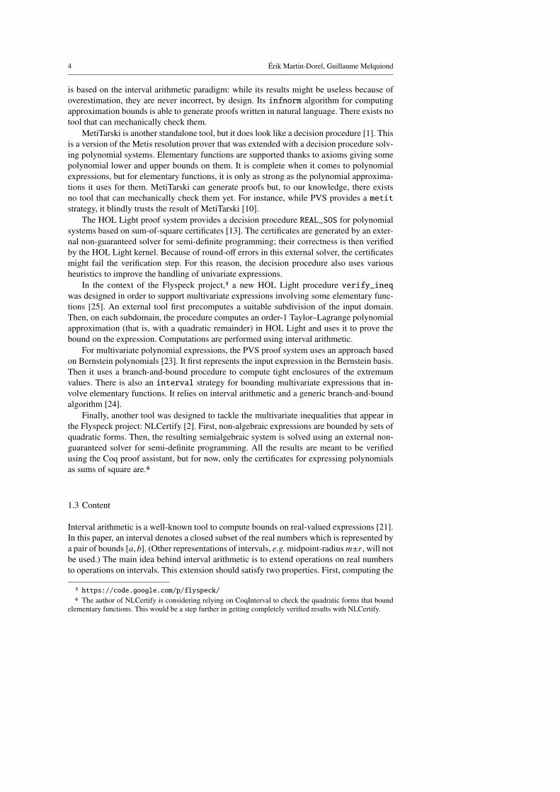
first want to get a bit more insight on that property. Since the relative error it bounds isa well-behaved univariate function of x, we could first try to plot it with some computeralgebra system: Maple, Mathematica, Matlab, and so on. Indeed, if the extremum points ofthe function graph visually satisfy the property, then the assumption is most probably valid.While not a formal proof in any way, this check would already go a long way in increasingthe confidence in the library. Unfortunately, as can be seen on Figure 1, the resulting plotlooks so fishy that it might have the opposite effect on the users: a decreased confidencein the library. The reason why standard tools such as Gnuplot fail to plot the relative errorof this function should not come as a surprise. Indeed, their plotting procedures performbinary642 computations, as it is the floating-point arithmetic natively supported by mostprocessors. Such computations have a precision of 53 bits, while the relative error we areinterested in is 2−62. For instance, a precision of at least 90 bits is needed for the plot to looksensible when using Sage.

-5e-12

0

5e-12

1e-11

1.5e-11

2e-11

-8e-05 -6e-05 -4e-05 -2e-05 0 2e-05 4e-05 6e-05 8e-05

-2.5e-19

-2e-19

-1.5e-19

-1e-19

-5e-20

0

5e-20

-8e-05 -6e-05 -4e-05 -2e-05 0 2e-05 4e-05 6e-05 8e-05

Fig. 1 On the left, the function from Equation (1), as plotted by the Gnuplot tool, which relies on binary64floating-point numbers. On the right, its actual graph, as plotted by Sollya.4

At that point, we have no other choice than to turn to some other tools, if we everwant to trust the correctness proofs of mathematical libraries. The property above is quiterepresentative of the kind of statements one encounters when proving a mathematical library.In fact, the correctness of a modern library might depend on the proof of hundreds of tightbounds on univariate functions, for table-based implementations [22]. Ideally, we shouldeven go all the way to a formal proof, to get the highest confidence in the implementation ofthese libraries.

1 http://lipforge.ens-lyon.fr/www/crlibm/

2 Binary64 is the name of the IEEE 754–2008 floating-point format that was formerly known as the “dou-ble precision” format.4 http://sollya.gforge.inria.fr/

http://lipforge.ens-lyon.fr/www/crlibm/

http://sollya.gforge.inria.fr/

Proving Tight Bounds on Univariate Expressions with Elementary Functions in Coq 3

1.1 Background and Scope

Historically, the CoqInterval development was at the origin of this effort to verify boundson univariate functions by using the Coq proof assistant. It provided a formalization of acomputable floating-point library [18] and a decision procedure based on interval arithmeticwas built on top of it [19]. The floating-point reference algorithms were later moved to theFlocq library [3], while the CoqInterval library focused on formalizing faster versions of thefloating-point operators and elementary functions [20]. Independently developed, the Coq-Approx library was built on top of CoqInterval’s formalization of interval arithmetic. It wasdesigned to compute formally-verified polynomial approximations of univariate functionswhich can then be fed to programs solving the Table-Maker’s Dilemma [4,17].

So, at that point in time, we had, on one side, a decision procedure to verify bounds onunivariate functions and, on the other side, a library able to generate accurate polynomialapproximations. Since verifying bounds on a univariate polynomial might be faster thanon an arbitrary function, it was then natural to try to merge both approaches in order toget a more efficient decision procedure for the Coq proof assistant. This paper gives anoverview of how these different libraries are combined together and what features they offerin the context of automatically and formally verifying bounds on univariate functions. Theresulting decision procedure is part of the CoqInterval formalization, which is available at

http://coq-interval.gforge.inria.fr/

Before going any further, let us describe which kind of expressions we intend to provebounds on. At first, we can qualify these expressions as being univariate: only one variablecan occur in them; all the other arity-0 symbols are numeric constants. This is a bit toorestrictive though. Indeed, the approach we present is based on interval arithmetic, so theamount of variables does not really matter, only the number of their occurrences does. Abetter description would therefore be that, for tight bounds to be computed, among all thevariables of the expression, only one (say, x1) occurs several times. In the sequel, we will saythat such an expression is quasi-multivariate. Note that this requirement could be relaxeda bit further: if a variable is the only one to appear in a sub-expression, it can be seenas appearing only once in that sub-expression. For instance, the function f (x, y) = x +

cos(x + (y + exp(y))) fits this interpretation since y only occurs in the (y + exp(y)) sub-expression and x does not occur there. As a consequence, the methods presented in this papercould deal with such a function. Still this hardly covers all the multivariate expressions,hence the usage of “univariate” and “quasi-multivariate” to characterize the expressions theCoqInterval library can handle.

1.2 Related Works

There are various other systems that make it possible to prove inequalities on real-valuedexpressions. Their purposes are rather diverse. Some are limited to univariate expressions,while others can deal with multivariate expressions. Some are limited to polynomial ex-pressions, while others also support some elementary functions, e.g. exp, tan. Finally, somegenerate proofs that are mechanically checked by proof assistants, while others are stan-dalone tools.

Let us start with Sollya [7,6]. Its interface looks like it comes from a generic computeralgebra system but the tool is dedicated to manipulating univariate expressions and com-puting guaranteed bounds on them. It supports a large range of elementary functions. It

http://coq-interval.gforge.inria.fr/


is based on the interval arithmetic paradigm: while its results might be useless because ofoverestimation, they are never incorrect, by design. Its infnorm algorithm for computingapproximation bounds is able to generate proofs written in natural language. There exists notool that can mechanically check them.

MetiTarski is another standalone tool, but it does look like a decision procedure [1]. Thisis a version of the Metis resolution prover that was extended with a decision procedure solv-ing polynomial systems. Elementary functions are supported thanks to axioms giving somepolynomial lower and upper bounds on them. It is complete when it comes to polynomialexpressions, but for elementary functions, it is only as strong as the polynomial approxima-tions it uses for them. MetiTarski can generate proofs but, to our knowledge, there existsno tool that can mechanically check them yet. For instance, while PVS provides a metitstrategy, it blindly trusts the result of MetiTarski [10].

The HOL Light proof system provides a decision procedure REAL_SOS for polynomialsystems based on sum-of-square certificates [13]. The certificates are generated by an exter-nal non-guaranteed solver for semi-definite programming; their correctness is then verifiedby the HOL Light kernel. Because of round-off errors in this external solver, the certificatesmight fail the verification step. For this reason, the decision procedure also uses variousheuristics to improve the handling of univariate expressions.

In the context of the Flyspeck project,5 a new HOL Light procedure verify_ineqwas designed in order to support multivariate expressions involving some elementary func-tions [25]. An external tool first precomputes a suitable subdivision of the input domain.Then, on each subdomain, the procedure computes an order-1 Taylor–Lagrange polynomialapproximation (that is, with a quadratic remainder) in HOL Light and uses it to prove thebound on the expression. Computations are performed using interval arithmetic.

For multivariate polynomial expressions, the PVS proof system uses an approach basedon Bernstein polynomials [23]. It first represents the input expression in the Bernstein basis.Then it uses a branch-and-bound procedure to compute tight enclosures of the extremumvalues. There is also an interval strategy for bounding multivariate expressions that in-volve elementary functions. It relies on interval arithmetic and a generic branch-and-boundalgorithm [24].

Finally, another tool was designed to tackle the multivariate inequalities that appear inthe Flyspeck project: NLCertify [2]. First, non-algebraic expressions are bounded by sets ofquadratic forms. Then, the resulting semialgebraic system is solved using an external non-guaranteed solver for semi-definite programming. All the results are meant to be verifiedusing the Coq proof assistant, but for now, only the certificates for expressing polynomialsas sums of square are.6

1.3 Content

Interval arithmetic is a well-known tool to compute bounds on real-valued expressions [21].In this paper, an interval denotes a closed subset of the real numbers which is represented bya pair of bounds [a,b]. (Other representations of intervals, e.g. midpoint-radius m±r , will notbe used.) The main idea behind interval arithmetic is to extend operations on real numbersto operations on intervals. This extension should satisfy two properties. First, computing the

5 https://code.google.com/p/flyspeck/

6 The author of NLCertify is considering relying on CoqInterval to check the quadratic forms that boundelementary functions. This would be a step further in getting completely verified results with NLCertify.

https://code.google.com/p/flyspeck/


result of an interval operator should only involve arithmetic operations on the bounds of theinput intervals, so that computing with intervals is both effective and efficient in practice.Second, the interval operators should satisfy the containment property: the resulting intervalshould be large enough so that it contains all the possible results of the operation appliedto real numbers. That way, interval arithmetic can be used to formally prove properties onreal-valued expressions. Section 2 gives some preliminaries about interval arithmetic andpresents the interval tactic for proving tight bounds on univariate and quasi-multivariateexpressions automatically. It also shows how the CoqInterval library is structured.

For the proofs to be performed automatically, the Coq proof assistant has to be able to ef-fectively compute using intervals. For that purpose, a floating-point arithmetic is formalizedin Coq and proved correct with respect to real arithmetic. Then an interval arithmetic is builtusing floating-point numbers as bounds and proved to preserve the containment property.Section 3 shows how these arithmetics are formalized in Coq.

Thanks to containment, properties that can be deduced from an interval computationare trivially correct. Unfortunately, interval arithmetic is plagued by a major issue calledthe dependency effect. Indeed, the efficiency of interval arithmetic does not come for free:while the resulting intervals are guaranteed to contain any possible real result, the overes-timation might be so coarse that it is impossible to deduce any non-trivial fact from them.The archetype of this situation is the interval (−∞,+∞), which trivially contains all possi-ble real values for the expression under study, but yields no further information. This issueappears as soon as a variable occurs several times in an expression evaluated by intervalcomputations. Indeed, naive interval arithmetic does not track the dependencies between allthese occurrences. Section 4 presents three approaches that we have formalized in Coq toalleviate this issue: bisection, automatic differentiation, and Taylor models.

Finally, Section 5 compares the performance of our implementation with all the toolsdescribed in Section 1.2 on a large set of examples. These examples contain various ap-proximation problems, but also some tests taken from MetiTarski, and some well-knownmultivariate problems.

2 The interval and interval_intro Tactics

The CoqInterval library provides two tactics that allow one to automatically perform proofsusing interval computations: interval and interval_intro. The interval tactic ap-plies to goals that are inequalities over the reals. If the tactic cannot solve the goal, it failswith an error message. The interval_intro tactic is useful when doing some forward rea-soning: when called on an expression, it computes an enclosure of it, then formally provesit using interval, and finally adds it to the proof context. The syntax of these two tacticsis as follows:

– interval [options],– interval_intro expr [mode] [options].

By default, interval_intro computes both a lower and an upper bound for expr. If onlyone of them is needed, one can tell the tactic about it by specifying lower or upper as amode, so as to speed up the proof process. Both tactics can be configured with the followingoptions:

– “i_prec p” changes the precision of floating-point computations (default: 30 bits),– “i_depth n” changes the maximum depth of the bisection process (default: 15 forinterval, 5 for interval_intro),


– “i_bisect x” asks for a bisection along variable x (Section 4.1),– “i_bisect_diff x” asks for a bisection and an automatic differentiation of expressions

with respect to variable x (Section 4.2),– “i_bisect_taylor x d” asks for a bisection and the computation of degree-d Taylor

models with respect to variable x (Section 4.3).Obviously, the last three options are mutually exclusive, and if none of them is passed, thetactic does not use any method to reduce the dependency effect.

Below is a toy example showing the usage of the tactic. (Rabs denotes the absolute valuein Coq; other symbols have their intuitive meaning.)

Goalforall x, 3/2 <= x <= 2 ->forall y, 1 <= y <= 33/32 ->Rabs (sqrt(1 + x / sqrt(x + y))

- 144/1000*x - 118/100) <= 71/32768.Proof.intros.interval with (i_prec 19, i_bisect x).

Qed.

Notice that the goal inequality involves two variables x and y. In fact, the tactic cancope with an arbitrary number of variables; but the methods for reducing the dependencyeffect can be applied to only one of those variables, here x. As for performance, the formalverification takes half a second, which is slow with respect to some other Coq tactics, butstill tolerable for the user.

The tactic supports any expression composed of the following standard Coq operators:Ropp (unary minus), Rabs (absolute value), Rinv (multiplicative inverse), Rsqr (square),sqrt, cos, sin, tan, atan, exp, ln, pow (power by a nonnegative integer), powerRZ (powerby any integer), Rplus, Rminus, Rmult, Rdiv. The constant PI is also supported. There aresome restrictions on the domain of a few functions: pow and powerRZ are only supportedif the exponent has a numeric value; inputs of cos and sin should be between −2π and2π; inputs of tan should be between −π/2 and π/2. If not, the tactic might fail to proveanything interesting. These restrictions on the trigonometric functions are related to the naiveimplementation of their interval versions; any improvement to their code would lift them.

2.1 Preliminaries About Interval Arithmetic

Throughout this article, a boldface variable x denotes an interval enclosing a real variable x.Its lower and upper bounds are written x and x, so that x = [x, x]. A function over realnumbers is denoted f and its application is f (x). The image of interval x by f is f (x); it isdefined as

f (x) = {y | ∃x ∈ x, y = f (x)} .An interval extension of f is denoted f. It is not uniquely defined, since it just has to satisfythe containment property:

∀x ⊆ R, f (x) ⊆ f(x).Interval operators usually satisfy some other properties, such as isotonicity,7 but they are notrequired to prove the correctness of the operator itself. As a matter of fact, the isotonicity

7 An interval function f is isotone if, for any pair of intervals (x, x′), we have x ⊆ x′ =⇒ f(x) ⊆ f(x′)(see also [11, Definition 4.8.10]).


property does not occur in any of our proofs, but it explains why the bisection technique(presented later on in the paper) can reduce the dependency effect.

The main idea behind interval arithmetic, dubbed the fundamental theorem of intervalanalysis, is that the containment property is preserved by function composition, e.g. f ◦ g isan interval extension of f ◦ g [21]. Thus one only needs to build interval extensions of basicoperators in order to perform interval computations.

In order to prove that the formula ∀x1 ∈ x1, . . . , ∀xn ∈ xn, f (x1, . . . , xn ) ∈ y holdsfor some composite expression f , one first builds an interval extension f of f using basicinterval extensions and composition. Then one computes f(x1, . . . ,xn) and checks whetherit is a subset of y. If it is a subset, the original formula holds. That is the way the tactic usesinterval arithmetic to automatically prove properties.

So as to support half-bounded intervals, we allow x to be −∞, and x to be +∞. (Notethat, while we denote intervals with square brackets, in the case of infinite bounds, theyare not part of the interval, that is, [−∞,+∞] = R.) Infinite bounds are not a mandatoryfeature of interval arithmetic and one could define a usable one without them. It is helpful tohave them though, as we ultimately want to reason about inequalities, which half-boundedintervals make easy to represent. For instance, in order to prove that ∀x, x ≤ 0⇒ f (x) ≥ 0,one can just compute the following interval inclusion: f([−∞,0]) ⊆ [0,+∞].

Let us now consider the interval subtraction as an example. One way to define thisoperator sub so that it satisfies the containment property is as follows:

∀u,v ⊆ R, sub(u,v) = [u − v,u − v]. (2)

Notice that an interval subtraction can be performed at the cost of just two bound subtrac-tions, which makes it an efficient operation. Generally speaking, most interval operationshave this kind of complexity. The implementation is rather straightforward, though one hasto be careful when performing the operations on bounds, due to the potential presence ofinfinities. They also tend to make the proof of the containment property a bit cumbersomedue to the explosion of cases.

Let us consider another example, the exponential function. Due to the monotonicity ofexp, the containment property is trivially satisfied by the following interval extension:

∀u ⊆ R, exp(u) = [exp(u),exp(u)].

It raises a question though: how to represent bounds? As can be seen on that example,they can indeed be almost any real number. We could simply use standard real numbers torepresent them, but that would prevent us from using the reduction engine to perform com-putations on them, so this is not a suitable solution for a Coq implementation. We couldrestrict the bounds to computable real numbers instead, but we expect that such an imple-mentation would not be tractable, due to performance issues.

This issue is not new and was dealt with by every arithmetician wanting to effectivelycompute such interval extensions. Since the only property we are interested in is the con-tainment property, an interval result does not have to be the tightest possible one, it can beslightly enlarged. As a consequence, instead of real numbers, one can use any subset of Ras the set of finite bounds. We only need to have some functions 5 and 4 that, given a realnumber, return a bound that is smaller, respectively larger. The interval extension of exp canthen be defined as

∀u ⊆ R, exp(u) = [5(exp(u)),4(exp(u))]. (3)


Note that these two functions 5 and 4 are only for exposition and proof purpose. We cannotfirst compute the exponential and then round it to a bound. Both operations happen at once:given a bound b, we compute a bound that is smaller (resp. larger) than exp(b).

Now, which subset of real numbers to choose? We could use rational numbers as wasdone in PVS [8]. But numerators and denominators of rational numbers tend to grow duringcomputations, hence making them slower as they progress further. To prevent this growth,we could round rational numbers from time to time. But if we are to round them, we mightjust as well use only floating-point numbers (a subset of rational numbers) as they are espe-cially suited for rounded operations.

2.2 Architecture of CoqInterval

Our CoqInterval library has been designed with a special focus on modularity, in orderto easily switch the implementation of basic building blocks, but also to facilitate furtherextensions of the formalization. Its architecture is summarized in Figure 2.

The “Tactic” module provides the tactics themselves and their implementation: pars-ing the expressions and the bounds, creating a suitable formal proof, and causing Coq tocheck it automatically (see Section 2.3). It relies on several modules that are able to com-pute bounds of real-valued expressions. One of the approaches is based on automatic differ-entiation “Auto-diff” (see Section 4.2). Another approach is based on rigorous polynomialapproximations using “Taylor models” (see Section 4.3); they are built using the CoqApproxlibrary [4,17], now part of CoqInterval.

Both approaches perform interval computations and can be parameterized by any imple-mentation of interval arithmetic that satisfies the “IntervalOps” interface. The CoqIntervallibrary comes with one such implementation: “FloatInterval” (see Sections 3.2 and 3.3). Itrepresents intervals as pairs of floating-point bounds. Again, the implementation of floating-point arithmetic is not fixed and any implementation that satisfies the “FloatOps” interfacecan be used to obtain an interval arithmetic. This interface provides basic arithmetic opera-tors such as +, ×,

√· (see Section 3.1).

Finally, several implementations provide a floating-point arithmetic satisfying “FloatOps”.All these implementations are proved correct using a reference implementation based on theFlocq library [3]. The simplest implementation, “GenericFloat”, just reflects the referenceimplementation. The other implementation, “SpecificFloat”, provides optimized versions ofthe operators, given some dedicated operations on integers. These dedicated operations aredescribed by the “FloatCarrier” interface. Two radix-2 implementations of this interface areprovided “StdZRadix2” and “BigIntRadix2”. The differences between these two implemen-tations are the performance and the surface of the Coq kernel they exercise. “BigIntRadix2”is the fastest one, while “StdZRadix2” uses a smaller part of the kernel.

To summarize, the tactics rely on the following modules. They use the “Auto-diff” and“Taylor models” modules to perform bound computations. The tactics instantiate these mod-ules using an interval arithmetic provided by the “FloatInterval” module, which they instan-tiate using the “SpecificFloat” implementation of floating-point arithmetic. Finally, the tac-tics instantiate this last module using “BigIntRadix2” which provides a fast arithmetic overradix-2 integers.


Flocq

CoqInterval

CoqApprox

FP reference impl.

«interface»FloatOps

radix : {β : Z | β ≥ 2}F : Typezero : F

add(mode, prec) : F→ F→ F

GenericFloatSpecificFloat

«interface»FloatCarrier

radix : {β : Z | β ≥ 2}

...

«interface»IntervalOps

I : Typezero : I

add(prec) : I→ I→ Iexp(prec) : I→ I

StdZRadix2 BigIntRadix2

FloatInterval

Auto-diff. Taylor models

Tactic

interval [options]interval_intro expr [mode] [options]

Fig. 2 Diagram (UML) that summarizes the architecture of the CoqInterval package.The three kinds of arrows involved in the figure are:A I if the module A is parameterized by a module that implements the interface I,C I if the module C implements the interface I,M C if the module M uses the module C.

2.3 Reification and Reflection

The interval tactic works by reflection. Given a goal G to prove, it constructs a Booleanexpression b, such that the following implication holds:

b = true⇒ G.

This general theorem has been proved once and for all; Coq just has to check that b andG are suitable to instantiate it. Once this theorem has been applied to the goal, what is leftto prove is just b = true. Then the tactic tells Coq that this is just a consequence of the


reflexivity of equality. The formal checker of Coq is thus forced to evaluate b to verify thatit is indeed equal to true (assuming the goal was provable this way), which concludes theproof. In the context of Coq, this approach has two advantages. First, it leverages the efficientreduction engines for the evaluation of b. Second, it produces proof terms that are tiny: justtwo deduction steps.

An important point about reflection is that b is not a small expression. Indeed, severallibraries about integer arithmetic, a library about lists, a library about floating-point arith-metic, a library about interval arithmetic, a library about Taylor models, etc., were used todesign the interval tactic. All the computable parts of these libraries might end up in b,depending on which options were passed to the tactic. In fact, if the definitions were to beunfolded, b would amount to several hundreds of lines of ML code. So it should not comeas a surprise that the evaluation of b is the expensive stage of the verification process.

Naive interval arithmetic, automatic differentiation, and Taylor models all follow thesame approach: they inductively perform computations on the sub-expressions in order todeduce the range of the whole expression. Therefore, to automate this process, we need aninductive representation of expressions. An abstract syntax tree would work, but we wantedto allow for some sharing between common sub-expressions, so as to avoid performingthe same computations several times. So, instead, we represent expressions as straight-lineprograms with static single assignment. An expression is a sequence of statements, eachstatement being composed of an arithmetic operator and some integers pointing to the loca-tion of the inputs. For instance, the expression (x + y) · x + (x + y) is reified into the followingprogram, with comments indicating which values would be contained in the program stackbefore evaluating each statement.

(* initial state: [y, x] *) Binary Add 1 0(* current state: [x+y, y, x] *) :: Binary Mul 0 2(* current state: [(x+y)*x, x+y, y, x] *) :: Binary Add 0 1(* current state: [(x+y)*x+(x+y), ...] *) :: nil

We have designed a generic evaluator for such programs. The tactic instantiates it inseveral different ways to prove the goal. First, there is a trivial instance that associates toeach operator the corresponding uninterpreted function on real numbers. Given a program,the evaluator thus produces the original real-valued expression; it is used to check that thereification process produced the correct program. Then, there are three specializations of theevaluator to do actual computations, one with single intervals, one with pairs of intervalsfor automatic differentiation, and one with sequences of intervals for Taylor models. Forthese three instances, we have proved that the arithmetic operators satisfy the respectivecontainment properties, and by induction, that the program evaluations do, too.

3 Arithmetic Computations Inside Coq

The CoqInterval library defines an interval type with bounds represented by floating-pointnumbers. It provides several arithmetic operators over intervals and proves that they respectthe containment property. The implementation of these operators relies on performing com-putations on interval bounds using floating-point operators. Section 3.1 gives an overviewof how these floating-point operators for addition, multiplication, division, and square root,are defined. Section 3.2 then presents the interval type and how to define interval operatorsfor addition, multiplication, and so on. Finally, Section 3.3 shows how to combine basic


floating-point and interval operators to compute floating-point approximations and intervalextensions of elementary functions, e.g. exp and cos.

3.1 Floating-point Operators

Floating-point numbers are rational numbers that can be written m · βe with m and e twointegers and β a fixed integer larger than or equal to 2. The CoqInterval library does notprovide any mixed-radix operation, so let us assume that β is fixed once and for all. The setof floating-point numbers is

F ={x ∈ R �� ∃m,e ∈ Z, x = m · βe } .

Note that the representation of a real number as a floating-point number m·βe , if it exists,is not unique. In practice, this is neither an issue nor a source of inefficiency (floating-pointrounding prevents the integers from growing large, as seen below), so we do not have torestrict m to integers that are not multiple of β.

Defining addition and multiplication on this representation is straightforward:

(m1 · βe1 ) + (m2 · βe2 ) = (m1 × βe1−e + m2 × βe2−e ) · βe with e = min(e1,e2),

(m1 · βe1 ) × (m2 · βe2 ) = (m1 × m2) · βe1+e2 . (4)

Obviously, such operations suffer from the same growth that caused us to discard rationalnumbers in the first place. So let us introduce the operators 5 and 4. These operators areparameterized by a precision p. This positive integer specifies how many radix-β digitsthe resulting mantissa can have at most. Contrarily to β, the value of p can be selected ona per-operation basis. As a matter of fact, the CoqInterval library increases the precisionof intermediate computations on-the-fly when approximating elementary functions, if thecurrent precision would lead to grossly inaccurate results; this will be detailed in Section 3.3.

To define 5 and 4, let us first restrict F to the following subset:

Fp ={m · βe ∈ F �� |m | < βp

}which will be the range of these operators. They can now be defined as

5(x) = max{y ∈ Fp

�� y ≤ x}

and 4(x) = min{y ∈ Fp

�� y ≥ x}. (5)

By definition, we have 5(x) ≤ x ≤ 4(x) for any real x. So these operators are sufficient toensure the containment property. The definitions of F, of Fp , and of the rounding operatorscome from the Flocq library, a multi-radix multi-precision multi-format formalization offloating-point arithmetic in Coq [3].

Notice that these operators return the tightest representable enclosure of x, which ismuch stricter than what is actually needed for automated proof purpose. Their definitions,however, make it possible to use external tools to test the Coq implementation, and vice-versa. Indeed, these definitions comply with the IEEE-754 standard for floating-point arith-metic and are thus found in most floating-point hardware and in libraries such as SoftFloat8or MPFR.9 Note that the precision p is arbitrary for MPFR, while it is restricted to a few val-ues (e.g., p = 24 and p = 53) for hardware and SoftFloat. A peculiarity of the floating-point

8 http://www.jhauser.us/arithmetic/SoftFloat.html

9 http://www.mpfr.org/

http://www.jhauser.us/arithmetic/SoftFloat.html

http://www.mpfr.org/


formalization of CoqInterval is that the exponent range of the numbers in Fp is unbounded,implying that no arithmetic underflow nor overflow can occur.

The definitions of 5 and 4 in Equation (5) are suitable for proofs, but they do not offera way to actually compute the results of the operators. So they are not amenable to auto-mated proof. So the CoqInterval library also provides some functions that, given a value ofF compute a value of Fp . For instance, Fround_at_prec(β,mode,p,m · βe ) returns theelement of Fp the closest to m · βe , with the meaning of closest being controlled by mode(5 or 4). Then one can just compose such a function with + and × to get rounded values.For instance, the rounded multiplication between two floating-point values is defined in ourCoqInterval library as follows.

Definition Fmul beta mode prec (x y : float beta) :=Fround_at_prec mode prec (Fmul_aux x y).

In this definition, Fmul_aux is the exact product between two floating-point numbers of typeFβ , as defined in Equation (4).

For division and square root, however, this approach does not work, since the interme-diate results cannot be represented as values of F. So dedicated algorithms are provided forthese operators. While originally designed for the CoqInterval library, these algorithms andtheir proofs have now migrated to Flocq.

That said, even if the algorithms in Flocq are useful as reference implementation, theyhave not been implemented with a strong concern about performance. In particular, they donot take advantage of the value of β or of the regularity of Fp (fixed precision, no subnormalnumbers). So our library also provides some optimized versions of these algorithms, whichare proved equivalent to the ones in Flocq. For instance, when integers use a radix-β rep-resentation, to know whether an integer is a multiple of βk , rather than performing a costlyEuclidean division, one can just count the number of less-significant digits that are equal tozero.

In the end, our CoqInterval library proposes several implementations of the basic floating-point operators. For instance, one uses the Z type of integers represented as a string of bits,while another one uses the BigZ type of integers represented as a balanced binary tree of31-bit native integers. All these implementations have the same interface though (see Fig-ure 2), so the user can swap one for the other. In particular, the interval operators (presentedin Section 3.2) do not care about the actual implementation of the floating-point operators.

In our setting, the floating-point formalization just has to provide an implementation ofthe following floating-point operations and their correctness proofs: comparison, minimum,maximum, absolute value, opposite, exact addition, exact subtraction, exact multiplication,addition, subtraction, multiplication, division, square root, multiplication by a power of β,multiplication by a power of 2, rounding, conversion from Z, and so on. The complete in-terface can be found in the Interval_float_sig.v file. From now on, F will denote anoptimized implementation of this interface. So, while Fmul is a reference floating-pointmultiplication using non-optimized integer computations, F.mul provides an optimized im-plementation for a fixed radix β.

One last point about our floating-point arithmetic is that it supports a ⊥ element that ispropagated along the computations. So, the domain of all the functions is not F but F = F∪{⊥}, and floating-point operations are extended accordingly, so ⊥ is an absorbing element.Note that, in general, having such an absorbing element is not that useful for formalizingmost of floating-point arithmetic, e.g. rounding. In fact, the reference operators of Flocq donot even support it. Its point will be clearer when it comes to interval arithmetic.


3.2 Interval Operators

As explained before, in order to support half-bounded intervals, one wants to use −∞ as alower bound and +∞ as an upper bound. Our floating-point arithmetic does not support suchinfinities, but it supports an absorbing element ⊥, which we can use to represent infinities.Whenever a floating-point lower bound is ⊥, the interval extends to −∞, and similarly forthe upper bound and +∞. The set I of intervals with floating-point bounds is thus just F2.These intervals are built with the constructor Ibnd in the code snippet below.

Now that we have a type and an arithmetic for the bounds, we can define interval op-erators. Let us consider the example of interval subtraction. Its Coq implementation is asfollows, with F.sub being the floating-point subtraction, and rnd_DN and rnd_UP being thedirections 5 and 4.

Definition sub prec xi yi :=match xi, yi with| Ibnd xl xu, Ibnd yl yu =>Ibnd (F.sub rnd_DN prec xl yu) (F.sub rnd_UP prec xu yl)

end.

Notice that, because ⊥ is absorbing, no extra care is taken to handle infinite bounds, theyjust propagate along the computations. Theorem sub_correct then states that the imple-mentation above satisfies the containment property, as given in Equation (2).

For interval multiplication, the implementation is not as simple as for subtraction. In-deed, the traditional way of computing it is

mul(u,v) = [5(min(uv,uv,uv,uv),4(max(uv,uv,uv,uv))].

It suffers from two issues. First, it performs a bit too many multiplications of bounds.Second, the resulting interval will be grossly overestimated, if one of the bound multiplica-tion involves 0 and ⊥. For instance, such an algorithm would return [−∞,+∞] when com-puting the product between [0,0] and [−∞,+∞] while the tightest interval satisfying thecontainment property is [0,0]. So we use a variant of the algorithm that compares the inputbounds to retain only the relevant products, hence returning the tightest results while beingless costly on average.

Contrarily to the situation for floating-point arithmetic, division and square root on in-tervals are as simple as multiplication, so we do not detail their implementation. Internally,optimized implementations of multiplication and division are also available when one of theinputs is known to be a point interval.

Finally, the last operation worth mentioning is the interval extension of x 7→ xk for k aninteger. Indeed, due to the dependency effect, computing x2 as mul(x,x) would give grosslyoverestimated results if x straddles zero. More generally, computing xm+n as mul(xm ,xn )is a poor choice in interval arithmetic. As a consequence, passing intervals to a fast expo-nentiation algorithm would lead to pointless results.

So we provide a dedicated algorithm for this kind of exponentiation. It checks whetherk is even or odd, looks at the signs of the bounds of x, and then computes lower and/orupper bounds on xk and/or xk using a fast exponentiation algorithm. Note that, contrarilyto the other operations, the result is guaranteed to be the tightest interval only when k ∈{−1,0,1,2}. For the other powers, the bounds of the result might be off by a few units in thelast place10 (while still satisfying the containment property), for the sake of speed.

10 The unit in the last place of a real number x is the gap between the two floating-point numbers enclosingx in a given format (see also [22, p. 32]).


As with floating-point arithmetic, our interval arithmetic also supports an absorbingelement ⊥I . So the actual type of intervals is I = I ∪ {⊥I }. Again, there is not much use forsuch an element and most implementations of interval arithmetic do without it. Its benefitsshow up when implementing our interval tactic (and in particular with the approach basedon automatic differentiation), as it makes it possible to keep track of the results of partialfunctions, e.g. [−1,1]−1 is defined as ⊥I (due to 0−1) rather than [−∞,+∞].

From now on, the interval operators add,sub,mul,div will be simply written using infixnotation +,−,×, /, while keeping the boldface convention for their interval operands.

3.3 Elementary Functions

At this point, we have some floating-point and interval functions for the basic arithmeticoperators: addition, multiplication, division, square root. Yet we want the tactic to supportmore mathematical functions. In particular, we need some elementary functions, e.g. expand cos, since our goal is to formally verify libraries of such functions.

As before, in order to get interval extensions, the first step is to build floating-pointapproximations. The first notable point is that we cannot expect to compute the best approx-imations at a given precision for an elementary function. For instance, we can compute afloating-point number y smaller than exp(x) for x a floating-point number, but we cannotguarantee that y = 5(exp(x)). Indeed, while there are simple algorithms [27] for computing5(exp(x)), proving their termination is next to impossible in Coq. Fortunately, our goal isto perform interval arithmetic, so we are fine even if the results are not always the closestpossible floating-point numbers. So let us look for a good enough approximation rather thanthe best one.

When the precision is known beforehand, the usual way of approximating a functionis the evaluation of a precomputed fixed-degree polynomial [22]. Since we want to handlearbitrarily large precisions, we instead evaluate power series which we truncate on the fly.There are two difficulties: knowing at which point to truncate the series and bounding theerror due to the part that was truncated away. There are techniques to solve these two issues,as can be seen in MPFR, but the formalization effort they would require did not seem worththe performance gain. If we wanted to approximate arbitrary special functions, e.g. Airyor Bessel, we would have to apply such methods, but here we are dealing with elementaryfunctions.

The main difference between special functions and elementary functions is that the latterhave argument reduction identities. For instance, the identity cos(x) = 2 cos2(x/2)−1 makesit possible to transform the input x into an input arbitrarily close to 0. (Note that, for β = 2,the computation of x/2 is trivial and does not introduce any error.) Once x is close enoughto 0, the process of evaluating the power series becomes much simpler.

Consider an elementary function f that we want to approximate at point x. Let us assumethat it has a converging Taylor series f (x) =

∑(−1)kak xk and that the sequence k 7→ ak xk

is positive decreasing. Then we have the following inequalities:

0 ≤ (−1)n *,

f (x) −n−1∑k=0

(−1)kak xk+-≤ an xn .

They solve both issues at once: they tell us that we can stop summing terms when an xn

becomes small enough and that the truncated power series is off from the value of f (x) byat most an xn .


As for the evaluation of the power series itself, we perform it using interval arithmetic.Note that this interval computation only succeeds when evaluating floating-point functions,not interval ones. Indeed, due to the alternated signs, the dependency effect is at its worsthere. Fortunately, for floating-point functions, the input interval is a point interval [x, x],so the overestimation stays in check, as long as the precision of the interval computationsis large enough. But for interval extensions, inputs are usually not point intervals, so thisapproach would not work.

We now have a way to compute an elementary function when x is close to 0, but we stillhave to invert the argument reduction process for other inputs. Unfortunately, for a functionlike cos or ln, our reconstruction of the result takes a number of arithmetic operations propor-tional to ln |x |, and each of these operations incurs an additional overestimation. To alleviatethis issue, when approximating a function with a precision p, the intermediate computationsare performed at a precision p′ that depends on p and ln |x |.

The process is similar for functions other than cos. First, we look for an interval of Rwhere the function is approximated by an alternating series. The series should converge fastenough, to ensure good performance. Then, we look for an argument reduction that bringsany input into this interval. Finally, we look for a recurrence that computes efficiently andaccurately the series. More details on how arguments are reduced and how precision wastweaked can be found in [20].

Once we have floating-point approximations for elementary functions, we can deviseinterval extensions. Since exp, ln, and arctan, are monotonic, extending them to intervals isstraightforward, as can be seen in Equation (3). Note that these extensions are not guaranteedto return the tightest results, since the corresponding floating-point operations do not evenhave this property.

As for cos, sin, and tan, their interval extensions are quite naive. Indeed, because they arenot monotonic, the implementation and the proof of these extensions have been simplifiedby making their results meaningful only on a small domain around zero. For instance, theinterval extension of sin just returns [−1,1] if its input is not a subset of [−2π,2π] (while thefloating-point implementation of sin can handle arbitrarily large inputs).

4 Reducing the Dependency Effect

The dependency effect was mentioned several times already, but we were able to avoid it upto now, since the interval extensions we had to compute (e.g. xk ,

∑ak xk ) were under our

control. But we now want to tackle whatever the user can throw at our automated procedure,so correlations are bound to appear.

First of all, let us explain what the dependency effect is. Consider the expression x − x.Thanks to the containment property, we know that the values of this expression are containedin x − x. Let us perform this interval computation and see what we can deduce about x − x.For x = [0,1], we have

x − x = [0,1] − [0,1] = [0 − 1,1 − 0] = [−1,1].

If our intent was to prove that x − x = 0 when x ∈ [0,1], there is no way we can deduce itfrom the result [−1,1].

This seems like an artificial example, but this is exactly what happens in practice. Re-member that our objective is to prove inequalities that appear when verifying the correct-ness of libraries of mathematical functions and that these inequalities have the general form


| f (x) − f (x) | ≤ ε with f an approximation of f . Because of the dependency effect, com-puting f(x) − f(x) will never produce any interesting result.

Note that, while the dependency effect is specific to interval arithmetic, the theory of realarithmetic, once extended with elementary functions, is nevertheless undecidable. Indeed,while the polynomial fragment is decidable, adding periodic functions such as sin makesit possible to encode integers, thus making this class of problems impossible to solve ingeneral. Yet there is a subclass of problems that we expect to verify by reducing the impactof the dependency effect.

This section presents the various methods we have formalized to reduce the dependencyeffect, from the simplest one to the most complicated. None of these methods are new andsome of them have been used since the early days of interval arithmetic [21]. The mostnaive approach is the bisection (Section 4.1), then comes an approach based on automaticdifferentiation (Section 4.2), and finally the most powerful approach using Taylor models(Section 4.3).

4.1 Bisection

The idea behind bisection is simple. If an interval x can be decomposed into sub-intervalsx = x1 ∪ . . . ∪ xn , then we have the following inclusion:

f (x) ⊆ f(x1) ∪ . . . ∪ f(xn ).

This approach only works if the right-hand side is tighter than f(x) (which it fortunately is,by isotonicity). If we consider the x−x example again, we can see that, by using x1 = [0,1/2]and x2 = [1/2,1], we now obtain x − x ∈ [−1/2,1/2] instead of [−1,1]. By doubling thenumber of input intervals, we have reduced the overestimation of the output interval by afactor 2. This statement is a general guideline when it comes to the dependency effect.

This approach, however, does not avoid the dependency effect in all practical cases. Forinstance, it is impossible to find a subdivision such that one can prove x − x = 0 with thisapproach. And even if we only wanted to prove |x − x | ≤ 10−12, it would require to consider1012 sub-intervals and perform as many interval computations, which is out of reach of anyproof assistant.

Still, this approach has a property that makes it interesting in practice. It can easily becombined with other approaches to reduce the dependency effect. Assume that some otherapproach fails because of some singularity in the input interval x. Then the bisection willbe able to isolate the singularity in a tiny interval x2 and let the other approach deals withx \ x2 = x1 ∪ x3.

Given a function chk from intervals to Booleans, the bisection process works as follows:

bisect(n,x) =

if n = 0 then falseelse if chk(x) then trueelse let m be the midpoint of x inbisect(n − 1, [x,m]) && bisect(n − 1, [m, x])

Integer n is the maximum depth of the process: the width of the sub-intervals will neverdiminish below 2−n times the width of x. At each step, either chk(x) returns true, or x is splitinto two sub-intervals and the bisect function is recursively called on each sub-intervals.If bisect(n,x) evaluates to true, then for any predicate P over real numbers, we have

(∀u, chk(u) = true⇒ ∀u ∈ u, P(u)) ⇒ ∀x ∈ x, P(x). (6)


So, when trying to prove some property ∀x ∈ x, P(x), we first build the correspondingchk function, we then prove the left-hand side of Equation (6), and we finally call bisect,hoping that it evaluates to true. For instance, let us suppose that we want to prove somebound on an approximation error, that is, P(x) is | f (x) − f (x) | ≤ ε. We define chk(u) as|f(u) − f(u)) | ⊆ [−∞, ε]. The left-hand side of Equation (6) thus becomes a straightforwardconsequence of the containment property.

As explained above, bisection cannot be expected to always succeed in canceling thedependency effect. Let us characterize when it does though. For a quasi-multivariate ex-pression on bounded input intervals, as long as the bounds the user wants to prove are notattained for some values in the input intervals, there should always be a precision and abisection depth such that the tactic succeeds. Indeed, the tactic only supports functions thatare continuous on their definition domain, so the range of the expression is a closed inter-val if the input intervals are a subset of its domain. As a consequence, if the bounds to beproved are not attained, there is a gap sufficient to compensate both sub-expression depen-dencies and floating-point round-off errors. Note that this only tells us that the process willeventually succeed, not how fast.

The previous remark explains how bisection guarantees the semi-decidability of ourapproach, given enough computing power. Now let us see some of the shortcomings ofour implementation. Since bisection is performed inside the logic of Coq rather than beingdriven by an external source, e.g. an oracle that would give the optimal partition, the partitionthat is actually built might be arbitrarily large. For instance, let us suppose that, for a givenproblem, the optimal partition is [0,2−n] ∪ [2−n ,1]. The bisection has to process 2n + 1intervals to complete the proof (n failures and n + 1 successes), while an oracle could haveimmediately provided the two optimal intervals.

4.2 Automatic Differentiation

The main issue that occurs in the archetype x − x of the dependency effect is the fact thatx and −x have opposite variations: when one increases, the other decreases. This is thekind of correlations that naive interval arithmetic cannot track. The first idea to reduce thedependency effect is thus to track the way sub-expressions evolve when the input x changes.

Let us consider the function f (x) = x − x. Its derivative is f ′(x) = 1 − 1. The intervalextension f ′(x) evaluates to [1,1]− [1,1] = [0,0], which is the optimal enclosure. From thatenclosure, we can deduce that f is a constant function, and thus that x− x = 0 by performingan evaluation at an arbitrary point.

Mechanizing this reasoning is done as follows. First, let us recall the Taylor–Lagrangeformula at order 0 (also known as the mean-value theorem). Assuming that f is differentiableover x and that x0 ∈ x, we have

∀x ∈ x, ∃ξ ∈ x, f (x) = f (x0) + (x − x0) × f ′(ξ).

Weakening it using the containment property, it becomes

∀x ∈ x, f (x) ∈ f([x0, x0]) + (x − [x0, x0]) × f ′(x).

By definition, the right-hand side is an interval extension of f . (In practice, one wouldchoose the midpoint of x for x0.)

To automate this approach, we need some way to compute f ′(x). This is done usingthe ideas of automatic differentiation. Instead of just performing arithmetic on intervals,


we now compute on pairs of intervals. The first member of the pair is the enclosure of theexpression, while the second one is the enclosure of its derivative. Here are a few examplesof operations:

(u,u′) + (v,v′) = (u + v,u′ + v′),(u,u′) × (v,v′) = (u × v,u′ × v + u × v′),

exp(u,u′) = (exp(u),u′ × exp(u)).

There is a containment property that suits these pairs of intervals. As with the contain-ment property on single intervals, it is preserved by composition, so we get (f(x), f ′(x))at the end of the computation. Once we have f ′(x), we compute f([x0, x0]) and we applythe interval version of the Taylor–Lagrange formula. The first member of the pair could bediscarded, but we use it to further refine the result of the Taylor–Lagrange formula.

This approach was the reason for introducing the absorbing element ⊥I . It is used as thesecond member of the pair (u,u′) to indicate that the sub-expression is not differentiableat some points of x (or at least not proved to be differentiable) and thus that the Taylor–Lagrange formula cannot be used at the end. In that case, we simply use the first member ofthe pair. For instance, expressions involving square roots or absolute values have no mean-ingful derivatives at point 0.

Automatic differentiation nicely integrates with interval arithmetic, but there is still somedependency effect when computing (x− [x0, x0]) × f ′(x). In some cases, we can obtain tightenclosures by relying on some monotonicity argument. Indeed, if the interval f ′(x) happensto be of constant sign, then we can prove that f is monotonic on x. As a consequence, wecan just compute f([x, x]) and f([x, x]), take their convex hull, and thus obtain a superset off (x). Since the input intervals are point intervals, the dependency effect is minimal and theenclosure is tight. When combining automatic differentiation with bisection, the latter willsplit into sub-intervals at worst until f ′ has constant sign on them.

Finally, it should be noted that automatic differentiation also handles unbounded inter-vals. For instance, evaluating the expression exp x − (1 + x) for x ∈ [0,+∞] gives the pair([−∞,+∞], [0,+∞]). The first component is useless, but the second one tells us that thefunction is increasing. So an evaluation at x = 0 suffices to prove that the expression isnonnegative for x ∈ [0,+∞]. This ability to handle monotonic functions and unboundedintervals is specific to this approach; it will be lost with Taylor models.

A limitation of automatic differentiation (and of Taylor models as well) is that it requiresthe expression to be differentiable. If it is not, it does not perform any better than naiveinterval arithmetic. Yet this approach could be made to work for any Lipschitz-continuousfunction. In fact, even that would be too restrictive, since a function such as square root atzero could be handled. The idea is that derivatives do not really matter, only slopes do. TheTaylor–Lagrange formula could then be replaced by

∀x ∈ x, f (x) ∈ f([x0, x0]) + (x − [x0, x0]) × hull{

f (u) − f (v)u − v

��u , v ∈ x

}.

Interestingly, most of the formulas used for automatic differentiation would work in thisnew setting, since the set of derivatives is equal to the closure of the set of slopes for C1

functions.There is another issue with our implementation of automatic differentiation. For each

sub-expression, its range and the range of its derivative are computed. But the knowledgelearned about the derivative is not used to further refine the range of the sub-expression.Only the final expression benefits from the Taylor–Lagrange formula. As a consequence,


the intermediate computations suffer from the dependency effect, which in turn inflates theoverestimation on the derivatives, thus causing some monotonic functions to not be detectedas such. Obviously, applying the Taylor–Lagrange formula at each step would induce anoverhead, so there is a trade-off to explore between both implementations.

4.3 Taylor Models

4.3.1 Preliminaries About Taylor models

Borrowing the term chosen in [15,16], we will call Taylor model a pair (P,∆), where P isa polynomial (in the Taylor polynomial basis11) and ∆ an interval error bound. The intuitionof such a data type is that a Taylor model (P,∆) represents a whole set of functions, namelythe functions f : D → R (on a given domain D ⊆ Rn) such that

∀x ∈ D, f (x) − P(x) ∈ ∆, (7)

or more concisely f ∈ ~(P,∆)�D .To be more specific, we rely on the same setting as Mioara Joldes’s thesis [14, Chap. 2]:

we especially focus on Taylor models in the univariate case, but we do not enforce thatthe polynomials P are actual Taylor expansions of the considered functions. Furthermore,we specifically deal with Taylor models (P,∆) where the polynomial P has tight intervalcoefficients.

This latter choice simplifies the implementation of the Taylor model algorithms withinan approximate arithmetic, as the rounding errors are directly handled by the interval com-putations. So this specific kind of Taylor models is used in all the intermediate steps of ourformalized algorithms. But if need be, it is very easy to turn the “interval Taylor model”(P,∆) so obtained into a “standard Taylor model” (P,∆′) satisfying Equation (7). One justneed to pick some Pi inside the Pi and accumulating the errors into ∆′. Even if this al-gorithm is not required for implementing the approach presented in this paper, it has beenformally verified within the CoqApprox library.

4.3.2 Main Features of the CoqApprox Formalization

The CoqApprox library gathers certified algorithms for univariate Taylor models, which canbe executed inside the logic of Coq [4,17]. The main data type involved in the formalizationis a record that combines a polynomial and an interval; it is parameterized by a type forrepresenting polynomials and another type for intervals. We say that (P,∆) is a Taylor modelfor a given function f : R→ R over a given interval I around x0 if it satisfies the followingpredicate (cf. [17, Definition 1]):

f ∈ ~(P,∆)�x0I

def⇐⇒ x0 ⊆ I ∧ 0 ∈ ∆

∧ ∀x0 ∈ x0, ∃Q ∈ R[X],

size Q = size P,∀i < size P, Qi ∈ Pi ,

∀x ∈ I, f (x) −∑

i<sizeQ

Qi · (x − x0)i ∈ ∆.

(8)

11 i.e. in the univariate case, P is considered as P(x) =n∑i=0

Pi · (x − x0)i for a given expansion point x0.


Before elaborating on the algorithms that rely on this predicate, its definition deserves somedetailed explanation.

First, the “expansion point” x0 involved in (8) is actually an interval. This might seemsurprising, but this specific choice will be a key requirement for the composition algorithm,due to the presence of polynomials with interval coefficients. Besides, it can be useful if weever want to compute a Taylor model around an irrational expansion point.

Second, as far as univariate polynomials are concerned, our formalization deals withtheir “size” rather than their degree. Indeed, we do not enforce that the “leading term” of thepolynomial part of a Taylor model (P,∆) has a nonzero coefficient. So we need not provesome additional “side-conditions” related to the degree, which eases the formalization.

Regarding the three conditions of the predicate (8) itself, the first two simply assertthat all the expansion points x0 ∈ x0 belong in the input interval under study, and that thepolynomial part of the Taylor model also belongs to the “set of functions” that the Taylormodel represents. The statement of the third condition is just a direct translation of thefollowing condition:

for any expansion point x0 ∈ x0,

there exists some polynomial Q in the Taylor basis around x0, such that

Q is “contained” in the interval polynomial P and ∀x ∈ I, f (x) −Q(x) ∈ ∆.

Now let us give an overview of the algorithms on Taylor models that have been formal-ized in the CoqApprox library.

First, we have some Coq functions to compute Taylor models for basic functions suchas square root, exponential, or sine. For instance, the algorithm for exponential is a functionTM_exp that takes four arguments: the working precision prec of floating-point computa-tions, two intervals x0 and I, and the order n of the desired Taylor model. It returns a Taylormodel TM_exp(prec,x0,I,n) centered at x0 that approximates exp over the interval I.

Second, the CoqApprox library makes it possible to “combine” such Taylor modelsaccording to some composite functions. Each operation +, −, ×, ÷, and ◦ (composition),corresponds to a dedicated algorithm [14]. Note that for division, we currently handle afunction f

g as f × (inv ◦ g) (as in [14]) but a more efficient algorithm, based on Newton’smethod for example, could be formalized.

All these algorithms are proved correct with respect to the predicate (8). For instance,the correctness lemma for TM_exp is as follows:

TM_exp_correct : ∀prec,x0,I,n,x0 ⊆ I ∧ x0 , ∅ =⇒ exp ∈ �TM_exp(prec,x0,I,n)

�x0I ,

and the correctness lemma for the addition of Taylor models is:

TM_add_correct : ∀prec,x0,I,TM f ,TMg , f ,g,

size(TM f ) = size(TMg ) =⇒f ∈ �TM f

�x0I ∧ g ∈ �TMg

�x0I =⇒ f + g ∈ �TM_add(prec,TM f ,TMg )

�x0I .

The hypothesis size(TM f ) = size(TMg ) makes it possible to simplify the implementation,but it might seem overly restrictive. In practice though, when computing a univariate Taylormodel, all the intermediate polynomials have the same size. But this implementation choicecould be relaxed, by considering that the size of the polynomials is a kind of “precision”


parameter, which could be adapted during computation to increase the performance of theTaylor model algorithms.

Regarding the implementation of basic functions in CoqApprox (√·, exp, sin, etc.), we

aimed at factoring the algorithmic chain as much as possible, in order to increase the ex-tensibility of the library. Roughly speaking, for computing a Taylor model (P,∆) for somefunction f , we only have to implement two algorithms: an interval extension f of f (see Sec-tion 3.3) and a formula relating the iterated derivatives of f (e.g. its differential equation).Typically, this formula is expressed as a recurrence relation F such that, given t0 := f (x)and tk := F (tk−1, k) for each integer k ≥ 1, we get tk = f (k ) (x)/k! for all k ∈ N.

The Taylor model is then computed as follows. In order to compute P, the recurrencethat defines the Taylor coefficients (tk )k ∈N is “unrolled” by a dedicated function. And thisis performed using interval arithmetic (hence the boldface in what follows). To be morespecific, let us resume the example above of order-1 recurrence defined by F. Suppose wewant to compute interval enclosures of the Taylor coefficients around x up to order n. Tothis aim, we pose t0 := f(x), then we rely on our higher-order function trec1 dedicated toorder-1 recurrences: to sum up, its type is “trec1 : (I→ N→ I) → I→ N→ I[X]” and itsuffices to evaluate trec1(F, t0,n) to obtain the polynomial

∑nk=0 tkX k . Finally, in order to

compute ∆, we either use the Taylor–Lagrange inequality directly,12 or alternatively use thealgorithm called Zumkeller’s technique [17, Algorithm 1]. Both algorithms are implementedin the form of Coq functions. It can be noted that the latter algorithm leads to sharp bounds,as soon as it detects that the function x 7→ f (n+1) (x) has a constant sign over the interval I,which is usually the case for the basic functions we are interested in. The formal verificationof this algorithm benefited from the pen-and-paper proof of Proposition 2.2.1 in MioaraJoldes’ thesis [14], which relies on Lemma 5.12 in Roland Zumkeller’s thesis [28].

4.3.3 Integration of CoqApprox into CoqInterval

Regarding the integration of CoqApprox into CoqInterval, Figure 3 provides a refined viewof the architecture that was presented in Figure 2. It is still simplified though, since theCoqApprox package internally relies on several other modules. For more details, see [4].

CoqApprox is integrated into CoqInterval via the “UnivariateApprox” interface for ap-proximating univariate expressions. This interface is a parameterized signature that dependson an implementation of intervals (with respect to “IntervalOps”, see Section 2.2). It declaresan abstract data type T as well as a ternary relation A(I, t, f ) that indicates if an object t oftype T is an approximation of function f over the interval I. It also declares abstract func-tions to build approximations, starting from constants or identity, and combining existingapproximations by using an operation (addition, subtraction, multiplication, or division), anelementary function (

√·, exp, sin, etc.), or the absolute value. For example, the correctnessclaim for exp : (precision × N) → I→ T→ T is

exp_correct : ∀(u : precision × N) (I : I) (t : T) ( f : R→ R),

A(I, t, f ) =⇒ A(I, exp(u,I, t), exp ◦ f ). (9)

12 Namely, we use this simple algorithm when computing a Taylor model for identity or constant functions,as the estimation of the Taylor–Lagrange remainder is already sharp in this case.


CoqInterval

CoqApprox

«interface»IntervalOps

I : Typezero : I

add(prec) : I→ I→ Iexp(prec) : I→ I

«interface»UnivariateApprox

T : TypeU := precision × N

dummy : Tconst : I→ Tvar : Texp : U→ I→ T→ Tabs : U→ I→ T→ T

TM (Taylor models)

«interface»PolyBound

ComputeBound(prec) : I [X ]→ I→ I

PolyBoundHorner PolyBoundHornerQuad

TaylorModel

TLrem (Taylor–Lagrange remainder)

Ztech (Zumkeller’s technique)

TM_add, TM_opp, TM_sub, TM_mul, TM_div, TM_comp

TM_any, TM_cst, TM_var, TM_exp, TM_power_int . . .

Fig. 3 Diagram (UML) that summarizes the architecture of the CoqApprox package w.r.t. CoqInterval.The three kinds of arrows involved in the figure are:A I if the module A is parameterized by a module that implements the interface I,C I if the module C implements the interface I,M C if the module M uses the module C.For readability, we omit some arrows of the first kind when they simply result from transitivity, e.g. theTaylorModel module depends not only on PolyBound, but also on IntervalOps.

The “UnivariateApprox” interface also declares a function eval to compute the rangeof an expression from its approximation, with the following correctness claim:

eval_correct : ∀(u : precision × N) (I : I) (t : T) ( f : R→ R),

A(I, t, f ) =⇒ ∀(J : I) (x ∈ J), f (x) ∈ eval(u, t,I,J). (10)

The eval function takes two interval arguments I and J so that one can evaluate anapproximation that is valid on I over multiple subsets J ⊆ I. (Note that this constraint doesnot appear in the type of eval_correct on purpose. The eval function will return ⊥I inthe case where J ! I, so that (10) will also hold in this case.) This additional flexibility,however, is not currently used, since our interval/interval_intro tactics just call theeval function with J := I.

Finally, an implementation of this interface “UnivariateApprox” is provided in the formof a parameterized module “TM”, which takes as input an implementation of “IntervalOps”,and which uses the CoqApprox algorithms. Specifically, it relies on the “TaylorModel” mod-ule of CoqApprox, which in turn takes as input an implementation of the “IntervalOps” and“PolyBound” interfaces. The function ComputeBound specified in “PolyBound” computesan overestimation of the range of a polynomial over an interval. It is used for truncatingpolynomials (in order to keep the order of Taylor models low when multiplying them) aswell as for computing Taylor models for expressions involving the composition of elemen-tary functions.


Regarding the implementation of the abstract data type T in the “TM” module, we donot directly use the type of Taylor models for efficiency reasons. Instead, we add three extraconstructors to handle some specific families of functions:

Inductive T := Dummy | Const of I | Var | Tm of(I[X] × I

).

The constructor Dummy represents any function f . As such, it is a capturing element of theabstract data type T. Const represents a constant function with a value contained in the in-terval argument, while Var represents the identity function. Both constructors Const andVar make it possible to compute the Taylor models of some common expressions with-out going through a full-blown composition of Taylor models. For instance, the expressionexp(x) is handled as exp ◦ id, as shown by property (9), yet it does not need an actual com-position. Also, it may be noted that the interval argument x0 involved in the CoqApproxalgorithms does not occur in our “UnivariateApprox” interface. Indeed, the instantiation ofthis argument is handled transparently to the user: we just take the point interval built uponthe midpoint of the interval I.

This does not appear on Figure 3 but the “UnivariateApprox” interface is generic withrespect to the way polynomial approximations are computed. So, in the future, it will bepossible to swap our Taylor model implementation with another implementation, such asChebyshev models [14, Chap. 4].

4.3.4 Shortcomings

One of the shortcomings of our implementation of automatic differentiation is that, whencomputing the range of a sub-expression, we do not use the range of its derivative to refineit. Taylor models suffer less from this specific issue, since the range of a sub-expressiononly matters when applying an elementary function to a Taylor model. Yet we still need tobe able to compute the range of an expression from its Taylor model, if only for boundingthe final one when concluding the proof. Unfortunately, evaluating the polynomial part withHorner’s rule tends to greatly overestimate the range of the function represented by a Taylormodel. Again, the culprit is the dependency effect. For instance, consider the polynomial x2.Its interval evaluation will be performed as (1× x + 0) × x + 0, which amounts to computingx × x. Let us see what happens for the input interval x = [−1,1]. (Due to the way Taylormodels are formalized, the polynomial is always evaluated on an interval centered at 0.) Weget [−1,1] while the actual range of the polynomial is just [0,1].

To avoid this issue, we have implemented a slightly better interval evaluation of polyno-mials. The idea is to rewrite them to reduce the dependency effect [5]. We did not formalizethe whole method though; we only applied it to the quadratic part of the polynomials:

a0 + x · (a1 + x · (a2 + x · (. . .))) = a0 −a2

1

4a2+ a2 ·

(x +

a1

2a2

)2

+ x3 · (. . .).

This algorithm has been formalized in the “PolyBoundHornerQuad” module that ap-pears in Figure 3, while “PolyBoundHorner”, another implementation of the “PolyBound”interface, corresponds to the Horner evaluation algorithm that was initially formalized inCoqApprox.

If we assume that the higher-degree part of polynomials induces only negligible cor-relations, this rewriting gives a tight enclosure while requiring a limited amount of extracomputation with respect to Horner’s rule (namely, the implementation of this polynomialevaluation only requires seven extra interval operations per evaluation).


On the benchmarks of Section 5, this algorithm leads to speed-ups for proving the har-rison97, MT8, and MT9 problems, making the tactic up to twice faster. The impact on thecos_cos problems is also noticeable; they are solved about 50% faster. On the other prob-lems, there is still an overall gain, but it is less noticeable. There is an exception though:using the naive Horner scheme, the rel_err_geodesic problem would be solved about 20%faster than shown in Table 1.

5 Benchmarks

We have compared our tactic to the tools described in Section 1.2: Sollya [7], MetiTarski [1](through PVS’ metit strategy), NLCertify [2] (both with and without Coq verification), theverify_ineq [25] and REAL_SOS [13] procedures for HOL Light, and the bernstein [23]and interval [8] strategies for PVS. To perform the comparison, we have selected severalproblems and tested whether they successfully verified them, and if so, how long it took toprove them.

5.1 Selection of Some Reference Problems

Our selection of problems includes a few approximation problems taken from the literatureand/or from actual implementation:

– CRlibm exponential: |(x +0.5 · x2 +6004799504235417 ·2−55 · x3 +1501199876148417 ·2−55 · x4 − exp x + 1)/(exp x − 1) | ≤ 2−62 when 2−20 ≤ |x | ≤ 355 · 2−22;

– square root [19]: | √x− (((((122/7397 · x−1733/13547) · x +529/1274) · x−767/999) ·x + 407/334) · x + 227/925) | ≤ 5 · 2−16 when x ∈ [0.5,2];

– arctangent, with a tighter bound w.r.t. [8, p. 235]: | arctan x − (x −11184811/33554432 ·x3 − 13421773/67108864 · x5)) | ≤ 5 · 2−28 when |x | ≤ 1/30;

– Earth’s radius of curvature [9,19]: ��(r (φ) − p((715/512)2 − φ2))/r (φ)�� ≤ 23 · 2−24 whenφ ∈ [0,715/512], with r (φ) = 6378137/

√1 + (1 − 109/298257223563)2 · tan2 φ and

p(t) = 4439091/4 + t · (9023647/4 + t · (13868737/64 + x · (13233647/2048 + x ·(−1898597/16384 + x · (−6661427/131072)))));

– Tang’s exponential [12,26]: |(exp x−1)−(x+8388676·2−24 ·x2+11184876·2−26 ·x3) | ≤(23/27) · 2−33 when |x | ≤ 10831 · 10−6.

We have also crafted some increasingly-difficult approximation problems using polyno-mial approximations with binary32 coefficients of f (x) = cos(1.5 · cos x) for x ∈ [−1,1/2].The goal is to prove |(pn (x) − f (x))/ f (x) | ≤ Cn with n the degree of the approximationbetween 2 and 8. The bounds are C2 = 57 ·2−10, C3 = 51 ·2−11, C4 = 51 ·2−14, C5 = 3 ·2−12,C6 = 17 · 2−16, C7 = 25 · 2−19, and C8 = 5 · 2−20. The polynomial coefficients are easilyobtained by running the following Sollya command, so they will not be reproduced here:fpminimax( f , n, [|SG...|], [-1;1/2], relative).

We have also selected a few polynomial problems that have been recurrently used fortesting tools [23,25]. While multivariate (up to 7 variables), they fit into our definition ofquasi-multivariate expressions and thus were a sensible choice:

– 3-variable reaction diffusion: −36.7126907 ≤ −x1+2·x2−x3−0.835634534·x2 · (1+x2)when x1, x2, x3 ∈ [−5,5];

– adaptive Lotka-Volterra system: −20.801 ≤ x1 · x22 + x1 · x2

3 + x1 · x24 − 1.1 · x1 + 1 when

x1, x2, x3, x4 ∈ [−2,2];


– Butcher’s problem: −1.44 ≤ x6 · x22 + x5 · x2

3 − x1 · x24 + x3

4 + x24 − x1/3 + 4/3 · x4 when

x1 ∈ [−1,0], x2 ∈ [−0.1,0.9], x3 ∈ [−0.1,0.5], x4 ∈ [−1,−0.1], x5 ∈ [−0.1,−0.05],x6 ∈ [−0.1,−0.03];

– magnetism: −0.25001 ≤ x21 + 2 · x2

2 + 2 · x23 + 2 · x2

4 + 2 · x25 + 2 · x2

6 + 2 · x27 − x1 when

x1, . . . , x7 ∈ [−1,1].

Finally, we have selected some univariate problems that are not approximation problems.They were originally designed for MetiTarski [1]. Note that some problem statements hadto be slightly modified so as to accommodate as many systems as possible. First, the boundsof all the inputs have to be finite and closed. So bounds that were originally infinite werereplaced by ±10, while open bounds were modified by ε = 2−10 so that they could be closed.Second, in order for numerical solvers to succeed, there must be a gap large enough betweenboth sides of an inequality. So, whenever both sides could be equal for some inputs, ε wasadded to one of them to make them disjoint. For instance, the original version of the firstproblem is 2 |x | /(2+x) ≤ |ln(1 + x) | when x > −1, so it exhibits all of these issues: its inputx has an open lower bound, it has an infinite upper bound, and both sides of the inequalityare equal when x = 0.

– MT1: 2 |x | /(2 + x) ≤ |ln(1 + x) | + ε when x ∈ [−1 + ε,10];– MT2: |ln(1 + x) | ≤ − ln(1 − |x |) + ε when x ∈ [−1 + ε,1 − ε];– MT3: |x | /(1 + |x |) ≤ |ln(1 + x) | + ε when x ∈ [−1 + ε,1];– MT4: |ln(1 + x) | ≤ |x | (1 + |x |)/ |1 + x | + ε when x ∈ [−1 + ε,1];– MT5: |x | /4 < ��exp x − 1�� when x ∈ [−1,1] \ (−ε,ε);– MT6: ��exp x − 1�� < 7 |x | /4 when x ∈ [−1,1] \ (−ε,ε);– MT7: ��exp x − 1�� ≤ exp |x | − 1 when x ∈ [−10,−ε];– MT8: ��exp x − (1 + x)�� ≤ ��exp |x | − (1 + |x |)�� when x ∈ [−10,−ε];– MT9: ��exp x − (1 + x/2)2�� ≤ ��exp |x | − (1 + |x | /2)2�� when x ∈ [−10,−ε];– MT10: 2x/(2 + x) ≤ ln(1 + x) + ε when x ∈ [0,10];– MT11: x/

√1 + x ≤ ln(1 + x) + ε when x ∈ [−1/3,0];

– MT12: ln ((1 + x)/x) ≤ (12x2 + 12x + 1)/(12x3 + 18x2 + 6x) when x ∈ [1/3,10];– MT13: ln ((1 + x)/x) ≤ 1/

√x2 + x when x ∈ [1/3,10];

– MT14: exp(x − x2) ≤ 1 + x + ε when x ∈ [0,1];– MT15: exp(−x/(1 − x)) ≤ 1 − x + ε when x ∈ [−10,1/2];– MT16: |sin x | ≤ 6/5 · |x | + ε when x ∈ [−1,1];– MT17: 1 − 2x < cos(π · x) when x ∈ [ε,100/201];– MT18: 0 ≤ cos x − 1 + x2/2 + ε when x ∈ [−10,10];– MT19: 8

√3 · x/(3

√3 +√

75 + 80x2) ≤ arctan x + ε when x ∈ [0,10];– MT20: 1 < (x + 1/x) · arctan x when x ∈ [ε,10];– MT21: 3x/(1 + 2

√1 + x2) ≤ arctan x + ε when x ∈ [0,10];

– MT22: cos x ≤ sin x/x when x ∈ [ε,π];– MT23: cos x < (sin x/x)2 when x ∈ [ε,π/2];– MT24: 0 < sin x/3 + sin(3x)/6 when x ∈ [π/3,2π/3 − ε];– MT25: 12−14.2 ·exp(−0.318 · x)+ (3.25 ·cos(1.16 · x)−0.155 ·sin(1.16 · x)) ·exp(−1.34 ·

x) > 0 when x ∈ [0,2].

5.2 Experimental Results

For the experiments conducted within the PVS proof assistant, we have been using theProofLite package by César Muñoz to perform the proofs in batch mode. These PVS


proofs have been performed by using one of the following strategies: bernstein (withPVS 5.0), interval (with PVS 6.0), and metit (with PVS 6.0 and MetiTarski 2.2). SeeSection 1.2 for more details and references.

As the HOL Light/verify_ineq decision procedure handles goals that are strict in-equalities and supports sin, cos, but not tan, we manually adapted our reference problems tofit in this setting. We also rephrased some statements to remove the absolute value wheneverpossible. Still, some of our reference problems cannot be handled by the tool: this includesinequalities involving unsupported functions such as exp. The procedure was configured toperform computations with numbers using 5 radix-200 digits, as in [25]; this amounts to aprecision of about 37 bits. The MT23 problem needed a slightly larger precision to be solvedthough, about 44 bits.

Table 1 shows the CPU time for proving our selection of problems. For these bench-marks, we have used a desktop computer running Ubuntu 14.04.2 LTS on an Intel Corei5-4460S CPU clocked at 2.90 GHz, along with the following tools: Coq 8.4pl6 and CoqIn-terval 2.0.0, Sollya 4.1, PVS 5.0 (for the Bernstein strategy), PVS 6.0 and nasalib 6.0.9 (forthe PVS/interval and metit strategies), MetiTarski 2.2 and Z3 4.3.1 (bundled with nasalib6.0.9), as well as development versions of HOL Light13 (rev. 196) as well as of flyspeck/formal_ineqs14 (rev. 3660) and NLCertify15 (commit 9e85404). Regarding the compilersand the support libraries required for these benchmarks, we have been using the followingversions: gcc 4.8.4 for x86_64-linux-gnu, OCaml 4.01.0, Camlp5 6.13 (but HOL Light re-lied on Camlp5 6.11), Flocq 2.4.0, Math-Comp 1.5.0, CSDP 6.1.1, GMP 5.1.3, MPFR 3.1.2,MPFI 1.5.1, fpLLL 4.0.4, BLAS 1.2.20110419, ATLAS 3.10.1, LAPACK 3.5.0, SDPA7.3.9, MUMPS 4.10.0, OPAM 1.2.2, Zarith 1.3, LACAML 7.2.6. For systems that haveno time limit per se, and may not terminate on some examples of our test suite, we havebeen setting up a timeout. For all systems, a timeout reported in the table means that theydid not succeed after 180 seconds of computations.

Let us give a bit of information about the missing results first. Both PVS/Bernstein andHOL Light/REAL_SOS only handle polynomial systems, which explains why most of theircolumns are empty. HOL Light/verify_ineq and NLCertify were designed to tackle theinequalities from the Flyspeck project, so they have no support for functions such as exp.This explains the missing results for most of the tests extracted from MetiTarski [1].

The failure of MetiTarski on its own test might seem surprising. Yet in MetiTarski’stestsuite,16 MT19 is documented as “probably not provable”, due to the “square root ap-proximation degrading for large inputs”. So it is not clear whether it is supposed to pass.

Regarding the parameters of CoqInterval, most tests pass with the default floating-pointprecision of 30 bits or by increasing it a bit to 40 bits. There are few exceptions though. Themost notable one is the first test, which verifies the approximation used by CRlibm. Indeed,since it approximates the function with an accuracy of 62 bits, it is impossible to prove itwith a precision lower than that, as shown in Figure 1. As a matter of fact, we had to ask for90 bits of precision, for the proof to successfully go through.

When using Taylor models, we never had to use degrees higher than 5. As explainedin Section 4.3.4, we are not yet able to fully extract the information contained in high-degree polynomials, so they would not speed up the bisection process anyway. The tests that

13 https://code.google.com/p/hol-light/

14 https://code.google.com/p/flyspeck/source/browse/#svn/trunk/formal_ineqs

15 http://forge.ocamlcore.org/projects/nl-certify

16 https://metitarski.googlecode.com/hg-history/V2_4/tptp/Problems/atan-problem-1-sqrt.tptp

https://code.google.com/p/hol-light/

https://code.google.com/p/flyspeck/source/browse/#svn/trunk/formal_ineqs

http://forge.ocamlcore.org/projects/nl-certify

https://metitarski.googlecode.com/hg-history/V2_4/tptp/Problems/atan-problem-1-sqrt.tptp

https://metitarski.googlecode.com/hg-history/V2_4/tptp/Problems/atan-problem-1-sqrt.tptp


Problems Coq

Inte

rval

Solly

a

Met

iTar

ski

NL

Cer

tify

(not

veri

fied)

NL

Cer

tify

(par

tlyve

rifie

d)

PVS/

inte

rval

HO

LL

ight

/

verify_ineq

PVS/

Ber

nste

in

HO

LL

ight

/

REAL_SOS

crlibm_exp 0.83? 0.02 Failed - - Failed - - -remez_sqrt 0.45 0.02 0.05 15.28? Timeout Failed 3.60? - -abs_err_atan 0.45 0.01 0.07 Failed Failed Timeout 2.36? - -rel_err_geodesic 3.10 2.24 Timeout Timeout Timeout Failed 229.54? - -harrison97 0.42 0.01 0.10 - - Failed - - -

cos_cos_d2 0.71 0.05 Timeout Timeout Timeout 20.64 5.82? - -cos_cos_d3 0.79 0.05 Timeout Timeout Timeout 48.87 6.28? - -cos_cos_d4 0.91 0.06 Timeout Timeout Timeout Timeout 8.83? - -cos_cos_d5 1.44 0.06 Timeout Timeout Timeout Timeout 15.70? - -cos_cos_d6 1.54 0.07 Timeout Timeout Timeout Timeout 20.92? - -cos_cos_d7 2.21 0.07 Timeout Timeout Timeout Timeout 41.88? - -cos_cos_d8 2.79 0.08 Timeout Timeout Timeout Timeout 87.78? - -

MT1 0.53 - 0.13 - - Failed - - -MT2 1.56 - 0.06 9.99? Timeout Failed - - -MT3 0.18 - 0.18 - - 1.14 - - -MT4 0.23 - 0.17 1.31? 18.95? 1.19 - - -MT5 0.11? - 0.05 - - 1.24 - - -MT6 0.15? - 0.07 - - 1.23 - - -MT7 0.04 - 0.04 - - 0.69 - - -MT8 0.33 - 0.15 - - Timeout - - -MT9 0.52 - 0.46 - - Timeout - - -MT10 0.19 - 0.04 0.96 14.86 Failed - - -MT11 0.10 - 0.22 0.40 6.73 1.72 - - -MT12 2.84 - 0.07 Timeout Timeout Timeout - - -MT13 0.98 - 0.07 11.82 137.91 Failed - - -MT14 0.07 - 0.06 - - 0.89 - - -MT15 0.15 - 0.07 - - 0.98 - - -MT16 0.13 - 0.02 0.58? 8.23? 3.23 0.57? - -MT17 0.11 - 0.06 0.22 4.06 1.27 0.23 - -MT18 0.16 - 0.02 0.21 2.46 0.69 0.75 - -MT19 0.52 - Failed 5.09 74.55 Failed 1.92 - -MT20 3.09 - 0.05 2.63 44.21 Timeout 15.54 - -MT21 0.33 - 0.38 3.69 51.94 Failed 1.37 - -MT22 0.69 - 0.06 Timeout Timeout Failed 113.74 - -MT23 1.17 - 0.12 Failed Failed Failed 86.90 - -MT24 0.10 - 0.36 0.17 2.38 Failed 0.24 - -MT25 0.29 - 0.17 - - 1.78 - - -

RD 0.25 - 0.02 1.88 66.01 1.67 0.48 3.26 TimeoutadaptiveLV 0.16 - 0.04 0.23 3.18 1.00 1.26 4.02 3.78butcher 0.42 - 0.05 0.73 11.08 19.99 2.21 18.23 Timeoutmagnetism 0.17 - 0.05 1.35 20.60 Timeout 313.75 Timeout 0.24

Table 1 CPU time (in seconds) for proving the selected problems. Timeout indicates that the prover did notterminate under 180s. Failed indicates that it terminated but did not succeed in proving a problem. Whensome result is followed by a star, it means that the problem has been split into several sub-problems, and thegiven timing is the total CPU time for proving them. For example, this is the case when the input domain isnot connected (e.g. for MT5, it is [−1, −ε] ∪ [ε, 1]), or when some inequality with absolute values has beenrephrased into a conjunction of inequalities. Regarding the PVS results, we do not include the proof time forthe Type Correctness Conditions (TCCs) that are generated when proving the considered problems.


benefited from using a degree-5 polynomial are crlibm_exp, rel_err_geodesic, MT22, andMT23.

Regarding approximation errors, the only tools able to check them are Sollya, CoqIn-terval, and HOL Light/verify_ineq. Theoretically, PVS/interval should also be able tohandle them, but due to the dependency effect, it cannot succeed in a reasonable amount oftime. As for MetiTarski, it cannot prove more than what its predefined axioms allow, andthus cannot be used as a general tool for verifying approximation errors. As for performance,CoqInterval is much faster than verify_ineq on the most complicated examples, since it isnot restricted to order-1 Taylor approximations. It is much slower than Sollya though, but itsresults are formally verified by Coq. Note that the advanced algorithms of Sollya fail on therel_err_geodesic test and we had to fall back to checkinfnorm for that specific test, whichis a rather slow algorithm.

On the tests extracted from MetiTarski, CoqInterval does not perform as well as Meti-Tarski. The comparison is not that unfavorable though, when one keeps in mind that all theresults are formally verified by Coq. The column for PVS/interval gives us some clues as towhich problems are simple enough to be handled by naive interval arithmetic.

It should be noted that, while all the problems of this category have bounded inputs, Coq-Interval is able to prove some of the original problems with unbounded inputs. For instance,automatic differentiation has no difficulty with the unbounded versions of MT7, MT18, andMT20. For MT8 to go through with an unbounded domain, the user has to manually removesome absolute values beforehand. MT15 can also be proved with an infinite lower bound,as long as the user rewrites x/(1 − x) into 1/(1/x − 1). A similar transformation makesit possible to prove MT19 and MT21. The running time of these seven problems is hardlychanged when going from the bounded versions to the unbounded versions.

Finally, the quasi-multivariate problems show that CoqInterval can quite easily handlethem. It also shows that some multivariate solvers would benefit from heuristics for detectingquasi-multivariate problems. For instance, the “magnetism” problem can be easily solved,once one has noticed that only x1 matters.

6 Conclusion

6.1 Summary

This paper has presented a tactic for the Coq proof assistant that is designed to automati-cally and formally verify numerical bounds on univariate or quasi-multivariate expressions.While the original CoqInterval package was already designed for that purpose, it was notpowerful enough to tackle bounds on approximation errors. Indeed, its approach was basedon order-0 Taylor–Lagrange approximations, which would cause an explosion of the num-ber of subdomains to verify for the harder cases. Using Taylor models instead, the executiontime is sufficiently reduced for the tactic to become usable when verifying mathematicallibraries.

Our approach is fully reflexive; starting from a representation of the real-valued expres-sion, it numerically computes some bounds of it. The tactic does not depend on an externaloracle that would generate certificates that the prover would check. Instead, all the numeri-cal computations are performed inside the logic of Coq and are proved correct. In fact, onecould extract the code from our tactic and build a native tool independent from Coq.

Let us summarize how our approach compares to the other tools. First, it only han-dles univariate and quasi-multivariate expressions, while Sollya [7] only supports univari-


ate expressions and all the other tools are meant to support truly multivariate expressions.It supports some elementary functions, contrarily to REAL_SOS for HOL Light [13] andbernstein for PVS [23]. It is restricted to the universally-quantified fragment, while Meti-Tarski [1] can tackle more intricate problems. (To a lesser extent, bernstein can also han-dle a wider range of problems.) Its computations are performed inside the logic of a proofsystem, contrarily to MetiTarski, Sollya, and to a lesser extent the PVS strategies. It performsnumerical computations using floating-point arithmetic, as do Sollya and the verify_ineqprocedure for HOL Light [25], while all the other tools use rational arithmetic.

Finally, if we exclude the tools that only support polynomial systems, the main differ-ence between the remaining tools is whether they focus on univariate or multivariate ex-pressions. Indeed, in the multivariate case, the size of Taylor-like approximations grow ex-ponentially with the order, while they grow only linearly in the univariate case. This partlyexplains why HOL Light/verify_ineq and NLCertify manipulate only degree-2 polyno-mials as approximations. Unfortunately, this low degree is not sufficient to tackle the kindof proofs required when verifying mathematical libraries, since it leads to a large number ofsubdivisions in that case.

6.2 Perspectives

While CoqInterval has now reached the point where it can formally prove some of thebounds that appear when verifying a floating-point mathematical library, there is still workto be done. First of all, additional floating-point approximations of mathematical functionsshould be formalized. Unfortunately, implementing efficient approximations is still a costlyprocess that involves lots of custom code and proofs. It would be better to get a more genericway of formalizing floating-point approximations. A promising approach is to automaticallyderive implementations from the differential equation of a function.

Another part that could be improved in CoqInterval is the interface between the floating-point formalization and the interval one. Indeed, it leaks numerous implementation detailsabout the floating-point operations, e.g. the unbounded range of exponent, while the intervaloperations should only care about inequalities such as 5(u + v) ≤ u + v ≤ 4(u + v). Asa consequence, one cannot blindly replace a floating-point implementation by another. Forinstance, using a library like MPFR or the floating-point unit of the processor for improvedperformance would invalidate all the proofs by breaking some assumptions.

Finally and more importantly, some work has to be done in bridging the gap betweenthe univariate approaches and the multivariate ones. Multivariate methods obviously handlea larger spectrum of problems, but they are quite inefficient when it comes to univariateproblems coming from the verification of approximation bounds for mathematical libraries.

Acknowledgements We would like to thank the people from the ANR TaMaDi project for initiating andgreatly contributing to the CoqApprox project.

References

1. Akbarpour, B., Paulson, L.C.: MetiTarski: An automatic theorem prover for real-valued special func-tions. Journal of Automated Reasoning 44(3), 175–205 (2010). DOI 10.1007/s10817-009-9149-2

2. Allamigeon, X., Gaubert, S., Magron, V., Werner, B.: Certification of bounds of non-linear functions:The templates method. In: J. Carette, D. Aspinall, C. Lange, P. Sojka, W. Windsteiger (eds.) Intelli-gent Computer Mathematics - MKM, Calculemus, DML, and Systems and Projects, Lecture Notes inComputer Science, vol. 7961, pp. 51–65 (2013). DOI 10.1007/978-3-642-39320-4_4


3. Boldo, S., Melquiond, G.: Flocq: A unified library for proving floating-point algorithms in Coq. In:E. Antelo, D. Hough, P. Ienne (eds.) Proceedings of the 20th IEEE Symposium on Computer Arithmetic,pp. 243–252. Tübingen, Germany (2011). DOI 10.1109/ARITH.2011.40

4. Brisebarre, N., Joldes, M., Martin-Dorel, É., Mayero, M., Muller, J.M., Pasca, I., Rideau, L., Théry,L.: Rigorous polynomial approximation using Taylor models in Coq. In: A. Goodloe, S. Person (eds.)Proceedings of 4th International Symposium on NASA Formal Methods, Lecture Notes in ComputerScience, vol. 7226, pp. 85–99. Springer, Norfolk, Virginia (2012). DOI 10.1007/978-3-642-28891-3_9

5. Ceberio, M., Granvilliers, L.: Horner’s rule for interval evaluation revisited. Computing 69(1), 51–81(2002). DOI 10.1007/s00607-002-1448-y

6. Chevillard, S., Harrison, J., Joldes, M., Lauter, C.: Efficient and accurate computation of upper boundsof approximation errors. Journal of Theoretical Computer Science 412(16), 1523–1543 (2011). DOI10.1016/j.tcs.2010.11.052

7. Chevillard, S., Joldes, M., Lauter, C.: Sollya: An environment for the development of numerical codes.In: K. Fukuda, J. van der Hoeven, M. Joswig, N. Takayama (eds.) Proceedings of the 3rd InternationalCongress on Mathematical Software, Lecture Notes in Computer Science, vol. 6327, pp. 28–31. Heidel-berg, Germany (2010)

8. Daumas, M., Lester, D., Muñoz, C.: Verified real number calculations: A library for interval arithmetic.IEEE Transactions on Computers 58(2), 226–237 (2009)

9. Daumas, M., Melquiond, G., Muñoz, C.: Guaranteed proofs using interval arithmetic. In: P. Montuschi,E. Schwarz (eds.) Proceedings of the 17th IEEE Symposium on Computer Arithmetic, pp. 188–195.Cape Cod, MA, USA (2005). DOI 10.1109/ARITH.2005.25

10. Denman, W., Muñoz, C.: Automated real proving in PVS via MetiTarski. In: C.B. Jones, P. Pihlajasaari,J. Sun (eds.) FM, Lecture Notes in Computer Science, vol. 8442, pp. 194–199. Springer (2014). DOI10.1007/978-3-319-06410-9_14

11. Hansen, E., Walster, G.: Global Optimization Using Interval Analysis: Revised And Expanded. Mono-graphs and textbooks in pure and applied mathematics. CRC Press (2003)

12. Harrison, J.: Verifying the accuracy of polynomial approximations in HOL. In: E.L. Gunter, A.P. Felty(eds.) Proceedings of the 10th International Conference on Theorem Proving in Higher Order Logics,Lecture Notes in Computer Science, vol. 1275, pp. 137–152. Murray Hill, NJ, USA (1997). DOI 10.1007/BFb0028391

13. Harrison, J.: Verifying nonlinear real formulas via sums of squares. In: K. Schneider, J. Brandt (eds.)Proceedings of the 20th International Conference on Theorem Proving in Higher Order Logics, LectureNotes in Computer Science, vol. 4732, pp. 102–118. Kaiserslautern, Germany (2007)

14. Joldes, M.: Rigorous Polynomial Approximations and applications. Ph.D. thesis, ENS de Lyon, France(2011). URL http://tel.archives-ouvertes.fr/tel-00657843/en/

15. Makino, K.: Rigorous analysis of nonlinear motion in particle accelerators. Ph.D. thesis, Michigan StateUniversity, East Lansing, Michigan, USA (1998)

16. Makino, K., Berz, M.: Taylor models and other validated functional inclusion methods. InternationalJournal of Pure and Applied Mathematics 4(4), 379–456 (2003)

17. Martin-Dorel, É., Mayero, M., Pasca, I., Rideau, L., Théry, L.: Certified, efficient and sharp univariateTaylor models in Coq. In: SYNASC 2013, pp. 193–200. IEEE, Timisoara, Romania (2013). DOI10.1109/SYNASC.2013.33

18. Melquiond, G.: Floating-point arithmetic in the Coq system. In: Proceedings of the 8th Conference onReal Numbers and Computers, pp. 93–102. Santiago de Compostela, Spain (2008)

19. Melquiond, G.: Proving bounds on real-valued functions with computations. In: A. Armando, P. Baum-gartner, G. Dowek (eds.) Proceedings of the 4th International Joint Conference on Automated Rea-soning, Lecture Notes in Artificial Intelligence, vol. 5195, pp. 2–17. Sydney, Australia (2008). DOI10.1007/978-3-540-71070-7_2

20. Melquiond, G.: Floating-point arithmetic in the Coq system. Information and Computation 216, 14–23(2012). DOI 10.1016/j.ic.2011.09.005

21. Moore, R.E.: Interval Analysis. Prentice-Hall (1966)22. Muller, J.M., Brisebarre, N., de Dinechin, F., Jeannerod, C.P., Lefèvre, V., Melquiond, G., Revol, N.,

Stehlé, D., Torres, S.: Handbook of Floating-Point Arithmetic. Birkhäuser Boston (2010). DOI 10.1007/

978-0-8176-4705-623. Muñoz, C., Narkawicz, A.: Formalization of a representation of Bernstein polynomials and appli-

cations to global optimization. Journal of Automated Reasoning 51(2), 151–196 (2013). DOI10.1007/s10817-012-9256-3

24. Narkawicz, A., Muñoz, C.: A formally verified generic branching algorithm for global optimization. In:E. Cohen, A. Rybalchenko (eds.) Proceedings of the 5th International Conference on Verified Software:Theories, Tools, Experiments, Lecture Notes in Computer Science, vol. 8164, pp. 326–343. Menlo Park,CA, USA (2013). DOI 10.1007/978-3-642-54108-7_17

http://tel.archives-ouvertes.fr/tel-00657843/en/


25. Solovyev, A., Hales, T.C.: Formal verification of nonlinear inequalities with Taylor interval approxima-tions. In: G. Brat, N. Rungta, A. Venet (eds.) Proceedings of the 5th International Symposium on NASAFormal Methods, Lecture Notes in Computer Science, vol. 7871, pp. 383–397. Moffett Field, CA, USA(2013). DOI 10.1007/978-3-642-38088-4_26

26. Tang, P.T.P.: Table-driven implementation of the exponential function in IEEE floating-point arithmetic.ACM Transactions on Mathematical Software 15(2), 144–157 (1989). DOI 10.1145/63522.214389

27. Ziv, A.: Fast evaluation of elementary mathematical functions with correctly rounded last bit. ACMTransactions on Mathematical Software 17(3), 410–423 (1991). DOI 10.1145/114697.116813

28. Zumkeller, R.: Global Optimization in Type Theory. Ph.D. thesis, École polytechnique, France (2008).URL http://alacave.net/~roland/FormalGlobalOpt.pdf

http://alacave.net/~roland/FormalGlobalOpt.pdf

proving tight bounds on univariate expressions with ...melquion/doc/15-jar.pdfproving tight bounds...

Documents