Tight Bounds for k-Set Agreement

Soma Chaudhuri∗ Maurice Herlihy† Nancy A. Lynch‡

Mark R. Tuttle§

January 21, 2000

Abstract

We prove tight bounds on the time needed to solve k-set agree-ment. In this problem, each processor starts with an arbitrary inputvalue taken from a fixed set, and halts after choosing an output value.In every execution, at most k distinct output values may be chosen,and every processor’s output value must be some processor’s inputvalue. We analyze this problem in a synchronous, message-passingmodel where processors fail by crashing. We prove a lower boundof �f/k�+1 rounds of communication for solutions to k-set agreementthat tolerate f failures, and we exhibit a protocol proving the match-ing upper bound. This result shows that there is an inherent tradeoffbetween the running time, the degree of coordination required, andthe number of faults tolerated, even in idealized models like the syn-chronous model. The proof of this result is interesting because it is thefirst to apply topological techniques to the synchronous model.

∗Department of Computer Science, Iowa State University, Ames, IA 50011-1040; chaud-hur@cs.iastate.edu.

†Department of Computer Science, Brown University, Providence, RI 02912; her-lihy@cs.brown.edu.

‡MIT Laboratory for Computer Science, 545 Technology Square, Cambridge, MA02139; lynch@theory.lcs.mit.edu.

§Compaq Computer Corporation, Cambridge Research Laboratory, One KendallSquare, Building 700, Cambridge, MA 02139; tuttle@crl.dec.com.

1 Introduction

Most interesting problems in concurrent and distributed computing requireprocessors to coordinate their actions in some way. It can also be importantfor protocols solving these problems to tolerate processor failures, and toexecute quickly. Ideally, one would like to optimize all three properties—degree of coordination, fault-tolerance, and efficiency—but in practice, ofcourse, it is usually necessary to make tradeoffs among them. In this paper,we give a precise characterization of the tradeoffs required by studying afamily of basic coordination problems called k-set agreement.

The k-set agreement problem [Cha93] is defined as follows. Each pro-cessor has a read-only input register and a write-only output register. Eachprocessor begins with an arbitrary input value in its input register from aset V containing at least k + 1 values v0, . . . , vk, and nothing in its outputregister. A protocol solves k-set agreement if, in every execution, the non-faulty processors halt after writing output values to their output registersthat satisfy two conditions:

1. validity : every processor’s output value is some processor’s input value,and

2. agreement: the set of output values chosen must contain at most kdistinct values.

The first condition rules out trivial solutions in which a single value is hard-wired into the protocol and chosen by all processors in all executions, andthe second condition requires that the processors coordinate their choices tosome degree.

This problem is interesting because it defines a family of coordinationproblems of increasing difficulty. At one extreme, if n is the number ofprocessors in the system, then n-set agreement is trivial: each processorsimply chooses its own input value. At the other extreme, 1-set agreementrequires that all processors choose the same output value, a problem equiva-lent to the consensus problem [LSP82, PSL80, FL82, FLP85, Dol82, Fis83].Consensus is well-known to be the “hardest” problem, in the sense that allother decision problems can be reduced to it. Consensus arises in applica-tions as diverse as on-board aircraft control [W+78], database transactioncommit [BHG87], and concurrent object design [Her91]. Between these ex-tremes, as we vary the value of k from n to 1, we gradually increase thedegree of processor coordination required.

We consider this family of problems in a synchronous, message-passingmodel with crash failures. In this model, n processors communicate by

1

1 2 3 4 5

f+1

__ + 1f2

k = degree of coordination

r = rounds

Figure 1: Tradeoff between rounds and degree of coordination.

sending messages over a completely connected network. Computation inthis model proceeds in a sequence of rounds. In each round, processors sendmessages to other processors, then receive messages sent to them in the sameround, and then perform some local computation and change state. Thismeans that all processors take steps at the same rate, and that all messagestake the same amount of time to be delivered. Communication is reliable,but up to f processors can fail by crashing in the middle of a round. Whena processor crashes, it sends some subset of the messages it is required tosend in that round by the protocol, and then sends no messages in any laterround.

The primary contribution of this paper is a tight bound on the amountof time required to solve k-set agreement. We prove that any protocolsolving k-set agreement requires �f/k�+1 rounds of communication, where fis the bound on the number of processors allowed to fail in any executionof the protocol, and we give a protocol that solves k-set agreement in thisnumber of rounds, proving that this bound is tight. Since consensus isjust 1-set agreement, our lower bound implies the well-known lower boundof f + 1 rounds for solving consensus [FL82]. More important, the runningtime r = �f/k� + 1 demonstrates that there is a smooth but inescapabletradeoff among the number f of faults tolerated, the degree k of coordinationachieved, and the time r the protocol must run. This tradeoff is illustratedin Figure 1 for a fixed value of f , and it shows, for example, that 2-setagreement can be achieved in half the time needed to achieve consensus.The proof of the lower bound is an interesting geometric proof that combinesideas due to Chaudhuri [Cha91, Cha93], Fischer and Lynch [FL82], Herlihyand Shavit [HS99], and Dwork, Moses, and Tuttle [DM90, MT88].

2

Of these ideas, the notion that concepts from topology can be used toanalyze concurrent systems has received a considerable amount of atten-tion. In the past few years, researchers have developed powerful new toolsbased on classical algebraic topology for analyzing tasks in asynchronousmodels [AR96, BG93, GK99, HR94, HR95, HS99, SZ93]. The principal in-novation of these papers is to model computations as simplicial complexes(rather than graphs) and to derive connections between computations andthe topological properties of these complexes. Our paper extends this topo-logical approach in several new ways: it is the first to derive results inthe synchronous model, it derives lower bounds rather than computabil-ity results, and it uses explicit constructions instead of existential argu-ments. For example, our paper is closely related to the work of Herlihyand Shavit [HS99] and their Asynchronous Computability Theorem. Theywork in the asynchronous model, they prove the existence of a simplicialcomplex representing the global states of a system at the end of a protocol,and they prove that this protocol solves k-set agreement if and only if thissimplicial complex is not too highly connected. In contrast, we work in thesynchronous model, and it is not at all clear how to translate their resultsinto this model. In addition, our proof is constructive and not existential,in the sense that we explicitly construct a small portion of what would bethe synchronous simplicial complex containing a state violating the require-ments of k-set agreement, and hence proving the lower bound. Finally, weprove a lower bound on time complexity and not an impossibility result.

Although the synchronous model makes some strong (and possibly un-realistic) assumptions, it is well-suited for proving lower bounds. The syn-chronous model is a special case of almost every realistic model of a con-current system we can imagine, and therefore any lower bound for k-setagreement in this simple model translates into a lower bound in any morecomplex model. For example, our lower bound holds for models that per-mit messages to be lost, failed processors to restart, or processor speeds tovary. Moreover, our techniques may be helpful in understanding how toprove (possibly) stricter lower bounds in more complex models. Naturally,our protocol for k-set agreement in the synchronous model does not workin more general models, but it is still useful because it shows that our lowerbound is the best possible in the synchronous model.

This paper is organized as follows. In Section 2 we give an optimalprotocol for k-set agreement, establishing our upper bound for the problem.In Section 3, we give an informal overview of our matching lower bound, inSection 4 we define our model of computation, and in Sections 5 through 9we prove our lower bound, proving that our bound is tight.

3

best ← input value;

for each round 1 through �f/k� + 1 dobroadcast best;receive values b1, . . . , b� from other processors;best ← min {b1, . . . , b�};

choose best.

Figure 2: An optimal protocol P for k-set agreement.

2 An optimal protocol for k-set agreement

The protocol P given in Figure 2 is an optimal protocol for the k-setagreement problem. In this protocol, processors repeatedly broadcast in-put values and keep track of the least input value received in a local vari-able best. Initially, a processor sets best to its own input value. In each ofthe next �f/k� + 1 rounds, the processor broadcasts the value of best andthen sets best to the smallest value received in that round from any proces-sor (including itself). In the end, it chooses the value of best as its outputvalue.

To prove that P is an optimal protocol, we must prove that, in everyexecution of P , processors halt in r = �f/k� + 1 rounds, every processor’soutput value is some processor’s input value, and the set of output valueschosen has size at most k. The first two statements follow immediately fromthe text of the protocol, so we need only prove the third. For each time tand processor p, let bestp,t be the value of best held by p at time t. Foreach time t, let Best(t) be the set of values bestq1,t, . . . , bestq�,t where theprocessors q1, . . . , q� are the processors active through round t, by which wemean that they send all messages required by the protocol in all roundsthrough the end of round t. Notice that Best(0) is the set of input values,and that Best(r) is the set of chosen output values. Our first observation isthat the set Best(t) never increases from one round to the next.

Lemma 1: Best(t) ⊇ Best(t + 1) for all times t.

Proof: If b ∈ Best(t + 1), then b = bestp,t+1 for some processor p activethrough round t + 1. Since bestp,t+1 is the minimum of the values b1, . . . , b�

sent to p by processors during round t+1, we know that b = bestq,t for someprocessor q that is active through round t. Consequently, b ∈ Best(t).

4

We can use this observation to prove that the only executions in whichmany output values are chosen are executions in which many processorsfail. We say that a processor p fails before time t if there is a processor q towhich p sends no message in round t (and p may fail to send to q in earlierrounds as well).

Lemma 2: If |Best(t)| = d+1, then at least dt processors fail before time t.

Proof: We proceed by induction on t. The case of t = 0 is immediate,so suppose that t > 0 and that the induction hypothesis holds for t − 1.Since |Best(t)| = d + 1 and since Best(t) ⊆ Best(t − 1) by Lemma 1, itfollows that |Best(t − 1)| ≥ d + 1, and the induction hypothesis for t − 1implies that there is a set S of d(t− 1) processors that fail before time t− 1.It is enough to show that there are an additional d processors not containedin S that fail before time t.

Let b0, . . . , bd be the values of Best(t) written in increasing order. Let qbe a processor with bestq,t set to the largest value bd at time t, and foreach value bi let qi be a processor that sent bi in round t − 1. The proces-sors q0, . . . , qd are distinct since the values b0, . . . , bd are distinct, and theseprocessors do not fail before time t−1 since they send a message in round t, sothey are not contained in S. On the other hand, the processors q0, . . . , qd−1

sending the small values b0, . . . , bd−1 in round t−1 clearly did not send theirvalues to the processor q setting bestq,t to the large value bd, or q would haveset bestq,t to a smaller value. Consequently, these d processors q0, . . . , qd−1

fail in round t and hence fail before time t.Since Best(r) is the set of output values chosen by processors at the end

of round r = �f/k� + 1, if k + 1 output values are chosen, then Lemma 2says that at least kr processors fail, which is impossible since f < kr. Con-sequently, the set of output values chosen has size at most k, and we aredone.

Theorem 3: The protocol P solves k-set agreement in �f/k� + 1 rounds.

The proof of Lemma 2 gives us some idea of how long chains of processorfailures can force the protocol to run for �f/k� + 1 rounds, and we haveillustrated one of these long executions in Figure 3, where k = 2 and f = 4and the protocol must run for �f/k� + 1 = 3 rounds. In this figure, theprocessor ids and initial inputs are indicated on the left, time is indicatedon the bottom, and each node representing the state of a processor q ata time t is labeled with the value bestq,t in that state. In this figure, we

5

p7, 3

p6, 3

p5, 3

p4, 3

p3, 3

p2, 2

p1, 1

best=3

best=3

best=3

best=3

best=3

best=2

best=1

best=3

best=3

best=3

best=2

best=1

best=3

best=2

best=1

best=1

best=1

best=1

t = 0 t = 1 t = 2 t = 3

Figure 3: An illustration of how chains of processor failures can force theoptimal protocol for k-set agreement to run for �f/k�+1 rounds, where k = 2and f = 4.

illustrate only the messages sent by faulty processors during their failingrounds, and leave implicit the fact that processors broadcast messages to allother processors in all other rounds before they crash.

In this execution, all processors begin with input value 3, except thatprocessors p1 and p2 start with 1 and 2. Initially, each processor q sets bestq,0

to its input value. Processors p1 and p2 crash during round one and sendtheir values 1 and 2 only to processors p3 and p4, respectively. At the endof the first round, all processors q set bestq,1 to 3, except for p3 and p4 thatset bestq,1 to 1 and 2. Processors p3 and p4 crash during round two and sendtheir values 1 and 2 only to processors p5 and p6. If the processors wereto halt at the end of the second round, they would end up choosing threedistinct values instead of two, since the two failure chains have effectivelyhidden the two input values 1 and 2 from the last processor p7. Sincethe processors are supposed to be solving k-set agreement for k = 2, theprocessors must continue for one more round, in which all processors willbroadcast to each other (no processor can fail in the last round since all f = 4failures have occurred) and choose 1 as their final value.

With this example in mind, turning our attention to the lower bound,if an adversary controlling the failure of processors were to try to disrupt

6

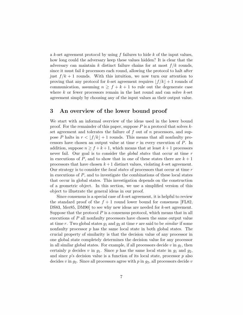
a k-set agreement protocol by using f failures to hide k of the input values,how long could the adversary keep these values hidden? It is clear that theadversary can maintain k distinct failure chains for at most f/k rounds,since it must fail k processors each round, allowing the protocol to halt afterjust f/k + 1 rounds. With this intuition, we now turn our attention toproving that any protocol for k-set agreement requires �f/k� + 1 rounds ofcommunication, assuming n ≥ f + k + 1 to rule out the degenerate casewhere k or fewer processors remain in the last round and can solve k-setagreement simply by choosing any of the input values as their output value.

3 An overview of the lower bound proof

We start with an informal overview of the ideas used in the lower boundproof. For the remainder of this paper, suppose P is a protocol that solves k-set agreement and tolerates the failure of f out of n processors, and sup-pose P halts in r < �f/k� + 1 rounds. This means that all nonfaulty pro-cessors have chosen an output value at time r in every execution of P . Inaddition, suppose n ≥ f + k + 1, which means that at least k + 1 processorsnever fail. Our goal is to consider the global states that occur at time rin executions of P , and to show that in one of these states there are k + 1processors that have chosen k + 1 distinct values, violating k-set agreement.Our strategy is to consider the local states of processors that occur at time rin executions of P , and to investigate the combinations of these local statesthat occur in global states. This investigation depends on the constructionof a geometric object. In this section, we use a simplified version of thisobject to illustrate the general ideas in our proof.

Since consensus is a special case of k-set agreement, it is helpful to reviewthe standard proof of the f + 1 round lower bound for consensus [FL82,DS83, Mer85, DM90] to see why new ideas are needed for k-set agreement.Suppose that the protocol P is a consensus protocol, which means that in allexecutions of P all nonfaulty processors have chosen the same output valueat time r. Two global states g1 and g2 at time r are said to be similar if somenonfaulty processor p has the same local state in both global states. Thecrucial property of similarity is that the decision value of any processor inone global state completely determines the decision value for any processorin all similar global states. For example, if all processors decide v in g1, thencertainly p decides v in g1. Since p has the same local state in g1 and g2,and since p’s decision value is a function of its local state, processor p alsodecides v in g2. Since all processors agree with p in g2, all processors decide v

7

in g2, and it follows that the decision value in g1 determines the decisionvalue in g2. A similarity chain is a sequence of global states, g1, . . . , g�,such that gi is similar to gi+1. A simple inductive argument shows that thedecision value in g1 determines the decision value in g�. The lower boundproof involves showing that two time r global states of P , one in which allprocessors start with 0 and one in which all processors start with 1, lie ona single similarity chain. Since there is a similarity chain from one state tothe other, processors must choose the same value in both states, violatingthe definition of consensus.

The problem with k-set agreement is that the decision values in oneglobal state do not determine the decision values in similar global states.If p has the same local state in g1 and g2, then p must choose the samevalue in both states, but the values chosen by the other processors are notdetermined. Even if n− 1 processors have the same local state in g1 and g2,the decision value of the last processor is still not determined. The fun-damental insight in this paper is that k-set agreement requires consideringall “degrees” of similarity at once, focusing on the number and identity oflocal states common to two global states. While this seems difficult—if notimpossible—to do using conventional graph theoretic techniques like sim-ilarity chains, there is a geometric generalization of similarity chains thatprovides a compact way of capturing all degrees of similarity simultaneously,and it is the basis of our proof.

A simplex is just the natural generalization of a triangle to n dimensions:for example, a 0-dimensional simplex is a vertex, a 1-dimensional simplex isan edge linking two vertices, a 2-dimensional simplex is a solid triangle, anda 3-dimensional simplex is a solid tetrahedron. We can represent a globalstate for an n-processor protocol as an (n− 1)-dimensional simplex [Cha93,HS99], where each vertex is labeled with a processor id and local state. If g1

and g2 are global states in which p1 has the same local state, then we “gluetogether” the vertices of g1 and g2 labeled with p1. Figure 4 shows howthese global states glue together in a simple protocol in which each of threeprocessors repeatedly sends its state to the others. Each process begins witha binary input. The first picture shows the possible global states after zerorounds: since no communication has occurred, each processor’s state consistsonly of its input. It is easy to check that the simplexes corresponding tothese global states form an octahedron. The next picture shows the complexafter one round. Each triangle corresponds to a failure-free execution, eachfree-standing edge to a single-failure execution, and so on. The third pictureshows the possible global states after three rounds.

The set of global states after an r-round protocol is quite complicated

8

Figure 4: Global states for zero, one, and two-round protocols.

9

Bermuda Triangle

Figure 5: The Bermuda Triangle is a highly-structured subcomplex of thesimplicial complex representing all global states of an r-round protocol, suchas the simplicial complexes illustrated in Figure 4 for the cases of zero, one,and two round protocols.

10

(P,a) (Q,b)

(R,c)

(S,d)

each simplex isconsistent with aglobal state

vertices labeled with (processor, local state)pairs

Figure 6: Bermuda Triangle with simplex representing typical global state.

11

ccccc

cccc?

ccccb

ccc?b

cc?bb

ccbbb

c?bbb

cbbbb

cccbb

?bbbb

bbbbb

cccc?

cccca

ccc?a

cccaa

cc?aa

ccaaa

c?aaa

caaaa

?aaaa

aaaaa

?aaaabaaaa

b?aaabbaaa

bb?aabbbaa

bbb?abbbba

bbbb?

cccaa

bbbaabb?aa

cc?aa

?bbaa

cbbaa

c?baa

ccbaa

cc?aa

?b?aa

cb?aa

c??aa

cc?aa

Figure 7: A simplified representation of the Bermuda Triangle for 5 proces-sors and a 1-round protocol for 2-set agreement. This representation omitsthe processor ids labeling the vertices to focus on how the local states changealong each dimension of the Bermuda Triangle.

(Figure 5), but it contains a well-behaved subset of global states which wecall the Bermuda Triangle B, since all fast protocols vanish somewhere inits interior. The Bermuda Triangle (Figure 6) is constructed by startingwith a large k-dimensional simplex, and triangulating it into a collection ofsmaller k-dimensional simplexes. We then label each vertex with an orderedpair (p, s) consisting of a processor identifier p and a local state s in sucha way that for each simplex T in the triangulation there is a global state gconsistent with the labeling of the simplex: for each ordered pair (p, s)labeling a corner of T , processor p has local state s in global state g.

To illustrate the process of labeling vertices, Figure 7 shows a simplifiedrepresentation of a two-dimensional Bermuda Triangle B. It is the BermudaTriangle for a protocol P for 5 processors solving 2-set agreement in 1 round.We have labeled grid points with local states, but we have omitted processorids and many intermediate nodes for clarity. The local states in the figureare represented by expressions such as bb?aa. Given 3 distinct input val-

12

Figure 8: Sperner’s Lemma.

ues a, b, c, we write bb?aa to denote the local state of a processor p at theend of a round in which the first two processors have input value b and sendmessages to p, the middle processor fails to send a message to p, and thelast two processors have input value a and send messages to p. In Figure 7,following any horizontal line from left to right across B, the input valuesare changed from a to b. The input value of each processor is changed—oneafter another—by first silencing the processor, and then reviving the pro-cessor with the input value b. Similarly, moving along any vertical line frombottom to top, processors’ input values change from b to c.

The complete labeling of the Bermuda Triangle B shown in Figure 7—which would include processor ids—has the following property. Let (p, s)be the label of a grid point x. If x is a corner of B, then s specifies thateach processor starts with the same input value, so p must choose this valueif it finishes protocol P in local state s. If x is on an edge of B, then sspecifies that each processor starts with one of the two input values labelingthe ends of the edge, so p must choose one of these values if it halts instate s. Similarly, if x is in the interior of B, then s specifies that eachprocessor starts with one of the three values labeling the corners of B, so pmust choose one of these three values if it halts in state s.

Now let us “color” each grid point with output values (Figure 8). Given

13

a grid point x labeled with (p, s), let us color x with the value v that pchooses in local state s at the end of P . This coloring of B has the propertythat the color of each of the corners is determined uniquely, the color ofeach point on an edge between two corners is forced to be the color ofone of the corners, and the color of each interior point can be the color ofany corner. Colorings with this property are called Sperner colorings, andhave been studied extensively in the field of algebraic topology. At thispoint, we exploit a remarkable combinatorial result first proved in 1928:Sperner’s Lemma [Spa66, p.151] states that any Sperner coloring of anytriangulated k-dimensional simplex must include at least one simplex whosecorners are colored with all k + 1 colors. In our case, however, this simplexcorresponds to a global state in which k + 1 processors choose k + 1 distinctvalues, which contradicts the definition of k-set agreement. Thus, in thecase illustrated above, there is no protocol for 2-set agreement halting in 1round.

We note that the basic structure of the Bermuda Triangle and the ideaof coloring the vertices with decision values and applying Sperner’s Lemmahave appeared in previous work by Chaudhuri [Cha91, Cha93]. In that work,she also proved a lower bound of �f/k�+ 1 rounds for k-set agreement, butfor a very restricted class of protocols. In particular, a protocol’s decisionfunction can depend only on vectors giving partial information about whichprocessors started with which input values, but cannot depend on any otherinformation in a processor’s local state, such as processor identities or mes-sage histories. The proof of her lower bound depends on this restrictionto a specific class of protocols. The technical challenge in this paper is toconstruct a labeling of vertices with processor ids and local states that willallow us to prove a lower bound for k-set agreement for arbitrary protocols.

Our approach consists of four parts. First, we construct long sequences ofglobal states that we call similarity chains, one chain for each pair of inputvalues. For example, for the pair of values a and b, we construct a longsequence of global states that begins with a global state in which all inputvalues are a, ends with a global state in which all input values are b, andin between systematically changes input values from a to b. These changesare made so gradually, however, that for any two adjacent global states inthe sequence, at most one processor can distinguish them; that is, they aresimilar to all other processors. Second, we label the points of B with globalstates. We label the points on each edge of B with a similarity chain ofglobal states. For example, consider the edge between the corner whereall processors start with input value a and the corner where all processorsstart with b. We label this edge with the similarity chain for a and b, as

14

described above. We label each remaining point using a combination of theglobal states on the edges. Third, we assign nonfaulty processors to pointsin such a way that the processor labeling a point has the same local statein the global states labeling all adjacent points. Finally, we project eachglobal state onto the associated nonfaulty processor’s local state, and labelthe point with the resulting processor-state pair.

4 The model

We use a synchronous, message-passing model with crash failures. Thesystem consists of n processors, p1, . . . , pn. Processors share a global clockthat starts at 0 and advances in increments of 1. Computation proceedsin a sequence of rounds, with round r lasting from time r − 1 to time r.Computation in a round consists of three phases: first each processor psends messages to some of the processors in the system, possibly includingitself, then it receives the messages sent to it during the round, and finallyit performs some local computation and changes state. We assume that thecommunication network is totally connected: every processor is able to senddistinct messages to every other processor in every round. We also assumethat communication is reliable (although processors can fail): if p sends amessage to q in round r, then the message is delivered to q in round r.

Processors follow a deterministic protocol that determines what messagesa processor should send and what output a processor should generate. Aprotocol has two components: a message component that maps a proces-sor’s local state to the list of messages it should send in the next round,and an output component that maps a processor’s local state to the outputvalue (if any) that it should choose. Processors can be faulty, however, andany processor p can simply stop in any round r. In this case, processor pfollows its protocol and sends all messages the protocol requires in rounds 1through r − 1, sends some subset of the messages it is required to send inround r, and sends no messages in rounds after r. We say that p is silentfrom round r if p sends no messages in round r or later. We say that p isactive through round r if p sends all messages required by the protocol inround r and earlier.

A full-information protocol is one in which every processor broadcasts itsentire local state to every processor, including itself, in every round [PSL80,FL82, Had83]. One nice property of full-information protocols is that everyexecution of a full-information protocol P has a compact representationcalled a communication graph [MT88]. The communication graph G for

15

0 1 2 3

redgreen

1p ,a

2p ,a

3p ,a

Figure 9: A three-round communication graph.

an r-round execution of P is a two-dimensional two-colored graph. Thevertices form an n × r grid, with processor names 1 through n labeling thevertical axis and times 0 through r labeling the horizontal axis. The noderepresenting processor p at time i is labeled with the pair 〈p, i〉. Given anypair of processors p and q and any round i, there is an edge between 〈p, i − 1〉and 〈q, i〉 whose color determines whether p successfully sends a message to qin round i: the edge is green if p succeeds, and red otherwise. In addition,each node 〈p, 0〉 is labeled with p’s input value. Figure 9 illustrates a threeround communication graph. In this figure, green edges are denoted by solidlines and red edges by dashed lines. We refer to the edge between 〈p, i − 1〉and 〈q, i〉 as the round i edge from p to q, and we refer to the node 〈p, i − 1〉as the round i node for p since it represents the point at which p sends itsround i messages. We define what it means for a processor to be silent oractive in terms of communication graphs in the obvious way.

In the crash failure model, a processor is silent in all rounds followingthe round in which it stops. This means that all communication graphsrepresenting executions in this model have the property that if a round iedge from p is red, then all round j ≥ i + 1 edges from p are red, whichmeans that p is silent from round i + 1. We assume that all communicationgraphs in this paper have this property, and we note that every r-roundgraph with this property corresponds to an r-round execution of P .

Since a communication graph G describes an execution of P , it also de-termines the global state at the end of P , so we sometimes refer to G as aglobal communication graph. In addition, for each processor p and time t,there is a subgraph of G that corresponds to the local state of p at the endround t, and we refer to this subgraph as a local communication graph. Thelocal communication graph for p at time t is the subgraph G(p, t) of G con-

16

taining all the information visible to p at the end of round t. Namely, G(p, t)is the subgraph induced by the node 〈p, t〉 and all prior nodes 〈q, t′〉 suchthat t′ < t and there is a path from 〈q, t′〉 to 〈p, t〉 consisting of 0 or 1 rededges followed by 0 or more green edges.

In the remainder of this paper, we use graphs to represent states. Wher-ever we used “state” in the informal overview of Section 3, we now substi-tute the word “graph.” Furthermore, we defined a full-information protocolto be a protocol in which processors broadcast their local states in everyround, but we now assume that processors broadcast the local communica-tion graphs representing these local states instead (as in [MT88]). In ad-dition, we assume that all executions of a full-information protocol run forexactly r rounds and produce output at exactly time r. All local and globalcommunication graphs are graphs at time r, unless otherwise specified.

The crucial property of a full-information protocol is that every protocolcan be simulated by a full-information protocol, and hence that we canrestrict attention to full-information protocols when proving the lower boundin this paper:

Lemma 4: If there is an n-processor protocol solving k-set agreement with ffailures in r rounds, then there is an n-processor full-information protocolsolving k-set agreement with f failures in r rounds.

5 Constructing the Bermuda Triangle

In this section, we define the basic geometric constructs used in our lowerbound proof. We begin with some preliminary definitions. A simplex S isthe convex hull of k +1 affinely-independent1 points x0, . . . , xk in Euclideanspace. This simplex is a k-dimensional volume, the k-dimensional analogueof a solid triangle or tetrahedron. The points x0, . . . , xk are called the ver-tices of S, and k is the dimension of S. We sometimes call S a k-simplexwhen we wish to emphasize its dimension. A simplex F is a face of S if thevertices of F form a subset of the vertices of S (which means that the di-mension of F is at most the dimension of S). A set of k-simplexes S1, . . . , S�

is a triangulation of S if S = S1 ∪ · · · ∪ S� and the intersection of Si and Sj

is a face of each2 for all pairs i and j. The vertices of a triangulation are1Points x0, . . . , xk are affinely independent if x1 −x0, . . . , xk − x0 are linearly indepen-

dent.2Notice that the intersection of two arbitrary k-dimensional simplexes Si and Sj will

be a volume of some dimension, but it need not be a face of either simplex.

17

Figure 10: Construction of Bermuda Triangle.

the vertices of the Si. Any triangulation of S induces triangulations of itsfaces in the obvious way.

The construction of the Bermuda Triangle is illustrated in Figure 10.Let B be the k-simplex in k-dimensional Euclidean space with vertices

(0, . . . , 0), (N, 0, . . . , 0), (N,N, 0, . . . , 0), . . . , (N, . . . ,N),

where N is a huge integer defined later in Section 6.3. The Bermuda Tri-angle B is a triangulation of B defined as follows. The vertices of B are thegrid points contained in B: these are the points of the form x = (x1, . . . , xk),where the xi are integers between 0 and N satisfying x1 ≥ x2 ≥ · · · ≥ xk.

Informally, the simplexes of the triangulation are defined as follows: pickany grid point and walk one step in the positive direction along each dimen-sion. The k + 1 points visited by this walk define the vertices of a simplex,one of the six simplexes illustrated in Figure 11 that can be glued togetherto form a unit cube. The triangulation B consists of all such simplexes

18

Figure 11: Simplex generation in Kuhn’s triangulation.

filling the interior of B. For example, the 2-dimensional Bermuda Triangleis illustrated in Figure 7. This triangulation, known as Kuhn’s triangu-lation, is defined formally as follows [Cha93]. Let e1, . . . , ek be the unitvectors; that is, ei is the vector (0, . . . , 1, . . . , 0) with a single 1 in the ithcoordinate. A simplex is determined by a point y0 and an arbitrary permu-tation f1, . . . , fk of the unit vectors e1, . . . , ek: the vertices of the simplexare the points yi = yi−1 + fi for all i > 0. When we list the vertices ofa simplex, we always write them in the order y0, . . . , yk in which they arevisited by the walk.

For brevity, we refer to the vertices of B as the corners of B. The“edges” of B are partitioned to form the edges of B. More formally, thetriangulation B induces triangulations of the one-dimensional faces (linesegments connecting the vertices) of B, and these induced triangulations arecalled the edges of B. The simplexes of B are called primitive simplexes.

Each vertex of B is labeled with an ordered pair (p,L) consisting of aprocessor id p and a local communication graph L. As illustrated in theoverview in Section 3, the crucial property of this labeling is that if S is aprimitive simplex with vertices y0, . . . , yk, and if each vertex yi is labeledwith a pair (qi,Li), then there is a global communication graph G such thateach qi is nonfaulty in G and has local communication graph Li in G.

Constructing this processor-graph labeling is the primary technical chal-lenge confronted in this paper, and the subject of the next three sections. Wegive a three-step procedure for labeling each vertex with a processor p and a

19

global communication graph G, and then we simply replace G with p’s localcommunication graph L in G to obtain the final labeling. In Section 6, weshow how to construct long chains of global communication graphs in whichadjacent graphs are nearly indistinguishable, and we use these sequences ofgraphs to label the vertices along the edges of the Bermuda Triangle. In Sec-tion 7, we show how to merge these graphs labeling vertices along the edgesto obtain the graphs labeling the interior vertices. Finally, in Section 8, weshow how to assign processors to vertices.

6 Step 1: Similarity chain construction

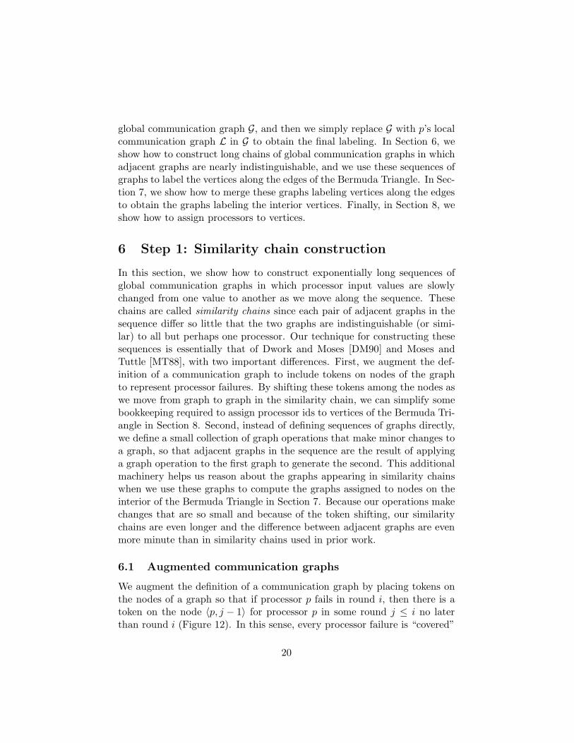
In this section, we show how to construct exponentially long sequences ofglobal communication graphs in which processor input values are slowlychanged from one value to another as we move along the sequence. Thesechains are called similarity chains since each pair of adjacent graphs in thesequence differ so little that the two graphs are indistinguishable (or simi-lar) to all but perhaps one processor. Our technique for constructing thesesequences is essentially that of Dwork and Moses [DM90] and Moses andTuttle [MT88], with two important differences. First, we augment the def-inition of a communication graph to include tokens on nodes of the graphto represent processor failures. By shifting these tokens among the nodes aswe move from graph to graph in the similarity chain, we can simplify somebookkeeping required to assign processor ids to vertices of the Bermuda Tri-angle in Section 8. Second, instead of defining sequences of graphs directly,we define a small collection of graph operations that make minor changes toa graph, so that adjacent graphs in the sequence are the result of applyinga graph operation to the first graph to generate the second. This additionalmachinery helps us reason about the graphs appearing in similarity chainswhen we use these graphs to compute the graphs assigned to nodes on theinterior of the Bermuda Triangle in Section 7. Because our operations makechanges that are so small and because of the token shifting, our similaritychains are even longer and the difference between adjacent graphs are evenmore minute than in similarity chains used in prior work.

6.1 Augmented communication graphs

We augment the definition of a communication graph by placing tokens onthe nodes of a graph so that if processor p fails in round i, then there is atoken on the node 〈p, j − 1〉 for processor p in some round j ≤ i no laterthan round i (Figure 12). In this sense, every processor failure is “covered”

20

0 1 2 3

redgreentoken

1p ,a

2p ,a

3p ,a

Figure 12: Three-round communication graph with one token per round.

by a token, and the number of processors failing in the graph is boundedfrom above by the number of tokens. In the next few sections, when weconstruct long sequences of these graphs, tokens will be moved betweenadjacent processors within a round, and used to guarantee that processorfailures in adjacent graphs change in a orderly fashion. For every value of �,we define graphs with exactly � tokens placed on nodes in each round, butwe will be most interested in the two cases with � equal to 1 and k.

For each value � > 0, we define an �-graph G, an augmented communi-cation graph, to be a communication graph with zero or more tokens placedon each node of the graph in a way that satisfies the following conditionsfor each round i, 1 ≤ i ≤ r:

1. The total number of tokens on round i nodes is exactly �.

2. If a round i edge from p is red, then there is a token on a round j ≤ inode for p.

3. If a round i edge from p is red, then p is silent from round i + 1.

We say that p is covered by a round i token if there is a token on the round inode for p, we say that p is covered in round i if p is covered by a round j ≤ itoken, and we say that p is covered in a graph if p is covered in any round.Similarly, we say that a round i edge from p is covered if p is covered inround i. The second condition says that every red edge is covered by atoken, and this together with the first condition implies that at most �rprocessors fail in an �-graph. In particular, when r ≤ f/k, at most kr ≤ fprocessors fail in a k-graph. We often refer to an �-graph as a graph whenthe value of � is clear from context or unimportant. We emphasize that the

21

tokens are simply an accounting trick, and have no meaning as part of theglobal or local state in the underlying communication graph.

We define a failure-free �-graph to be an �-graph in which all edges aregreen, and all round i tokens are on processor p1 in all rounds i.

6.2 Graph operations

We now define four operations on augmented graphs that make only minorchanges to a graph. In particular, the only change an operation makes is tochange the color of a single edge, to change the value of a single processor’sinput, or to move a single token between adjacent processors within thesame round. The operations are defined as follows (see Figure 13):

1. delete(i, p, q): This operation changes the color of the round i edgefrom p to q to red, and has no effect if the edge is already red. Thismakes the delivery of the round i message from p to q unsuccessful. Itcan only be applied to a graph if p and q are silent from round i + 1,and p is covered in round i.

2. add(i, p, q): This operation changes the color of the round i edgefrom p to q to green, and has no effect if the edge is already green.This makes the delivery of the round i message from p to q successful.It can only be applied to a graph if p and q are silent from round i+1,processor p is active through round i− 1, and p is covered in round i.

3. change(p, v): This operation changes the input value for processor pto v, and has no effect if the value is already v. It can only be appliedto a graph if p is silent from round 1, and p is covered in round 1.

4. move(i, p, q): This operation moves a round i token from 〈p, i − 1〉to 〈q, i − 1〉, and is defined only for adjacent processors p and q (thatis, {p, q} = {pj, pj+1} for some j). It can only be applied to a graphif p is covered by a round i token, and all red edges are covered byother tokens.

It is obvious from the definition of these operations that they preserve theproperty of being an �-graph: if G is an �-graph and τ is a graph operation,then τ(G) is an �-graph. We define delete, add, and change operations oncommunication graphs in exactly the same way, except that the conditionsof the form “p is covered in round i” are omitted.

22

0 1 2 3

2p ,a

3p ,a

1p ,a

delete(3, p , p )2 3

0 1 2 3

2p ,a

3p ,a

1p ,a

0 1 2 3

2p ,a

3p ,a

1p ,a

0 1 2 3

2p ,a

3p ,a

1p ,a

add(3, p , p )2 1

0 1 2 3

2p ,a

3p ,a

1p ,a

0 1 2 3

2p ,a

3p ,b

1p ,a

change(p , b)3

0 1 2 3

2p ,a

3p ,a

1p ,a

0 1 2 3

2p ,a

3p ,a

1p ,a

move(2, p , p )23

Figure 13: Operations on augmented communication graphs.

23

6.3 Graph sequences

We now define a sequence σ[v] of graph operations that can be applied toany failure-free graph G to transform it into the failure-free graph G[v] inwhich all processors have input v. It is crucial to our construction that thesesequences σ[v] differ only in the value v to which the input values are beingchanged by the sequence. For example, we might have two sequences

σ[a] = · · · delete(1, p, pn)change(p, a)add(1, p, pn) · · ·σ[b] = · · · delete(1, p, pn)change(p, b)add(1, p, pn) · · ·

changing input values to a and b, respectively, but these sequences are iden-tical except for the fact that the value a appears in one exactly where thevalue b appears in the other. For this reason, it is convenient to be ableto replace the values a and b appearing in the two sequences with a singlesymbol v and define a parameterized sequence

σ[v] = · · · delete(1, p, pn)change(p,v)add(1, p, pn) · · ·

so that the two sequences σ[a] and σ[b] can be obtained simply by replac-ing the symbol v with a and b, respectively. We define a parameterizedsequence σ[v] to be a sequence of graph operations with the symbol v ap-pearing as a parameter to some of the graph operations in the sequence. Inwhat follows, we will construct a parameterized sequence σ[v] with the prop-erty that for all values v and all graphs G, the sequence σ[v] transforms Ginto G[v].

Given a graph G, let red(G, p,m) and green(G, p,m) be graphs identicalto G except that all edges from p in rounds m, . . . , r are red and green,respectively. We define these graphs only if

1. p is covered in round m in G,

2. all faulty processors are silent from round m (or earlier) in G, and

3. all tokens are on p1 in rounds m + 1, . . . , r in G.

In addition, we define the graph green(G, p,m) only if

4. p is active through round m − 1 in G.

If G is an �-graph and red(G, p,m) and green(G, p,m) are both defined,then these conditions ensure that red(G, p,m) and green(G, p,m) are both �-graphs.

24

In the case of ordinary communication graphs, a result by Moses andTuttle [MT88] implies that there is a sequence of graphs called a “similaritychain” from G to red(G, p,m) and from G to green(G, p,m). In their proof—arefinement of similar proofs by Dwork and Moses [DM90] and others—thesequence of graphs they construct has the property that each graph in thechain can be obtained from the preceding graph by applying a sequenceof the add, delete, and change graph operations defined above. Essentiallythe same proof works for augmented communication graphs, provided weexpand the sequence of graph operations by inserting move operations be-tween the add, delete, and change operations to move the tokens among thenodes appropriately. With this modification, we can prove the following.Let faulty(G) be the set of processors that fail in G.

Lemma 5: For every processor p, round m, and set π of processors, thereare sequences silenceπ(p,m) and reviveπ(p,m) such that for all graphs G:

1. If red(G, p,m) is defined and π = faulty(G), then silenceπ(p,m)(G) =red(G, p,m).

2. If green(G, p,m) is defined and π = faulty(G), then reviveπ(p,m)(G) =green(G, p,m).

Proof: We proceed by reverse induction on m. Suppose m = r. Define

silenceπ(p, r) = delete(r, p, p1) · · · delete(r, p, pn)reviveπ(p, r) = add(r, p, p1) · · · add(r, p, pn).

For part 1, let G be any graph and suppose red(G, p, r) is defined. For each iwith 0 ≤ i ≤ n, let Gi be the graph identical to G except that the round redges from p to p1, . . . , pi are red. Since red(G, p, r) is defined, condition 1implies that p is covered in round r in G. Since p is covered in round r,each Gi−1 is a graph since it differs from G only in some new red edges from pin round r, and delete(r, p, pi) can be applied to Gi−1 to transform it to Gi.Since G = G0 and Gn = red(G, p, r), it follows that silenceπ(p, r) transforms Gto red(G, p, r). For part 2, let G be any graph and suppose green(G, p, r) isdefined. The proof of this part is the direct analogue of the proof of part 1.The only difference is that since we are coloring round r edges from p greeninstead of red, we must verify that p is active through round r− 1 in G, butthis follows immediately from condition 4.

Suppose m < r and the induction hypothesis holds for m+1. Define π′ =π ∪ {p} and define

set(m + 1, pi) = move(m + 1, p1, p2) · · ·move(m + 1, pi−1, pi)

25

reset(m + 1, pi) = move(m + 1, pi, pi−1) · · ·move(m + 1, p2, p1).

The set function moves the token from p1 to pi and the reset function movesthe token back from pi to p1.Define block(m, p, pi) to be delete(m, p, pi) if pi ∈ π′, and otherwise

set(m + 1, pi)silenceπ′(pi,m + 1) delete(m, p, pi) reviveπ′∪{pi}(pi,m + 1)

reset(m + 1, pi).

Define unblock(m, p, pi) to be add(m, p, pi) if pi ∈ π′, and otherwise

set(m + 1, pi)silenceπ′(pi,m + 1) add(m, p, pi) reviveπ′∪{pi}(pi,m + 1)

reset(m + 1, pi).

Finally, define

block(m, p) = block(m, p, p1) · · · block(m, p, pn)unblock(m, p) = unblock(m, p, p1) · · · unblock(m, p, pn)

and define

silenceπ(p,m) = silenceπ(p,m + 1) block(m, p)reviveπ(p,m) = silenceπ(p,m + 1)unblock(m, p) reviveπ′(p,m + 1).

For part 1, let G be any graph, and suppose red(G, p,m) is definedand π = faulty(G). Since red(G, p,m) is defined, the graph red(G, p,m+1) isalso defined, and the induction hypothesis for m+1 states that silenceπ(p,m+1) transforms G to red(G, p,m + 1). We will now show that block(m, p)transforms red(G, p,m + 1) to red(G, p,m), and we will be done. For each iwith 0 ≤ i ≤ n, let Gi be the graph identical to G except that p is silentfrom round m + 1 and the round m edges from p to p1, . . . , pi are red in Gi.Since red(G, p,m) is defined, condition 1 implies that p is covered in round min G. For each i with 0 ≤ i ≤ n, it follows that Gi really is a graph andthat π′ = faulty(Gi). Since red(G, p,m + 1) = G0 and Gn = red(G, p,m),it is enough to show that block(m, p, pi) transforms Gi−1 to Gi for each iwith 1 ≤ i ≤ n. The proof of this fact depends on whether pi ∈ π′, so weconsider two cases.

Consider the easy case with pi ∈ π′. We know that p is covered inround m in Gi−1 since it is covered in G by condition 1. We know that p issilent from round m + 1 in Gi−1 since it is silent in G0 = red(G, p,m + 1).

26

We know that pi is silent from round m + 1 in Gi−1 since pi ∈ π′ implies(assuming that pi is not just p again) that pi fails in G, and hence is silentfrom round m + 1 in G by condition 2. This means that block(m, p, pi) =delete(m, p, pi) can be applied to Gi−1 to transform Gi−1 to Gi.

Now consider the difficult case when pi ∈ π′. Let Hi−1 and Hi be graphsidentical to Gi−1 and Gi, except that a single round m + 1 token is on pi

in Hi−1 and Hi. Condition 3 guarantees that all round m + 1 tokens areon p1 in G, and hence in Gi−1 and Gi, so Hi−1 and Hi really are graphs.In addition, set(m + 1, pi) transforms Gi−1 to Hi−1, and reset(m + 1, pi)transforms Hi to Gi. Let Ii−1 and Ii be identical to Hi−1 and Hi exceptthat pi is silent from round m + 1 in Ii−1 and Ii. Processor pi is covered inround m+1 in Hi−1 and Hi, so Ii−1 and Ii really are graphs. In fact, pi doesnot fail in G since pi ∈ π′, so pi is active through round m in Ii−1 and Ii,so Ii−1 = red(Hi−1, pi,m + 1) and Hi = green(Ii, pi,m + 1). The inductivehypothesis for m+1 states that silenceπ′(pi,m+1) transforms Hi−1 to Ii−1,and reviveπ′∪{pi}(pi,m+1) transforms Ii to Hi. Finally, notice that the onlydifference between Ii−1 and Ii is the color of the round m edge from p to pi.Since p is covered in round m and p and pi are silent from round m + 1 inboth graphs, we know that delete(m, p, pi) transforms Ii−1 to Ii. It followsthat block(m, p, pi) transforms Gi−1 to Gi, and we are done.

For part 2, let G be any graph and suppose green(G, p,m) is definedand π = faulty(G). Since green(G, p,m) is defined, let G′ = green(G, p,m).Now let H and H′ be graphs identical to G and G′ except that p is silentfrom round m+1 in H and H′. Since green(G, p,m) is defined, processor p iscovered in round m in G by condition 1 and hence in G′, so H and H′ reallyare graphs. In addition, since green(G, p,m) is defined, processor p is activethrough round m − 1 in G by condition 4, so processor p is active throughround m in G′ and H′. This means that green(H′, p,m + 1) is defined, andin fact we have H = red(G, p,m + 1) and G′ = green(H′, p,m + 1). Theinduction hypothesis for m + 1 states that silenceπ(p,m + 1) transforms Gto H and that reviveπ′(p,m + 1) transforms H′ to G′. To complete theproof, we need only show that unblock(m, p) transforms H to H′. The proofof this fact is the direct analogue of the proof in part 1 that block(m, p)transforms red(G, p,m + 1) to red(G, p,m). The only difference is that sincewe are coloring round m edges from p with green instead of red, we mustverify that p is active through round m−1 in the graphs Hi analogous to Gi

in the proof of part 1, but this follows immediately from condition 4.Given a graph G, let Gi[v] be a graph identical to G, except that proces-

sor pi has input v. Using the preceding result, we can transform G to Gi[v].

27

Lemma 6: For each i, there is a parameterized sequence σi[v] with theproperty that for all values v and failure-free graphs G, the sequence σi[v]transforms G to Gi[v].

Proof: Define

set(1, pi) = move(1, p1, p2) · · ·move(1, pi−1, pi)reset(1, pi) = move(1, pi, pi−1) · · ·move(1, p2, p1)

and define

σi[v] = set(1, pi)silence∅(pi, 1)change(pi,v)revive{pi}(pi, 1)reset(1, pi)

where ∅ denotes the empty set. Now consider any value v and any failure-free graph G, and let G′ = Gi[v]. Since G and G′ are failure-free graphs, allround 1 tokens are on p1, so let H and H′ be graphs identical to G and G′

except that a single round 1 token is on pi in H and H′. We know that Hand H′ are graphs, and that set(1, pi) transforms G to H and reset(1, pi)transforms H′ to G′. Since pi is covered in H and H′, let I and I ′ beidentical to H and H′ except that pi is silent from round 1. We knowthat I and I ′ are graphs, and it follows by Lemma 5 that silence∅(pi, 1)transforms H to I and that revive{pi}(pi, 1) transforms I ′ to H′. Finally,notice that I and I ′ differ only in the input value for pi. Since pi is coveredand silent from round 1 in both graphs, the operation change(pi, v) can beapplied to I and transforms it to I ′. Concatenating these transformations,it follows that σi[v] transforms G to G′ = Gi[v].

By concatenating such operation sequences, we can transform G into G[v]by changing processors’ input values one at a time:

Lemma 7: Let σ[v] = σ1[v] · · · σn[v]. For every value v and failure-freegraph G, the sequence σ[v] transforms G to G[v].

Now we can define the parameter N used in defining the shape of B: N isthe length of the sequence σ[v], which is exponential in r.

7 Step 2: Graph assignment

In this section, we label each vertex of B with an augmented global com-munication graph. Speaking informally, we use each sequence σ[vi] of graphoperations to generate a sequence of graphs, and then use this sequence ofgraphs to label the vertices along the edge of the Bermuda Triangle in the ithdimension. To label the vertices on the interior of the Bermuda Triangle,we define an operation to “merge” graphs labeling the edges into a singlegraph.

28

7.1 Graph merge

We begin with the definition of the operation merging a sequence of graphsinto a single graph.

The merge of a sequence H1, . . . ,Hk of graphs is a graph defined asfollows:

1. an edge e is colored red if it is red in any of the graphs H1, . . . ,Hk,and green otherwise, and

2. an initial node 〈p, 0〉 is labeled with the value vi where i is the maxi-mum index such that 〈p, 0〉 is labeled with vi in Hi, or v0 if no such iexists, and

3. the number of tokens on a node 〈p, i〉 is the sum of the number oftokens on the node in the graphs H1, . . . ,Hk.

The first condition says that a message is missing in the resulting graph ifand only if it is missing in any of the merged graphs. To understand thesecond condition, let x = (x1, . . . , xk) be a vertex of B and let Hi be theresult of applying the first xi operations in σ[vi] to some fixed graph G. Itfollows from the construction of σ[v] that there is a single integer c with theproperty that it is the cth graph operation in σ[vi] that changes p’s inputto vi for each i. Since x = (x1, . . . , xk) is a vertex of B, the indices xi

are ordered by x1 ≥ x2 ≥ · · · ≥ xk. It follows that p’s input has beenchanged to vi in Hi for those i = 1, . . . , j satisfying xi ≥ c and not in Hi forthose i = j + 1, . . . , k satisfying c > xi. The second condition above is justa compact way of identifying this final value vj.

One important property of the merge operator is that merging a sequenceof 1-graphs yields a k-graph, where k is the length of the sequence of 1-graphs:

Lemma 8: Let H be the merge of the graphs H1, . . . ,Hk. If H1, . . . ,Hk

are 1-graphs, then H is a k-graph.

Proof: We consider the three conditions required of a k-graph in turn.First, there are k tokens in each round of H since there is 1 token in eachround of each graph H1, . . . ,Hk. Second, every red edge in H is covered bya token since every red edge in H corresponds to a red edge in one of thegraphs Hj, and this edge is covered by a token in Hj. Third, if there is ared edge from p in round i in H, then there is a red edge from p in round i

29

of one of the graphs Hj. In this graph, p is silent from round i + 1, so thesame is true in H. Thus, H is a k-graph.

Remember that at most kr ≤ f processors fail in a k-graph like H.

7.2 Graph assignment

Now we can define the assignment of graphs to vertices of B. For eachinput value vi, let Fi be the failure-free 1-graph in which all processorshave input vi. Let x = (x1, . . . , xk) be an arbitrary vertex of B. For eachcoordinate xj, let σj be the prefix of σ[vj ] consisting of the first xj operations,and let Hj be the 1-graph resulting from the application of σj to Fj−1. Thismeans that in Hj , some set p1, . . . , pi of adjacent processors have had theirinputs changed from vj−1 to vj. The graph G labeling x is defined to be themerge of H1, . . . ,Hk. We know that G is a k-graph by Lemma 8, and hencethat at most rk ≤ f processors fail in G.

Remember that we always write the vertices of a primitive simplex ina canonical order y0, . . . , yk. In the same way, we always write the graphslabeling the vertices of a primitive simplex in the canonical order G0, . . . ,Gk,where Gi is the graph labeling yi.

7.3 Graph consistency

The graphs labeling the vertices of a primitive simplex have some convenientproperties. For this section, fix a primitive simplex S, let y0, . . . , yk be thevertices of S, and let G0, . . . ,Gk be the graphs labeling the correspondingvertices of S. Our first result says that any processor that is uncovered at avertex of S is nonfaulty at all vertices of S.

Lemma 9: If processor q is not covered in the graph labeling a vertex of S,then q is nonfaulty in the graph labeling every vertex of S.

Proof: Suppose to the contrary that q is faulty in some graph labeling avertex of S. Let y0 = (a1, . . . , ak) be the first vertex of S. For each i,let σi and σiτi be the prefixes of σ[vi] consisting of the first ai and ai + 1operations, and let Hi and H′

i be the result of applying σi and σiτi to Fi−1.For each i, we know that the graph Gi labeling the vertex yi of S is the mergeof graphs I i

1, . . . ,I ik where I i

j is either Hj or H′j. Suppose q is faulty in Gi.

Then q must be faulty in some graph I ij in the sequence of graphs I i

1, . . . ,I in

merged to form Gi, so q must fail in one of the graphs Hj or H′j. Since σj

and σjτj are prefixes of σ[vj ], it is easy to see from the definition of σ[vj ] that

30

the fact that q fails in one of the graphs Hj and H′j implies that q is covered

in both graphs. Since one of these graphs is contained in the sequence ofgraphs merged to form Ga for each a, it follows that q is covered in each Ga.This contradicts the fact that q is uncovered in a graph labeling a vertexof S.

Our next result shows that we can use the bound on the number oftokens to bound the number of processors failing at any vertex of S.

Lemma 10: If Fi is the set of processors failing in Gi and F = ∪iFi,then |F | ≤ rk ≤ f .

Proof: If q ∈ F , then q ∈ Fi for some i and q fails in Gi, so q is coveredin every graph labeling every vertex of S by Lemma 9. It follows that eachprocessor in F is covered in each graph labeling S. Since there are at most rktokens to cover processors in any graph, there are at most rk processors in F .

We have assigned graphs to S, and now we must assign processorsto S. A local processor labeling of S is an assignment of distinct proces-sors q0, . . . , qk to the vertices y0, . . . , yk of S so that qi is uncovered in Gi

for each yi. A global processor labeling of B is an assignment of processorsto vertices of B that induces a local processor labeling at each primitivesimplex. The final important property of the graphs labeling S is that ifwe use a processor labeling to label S with processors, then S is consistentwith a single global communication graph. The proof of this requires a fewpreliminary results.

Lemma 11: If Gi−1 and Gi differ in p’s input value, then p is silent fromround 1 in G0, . . . ,Gk. If Gi−1 and Gi differ in the color of an edge from qto p in round t, then p and q are silent from round t + 1 in G0, . . . ,Gk.

Proof: Suppose the two graphs Gi−1 and Gi labeling vertices yi−1 and yi

differ in the input to p at time t = 0 or in the color of an edge from qto p in round t. The vertices differ in exactly one coordinate j, so yi−1 =(a1, . . . , aj , . . . , ak) and yi = (a1, . . . , aj +1, . . . , ak). For each �, let σ� be theprefix of σ[v�] consisting of the first a� operations, and let H0

� be the resultof applying σ� to F�−1. Furthermore, in the special case of � = j, let σjτj

be the prefix of σ[vj ] consisting of the first aj + 1 operations, and let H1j be

the result of applying σjτj to Fj−1.We know that Gi−1 is the merge of H0

1, . . . ,H0j , . . . ,H0

k, and that Gi isthe merge of H0

1, . . . ,H1j , . . . ,H0

k. If H0j and H1

j are equal, then Gi−1 and Gi

31

are equal. Thus, H0j and H1

j must differ in the input to p at time t = 0 orin the color of an edge between q and p in round t, exactly as Gi−1 and Gi

differ. Since H0j and H1

j are the result of applying σj and σjτj to Fj−1, thischange at time t must be caused by the operation τj . It is easy to see fromthe definition a graph operation like τj that (1) if τj changes p’s input value,then p is silent from round 1 in H0

j and H1j , and (2) if τj changes the color

of an edge from q to p in round t, then p and q are silent from round t + 1in H0

j and H1j . Consequently, the same is true in the merged graphs Gi−1

and Gi.

Lemma 12: If Gi−1 and Gi differ in the local communication graph of p attime t, then p is silent from round t + 1 in G0, . . . ,Gk.

Proof: We proceed by induction on t. If t = 0, then the two graphs mustdiffer in the input to p at time 0, and Lemma 11 implies that p is silent fromround 1 in the graphs G0, . . . ,Gk labeling the simplex. Suppose t > 0 andthe inductive hypothesis holds for t − 1. Processor p’s local communicationgraph at time t can differ in the two graphs for one of two reasons: either phears from some processor q in round t in one graph and not in the other,or p hears from some processor q in both graphs but q has different localcommunication graphs at time t − 1 in the two graphs. In the first case,Lemma 11 implies that p is silent from round t + 1 in the graphs G0, . . . ,Gk.In the second case, the induction hypothesis for t− 1 implies that q is silentfrom round t in the graphs G0, . . . ,Gk. In particular, q is silent in round tin Gi−1 and Gi, so it is not possible for p to hear from q in round t in bothgraphs, and this case is impossible.

Lemma 13: If p sends a message in round r in any of the graphs G0, . . . ,Gk,then p has the same local communication graph at time r − 1 in all of thegraphs G0, . . . ,Gk.

Proof: If p has different local communication graphs at time r − 1 in twoof the graphs G0, . . . ,Gk, then there are two adjacent graphs Gi−1 and Gi

in which p has different local communication graphs at time r − 1. ByLemma 12, p is silent in round r in all of the graphs G0, . . . ,Gk, contradictingthe hypothesis that p sent a round r message in one of them.

Finally, we can prove the crucial property of primitive simplexes in theBermuda Triangle:

32

Lemma 14: Given a local processor labeling, let q0, . . . , qk be the proces-sors labeling the vertices of S, and let Li be the local communication graphof qi in Gi. There is a global communication graph G with the property thateach qi is nonfaulty in G and has the local communication graph Li in G.

Proof: Let Q be the set of processors that send a round r message inany of the graphs G0, . . . ,Gk. Notice that this set includes the uncoveredprocessors q0, . . . , qk, since Lemma 9 says that these processors are nonfaultyin each of these graphs. For each processor q ∈ Q, Lemma 13 says that q hasthe same local communication graph at time r− 1 in each graph G0, . . . ,Gk.

Let H be the global communication graph underlying any one of thesegraphs. Notice that each processor q ∈ Q is active through round r − 1in H. To see this, notice that since q sends a message in round r in one ofthe graphs labeling S, it sends all messages in round r − 1 in that graph.On the other hand, if q fails to send a message in round r − 1 in H, thenthe same is true for the corresponding graph labeling S. Thus, there areadjacent graphs Gi−1 and Gi labeling S where p sends a round r−1 messagein one and not in the other. Consequently, Lemma 11 says q is silent inround r in all graphs labeling S, but this contradicts the fact that q doessend a round r message in one of these graphs.

Now let G be the global communication graph obtained from H by col-oring green each round r edge from each processor q ∈ Q, unless the edgeis red in one of the local communication graphs L0, . . . ,Lk in which casewe color it red in G as well. Notice that since the processors q ∈ Q areactive through round r − 1 in H, changing the color of a round r edge froma processor q ∈ Q to either red or green is acceptable, provided we do notcause more that f processors to fail in the process. Fortunately, Lemma 10implies that there are at least n − rk ≥ n − f processors that do not failin any of the graphs G0, . . . ,Gk. This means that there is a set of n − fprocessors that send to every processor in round r of every graph Gi, and inparticular that the round r edges from these processors are green in everylocal communication graph Li. It follows that for at least n − f proces-sors, all round r edges from these processors are green in G, so at most fprocessors fail in G.

Each processor qi is nonfaulty in G, since qi is nonfaulty in each G0, . . . ,Gk,meaning each edge from qi is green in each G0, . . . ,Gk and L0, . . . ,Lk, andtherefore in G. In addition, each processor qi has the local communicationgraph Li in G. To see this, notice that Li consists of a round r edge from pj

to qi for each j, and the local communication graph for pj at time r − 1 ifthis edge is green. This edge is green in Li if and only if it is green in G.

33

In addition, if this edge is green in Li, then it is green in Gi. In this case,Lemma 13 says that pj has the same local communication graph at time r−1in each graph G0, . . . ,Gk, and therefore in G. Consequently, qi has the localcommunication graph Li in G.

8 Step 3: Processor assignment

What Lemma 14 at the end of the preceding section tells us is that all wehave left to do is to construct a global processor labeling. In this section,we show how to do this. We first associate a set of “live” processors witheach communication graph labeling a vertex of B, and then we choose oneprocessor from each set to label each vertex of B.

8.1 Live processors

Given a graph G, we construct a set of c = n − rk ≥ k + 1 uncovered(and hence nonfaulty) processors. We refer to these processors as the liveprocessors in G, and we denote this set by live(G). These live sets have onecrucial property: if G and G′ are two graphs labeling adjacent vertices, andif p is in both live(G) and live(G′), then p has the same rank in both sets.As usual, we define the rank of pi in a set R of processors to be the numberof processors pj ∈ R with j ≤ i.

Given a graph G, we now show how to construct live(G). This construc-tion has one goal: if G and G′ are graphs labeling adjacent vertices, thenthe construction should minimize the number of processors whose rank dif-fers in the sets live(G) and live(G′). The construction of live(G) begins withthe set of all processors, and removes a set of rk processors, one for eachtoken. This set of removed processors includes the covered processors, butmay include other processors as well. For example, suppose pi and pi+1 arecovered with one token each in G, but suppose pi is uncovered and pi+1 iscovered by two tokens in G′. For simplicity, let’s assume these are the onlytokens on the graphs. When constructing the set live(G), we remove both pi

and pi+1 since they are both covered. When constructing the set live(G′),we remove pi+1, but we must also remove a second processor correspondingto the second token covering pi+1. Which processor should we remove? Ifwe choose a low processor like p1, then we have changed the rank of a lowprocessor like p2 from 2 to 1. If we choose a high processor like pn, then wehave changed the rank of a high processor like pn−1 from n− 3 to n− 2. Onthe other hand, if we choose to remove pi again, then no processors change

34

S ← {1, . . . , n}for each i = 1, . . . , n

count ← 0for each j = i, i − 1, . . . , 1, i + 1, . . . , n

if count = mi then breakif j ∈ S then

S ← S − {j}count ← count + 1

live(G) ← S

Figure 14: The construction of live(G).

rank. In general, the construction of live(G) considers each processor p inturn. If p is covered by mp tokens in G, then the construction removes mp

processors by starting with p, working down the list of remaining processorssmaller than p, and then working up the list of processors larger than p ifnecessary.

Specifically, given a graph G, the multiplicity of p is the number mp oftokens appearing on nodes for p in G, and the multiplicity of G is the vec-tor m = 〈mp1 , . . . ,mpn〉. Given the multiplicity of G as input, the algorithmgiven in Figure 14 computes live(G). In this algorithm, processor pi is de-noted by its index i. We refer to the ith iteration of the main loop as the ithstep of the construction. This construction has two obvious properties:

Lemma 15: If i ∈ live(G) then

1. i is uncovered : mi = 0

2. room exists under i:∑i−1

j=1 mj ≤ i − 1

Proof: Suppose i ∈ live(G). For part 1, if mi > 0 then i will be re-moved by step i if it has not already removed by an earlier step, contradict-ing i ∈ live(G). For part 2, notice that steps 1 through i − 1 remove a totalof

∑i−1j=1 mj values. If this sum is greater than i − 1, then it is not possible

for all of these values to be contained in 1, . . . , i − 1, so i will be removedwithin the first i − 1 steps, contradicting i ∈ live(G).

The assignment of graphs to the corners of a simplex has the propertythat once p becomes covered on one corner of S, it remains covered on thefollowing corners of S:

35

Lemma 16: If p is uncovered in the graphs Gi and Gj, where i < j, then pis uncovered in each graph Gi,Gi+1, . . . ,Gj .

Proof: If p is covered in G� for some � between i and j, then p is uncoveredin G�−1 and covered in G� for some � between i and j. Since G�−1 and G�

are on adjacent vertices of the simplex, the sequences of graphs merged toconstruct them are of the form H1, . . . ,Hm, . . . ,Hk and H1, . . . ,H′

m, . . . ,Hk,respectively, for some m. Since p is uncovered in G�−1 and covered in G�, itmust be that p is uncovered in Hm and covered in H′

m. Notice, however,that H′

m is used in the construction of each graph G�,G�+1, . . . ,Gj . Thismeans that p is covered in each of these graphs, contradicting the fact that pis uncovered in Gj.

Finally, because token placements in adjacent graphs on a simplex differin at most the movement of one token from one processor to an adjacentprocessor, we can use the preceding lemma to prove the following:

Lemma 17: If p ∈ live(Gi) and p ∈ live(Gj), then p has the same rankin live(Gi) and live(Gj).

Proof: Assume without loss of generality that i < j. Since p ∈ live(Gi)and p ∈ live(Gj), Lemma 15 implies that p is uncovered in the graphs Gi

and Gj , and Lemma 16 implies that p is uncovered in Gi,Gi+1, . . . ,Gj . Sincetoken placements in adjacent graphs differ in at most the movement of onetoken from one processor to an adjacent processor, and since p is uncoveredin all of these graphs, this means that the number of tokens on proces-sors smaller than p is the same in all of these graphs. Specifically, thesum

∑p−1�=1 m� of multiplicities of processors smaller than p is the same

in Gi,Gi+1, . . . ,Gj . In particular, Lemma 15 implies that this sum is thesame value s ≤ p − 1 in Gi and Gj , so p has the same rank p − s in live(Gi)and live(Gj).

8.2 Processor assignment

We now choose one processor from each set live(G) to label the vertex withgraph G. Given a vertex x = (x1, . . . , xk), we define

plane(x) =k∑

i=1

xi (mod k + 1)

.

36

Lemma 18: plane(x) = plane(y) if x and y are distinct vertices of the samesimplex.

Proof: Since x and y are in the same simplex, we can write y = x +f1 + · · · + fj for some distinct unit vectors f1, . . . , fj and some 1 ≤ j ≤ k.If x = (x1, . . . , xk) and y = (y1, . . . , yk), then the sums

∑ki=1 xi and

∑ki=1 yi

differ by exactly j. Since 1 ≤ j ≤ k and since planes are defined as sumsmodulo k + 1, we have plane(x) = plane(y).

We define a global processor labeling π as follows: given a vertex xlabeled with a graph G, we define π to map x to the processor havingrank plane(x) in live(G).

Lemma 19: The mapping π is a global processor labeling.

Proof: First, it is clear that π maps each vertex x labeled with a graph Gx

to a processor qx that is uncovered in Gx. Second, π maps distinct verticesof a simplex to distinct processors. To see this, suppose to the contrary thatboth x and y are labeled with p, and let Gx and Gy be the graphs labeling xand y. We know that the rank of p in live(Gx) is plane(x) and that therank of p in live(Gy) is plane(y), and we know that p has the same rankin live(Gx) and live(Gy) by Lemma 17. Consequently, plane(x) = plane(y),contradicting Lemma 18.

We label the vertices of B with processors according to the processorlabeling π.

Now that we have assigned a global communication graph G and a proces-sor p to each vertex x of the Bermuda Triangle, let us replace the pair (p,G)labeling x with the pair (p,L) where L is processor p’s local communica-tion graph in G. The following result is a direct consequence of Lemmas 14and 19. It says that the local communication graphs of processors labelingthe corners of a simplex are consistent with a single global communicationgraph.

Lemma 20: Let q0, . . . , qk and L0, . . . ,Lk be the processors and local com-munication graphs labeling the vertices of a simplex. There is a globalcommunication graph G with the property that each qi is nonfaulty in Gand has the local communication graph Li in G.

9 Finishing the proof with Sperner’s Lemma

We now state Sperner’s Lemma, and use it to prove a lower bound on thenumber of rounds required to solve k-set agreement.

37

Notice that the corners of B are points ci of the form (N, . . . ,N, 0, . . . , 0)with i indices of value N for 0 ≤ i ≤ k. For example, c0 = (0, . . . , 0), c1 =(N, 0, . . . , 0), and ck = (N, . . . ,N). Informally, a Sperner coloring of Bassigns a color to each vertex so that each corner vertex ci is given a distinctcolor wi, each vertex on the edge between ci and cj is given either wi or wj ,and so on.

More formally, let S be a simplex and let F be a face of S. Any trian-gulation of S induces a triangulation of F in the obvious way. Let T be atriangulation of S. A Sperner coloring of T assigns a color to each vertexof T so that each corner of T has a distinct color, and so that the verticescontained in a face F are colored with the colors on the corners of F , foreach face F of T . Sperner colorings have a remarkable property: at leastone simplex in the triangulation must be given all possible colors.

Lemma 21 (Sperner’s Lemma): If B is a triangulation of a k-simplex,then for any Sperner coloring of B, there exists at least one k-simplex in Bwhose vertices are all given distinct colors.

Let P be the protocol whose existence we assumed in the previous sec-tion. Define a coloring χP of B as follows. Given a vertex x labeled withprocessor p and local communication graph L, color x with the value vthat P requires processor p to choose when its local communication graphis L. This coloring is clearly well-defined, since P is a protocol in which allprocessors chose an output value at the end of round r. We will now expandthe argument sketched in the introduction to show that χP is a Spernercoloring.

We first prove a simple claim. Recall that B is the simplex whose verticesare the corner vertices c0, . . . , ck, and that B is a triangulation of B. Let Fbe some face of B not containing the corner ci, and let F denote the tri-angulation of F induced by B. We prove the following technical statementabout vertices in F .

Claim 22: If x = (x1, . . . , xk) is a vertex of a face F not containing ci, then

1. if i = 0, then x1 = N ,

2. if 0 < i < k, then xi+1 = xi, and

3. if i = k, then xk = 0.

Proof: Each vertex x of B can be expressed using barycentric coordinateswith respect to the corner vertices: that is, x = α0c0 + · · ·+αkck, where 0 ≤

38

αj ≤ 1 for 0 ≤ j ≤ k and∑k

i=0 αi = 1. Since x is a vertex of a face F notcontaining the corner ci, it follows that αi = 0. We consider the three cases.Case 1: i = 0. Each corner c1, . . . , ck has the value N in the first position.Since α0 = 0, the value in the first position of α0c0 + · · · + αkck is (α1 +· · · + αk)N = N .Case 2: 0 < i < k. Each corner c0, . . . , ci−1 has 0 in positions i and i+1, andeach corner ci+1, . . . , ck has N in positions i and i+1. Since αi = 0, the linearcombination α0c0 + · · · + αkck will have the same value (αi+1 + · · · + αk)Nin positions i and i + 1. Thus, xi = xi+1.Case 3: i = k. Each corner c0, . . . , ck−1 has 0 in position k. Since αk = 0,the value in the kth position of α0c0 + · · · + αkck is 0. Thus, xk = 0.

Lemma 23: If P is a protocol for k-set agreement tolerating f faults andhalting in r ≤ �f/k� rounds, then χP is a Sperner coloring of B.

Proof: We must show that χP satisfies the two conditions of a Spernercoloring.

For the first condition, consider any corner vertex ci. Remember that ci

was originally labeled with the 1-graph Fi describing a failure-free executionin which all processors start with input vi, and that the local communicationgraph L labeling ci is a subgraph of Fi. Since the validity condition of the k-set agreement problem requires that any value chosen by a processor mustbe an input value of some processor, all processors must chose vi in Fi, andit follows that the vertex ci must be colored with vi. This means that eachcorner ci is colored with a distinct value vi.

For the second condition, consider any face F of B, and let us prove thatvertices in F are colored with the colors on the corners of F . Equivalently,suppose that ci is not a corner of F , and let us prove that no vertex in F iscolored with vi.

Consider the global communication graph G originally labeling a vertex xof F , and the graphs H1, . . . ,Hk used in the merge defining G. The definitionof this merge says that the input value labeling a node 〈p, 0〉 in G is vm

where m is the maximum m such that 〈p, 0〉 is labeled with vm in Hm, or v0

if no such m exists. Again, we consider three cases. In each case, we showthat no processor in G has the input value vi.

Suppose i = 0. Since x1 = N by Claim 22, we know that H1 = F1,where the input value of every processor is v1. By the definition of themerge operation, it follows immediately that no processor in G can haveinput value v0.

39

Suppose 1 < i < k. Again, xi+1 = xi by Claim 22. Now, Hi is the resultof applying σi, the first xi operations of σ[vi], to the graph Fi−1. Simi-larly, Hi+1 is the result of applying σi+1, the first xi+1 operations of σ[vi+1],to the graph Fi. Since xi+1 = xi, both σi and σi+1 are of the same length,and it follows that σi contains an operation of the form change(p, vi) if andonly if σi+1 contains an operation of the form change(p, vi+1). This impliesthat for any processor, either its input value is vi−1 in Hi and vi in Hi+1,or its input value is vi in Hi and vi+1 in Hi+1. In both cases, vi is not theinput value of this processor.

Suppose i = k. Since xk = 0 by Claim 22, we know that Hk = Fk−1,where the input value of every processor is vk−1. By the definition of merge,it follows immediately that no processor in G can have input value vk.

Therefore, we have shown that if x is a vertex of a face F of B, and ci

is not a corner vertex of F , then the communication graph G correspondingto x contains no processor with input value vi. Therefore, by the validitycondition, the value chosen at this vertex cannot be vi, and it follows that xis assigned a color other than vi. So, x must be colored by a color vj suchthat cj is a corner vertex of F . Since cj is colored vj , the second conditionof Sperner’s Lemma holds. So χP is a Sperner coloring.

Sperner’s Lemma guarantees that some primitive simplex is colored by k+1 distinct values, and this simplex corresponds to a global state in which k+1processors choose k + 1 distinct values, contradicting the definition of k-setagreement:

Theorem 24: If n ≥ f + k + 1, then no protocol for k-set agreement canhalt in fewer than �f/k� + 1 rounds.

Proof: Suppose P is a protocol for k-set agreement tolerating f faults andhalting in r ≤ �f/k� rounds, and consider the corresponding Bermuda Tri-angle B. Lemma 23 says that χP is a Sperner coloring of B, so Sperner’sLemma 21 says that there is a simplex S whose vertices are colored with k+1distinct values v0, . . . , vk. Let q0, . . . , qk and L0, . . . ,Lk be the processors andlocal communication graphs labeling the corners of S. By Lemma 20, thereexists a communication graph G in which qi is nonfaulty and has local com-munication graph Li. This means that G is a time r global communicationgraph of P in which each qi must choose the value vi. In other words, k + 1processors must choose k + 1 distinct values, contradicting the fact that Psolves k-set agreement in r rounds.

40

Acknowledgments

We are grateful to two anonymous referees for a number of suggestions lead-ing to significant improvements in this paper. The results in the paper haveappeared earlier in preliminary form. The lower bound result has appearedin [CHLT93] and the algorithm has appeared in [Cha91]. Much of this workwas performed while the first author was visiting MIT. The first and thirdauthors were supported in part by NSF grant CCR-89-15206, in part byDARPA contracts N00014-89-J-1988, N00014-92-J-4033, and N00014-92-J-1799, and in part by ONR contract N00014-91-J-1046. In addition, the firstauthor was supported in part by NSF grant CCR-93-08103.

References

[AR96] Hagit Attiya and Sergio Rajsbaum. The combinatorial structureof wait-free solvable tasks. In Proceedings of the 10th Interna-tional Workshop on Distributed Algorithms, volume 1151 of Lec-ture Notes in Computer Science, pages 322–343. Springer-Verlag,Berlin, October 1996.

[BG93] Elizabeth Borowsky and Eli Gafni. Generalized FLP impossi-bility result for t-resilient asynchronous computations. In Pro-ceedings of the 25th ACM Symposium on Theory of Computing,pages 91–100, May 1993.

[BHG87] Philip A. Bernstein, Vassos Hadzilacos, and Nathan Good-man. Concurrency Control and Recovery in Database Systems.Addison-Wesley Publishing Company, Reading, Massachusetts,1987.

[Cha91] Soma Chaudhuri. Towards a complexity hierarchy of wait-freeconcurrent objects. In Proceedings of the 3rd IEEE Symposiumon Parallel and Distributed Processing, December 1991.

[Cha93] Soma Chaudhuri. More choices allow more faults: Set consen-sus problems in totally asynchronous systems. Information andComputation, 105(1):132–158, July 1993.

[CHLT93] Soma Chaudhuri, Maurice Herlihy, Nancy Lynch, and Mark R.Tuttle. A tight lower bound for k-set agreement. In Proceedings ofthe 34th IEEE Symposium on Foundations of Computer Science,pages 206–215, November 1993.

41

[DM90] Cynthia Dwork and Yoram Moses. Knowledge and commonknowledge in a Byzantine environment: Crash failures. Infor-mation and Computation, 88(2):156–186, October 1990.

[Dol82] Danny Dolev. The Byzantine generals strike again. Journal ofAlgorithms, 3(1):14–30, March 1982.

[DS83] Danny Dolev and H. Raymond Strong. Authenticated algo-rithms for Byzantine agreement. SIAM Journal on Computing,12(3):656–666, November 1983.

[Fis83] Michael J. Fischer. The consensus problem in unreliable dis-tributed systems (a brief survey). In Marek Karpinsky, editor,Proceedings of the 10th International Colloquium on Automata,Languages, and Programming, pages 127–140. Springer-Verlag,1983.

[FL82] Michael J. Fischer and Nancy A. Lynch. A lower bound for thetime to assure interactive consistency. Information ProcessingLetters, 14(4):183–186, June 1982.

[FLP85] Michael J. Fischer, Nancy A. Lynch, and Michael S. Paterson.Impossibility of distributed consensus with one faulty processor.Journal of the ACM, 32(2):374–382, 1985.

[GK99] Eli Gafni and Elias Koutsoupias. Three-processor tasks are un-decidable. SIAM Journal on Computing, 28(3):970–983, 1999.

[Had83] Vassos Hadzilacos. A lower bound for Byzantine agreement withfail-stop processors. Technical Report TR–21–83, Harvard Uni-versity, 1983.

[Her91] Maurice P. Herlihy. Wait-free synchronization. ACM Transac-tions on Programming Languages and Systems, 13(1):124–149,January 1991.

[HR94] Maurice Herlihy and Sergio Rajsbaum. Set consensus using arbi-trary objects. In Proceedings of the 13th Annual ACM Symposiumon Principles of Distributed Computing, pages 324–333, August1994.

[HR95] Maurice Herlihy and Sergio Rajsbaum. Algebraic spans. In Pro-ceedings of the 14th Annual ACM Symposium on Principles of

42

Distributed Computing, pages 90–99, August 1995. MathematicalStructures in Computer Science, to appear.

[HS99] Maurice P. Herlihy and Nir Shavit. The topological structureof asynchronous computability. Journal of the ACM, November1999.

[LSP82] Leslie Lamport, Robert Shostak, and Marshall Pease. TheByzantine generals problem. ACM Transactions on Program-ming Languages and Systems, 4(3):382–401, July 1982.

[Mer85] Michael Merritt. Notes on the Dolev-Strong lower bound forbyzantine agreement. Unpublished manuscript, 1985.

[MT88] Yoram Moses and Mark R. Tuttle. Programming simultaneousactions using common knowledge. Algorithmica, 3(1):121–169,1988.

[PSL80] Marshall Pease, Robert Shostak, and Leslie Lamport. Reach-ing agreement in the presence of faults. Journal of the ACM,27(2):228–234, 1980.

[Spa66] E.H. Spanier. Algebraic Topology. Springer-Verlag, New York,1966.

[SZ93] Michael Saks and Fotis Zaharoglou. Wait-free k-set agreementis impossible: The topology of public knowledge. In Proceedingsof the 25th ACM Symposium on Theory of Computing, pages101–110, May 1993. SIAM Journal on Computing, to appear.

[W+78] J. H. Wensley et al. SIFT: Design and analysis of a fault-tolerant computer for aircraft control. Proceedings of the IEEE,66(10):1240–1255, October 1978.

43

Contents

1 Introduction 1

2 An optimal protocol for k-set agreement 4

3 An overview of the lower bound proof 7

4 The model 15

5 Constructing the Bermuda Triangle 17

6 Step 1: Similarity chain construction 206.1 Augmented communication graphs . . . . . . . . . . . . . . . 206.2 Graph operations . . . . . . . . . . . . . . . . . . . . . . . . . 226.3 Graph sequences . . . . . . . . . . . . . . . . . . . . . . . . . 24

7 Step 2: Graph assignment 287.1 Graph merge . . . . . . . . . . . . . . . . . . . . . . . . . . . 297.2 Graph assignment . . . . . . . . . . . . . . . . . . . . . . . . 307.3 Graph consistency . . . . . . . . . . . . . . . . . . . . . . . . 30

8 Step 3: Processor assignment 348.1 Live processors . . . . . . . . . . . . . . . . . . . . . . . . . . 348.2 Processor assignment . . . . . . . . . . . . . . . . . . . . . . . 36

9 Finishing the proof with Sperner’s Lemma 37

44