prospects of non-farm employment and welfare in rural areas1

ASARC Working Paper 2010/05

Revised: 13 February, 2010

Prospects of Non-Farm Employment and Welfare in Rural Areas1

Simrit Kaur2 Faculty of Management Studies, University of Delhi, India

Vani S. Kulkarni South Asian Studies, Yale University

Raghav Gaiha Faculty of Management Studies, University of Delhi, India

Manoj K. Pandey Australia South Asia Research Center, Australian National University, Canberra

Abstract Employment elasticity with respect to agriculture value added in South Asia has weakened in recent years. While crop diversification has grown and value added per hectare also grew, employment growth was sluggish. However, the linkages between farm and non-farm employment remain strong. Drawing upon the 50th and 61st rounds of the National Sample Surveys (NSS) for India in 1993 and 2004, we first review the changes in participation rates in farm and non-farm activities by gender, age, education and caste affiliations. This is followed by an econometric analysis of contribution of farm and non-farm employment towards welfare in terms of per capita expenditure. The focus is on household characteristics (size, composition, education, land holding), and community characteristics (access to roads, power and financial services). Using a measure of normalised rainfall, we assess how rainfall shocks influence welfare in farm and non-farm activities. The fact that welfare of self-employed in non-farm activities became more sensitive to rainfall shocks in 2004, relative to 1993, suggests stronger linkages between farm and non-farm activities. Also, the welfare of self-employed in agriculture became more sensitive to rainfall shocks in 2004, presumably due to expansion of agriculture into arid and semi-arid areas. Finally, and not so surprising is the greater sensitiveness of welfare of agricultural labour households to rainfall shocks. So while education and better infrastructure will help enhance welfare in farm and non-farm activities, the policy concern for resilience against rainfall shocks is reinforced. Key words: Rainfall Shocks, Agriculture, Non-Agriculture, Employment, Income, Consumption, Infrastructure, Education, South Asia, India JEL Codes: H 53, I 32, Q 15, R 23.

Invited contribution to: Routledge Handbook of South Asian Economics 1 The authors are grateful to Raghbendra Jha for the encouragement and guidance, and to an anonymous

reviewer for his incisive comments. The views expressed are, however, personal and not necessarily of the institutions to which they are affiliated.

2 Corresponding Author: Simrit Kaur, E mail: kaur.simrit @gmail.com

Simrit Kaur, Vani S. Kulkarni, Raghav Gaiha & Manoj K. Pandey

2 ASARC WP 2010/05

Prospects of Non-Farm Employment and Welfare in Rural Areas

1. Introduction

In rural areas, given the constraints on farm expansion and continuing growth of the rural

population, greater attention is being given to non-farm activities3 in view of their potential

for economic development and poverty reduction (Haggblade et al, 2007; Unni and

Raveendran, 2007; Eswaran et al, 2008; Gaiha and Imai, 2007; Lanjouw and Murgai, 20094;

Foster and Rosenzweig, 2004; de Janvry et al, 2005). It is now well recognized that rural

economies are not purely agricultural and that farm households across the developing world

earn an increasing share of their income from non-farm activities. Evidence shows that rural

non-farm income (RNFY) constitutes roughly 35 percent of rural household income in Africa

and about 50 percent in Asia and Latin America. In Bangladesh, as high as 54 percent of rural

income comes from the rural non-farm sector (Hossain, 2004). Further, contrary to

conventional wisdom, RNFY exceeds farm labour income by a factor 5 to 1 in Latin America

and by 20 to 1 in Africa (Reardon, 1997; Reardon et al. 1998). However, two exceptions

occur. The first is amongst the landless poor and in areas with substantial commercial

farming. The second is among the poorest stratum everywhere. In India, for instance, while

the ratio of non-farm to agricultural income is 4.5 to 1 for the average household, for the poor

it is only 0.75 to 1 (Lanjouw and Shariff, 004).

A number of factors account for the recent interest in the rural non-farm economy.

Firstly, as stated, employment growth in the farm sector has not been in consonance with the

employment growth in general, implying that agriculture alone cannot sustain growing rural

communities. Secondly, even if productivity and incomes in some non-farm activities are not

higher than those in farming, the former as an option makes a difference, as it facilitates

income diversification. Diversifying into non-agricultural activities could be a response to

insufficient farm income or a means to decrease the vulnerability associated with volatile

agricultural incomes due to, for example, exogenous shocks such as rainfall. Given the high

likelihood of seasonal unemployment in agricultural economies, total household income is

likely to increase if there are more choices for workers or self-employed to work in non-farm 3 RNFE covers everything from low-return street-vending to qualified jobs in the formal sector. Thus increasing

dependence of the poor on non-farm incomes cannot be viewed always as a sign of a healthy rural economy (Saxena, 2003). Besides, whether incomes are higher or lower depends not just on the nature of the activity but also on the status of the employed person (i.e. whether self-employed or a laborer).

4 Lanjouw and Murgai (2009) offer an insightful analysis of how non-farm sector raises agricultural wage rates and reduces real poverty.


ASARC WP 2010/05 3

activities that are less affected by, say, seasonality. Thirdly, a planned strategy of rural non-

farm development may prevent many rural people from migrating to urban industrial and

commercial centers. Although migration to urban areas may be the most appropriate route out

of poverty for some groups, rural non-farm economy (RNFE) could also have the potential to

slow down rural-to-urban migration and the process of rural poor merely becoming urban

poor (Lanjouw and Lanjouw, 2001).

Two major factors that act as an incentive for households to diversify into RNFE can

be classified as ‘incentives that pull’ and ‘incentives that push’.5 The capacity variables that

allow households to diversify into non-farm activities include human capital (level of

education), physical capital (size of land holdings), financial capital and social and

organizational skills. In addition, availability of infrastructure, such as roads and electricity,

enables diversification of rural households into non-farm activities. Empirical evidence

shows that high initial stocks of human, financial and physical capital enable rich households

to obtain skilled employment and purchase the necessary equipment for exploiting high

return opportunities in the RNFE. As a result, these households earn returns that are far

greater than those earned by poor households. One implication of this is that the distribution

of activities over households would follow a bimodal distribution over household incomes in

the presence of both demand-pull and distress-push diversification. There would be two

clusters of low-return and high-return activities, which are engaged in by the poor and

affluent households, respectively.6

Our study consists of six sections. First, we review the changes in agricultural

productivity, employment and crop diversification for a set of developing countries and sub-

regions-including South Asia. This is followed by a review of rural employment and

unemployment in India over the period 1977–78 to 2004–05. Drawing upon the results of the

50th and 61st rounds of the NSS data, section 4 discusses the changing composition of the

Indian rural labour markets in the post-reform period. Section 5 discusses the specification

and estimation of the econometric models. Correlates of monthly per capita consumption

5 Pull factors include higher pay offs from or lower risks in rural non-farm activities than those related to farm

activities. Some of the push factors could be a drop of seasonal income from farming, a permanent drop in farming income or a decline in the average size of land holdings.

6 See also an important contribution by Foster and Rosenzweig (2004). Based on a detailed analysis of NCAER

data over the period 1971, 1982 and 1999, they point out that rural diversification tends to be more rapid and extensive in places where agricultural wages have been lower and agricultural productivity growth has been slow.


4 ASARC WP 2010/05

expenditure (MPCE) of rural households by economic activity are studied, and the results

analyzed. Elasticities of consumption expenditure with respect to rainfall, education and

infrastructure are also discussed in this section. Finally, section 6 offers concluding remarks

from a broad policy perspective.

2. Crop Diversification, Productivity, Employment and Linkages

Gaiha and Imai (2008) focus on changes in averages of the share of non-cereal crops,

agricultural employment and productivity over the period 1980s and 1990s. Results show

that, in South Asia, the non-cereal crop share (the share of area for non- cereal production in

the total arable land) decreased from 49.44 per cent to 44.32 per cent while both agricultural

employment per hectare and agricultural value added increased (the former increased from

1.73 to 2.46 while the latter from USD14.10 billion to USD 19.80 billion at 2000 prices).7

Bangladesh, Bhutan and Nepal show less diversity as compared to other countries in this

region. The elasticity estimates of agricultural employment per hectare with respect to

agricultural output per hectare of arable land are both positive and significant (the coefficient

being 0.306). As expected, higher agricultural productivity leads to more agricultural

employment. But what is also important is that the elasticity of agricultural employment to

productivity is not very high. Further, as the share of land devoted to non-cereal crops in total

arable land (index of crop diversification) increases, the level of employment decreases. This

is plausible as diversification towards non-cereal or high value crops is likely to be associated

with use of labour-saving agricultural technology. Thus, given that employment opportunities

in the farm sector are limited, greater attention is being given to employment opportunities in

the non-farm sector.

Gaiha and Imai (2008) also examine the role of agricultural employment in

stimulating non-farm employment through backward and forward linkages with the rest of

the economy for developing countries. The effect of lagged growth rate of agricultural

employment on the growth rate of non-agricultural employment is both positive and

significant. The elasticity varies between 10 and 13 per cent depending upon whether

nominal or real wages are used as an explanatory variable. This implies that higher growth of

agricultural employment has some positive effects on the growth of non-agricultural

employment, for example, through backward and forward linkages with the rest of the

7 Joshi et al. (2004), however, report a slow rise in the Simpson Index of Crop Diversity for South Asia, from

0.59 in triennium ending (TE) 1981-82 to 0.64 TE 1999-2000.


ASARC WP 2010/05 5

economy.8 Simulations suggest that higher farm employment growth would further accelerate

the growth of non-farm employment. For instance, a 5% higher growth rate of agricultural

employment raises non-farm employment growth by 1.39% in India. The corresponding

figures for 10% and 15% higher growth rates of agricultural employment are associated with

2.79% and 4.18% non-farm employment growth rates. While a case for acceleration of

agricultural growth through modernization of its technology and crop diversification

exists, some negative effects of crop diversification on employment are likely. This implies a

potentially important role for expansion of employment in the rural non-farm sector.

3. Rural Employment and Non-Farm Sector

For India, the data on rural employment are available for six rounds: 27th round (October 72

to September 73), 32nd round (July 77 to June 78), 38th round (January 83 to December 83),

43rd round (July 87 to June 88), 50th round (July 93 to June 94), 55th round (July 99 to June

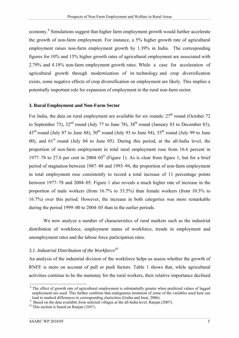
00), and 61st round (July 04 to June 05). During this period, at the all-India level, the

proportion of non-farm employment in total rural employment rose from 16.6 percent in

1977–78 to 27.6 per cent in 2004–059 (Figure 1). As is clear from figure 1, but for a brief

period of stagnation between 1987–88 and 1993–94, the proportion of non-farm employment

in total employment rose consistently to record a total increase of 11 percentage points

between 1977–78 and 2004–05. Figure 1 also reveals a much higher rate of increase in the

proportion of male workers (from 16.7% to 33.5%) than female workers (from 10.3% to

16.7%) over this period. However, the increase in both categories was more remarkable

during the period 1999–00 to 2004–05 than in the earlier periods.

We now analyze a number of characteristics of rural markets such as the industrial

distribution of workforce, employment status of workforce, trends in employment and

unemployment rates and the labour force participation rates.

3.1. Industrial Distribution of the Workforce10

An analysis of the industrial division of the workforce helps us assess whether the growth of

RNFE is more on account of pull or push factors. Table 1 shows that, while agricultural

activities continue to be the mainstay for the rural workers, their relative importance declined

8 The effect of growth rate of agricultural employment is substantially greater when predicted values of lagged

employment are used. This further confirms that endogenous treatment of some of the variables used here can lead to marked differences in corresponding elasticities (Gaiha and Imai, 2006).

9 Based on the data available from selected villages at the all-India level, Ranjan (2007). 10 This section is based on Ranjan (2007).


6 ASARC WP 2010/05

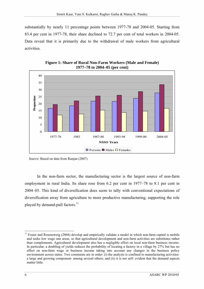
substantially by nearly 11 percentage points between 1977-78 and 2004-05. Starting from

83.4 per cent in 1977-78, their share declined to 72.7 per cent of total workers in 2004-05.

Data reveal that it is primarily due to the withdrawal of male workers from agricultural

activities.

Figure 1: Share of Rural Non-Farm Workers (Male and Female) 1977–78 to 2004–05 (per cent)

0

5

10

15

20

25

30

35

40

1977-78 1983 1987-88 1993-94 1999-00 2004-05

NSSO Years

Prop

ortio

n

Persons Males Females

Source: Based on data from Ranjan (2007)

In the non-farm sector, the manufacturing sector is the largest source of non-farm

employment in rural India. Its share rose from 6.2 per cent in 1977–78 to 8.1 per cent in

2004–05. This kind of diversification does seem to tally with conventional expectations of

diversification away from agriculture to more productive manufacturing, supporting the role

played by demand-pull factors.11

11 Foster and Rosenzweig (2004) develop and empirically validate a model in which non-farm capital is mobile

and seeks low wage rate areas, so that agricultural development and non-farm activities are substitutes rather than complements. Agricultural development also has a negligible effect on local non-farm business income. In particular, a doubling of yields reduces the probability of locating a factory in a village by 27% but has no effect on non-farm wage or business income taking into account any changes in the business policy environment across states. Two comments are in order: (i) the analysis is confined to manufacturing activities- a large and growing component- among several others; and (ii) it is not self- evident that the demand aspects matter little.


ASARC WP 2010/05 7

Table 1: Sectoral Distribution of Workers in Rural India (1977–78 to 2004–05)

Sectors 1977–78 1983 1987–88 1993–94 1999–00 2004–05

Agriculture and Allied 83.4 81.5 78.3 78.4 76.3 72.7

Secondary Sector 8.0 9.0 11.3 10.2 11.4 13.7

Mining and Quarrying 0.4 0.5 0.6 0.6 0.5 0.5

Manufacturing 6.2 6.8 7.2 7.0 7.4 8.1

Electricity, Gas and Water 0.1 0.1 0.2 0.2 0.2 0.2

Construction 1.3 1.6 3.3 2.4 3.3 4.9

Tertiary Sector 8.6 9.4 10.4 11.4 12.4 13.6

Trade, Hotels and Restaurants 3.3 3.4 4.0 4.3 5.1 6.1

Transport & Communication 0.8 1.1 1.3 1.4 2.1 2.5

Other Services 4.5 4.9 5.1 5.7 5.2 5.0

Source: Ranjan (2007).

Till 1999–00, the second largest non-farm employment source was other services

sector. While this includes some modern services, many of these activities are in the nature of

residual opportunities exploited when employment in the commodity producing sectors is not

growing fast enough. The relative share of these services in total employment stood at 5.0 per

cent in 2004–05 compared with 4.5 per cent in 1977–78. However, it is notable that their

employment contribution registered a decline of 0.7 percentage points during the nineties,

from 5.7 per cent in 1993–94 to 5.0 in 2004–05. That is when the proportion of employment

in manufacturing sector was growing, and that of other services was stagnant or declining,

implying a degree of dynamism. The sectors that have experienced a substantial increase in

employment levels over the period 1977–78 to 2004–05 are ‘construction’ (from 1.3% to

4.9%) and ‘trade, hotels and restaurants’ (from 3.3% to 6.1%). On the other hand,

employment shares in rural non-farm activities (RNFA) such as ‘mining and quarrying’ and

‘electricity, gas and water’ are not only low but have remained stagnant over the period

1977–78 to 2004–05.

3.2. Trends in Employment Status of Rural Labour

Employment trends in agriculture and non-agriculture sectors over the period 1977–78 to

2004-05 were dissimilar (Ranjan, 2007). For instance, for the ‘males’, while a decline in self-

employment (from 51.5% to 40.9%) and regular employment (from 4.9% to 0.9%) occurred

in the farm sector, this decline was largely made up by an increase in the self (from 10.5% to


8 ASARC WP 2010/05

15.5%) and casually employed (from 3.8% to 9.5%) in the non-farm sector as well as casual

workers in the agriculture sector (from 16% to 23%). The number of casual workers

increased not only in the non-farm sector, but also in the farm sector implying a growing

casualization of the rural ‘male’ workforce. This evidence of casualization of the rural work

force in the farm sector is of serious concern because the declining incidence of self-

employment is assumed to drive some people out of self-cultivation to add to the ranks of the

landless agricultural laborers.

The trend decline in the self- employment of farm sector was much sharper among the

male than the female workers. The proportion of self-employed male workers in the farm

sector declined by nearly 11 percentage points as compared with 4 percentage points in the

case of female workers. Further, the highest number of workers in the rural areas comprised

self-employed workers, followed by casually employed workers. Only a small proportion

consisted of regularly employed workers. However, the presence of regular workers was

relatively higher in the non-farm sector.

3.3. Trends in Employment and Unemployment Rates in Rural India

Various studies (Ministry of Finance 2004; Planning Commission 2006) in the past few years

have expressed a concern about the growth of employment decelerating or declining in the

post-reform period. Further, using the NSS estimates, Srivastava (2006) states that there has

been a virtual collapse of rural employment. However, Srinivasan (2008) refutes this. He

questions their methodology and offers an alternative set of results summarized below12.

Fitting a simple trend regression to the employment-unemployment data of the NSSO from

the 27th round to the 61st round (i.e. over the period 1972–73 to 2004–05), the following

trends emerge:

Employment Trends

1. For males regardless of the reference period (one year for US, a week for CWS and

person day rate for CDS13) used, there is no statistically significant trend in the rural

employment rate. This is in sharp contrast to the statistically significant upward trend

in the urban male employment rate. The fact that there is a significant upward trend in

12 For a more detailed analysis, see, Srinivasan (2010). 13 US (PS+SS): Usual Status (Principal and Secondary) per 1000 persons; CWS: Current Weekly Status per

1000 persons in the labour force; and CDS: Current Daily Status per 1000 person-days in the labour force. For a careful exposition, see Srinivasan (2010).


ASARC WP 2010/05 9

the employment rate of urban males but not rural males is consistent with the fact that

reforms by and large had no rural components.

2. The employment trend for rural females is negative and significant (US), while no

significant trend exists in the other two measures (CWS and CDS).

Unemployment Trends

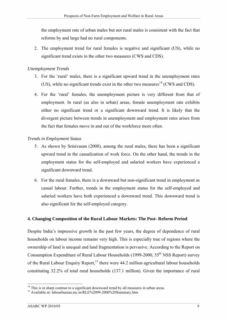
3. For the ‘rural’ males, there is a significant upward trend in the unemployment rates

(US), while no significant trends exist in the other two measures14 (CWS and CDS).

4. For the ‘rural’ females, the unemployment picture is very different from that of

employment. In rural (as also in urban) areas, female unemployment rate exhibits

either no significant trend or a significant downward trend. It is likely that the

divergent picture between trends in unemployment and employment rates arises from

the fact that females move in and out of the workforce more often.

Trends in Employment Status

5. As shown by Srinivasan (2008), among the rural males, there has been a significant

upward trend in the casualization of work force. On the other hand, the trends in the

employment status for the self-employed and salaried workers have experienced a

significant downward trend.

6. For the rural females, there is a downward but non-significant trend in employment as

casual labour. Further, trends in the employment status for the self-employed and

salaried workers have both experienced a downward trend. This downward trend is

also significant for the self-employed category.

4. Changing Composition of the Rural Labour Markets: The Post- Reform Period

Despite India’s impressive growth in the past few years, the degree of dependence of rural

households on labour income remains very high. This is especially true of regions where the

ownership of land is unequal and land fragmentation is pervasive. According to the Report on

Consumption Expenditure of Rural Labour Households (1999-2000, 55th NSS Report) survey

of the Rural Labour Enquiry Report,15 there were 44.2 million agricultural labour households

constituting 32.2% of total rural households (137.1 million). Given the importance of rural

14 This is in sharp contrast to a significant downward trend by all measures in urban areas. 15 Available at: labourbureau.nic.in/RLE%2099-2000%20Summary.htm


10 ASARC WP 2010/05

labour markets, this section focuses on how rural non-farm labour markets have evolved over

time, given the changing macro-economic policies since the 1990s.

4.1. Labour Force Participation Rates in RNFE

Analysis of the 50th (July 1993-June 1994) and 61st (July 2004 — June 2005) rounds reveals

that the average labour force participation rate (LFPR) in rural non-farm sector (usual:

PS+SS) declined marginally — from 44.9 per cent in 1993 to 44.6 percent in 2004 (i.e. a

decline from 449 persons per 1000 persons to 446 persons per 1000 persons over the period

1993 to 2004.16

Trends by Gender: Disaggregation by gender shows that, while the LFPR for females

increased over the period in question, that of males came down. However, despite the fall in

the LFPR of males, they continue to dominate the labour market as their participation rate

(PR: PS+SS) at 55.5 per cent in 2004 is almost double that of the females at 33.3 per cent.

Table 2: Labour Force Participation Rate (per 1000 persons) in Rural India by Gender, 1993–94 to 2004–05

Usual (PS) Usual (PS+SS) CWS

Gender 1993–94 2004–05 1993–94 2004–05 1993–94 2004–05

Male 549 546 561 555 547 545

Female 237 249 330 333 276 287

All 398 401 449 446 415 418

Source: Authors’ calculations

Trends by Age Group: Barring the 30-60 age group, where the LFPR went up by 1.5 per cent

(from 77.2% to 78.4%) over the period 1993 to 2004, the PR fell for all other age groups. The

decline ranged from 2.2 per cent for the 60+ age group to 4 per cent for the 15 to 30 age

group. In 2004, the LFPR was highest for the age group 30 to 60 (78.4), followed by workers

in the 15 to 30 age group (64.4%). The 60 plus age group witnessed a LFPR of 40.3 per cent.

LFPR for children below 15 years was at 0.4 per cent. Similar age-wise distribution is

observed in 1993-94.

16 In reporting participation per thousand persons, we follow Srinivasan (2010).


ASARC WP 2010/05 11

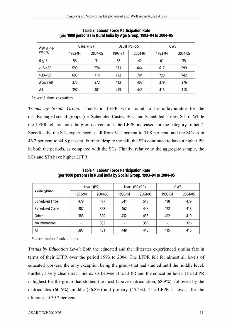
Table 3: Labour Force Participation Rate (per 1000 persons) in Rural India by Age Group, 1993–94 to 2004–05

Usual (PS) Usual (PS+SS) CWS Age group (years) 1993-94 2004-05 1993-94 2004-05 1993-94 2004-05

0-<15 55 31 68 40 61 35

>15-<30 590 574 671 644 617 599

>30-<60 693 714 772 784 720 742

Above 60 375 372 412 403 379 376

All 397 401 449 446 415 418


Trends by Social Group: Trends in LFPR were found to be unfavourable for the

disadvantaged social groups (i.e. Scheduled Castes, SCs, and Scheduled Tribes, STs). While

the LFPR fell for both the groups over time, the LFPR increased for the category ‘others’.

Specifically, the STs experienced a fall from 54.1 percent to 51.8 per cent, and the SCs from

46.2 per cent to 44.8 per cent. Further, despite the fall, the STs continued to have a higher PR

in both the periods, as compared with the SCs. Finally, relative to the aggregate sample, the

SCs and STs have higher LFPR.

Table 4: Labour Force Participation Rate (per 1000 persons) in Rural India by Social Group, 1993–94 to 2004–05

Usual (PS) Usual (PS+SS) CWS Social group

1993-94 2004-05 1993-94 2004-05 1993-94 2004-05

Scheduled Tribe 479 477 541 518 490 479

Scheduled Caste 407 398 462 448 422 418

Others 383 390 432 435 402 410

No information - 302 - 356 - 326

All 397 401 449 446 415 416


Trends by Education Level: Both the educated and the illiterates experienced similar fate in

terms of their LFPR over the period 1993 to 2004. The LFPR fell for almost all levels of

educated workers, the only exception being the group that had studied until the middle level.

Further, a very clear direct link exists between the LFPR and the education level. The LFPR

is highest for the group that studied the most (above matriculation, 68.9%), followed by the

matriculates (60.6%), middle (56.8%) and primary (45.4%). The LFPR is lowest for the

illiterates at 39.2 per cent.


12 ASARC WP 2010/05

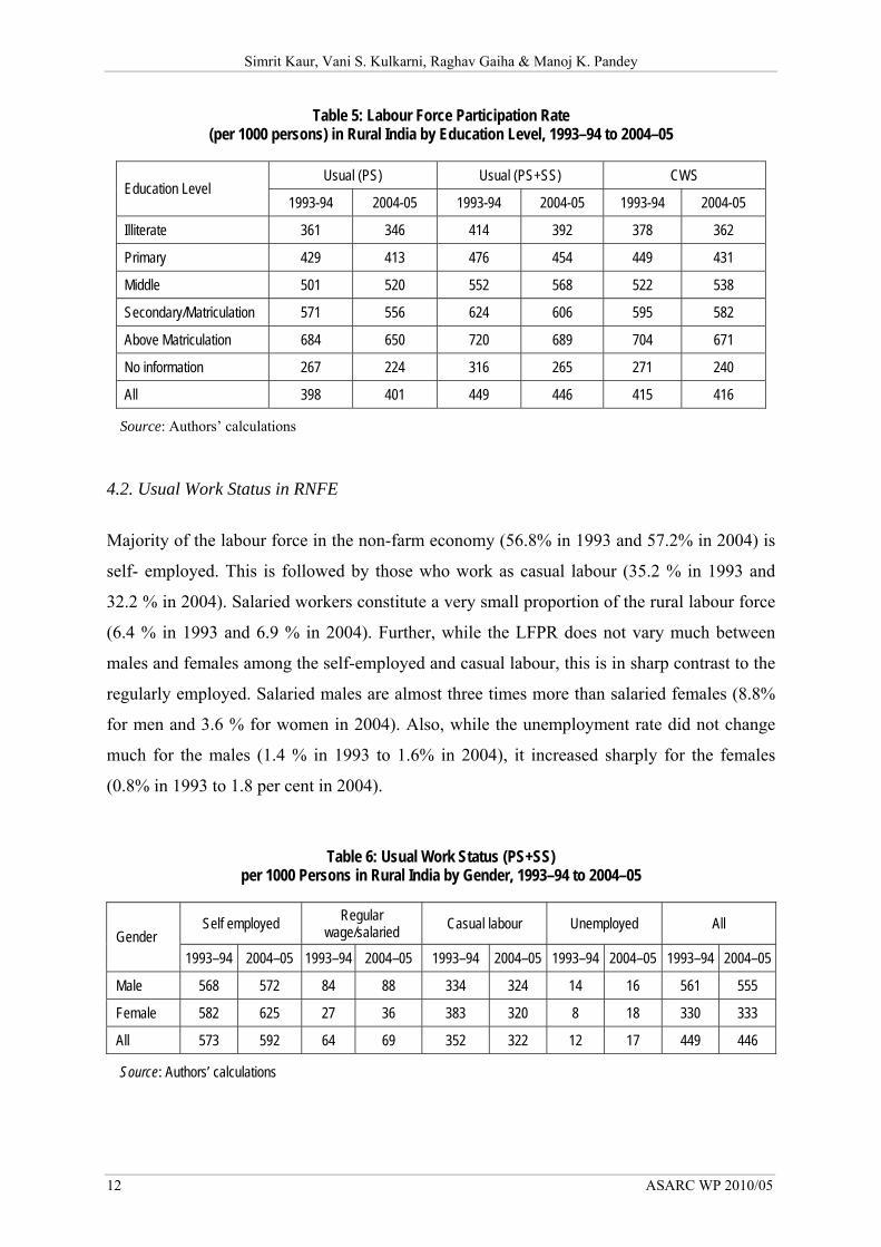
Table 5: Labour Force Participation Rate (per 1000 persons) in Rural India by Education Level, 1993–94 to 2004–05

Usual (PS) Usual (PS+SS) CWS Education Level

1993-94 2004-05 1993-94 2004-05 1993-94 2004-05

Illiterate 361 346 414 392 378 362

Primary 429 413 476 454 449 431

Middle 501 520 552 568 522 538

Secondary/Matriculation 571 556 624 606 595 582

Above Matriculation 684 650 720 689 704 671

No information 267 224 316 265 271 240

All 398 401 449 446 415 416


4.2. Usual Work Status in RNFE

Majority of the labour force in the non-farm economy (56.8% in 1993 and 57.2% in 2004) is

self- employed. This is followed by those who work as casual labour (35.2 % in 1993 and

32.2 % in 2004). Salaried workers constitute a very small proportion of the rural labour force

(6.4 % in 1993 and 6.9 % in 2004). Further, while the LFPR does not vary much between

males and females among the self-employed and casual labour, this is in sharp contrast to the

regularly employed. Salaried males are almost three times more than salaried females (8.8%

for men and 3.6 % for women in 2004). Also, while the unemployment rate did not change

much for the males (1.4 % in 1993 to 1.6% in 2004), it increased sharply for the females

(0.8% in 1993 to 1.8 per cent in 2004).

Table 6: Usual Work Status (PS+SS)

per 1000 Persons in Rural India by Gender, 1993–94 to 2004–05

Self employed Regular wage/salaried Casual labour Unemployed All

Gender 1993–94 2004–05 1993–94 2004–05 1993–94 2004–05 1993–94 2004–05 1993–94 2004–05

Male 568 572 84 88 334 324 14 16 561 555

Female 582 625 27 36 383 320 8 18 330 333

All 573 592 64 69 352 322 12 17 449 446



ASARC WP 2010/05 13

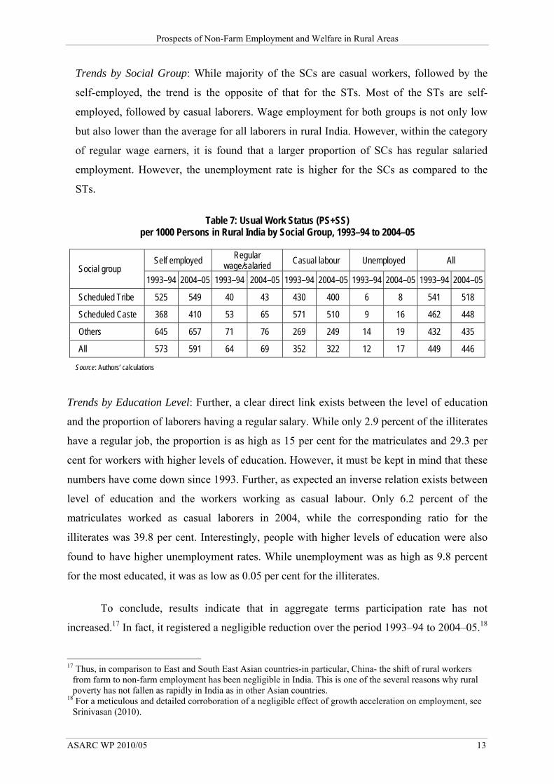
Trends by Social Group: While majority of the SCs are casual workers, followed by the

self-employed, the trend is the opposite of that for the STs. Most of the STs are self-

employed, followed by casual laborers. Wage employment for both groups is not only low

but also lower than the average for all laborers in rural India. However, within the category

of regular wage earners, it is found that a larger proportion of SCs has regular salaried

employment. However, the unemployment rate is higher for the SCs as compared to the

STs.


per 1000 Persons in Rural India by Social Group, 1993–94 to 2004–05

Self employed Regular wage/salaried Casual labour Unemployed All

Social group 1993–94 2004–05 1993–94 2004–05 1993–94 2004–05 1993–94 2004–05 1993–94 2004–05

Scheduled Tribe 525 549 40 43 430 400 6 8 541 518

Scheduled Caste 368 410 53 65 571 510 9 16 462 448

Others 645 657 71 76 269 249 14 19 432 435

All 573 591 64 69 352 322 12 17 449 446


Trends by Education Level: Further, a clear direct link exists between the level of education

and the proportion of laborers having a regular salary. While only 2.9 percent of the illiterates

have a regular job, the proportion is as high as 15 per cent for the matriculates and 29.3 per

cent for workers with higher levels of education. However, it must be kept in mind that these

numbers have come down since 1993. Further, as expected an inverse relation exists between

level of education and the workers working as casual labour. Only 6.2 percent of the

matriculates worked as casual laborers in 2004, while the corresponding ratio for the

illiterates was 39.8 per cent. Interestingly, people with higher levels of education were also

found to have higher unemployment rates. While unemployment was as high as 9.8 percent

for the most educated, it was as low as 0.05 per cent for the illiterates.

To conclude, results indicate that in aggregate terms participation rate has not

increased.17 In fact, it registered a negligible reduction over the period 1993–94 to 2004–05.18

17 Thus, in comparison to East and South East Asian countries-in particular, China- the shift of rural workers

from farm to non-farm employment has been negligible in India. This is one of the several reasons why rural poverty has not fallen as rapidly in India as in other Asian countries.

18 For a meticulous and detailed corroboration of a negligible effect of growth acceleration on employment, see Srinivasan (2010).


14 ASARC WP 2010/05

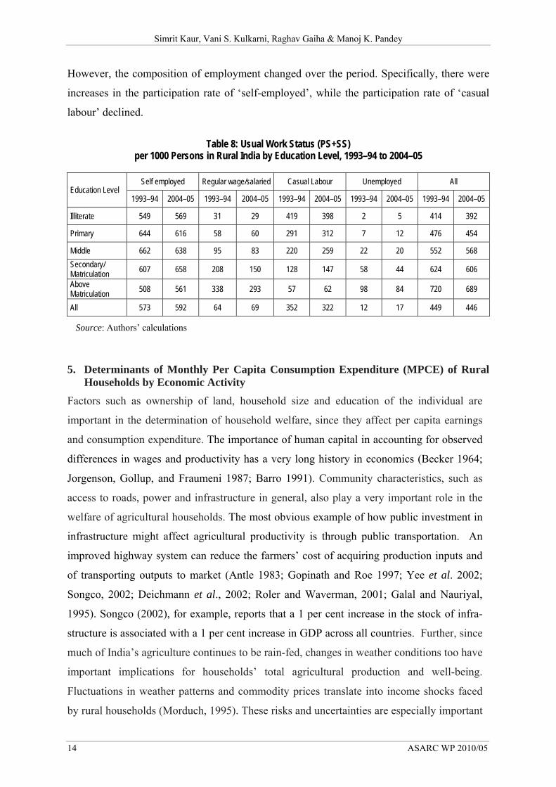
However, the composition of employment changed over the period. Specifically, there were

increases in the participation rate of ‘self-employed’, while the participation rate of ‘casual

labour’ declined.


per 1000 Persons in Rural India by Education Level, 1993–94 to 2004–05

Self employed Regular wage/salaried Casual Labour Unemployed All Education Level

1993–94 2004–05 1993–94 2004–05 1993–94 2004–05 1993–94 2004–05 1993–94 2004–05

Illiterate 549 569 31 29 419 398 2 5 414 392

Primary 644 616 58 60 291 312 7 12 476 454

Middle 662 638 95 83 220 259 22 20 552 568 Secondary/ Matriculation 607 658 208 150 128 147 58 44 624 606

Above Matriculation 508 561 338 293 57 62 98 84 720 689

All 573 592 64 69 352 322 12 17 449 446


5. Determinants of Monthly Per Capita Consumption Expenditure (MPCE) of Rural Households by Economic Activity

Factors such as ownership of land, household size and education of the individual are

important in the determination of household welfare, since they affect per capita earnings

and consumption expenditure. The importance of human capital in accounting for observed

differences in wages and productivity has a very long history in economics (Becker 1964;

Jorgenson, Gollup, and Fraumeni 1987; Barro 1991). Community characteristics, such as

access to roads, power and infrastructure in general, also play a very important role in the

welfare of agricultural households. The most obvious example of how public investment in

infrastructure might affect agricultural productivity is through public transportation. An

improved highway system can reduce the farmers’ cost of acquiring production inputs and

of transporting outputs to market (Antle 1983; Gopinath and Roe 1997; Yee et al. 2002;

Songco, 2002; Deichmann et al., 2002; Roler and Waverman, 2001; Galal and Nauriyal,

1995). Songco (2002), for example, reports that a 1 per cent increase in the stock of infra-

structure is associated with a 1 per cent increase in GDP across all countries. Further, since

much of India’s agriculture continues to be rain-fed, changes in weather conditions too have

important implications for households’ total agricultural production and well-being.

Fluctuations in weather patterns and commodity prices translate into income shocks faced

by rural households (Morduch, 1995). These risks and uncertainties are especially important


ASARC WP 2010/05 15

as they result in consumption fluctuations (Dercon, 1996, Paxon, 1992). While rainfall

variability is not the only exogenous factor affecting farm output, it contributes significantly

to income variability and consequently welfare (Rosenzweig and Binswanger, 1993).

Gaiha and Imai (2004) and Gaiha et al. (2009) examine the effect of droughts on

household welfare. They state that loss of agricultural output and food shortage are not the

only consequences of droughts. There are often large second round effects some of which

persist over time. By the time these effects play out, the overall economic loss is

substantially greater than the first round loss of income. Hardships manifest in malnutrition,

poverty, disinvestment in human capital (e.g. withdrawal of children from school),

liquidation of assets (e.g. sale of livestock) with impairment of future economic prospects,

and, in extreme cases, mortality.19 Given the importance of rainfall variability on economic

well-being, in the analysis that follows, rainfall fluctuations along with education and

infrastructure have been incorporated as explanatory variables to analyze their impact on

consumption expenditure of rural households in India.

The Model

Here the relationship between log of monthly per capita consumption expenditure, on the one

hand, and individual, household and village level characteristics, on the other, is explored for

‘all rural households’, ‘self employed in non-agriculture’, ‘agricultural laborers’, ‘other

laborers’ and ‘self employed in agriculture’, based on regression analysis of the 61st round of

the NSS.20

The model is specified as below:

Qi = α0 + α1Hi + α3Ii +α4Si + θi

where

• Qi is the log of monthly per capita consumption expenditure (MPCE).

• Hi is a vector of individual characteristics such as gender and educational status of

each person, and household characteristics such as size of the household and caste to

which each person belongs. A households endowments include land holding.

• Ii is a vector of community level infrastructure characteristics (both physical and

financial) such as access to finance and roads.

19 Responses to such risks can occur at two stages. One takes place prior to the occurrence of the event (i.e. risk

reduction) and the second after the event (i.e. risk mitigation). See, for example, Mpuga and Okwi, 2002; Dercon, 1996; Morduch, 1995; Townsend, 1995; and Paxson, 1992.

20 The results based on the 55th round of the NSS are not reported except some key elasticities for comparison with those obtained from the 61st round of the NSS.


16 ASARC WP 2010/05

• Si is a variable designed to capture shock experienced by households due to

fluctuations in rainfall. The rainfall shock is measured as normalized rainfall-

deviation of actual annual rainfall (2004-05 for 61st round) from its mean over the

period 1970 to 2005, divided by its standard deviation.21 For the regression, a dummy

for normalized rainfall for the year 2004–05 has been used. It takes the value 1if normalized

rainfall exceeds 0 and 0 otherwise.

• θi is the random error term assumed to be independently and identically (i.i.d.)

distributed with constant variance.

Data Sources

Data sources for the household level characteristics are primarily based on the 61st (July 2004

to June 2005) round of survey conducted by the National Sample Survey Organisation

(NSSO) on employment and unemployment in India.22 For rural India, 8128 villages formed

the Central sample for this round. Of these, 7999 villages were eventually surveyed. The

total number of households is 398,031. Data pertaining to ‘Infrastructure’ variable is taken

from The Rural Infrastructure Report, 2007, published by the National Council of Applied

Economic Research (NCAER). Data on rainfall were collected from the India Meteorological

Department. Local area rainfall data — obtained from 38 weather stations across the country

— are merged with the household survey data for the respective years.

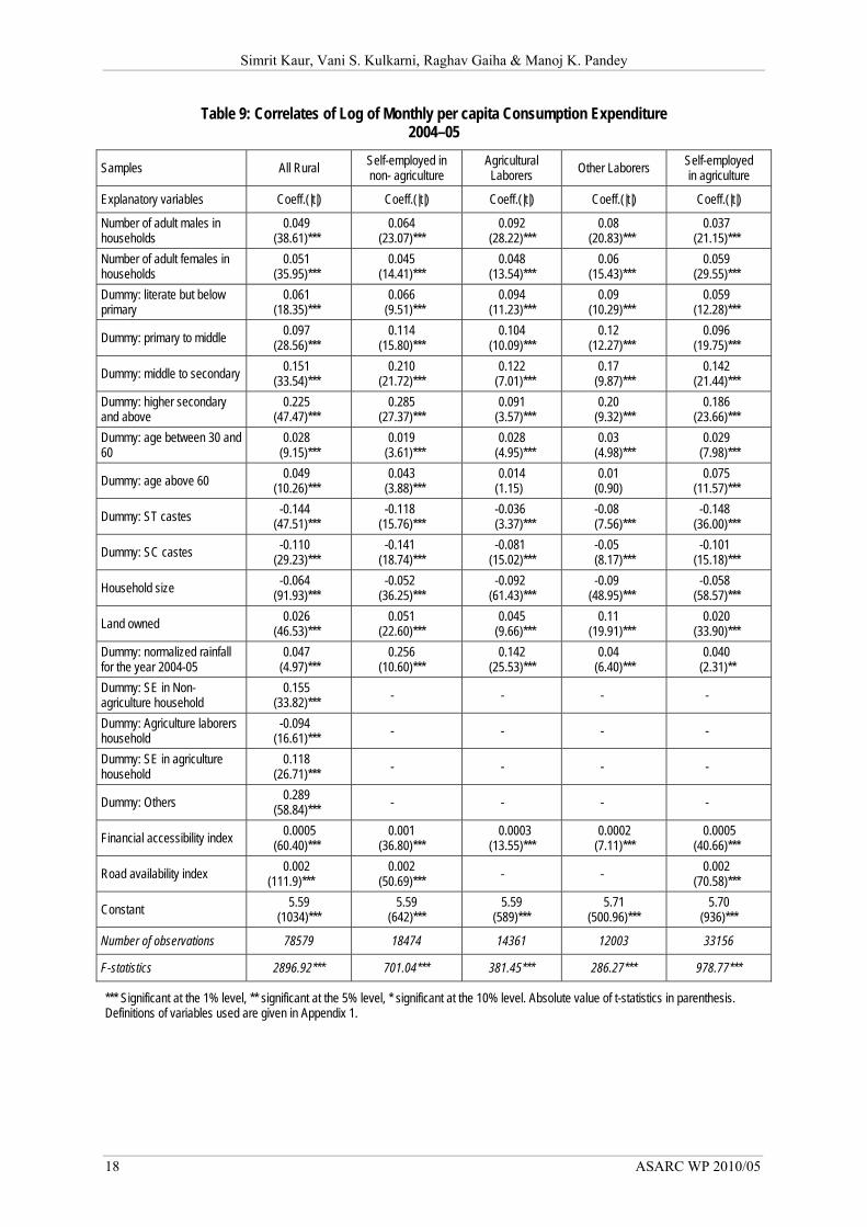
Results

The results are summarized in Table 9. Let us first consider the association between

household characteristics and welfare across farm and non-farm activities.

• The higher the number of adult males, the greater is the welfare-especially among

‘labour households’. So also is the case with number of adult females but with

relatively large contributions to welfare in ‘other labour’ and ‘self-employed in

agriculture’ households.

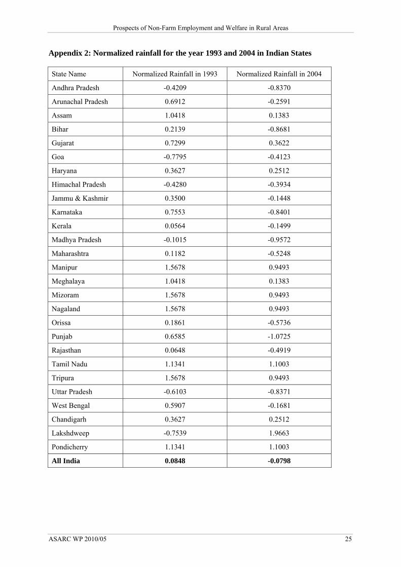
21 As suggested by the reviewer, we tried to use the normalized rainfall and its square (the latter is posited to

capture the adverse effects of excess deficit or surplus rainfall, through crop yields and related activities, on the welfare indicator) for our regression analysis. However, as the results were implausible (e.g. negative expenditure-rainfall elasticities in most cases), we decided to rely on our specification despite its limitations (e.g. it does not distinguish between moderate or more than moderate rainfall in the excess over normal rain-fall). Also, state level averages of actual rainfall sometimes conceal large variation in rainfall within a state. So a more definitive assessment of expenditure-rainfall elasticities is not feasible with the data at our disposal. For details of state-wise distribution of normalized rainfall (1993–94 and 2004–05), refer to appendix 2.

22 A stratified multi-stage design was adopted for the 61st round survey. Agriculture and farm activities, and non-agriculture and non-farm activities are synonymously used.


ASARC WP 2010/05 17

• Welfare and household size are inversely related, more so among the ‘labour

households’.

• Education contributes across all types of households. The pattern of welfare effects is,

however, somewhat surprising. Relative to illiterates, the progression from Primary to

Higher secondary and above is generally associated with larger contributions to

welfare across different types of households. While the ‘self-employed in non-

agriculture’ benefit most from higher secondary and above levels of education, ‘other

labourers’ and ‘self-employed in agriculture’ also benefit substantially.

• Whether the human capital embodied in work-experience and learning- by- doing

matter is confirmed through age-group as a proxy. Both among the ‘self-employed’ in

non-farm and farm activities are observed to benefit more from older workers.

• As expected, other things being equal, the SC and ST households have lower welfare,

regardless of the type of households, relative to others.

• The association of welfare with amount of land holding reveals a somewhat surprising

pattern — benefits to ‘other labour’, ‘self-employed in non-farm’ activities and

‘agriculture labour’ households vary in this order.

We now examine the association between infrastructure, rainfall and welfare across farm and

non-farm activities.

• Infrastructure matters a great deal with both roads and financial services contributing

to welfare across all household groups. While financial services enhance welfare of

all types of households, roads benefit ‘self-employed in non-agriculture and

agriculture’. It is also interesting to note that financial services benefit all types of

households but the effects are small.

• Household welfare varies with normalised rainfall across all types of households, with

the highest positive effect on the welfare of ‘self-employed in non-agriculture’,

followed by ‘agricultural labour’ households. The strong association of positive

rainfall shocks with the welfare of ‘self-employed in non-agriculture’ is indicative of

strong linkages with agriculture.

• In the column for ‘all rural households’, the dummies for different types of

households suggest that ‘others’ had the highest welfare indicator (presumably

because of the preponderance of salaried households), followed by ‘self-employed in

non-agriculture’, and then ‘self-employed in agriculture’. The lowest rung belongs to

‘agricultural labour households’.


18 ASARC WP 2010/05

Table 9: Correlates of Log of Monthly per capita Consumption Expenditure 2004–05

Samples All Rural Self-employed in non- agriculture

Agricultural Laborers Other Laborers Self-employed

in agriculture

Explanatory variables Coeff.(|t|) Coeff.(|t|) Coeff.(|t|) Coeff.(|t|) Coeff.(|t|)

Number of adult males in households

0.049 (38.61)***

0.064 (23.07)***

0.092 (28.22)***

0.08 (20.83)***

0.037 (21.15)***

Number of adult females in households

0.051 (35.95)***

0.045 (14.41)***

0.048 (13.54)***

0.06 (15.43)***

0.059 (29.55)***

Dummy: literate but below primary

0.061 (18.35)***

0.066 (9.51)***

0.094 (11.23)***

0.09 (10.29)***

0.059 (12.28)***

Dummy: primary to middle 0.097 (28.56)***

0.114 (15.80)***

0.104 (10.09)***

0.12 (12.27)***

0.096 (19.75)***

Dummy: middle to secondary 0.151 (33.54)***

0.210 (21.72)***

0.122 (7.01)***

0.17 (9.87)***

0.142 (21.44)***

Dummy: higher secondary and above

0.225 (47.47)***

0.285 (27.37)***

0.091 (3.57)***

0.20 (9.32)***

0.186 (23.66)***

Dummy: age between 30 and 60

0.028 (9.15)***

0.019 (3.61)***

0.028 (4.95)***

0.03 (4.98)***

0.029 (7.98)***

Dummy: age above 60 0.049 (10.26)***

0.043 (3.88)***

0.014 (1.15)

0.01 (0.90)

0.075 (11.57)***

Dummy: ST castes -0.144 (47.51)***

-0.118 (15.76)***

-0.036 (3.37)***

-0.08 (7.56)***

-0.148 (36.00)***

Dummy: SC castes -0.110 (29.23)***

-0.141 (18.74)***

-0.081 (15.02)***

-0.05 (8.17)***

-0.101 (15.18)***

Household size -0.064 (91.93)***

-0.052 (36.25)***

-0.092 (61.43)***

-0.09 (48.95)***

-0.058 (58.57)***

Land owned 0.026 (46.53)***

0.051 (22.60)***

0.045 (9.66)***

0.11 (19.91)***

0.020 (33.90)***

Dummy: normalized rainfall for the year 2004-05

0.047 (4.97)***

0.256 (10.60)***

0.142 (25.53)***

0.04 (6.40)***

0.040 (2.31)**

Dummy: SE in Non-agriculture household

0.155 (33.82)*** - - - -

Dummy: Agriculture laborers household

-0.094 (16.61)*** - - - -

Dummy: SE in agriculture household

0.118 (26.71)*** - - - -

Dummy: Others 0.289 (58.84)*** - - - -

Financial accessibility index 0.0005 (60.40)***

0.001 (36.80)***

0.0003 (13.55)***

0.0002 (7.11)***

0.0005 (40.66)***

Road availability index 0.002 (111.9)***

0.002 (50.69)*** - - 0.002

(70.58)***

Constant 5.59 (1034)***

5.59 (642)***

5.59 (589)***

5.71 (500.96)***

5.70 (936)***

Number of observations 78579 18474 14361 12003 33156

F-statistics 2896.92*** 701.04*** 381.45*** 286.27*** 978.77***

*** Significant at the 1% level, ** significant at the 5% level, * significant at the 10% level. Absolute value of t-statistics in parenthesis. Definitions of variables used are given in Appendix 1.


ASARC WP 2010/05 19

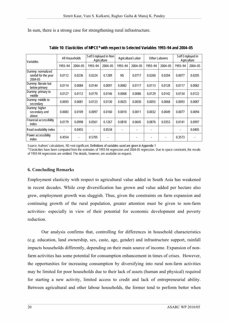
A somewhat surprising result is the substantially higher elasticity of expenditure for the ‘self-

employed in non-farm’ activities to rainfall over the period 1993–2004 (table 10). Whether

this is because of stronger farm and non-farm linkages requires further investigation. The

expenditure elasticities with respect to education also reveal a pattern which is partly

surprising.

• Expenditure-education elasticities are significant for each type of household and for

all in both 1993 and 2004.

• However, in most cases, the magnitudes are small.

• In most cases, the elasticities rise from below primary to primary-middle. Higher

levels of education, with a few exceptions, are, however, associated with lower

expenditure elasticities. Presumably, this finding reflects limited employment

opportunities for those with higher educational attainments.

• Over the period 1993–2004, and in most cases, the expenditure elasticities decreased

across different education levels and types of households. A somewhat surprising

finding is that expenditure elasticities were higher for ‘agricultural labour’ and ‘other

labour’ households. Also, for the highest level of education (i.e. higher secondary and

above), the elasticities were higher for ‘all households’, ‘self-employed in non-

agriculture’, ‘other labourers’ and ‘self employed in agriculture’ in 2004 than in 1993.

In sum, higher school level education contributes to welfare.

That rural infrastructure matters in enhancing welfare is also confirmed by our analysis.

Specifically,

• Financial access is associated with significantly higher welfare across all and different

types of households. Also, the elasticities were higher for ‘all households’, ‘self

employed in non-agriculture’, and for ‘self employed in agriculture’, and lower for

both ‘agriculture’ and ‘other labour’ households. Finally, with a few exceptions, these

elasticities were higher in 2004.

• Road availability also contributes significantly to welfare of ‘all households’, ‘self

employed in non-agriculture’, and ‘self employed in agriculture’ in 2004.23

• Power accessibility seems to matter most, going by the expenditure elasticities for

1993.24

23 The estimates for 1993 are not reported as these were not robust. 24 As power accessibility was highly collinear with other infrastructure variables in 2004, it was omitted.

Consequently, the coefficients of road and finance are likely to be biased upward.


20 ASARC WP 2010/05

In sum, there is a strong case for strengthening rural infrastructure.

Table 10: Elasticities of MPCE* with respect to Selected Variables 1993–94 and 2004–05

All Households Self Employed in Non Agriculture Agricultural Labor Other Laborers Self Employed in

Agriculture Variables 1993–94 2004–05 1993–94 2004–05 1993–94 2004–05 1993–94 2004–05 1993–94 2004–05

Dummy: normalized rainfall for the year 2004-05

0.0112 0.0236 0.0224 0.1289 NS 0.0717 0.0260 0.0204 0.0077 0.0205

Dummy: literate but below primary 0.0114 0.0084 0.0144 0.0097 0.0082 0.0117 0.0113 0.0128 0.0117 0.0082

Dummy: primary to middle 0.0127 0.0112 0.0170 0.0146 0.0068 0.0086 0.0129 0.0142 0.0134 0.0122

Dummy: middle to secondary 0.0093 0.0081 0.0123 0.0130 0.0025 0.0030 0.0055 0.0068 0.0093 0.0087

Dummy: higher secondary and above

0.0083 0.0109 0.0097 0.0160 0.0010 0.0011 0.0032 0.0049 0.0077 0.0094

Financial accessibility index 0.0179 0.0998 0.0561 0.1267 0.0818 0.0645 0.0876 0.0353 0.0141 0.0997

Road availability index - 0.0455 - 0.0534 - - - - 0.0405 Power accessibility

index 0.4554 - 0.5705 - - - - 0.3573 -

Source: Authors’ calculations. NS=not significant. Definitions of variables used are given in Appendix 1 * Elasticities have been computed from the estimates of 1993-94 regression and 2004-05 regression. Due to space constraint, the results of 1993-94 regressions are omitted. The details, however, are available on request.

6. Concluding Remarks

Employment elasticity with respect to agricultural value added in South Asia has weakened

in recent decades. While crop diversification has grown and value added per hectare also

grew, employment growth was sluggish. Thus, given the constraints on farm expansion and

continuing growth of the rural population, greater attention must be given to non-farm

activities- especially in view of their potential for economic development and poverty

reduction.

Our analysis confirms that, controlling for differences in household characteristics

(e.g. education, land ownership, sex, caste, age, gender) and infrastructure support, rainfall

impacts households differently, depending on their main source of income. Expansion of non-

farm activities has some potential for consumption enhancement in times of crises. However,

the opportunities for increasing consumption by diversifying into rural non-farm activities

may be limited for poor households due to their lack of assets (human and physical) required

for starting a new activity, limited access to credit and lack of entrepreneurial ability.

Between agricultural and other labour households, the former tend to perform better when


ASARC WP 2010/05 21

rainfall is above normal. A somewhat surprising result is the substantially higher elasticity of

expenditure of both ‘self-employed’ in non-farm and farm activities to rainfall in 2004

relative to 1993. Whether these significantly higher elasticities reflect stronger farm and non-

farm linkages and expansion of agriculture in arid and semi-arid conditions requires further

investigation.

In conclusion, there is strong evidence favoring the growing importance of non-farm

activities. However, resilience of not just farm but also non-farm activities to rainfall shocks

is a major policy imperative.

*********


22 ASARC WP 2010/05

References de Janvry, Alain,E. Sadoulet,, and Nong Zhu (2005), The Role of Non-Farm Incomes in Reducing Rural

Poverty and Inequality in China, UC Berkeley Department of Agricultural and Resource Economics, UCB. CUDARE Working Paper No. 1001. Retrieved from: http://escholarship.org/uc/item/7ts2z766

Antle, John. (1983), ‘Infrastructure and Aggregate Agricultural Productivity: International Evidence’, Economic Development and Cultural Change 31: 609–19.

Barro, Robert J. (1991), ‘Human Capital and Growth in Cross-Country Regressions’, Quarterly Journal of Economics, 106(2, May): 407–443

Becker, Gary S.(1964), Human Capital: A Theoretical and Empirical Analysis, with Special Reference to Education, Columbia University Press.

Deichmann, Uwe, Marianne Fay, Jun Koo and Somik V. Lall. (2002), ‘Economic Structure, Productivity and Infrastructure Quality in Southern Mexico’, World Bank Policy Research Paper No. 2900, October.

Dercon, S. (1996), ‘Risk, crop choice, and savings: Evidence from Tanzania’. Economic Development and Cultural Change, 44(3): 485–513.

Eswaran, M. Kotwal,A., Ramaswami B, and W. Wadhwa (2008). ‘How Does Poverty Decline? Suggestive Evidence from India, 1983–1999’, Cambridge: MA, BREAD Policy Paper No. 014, February 2008.

Foster, A. and M. Rosenzweig (2004), ‘Agricultural Productivity Growth, Rural Economic Diversity and Economic Reforms: India 1970-2000’, Economic Development and Cultural Change, 52: 509–542.

Gaiha, Raghav and Katsushi Imai (2004). ‘Vulnerability, Shocks and Persistence of Poverty - Estimates for Semi-Arid Rural South India’, Oxford Development Studies, 32(2): 261–81.

Gaiha, Raghav and Katsushi Imai (2008), ‘Agricultural Growth, Employment and Wage Rates in Developing Countries’, in G. Kochendorfer-Lucius and B. Pleskovic (eds) Agriculture and Development, Washington DC: World Bank.

Gaiha, Raghav and Katsushi Imai (2007), Non Agricultural Employment and Poverty in India — An Analysis Based on the 60th Round of NSS, Economics Discussion Paper EDP-0705, The University of Manchester.

Gaiha, Raghav, K. Hill, S. Mathur and Vani S. Kulkarni (2009), ‘On Devastating Droughts’, A paper presented at the NBER Conference on Climate Change: Past and Present, Cambridge, MA.

Gopinath, Munisamy and Terry Roe (1997), ‘Sources of Sectoral Growth in an Economy Wide Context: The Case of U.S. Agriculture’, Journal of Productivity Analysis 8, pp. 293-310.

Galal, Ahmed and Bharat Nauriyal. (1995), ‘Evaluation of Rural Road Rehabilitation in Ghana’, Washington DC: Operations Evaluation Department, World Bank.

Government of India (2000), Labour Bureau’s Rural Labour Enquiry Report on Consumption Expenditure of Rural Labour Households, Year 1999–2000 (55th NSS Round) Available at: http://labourbureau.nic.in/RLE%2099-2000%20Summary.htm

GOI (2006), National Sample Survey Organization, Employment-Unemployment Situation in India, Report No. 515, 61st Round (July 2004–June 2005).

Haggblade S, Hazell Peter and T. Reardon (2007), Transforming the Rural Non farm Economy: Opportunities and Threats in the Developing World, Oxford University Press, New Delhi.

Hossain, M. (2004), ‘Rural Non Farm Economy in Bangladesh: A View from Household Surveys’, Centre for Policy Dialogue, Occasional Paper Series 40. Dhaka: Centre for Policy Dialogue.

Jorgenson, Dale W., F. Gollop and B.M. Fraumeni (1987). Productivity and US Economic Growth. Harvard University Press, Cambridge, MA.

Lanjouw, J. and P. Lanjouw (2001), ‘The Rural Non Farm Sector: Issues and Evidence from Developing Countries’, Agricultural Economics 26 (2001) 1–23.

Lanjouw Peter and Rinku Murgai (2008), ‘Poverty Decline, Agricultural Wages, and Non-Farm Employment in Rural India 1983–2004’, Washington DC: The World Bank Policy Research Working Paper 4858, March 2008.

Lanjouw, P. and A. Shariff (2004), ‘Rural Non-Farm Employment in India: Access, Incomes and Poverty Impact’, Economic and Political Weekly 39(40): 4429–46.


ASARC WP 2010/05 23

MOF (2004), Economic Survey 2003–04, New Delhi, Ministry of Finance, Government of India.

Morduch, J. (1995), ‘Income Smoothing and Consumption Smoothing’, Journal of Economic Perspectives, 9(3): 103–14.

Mpuga, P. and P. Okwi. (2002), ‘Why Do Households Save? Analysis Using the Household Survey Data for Uganda’, Final research report submitted to the African Economic Research Consortium, Nairobi, Kenya, December.

Paxson, H.C. (1992), ‘Using Weather Variability to Estimate the Response of Savings to Transitory Income in Thailand’, American Economic Review, 82(1, March): 15–33.

Planning Commission (2006), ‘Towards Faster and More Inclusive Growth: An Approach to the 11th Five Year Plan,’ New Delhi, Planning Commission.

Ranjan, Sharad (2007), Determinants of Rural Non-Farm Employment: An Assessment Based on Village Studies in Western Uttar Pradesh, Unpublished PhD Thesis, Jawaharlal Nehru University.

Reardon, T (1997), ‘Using Evidence of Household Income Diversification to Inform Study of the Rural Non Farm Labour Market in Africa’, World Development 25(5): 735–47.

Reardon, T., K. Stamolous, A. Balisacan, M.E. Cruz, J. Berdegue and B. Banks (1998), ‘Rural Non Farm Income in Developing Countries’, in State of Food and Agriculture, 1998, Special Chapter, Rome: Food and Agricultural Organization of the United Nations.

Reardon T and C.P. Timmer (2007), ‘Transformation of Markets for Agricultural Output in Developing Countries since 1950. How has Thinking Changed?’ in Handbook of Agricultural Economics, R. Evenson and P. Pingail (eds), Volume 3 A, Amsterdam, North Holland.

Roller, Lars Hendrik and Leonard Waverman (2001), ‘Telecommunication Infrastructure and Economic Development: A Simultaneous Approach’, American Economic Review, 91(4), September.

Rosenzweig, R.M. and H.P. Binswanger (1993), ‘Wealth, Weather Risk and the Composition of Profitability of Agricultural Investments’, The Economic Journal, 103(416, January): 56–78.

Saxena, N.C. (2003), ‘The Rural Non-Farm Economy in India: Some Policy Issues, Rural Non-Farm Economy and Livelihood Enhancement’, DFID-World Bank Collaborative Research Project, National Resource Institute, NRI Report No: 2752

Songco, Jocelyn A. (2002), ‘Do Rural Infrastructure Investment Benefit the Poor? A Global View, A Focus on Vietnam’, World Bank Policy Research Working Paper N0. 2796. World Bank, Washington DC.

Srinivasan, T.N. (2008), ‘Employment and Unemployment Since the Early 1970s’, India Development Report, pp.54-70, New Delhi: Oxford University Press.

Srinivasan, T.N. (2010), Employment and India’s development and reforms, Journal of Comparative Economics, (2010), doi:10.1016/j.jce.2009.11.001, in press.

Srivastava, R.S. (2006), ‘Trends in Rural Employment in India with Special Reference to

Agricultural Employment’, in the World Bank’s India Employment Report.

Townsend, M.R. (1995), ‘Consumption Insurance: An Evaluation of Risk-Bearing Systems in Low-Income Economies’, Journal of Economic Perspectives, 9(3): 32–102.

Unni, J. and G. Ravendran (2007), ‘Growth of Employment (1993–2004/5): Illusion of Inclusiveness?’ Economic and Political Weekly, January 20, 2007.

Yee, Jet, Wallace Huffman, Mary Ahearn, and Doris Newton.(2002), ‘Sources of Agricultural Productivity Growth at the State Level, 1960-1993’, in V.E. Ball and G.W. Norton (eds) Agricultural Productivity: Measurement and Sources of Growth, Norwell, MA: Kluwer.: 185-210.


24 ASARC WP 2010/05

Appendix 1: Definitions of Variables Used in the Analysis

Variable Definitions

Number of adult males in households Number of male aged 15 years and above

Number of adult females in households Number of female aged 15 years and above Dummy: age below 30 (reference category) =1 if age of individual<=30 years; 0 otherwise

Dummy: age between 30 and 60 =1 if age of individual>30 and <=60 years; 0 otherwise

Dummy: age above 60 =1 if age of individual>60 years; 0 otherwise

Dummy: illiterate (reference) =1 if illiterate; 0 otherwise

Dummy: literate but below primary =1 if educated but below primary; 0 otherwise

Dummy: primary to middle =1 if passed primary to middle; 0 otherwise

Dummy: middle to secondary =1 if passed middle to secondary; 0 otherwise

Dummy: higher secondary and above =1 if higher secondary and above; 0 otherwise Dummy: other castes (reference category) =1 if social group is OBC and others; 0 otherwise

Dummy: ST castes =1 if social group is ST; 0 otherwise

Dummy: SC castes =1 if social group is SC; 0 otherwise

Household size Household Size

Land owned Land owned by household (in hectares) Dummy: normalized rainfall for the year 2004-05 =1 if normalized rainfall exceeds 0; 0 otherwise

Dummy: SE in Non-agriculture household

=1 if household is self-employed in non-agriculture; 0 if agricultural labour, or other labour3, or self-employed in agriculture or any other hhtype

Dummy: Agriculture laborers household =1 if household is agricultural labour; 0 otherwise

Dummy: SE in agriculture household =1 if household is self-employed in agriculture; 0 otherwise

Dummy: other laborers household (reference) =1 if household is other labours; 0 otherwise

Dummy: others household =1 if household is others type; 0 otherwise

Financial accessibility index Financial allocation composite index for year 1997 or 1993

Road availability index Road availability Index for year 1997 or 1993

Power accessibility index Power accessibility index for year 1997 or 1993


ASARC WP 2010/05 25

Appendix 2: Normalized rainfall for the year 1993 and 2004 in Indian States State Name Normalized Rainfall in 1993 Normalized Rainfall in 2004

Andhra Pradesh -0.4209 -0.8370

Arunachal Pradesh 0.6912 -0.2591

Assam 1.0418 0.1383

Bihar 0.2139 -0.8681

Gujarat 0.7299 0.3622

Goa -0.7795 -0.4123

Haryana 0.3627 0.2512

Himachal Pradesh -0.4280 -0.3934

Jammu & Kashmir 0.3500 -0.1448

Karnataka 0.7553 -0.8401

Kerala 0.0564 -0.1499

Madhya Pradesh -0.1015 -0.9572

Maharashtra 0.1182 -0.5248

Manipur 1.5678 0.9493

Meghalaya 1.0418 0.1383

Mizoram 1.5678 0.9493

Nagaland 1.5678 0.9493

Orissa 0.1861 -0.5736

Punjab 0.6585 -1.0725

Rajasthan 0.0648 -0.4919

Tamil Nadu 1.1341 1.1003

Tripura 1.5678 0.9493

Uttar Pradesh -0.6103 -0.8371

West Bengal 0.5907 -0.1681

Chandigarh 0.3627 0.2512

Lakshdweep -0.7539 1.9663

Pondicherry 1.1341 1.1003

All India 0.0848 -0.0798

prospects of non-farm employment and welfare in rural areas1

Documents