project report - eth z · matlab . project report . agent-based financial ... we hereby agree to...

Lecture with Computer Exercises: Modelling and Simulating Social Systems with

MATLAB

Project Report

Agent-based Financial Markets Model A new approach incorporating findings from the financial crisis

Florian Müller-Reiter Matthias Wyss

Zürich December 2010

of 40

Eigenständigkeitserklärung Hiermit erkläre ich, dass ich diese Gruppenarbeit selbständig verfasst habe, keine anderen als die angegebenen Quellen-Hilfsmittel verwenden habe, und alle Stellen, die wörtlich oder sinngemäß aus veröffentlichen Schriften entnommen wurden, als solche kenntlich gemacht habe. Darüber hinaus erkläre ich, dass diese Gruppenarbeit nicht, auch nicht auszugsweise, bereits für andere Prüfung ausgefertigt wurde.


of 40

Agreement for free-download

We hereby agree to make our source code of this project freely available for download from the web pages of the SOMS chair. Furthermore, we assure that all source code is written by ourselves and is not violating any copyright restrictions.


of 40

Table of content

AGREEMENT FOR FREE-DOWNLOAD 3

TABLE OF CONTENT 4

1. INDIVIDUAL CONTRIBUTIONS 5

2. INTRODUCTION AND MOTIVATIONS 5

3. DESCRIPTION OF THE MODEL 6

4. IMPLEMENTATION 6

4.1. THE AGENT-BASED FINANCIAL MARKET MODEL 7

4.2. THE CELLULAR AUTOMATON 8

4.3. THE MARKET ANALYSIS TOOLKIT 10

5. SIMULATION RESULTS AND DISCUSSION 10

5.1. EMPIRICAL DATA VS. MODEL SIMULATION 10

5.2. ANALYZING STYLIZED FACTS 12

5.3. STABILITY ANALYSIS OVER MODEL FEATURES 13

5.4. STABILITY ANALYSIS OVER MODEL SIZE 18

6. SUMMARY AND OUTLOOK 20

7. REFERENCES 21

8. APPENDIX 21

of 40

1. Individual contributions All parts of the presented work have in principle been created in close collaboration. The items listed below merely represent areas that required some degree of specialization. Matthias Wyss

• Organization and structuring of main market model including integration of CA • Concept and implementation of short selling • Construction of both market analysis toolkits and improvement of the output •

Florian Müller-Reiter • The Cellular Automaton application, which includes:

o Idea generation for the use of a Cellular Automaton in Finance o Development of a Cellular Automaton application to clustering in financial

markets o Cellular Automaton code implementation

2. Introduction and Motivations As students of Quantitative Finance we are used to rigorously examining partial equilibrium pricing models, which take the price process as exogenously given. Recent developments in financial markets as well as thereby arising new avenues in finance research have sparked our interest in broader modeling approaches. Conventional general equilibrium models in economics and finance rely on a “representative agent” merely in order to avoid computational complexity. However, we find this approach unsatisfactory and find methods for computational agent-based modeling of financial market equilibria highly appealing. An established approach is the so called “Genoa Artificial Stock Market” (Raberto, Cincotti, Focardi, & Marchesi, 2001). This model has previously been implemented in MATLAB (Müllener & Walti, 2008), which we will refer to throughout the paper as the “old model”. This implementation manages to capture many of the key stylized facts observed in financial time-series such as heavy-tailed log return distributions and serially correlated volatility. Recent disruptions in financial markets across the world however have demonstrated unprecedented levels and persistence of volatility. Agents in financial markets have clearly shown signs of herding behavior. In an attempt to better capture these recent findings from the financial crisis, we propose an enhanced model which places a particular focus on the above mentioned new phenomena. To this end, we replace the existing model feature of simple opinion propagation by a more sophisticated approach using a cellular automaton. Furthermore, to address the recent debate regarding short selling, our implementation adds this feature to the model by allowing agents to sell more assets than they currently own. To better evaluate the impact of the model innovations when comparing them to the old model, we have extended the model’s analysis as well as the visualized output with particular focus on volatility and agent clustering. Overall, it is our goal to propose a new model better adapted to empirical financial time-series from the recent crisis while still capturing the key stylized facts. Furthermore, it should eliminate some of the known shortcomings of the old model.

of 40

3. Description of the Model The theoretical model that is used as a foundation for our work is the above mentioned Genoa market model laid out in the work of Raberto, Cincotti, Focardi, & Marchesi, 2001 and described in detail by Müllener & Walti, 2008. We do not repeat these explanations here. The use of a cellular automaton as an agent-clustering-model is motivated by the limitations of sophisticated financial mathematics. These limitations are encountered when simulating complex human behaviour. One might assume that traditional mathematics should enable scientists to accurately model stock markets. However, the extent of the financial crisis and the involved shortcomings in many implementations of quantitative models suggest the exploration of new modelling methods. As traditional mathematical modelling aspires to reduce problems under examination to a set of numerical functions, it proves to be flawed when it comes to modelling complex systems that have an internal dependence structure and feedback mechanisms. As the interaction of human beings can surely be considered as one of the most complex systems, cellular automata are a natural choice as these are well suited to model such complex behaviour, as analysed in Wolfram, 2002. In this book, it is laid out how random structures can emerge from a set of deterministic rules in a cellular automaton (such as “Rule30”). Chapter 8 in this book then points to a possible simple and direct application of cellular automata in financial markets via the use of such a random structure. “Buy” and “sell” attributes could directly be assigned to any cell (i.e. agent) of the automaton according to this random structure. In what we have developed however, we do not rely on a pre-defined rule such as “Rule30”, but have used a set of rules that proves suitable to model herding behaviour (i.e clustering) and restrict the application of the cellular automaton to this clustering feature, rather than imposing it as the only determinant of agents behaviour. In order to model agent clustering in this way, we define a binary matrix, in which each entry represents a single agent of our financial market model. Any agent can either be a member of a cluster (state “1”) or not (state “0”). Members of any cluster will then always act in concert to simulate herding.

4. Implementation In order to maintain comparability of the old versus our new model, we have adopted the same code for the “old model” as proposed by Müllener & Walti, 2008. Hence, we will omit a detailed description of that part of the code and instead refer the reader to this source. In the following, we will give a broad overview of the code structure and description of the enhanced model features. The second sub-section gives a detailed description of the cellular automaton implementation while the third sub-section is devoted to the improved market analysis and comparison toolkit.

of 40

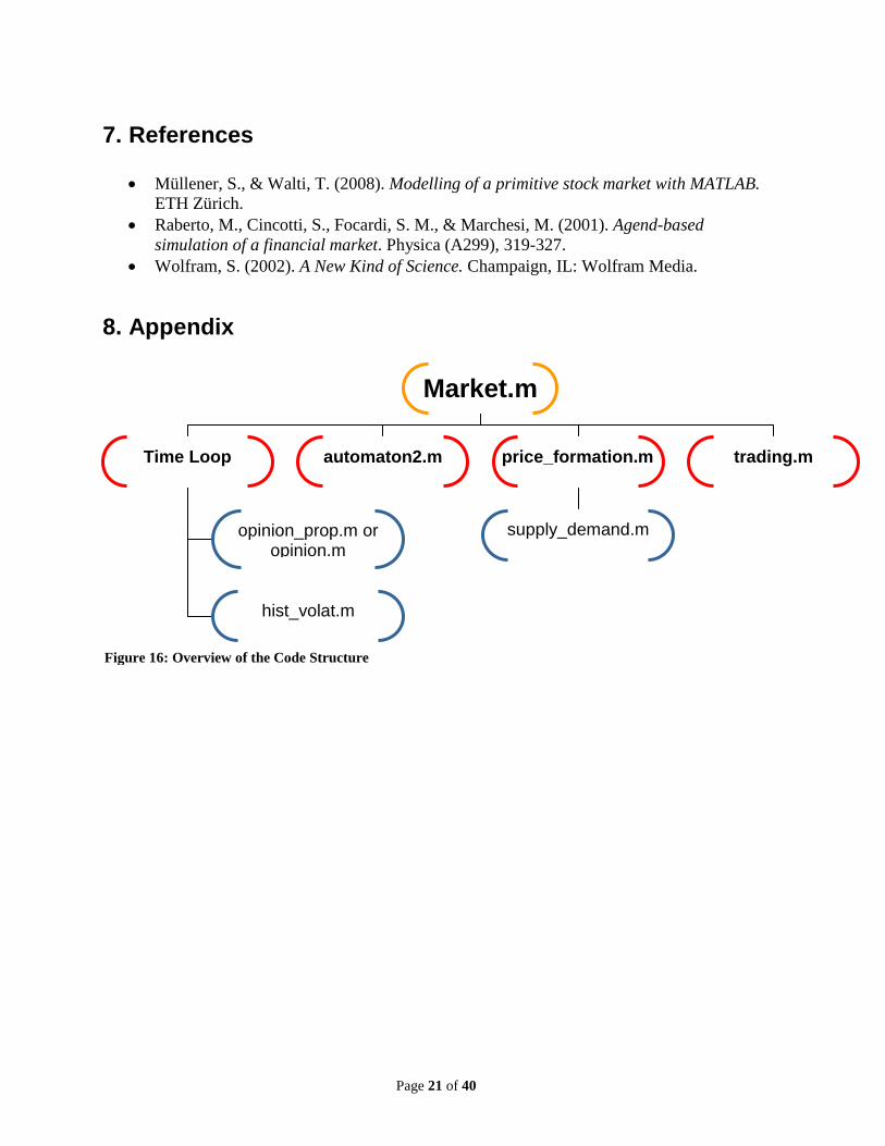
4.1. The agent-based financial market model At the heart of the financial market model is the function “market.m”, which simulates the agent-based financial markets and incorporates 7 sub-functions (cf. Figure 16, Appendix). For this function, the user can specify inputs to run either the “old” or the “new” market with any combination of the following model features activated:

• trading • historic volatility • opinion propagation (two versions) • short selling

Furthermore, the user specifies the model size (number of agents) and simulation period (time-steps), as well as whether to show summary statistic plots together with the outputs. The outputs provided by the function are the full time-series over the simulation period of:

• trade volume • daily volatility • number of agents in clusters • number of agents engaging in short selling • price process

In contrast to the old code, the market model was incorporated within a function including these outputs to ease the market analysis and comparison described in the last sub-section. While the first part of the market function is concerned with the model features activation and parameter/agent initialization, the core is the main loop over all time steps. In the old model, the feature of opinion propagation has to be run in every loop while in our new code structure, with the implementation of the cellular automaton (CA), this mechanism only needs to be run once before the main loop. Then, the cluster information is extracted piecewise in every time loop from the CA dynamics by passing this information to the function “opinion.m”. This drastically reduces the computational complexity, leading to 2-3 times faster calculations of the entire model when this feature is considered. The main loop also includes the historic volatility feature, while price formation (depending on the supply and demand function) as well as the trading function are outside of this loop. The last part of the code is devoted to the new detailed analysis of the model’s outputs with particular focus on volatility and clusters. As already mentioned, the original model described by Raberto, Cincotti, Focardi, & Marchesi, 2001 limits the selling agents to sell between 0% and 100% of their current asset holdings, the percentage being determined by a random draw from a uniform distribution. To make the model more realistic, we extended this model to allow for short selling. Instead of a uniform random draw, we determine the fraction/multiple of current asset holdings to be sold by a normal random draw with the same mean as before: 0.5. Hence, there is a positive probability that an agent is selling more than 100% of his current asset holdings, i.e. short selling. To avoid a negative percentage (i.e. sellers becoming buyers), we take the absolute value of this quantity, which then of course adds more weight on the right-hand side of the distribution. This creates the intended characteristic of over-weighting the possibility of short selling. In order to keep the model symmetric, whenever the short selling feature is activated, we need to allow for credit-financed buying, the economic analogon of short selling. This is

of 40

implemented by drawing from a normal distribution with mean 0.5 to determine the “buy cash”. This enables buyers to spend more cash than they currently have on their account, which happens with a positive probability. Again, to avoid buyers to become sellers, we take the absolute value of this amount resulting in the same left skewed distribution described above. Since a main point of analysis focuses on clusters and their induced volatility, the output of the market model was extended to include these features in a separate graph. To maintain comparability, we kept the summary plots of price, returns, probability plot and density plot.

4.2. The Cellular Automaton The appendix shows the code for the cellular automaton. In lines 10-21 the automaton parameters are set. All key parameters are explained below: Probabilistic Parameters:

• “pini” defines the probability for each agent to be in a cluster at initialization of the automaton or at re-initialization after a cluster-burst

• “pd” is a probability used to curb the de-clustering effect of neighboring cells at cluster edges

• “pn” defines the level of background noise • “pdest” defines the probability of clusters being destroyed, given a certain cluster size

is achieved Cluster density limits:

• “densl” defines the local maximum allowed cluster density per area • “densg” defines the global maximum allowed cluster density per area

Redundant parameters: • “p” could be used to curb the chances of an agent to remain in a cluster, but we set this

parameter to 1 and it therefore does not impact the model • “pr” could be used to curb the clustering effect of neighboring agents through the

below rules but we set this parameter to 1 and it therefore does not impact the model Lines 27-29 initialize the output matrix of the automaton function and initialize the automaton grid with a frame such that all agents, including all edge agents have a complete neighborhood. All agents are then randomly assigned an initial state (cluster or non-cluster, i.e. 1 or 0) according to the pini parameter. Lines 34-39 define vectors of row and column indices used in the following neighborhood definitions. For example "up" contains all those indices of rows that can contain an "up-neighbor" of any agent. In the time loop, the agent cluster simulation takes place. First, the agent grid is cut into 9 equally sized squares and local maximum cluster size conditions are given according to densl. Each local area is set back to a random initial condition if the local cluster-burst conditions are met (lines 57 – 89). Lines 93 – 104 define matrices that store the information of whether or not a neighbor is currently in a cluster for the first order Moore-neighborhood (that is for all eight cells surrounding the agent cell). Exact neighbor locations are specified by use of the letters “a” to

of 40

“h”. Thus from “aga” to “agh” the information from the upper left neighbor to the lower right neighbor are stored. “ag” contains the information about the state of each agent itself. For example aga=Cells(up, left) shifts the entire agent matrix up by one step and left by one step. As a result, aga is a matrix of the same size as the actual agent matrix that stores, for any agent, the current state of its upper left neighbor. Lines 108 – 121 define the actual automaton clustering rules. Lines 108 – 113 give conditions that will cause any agent to be a cluster member at the first step in the automaton rules. In particular, any agent will be a cluster member at this stage, if the agent already is in a cluster or any adjacent pair of its first order von Neumann-neighborhood (that is of the four cells orthogonally surrounding it) is already in a cluster. For clustering, it is sufficient that any of the below four conditions is met, irrespective of the state of other neighbors, as long as the de-clustering rules do not override this. The below graph serves as an illustration: Grey cells represent current cluster members. All four states (individually) of the first order von Neumann-neighborhood shown cause an agent to become a cluster member at this stage.

b b b b d Agent e d Agent e d Agent e d Agent e g g g g

Figure 1: Clustering conditions Furthermore an agent can become a cluster member purely by chance (at very low probability) according to the parameter pn. Lines 114-121 give conditions that can cause a current cluster member to de-cluster: if such four adjacent Moore-neighborhood agents are in a cluster, that they leave a straight line of three non-cluster-Moore-neighbors, the agent might de-cluster. For de-clustering, it is necessary that all eight Moore-neighbors are in these exact states. This is intended to identify cluster members at the outer boundaries of a cluster and potentially let them de-cluster. Already mature clusters will hence be curbed. The below graph illustrates this. Grey cells again represent current cluster members. All four states (individually) of the Moore-neighborhood shown can cause an agent to de-cluster.

a b c a b c a b c a b c d Agent e d Agent e d Agent e d Agent e f g h f g h f g h f g h

Figure 2: De-clustering conditions Finally, after the automaton has updated all agents’ states according to the above rules a global maximum condition for cluster size is given. The if-statement starting in line 125 initiates the possibility of a global cluster burst from a cluster-size defined by densg. If a global burst occurs, all agents are set back to a random initial condition according to pini. This loop runs over all time steps in the simulation.

of 40

4.3. The market analysis toolkit As it is a main goal of this paper to compare and contrast the new enhanced model to the old model implemented by Müllener & Walti, 2008, we implemented an extended market analysis toolkit for this purpose. The script “MarketsAnalysis.m” is designed to conduct a “ceteris paribus” analysis of the two models’ stability over model size (i.e. number of agents). It allows for a direct comparison of output results produced by both models over a number of diffent model sizes. Usually, these are looped in decreasing order (e.g. 400 to 80 agents in steps of 40), while all other model parameters can be specified by the user and are then kept constant. The output produced within the loop plots the volatility process of the new model against the old model’s. When all agent loops are completed, the effect of changing model size is visualized in a volatility surface for both the new and the old model. “MarketsAnalysis.m” was used extensively in section 5.4. Stability Analysis over Model Size. An equally useful toolkit to conduct a “ceteris paribus” analysis of the stability of model features is the script “Trajectories.m”. In a similar fashion to the script described above, it produces multiple runs of both the old and the new model, where the user can specify all input and all model parameters, which are then kept constant. The output produced in the loop focuses on volatility and clustering, these are plotted for every “trajectory” over time for both the new and the old model. Finally all price trajectories are plotted for both models. This script file was used for all simulations conducted in section 5.3. Stability Analysis over Model Features.

5. Simulation Results and Discussion 5.1. Empirical Data vs. Model Simulation

As a first view on our model, we would like to compare the simulation results with both empirical data from the financial crisis and the old model. For the purpose of comparison, we run our model as well as the old model over 4 years (i.e. 1000 trading days) with 200 agents, including all model features. As an example of empirical data from the financial sector, we take a time-series of log returns for JP Morgan Chase over the period from 1.1.2006 to 31.12.2009 (Figure 3.a). Figure 3.b shows a sample run from the new model while Figure 3.c shows a sample run from the old model.

of 40

Figure 3: a. Empirical data b. sample trajectory from new model c. sample trajectory from old model

of 40

The figures indicate that the new model better captures the characteristics from the empirical data than the old model. In particular, one can see that the new model has the ability to produce clusters of large log returns (in periods 600 to 800) as it has appeared during the financial crisis in fall 2008, while the old model seems to be better suited to model single spikes only. However, the old model has been able to reproduce other well-known stylized facts which we have tested in our model as well.

5.2. Analyzing stylized facts As Müllener & Walti, 2008 have shown, the old model was able to capture heavy-tailed log return distributions as well as serially correlated volatility to some degree. To ease comparison, we employ the same testing toolkit for our model. Figure 4: Summary Statistics of a Simulation run (new model) shows the price dynamics of a single run, the respective log returns, a probability plot to test normality of the time-series as well as the density of log returns.

Figure 4: Summary Statistics of a Simulation run (new model). All four graphs show similar results with respect to these features, in particular the probability plot indicates a clear deviation from the normal assumption, as it is usually observed in empirical data. To verify this, we have conducted a Jarque-Bera test at the 99.9% significance level with the null hypothesis that the sample be drawn from a normal distribution. For the sample run plotted, the null hypothesis is rejected. Furthermore, our new financial markets model produces output showing the relationship between volatility and clusters, as this is the major change over the old model.

of 40

Figure 5: Agents in Clusters vs. Volatility As we can see in Figure 5, the new model allows for serially correlated clusters which in turn have a clear impact on the volatility level. Obviously, since all the figures above only show single sample runs from the new model, further analysis on the stability of such results is required.

5.3. Stability Analysis over Model Features In the following, we extend the comparison of our new model and the old model to the stability of results over model features. We conduct ten runs of each model over 2 years (i.e. 500 trading days) with 200 agents, testing the impact of the model features “short sales” and “opinion propagation”. The first stability analysis is conducted in both models using all features.

Figure 6: Ten price paths of the new model (top) vs. old model (bottom)

of 40

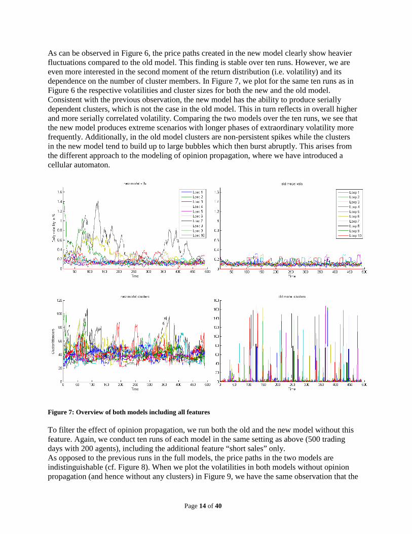
As can be observed in Figure 6, the price paths created in the new model clearly show heavier fluctuations compared to the old model. This finding is stable over ten runs. However, we are even more interested in the second moment of the return distribution (i.e. volatility) and its dependence on the number of cluster members. In Figure 7, we plot for the same ten runs as in Figure 6 the respective volatilities and cluster sizes for both the new and the old model. Consistent with the previous observation, the new model has the ability to produce serially dependent clusters, which is not the case in the old model. This in turn reflects in overall higher and more serially correlated volatility. Comparing the two models over the ten runs, we see that the new model produces extreme scenarios with longer phases of extraordinary volatility more frequently. Additionally, in the old model clusters are non-persistent spikes while the clusters in the new model tend to build up to large bubbles which then burst abruptly. This arises from the different approach to the modeling of opinion propagation, where we have introduced a cellular automaton.

Figure 7: Overview of both models including all features To filter the effect of opinion propagation, we run both the old and the new model without this feature. Again, we conduct ten runs of each model in the same setting as above (500 trading days with 200 agents), including the additional feature “short sales” only. As opposed to the previous runs in the full models, the price paths in the two models are indistinguishable (cf. Figure 8). When we plot the volatilities in both models without opinion propagation (and hence without any clusters) in Figure 9, we have the same observation that the

of 40

two models cannot be told apart. Not in a single run do we observe an extreme event with high volatility.

Figure 8: Ten price paths of the new model (top) vs. old model (bottom) without the opinion propagation feature

Figure 9: Overview of both models without the opinion propagation feature

of 40

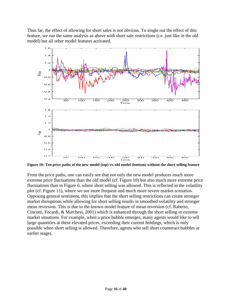
Thus far, the effect of allowing for short sales is not obvious. To single out the effect of this feature, we run the same analysis as above with short sale restrictions (i.e. just like in the old model) but all other model features activated.

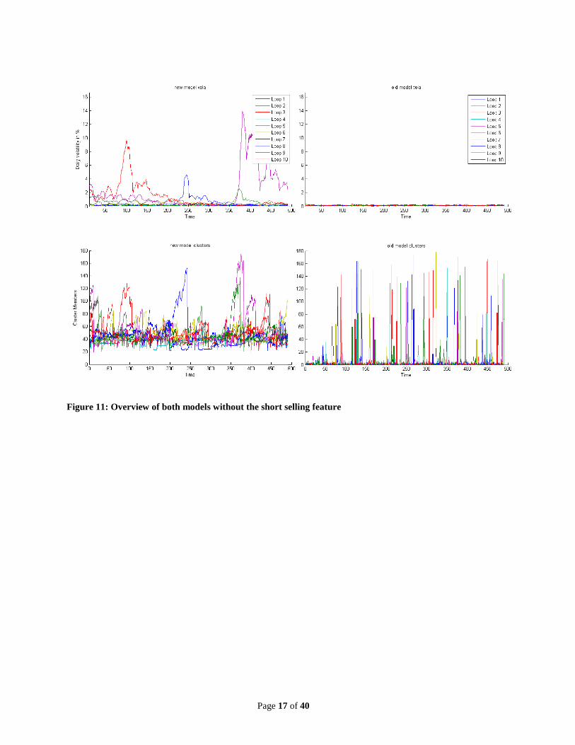
Figure 10: Ten price paths of the new model (top) vs. old model (bottom) without the short selling feature From the price paths, one can easily see that not only the new model produces much more extreme price fluctuations than the old model (cf. Figure 10) but also much more extreme price fluctuations than in Figure 6, where short selling was allowed. This is reflected in the volatility plot (cf. Figure 11), where we see more frequent and much more severe market scenarios. Opposing general sentiment, this implies that the short selling restrictions can create stronger market disruptions while allowing for short selling results in smoothed volatility and stronger mean reversion. This is due to the known model feature of mean reversion (cf. Raberto, Cincotti, Focardi, & Marchesi, 2001) which is enhanced through the short selling in extreme market situations. For example, when a price bubble emerges, many agents would like to sell large quantities at these elevated prices, exceeding their current holdings, which is only possible when short selling is allowed. Therefore, agents who sell short counteract bubbles at earlier stages.

of 40

Figure 11: Overview of both models without the short selling feature

of 40

5.4. Stability Analysis over Model Size In all above experiments, we have kept the model size (i.e. number of agents) constant at the level of 200 agents where Müllener & Walti, 2008 have tested their model. Additionally, we have analyzed the stability of the new versus the old model over the model size. We have conducted sample runs starting from a large model (400 agents), decreasing in steps of 40 agents to a very small model (80 agents). To obtain a broader view, we have increased the time period analyzed to four years (i.e. 1000 trading days). Furthermore, to maintain comparability to the old model, we have excluded short selling, which is a feature unique to the new model.

Figure 12: Size Sensitivity Analysis of both models without short selling We can observe in Figure 12, as one would expect from the previous analysis in section 5.3, that the new model has produced one extreme event within the nine loops over four years. However, there seems to be no correlation between model size and the probability of an extreme event as this has happened in the sample run with 280 agents. In the old model however, we verify the findings of Raberto, Cincotti, Focardi, & Marchesi, 2001 that volatility is sensitive to model size. This clear relationship can be seen in both Figure 14 and in Figure 15, in which we see that volatility decreases with increasing model size. In Figure 14, we see the same sample runs as a surface of volatility dynamics with respect to the number of agents, where the agent loops are ordered from many agents to few agents. In the new model, to ease visualization, we have excluded the extreme event in the sample run with 280 agents when displaying the volatility surface (cf. Figure 13). This close-up view on volatility levels in relatively calm markets allows us to identify a smaller volatility peak, which again occurs arbitrarily in the middle of the agent loops, again suggesting independence of model size. More detailed and computationally intensive analysis would be required to further strengthen this hypothesis.

of 40

Figure 13: Volatility Surface w.r.t. Agents in the new model without short selling

Figure 14: Volatility Surface w.r.t. Agents in the old model without short selling

of 40

Figure 15: Average Market Volatility w.r.t. Agents of the two models without short selling

6. Summary and Outlook To address some of the shortcomings of the Genoa market model implemented by Müllener & Walti, 2008, we have introduced short selling as an additional model feature and replaced the opinion propagation mechanism by a cellular automaton. When simulating using this new agent-based financial market model we find a better representation of real world data from the recent financial crisis. In particular, the new model better captures the autocorrelation characteristics of volatility as it can be observed in empirical data. This is due to the new modelling of agent clusters via the above mentioned cellular automaton. Furthermore, the new model also produces non-normal (i.e. heavy-tailed) distributions. The recent severe disruptions in the financial markets over the past three years justify this high frequency of extreme scenarios in our model. In light of the recent debate regarding short selling, we present another noteworthy finding within our model: deregulating the market (i.e. removing short selling restrictions) leads to a smoothing of volatility when including all model features. This is due to the fact that short selling counteracts both the emergence of bubbles and therefore also bubble-burst induced crashes. This is in stark contrast to Müllener & Walti, 2008 (p. 18) who conjecture that short selling would contribute to “undesirable” market volatility. Moreover, the above findings are stable over multiple simulation runs as well as with respect to model size. The stability of volatility overcomes the old model’s weakness of volatility dependence on model size. However, this is only a conjecture and requires further analysis which proves to be highly resource intensive. A detailed investigation of this phenomenon could be addressed in future research. Another interesting direction for further projects would be the modeling of heterogeneous agents (e.g. both reversal and momentum traders) as well as the extension of the model to more sophisticated financial products such as derivatives.

of 40

7. References

• Müllener, S., & Walti, T. (2008). Modelling of a primitive stock market with MATLAB. ETH Zürich.

• Raberto, M., Cincotti, S., Focardi, S. M., & Marchesi, M. (2001). Agend-based simulation of a financial market. Physica (A299), 319-327.

• Wolfram, S. (2002). A New Kind of Science. Champaign, IL: Wolfram Media.

8. Appendix

Market.m

Time Loop price_formation.m trading.m

opinion_prop.m or opinion.m

hist_volat.m

automaton2.m

supply_demand.m

Figure 16: Overview of the Code Structure

of 40

market.m function [tradeVolume,vola1d,Cluster,shortsale,price]= market(version,trade,histVola,opinionProp,short,T,agents,p) % This function simulatates an agent-based financial market % INPUTS are: 'new' or 'old' market model (as a string); activate (1) or % deactivate (0) the model features: trading, historic volatility, opinion % propagation and shortselling; number of timeperiods T to be simulated and % number of agents in the model; finally 0 or 1 for graphical plots % sample inputs are: market('new',1,1,1,1,500,400,1); % OUTPUTS are: trading Volume in the market, the daily volatility, the % number of agents in clusters, number of shortsales and the price proces tic %% Model Features TRADING = trade; HISTORICAL_VOLATILITY = histVola; OPINION_PROPAGATION_CLUSTERS = opinionProp; SHORTSELLING=short; PLOTS=p; if strcmp(version,'new') NEWMARKET=1; else NEWMARKET=0; end; %% Parameter Initialisation global agent; global t; global globalBuyProb; global clusterPairProbability; global clusterActivateProbability; global activatedClusterSize; global clusters; global buySigmaK; global sellSigmaK; global timeSteps; global N; global stockPrice; timeSteps = T; N = agents; PercentageDone = 0; % set global market parameters stockPrice = ones(timeSteps,1); activatedClusterSize = zeros(timeSteps,1); clusters = zeros(N,1); % maximum number of possible clusters: N/2 clusterPairProbability = 0.0001; clusterActivateProbability = 0.2; tradeVolume = zeros(timeSteps,1); vola1d=zeros(timeSteps,1); shortsale=zeros(timeSteps,1);

of 40

% set global agent parameters globalBuyProb = .5; sellMu = 1.01; sellSigmaK = 3.5; buyMu = 1.01; buySigmaK = 3.5; shortSigma = 0.2; % initializing the agents individual parameters for n = 1:N agent(n).cash = 1000; agent(n).assets = 1000; agent(n).volatSigma = 0.02; agent(n).volatTimeInt = 50; agent(n).buyProb = globalBuyProb; agent(n).isBuyer = 0; agent(n).isSeller = 0; agent(n).buyCash = 0; agent(n).buyQuant = 0; agent(n).buyUpperLimit = 0; agent(n).sellQuant = 0; agent(n).sellLowerLimit = inf; agent(n).cluster = 0; % if member of cluster: [clusternumber] | else: [0] end % running the cellular automaton if opinion propagatian is activated in the % new model if (OPINION_PROPAGATION_CLUSTERS && NEWMARKET==1) Cells=automaton2(N,timeSteps,PLOTS); end %% Main Loop for t = 1:timeSteps %% Opinion Propagation in the old model if OPINION_PROPAGATION_CLUSTERS && NEWMARKET==0 opinion_prop() end %% Opinions Propagation in the new model if OPINION_PROPAGATION_CLUSTERS && NEWMARKET==1 % passing the CA output to the opinion function, which returns a vector % of reset buy probabilites for all agents [buyProb,activatedClusterSize(t)]=opinion(Cells(:,:,t)); for n = 1:length(buyProb) agent(n).buyProb=buyProb(n); end end for n = 1:N %% Agent is Buyer or Seller during this time-step? if rand(1)<agent(n).buyProb %randomly choosing buyers

of 40

agent(n).isSeller = 0; agent(n).isBuyer = 1; % buyCash update: if short-selling is activated, then exceedance of current % cash account is allowed (credit buying); else short-selling constraint if SHORTSELLING agent(n).buyCash = abs(normrnd(0.5,shortSigma))*agent(n).cash; else agent(n).buyCash = rand(1)*agent(n).cash; end else %rest are sellers agent(n).isSeller = 1; agent(n).isBuyer = 0; % sellQuant update: if short-selling is activated, then exceedance of % current asset level is allowed; else short-selling constraint if SHORTSELLING agent(n).sellQuant = round(abs(normrnd(0.5,shortSigma))*agent(n).assets); else agent(n).sellQuant = round(rand(1)*agent(n).assets); end % counting incidenct of short-selling if agent(n).sellQuant>agent(n).assets shortsale(t)=shortsale(t)+1; end end %% Historial Volatility if HISTORICAL_VOLATILITY hist_volat(n) end %% Agent buy or sell parameters if (agent(n).isBuyer == 1) agent(n).buyUpperLimit = stockPrice(t)*(normrnd(buyMu,agent(n).volatSigma)); agent(n).buyQuant = round(agent(n).buyCash/agent(n).buyUpperLimit); else agent(n).sellLowerLimit = stockPrice(t)/abs(normrnd(sellMu,agent(n).volatSigma)); end end %% New Market Price stockPrice(t+1) = price_formation(stockPrice(t)); %% Trading if TRADING tradeVolume(t)=trading(); end if PLOTS if PercentageDone ~= round(100*(t/timeSteps)) PercentageDone = round(100*(t/timeSteps)) end end end

of 40

% Calculate 10d-averaged daily Volatility voladays=10; %number of days to average the volatility stockPriceReturnLog = log(stockPrice(2:end))-log(stockPrice(1:end-1)); %calculating log price returns % calculation of the daily volatility for i=1:(timeSteps-(voladays-1)) vola1d(i+voladays-1)=std(stockPriceReturnLog(i:(i+voladays-1)))/sqrt(voladays); end price=stockPrice(2:end); % the stock price process Cluster=activatedClusterSize; % the cluster size process %% PLOT THE DATA if PLOTS % plot options figure('Name','Financial Market Summary') hold on % Stock price process subplot(2,2,1) plot(price) title('Price Dynamics') xlabel('Time') ylabel('Price') % Log return of the Stock price subplot(2,2,2) plot(100*stockPriceReturnLog) title('Price Log Returns') xlabel('Time') ylabel('Log Returns in %') % Probplot of the log price return subplot(2,2,3) probplot(stockPriceReturnLog) % Estimate of the PDF subplot(2,2,4) ksdensity(stockPriceReturnLog) title('Density of Log-Returns') xlabel('Data') ylabel('Frequency') hold off % Plot Clusters vs. Volatility figure('Name','Agents in Clusters and Volatility') AX=plotyy(voladays:timeSteps,activatedClusterSize(voladays:timeSteps),voladays:timeSteps,100*vola1d(voladays:timeSteps)); set(get(AX(1),'Ylabel'),'String','Agents in Clusters') set(get(AX(2),'Ylabel'),'String','Volatility in %') xlabel('Time') end toc end

of 40

opinion_prop.m function [] = opinion_prop() % This function forms clusters amongst agents by resetting their buy % probabilites to obtain "sure buyers" and "sure sellers". % NOTE: This is the opinion propagation mechanism for the OLD model only global agent global N global t global globalBuyProb global clusterPairProbability global clusterActivateProbability global activatedClusterSize global clusters %% Pairing: defining which agents belong to a cluster % Reset last buyProb at first (changed for activated clusters) agent(N).buyProb = globalBuyProb; for i = 1:N-1 % Reset all buyProb to globalBuyProb (changed for activated clusters) agent(i).buyProb = globalBuyProb; for j = i+1:N % form pair with Pa if rand(1)<clusterPairProbability && ... ((agent(i).cluster~=agent(j).cluster ) || agent(i).cluster==0) % form pair: % if i agent is member of cluster: % set j agent (and all his cluster members) % to i cluster (and free j cluster) if agent(i).cluster~=0 if agent(j).cluster~=0 clusters(agent(j).cluster)=0; clusterToChange = agent(j).cluster; for k = 1:N if agent(k).cluster==clusterToChange agent(k).cluster=agent(i).cluster; end end end agent(j).cluster=agent(i).cluster; % elseif j agent is member of cluster (and i is not): % set i agent to j cluster elseif agent(j).cluster~=0 agent(i).cluster = agent(j).cluster; % else % form new cluster and reserve slot in cluster-arr else k = 1; while clusters(k)~=0; k=k+1; end %if k ~= 1; keyboard; end clusters(k)=1; agent(i).cluster = k;

of 40

agent(j).cluster = k; end end end end %% Cluster activation: activate a single cluster of agents if rand(1)<clusterActivateProbability % find nonzero clusters activeClusters = find(clusters); % random draw of a cluster (first element after randperm) randElemNum = randperm(length(activeClusters)); %activeClusters = randperm(activeClusters); % activate the cluster if ~isempty(activeClusters) if rand(1)<0.5 buyProb = 0; else buyProb = 1; end tempSum = 0; for k = 1:N if agent(k).cluster == activeClusters(randElemNum(1)); agent(k).buyProb = buyProb; agent(k).cluster = 0; % leave cluster tempSum = tempSum + 1; end end activatedClusterSize(t) = tempSum; if activatedClusterSize > 0.95*N %keyboard % Too big a cluster was activated end clusters(activeClusters(randElemNum(1)))=0; % free cluster end end end

of 40

opinion.m function [buyProb,sum]=opinion(Cells) % identifying clusters in Cellular Automaton output and randomly resetting % buy Probability of agents in that cluster % INPUT: a n-by-n matrix coming from the CA output with % n*n=N, the total number of agents in the market model % OUTPUT: a vector of length N with buy probabilites for all agents /buyProb) as % well as the number of agents in clusters (sum) % number of agents in the model N=length(Cells)^2; % indentifying the clusters in the CA % output and counting the number of clusters [Cluster,numb]=bwlabel(Cells); buyProb=ones(N,1)/2; sum=0; % extracting each cluster of agents and its sizes for i=1:numb %returning the vector of cluster members a = find(Cluster==i); size=length(a); sum=sum+size; % randomly allocating buyers/sellers if rand(1)<0.5 buy=0; else buy=1; end for k=1:size buyProb(a(k))=buy; end end end

of 40

hist_volat.m function [] = hist_volat(n) % This function resets the nth agent's historic volatility % INPUT: agent number % % OUTPUT: none % global agent global t global stockPrice global buySigmaK global sellSigmaK %calculate volatSigma if t==1 agent(n).volatSigma = 0; else if t < agent(n).volatTimeInt stockPricesRecent = stockPrice(1:t); logPriceReturn = log( stockPricesRecent(2:end)./stockPricesRecent(1:end-1) ); else stockPricesRecent = stockPrice(t-agent(n).volatTimeInt+1:t); logPriceReturn = log( stockPricesRecent(2:end)./stockPricesRecent(1:end-1) ); end if (agent(n).isBuyer == 1) agent(n).volatSigma = buySigmaK * std(logPriceReturn); else agent(n).volatSigma = sellSigmaK * std(logPriceReturn); end end

of 40

Automaton2.m function[ClusterDynamics]=automaton2(agents,periods,plot) %This function uses a stochastic cellular automaton to model cluster %building amongst all agents over the specified time horizon tic %Parameter SetUp: Lines 10 - 21: pini=0.15; p=1; pr=1; pd=0.6; pn=0.0003; pdest=0.1; N=round(sqrt(agents)); T=periods; densl=0.85; densg=0.25; PLOTS=plot; % Initialisations Lines 27 - 29: ClusterDynamics=zeros(N,N,T); Cells=zeros(N+2,N+2); Cells(2:N+1,2:N+1)=(rand(N,N)<pini); % Row/column indices set up Lines 34 - 39: up=(1:N); down=(3:N+2); center_rows=(2:N+1); left=(1:N); right=(3:N+2); center_cols=(2:N+1); if PLOTS figure('Name','Agent Cluster Dynamics') subplot(1,2,1) imagesc(Cells(center_rows,center_cols)) colormap(gray)

of 40

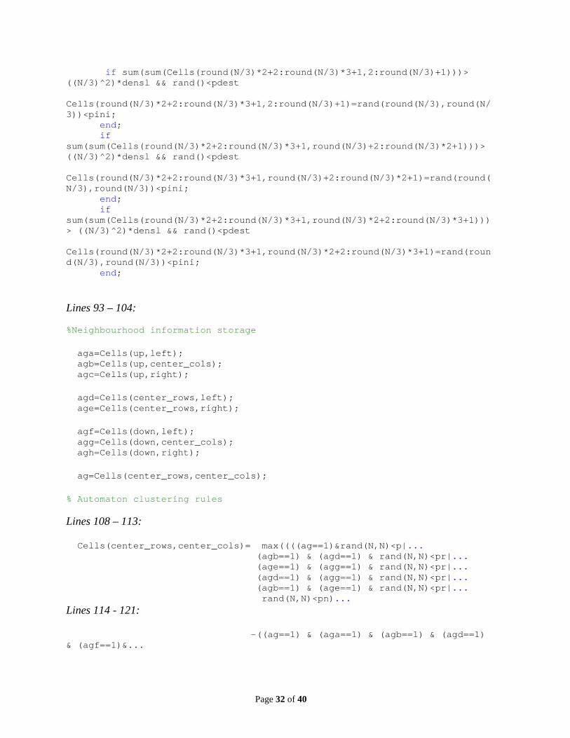
title('Initial state') drawnow; end for i=1:T Lines 57 – 89: % Local Cluster Limitations % Three upper squares: if sum(sum(Cells(2:round(N/3)+1,2:round(N/3)+1)))> ((N/3)^2)*densl && rand()<pdest Cells(2:round(N/3)+1,2:round(N/3)+1)=rand(round(N/3),round(N/3))<pini; end; if sum(sum(Cells(2:round(N/3)+1,round(N/3)+2:round(N/3)*2)+1))> ((N/3)^2)*densl && rand()<pdest Cells(2:round(N/3)+1,round(N/3)+2:round(N/3)*2+1)=rand(round(N/3),round(N/3))<pini; end; if sum(sum(Cells(2:round(N/3)+1,round(N/3)*2+2:round(N/3)*3+1)))> ((N/3)^2)*densl && rand()<pdest Cells(2:round(N/3)+1,round(N/3)*2+2:round(N/3)*3+1)=rand(round(N/3),round(N/3))<pini; end; % Three middle squares: if sum(sum(Cells(round(N/3)+2:round(N/3)*2+1,2:round(N/3)+1)))> ((N/3)^2)*densl && rand()<pdest Cells(round(N/3)+2:round(N/3)*2+1,2:round(N/3)+1)=rand(round(N/3),round(N/3))<pini; end; if sum(sum(Cells(round(N/3)+2:round(N/3)*2+1,round(N/3)+2:round(N/3)*2+1)))> ((N/3)^2)*densl && rand()<pdest Cells(round(N/3)+2:round(N/3)*2+1,round(N/3)+2:round(N/3)*2+1)=rand(round(N/3),round(N/3))<pini; end; if sum(sum(Cells(round(N/3)+2:round(N/3)*2+1,round(N/3)*2+2:round(N/3)*3+1)))> ((N/3)^2)*densl && rand()<pdest Cells(round(N/3)+2:round(N/3)*2+1,round(N/3)*2+2:round(N/3)*3+1)=rand(round(N/3),round(N/3))<pini; end; % Three lower squares:

of 40

if sum(sum(Cells(round(N/3)*2+2:round(N/3)*3+1,2:round(N/3)+1)))> ((N/3)^2)*densl && rand()<pdest Cells(round(N/3)*2+2:round(N/3)*3+1,2:round(N/3)+1)=rand(round(N/3),round(N/3))<pini; end; if sum(sum(Cells(round(N/3)*2+2:round(N/3)*3+1,round(N/3)+2:round(N/3)*2+1)))> ((N/3)^2)*densl && rand()<pdest Cells(round(N/3)*2+2:round(N/3)*3+1,round(N/3)+2:round(N/3)*2+1)=rand(round(N/3),round(N/3))<pini; end; if sum(sum(Cells(round(N/3)*2+2:round(N/3)*3+1,round(N/3)*2+2:round(N/3)*3+1)))> ((N/3)^2)*densl && rand()<pdest Cells(round(N/3)*2+2:round(N/3)*3+1,round(N/3)*2+2:round(N/3)*3+1)=rand(round(N/3),round(N/3))<pini; end; Lines 93 – 104: %Neighbourhood information storage aga=Cells(up,left); agb=Cells(up,center_cols); agc=Cells(up,right); agd=Cells(center_rows,left); age=Cells(center_rows,right); agf=Cells(down,left); agg=Cells(down,center_cols); agh=Cells(down,right); ag=Cells(center_rows,center_cols); % Automaton clustering rules Lines 108 – 113: Cells(center_rows,center_cols)= max((((ag==1)&rand(N,N)<p|... (agb==1) & (agd==1) & rand(N,N)<pr|... (age==1) & (agg==1) & rand(N,N)<pr|... (agd==1) & (agg==1) & rand(N,N)<pr|... (agb==1) & (age==1) & rand(N,N)<pr|... rand(N,N)<pn)... Lines 114 - 121: -((ag==1) & (aga==1) & (agb==1) & (agd==1) & (agf==1)&...

of 40

(agg==1) & (agc==0) & (age==0) & (agh==0) & rand(N,N)<pd)... -((ag==1) & (agb==1) & (agc==1) & (age==1) & (agh==1)&... (agg==1) & (aga==0) & (agd==0) & (agf==0) & rand(N,N)<pd)... -((ag==1) & (agd==1) & (aga==1) & (agb==1) & (agc==1)&... (age==1) & (agf==0) & (agg==0) & (agh==0) & rand(N,N)<pd)... -((ag==1) & (agd==1) & (agf==1) & (agg==1) & (agh==1)&... (age==1) & (aga==0) & (agb==0) & (agc==0) & rand(N,N)<pd)), zeros(N,N)); % Global Cluster Limitations Line 125: if (sum(sum(Cells)) > (N*N)*densg) && rand()<pdest Cells(center_rows,center_cols)=(rand(N,N)<pini); end; Cells2=Cells(center_rows,center_cols); ClusterDynamics(:,:,i)=Cells2; if PLOTS subplot(1,2,2) imagesc(Cells2) colormap(gray) title('Dynamics over time') drawnow; end end toc end

of 40

price_formation.m function [p] = price_formation(marketPriceLast) % this function balances supply and demand to determine the current market % price from the previous market prices % INPUT: the price in period t-1 % OUTPUT: the price in period t %% Price Formation pLower = 0; pUpper = 10*marketPriceLast; % check whether demand f(pLower)>g(pLower) supply AND f(pUpper)<g(pUpper) at beginning % exit with old price if not [f1,g1] = supply_demand(pLower); [f2,g2] = supply_demand(pUpper); if f1<=g1 p = 0; elseif f2>=g2 p = 10 * marketPriceLast; else pTest = (pUpper+pLower)/2; [f,g] = supply_demand(pTest); while((pUpper-pLower)>marketPriceLast/1000 && f~=g) pTest = (pUpper+pLower)/2; [f,g] = supply_demand(pTest); if f>g pLower=pTest; else pUpper=pTest; end end p = pTest; end end

of 40

supply_demand.m function [f,g] = supply_demand(p) %This function determines the supply and demand for a given market price % INPUT: the current market price p % OUTPUT: the aggregate demand and aggregate supply in the market model global agent global N %% Supply/Demand values for given price p f = 0; g = 0; for n = 1:N %% Buy orders if agent is buyer and reservation price >= marketprice if (agent(n).buyUpperLimit>=p)&&(agent(n).isBuyer) f = f + agent(n).buyQuant; %% Sell orders if agent is seller and reservation price <= marketprice elseif (agent(n).sellLowerLimit<=p)&&(agent(n).isSeller) g = g + agent(n).sellQuant; end end end

of 40

trading.m function [Volume] = trading() % This function is simulating the trading mechanism % INPUT: none required % % OUTPUT: the volume of trades conducted in this period % global agent global t global N global stockPrice % lower bound of stocks to trade [f,g] = supply_demand(stockPrice(t+1)); Volume = min(f,g); tradedSell(t) = 0; tradedBuy(t) = 0; for n = 1:N if agent(n).isSeller == 1 if stockPrice(t+1)>=agent(n).sellLowerLimit && tradedSell(t)<Volume % This seller sells numAssetsToSell = min(agent(n).sellQuant, Volume-tradedSell(t)); agent(n).assets = agent(n).assets-numAssetsToSell; tradedSell(t) = tradedSell(t) + numAssetsToSell; agent(n).cash = agent(n).cash + (numAssetsToSell * stockPrice(t+1)); end else if stockPrice(t+1)<=agent(n).buyUpperLimit && tradedBuy(t)<Volume % This buyer buys numAssetsToBuy = min(agent(n).buyQuant, Volume-tradedBuy(t)); agent(n).assets = agent(n).assets+numAssetsToBuy; tradedBuy(t) = tradedBuy(t) + numAssetsToBuy; totalBuyPrice = numAssetsToBuy * stockPrice(t+1); agent(n).cash = agent(n).cash - totalBuyPrice; end end end

of 40

MarketsAnalysis.m % To systematically compare the new model (CA opinions) with the old market and to interpret results % The analysis is conducted over different model sizes (i.e. number of agents) clear all close all clc tic % Enabling Features of the Markets trading = 1; %trading historicVola = 1; %historic vola opinionPropagation = 1; %opinion prop short = 1; %allows shortselling % simulation periods T=500; % number of agents start = 400; finish = 80; steps = -40; loops = (finish-start)/steps+1; irrel = 0; threshold = 50; % non-plotting values % initializing output variables volume=zeros(T,loops); vola=zeros(T,loops); clusters=zeros(T,loops); shortsales=zeros(T,loops); price=zeros(T,loops); volume2=zeros(T,loops); vola2=zeros(T,loops); clusters2=zeros(T,loops); shortsales2=zeros(T,loops); price2=zeros(T,loops); voladays=10; %Main Loop figure('Name','new versus old model') for d=start:steps:finish i=(d-start)/steps+1; % running both models with d number of agents [volume(:,i),vola(:,i),clusters(:,i),shortsales(:,i),price(:,i)]=market('new',trading,historicVola,opinionPropagation,short,T,d,0); [volume2(:,i),vola2(:,i),clusters2(:,i),shortsales2(:,i),price2(:,i)]=market('old',trading,historicVola,opinionPropagation,short,T,d,0); %plotting volatility outputs Amax=max(max(vola)); Bmax=max(max(vola2)); scale=max(Amax,Bmax)*100*1.2; subplot(1,2,1)

of 40

title('new model') hold on plot(vola(voladays:T,:)*100) axis([voladays,T,0,scale]) s{i} = sprintf('Agents %i', d); legend(s) xlabel('Time') ylabel('Daily volatility in %') subplot(1,2,2) title('old model') hold on plot(vola2(voladays:T,:)*100) axis([voladays,T,0,scale]) legend(s) xlabel('Time') % counting the non-plotting values if d<threshold irrel=irrel+1; end pause(0.05) end legend(s) hold off % creating a volatility surface with the new model data figure('Name','Volatility Surface: new model') surf(vola(voladays:T,1:loops-irrel)*100,'DisplayName','Volatility Surface') title('Volatility Surface w.r.t. Agents: new model') xlabel('Agent-Loop') ylabel('Time') zlabel('Daily volatility in %') % creating a volatility surface with the old model data figure('Name','Volatility Surface: old model') surf(vola2(voladays:T,1:loops-irrel)*100,'DisplayName','Volatility Surface') title('Volatility Surface w.r.t. Agents: old model') xlabel('Agent-Loop') ylabel('Time') zlabel('Daily volatility in %') % displaying the average volatility in the two markets figure('Name','Average Market Volatility') plot(start:steps:finish,nanmean(vola)*100,start:steps:finish,nanmean(vola2)*100) title('Average Market Volatility w.r.t. Agents of the two models') legend('new model','old model'); xlabel('Agents') ylabel('Daily volatility in %') toc

of 40

Trajectories.m % To systematically compare the new model (CA opinions) with the old market and to interpret results % The analysis is conducted to test the stability of the models over multiple runs clear all close all clc tic % Enabling Features of the Markets trading = 1; %trading historicVola = 1; %historic vola opinionPropagation = 1; %opinion prop short = 1; %allows shortselling T = 1000; %simulation periods agents=200; %number of agents loops=10; %specify the number of runs % initializing output variables volume=zeros(T,loops); vola=zeros(T,loops); clusters=zeros(T,loops); shortsale=zeros(T,loops); price=ones(T,loops); volume2=zeros(T,loops); vola2=zeros(T,loops); clusters2=zeros(T,loops); shortsales2=zeros(T,loops); price2=zeros(T,loops); voladays=10; %Main Loop figure('Name','new versus old model') for i=1:loops % running both models in each loop [volume(:,i),vola(:,i),clusters(:,i),shortsale(:,i),price(:,i)]=market('new',trading,historicVola,opinionPropagation,short,T,agents,0); [volume2(:,i),vola2(:,i),clusters2(:,i),shortsales2(:,i),price2(:,i)]=market('old',trading,historicVola,opinionPropagation,short,T,agents,0); %plotting volatility outputs Amax=max(max(vola)); Bmax=max(max(vola2)); scale=max(Amax,Bmax)*100*1.2; s{i} = sprintf('Loop %i', i); subplot(2,2,1) title('new model vola') hold on plot(vola(voladays:T,:)*100) axis([voladays,T,0,scale])

of 40

legend(s) xlabel('Time') ylabel('Daily volatility in %') subplot(2,2,2) title('old model vola') hold on plot(vola2(voladays:T,:)*100) axis([voladays,T,0,scale]) legend(s) xlabel('Time') ylabel('Daily volatility in %') %plotting cluster outputs subplot(2,2,3) title('new model clusters') hold on plot(clusters(voladays:T,:)) xlabel('Time') ylabel('Cluster Members') subplot(2,2,4) title('old model clusters') hold on plot(clusters2(voladays:T,:)) xlabel('Time') ylabel('Cluster Members') pause(0.05) end hold off % plotting the price paths in both models figure('Name','Price Trajectories new model') plot(price(1:T-1,:)); xlabel('Time') ylabel('Price Dynamics') legend(s) figure('Name','Price Trajectories old model') plot(price2(1:T-1,:)); xlabel('Time') ylabel('Price Dynamics') legend(s)

project report - eth z · matlab . project report . agent-based financial ... we hereby agree to...

Documents