evaporation of freely suspended single...
TRANSCRIPT

Evaporation of freely suspended single droplets: experimental, theoretical and computational
simulations
This article has been downloaded from IOPscience. Please scroll down to see the full text article.
2013 Rep. Prog. Phys. 76 034601
(http://iopscience.iop.org/0034-4885/76/3/034601)
Download details:
IP Address: 148.81.45.237
The article was downloaded on 26/02/2013 at 09:27
Please note that terms and conditions apply.
View the table of contents for this issue, or go to the journal homepage for more
Home Search Collections Journals About Contact us My IOPscience

IOP PUBLISHING REPORTS ON PROGRESS IN PHYSICS
Rep. Prog. Phys. 76 (2013) 034601 (19pp) doi:10.1088/0034-4885/76/3/034601
Evaporation of freely suspended singledroplets: experimental, theoretical andcomputational simulationsR Hołyst1, M Litniewski1, D Jakubczyk2, K Kolwas2, M Kolwas2,K Kowalski2, S Migacz2, S Palesa2 and M Zientara2
1 Institute of Physical Chemistry of the Polish Academy of Sciences Kasprzaka 44/52,01-224 Warsaw, Poland2 Institute of Physics of the Polish Academy of Sciences al. Lotnikow 32/46, 02-668 Warsaw, Poland
E-mail: [email protected] and [email protected]
Received 1 December 2011, in final form 29 November 2012Published 25 February 2013Online at stacks.iop.org/RoPP/76/034601
AbstractEvaporation is ubiquitous in nature. This process influences the climate, the formation ofclouds, transpiration in plants, the survival of arctic organisms, the efficiency of carengines, the structure of dried materials and many other phenomena. Recent experimentsdiscovered two novel mechanisms accompanying evaporation: temperature discontinuityat the liquid–vapour interface during evaporation and equilibration of pressures in thewhole system during evaporation. None of these effects has been predicted previously byexisting theories despite the fact that after 130 years of investigation the theory ofevaporation was believed to be mature. These two effects call for reanalysis of existingexperimental data and such is the goal of this review. In this article we analyse theexperimental and the computational simulation data on the droplet evaporation of severaldifferent systems: water into its own vapour, water into the air, diethylene glycol intonitrogen and argon into its own vapour. We show that the temperature discontinuity at theliquid–vapour interface discovered by Fang and Ward (1999 Phys. Rev. E 59 417–28) is arule rather than an exception. We show in computer simulations for a single-componentsystem (argon) that this discontinuity is due to the constraint of momentum/pressureequilibrium during evaporation. For high vapour pressure the temperature is continuousacross the liquid–vapour interface, while for small vapour pressures the temperature isdiscontinuous. The temperature jump at the interface is inversely proportional to thevapour density close to the interface. We have also found that all analysed data aredescribed by the following equation: da/dt = P1/(a + P2), where a is the radius of theevaporating droplet, t is time and P1 and P2 are two parameters. P1 = −λ�T/(qeffρL),where λ is the thermal conductivity coefficient in the vapour at the interface, �T is thetemperature difference between the liquid droplet and the vapour far from the interface,qeff is the enthalpy of evaporation per unit mass and ρL is the liquid density. The P2
parameter is the kinetic correction proportional to the evaporation coefficient. P2 = 0only in the absence of temperature discontinuity at the interface. We discuss variousmodels and problems in the determination of the evaporation coefficient and discussevaporation scenarios in the case of single- and multi-component systems.
(Some figures may appear in colour only in the online journal)
0034-4885/13/034601+19$88.00 1 © 2013 IOP Publishing Ltd Printed in the UK & the USA
Rep. Prog. Phys. 76 (2013) 034601 R Hołyst et al
Contents
1. Introduction 22. The evaporation model based on the Maxwell
description 32.1. Kinetic effects 5
3. Discussion of evaporation coefficient issues 63.1. The obscuring effect of impurities 7
4. Experimental apparatus and data processingprocedures 7
5. Theory versus experiment 9
5.1. Evaporation limited by diffusion of moleculesin the vapour 10
5.2. Evaporation limited by the transport of heat 105.3. Slower versus faster evaporation 105.4. Statistical rate theory 11
6. Molecular dynamics simulations 127. Summary 15Acknowledgments 17References 17
1. Introduction
Evaporation is a process ubiquitous in nature [1] andtechnology [2]. This process influences not only the climate[1, 3, 4], the formation of clouds [5], transpiration in plants
[6], the survival of arctic organisms [7], the efficiency ofcar engines [8], but also the structures of dried materials[9–11]. Solar radiation is not completely absorbed by theEarth’s atmosphere—the ocean’s surface collects most ofthe incoming solar radiation. Thus solar radiation providesenergy for water evaporation. Water evaporation has atremendous impact on global warming, because water is themain greenhouse gas in the atmosphere [1, 3]. Even thoughthere is a small triggering by CO2, which initially influences thetropospheric temperature increase, the subsequent moisteningof the atmosphere by water vapour is considered by many tobe an important feedback mechanism [12]. Fuel evaporationin combustion engines is another process whose efficiencydetermines the fuel consumption of car engines [2, 8].
Models and theories of evaporation have been developedfor over 100 years, but experimental studies have laggedbehind the theory. Our knowledge about the dynamicpathway of this phase transition is limited and largelybased on speculations rather than on solid experimentalfacts or computer simulations. Irreversible pathwaysbetween equilibrium states are not well understood. Lessis known about general rules, which govern systems farfrom equilibrium. Even in the old fields of irreversiblethermodynamics there is plenty to be discovered. On the otherhand, experiments encountered problems in the determinationof spatial and temporal profiles of thermodynamic parametersduring evaporation including the precise measurement ofvapour pressure at the micrometre/micrometre length scales.In 1999 Ward and coworkers [13] performed experiments ofwater evaporation and determined the temperature profile ofwater and its vapour during evaporation. The temperatureof the evaporating liquid (water) was close to the triple pointand consequently the vapour pressure was low. Therefore themean free path in the vapour was large (from 9 to 25 µm).Special small thermocouples were used [13] to measure thetemperature profile with spatial resolution of the order of onemean free path in the vapour, i.e. ∼10 µm. The temperatureprofile exhibited an unexpected jump at the interface withthe vapour temperature being larger by approximately 10 K
than the liquid temperature. This liquid–vapour temperaturedifference at the interface [13] was opposite in sign to the onepredicted by the kinetic theories [14–18]. The theory predictedtemperatures smaller in the vapour than in the liquid. For theexperimental conditions of Fang and Ward [13] the classicalkinetic theory predicted a temperature jump of 0.007 K [19].Thus the theoretical prediction was three orders of magnitudetoo small and, moreover, in the opposite direction. Thisresult was surprising because the theory of evaporation wasconsidered to be mature after more than 100 years of study [20].Ward and coworkers further investigated the problem [21] andconcluded that in other substances a substantial temperaturejump at the interface also occurs. Theoretical studies of theeffect followed the experimental studies [22] to explain thephenomenon, including the statistical rate theory (SRT) forevaporation [23]. Two main effects were considered as a sourceof the jump: energy flux across the vapour and the differencebetween the vapour pressure during evaporation and the actualsaturation pressure at the liquid temperature. The transport ofenergy across the vapour phase was not considered in classicaltheories as a rate limiting step of evaporation [22, 24]. Inclassical theories more emphasis was put on the mass transportfrom the interface by diffusion or kinetic-limited motion.
Another surprising result, related to pressure profilesduring evaporation, came from computer simulations ofevaporating droplets of Lennard-Jones fluids [25–27]. Thesimulations followed the solutions of the equations ofthe irreversible thermodynamics in the two phase regionduring evaporation of argon droplets [28, 29]. Irreversiblethermodynamics studies predicted [28] that pressures areequal in the vapour phase everywhere and satisfy theLaplace law for the evaporating droplet. This observationof momentum/pressure equilibrium during evaporation wasoverlooked in all previous theoretical studies. The solutionof the equations of irreversible thermodynamics was obtainedfor a system 1 µm in size, heated at the boundaries, witha 60 nm droplet evaporating in the middle of the sphericalcontainer. The study also indicated that the main processlimiting evaporation was the transport of energy across thevapour. Due to numerical problems, the study was limited tohigh vapour densities close to the critical point. The ratio ofthe liquid density to the vapour density was at most 10. Theresults were tested in computer simulations of the Lennard-Jones fluid [25] further away from the critical point with thedensity ratio as high as 100.
2

Rep. Prog. Phys. 76 (2013) 034601 R Hołyst et al
The computer simulations confirmed that duringevaporation the momentum/pressure equilibrium is satisfiedand the Laplace law obeyed in the process even for nanoscopicdroplets (here the system size was 90 nm with a 9 nmdroplet). Mechanical equilibrium was further confirmed in theevaporation of bi- and triatomic Lennard-Jones liquids [27].The most spectacular manifestation of momentum/pressureequilibrium during evaporation was found in the computersimulations of evaporation into the vacuum. In this case themomentum flux of the evaporating liquid exactly matchedthe liquid pressure setting ‘mechanical equilibrium’ in theseextreme conditions of evaporation [26, 27]. Mechanicalequilibrium means that at every point of the system the netforce is zero. At equilibrium this condition means equalityof pressure at every part of the system. In non-equilibriumprocesses a net momentum flux should be matched by thepressure, e.g. for evaporation into the vacuum the momentumflux from the flat interface is equal to the pressure inside theevaporating liquid. Computer simulations [25] also showedthat for low vapour pressure the temperature at the interfacejumps as in the experiments of Fang and Ward [13]. Thetemperature jump was as high as 30 K, but decreased tozero for higher vapour pressures in accordance with thesolutions of the equations of irreversible thermodynamicsclose to the critical point [28]. During the last decadeprevious classical theories of evaporation based on thedetailed study of mass transport have been questioned onthe basis of these new results: the temperature jump atthe interface and momentum/pressure equilibrium duringevaporation. Although we still wait for precise measurementswhich would confirm momentum/pressure equilibrium duringevaporation, already Ward and Stanga [30] have noticedthat during evaporation the vapour pressure was close tothe saturation pressure at the liquid temperature—indicatingindirectly the momentum/pressure equilibrium in the system.
None of these effects have been fully incorporated intothe models of evaporation so far and therefore our currentunderstanding of evaporation needs deep revisions. In thispaper we perform a combined analysis of experimental andcomputational simulation data to address the aforementionedissues. The data concern: evaporation of liquids (water andargon) into its own vapour and evaporation of water andglycol into air or nitrogen atmosphere. We concentrate ourattention on the description of a particularly simple systemfor analysis: a single freely suspended droplet. We present aphenomenological equation describing the radius of the dropletas a function of time and analyse this equation. We showthat the phenomenological equation is valid in all studiedcases. The continuous description based on the irreversiblethermodynamics is presented and two major approximatemodels are given. One, which follows the original work ofMaxwell is concentrated on the mass diffusion in vapour as therate limiting step for evaporation. The second model is basedon the transport of heat across the vapour. We discuss howboth models fit the data. Additionally we show that in mostcases there are kinetic corrections to the existing data. Weshow in computer simulations that kinetic corrections appearwhen there is a temperature jump at the interface. In particular
we show that, in order to fully explain evaporation, a detailedanalysis of the temperature, density and pressure profilesduring evaporation is needed. The analysis of the mass fluxonly is not sufficient to discern between different theories. Weleave the problem of the momentum/pressure equilibrium as aconstraint in evaporation theories open, although we explainqualitatively how momentum/pressure equilibrium affects thetemperature jump at the interface.
The paper is organized as follows: In section 4 wediscuss the details of the experiments on evaporation ofdroplets trapped in electric fields. In section 2 we discuss thehydrodynamic models for evaporation, the kinetic models andcorrections to the continuous description. Section 3 is devotedto the discussion of evaporation coefficients and the influenceof impurities in a droplet upon evaporation. In section 5we fit two different models to the experimental data. Onemodel assumes that evaporation is limited by the diffusive masstransfer from the interface while the second model assumes thatthe rate limiting factor is heat transfer through the vapour to thesurface of the evaporating droplet. We also discuss SRT theoryapplied to the evaporation of water into its own vapour and intothe nearly saturated water/nitrogen vapour. Section 6 presentsa comparison between the theory discussed in the previoussection and the computational simulations of evaporatingdroplets of argon at the nanoscale. The detailed analysisof finite size effects shows how to re-scale the simulationparameters to compare the model and the experiments at themicroscale to the nanoscale simulations correctly. Section 7contains the conclusions and discussion.
2. The evaporation model based on the Maxwelldescription
The problem of the stationary evaporation of a free, spherical,motionless droplet of a pure liquid in an infinite, inert mediumwas first addressed by Maxwell [31]. His description, based onmass and heat conservation equations, is still widely utilizedand considered generally adequate. A general equation of massconservation for a spherically symmetric system may take thefollowing form [32] (compare e.g. [33]):
∂
∂t
(ρr2Yi
) = ∂
∂r
(ρr2D
∂Yi
∂r
)− ∂
∂r
(ρur2Yi
), (1)
where r is the distance from the droplet centre, ρ is thetotal density of the gaseous environment, Yi is the massfraction of component i (for a two-component system: Yvap +Yair = 1, ∂Yvap/∂r = −∂Yair/∂r; one component: Yvap ≡ 1,∂Yvap/∂r ≡ 0), D is the gas-phase (mutual) diffusioncoefficient and u is the flow (radial) velocity. In the case ofan evaporating droplet u is relative to the regressing surface.The significance of various processes that (1) encompassesvaries substantially against the system’s composition andthermodynamic conditions. We shall try to address this issue.
While the analysis of transient processes duringcombustion may require consideration of the time derivative,(quasi) stationary evaporation enables its omission. Theso-called ‘moving boundary’ effect [34] is automatically lostwhen the time derivative is dropped. For stationary but fast
3

Rep. Prog. Phys. 76 (2013) 034601 R Hołyst et al
evaporation, it should and may be accounted for by othermeans.
The mass balance at the interface requires that the steadystate vapour mass flux described with (1) equals to theevaporation rate of the droplet a2aρL, where ρL is the densityof liquid and a ≡ da/dt . The non-evaporating component isobviously not transported across the interface (the solubilityof gases in liquids is neglected here). In compact form theseconditions can be expressed as:
ρr2D∂Yi
∂r− ρur2Yi = −a2aρLδi vap, (2)
where δi vap is the Kronecker delta. It is worth noting thatthe equation of continuity for the whole system takes then asimple form:
ρur2 = a2aρL. (3)
For a two-component system, (2) for a non-evaporatingcomponent can easily be identified as the definition of Stefanflow. This flow plays an important role only for a limited rangeof thermodynamic conditions: partial vapour pressure must beat least comparable to the partial pressure of the remaining gas.For a water droplet under atmospheric conditions Stefan flowconstitutes a correction to the diffusive flow of only ∼1%. Forslowly evaporating DEG it is even smaller. Then u can be setto zero. The solution of (2) under such an approximation willbe discussed later on.
Under the assumption of stationary evaporation, ideal gas(density related to temperature via an equation of state) andconstant ρD, (1) can be easily integrated. It is convenientto write down the resulting equation in a form describing theevolution of the droplet radius (compare [35]):
a = − ρD
ρLaln
[(1 − MT∞
MairTL
pa(TL)
p
) / (1 − M
Mair
p∞p
)],
(4)
where a stands for the droplet radius, T∞ and TL aretemperatures far from the droplet and at the droplet surfacein the liquid phase, respectively, p, pa and p∞ are thetotal pressure of the gaseous environment, the partial vapourpressure at the droplet, surface and the partial vapour pressurefar from the droplet, respectively, M is the molecular massof the liquid/vapour and Mair is the effective molecular massof the ambient gas. It has been pointed out [36] that a strictlyapplied boundary condition would require TL on the gas side ofthe interface (see (10)). However, a temperature discontinuityis encountered there [13, 36], and thus, such an attitude mayintroduce significant errors. In general ρD depends on thetemperature profile T (r) and if necessary should be integratedaccordingly. For large droplets down to several micrometres,pa � psat, the equilibrium (saturation) vapour pressure at agiven temperature. However, if the droplet is relatively smallthe effects of the surface tension must also be accounted for.Then, the equilibrium vapour pressure above the interface ofradius a is expressed by the Kelvin equation (see e.g. [37]):
pa(TL) = psat(TL) exp
(M
RTLρL
2γ
a
), (5)
where γ is the surface tension of the liquid and R is theuniversal gas constant. The possible effects of the dropletcharge are negligible for micrometre-sized droplets and theeffects of impurities present in real liquids will be discussedlater on.
In the case of MT∞pa(TL) � MairTLp (negligible Stefanflow in a two-component system), (4) reduces to the Maxwellequation:
a = MD
aRρL
[p∞T∞
− pa(TL)
TL
]. (6)
For low-volatility liquids under standard conditions,several micrometre-sized droplets (surface tension energy isnegligible) and an infinite gaseous medium initially void ofvapour, the evaporation can be described with an ultimatelysimple diffusive mass transport equation [38, 39],
a = − D
ρLa
Mpsat(TL)
RTL. (7)
For a one-component system (e.g. a droplet of argon,modelled by a Lennard-Jones liquid see e.g. [40, 41],evaporating into its own vapour), (2) degenerates into (3).As a consequence u cannot be neglected though it doesnot fall within the definition of Stefan flow. Moreover, itbecomes obvious that the only possible gradient of ρ is causedby the gradient of T . Then, one-component evaporationshould be described with the equation of transport of heat andequations (4), (6) and (7) are out of place, since the mutualdiffusion cannot be simply replaced by self-diffusion.
As the evaporation taking place at the droplet’s surfaceis associated with the change of enthalpy (latent heat) theequation of the transport of mass must be, in general,accompanied by the equation of the transport of heat. Theappropriate fluid dynamics equation for energy transport in agaseous medium in a reasonably general form is [32]:
∂
∂t
(ρr2h
) = ∂
∂r
(ρr2D
∑i
hi
∂Yi
∂r
)+
∂
∂r
(λr2 ∂T
∂r
)
− ∂
∂r
(ρur2h
)+ r2 ∂p
∂t, (8)
where λ is the thermal conductivity of the gaseous medium,h, hvap and hair are enthalpies of compound gaseous medium,vapour and air, respectively; h = cP (T −T∞) where cP , beingthe specific heat capacity under constant pressure, was assumedconstant within the range of temperatures concerned.
Again, for quasi-stationary processes the time derivativesmay be dropped and the steady state transport of heat for eithera one- or two-component system can be described with thefollowing concise equation:
∂
∂r
[ρr2D
(hvap − hair
) ∂Yvap
∂r
]+
∂
∂r
(λr2 ∂T
∂r
)
− ∂
∂r
(ρur2h
) = 0. (9)
The heat transported in a gaseous medium, described withthe above equation, is balanced at the interface by the heat
4

Rep. Prog. Phys. 76 (2013) 034601 R Hołyst et al
transported from the liquid phase and the heat needed forvaporizing liquid at the surface:
λa2 ∂T
∂r
∣∣∣∣r→a(+)
= λLa2 ∂T
∂r
∣∣∣∣r→a(−)
+ a2aρLqeff , (10)
where λL is the thermal conductivity of the liquid mediumand qeff is the effective enthalpy of vaporization (per unitmass). The ‘effective value’ approach is adopted sincethe enthalpy of vaporization is defined and measured forequilibrium conditions, while droplet evaporation may be quitefar from equilibrium. It is usually assumed, and we follow thisscheme here, that the transport of heat in the liquid phase isnegligible and TL is uniform in the liquid, though in generalthere may also be a considerable temperature gradient in thedroplet.
Combining equations (9) and (10) under the assumptionof instantaneous evaporation (no heat consumption from theliquid phase) and the constant cP leads to a more generalexpression than (4) (compare e.g. [40, 41]):
a = − λ
aρLcP
ln
[1 +
cP (T∞ − TL)
qeff
]. (11)
It is worth noticing that in many cases the transfer of heatby conductivity and by diffusion is comparable. The relativeimportance of these two modes is characterized by the Lewisnumber Le = (λ/cP )/(ρD). In the case of argon dropletsevaporating into their own vapour Le � 1 with good accuracy(compare LJ simulations below; again, D is self-diffusion).For water droplets in air under standard conditions Le � 1.16.For droplets of DEG under similar conditions Le � 1. Le = 1is a readily made approximation in order to obtain formulaeof the (11) type. However, for both one- and two-componentsystems (11) can be derived without such an approximationand so is valid for any Le as far as cP is constant.
Again, under the assumption of cP (T∞ −TL) � qeff , (11)takes the form:
a = − λ
aqeffρL[T∞ − TL(t)] (12)
or
a = − ρDcP
aqeffρL[T∞ − TL(t)]
for Le = 1. It is worth noting that in the case of slow, quasi-isothermal evaporation (T∞ − TL(t) < 0.1 K), the coupling ofequations (4) and (11) (as well as for their simplified forms)via TL can be neglected, and they can be used independently.We can also use the enthalpy of vaporization measured atequilibrium qeff = q.
2.1. Kinetic effects
The equations of fluid dynamics do not hold where thegradients of described quantities are high [33]. In particular,the fluid dynamics description of droplet evaporation assumescontinuity of temperature across the interface. Close tothe critical point, it seems adequate (as was shown for
LJ e.g. in [25]) but generally is not the case [13, 36]. Similarly,a high gradient of vapour density close to the surface must beconsidered [42].
The evaporation in the region below the mean free path ofthe gas molecule from the surface is treated as kinetic-limited[43] and thus governed by the Hertz–Knudsen–Langmuir(HKL) equation. For a droplet in vacuum it takes the followingform (compare [44]):
a = −αC
ρL
psat(TL)√2πkTL
√m, (13)
where m is the mass of a molecule, k is the Boltzmann constantand αC is the evaporation coefficient. This coefficient, definedas the probability of the crossing of the interface by a moleculeimpinging on it, was introduced by Knudsen [45] to reconcilethe experimental findings with the predictions of the theory.The experimentally observed evaporation rate in the kineticregime is never greater than theoretically allowed by the kinetictheory of gases. Although conceptually seemingly simple, thiscoefficient turned out to be quite difficult to measure. There isa barrier at the gas–liquid interface, although its nature has notbeen thoroughly understood yet (see e.g. [46–49]). The issue ofevaporation into vacuum, also essential for understanding thekinetics at the gas–liquid interface, has not been satisfactorilyresolved yet (see e.g. [26, 50–53]), however it seems that theapplication of the HKL equation in its standard form may notbe adequate in that case. An especially unexpected result ispresented in [26]. The flux of evaporation of an LJ liquid intovacuum, obtained from MD calculations, was reproduced withthe HKL equation where stagnation temperature was used forTL. Here αC = 2. Such value of this factor indicates thatit cannot be interpreted straightforwardly as the evaporationcoefficient, which is defined in terms of a probability smallerthan or equal to 1 [45].
It is a standard practice [35, 38] to write a single equationaccounting both for diffusive and kinetic-limited transport. It isusually done by matching equations (6) and (13) at the distancefrom the droplet �C where the diffusive and kinetic-limitedfluxes balance. �C is comparable with the mean free path ofparticles of the surrounding gaseous medium la , although itsexact value is rather arbitrary (compare [38]), which obscuresthe physical sense of the resulting equation (e.g [38, 54]). Itmust be also kept in mind that repeating this procedure forequations (4) and (11) (accounting for the Stefan flow) wouldlead to slightly different formulae.
In our works we have followed [35, 38] and used (6), withD substituted by an effective diffusion coefficient taking intoaccount the kinetic effects
Dk(a, TL) = D
a/(a + �C) + D√
2πM/(RTL)/(aαC). (14)
It should be highlighted that in order to arrive at (14) a furtherapproximation of TL = T (a + �C) is made. It manifests as anoverestimation of αC for higher T∞ − TL (>0.3 K for water).Trying to avoid this approximation excessively complicatescalculations. However, it is possible to partially correct thevalue of αC afterwards, using the formula developed in [43].
5
Rep. Prog. Phys. 76 (2013) 034601 R Hołyst et al
Similarly, the effective thermal conductivity (with kineticeffects included) of ambient gas (moist nitrogen/air forexperiments with water in [43]) may be expressed as follows(and used in (12) instead of λ):
λk(a, TL) = λ
a/(a + �T) + λ√
2πMair/(RTL)/(aαTρcP ),
(15)
where �T and αT (the thermal accommodation coefficient)play roles analogous to �C and αC, respectively.
Two characteristic length scales can be identified in eachof the above formulae: �C and 4D/(αCv) in (14) and�T and 4λ/(αTρcP vair) in (15), where v and vair are theaverage thermal velocity of vapour and ambient gas molecules,respectively. However, it is worth noticing that
�C
4D/(αCv)� 3αCD∗
4Dand
�T
4λ/(αTρcP vair)� 3αT
4Le,
(16)
where D∗ is the coefficient of self-diffusion of vapourand the Lewis number is associated with self-diffusion inambient gas. Thus, the two length scales are linked andfurthermore �C and �T are usually (significantly) smaller. Asa consequence, a single, longer length scale aC can be usedand the dimensionless droplet radius κ can be introduced asfollows:
κ = a
aC= a
4D/(αCv)or κ = a
aC= a
4λ/(αTρcP vair),
(17)
respectively.For �C = �T � 0 (see (19) and (21) in section 5)
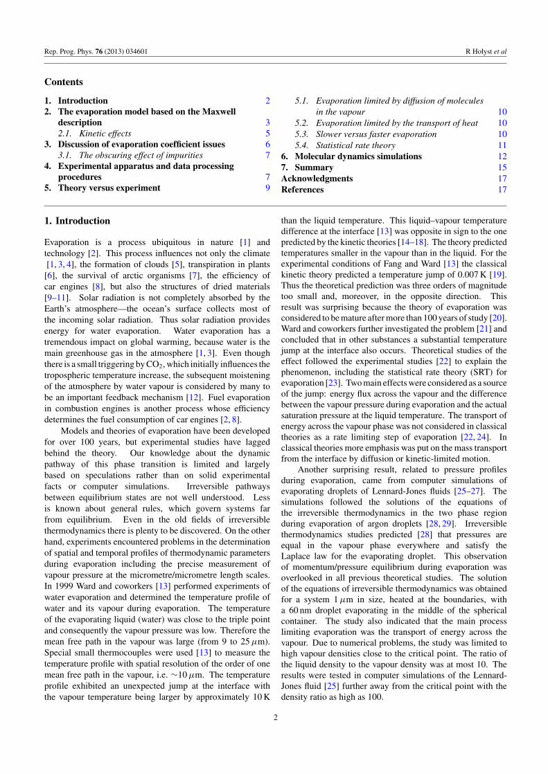
Dk(a)/D = λk(a)/λ. The magnitude of Dk and λk normalizedto D and λ for �C = �T = 0 is presented in figure 1 versusboth a and κ . It can be seen that for a dimensionless droplet ofradius 1 � κ � 5 (water droplet shrinking from ∼6 to ∼1 µm)under standard temperature and pressure (STP) conditions,the influence of kinetic effects upon the evaporation is clearlyrecognizable but not dominating.
3. Discussion of evaporation coefficient issues
Many attempts have been made over nearly a century todetermine the values of αC and αT experimentally. Most of theexperiments considered water and a variety of experimentalmethods were used. Both condensation on and evaporationfrom the surface of bulk liquid, liquid films, jets and dropletswere investigated in various environments (vacuum, standardair, passive or reactive atmospheres) under various pressuresand for various water vapour saturations. Small droplets, suchas encountered in clouds, have been favoured since kineticeffects manifest strongly for them. Suspended droplets, trainsof droplets, clouds of droplets and single trapped droplets werestudied. The results obtained by different authors spannedfrom ∼0.001 to 1 for αC and from ∼0.5 to 1 for αT (see e.g.[34, 55–62] and [38, 63–66] for reviews). There seems to bea better agreement about the value of αT. The measurementsfor other vapour–liquid systems are fewer and similarly non-conclusive. Adsorption of heterogeneous vapours on liquid
Figure 1. Effective diffusion and thermal conductivity coefficientsDk and λk normalized to D and λ, respectively, presented versusdroplet radius, both in dimensional form a and dimensionless formκ = a/aC, where the characteristic length scale aC = 1.18 µm (seedefinition (17) and compare with section 5). It should be pointed outthat for a � �C, �T Dk/D = λk/λ → κ . The calculation wasperformed for the conditions when Dk(a)/D = λk(a)/λ,corresponding to data presented in figure 6: water droplets innitrogen atmosphere, 20 ◦C, 998 hPa, αC = 0.14, αT = 0.15.
water seems to attract more attention (see [67–72] and [73]for reviews) than single-component evaporation/condensation(see [35] and references therein, and [49, 74–76]). Theresults seem to suggest that a low evaporation coefficientcorresponding to a high interfacial barrier is not unique forwater [46, 72].
Experiments with evaporation of polar liquids into vacuum(see e.g. [48] for unsteady state evaporation or [77] for jetstream tensimeter experiments and references in [65, 78]) yieldhigher values of αC than (quasi) equilibrium experiments[43, 66, 79]. On the other hand, much lower values of αC at300 K can be found in [76] and the works cited therein. Inthose studies, a so-called dropwise condensation method wasused (compare [61] for water). This method yields αC � 0.4at atmospheric pressure and αC → 0.2 for p → 0.
The measurement of temperature dependence of αC or αT
was rarely attempted and the results were inconclusive. Recentstudies for water by Li et al [55] and by Winkler et al [54] (see[66] for comparison of these studies) can serve as an example.The authors of the first study (Boston College/AerodyneResearch Inc. group) found that αC decreases with temperaturewithin the temperature range between 257 and 280 K. Theauthors of the second study (University of Vienna/Universityof Helsinki group) claim that αC and αT exhibit no temperaturedependence between 250 and 290 K. Our results for waterversus temperature [43] are in excellent agreement with thoseobtained with a fundamentally different method of the BC/ARIgroup. On the other hand, our modelling and the modellingof the UV/UH group seems to differ only by second ordereffects, while the results differ significantly. What, in ouropinion, makes a fundamental difference can be seen in thedata from [54]. They exhibit a strictly linear a2(t) dependence(the so-called D2-law, see e.g. formula (32)) which signifiesthat, quite unexpectedly, the kinetic effects do not manifest
6
Rep. Prog. Phys. 76 (2013) 034601 R Hołyst et al
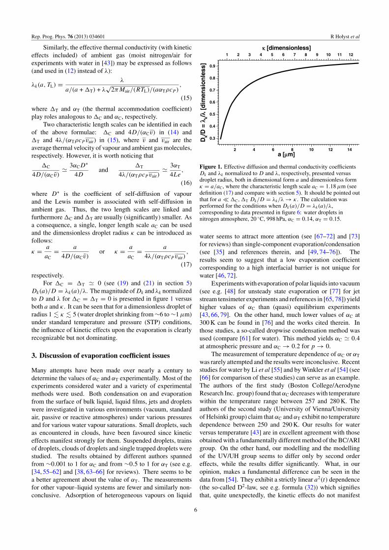
Figure 2. Estimation of the effect of impurities (ns constant isproportional to the initial mass fraction of impurities) upon dropletradius evolution for water droplets evaporating into dry nitrogenunder STP conditions. Dimensionless coordinates κ = a/aC anddκ/dτ = atC/aC, where aC = 1.14 µm and tC = 2.2 ms. Solidline—no impurities; dashed line—a small amount of impurities(ns � 5 × 10⁻⁵); dotted line—a considerable amount of impurities(ns � 1 × 10⁻³).
strongly. This probably led to an overestimation of αC. Allthese experiments show that finding a reliable value of αC is adifficult task.
3.1. The obscuring effect of impurities
Although in this work we essentially deal with pure liquids, realliquids used in experiments always contain some impurities.Real liquids may be (and usually are) simultaneouslycontaminated with substances of higher and lower volatility,as well as with non-volatile substances and insoluble particles.Although, in our experiments, we took great care to avoidimpurities and their effects, the mode of their influence uponthe observed droplet evolutions must be kept in mind. Thepresence of low-volatility (or non-volatile) impurities can beeasily observed in both figures (4) and (5) as well as infigure 6. In figure 4 it manifests as a ‘kink’ at the end of theevolution, which, after differentiation appears as a dramatic fallin figures (5) and (6). We estimated the effect of impurities forwater droplets evaporating into dry nitrogen under conditionscorresponding to the data presented in figure 6. The simplestmodel of the influence of an ideally soluble, non-surface-active, non-volatile impurity was used: the Kelvin (5) wassubstituted with the Kohler equation (compare [37, 38]):
pa(TL) = psat(TL) exp
(M
RTLρL
2γ
a− ns
(a/a0)3 − ns
), (18)
where a0 is the initial droplet radius and ns is approximatelyequal to the initial mass fraction of impurities. We used theset of equations (6), (12), (14) and (15) together with (18) formodelling. The dependence of the quantities and parametersupon temperature was also taken into account. Due to theextreme simplicity of the model the visualization presented infigure 2 is qualitative.
For higher impurity concentration, their influence issignificant and highly non-linear. Although the ‘kink’ (the
lowest trace in figure 2) can be easily isolated and avoided, theevolution is visibly slower even in the diffusion regime. Thisadditional slant and shift is noticeable even for a seeminglysmall concentration of impurities. If not accounted for, itwill mask the values of both the diffusion and the evaporationcoefficients: the diffusion coefficient would seem lower andthe evaporation coefficient higher (see [80] for details).
4. Experimental apparatus and data processingprocedures
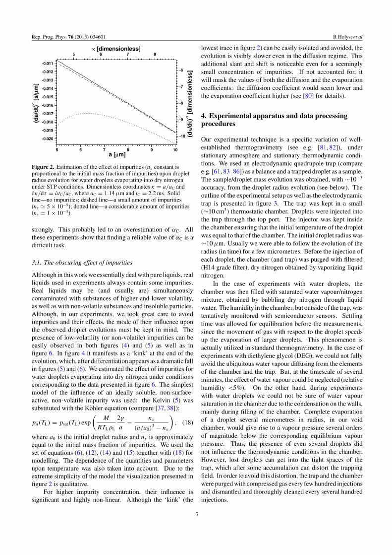
Our experimental technique is a specific variation of well-established thermogravimetry (see e.g. [81, 82]), understationary atmosphere and stationary thermodynamic condi-tions. We used an electrodynamic quadrupole trap (comparee.g. [61, 83–86]) as a balance and a trapped droplet as a sample.The sample/droplet mass evolution was obtained, with ∼10−3
accuracy, from the droplet radius evolution (see below). Theoutline of the experimental setup as well as the electrodynamictrap is presented in figure 3. The trap was kept in a small(∼10 cm3) thermostatic chamber. Droplets were injected intothe trap through the top port. The injector was kept insidethe chamber ensuring that the initial temperature of the dropletwas equal to that of the chamber. The initial droplet radius was∼10 µm. Usually we were able to follow the evolution of theradius (in time) for a few micrometres. Before the injection ofeach droplet, the chamber (and trap) was purged with filtered(H14 grade filter), dry nitrogen obtained by vaporizing liquidnitrogen.
In the case of experiments with water droplets, thechamber was then filled with saturated water vapour/nitrogenmixture, obtained by bubbling dry nitrogen through liquidwater. The humidity in the chamber, but outside of the trap, wastentatively monitored with semiconductor sensors. Settlingtime was allowed for equilibration before the measurements,since the movement of gas with respect to the droplet speedsup the evaporation of larger droplets. This phenomenon isactually utilized in standard thermogravimetry. In the case ofexperiments with diethylene glycol (DEG), we could not fullyavoid the ubiquitous water vapour diffusing from the elementsof the chamber and the trap. But, at the timescale of severalminutes, the effect of water vapour could be neglected (relativehumidity <5%). On the other hand, during experimentswith water droplets we could not be sure of water vapoursaturation in the chamber due to the condensation on the walls,mainly during filling of the chamber. Complete evaporationof a droplet several micrometres in radius, in our voidchamber, would give rise to a vapour pressure several ordersof magnitude below the corresponding equilibrium vapourpressure. Thus, the presence of even several droplets didnot influence the thermodynamic conditions in the chamber.However, lost droplets can get into the tight spaces of thetrap, which after some accumulation can distort the trappingfield. In order to avoid this distortion, the trap and the chamberwere purged with compressed gas every few hundred injectionsand dismantled and thoroughly cleaned every several hundredinjections.
7
Rep. Prog. Phys. 76 (2013) 034601 R Hołyst et al
Figure 3. Schematic view of the experimental setup (top view: droplet injector omitted). Inset: electrodynamic trap drawing (wire-framepartially rendered).
In our experiments with DEG we used diethylene glycol99.99% (BioUltra, GC, Fluka) (purity for the lot stated inGC area % by the manufacturer). For the experiments withwater, we used ultra-pure water produced in the lab (Milli-QPlus, Millipore, resistivity ∼18 M� cm, total dissolved solids<20 ppb, total organic carbon (TOC) �10 ppb, no suspendedparticles larger than 0.22 µm, microorganisms �1 colonyforming unit per ml, silicates <0.1 ppb and heavy metals�1 ppb). All liquids were transferred into the droplet injectorwith due care and without delay. The experiment wasconducted within one hour of the transfer. The effects (ionicdissolving, chemical reactions) caused e.g. by atmosphericCO2 were avoided by substituting air with nitrogen in theclimatic chamber.
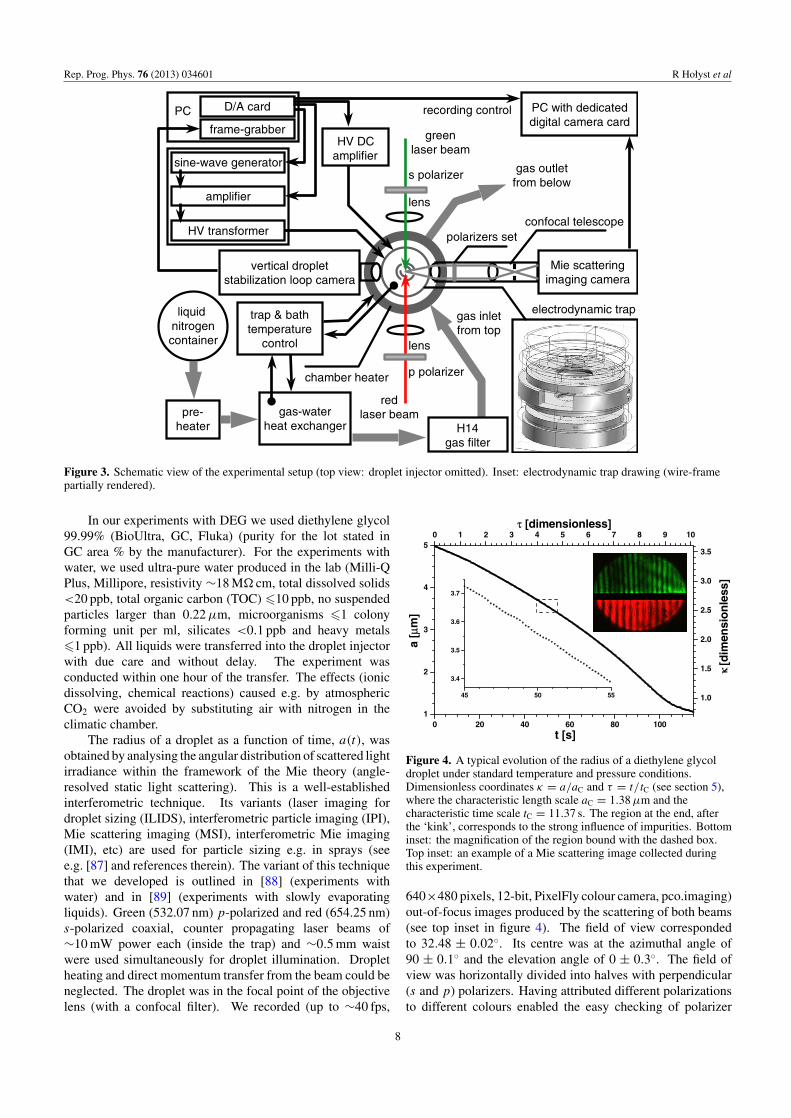
The radius of a droplet as a function of time, a(t), wasobtained by analysing the angular distribution of scattered lightirradiance within the framework of the Mie theory (angle-resolved static light scattering). This is a well-establishedinterferometric technique. Its variants (laser imaging fordroplet sizing (ILIDS), interferometric particle imaging (IPI),Mie scattering imaging (MSI), interferometric Mie imaging(IMI), etc) are used for particle sizing e.g. in sprays (seee.g. [87] and references therein). The variant of this techniquethat we developed is outlined in [88] (experiments withwater) and in [89] (experiments with slowly evaporatingliquids). Green (532.07 nm) p-polarized and red (654.25 nm)s-polarized coaxial, counter propagating laser beams of∼10 mW power each (inside the trap) and ∼0.5 mm waistwere used simultaneously for droplet illumination. Dropletheating and direct momentum transfer from the beam could beneglected. The droplet was in the focal point of the objectivelens (with a confocal filter). We recorded (up to ∼40 fps,
0 20 40 60 80 1001
2
3
4
5
a [µ
µ m]
t [s]
45 50 55
3.4
3.5
3.6
3.7
0 1 2 3 4 5 6 7 8 9 10
1.0
1.5
2.0
2.5
3.0
3.5
τ τ [dimensionless]
[dim
ensi
on
less
]κ
Figure 4. A typical evolution of the radius of a diethylene glycoldroplet under standard temperature and pressure conditions.Dimensionless coordinates κ = a/aC and τ = t/tC (see section 5),where the characteristic length scale aC = 1.38 µm and thecharacteristic time scale tC = 11.37 s. The region at the end, afterthe ‘kink’, corresponds to the strong influence of impurities. Bottominset: the magnification of the region bound with the dashed box.Top inset: an example of a Mie scattering image collected duringthis experiment.
640×480 pixels, 12-bit, PixelFly colour camera, pco.imaging)out-of-focus images produced by the scattering of both beams(see top inset in figure 4). The field of view correspondedto 32.48 ± 0.02◦. Its centre was at the azimuthal angle of90 ± 0.1◦ and the elevation angle of 0 ± 0.3◦. The field ofview was horizontally divided into halves with perpendicular(s and p) polarizers. Having attributed different polarizationsto different colours enabled the easy checking of polarizer
8

Rep. Prog. Phys. 76 (2013) 034601 R Hołyst et al
leaks (proper setup) and monitoring of depolarization. Inthe case of homogeneous droplets, light depolarization wasalso used to indicate contamination with solid particles. Thesequence of images was analysed off-line with our software(written in MATLAB). Each image was integrated with aproper distribution function over the elevation angle to ensurea better signal-to-noise ratio. The analysis was based oncomparing the azimuthal distribution of irradiance observedin each image to the library of patterns obtained with theaid of Mie theory. Performing analysis for two polarizationssimultaneously and for the whole a(t) evolution rather thanfor separate points only, enabled to reduce some experimentaluncertainties significantly. For instance, the position ofinterference fringes as a function of a depends on polarization,while misalignment of the objective versus laser beamsintroduces the same error to the azimuthal angle of observationfor both polarizations. Such systematical errors can beeasily accounted for in the optimization procedure. Similarly,‘defocusing’ the imaging channel introduces systematic errorsto the angular range of the field of view. This may causesignificant errors in the readings of a but, fortunately, usuallysuch error results in discontinuities in a(t) and thus can becorrected by optimization as well. The latter procedure alsoallows us to overcome the difficulties in the interpretation ofnarrow resonances (�0.5 nm HWHM). Such resonances arevery sensitive to many factors, like image integration overCCD exposition time or even slight droplet non-sphericity,which results in readings of a visibly off the trend. Theaverage uncertainty of a(t) for DEG was estimated fromnumerical experiments to be ∼ ± 8 nm (compare bottom insetin figure 4). For experiments with water it was by a factor oftwo larger. This error, although very small, is due to severalfactors, of which we would like to address the main ones.The uncertainty of the refractive index is the most importantsource of error among uncertainties of the parameters of thetheory. For DEG, the manufacturer declared the refractiveindex with the accuracy of ±0.001. This error in the index,on average corresponds to ±3 nm uncertainty in a(t). Themaximal possible water content change of 0.03% corresponds(assuming rapid component mixing, see [89, 90]) to ±0.1 nmuncertainty in a(t). The total influence of the evaporation ofvolatile impurities (maximal content change of <0.3% (DEG))corresponds to less than ±1 nm uncertainty in a(t). Largersystematic errors of the refractive index (e.g. in the case ofunreliable compound lot data) can be detected and correctedwith the procedures described above. The angular resolution ofa recorded image was (depending on the setup implementation)∼±0.02◦. This error, on average, corresponds to ±2 nmuncertainty in a(t). Similar a(t) uncertainty is associated withthe uncertainty of the angular range of the field of view.
5. Theory versus experiment
Some insight into the range of applicability or the advantagesof the different formulae encountered in the literature (i.e. (4),(6), (11) and (12)) describing evaporation of a droplet, can begained from the analysis of the results of experiments on DEG
and water of the IF PAN group [43, 89] and the MD numericalexperiments of the IChF PAN group [25, 26].
Regardless of the details of the model it seemsindispensable to account for kinetic effects. In this work weconsistently use the effective diffusion coefficient (14) for thetransport of mass and effective heat conductivity (15) for thetransport of heat. As long as all the parameters can be regardedas constants (in particular TL = const), equations (4), (6), (11)and (12) take the same general form of
a = P1
a/(1 + P3/a) + P2. (19)
The kinetic effects are described with a single parameterP2 ∼ 1/αC,T and P3 = �C, �T. It also follows, that theequations for the transport of mass can be treated separatelyfrom the equations for the transport of heat. Introducing thecharacteristic length and time scales κ and τ (compare remarksconcerning formulae (14) and (15)) enables to express (19) ina dimensionless form:
dκ
dτ= −1
κ(1 + P3/(κP2)) + 1, (20)
where κ = a/P2 and τ = −tP1/P22 . Using the dimensionless
form often greatly facilitates comparing different evolutioncases (compare e.g. [91]).
It is worth noticing that the ratio P3/a controls the formof the droplet evolution equation. Since �C, �T � a
for micrometre-sized droplets under STP conditions, P3 canbe rightfully neglected within experimental accuracy. Thisconclusion is upheld by the analysis of the MD simulationsat the nanoscale presented further on. Thus, the consideredequations take a very convenient form:
a = P1
a + P2, (21)
or an even simpler dimensionless form:(dκ
dτ
)−1
= −(κ + 1). (22)
Since the experimentally obtained a(t) can be representedin a(a) form and P1 and P2 remain constant, (21) does notrequire integration. Since (a)−1 is a linear function of a, P1 andP2 can be found with a linear fit. It seems to offer a convenienttool for the assessment of the model and measurement of thethermodynamic conditions/parameters. The drawback of thisapproach, which must be admitted here, is that the noise presentin the experimental data gets magnified due to differentiation.
In figure 5 we present the evolution of the DEG dropletfrom figure 4, redrawn in (a)−1(a) form, while a representativeexample of water droplet radius evolution is shown in figure 6in the same form. Both plots exhibit a region which is linear(within the limits set by the noise present in the data) andshifted versus the origin. It indicates that (21) applies andthe kinetic effects must indeed be accounted for (with (14)or (15), respectively). The best fit for P2 = 0 (no kineticeffects) is represented in figure 5 by a dashed line. On the otherhand considering the HKL (2.1) only (purely kinetic-limitedevaporation), as long as TL = const leads to a = const, whichis obviously not the case. For the conditions corresponding tofigure 5 αC = 0.08, 1/a � −9 s µm−1.
9

Rep. Prog. Phys. 76 (2013) 034601 R Hołyst et al
Figure 5. Evolution of the diethylene glycol droplet from figure 4presented in a(a) form. Characteristic scales for the dimensionlesscoordinates: aC = 1.38 µm and tC = 11.37 s. Strong undulationsresult from differentiation in data processing. The non-linear regionfor a < 2 µm signifies the strong influence of impurities (see alsofigure 2). The dashed line corresponds to the best fit for P2 = 0 (nokinetic effects), the dotted line to calculated P1 and fitted P2 and thesolid line to both fitted P1 and P2.
Figure 6. Water droplet radius evolution in a(a) form.Characteristic scales for dimensionless coordinates: aC = 1.16 µmand tC = 0.81 s. Evaporation into (nearly) saturated watervapour/nitrogen atmosphere at 20 ◦C and 998 hPa. The non-linearregion signifies the strong influence of impurities. The solid linerepresents a linear, two-parameter fit to the apparently linear region(21). Dashed and short-dashed lines correspond to two- andthree-parameter SRT fits, respectively (section 5.4). All fitsextended towards a = 0 with dotted lines.
5.1. Evaporation limited by diffusion of molecules in thevapour.
In view of the considerations from section 2.1, negligibleStefan flow (6) together with (14) may be written down as
a = DM [p∞/T∞ − pa(TL)/TL] /(RρL)
a + D√
2πM/(RTL)/αC. (23)
Then, comparing equations (23) with equation (21) we find
P1 = DM [p∞/T∞ − pa(TL)/TL] /(RρL),
P2 = D√
2πM/(RTL)/αC. (24)
If quantities comprising P1 (in particular D, p∞, T∞, TL
and pa(TL)) are known, only P2 must be fitted, yielding αC.However, in general p∞/T∞ − pa(TL)/TL is a parameteranalogous to T∞ − TL in equations (11) and (12) (see alsobelow). Fitting a single parameter P2 is less vulnerable tothe influence of impurities than fitting both parameters. Sincethe evaporation of a droplet is driven by the vapour densitygradient, as can be easily seen from (23), a(a) is extremelysensitive to changes of vapour density, both at infinity andat the droplet surface. For instance, relative variations ofp∞ of the order of 0.1% induce noticeable effects, while1% seems to be the limit of measurement accuracy in anatmosphere close to STP conditions. The issue of the accuracyof measuring the vapour density (vapour saturation, relativehumidity) has been raised e.g. in [73] and [39]. As the inherentresult of measurement techniques (for review see e.g [92])partial vapour pressure is usually expressed in terms of thesaturated vapour pressure. Apart from the intrinsic accuracy ofempirical formulae for the saturated vapour pressure for manycompounds, and in particular for water under STP conditions,the 0.1 K inaccuracy of vapour temperature measurement leadsto ∼1% inaccuracy in the saturated vapour pressure. However,assuming that we know T∞, TL and pa(TL) as well as otherparameters with sufficient accuracy (which in many cases ispossible), we can find p∞/T∞ − pa(TL)/TL by fitting P1 inthe region free from influence of impurities and calculate p∞.This constitutes a method of measuring the vapour pressure.
5.2. Evaporation limited by the transport of heat.
Similarly as for the transport of mass, (12) together with (15)for the transport of heat can be written as:
a = −λ (T∞ − TL) /(qeffρL)
a + λ√
2πMair/(RTL)/(αTρcP), (25)
which corresponds to
P1 = − λ (T∞ − TL) /(qeffρL),
P2 = λ√
2πMair/(RTL)/(αTρcP). (26)
In general, TL is experimentally accessible with verylimited precision (e.g. ±2 K in [44]). Even TL − T∞ is notexperimentally verifiable for the range of mK. On the otherhand, if the model is correct, the procedures described abovemay serve finding TL −T∞ with high accuracy and thus findingTL with accuracy limited only by the accuracy of T∞. Furtheron, (25) should hold also when TL(t) is a function of time(P1 �= const). This is applicable in the presence of impurities,as long as they do not modify the major parameters. Thus,it is possible to follow the evolution of TL some way into theimpurity-controlled region of droplet evolution.
Still, it must be kept in mind that TL is easily and accuratelyaccessible in MD simulations (shown in section 6).
5.3. Slower versus faster evaporation
For the conditions of our experiments, for both slower andfaster evaporation, TL � T∞ can be expected. Thus, TL = T∞
10

Rep. Prog. Phys. 76 (2013) 034601 R Hołyst et al
can be used in equations (4), (6) and (7) as well as in (14)and (15), though under no circumstances in (11) and (12).Furthermore, since the droplets were micrometre-sized, theinfluence of surface tension was negligible and pa(TL) =psat(TL) = psat(T∞).
Slower evaporation. We shall address the results of theexperiments on slowly evaporating liquids first, since theirdescription is relatively simple. Here, the experimentalconditions and procedures allow us to additionally set p∞ = 0and qeff = q. As it has been mentioned in section 2, the resultsfor DEG droplets correspond to Le � 1, so the equationsdescribing the transport of mass cannot be automaticallyinterchanged with equations describing the transport of heat.
The dotted line in figure 5 corresponds to a one-parameter(P2) fit of (21) to the apparently linear part of the plot, withP1 calculated from literature data [93, 94] and formula (24).It yielded αC = 0.075. On the other hand, for the solidline in figure 5, P1 was fitted together with P2. It yielded avalue higher than calculated by ∼4%. It seems to indicate(in view of section 3.1) that the residual uncertainty of theinput data and parameters was higher than the possible effectof impurities. Such a result is quite satisfactory and indicatesthat after gathering sufficient statistics a reliable value of αC
could be found.In the case of heat transport equations, a similar twofold
approach is possible:
(i) We can calculate P1 from formula (24), insert it into (26),calculate TL, fit P2 only (the dotted line in figure 5) andfind αT. We expect that the value of TL, obtained in thisway, corresponds to ideal conditions when no impuritiesor other similarly acting factors are present. This alsoseems a better way for finding αT for a pure liquid. Forthe case presented in figure 5 we found TL −T∞ = 4.1 mKand αT = 0.12.
(ii) We directly fit P1 and P2 (the solid line in figure 5) andfind TL and αT from (26). This would correspond to realTL and αT for a real, actual liquid. In this way we foundTL − T∞ = 4 mK and αT = 0.13.
Faster evaporation. The evaporation of water droplets (Le �1.16) is essentially faster than the evaporation of droplets ofDEG. However, since the droplet evaporates into a highlyhumid atmosphere, p∞ is significant. There remains an openquestion whether we can still set qeff = q, which we do forthe lack of better data. Since qeff divides the experimentallyunknown T∞ − TL we cannot resolve this problem here.
Applying formula (26) to data presented in figure 6 (solidline) yielded T∞ − TL = 0.15 K and αT = 0.15, while withformula (24) (the same solid line) we found αC = 0.14 andS = 0.996, where S is saturation or, in the case of water vapour,relative humidity, p∞ = Spsat(T∞). Such a value of S is inperfect agreement with our experimental technique. If p∞ isvery close to psat(T∞) and/or the droplet radius is very small,the Kelvin relation (5) may also have to be utilized, but then1/a(a) becomes non-linear and (21) would fail. In such a casea complete set of equations (6), (12), (14), (15) together with(5) (as in section 3.1) and a multi-parameter fit, as described
in [43], must be used. In order to verify our results, though wedid not enter such a non-linear region, we performed the multi-parameter fit. The results are in excellent agreement with thosefrom the analysis presented above, except for αT which wasfound to be close to 1. Since αT is a second order parameterin the multi-parameter fitting of the equation set, the methodpresented above seems to be more reliable. However, as it hasbeen mentioned, most authors obtained values close to unity.
5.4. Statistical rate theory
Another way to tackle the problem of evaporation has beenconsequently proposed by Ward et al (see e.g. [23, 36, 95]).They applied SRT to non-equilibrium evaporation in a single-component system. The evaporation probability of a moleculeis introduced and initially considered quantum-mechanically,though quantum-mechanical calculations are circumvented byintroduction of the Boltzmann definition of entropy and thekinetic theory description of equilibrium. It must be pointedout that the equilibrium evaporation probability of a moleculewas assumed to be unity: αC = 1. We shall discuss this issuelater on in view of the experiments of Davidovits, performedunder the equilibrium conditions with isotopically labelledmolecules [55]. In the case of a droplet of water, the resultingSRT formulae take the form:
a = − 2η
ρL(T iL)
psat(Ti
L)√2πkT i
L
√m sinh
(�sLV
k
), (27)
where
η = exp
[m
ρL(T iL)kT i
L
(P e
L − Psat(Ti
L))]
, (28)
�sLV
k= ln
[(T i
V
T iL
)4Psat(T
iL)
P iV
]+ ln
[qvib(T
iV)
qvib(Ti
L)
](29)
+ 4
(1 − T i
V
T iL
)+
(1
T iV
− 1
T iL
)
×3n−6∑l=1
[ l/2 +
l
exp( l/T iV) − 1
]
+m
ρL(T iL)kT i
L
(P i
V +2γ
a− Psat(T
iL)
),
qvib(T ) =3∏
l=1
exp [− l/(2T )]
1 − exp (− l/T )(30)
and P eL must satisfy
P eL − 2γ
a= ηPsat(T
iL). (31)
T iL and T i
V are the interfacial liquid and vapour temperatures,P i
V is the pressure in the gas at the interface, P eL is the
liquid pressure at equilibrium, n is the number of atoms inthe evaporating molecule and l is the molecular vibrationaltemperature.
11
Rep. Prog. Phys. 76 (2013) 034601 R Hołyst et al
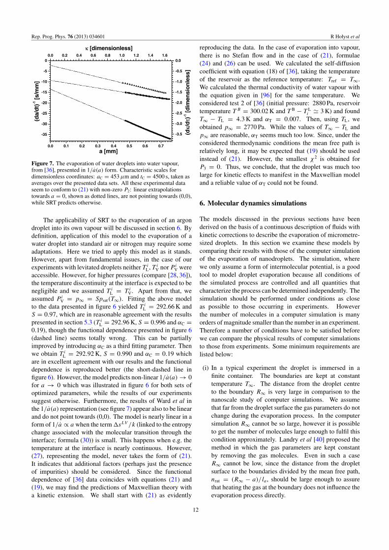
Figure 7. The evaporation of water droplets into water vapour,from [36], presented in 1/a(a) form. Characteristic scales fordimensionless coordinates: aC = 453 µm and tC = 4500 s, taken asaverages over the presented data sets. All these experimental dataseem to conform to (21) with non-zero P2: linear extrapolationstowards a = 0, shown as dotted lines, are not pointing towards (0,0),while SRT predicts otherwise.
The applicability of SRT to the evaporation of an argondroplet into its own vapour will be discussed in section 6. Bydefinition, application of this model to the evaporation of awater droplet into standard air or nitrogen may require someadaptations. Here we tried to apply this model as it stands.However, apart from fundamental issues, in the case of ourexperiments with levitated droplets neither T i
L, T iV nor P i
V wereaccessible. However, for higher pressures (compare [28, 36]),the temperature discontinuity at the interface is expected to benegligible and we assumed T i
L = T iV. Apart from that, we
assumed P iV = p∞ = Spsat(T∞). Fitting the above model
to the data presented in figure 6 yielded T iL = 292.66 K and
S = 0.97, which are in reasonable agreement with the resultspresented in section 5.3 (T i
L = 292.96 K, S = 0.996 and αC =0.19), though the functional dependence presented in figure 6(dashed line) seems totally wrong. This can be partiallyimproved by introducing αC as a third fitting parameter. Thenwe obtain T i
L = 292.92 K, S = 0.990 and αC = 0.19 whichare in excellent agreement with our results and the functionaldependence is reproduced better (the short-dashed line infigure 6). However, the model predicts non-linear 1/a(a) → 0for a → 0 which was illustrated in figure 6 for both sets ofoptimized parameters, while the results of our experimentssuggest otherwise. Furthermore, the results of Ward et al inthe 1/a(a) representation (see figure 7) appear also to be linearand do not point towards (0,0). The model is nearly linear in aform of 1/a ∝ a when the term �sLV /k (linked to the entropychange associated with the molecular transition through theinterface; formula (30)) is small. This happens when e.g. thetemperature at the interface is nearly continuous. However,(27), representing the model, never takes the form of (21).It indicates that additional factors (perhaps just the presenceof impurities) should be considered. Since the functionaldependence of [36] data coincides with equations (21) and(19), we may find the predictions of Maxwellian theory witha kinetic extension. We shall start with (21) as evidently
reproducing the data. In the case of evaporation into vapour,there is no Stefan flow and in the case of (21), formulae(24) and (26) can be used. We calculated the self-diffusioncoefficient with equation (18) of [36], taking the temperatureof the reservoir as the reference temperature: Tref = T∞.We calculated the thermal conductivity of water vapour withthe equation given in [96] for the same temperature. Weconsidered test 2 of [36] (initial pressure: 2880 Pa, reservoirtemperature T B = 300.02 K and T B − T L
i � 3 K) and foundT∞ − TL = 4.3 K and αT = 0.007. Then, using TL, weobtained p∞ = 2770 Pa. While the values of T∞ − TL andp∞ are reasonable, αT seems much too low. Since, under theconsidered thermodynamic conditions the mean free path isrelatively long, it may be expected that (19) should be usedinstead of (21). However, the smallest χ2 is obtained forP3 = 0. Thus, we conclude, that the droplet was much toolarge for kinetic effects to manifest in the Maxwellian modeland a reliable value of αT could not be found.
6. Molecular dynamics simulations
The models discussed in the previous sections have beenderived on the basis of a continuous description of fluids withkinetic corrections to describe the evaporation of micrometre-sized droplets. In this section we examine these models bycomparing their results with those of the computer simulationof the evaporation of nanodroplets. The simulation, wherewe only assume a form of intermolecular potential, is a goodtool to model droplet evaporation because all conditions ofthe simulated process are controlled and all quantities thatcharacterize the process can be determined independently. Thesimulation should be performed under conditions as closeas possible to those occurring in experiments. Howeverthe number of molecules in a computer simulation is manyorders of magnitude smaller than the number in an experiment.Therefore a number of conditions have to be satisfied beforewe can compare the physical results of computer simulationsto those from experiments. Some minimum requirements arelisted below:
(i) In a typical experiment the droplet is immersed in afinite container. The boundaries are kept at constanttemperature T∞. The distance from the droplet centreto the boundary R∞ is very large in comparison to thenanoscale study of computer simulations. We assumethat far from the droplet surface the gas parameters do notchange during the evaporation process. In the computersimulation R∞ cannot be so large, however it is possibleto get the number of molecules large enough to fulfil thiscondition approximately. Landry et al [40] proposed themethod in which the gas parameters are kept constantby removing the gas molecules. Even in such a caseR∞ cannot be low, since the distance from the dropletsurface to the boundaries divided by the mean free path,nrat = (R∞ − a)/ la , should be large enough to assurethat heating the gas at the boundary does not influence theevaporation process directly.
12
Rep. Prog. Phys. 76 (2013) 034601 R Hołyst et al
(ii) In a typical experiment the droplet radius is equal toa few micrometres. As a result, the influence of thewidth of the interface on time evolution is very low. Theresulting minimum requirement for the simulation is thatthe droplet radius should be much larger than the width ofthe interface. Considering the values of the surface widthparameter for the Lennard-Jones (LJ) liquid [97], we canassume that a should not be significantly lower than 10σ
where σ is the LJ length parameter.(iii) In experiment a/R∞ can be set to 0, while this value
is finite in computer simulations. Therefore we have toaccount for the finite size of the system in any comparisonwith experiment.
The above conditions ((i) and (ii)) are fulfilled only ifthe total number of molecules N in the simulation is large.Most simulations that can be found in the literature concern theevaporation of very small LJ droplets [40, 98, 99]. The resultswere very interesting but N , not higher than a few thousand,was much too low to fulfil both (i) and (ii). Walther andKoumoutsakos [41] (WK) performed simulations where N wasan order of magnitude larger. They modelled the evaporation ofthe LJ atom droplet at supercritical conditions and concludedthat the temporal evolution of droplet radius a(t) obeys theclassical ‘D2 evaporation law’ (as (7) or (12)):
da2
dt= const. (32)
They used formula (11) under the condition of Le = 1 to fittheir data. The number of LJ atoms in the droplet applied byWK was enough to satisfy the condition (ii). The simulationbox was also large, but nrat amounted only to about 2, whichseems to be too low.
Hołyst and Litniewski [25] (HL) have presented the resultsof large scale (N over 2.6 × 10⁶) computer simulations ofevaporation of the LJ liquid droplet surrounded by the vapour,all enclosed in a spherical vessel of radius R∞ � la . Theboundaries were kept at the constant temperature T∞ > Tc
where Tc was the critical temperature. The evaporation wassimulated for different conditions with TL/Tc varying from0.678 to 0.955. The total number of LJ atoms was large enoughto satisfy both (i) and (ii). R∞/a was always larger than 7and nrat was never lower than 10. HL have also proposedhow to take into account the finite size of the gas container(condition 3). In a typical experiment the heat is transferredfrom R∞ to the droplet surface and R∞ is so large that a/R∞can be assumed to be 0. In computer simulations R∞ is notso large and its value influences the obtained results. Theinfluence can be taken into account as in the hydrodynamicmodel [28, 32] in which the result of the integration of theheat transport equation (HTE), as e.g. (8), depends on theboundaries: both on a and on R∞. Simplifying HTE [28],the ‘D2 law’ ((32)) is fulfilled only if a/R∞ → 0. On theother hand, (32) is fulfilled for all R∞ > a if we replace a
with [25]:
a∗ = a
(1 − 2a
3R∞
)1/2
. (33)
This result strongly suggests that if a/R∞ cannot be neglected,the time evolution of the droplet radius of an experimental
system is better described by a∗(t) than a(t). In this way wesatisfy condition (iii) which is necessary to compare the resultsof experiments to those of computer simulations.
In the following, we use the computer simulation data fromthe HL work (listed in table I in [25]) to test the theoreticalformulae for da∗/dt . In the simulations, a was defined as thedistance from the droplet mass centre to the point where thedensity is equal to half of the mean density of the droplet.All the results given below are expressed in units of argonassuming the mass m = 40 a.m.u. and the LJ parameters: σ =3.4×10⁻¹⁰ m, ε = 140.5k = 1.939×10⁻²¹ J. The temperaturescale is obtained by adopting the critical temperature for theLJ potential truncated at rc = 2.5σ (Tc = 1.08 in the reducedunits [97]) equal to the temperature for argon (151.75 K).
Using the computer simulation data of HL [25] weestimated the gas density just above the droplet surface ρa . Wedetermined the diffusion coefficient in the vapour D and theheat capacity cp for the gas density ρa by performing additionalshort computer simulations on the 125 000 particle systemsusing the constant energy and volume molecular dynamics(MD) method [100]. The values of D at ρa , further denoted asDa , were determined using the Einstein formula [100] for allvalues of liquid temperature considered here. The specificheat has been estimated for two state points: cp = 2.8R
for ρ/m = 0.165 nm−3, T = 102.7 K and cp = 3.7R
for ρ/m = 0.832 nm−3, T = 128.1 K. The values of cp
together with λ from the supplementary information to theHL paper [25] gives Le = 1.06 and 0.92, respectively, whichshows that in our case, the assumption Le ≈ 1 is a reasonableapproximation.
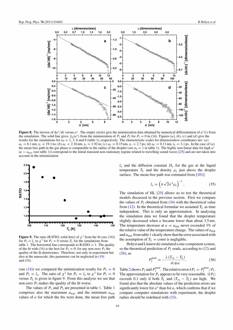
First, an important result that we have found analysingthe simulation data is that the time evolution of the inverse ofda∗/dt in a quasi-stationary regime (the second part of the timeevolution) is a strictly linear function of a∗ (formula (21)). Wefitted (da∗/dt)−1 with the function ffit(a
∗) being the inverseof the general formula (19):(
da∗
dt
)−1
= ffit(a∗) = − 1
P1
(a∗
1 + P3/a∗ + P2
), (34)
where now P1, P2 and P3 � 0 are adjustable constants. Thecurves resulted from the minimization for selected data areshown in figure 8 ((da∗/dt)−1 versus a∗). Initially (largea∗ in figure 8) the system was heated at the boundary anda sudden change of temperature resulted in sound wavestravelling in the system. For this time period (34) was notvalid. For the rest of the time, the evaporation process waswell described by the linear dependence of (da∗/dt)−1 versusa∗ (figure 8). According to (33) da∗/dt = (da/dt)[1 −2a/(3R∞) + O(a2/R2
∞)]. The differences in the quality ofthe fit (determined by χ2) for (da/dt)−1 and (da∗/dt)−1 werenon-significant. The only, physically important, differencewas that the values of P1 for a∗ were higher than that for a by 13to 20% of the relative value. The presence of P3 in (34) did notimprove the quality of the fit. For the temperature of the liquiddroplet TL < 122 K the minimization always gave P3 = 0. Forlarger TL, P3 was usually non-zero but the difference betweenthe corresponding χ2 and that for P3 = 0 was always non-significant. Following the discussion on the meaning of �C
13
Rep. Prog. Phys. 76 (2013) 034601 R Hołyst et al
Figure 8. The inverse of da∗/dt versus a∗. The empty circles give the minimization data obtained by numerical differentiation of a∗(t) fromthe simulation. The solid line gives ffit(a
∗) from the minimization of P1 and P2 for P3 = 0 in (34). Figures (a), (b), (c) and (d) give theresults for the simulations for n0 = 1, 3, 6 and 8 (table 1), respectively. The characteristic scales for dimensionless coordinates are: (a)aC = 6.1 nm, tC = 19.1 ns; (b) aC = 2.16 nm, tC = 1.92 ns; (c) aC = 0.15 nm, tC = 2.7 ps; (d) aC = 0.11 nm, tC = 3.1 ps. In the case of (a)the mean free path in the gas phase is comparable to the radius of the droplet (see n0 = 1 in table 1). The highly non-linear data for high a∗
(a > amax (see table 1)) correspond to the initial transient non-stationary regime related to travelling sound waves [25] and are not taken intoaccount in the minimization.
L
Figure 9. The ratio (RATIO; solid dots) of χ2 from the fit (see (34))for P3 = la to χ 2 for P3 = 0 versus TL for the simulations fromtable 1. The horizontal line corresponds to RATIO = 1. The qualityof the fit with (34) is the best for P3 = 0; for any non-zero P3 thequality of the fit deteriorates. Therefore, not only in experiment butalso at the nanoscale, this parameter can be neglected in (19)and (34).
(see (14)) we compared the minimization results for P3 = 0and P3 = la . The ratio of χ2 for P3 = la to χ2 for P3 = 0versus TL is given in figure 9. From this analysis we see thatnon-zero P3 makes the quality of the fit worse.
The values of P1 and P2 are presented in table 1. Table 1comprises also the maximum amax and the minimum amin
values of a for which the fits were done, the mean free path
la and the diffusion constant Da for the gas at the liquidtemperature TL and the density ρa just above the dropletsurface. The mean free path was estimated from [101]:
la =(π
√2σ 2ρa
)−1. (35)
The simulation of HL [25] allows us to test the theoreticalmodels discussed in the previous section. First we comparethe values of P1 obtained from (34) with the theoretical valuefrom (12). In the theoretical formulae we assumed TL as timeindependent. This is only an approximation. In analysingthe simulation data we found that the droplet temperatureslightly decreased when a became lower than about 3.5 nm.The temperature decrease at a = amin never exceeded 3% ofthe relative value of the temperature change. The values of amin
and amax from table 1 clearly show that the error associated withthe assumption of TL = const is negligible.
Hołyst and Litniewski simulated a one-component system,so the theoretical prediction of P1 reads, according to (12) and(26), as
Ppred1 = −λ (T∞ − TL)
ρLqeff. (36)
Table 2 showsP1 andPpred1 . The relative error δP1 = P
pred1 /P1.
The approximation for P1 appears to be very reasonable. |δP1|exceeds 0.1 only if both TL and (T∞ − TL) are high. Wefound also that the absolute values of the prediction errors aresignificantly lower for a∗ than for a, which confirms that if wecompare computer simulations with experiment, the dropletradius should be redefined with (33).
14

Rep. Prog. Phys. 76 (2013) 034601 R Hołyst et al
Table 1. The computer simulation data, the minimization results and the parameters for the simulations from [25]. The sequence numbersn0 correspond to those from table 1 of [25]. P1 and P2 (see equations (21) and (19)) are obtained from the minimization of ffit(a
∗) (formula(34)) for P3 = 0. ρa is the density of gas close to the droplet surface and Da is the diffusion coefficient obtained from the simulation at ρa
and TL. TL is the liquid droplet temperature during evaporation (almost constant as explained in the body of the text) and ρL is the liquidmass density. T∞ is the temperature at the boundary of the container. amin and amax give the minimum and maximum values of the dropletradius a used during the minimization (see also figure 8) and la is the mean free path in the gas phase evaluated from (35).
TL T∞ ρL/m ρa/m Da P2 P1 la amin amax
n0 (K) (K) (nm−3) (nm−3) (mm2 s−1) (nm) (nm2 ns−1) (nm) (nm) (nm)
1 102.7 175.6 19.7 0.216 0.726 6.10 1.95 9.00 3.2 11.42 107.9 175.6 19.2 0.318 0.517 3.41 2.07 6.12 2.4 11.03 114.6 175.6 18.5 0.496 0.349 2.16 2.43 3.92 2.5 10.34 121.3 175.6 17.7 0.725 0.252 1.03 2.67 2.69 2.1 7.75 128.1 175.6 16.8 1.119 0.174 0.21 2.98 1.74 2.3 7.96 135.3 245.9 15.8 1.399 0.145 0.15 8.46 1.39 2.6 7.37 142.9 351.3 14.4 1.743 0.123 −0.03 16.90 1.12 2.4 8.08 136.4 175.6 15.6 1.705 0.122 0.11 3.93 1.14 2.5 10.29 144.9 245.9 13.8 2.099 0.104 0.01 13.12 0.93 3.4 9.7
Table 2. The comparison of P1 from the minimization with ffit(a∗)
(see table 1) and the theoretical value of P1 (P pred1 from formula
(36)). The approximation for P1 appears to be very reasonable. Therelative error in P
pred1 exceeds 0.1 only if both TL and T∞ − TL
are high.
TL T∞ − TL P1 Ppred1
n0 (K) (K) (nm2 ns−1) (nm2 ns−1)
1 102.7 72.9 1.95 2.092 107.9 67.7 2.07 2.213 114.6 61.0 2.43 2.454 121.3 54.4 2.67 2.725 128.1 47.5 2.98 3.056 135.3 110.6 8.46 8.247 142.9 208.4 16.90 19.298 136.4 39.2 3.93 3.549 144.9 101.0 13.12 12.01
As it has been already mentioned, SRT predicts a in aform different from (19). Table 3 compares a from the MDsimulation with that predicted by SRT for a = 20σ = 6.8 nm.SRT predicts a non-physical result: aSRT is positive i.e. thedroplet grows in time instead of decreasing its size. For theconditions given in table 3, pV is significantly higher thanpsat(TL). The first term in formula (30) becomes stronglynegative and �sLV/k changes sign. It may be confirmed byan observation that significantly better results are obtained bysetting up false pV = psat(TL). Then, the prediction given byaSRTEQ is not so poor if only TL is low enough. SRT seems togain accuracy for moderately non-equilibrium processes (seeT∞ − TL in table 2).
We are not aware of any theory that predicts the valueof P2 successfully in the whole range of temperatures anddensities. Assuming Le ≈ const, (26) predicts P2 proportionalto DaT
−1/2. Taking into account (35), the assumption that P2
is proportional to la/a [25] gives a very similar relation sinceρaDaT
−1/2 is a very weakly changing quantity (see table 1).In fact, the dependence of P2 on thermodynamic variables ismore complex. Assuming Le = 1, (26) gives, the followingrelation between αT and P2:
αT = Da
P2
√2πM/(RTL). (37)
According to figure 9, αT calculated from formula (37)as a function of ρa splits into two regions, those of highand low values. An important result that we have foundwhen analysing the simulation data is that the jump in α−1
T ,which is seen in figure 10, is strictly correlated with thetemperature discontinuity at the droplet surface that is shownin the HL paper [25]. The effect is evident if we comparethe two panels of figure 10. Therefore we conclude that thehigh value of α−1
T found in experiments is a sign that kineticeffects are important and that their origin is in the temperaturediscontinuity measured for the first time by. Ward and hisgroup [13]. For the continuous profile of the temperatureacross the interface P2 = 0 and consequently α−1
T = 0.
7. Summary
The temporal evolution of the radius of evaporating dropletsfollows (21), irrespective of whether it pertains to a singlecomponent (evaporation of the liquid into its own vapour)or multi-component system (evaporation of a liquid into agas or vapour of another substance). This equation has twoparameters: P1 and P2. P1 is well described by the continuousirreversible thermodynamics approach in the form of formulae(24) or (26). P2 is a correction arising from the kinetic theoryof gases (again, see formulae (24) and (26)). The form of P2
involves unknown evaporation coefficients. In the case of anevaporation of a liquid into its own vapour, P2 is non-zero onlyif there is a temperature discontinuity at the interface.
The temperature discontinuity appears always for asufficiently small density of the vapour phase. This factindicates that the temperature jump at the interface is dueto the momentum/pressure equilibrium. The explanationis very simple: for diluted vapour the pressure is givenby the product of the vapour density and temperature. Ifthe density is too low, only sufficiently high temperatureswould guarantee momentum/pressure equilibrium. Thusequilibration of pressures (including the curvature term inthe Laplace law for droplets) during evaporation is the mainmechanism for the temperature discontinuity at the liquid–vapour interface.
15

Rep. Prog. Phys. 76 (2013) 034601 R Hołyst et al
Table 3. The comparison of a for a = 6.8 nm from the HL simulation (index sim) with the value from the SRT model for pV from the MDsimulation and for the assumption of pV = psat(TL) (indices SRT and SRTEQ, respectively). The surface tension γ and the saturation pressurepsat(TL) are taken from [97].
TL γ psat(TL) pV asim aSRT aSRTEQ
n0 (K) (mJ m−2) (MPa) (MPa) (nm ns−1) (nm ns−1) (nm ns−1)
1 102.7 8.26 0.340 0.414 −0.151 0.168 −0.1342 107.9 7.10 0.502 0.597 −0.203 0.220 −0.1643 114.7 5.68 0.789 0.893 −0.271 0.222 −0.2014 121.3 4.26 1.171 1.327 −0.341 0.406 −0.2215 128.1 2.96 1.693 1.840 −0.425 0.374 −0.2236 135.3 1.84 2.389 2.664 −1.218 0.898 −0.2037 142.9 0.83 3.315 3.774 −2.495 1.710 −0.1418 136.4 1.55 2.514 2.649 −0.568 0.378 −0.1839 144.9 0.64 3.588 3.897 −1.927 1.172 −0.123
(a)
(b)
Figure 10. (a) The inverse of αT constant calculated from (37) as afunction of the gas density above the interface, ρa . The vales of P2
are taken from table 1. αT parameter is usually assumed constant inexperimental studies. Here we show that its value depends on thegas density and therefore can vary from system to system dependingon the thermodynamic parameters of the vapour phase. For a largevapour density this parameter becomes infinitely large which meansthat the concept of kinetic-limited transport (the ballistic motion ofmolecules) is not adequate. For lower values of ρa , the value of αT
is much more reasonable however the parameter cannot be simplyinterpreted as the probability [45]. Moreover the change of αT iscorrelated with the discontinuity of temperature at the interface. Forα−1
T ≈ 0 the temperature is continuous at the interface (seefigure 10). As αT is related to the kinetic-limited transport weconclude that such transport significantly affects evaporation onlyfor a low gas density correlated with temperature discontinuity at theinterface. Such behaviour is characteristic for most experimentalcases as discussed in the experimental section and as shown in theexperiments of Ward [13, 36]. (b) Open circles: the differencebetween the liquid temperature TL and the gas temperature at theinterface Tvap (temperature jump at the interface, see [25]) as afunction of the vapour density ρa . Solid dots: the temperature jumpat the interface is inversely proportional to the density of the vapourphase (below some characteristic density in the system as shown inthe figure). For a sufficiently high vapour density the temperature iscontinuous at the interface i.e. TL = Tvap.
The evaporation is in the first place driven by the heatflux from the vapour phase. However lowering the vapourdensity would finally lead to the evaporation scenario beingcompletely dominated by kinetic effects (not fully accountedfor by formulae (26), where the kinetic term is only the
correction to the main part). An extreme case is evaporationinto vacuum, when the momentum flux density is equal to theliquid pressure and governs in this way the mass flux [26, 27].In the latter case there is no heat flux from outside and duringevaporation the droplet lowers its temperature.
For multi-component systems the situation is different andthe scenario of evaporation changes, despite the fact that thesame (21) is valid as in the single-component system. Firstof all the vapour has high density and momentum/pressureequilibrium is satisfied easily e.g. for water evaporating intothe air. Therefore momentum/pressure equilibrium is not theconstraint which governs density and temperature profiles as inthe single-component system. We believe that the scenario ofevaporation is as follows: the droplet is originally at the sametemperature as the vapour/ambient atmosphere. After a shorttime the droplet lowers in temperature because of evaporationuntil the heat flux from the surrounding gas matches theenthalpy of evaporation. The temperature difference betweenthe gas and the droplet is usually small and most probablythe temperature is simply discontinuous at the interface. Thetemperature difference between the vapour and the dropletis defined by the evaporation mass flux and enthalpy ofevaporation. The mass flux is most probably given by (13)once again with an unknown evaporation coefficient αC.
It is feasible to find a reliable value of αC (if necessarycorrected for a higher droplet temperature drop). The resultswe obtained for water versus temperature are in excellentagreement with those obtained with a fundamentally differentmethod of the BC/ARI group. The value of αT is significantlylower than obtained with a multi-parameter fit and by mostauthors. Therefore we conclude that the problem of theevaporation coefficient is still open especially because thereis no consistent theory which would explain its origin. Theevaporation coefficients should be explained on the basisof equilibrium simulations of liquids in contact with theirvapours. The experiments of Davidovits (see e.g. [66]) showthat αC is smaller than 1. It is not a surprise because the fluxleaving the liquid surface is matched by a flux which reachesthe surface of the liquid and is not reflected. If we take aclassical Hertz–Knudsen equation for the mass flux, it shouldbe multiplied by a factor which cuts out the flux that is reflectedat the interface.
The experiments yield a number of specific conclusions:Accounting for kinetic effects is indispensable for droplets of
16

Rep. Prog. Phys. 76 (2013) 034601 R Hołyst et al
the radius a < 5 µm evaporating into a standard atmosphere,regardless of the evaporation rate. Neither a diffusion only,nor kinetic only approach is successful. As long as 1/a(a) islinear, it is sufficient to use the transport equations as given by(21). �C and �T can be neglected. Such a method is simpleand quick. Accounting for the effects of temperature changewith time turned out to be not necessary even for relativelyfast evaporating droplets. The effect of surface tension issubstantial only for the droplets evaporating into their ownnearly saturated vapour. In dealing with pure liquids, theeffects of impurities can be avoided by careful handling duringexperiment and using the strictly linear region of 1/a(a) dataduring data processing. It is possible to find the value ofp∞ (or relative humidity) and (possibly) TL with the accuracydetermined mostly by the accuracy of T∞. As long as the modelis correct it is a method of remote temperature and humiditymeasurement.
Finally we have investigated in detail the SRT theoryof Ward et al [23]. According to experimental resultsand computer simulations the theory needs some revisions.However, it seems to gain accuracy for moderately non-equilibrium processes. In particular SRT does not reduce to(21) which describes correctly the evaporation in single- andmulti-component systems.
We conclude that it is indispensable for further progressin the physics of evaporation to run large scale moleculardynamics simulations at equilibrium to determine theevaporation coefficients αC and αT and relate them tointermolecular potential and thermodynamic parameters (seerecent [102]). These coefficients affect the coefficient P2 in(21) in the case of evaporation in a single-component system(see also equations (24) and (26)) and also the temperaturedifference in (26) (and consequently P1) in the case ofevaporation in a multi-component system. They are alsoimportant for the description of the smooth transition betweenthe case of evaporation into the vapour of high pressure andthe evaporation into vacuum, where it has been exactly shown[26, 27] that αC = 2 in (13). The current paradigm in scienceis focused on states rather than processes themselves, but mostcertainly the future belongs to the latter. We hope that ourmanuscript can guide future studies in this direction.
Acknowledgments
This work was supported by the Ministry of Science and HigherEducation/European Science Foundation (ESF/PESC EPSDprogram) as a scientific project 2010–2013 and by the PolishMinistry of Science and Higher Education under grant noN N202 126837. We would also like to acknowledge the usefuldiscussions with Piotr Flatau on the evaporation of oceans. Wealso acknowledge discussions with Charles Ward on SRT andthe temperature jump at the interface.
Reference
[1] Roderick M L, Hobbins M T and Farquhar G D 2009 Panevaporation trends and the terrestrial water balance: II.Energy balance and interpretation Geography Compass3 761–80
[2] Sazhin S S 2006 Advanced models of fuel droplet heatingand evaporation Prog. Energy Combust. Sci. 32 162–214
[3] Valero F P J, Collins W D, Pilewskie P, Bucholtz A andFlatau P J 1997 Direct radiometric observations of thewater vapor greenhouse effect over the equatorial pacificocean Science 275 1773–6
[4] Penman H L 1947 Evaporation in nature Rep. Prog. Phys.11 366–88
[5] Seto J, Tomine K, Wakimizu K and Nishiyama K 2011Artificial cloud seeding using liquid carbon dioxide:comparisons of experimental data and numerical analysesJ. Appl. Meteor. Climatol. 50 1417–31
[6] Wheeler T D and Stroock A D 2008 The transpiration ofwater at negative pressures in a synthetic tree Nature455 208–12
[7] Sorensen J G and Holmstrup M 2011 Cryoprotectivedehydration is widespread in arctic springtails J. InsectPhysiol. 57 1147–53
[8] Chaker M and Meher-Homji C B 2011 Gas turbine poweraugmentation: parametric study relating to fog droplet sizeand its influence on evaporative efficiency J. Eng. GasTurbines Power 133 092001
[9] Singh G, Pillai P, Arpanaei A and Kingshott P 2011Layer-by-layer growth of multicomponent colloidalcrystals over large areas Adv. Funct. Mater. 21 2556–63
[10] Dragnevski K I, Routh A F, Murray M W and Donald A M2010 Cracking of drying latex films: an ESEM experimentLangmuir 26 7747–51
[11] Dragnevski K I and Donald A M 2008 An environmentalscanning electron microscopy examination of the filmformation mechanism of novel acrylic latex Colloids Surf.A 317 551–6
[12] Dessler A E and Sherwood S C 2009 A matter of humidityScience 323 1020–21
[13] Fang G and Ward C A 1999 Temperature measured close tothe interface of an evaporating liquid Phys. Rev. E59 417–28
[14] Pao Y-P 1971 Application of kinetic theory to theproblem of evaporation and condensation Phys. Fluids14 306–12
[15] Pao Y-P 1971 Temperature and density jumps in thekinetic theory of gases and vapors Phys. Fluids14 1340–6
[16] Pao Y-P 1973 Temperature and density jumps in the kinetictheory of gases and vapors Phys. Fluids 16 1560
[17] Cipolla J W Jr, Lang H and Loyalka S K 1974 Kinetic theoryof condensation and evaporation: II J. Chem. Phys.61 69–77
[18] Bedaux D, Hermans L F and Ytrehus T 1990 Slowevaporation and condensation Physica A: Stat. Mech.Appl. 169 263–80
[19] Young J B 1991 The condensation and evaporation of liquiddroplets in a pure vapour at arbitrary knudsen number Int.J. Heat. Transfer 34 1649–61
[20] Maxwell J C 1879 On stresses in rarefied gases arising frominequalities of temperature Phil. Trans. R. Soc. Lond.170 231–56
[21] Persad A H and Ward C A 2010 Statistical rate theoryexamination of ethanol evaporation J. Chem. Phys. B114 6107–16
[22] Bond M and Struchtrup H 2004 Mean evaporation andcondensation coefficients based on energy dependentcondensation probability Phys. Rev. E 70 061605
[23] Ward C A and Fang G 1999 Expression for predicting liquidevaporation flux: statistical rate theory approach Phys.Rev. E 59 429–40
[24] Das K S, MacDonald C A and Ward B D 2010 Stability ofevaporating water when heated through the vapor and theliquid phases Phys. Rev. E 81 036318
17

Rep. Prog. Phys. 76 (2013) 034601 R Hołyst et al
[25] Hołyst R and Litniewski M 2008 Heat transfer at thenanoscale: evaporation of nanodroplets Phys. Rev. Lett.100 055701
[26] Hołyst R and Litniewski M 2009 Evaporation into vacuum:mass flux from momentum flux and the hertz–knudsenrelation revisited J. Chem. Phys. 130 074707
[27] Cheng S, Lechman J B, Plimpton S J and Grest G S 2011Evaporation of Lennard-Jones fluids J. Chem. Phys.134 224704
[28] Babin V and Hołyst R 2005 Evaporation of a sub-micrometerdroplet J. Phys. Chem. B 109 11367–72
[29] Babin V and Hołyst R 2005 Evaporation of a thin liquid filmJ. Chem. Phys. 122 024713
[30] Ward C A and Stanga D 2001 Interfacial conditions duringevaporation or condensation of water Phys. Rev. E64 051509
[31] Maxwell J C 1890 Collected Sci. Papers 11 625[32] Sirignano W A 2010 Fluid Dynamics and Transport of
Droplets and Sprays (Cambridge: Cambridge UniversityPress)
[33] Hirschfelder J O, Curtiss C F and Bird R B 1954 MolecularTheory of Gases and Liquids (New York: Wiley)
[34] Fukuta N and Myers M N 2007 Simultaneous measurementof condensation and thermal accommodation coefficientsfor cloud droplet growth in due consideration of a newmoving surface-boundary effect J. Atmos. Sci. 64 955–68
[35] Fuchs N A 1959 Evaporation and Droplet Growth inGaseous Media (London: Pergamon)
[36] McGaughey A J H and Ward C A 2002 Temperaturediscontinuity at the surface of an evaporating dropletJ. Appl. Phys. 91 6406–15
[37] Friedlander S K 2000 Smoke, Dust and Haze Fundamentalsof Aerosol Dynamics (New York Oxford: OxfordUniversity Press)
[38] Pruppacher H R and Klett J D 1997 Microphysics of Cloudsand Precipitation (Dordrecht: Kluwer)
[39] Jakubczyk D, Zientara M, Kolwas K and Kolwas M 2007Temperature dependence of evaporation coefficient forwater measured in droplets in nitrogen under atmosphericpressure J. Atmos. Sci. 64 996–1004
[40] Landry E S, Mikkilineni S, Paharia M and McGaughey A J H2007 Droplet evaporation: a molecular dynamicsinvestigation J. Appl. Phys. 102 124301
[41] Walther J H and Koumoutsakos P 2001 Molecular dynamicssimulation of nanordoplet evaporation J. Heat Transfer123 741–8
[42] Langmuir I J 1915 The dissociation of hydrogen into atoms:II. Calculation of the degree of dissociation and the heat offormation J. Am. Chem. Soc. 37 417–58
[43] Zientara M, Jakubczyk D, Kolwas K and Kolwas M 2008Temperature dependence of the evaporation coefficient ofwater in air and nitrogen under atmospheric pressure:study in water droplets J. Phys. Chem. A 112 5152–8
[44] Smith J D, Cappa C D, Drisdell W S, Cohen R C andSaykally R J 2006 Raman thermometry measurements offree evaporation from liquid water droplets J. Am. Chem.Soc. 128 12892–8
[45] Knudsen M 1950 The Kinetic Theory of Gases: SomeModern Aspects (London: Methuen)
[46] Nathanson G M, Davidovits P, Worsnop D R and Kolb C E1996 Dynamics and kinetics at the gas–liquid interfaceJ. Phys. Chem. 100 13007–20
[47] Bagot P A J, Waring C, Costen M L and McKendrick K G2008 Dynamics of inelastic scattering of oh radicals fromreactive and inert liquid surfaces J. Phys. Chem. C112 10868–77
[48] Drisdell W S, Cappa C D, Smith J D, Saykally R J andCohen R C 2008 Determination of the evaporationcoefficient of D2O Atmos. Chem. Phys. 8 6699–706
[49] McFeely F R and Somorjai G A 1972 Studies of vaporizationkinetics of hydrogen-bonded liquids J. Phys. Chem.76 914–8
[50] Frezzotti A, Gibelli L and Lorenzani S 2005 Mean fieldkinetic theory description of evaporation of a fluid intovacuum Phys. Fluids 17 012102
[51] Carey V P and Wemhoff A P 2004 Relationships amongliquid–vapor interfacial region properties: predictions of athermodynamic model Int. J. Thermophys. 25 753–86
[52] Ford I J and Lee T-L 2001 Entropy production anddestruction in models of material evaporation J. Phys. D:Appl. Phys. 34 413–7
[53] Bellomo N and Chiado Piat M G 1975 Liquid dropletsvaporization gas beam conditions Meccanica 10 57–60
[54] Winkler P M, Vrtala A, Wagner P E, Kulmala M,Lehtinen K E J and Vesala T 2006 Condensation of watervapor: experimental determination of mass and thermalaccommodation coefficients J. Geophys. Res. 111 D19202
[55] Li Y Q, Davidovits P, Shi Q, Jayne J T, Kolb C E andWorsnop D R 2001 Mass and thermal accommodationcoefficients of H2O (g) on liquid water as function oftemperature J. Phys. Chem. A 105 10627–34
[56] Winkler P M, Vrtala A, Wagner P E, Kulmala M,Lehtinen K E J and Vesala T 2004 Mass and thermalaccommodation during gas-liquid condensation of waterPhys. Rev. Lett. 93 75701
[57] Hagen D E, Schmitt J, Trublood M, Carstens J, White D Rand Alofs D J 1989 Condensation coefficient measurementfor water in the UMR cloud simulation chamber J. Atmos.Sci. 46 803–16
[58] Zagaynow V A, Nuzhny V M, Cheeusova T A andLushnikov A A 2000 Evaporation of water droplet andcondensation coefficient: theory and experiment J. AerosolSci. 31 (Suppl.) 1 S795–6
[59] Sageev G, Flagan R C, Seinfeld J H and Arnold S 1986Condensation of water on aqueous droplets in thetransition regime Colloid Interface Sci. 113 421–9
[60] Gollub J P, Chabay I and Flygare W H 1974 Laser heterodynestudy of water droplet growth J. Chem. Phys. 61 2139–44
[61] Shaw R A and Lamb D 1999 Experimental determination ofthe thermal accommodation and condensation coefficientsof water J. Chem. Phys. 111 10659–63
[62] Xue H, Moyle A M, Magee N, Harrington J Y and Lamb D2005 Experimental studies of droplet evaporation kinetics:validation of models for binary and ternary aqueoussolutions J. Atmos. Sci. 62 4310–26
[63] Davis E J 2006 A history and state-of-the-art ofaccommodation coefficients Atmos. Res. 82 561–78
[64] Marek R and Straub J 2001 Analysis of the evaporationcoefficient and the condensation coefficient of water Int. J.Heat Mass Transfer 44 39–53
[65] Eames L W, Marr N J and Sabir H 1997 The evaporationcoefficient of water: a review Int. J. Heat and MassTransfer 40 4522–9
[66] Davidovits P et al 2004 Mass accommodation coefficient ofwater vapor on liquid water Geophys. Res. Lett.31 L22111
[67] Kirchner W, Welter F, Bongartz A, Kames J,Schweighoefer S and Schurath U 1990 Trace gas exchangeat the air/water interface: measurements of massaccommodation coefficients J. Atmos. Chem. 10 427–49
[68] Rudolf R, Vrtala A, Kulmala M, Vesala T and Wagner P E2000 Experimental study of sticking probabilities forcondensation of nitric acid-water vapor mixtures AerosolSci. 32 913–32
[69] Schwartz S E and Freiberg J E 1981 Mass-transportlimitation to the rate of reaction of gases in liquid droplets:application to oxidation of SO2 in aqueous solutionsAtmos. Environ. 15 1129–44
18
Rep. Prog. Phys. 76 (2013) 034601 R Hołyst et al
[70] Shi Q, Davidovits P, Jayne J T, Worsnop D R and Kolb C E1999 Uptake of gas-phase ammonia: I. Uptake by aqueoussurfaces as a function of ph J. Phys. Chem. A 103 8812–23
[71] Worsnop D R, Zahniser M S, Kolb C E, Gardner J A,Watson L R, Van Doren J M, Jayne J T and Davidovits P1989 Temperature dependence of mass accommodation ofSO2, and H2O2 on aqueous surfaces J. Phys. Chem.93 1159–72
[72] Jayne J T, Duan S X, Davidovits P, Worsnop D R,Zahniser M S and Kolb C E 1991 Uptake of gas-phasealcohol and organic acid molecules by water surfacesJ. Phys. Chem. 95 6329–36
[73] Kolb C E et al 2010 An overview of current issues in theuptake of atmospheric trace gases by aerosols and cloudsAtmos. Chem. Phys. 10 10561–605
[74] Heideger W J and Boudart M 1962 Interfacial resistance toevaporation Chem. Eng. Sci. 17 1–10
[75] Lednovich S L and Fenn J B 1977 Absolute evaporation ratesfor some polar and nonpolar liquids AIChE J. 23 454–9
[76] Tsurata T, Kato Y, Yasunobu T and Masuoka T 1994Estimation of condensation coefficient by dropwisecondensation method: condensation coefficients ofethylene glycol and water Trans. Japan Soc. Mech. Eng. B60 508–14
[77] Maa J R 2001 Rates of evaporation and condensationbetween pure liquids and their own vapors Indust. Eng.Chem. Fundam. 9 283–7
[78] Chekmarev S F 1996 Effect of condensation heat on thecondensation coefficient AIChE J. 42 2467–75
[79] Narusawa U and Springer G S 1975 Measurement ofevaporation rates of water J. Colloid Interface Sci.50 392–5
[80] Jakubczyk D, Kolwas M, Derkachov G, Kolwas K andZientara M 2012 Evaporation of micro-droplets: the‘radius-square-law’ revisited Acta Phys. Polon. A 122709–16
[81] Viswanathan R, Lakshmi Narasimhan T S and Nalini S 2009Vapor pressure measurements by mass loss transpirationmethod with a thermogravimetric apparatus J. Phys.Chem. B 113 8362–8
[82] Price D M 2001 Volatilisation, evaporation and vapourpressure studies using a thermobalance J. Therm. Anal.Calorimetry 64 315–22
[83] Major F G, Gheorghe V N and Werth G 2005 ChargedParticle Traps (Berlin: Springer)
[84] Davis E J, Buehler M F and Ward T L 1990 The double-ringelectrodynamic balance for microparticle characterizationRev. Sci. Instrum. 61 1281–8
[85] Arnold S 1991 A three-axis spherical void electrodynamiclevitator trap for microparticle experiments Rev. Sci.Instrum. 62 3025–8
[86] Allison E E and Kendall B R F 1996 Cubic electrodynamiclevitation trap with transparent electrodes Rev. Sci.Instrum. 67 3806–12
[87] Dehaeck S and van Beeck J P A J 2008 Multifrequencyinterferometric particle imaging for gas bubble sizing Exp.Fluids 45 823–31
[88] Zientara M, Jakubczyk D, Derkachov G, Kolwas K andKolwas M 2005 Simultaneous determination of mass andthermal accommodation coefficients from temporalevolution of an evaporating water microdroplet J. Phys. D:Appl. Phys. 38 1978–83
[89] Jakubczyk D, Derkachov G, Do Duc T, Kolwas K andKolwas M 2010 Coefficients of evaporation and gas phasediffusion of low-volatility organic solvents in nitrogenfrom interferometric study of evaporating droplets J. Phys.Chem. A 114 3483–8
[90] Wilms J 2005 Evaporation of Multicomponent Droplets PhDThesis Universitat Stuttgart
[91] Ni P 2010 A fuel droplet vaporization model in a hot airstream Appl. Math. Modelling 34 2370–6
[92] Delle Site A 1997 The vapor pressure of environmentallysignificant organic chemicals: a review of methods anddata at ambient temperature J. Phys. Chem. Ref. Data26 157–93
[93] Lugg G A 1968 Diffusion coefficients of some organic andother vapors in air Anal. Chem. 40 1072–7
[94] The MEGlobal Group of Companies 2005 Diethylene GlycolProduct Guide www.meglobal.biz/media/product guides/MEGlobal DEG.pdf
[95] Duan F, Thompson I and Ward C A 2008 Statistical ratetheory determination of water properties below the triplepoint J. Phys. Chem. B 112 8605–13
[96] The International Association for the Properties of Water andSteam. Revised Release on the IAPWS Formulation 1985for the Thermal Conductivity of Ordinary WaterSubstance. London, England, 1998
[97] Vrabec J, Kedia G K, Fuchs G and Hasse H 2006Comprehensive study on vapour-liquid coexistence ofthe truncated and shifted lennard-jones fluid includingplanar and spherical interface properties Mol. Phys.104 1509–27
[98] Long N L, Micci M M and Wong B C 1996 Coefficients ofevaporation and gas phase diffusion of low-volatilityorganic solvents in nitrogen from interferometricstudy of evaporating droplets Comput. Phys. Commun.96 167
[99] Consolini L, Aggarwal S K and Murad S 2003 A moleculardynamics simulation of droplet evaporation Int. J. HeatMass Transfer 46 3179–88
[100] Allen M P and Tildesley D J 1987 Computer Simulations ofLiquids (Oxford: Oxford University Press)
[101] Resibois P and de Leener M 1977 Classical Kinetic Theory ofFluids (New York: Wiley)
[102] Ishiyama T, Yano T and Fujikawa S 2005 Kinetic boundarycondition at a vapor-liquid interface Phys. Rev. Lett.95 084504
19