progress in electromagnetics research

Progress In Electromagnetics Research B, Vol. 89, 87–109, 2020

Theory of Electromagnetic Radiation in Nonlocal Metamaterials —Part II: Applications

Said Mikki*

Abstract—We deploy the general momentum space theory developed in Part I in order to explorenonlocal radiating systems utilizing isotropic spatially-dispersive metamaterials. The frequency-dependent angular radiation power density is derived for both transverse and longitudinal externalsources, providing detailed expressions for some special but important cases like time-harmonic- andrectangular-pulse-excited small dipoles embedded into such isotropic metamaterial domains. Thefundamental properties of dispersion and radiation functions for some of these domains are developed inexamples illustrating the features in nonlocal radiation phenomena, including differences in bandwidthand directivity performance, novel virtual array effects, and others. In particular, we show that bya proper combination of transverse and longitudinal modes, it is possible to attain perfect isotropicradiators in domains excited by small sinusoidal dipoles. The directivity of a nonlocal small antenna isalso shown to increase by possibly four times its value in conventional local domains if certain designconditions are met.

1. INTRODUCTION

The principal goal of this paper is to demonstrate how the general momentum-space theory of Part I [1]can be deployed to help understanding the basic radiation properties of elementary sources embeddedinto such nonlocal metamaterials. Some general issues related to the overall scope of this work and thedesign of metamaterials for radiating nonlocal systems had already been discussed in the introductorysections of Part I and Sec. 5 there and the reader is referred to that material for further information.In the remaining part of this Introduction, we focus on providing a general overview of the content ofthe present paper.

We start with Sec. 2, which is dedicated to presenting the main rudimentary facts (supportedby the Appendix) about the main genre of nonlocal metamaterials considered in Part II, namely thegeneric isotropic medium whose essential features pertinent to radiation theory are briefly sketchedout in Sec. 2.1. After that, we further specialize the general isotropic case in Sec. 2.2 to concentratefor the rest of this paper on the special but substantial example of non-resonant isotropic nonlocalmetamaterials (NR-NL-MTM). In Sec. 3, we start investigating the first concrete antenna type in thispaper, a point source, dipole-like radiator embedded into the NR-NL-MTM described in the previoussection. To do so, we first need to slightly modify the previous theory to deal with continuous sources,which necessitates the introduction of the momentum space power spectral radiation density function byapplying a careful limiting process when the radiation energy test interval T goes to infinity. Startingfrom Sec. 4, we focus on concrete antenna sources launching longitudinal (L) waves and explore thedispersion data of such radiating systems and estimate the corresponding fundamental momentum-space radiation functions. A specific temporal dispersion profile (generic Drude model) is assumed due

Received 1 May 2020, Accepted 27 July 2020, Scheduled 12 October 2020* Corresponding author: Said Mikki ([email protected]).The author is with the Zhejiang University/University of Illinois at Urbana-Champaign Institute (ZJU-UIUC) Institute, Haining,Zhejiang, China.

88 Mikki

to its popularity and wide applicability and the main features of nonlocality consequent on this choiceare investigated. The results of the previous sections are then combined in Sec. 5 to disclose one ofthe most outstanding features of nonlocal radiating antenna systems, the phenomenon of virtual arrayswhere careful manipulation of the processes of launching multiple T and L modes is found to lead to thepresence of an array-factor-like radiation pattern even when only a single physical source is used. Thegeneral expressions for this system are derived and some numerical examples are given. The directivityof a combined L-T nonlocal antenna system excited by a small dipole is shown to vary with frequencyand mode excitation type, with the possibility of increasing directivity from 1.5 in classical (local)antennas to values as high as 6 (i.e., four-fold increase due to the use of nonlocal MTM domains.)Another remarkable feature of nonlocal radiating systems is the possibility to synthesize a perfectlyisotropic radiation pattern, a feature unique to nonlocal MTMs and is shown to depend crucially on theexcitation of L modes. We provide an engineering application case study in Sec. 6, where exact MTMdesign equations were derived for the case of point (dipole) source excitation energized by a sinusoidalsignal. We also point out possible generalization to implement approximation of isotropic radiators overa desired frequency range for wideband applications like time-dependent arrays, UWB systems, andnonsinusoidal antennas. Finally, we end with conclusions and recommendations for future work.

2. THE GENERAL THEORY OF ISOTROPIC NONLOCAL METAMATERIALS

2.1. Principal Radiation Formulas in Isotropic Nonlocal Metamaterials

One of the simplest — yet still demanding and interesting — nonlocal media is the special case ofisotropic, homogeneous, spatially-dispersive, but optically inactive domains [2]. In this case, very generalprinciples force the generic expression of the material response tensor to acquire the concrete form [3–5]:

ε(k, ω) = εT(k, ω)(I − kk) + εL(k, ω)kk, (1)

where k := |k|, k := k/k, and k is the wavevector (spatial-frequency) of the field. The firstterm in the RHS of Eq. (1) represents the transverse parts of the response function, while thesecond is the longitudinal component, with behaviour captured by the generic functions εT(k, ω) andεL(k, ω), respectively. The tensorial forms involving the dyads kk, however, are imposed by the formalrequirement of the need to satisfy the Onsager symmetry relations in the absence of external magneticfields [5]. In Appendix A, we provided detailed further information about several prominent quantitiesexpected to play a key role in the general radiation theory of nonlocal materials. In particular, in orderto estimate the antenna radiation pattern using the general formulas [1]

Ul(k) =1ε0

J∗ant[k, ωl(k)]·Rl(k)·J[k, ωl(k)], Ul(k) =

1ε0

Rl(k) J∗ant[k, ωl(k)]·(I−kk)·Jant[k, ωl(k)], (2)

we need to evaluate the fundamental function Rl(k) for several exemplary cases. This is already availablethrough the formula (A10) derived in Appendix A. It is interesting however to note that one may alsoutilize the alternative general expression [1]

Rl(k) =ω

∂∂ω

[ω2 e∗l (k) · εH(k, ω) · el(k)

]∣∣∣∣∣∣ω=ωl(k)

(3)

after specializing the material tensor by means of Eq. (1). Both computational methods were found tolead to the same answer. In either case, what is really at stake is to know the dispersion relations, atleast for the use of (A10), and both the dispersion relation and the modal polarization when formulaslike Eq. (3) are used.

The dispersion relation is given by substituting Eq. (A4) into the general equation G−1,H(k, ω) = 0derived in [1], leading to εL(k, ω)

[εT(k, ω) − n2

]2 = 0, which is readily satisfied provided either thelongitudinal (L) or the transverse (T) waves are excited. In details, for the L modes we denote thesedispersion data by

εL(k, ω) = 0 ⇒ L modes : ω = ωLl (k), el(k) = k, (4)

Progress In Electromagnetics Research B, Vol. 89, 2020 89

where the modal fields are obviously polarized along the wavevector k. Note that such modes do notexist in domains like free space, while if they exist in local temporally dispersive media, e.g., cold plasmawaves, they don’t effectively couple energy into the radiation zone because without spatial dispersiontheir group velocity is zero [2]. On the other hand, for T waves, two degenerate modal fields els(k),s = 1, 2, exist and are both contained in the plane perpendicular to k. Their dispersion relations areclearly

εT(k, ω) − n2 = 0 ⇒ T modes : ω = ωTl (k), els(k) · k = 0, e∗ls1

(k) · els2(k) = δs1s2 , s1,2 = 1, 2. (5)

Such ls-modes are analogous to classical (local) antenna radiation fields but their behaviour andproperties can be very different due to the peculiarity of nonlocal domains as will be seen below insome selected examples below.

We now may directly calculate the radiation spectral structure functions for both modes. For Lwaves, use of Eqs. (A10) and (4) gives

RLl (k) =

1

ω∂εL(k, ω)

∂ω

∣∣∣∣∣∣∣∣ω=ωL

l (k)

, (6)

where the L mode dispersion relation εL(k, ωL

l (k))

= 0 was used. A similar procedure for the case of Twaves yields

RTl (k) =

1

ω∂

∂ω[εT(k, ω) − n2(k, ω)]

∣∣∣∣∣∣∣ω=ωT

l (k)

, (7)

after the use of εT(k, ωT

l (k)) − n2(k, ωT

l (k)) = 0, the dispersion relation of T modes. It is interestingto note that the two Rl(k) functions share the same form for both L and T waves even though theunderlying dispersion data are quite different. We also notice the complete decoupling between the twotypes of waves. In general, such neat separation of waves into uncoupled T and L modes is not possiblein arbitrary anisotropic domains [5]. Precisely the same formulas (6) and (7) can be obtained if we startwith Eq. (3), providing self-consistency of our calculations but the details are omitted.

2.2. Nonresonant Isotropic Nonlocal Metamaterials

For the remainder of this paper, a series of elementary concrete examples will be given in order toillustrate some of the basic features of nonlocal antennas. Let us start with a class of nonlocalmetamaterials called nonresonant nonlocal metamaterial (NR-NL-MTM) in which the material dielectricfunctions can be expanded in the power series

εL(k, ω) =N∑

i=0

ai(ω)k2i, εT(k, ω) =N∑

i=0

bi(ω)k2i, (8)

where N is some integer terminating the series expansion, the order of the MTM.† Let us further fixN = 1. In this case, the NR-NL-MTM response model in Eq. (8) reduces to

εL(k, ω) = a0(ω) + a1(ω)k2, εT(k, ω) = b0(ω) + b1(ω)k2. (9)

The L mode dispersion relation in Eq. (4) then becomes εL(k, ω) = a0(ω) + a1(ω)k2 = 0, which can bereadily solved to give

k =[−a0(ω)

a1(ω)

]1/2

. (10)

† The L and T dielectric functions need not share the same upper bound on the number of terms but we assume so here for simplicity.The form in Eq. (8) often arises in practice, especially for media with no excitation of strong resonant modes like surface waves [2, 4].Media that may exhibit such behaviour include homogenized arrays with strong near-field mutual coupling between the unit cells [6],materials with weak spatial dispersion [2], and some plasma materials at certain frequency/phase velocity range [7, 8], and numerousothers.

90 Mikki

Note that we assume a0(ω) > 0, a1(ω) < 0, as is expected from the basic underlying physics [2, 3, 9].Moreover, we also assume the same for the transverse response function, i.e., b1(ω) < 0, b0(ω) < 0, whichis the case for the same reasons as the L wave response. The negative root was discarded in Eq. (10)because we already expect from symmetry that for every k-wave, the wave associated with −k is also asolution but not of interest here since we are focusing on radiation away from the source/antenna (Thesame is done below for T waves.).

The T mode dispersion relation in Eq. (5) gives b0(ω) + b1(ω)k2 − n2 = 0, which after usingn2 = c2k2/ω2 simplifies to ω2b0(ω) +

(ω2b1(ω) − c2

)k2 = 0. The positive root solution of this equation

is

k =[

ω2b0(ω)(c2 − ω2b1(ω))

]1/2

, (11)

which constitutes the T mode dispersion relation for N = 1 (again the negative root is discarded).Using the alternative form of the dispersion relation written in terms of the refraction index in

Eq. (B1), the T wave dispersion law can be found by

n2T(ω) =

b0(ω)c2 − ω2b1(ω)

, (12)

where nT is the function only of ω but is independent of k. When there is no spatial dispersion, b1 = 0and Eq. (12) reduces to the familiar n =

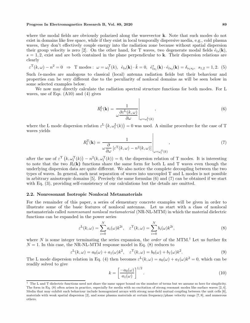
√ε law in local homogeneous and isotropic domains. Fig. 1

illustrates the T wave dispersion data in the two forms, the index of refraction function in Fig. 1(a),and the direct k = k(ω) function in Fig. 1(b). We study the T wave propagation characteristics withina given frequency band with center frequency ωc, which could serve as the carrier frequency in ananalog or digital communication system. The strength of spatial dispersion is varied according to thenormalized parameter ζ := −ω2

cb1/c2, with no spatial dispersion when ζ = 0. As can be seen from both

figures, as frequency increases, the propagation characteristics strongly deviates from the local antennascenario as ζ increases. In particular, the frequency-dependent index of refraction nT(ω) appears toasymptotically approach zero when spatial dispersion is very strong. This suggests that nonlocal Twave antennas may experience reduced radiation bandwidth under conditions of strong nonlocality, anobservation that will be confirmed by further results below.

To estimate the nonlocal antenna radiation pattern, we need to evaluate the fundamental Rl(k)function. Using Eq. (6) with the L mode dispersion relation in Eqs. (10) and (9), straightforward

(a) (b)

Figure 1. Dispersion analysis results for the nonresonant nonlocal metamaterial (NR-NL-MTM) whosemodel is given by (8) with case N = 1. We also further assume here negligible T wave response temporaldispersion (b0 = 1, ∂b1(ω)/∂ω = 0). (a) The transverse refraction index nT as function of frequency. (b)The transverse (T wave) mode dispersion relation. Here, ζ := −ω2

cb1/c2, where ωc := (ωmax − ωmin)/2

is the center frequency in the frequency band [ωmin, ωmax].


calculations give

RLl (k) =

1ω [a′0(ω) + a′1(ω)k2]

∣∣∣∣ω=ωL

l (k)

, (13)

where ωLl (k) can be obtained by inverting Eq. (10) and the prime indicates differentiation. For the T

modes, using Eq. (B1) in Eq. (7), the following expression is obtained for the T wave case:

RTl (k) =

1

ω∂

∂ωεT(k, ω) + 2n2(k, ω)

∣∣∣∣∣∣∣ω=ωT

l (k)

=1

2n(k, ω)∂

∂ω[ωn(k, ω)]

∣∣∣∣∣∣∣ω=ωT

l (k)

, (14)

where ωTl (k) is found by inverting Eq. (11). With the help of Eq. (9), expression (14) can be put into

the following general form

RTl (k) =

1

ωb′0(ω) + ωb′1(ω)k2 +2c2b0(ω)

c2 − ω2b1(ω)

∣∣∣∣∣∣∣∣ω=ωT

l (k)

. (15)

The expressions (13) and (15) can handle arbitrary temporal dispersion profiles for antennas radiatinginto isotropic nonlocal media of class N = 1 NR-NL-MTM. To gain further insight into the basicbehaviour of such antennas, we focus on the special but important case of negligible temporal dispersion.‡That is, for simplicity let us further assume that no temporal dispersion exists in the transverse dielectricresponse case, which is mathematically expressed by

b0(ω) = 1, b′1(ω) = 0. (16)

Therefore, the coefficients of the power series expansion in Eq. (8) are not dependent on frequency. Forthe special case of Eq. (16), the relation in Eq. (15) may be further reduced into

RT(k) =1

2n2T

∣∣∣∣ω=ωT(k)

=c2 − ω2

T(k)b1

2c2, (17)

where for simplicity we removed the modal index l since only one T wave exists for N = 1.§ In Sec. 3,the formula (17) will be exploited to explore various properties and characteristics of basic sourcesembedded into such class N = 1 NR-NL-MTM.

3. TRANSVERSE WAVE NONLOCAL ANTENNA SYSTEMS

We are ready now to tackle our first elementary radiating antenna system: the fundamental infinitesimaldipole antenna radiating at single frequency. This is nothing but a very short thin-wire antennaconcentrated at a position (say the origin) with orientation αs and frequency ωs. In spite of itsextreme simplicity, this source has received considerable attention in classical antenna theory, usuallyunder the rubric of Hertizan dipole [10], or electrically small antennas [11]. Moreover, it can beshown that any current that is not electrically small can be expanded into an optimized infinitesimaldipole model composed of only a few such infinitesimal sources [12–15]. For these reasons, we proposethat understanding the basic behaviour of a T wave nonlocal antenna should start with a thoroughinvestigation of such fundamental infinitesimal-dipole-based nonlocal antenna systems. Extension to Lwave type and arrays will be given in Secs. 4 and 5, respectively.

‡ Indeed, even though nonlocal metamaterials are expected to exhibit both spatial and temporal dispersion behaviour, in certainfrequency bands and wavenumber ranges, these two types of dispersion can be treated as independent phenomena [2, 3].§ It should be remembered that since b1 is negative, the ratio RT(k) is always positive and in fact less than one. Similarly, one canshow that RL(k) is between 0 and 1. Such inequalities follow from fairly general energy relations in dispersive electromagnetic mediaimposed by thermodynamic considerations and are valid also for anisotropic MTMs, e.g., see [3, 9].

92 Mikki

3.1. The Momentum Space Radiation Power Pattern of Continuous Sources

The expression of the infinitesimal dipole sinusoidal antenna current in spacetime is given by

Jant(r, t) = αsJsδ(r − rs)e−iωst, Jant(k, ω) = αseik·rs2πJsδ(ω − ωs), (18)

where rs is the location of the source and the frequency-dependent complex-valued quantity Js = Js(ωs)its strength. In order to utilize the radiation energy density expression [1]

Ul(k) =1ε0

Rl(k)∣∣∣k × Jant[k, ωl(k)]

∣∣∣2 , (19)

we evidently need to square a delta function because of Eq. (18). This can be achieved with the help ofthe generalized function identity [16, 17]

[2πδ(ω − ωs)]2 = T2πδ(ω − ωs), (20)

where T is the duration of the excitation, and the limit T → ∞ is implicit here. The spherical coordinatesform of k is given by

k = k(Ω) = x cos ϕ sin θ + y cos ϕ sin θ + z cos θ, (21)

where Ω := (θ, ϕ) and dk = dΩ. With the help of Eq. (20) after substituting Eq. (18) into Eq. (19),making use of Eqs. (17) and (21), we arrive at

PT(k, k) =c2 − ω2

T(k)b1

2c2ε0|(x cos ϕ sin θ + y cos ϕ sin θ + z cos θ)× αs|2 2π|Js|2δ(ωT,k − ωs), (22)

where the momentum-space power spectral density is defined by

Pl(k) := limT→∞

Ul(k)T

. (23)

The expression (22) gives the radiated power per unit momentum-space volume d3k/(2π)3 for transverse(T) waves emitted by a point source oriented along αs with source tuned to frequency ωs. The anglesθ and ϕ are those associated with observation in momentum space, hence their identification with k.For example, the total power radiated in the angular sector Ωr � k and within the wavenumber rangek1 < k < k2 is given by

Prad(k1 < k < k2, k ∈ Ωr) =∫ k2

k1

dk

∫Ωr

dΩ · PT(k, k). (24)

Physically, a radiation function of the form P (k, k) measures the radiated power density per unit solidangle per unit wavenumber, with units of Watt per solid angle per 1/m.

The wavenumber k can be considered a measure of the inverse of the characteristic wavelengthof the field’s spatial variation, so for small k the field possesses very large λ-components, while short-wavelength components correspond to k → ∞ [3, 4]. However, in controlled radiation theory, we rarelyenjoy fully freedom in regard to manipulating the production of the source’s wavelength components.Instead, what is typically available is the frequency of the externally-applied source/natural processpumping energy into the nonlocal material/metamaterial.

Now the key idea of this paper is that radiated energy can be computed in both momentum spaceand spacetime. Note that the delta function in Eq. (22) forces only one T mode to be excited, that inwhich k satisfies the condition ω(k) = ωs. This corresponds to the familiar condition in local radiationtheory where all emitted waves must satisfy k = ωs/c; however, due to the increased number andcomplexity of modes associated with radiation into nonlocal media, the antenna radiation pattern isexpected to be significantly altered qualitatively and quantitatively as will be discussed in Sec. 5.

Consequently, what is needed next is a general expression for the nonlocal antenna radiation patternexpressed as function of angles and frequency instead of angles and k, i.e., a function of the form Ul(ω, k)or Pl(k;ω) in line of the proposal given toward the end of Part I. We provide here a simple methodto derive such frequency-dependent radiation pattern valid for the case of generic isotropic nonlocal


domains. The most natural method is to equate energy in both representations, i.e., Ul(ω, k) is definedby the equality: ∫

d3k

(2π)3Ul(k) =

∫dω

∫dΩ Ul(ω, k). (25)

Note that in this paper we interchange k and Ω whenever convenient, see Eq. (21). To do so, thedispersion relation ωl(k) will be used, but in the more appropriate form

kl(ω) = kl(ω)k (26)

valid only if the index of refraction nl(ω, k) defined by Eq. (B1) is independent of k, which is the case inisotropic nonlocal media (The generalization to arbitrary media is given in Appendix B). The functionk = kl(ω) is obtained by inverting the dispersion relation ω = ωl(k). Note that by construction there isonly one mode captured by the dispersion relation ωl(k) so this function is injective (one-to-one), andhence invertible with one k-root for the equation ωl(k) − ω = 0, which we denote by kl.

Now, in spherical coordinates, the volume element in the momentum (spatio-spectral) space k maybe written as d3k = dkk2dΩ, while dk = (dkl/dω)dω. Therefore, the LHS of Eq. (25) can be expandedas ∫

d3k

(2π)3Ul(k) =

∫dωk2 dkl(ω)

dω

∫dΩUl[kl(ω), k]. (27)

Comparing Eq. (27) with Eq. (25), it is possible to deduce that

Ul(ω, k) =k2

l (ω)(2π)3

dkl(ω)dω

Ul[kl(ω), k]. (28)

Physically, the quantity in Eq. (28) represents the radiation energy density, or energy per unit solid angleper unit radian frequency (Watt per starad per rad/s). The total energy radiated within a frequencyband [ω1, ω2] and angular sector Ωr is given by

Urad(ω1 < ω < ω2, k ∈ Ωr) =∫ ω2

ω1

dω

∫Ωr

dΩ Ul(ω, k). (29)

On another hand, it is quite straightforward to compute the radiation pattern in terms of power insteadof energy. Using Eqs. (28) in (23), the observable radiation power pattern of the nonlocal point sourcecan be put in the form

PT(θ, ϕ;ω)=ω2

16π3ε0c2√

c2−ω2b1

|(x cos ϕ sin θ + y cos ϕ sin θ + z cos θ) × αs|2 2π|Js|2δ(ω − ωs), (30)

where ωs is the externally supplied (antenna) source frequency and the T wave dispersion relation inEq. (11) was utilized. The relation in Eq. (30) constitutes the T wave antenna (angular) radiationpower density (radiation pattern for short), i.e., the amount of power radiated by the T mode in thedirection (θ, ϕ) per unit frequency when a sinusoidal point source with frequency ωs and orientation αs

excites an isotropic nonresonant nonlocal metamaterial with N = 1. In particular, the total radiatedpower in the solid angular sector Ωr := {θ1 < θ < θ2, ϕ1 < ϕ < ϕ2} can be computed by means of theformula

Prad(Ωr) =∫ ∞

0dω

∫Ωr

dΩPT(θ, ϕ;ω) =∫ ∞

0dω

∫ θ2

θ1

∫ ϕ2

ϕ1

dθdϕ sin θ PT(θ, ϕ;ω). (31)

The proof of Eq. (31) follows directly from the manner in which Ul was constructed via relations of theform in Eq. (27).

94 Mikki

3.2. Antenna Directivity Analysis

Moving further, the sinusoidal radiator directivity is defined as the ratio of the maximum radiated powerdensity divided by the isotropic power density (the latter being the power density corresponding to idealisotropic radiator.) Quantitatively, this is given by [11]

D(ω) :=maxθ, ϕ P (θ, ϕ;ω)Prad(4π;ω)/2π

, (32)

where Prad(4π;ωs) is the radiated power on the entire infinite sphere. To give a concrete example, letus assume that the point antenna is located at the origin and oriented along the z-direction. In thiscase, |k × αs| = |k × z| = | sin θ|. From Eqs. (30) and (31), it follows that

Prad(4π;ω) =|Js|2ω2

8π2ε0c2√

c2 − ω2b1

∫ 2π

0dϕ

∫ π

0dθ sin3 θ =

|Js|2ω2

3πε0c2√

c2 − ω2b1

, (33)

where∫ π0 dθ sin3 θ = 4/3 was used. On the other hand,

maxθ, ϕ

PT(θ, ϕ;ω) =|Js|2ω2

8π2ε0c2√

c2 − ω2b1

maxθ, ϕ

| sin3 θ| =|Js|2ω2

8π2ε0c2√

c2 − ω2b1

. (34)

Therefore, from Eq. (32), the T wave nonlocal antenna has directivity DT = 1.5, which is the same asits value for local infinitesimal antennas. Therefore, sinusoidal T wave antennas of modes described bydispersion relation in Eq. (11) exhibit the same directive properties as conventional free-space antenna.‖

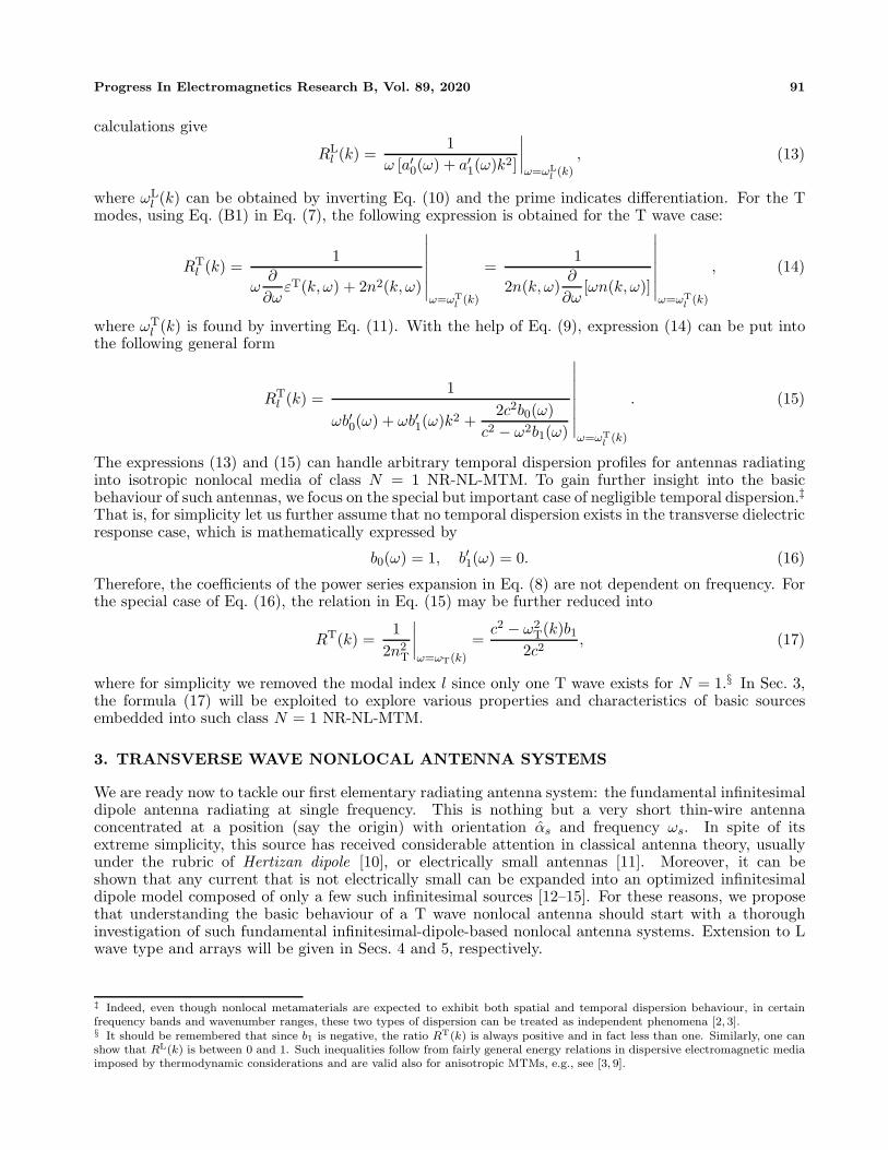
In Fig. 2, we illustrate one of those curious divergences in behaviour between local and nonlocalradiators. Fig. 2(a) shows the radiated total power (power radiated by all polarization components inall directions) computed by means of the expression (30) over a frequency band. The case with ζ = 0corresponds to zero spatial dispersion, i.e., local antennas (free-space radiators.) On the other hand, thecases ζ = 0.1, 0.5, 1, model class N = 1 non-resonant in isotropic metamaterials with increasing spatialdispersion strength, respectively. It is clear that the celebrated 1/λ2 power law in electromagnetictransmission is no longer satisfied at large frequencies in the case of this nonlocal T wave antennasystem. Indeed, the local antenna possesses a ω2 frequency law, while spatially dispersive media withthe T wave mode of the class N = 1 exhibits a linear ω frequency law or 1/λ variation for high frequency.This implies that electromagnetic waves radiated by this type of nonlocal T modes would experiencegreater decay of their high-frequency components, leading to smaller transmission bandwidth comparedwith local antennas. This striking behaviour can also be noticed in Fig. 2(b) where we plot the angularradiation pattern of a point source parallel to the z-direction, so θ measures the angle with the z-axis.It can be seen that with significant spatial dispersion (ζ = 1), the peak radiated power level of the Twave nonlocal antenna class N = 1 drops like 1/f with increasing frequency relative to the peak levelattained by the local antenna at the same frequency range.

3.3. Radiation Energy Patterns for Pulsed Signals

It is interesting to note that the theory developed in this paper is not exclusively restricted to sinusoidalsources of the form in Eq. (18). In fact, the momentum space approach is quite general and can handlearbitrary radiators in both space and time. To give a flavour of this possible expansion of the method,we stay within the relatively simple confines of the class N = 1 nonresonant nonlocal metamaterial wehave been exploring so far but now assume that the radiating source is excited by a rectangular pulserect(t/T ), where T is the total pulse duration.¶ The antenna current distribution in this case can be‖ Note, however, that this does not imply that directivity is the same in all other cases. The nonlocal antenna remains fundamentallydifferent from conventional free-space antennas in many respects. The first element among these distinctions is the existence of multiplemodes in nonlocal radiators, e.g., both T and L waves, which inherently changes the radiation pattern, leading to what was describedpreviously as “intrinsic material array effect” emerging from the fact that several modes may act like array antenna even though onlya single physical radiator exists [18–21]. Some of these directive emission differences marking nonlocal and local antenna systems areelaborated in general and for a few examples in Sec. 5.¶ See Fig. 3(b). Such pulses are essential in studying and designing modern digital communications. For example, digital datastreams can be modeled as a series of shifted rectangular pulses [22], see Fig. 3(a).


(a) (b)

Figure 2. T wave radiated power density pattern results for a sinusoidal radiator embedded into thenonresonant nonlocal metamaterial (NL-MTM) given by Eq. (8) with N = 1. We also further assumehere negligible temporal dispersion (b0 = 1, ∂b1(ω)/∂ω = 0). The normalized radiated power is definedas Prad/(3πε0c

3w2c )−1. (a) The radiated power as function of frequency computed using Eq. (30). Here,

ζ := −ω2cb1/c

2, where ωc := (ωmax −ωmin)/2 is the center frequency in the frequency band [ωmin, ωmax].(b) Total power radiated by a point source oriented along the z-direction. All results on the nonlocal(NL) antennas are computed for the case of ζ = 1. The local antenna (L) case is clearly ζ = 0, whileall other cases refer to nonlocal (NL) antennas (The L used in this figure should not be confused withlongitudinal waves used everywhere else in this paper.).

T2

T2

(a) (b)

Digital Data Stream rect(t/T)d(t)

T 3T t t

2T-

Figure 3. Rectangular pulses carry information in a digital communications link, e.g., (a) a digitaldata stream signal d(t). (b) A typical rectangular pulse is shown and is used to excite a point dipolesource embedded into a nonlocal metamaterials to explore the impact of such engineered domains onelectromagnetic radiation for potential deployment in wireless communications.

expressed in spacetime and momentum space via the relations

Jant(r, t) = αsJsδ(r − rs) rect(t/T ), Jant(k, ω) = αsJsT eik·rssinc(

ωT

2

), (35)

respectively, where αs, Js, and T are the source parameters and sinc(x) := sin (πx)/πx is the sincfunction. Substituting Eqs. (19), (35) and (17) into Eq. (28), the radiation energy density Ul(Ω;ω) canbe obtained, and after taking the limit in Eq. (23) we arrive at the momentum space radiation energydensity

UT(θ, ϕ;ω) =J2

s T 2ω2|sinc(ωT/2)|216π3ε0c2

√c2 − ω2b1

|(x cos ϕ sin θ + y cos ϕ sin θ + z cos θ)× αs|2 , (36)

where the dispersion relation in Eq. (11) was used. Similar to the calculation in Eq. (33), the totalenergy radiated by a dipole with rectangular pulse excitation can be obtained and is found to be given

96 Mikki

by

Urad(ω) =|Js|2T 2ω2|sinc(ωT/2)|2

6π2ε0c2√

c2 − ω2b1

. (37)

This is the positive (single-sided) power spectral density. To compute the net energy radiated by therectangular pulse, we integrate over all frequencies:

Erad = 2∫ ∞

0dωPrad(ω) =

∫ ∞

0dω

|Js|2T 2ω2|sinc(ωT/2)|23π2ε0c2

√c2 − ω2b1

. (38)

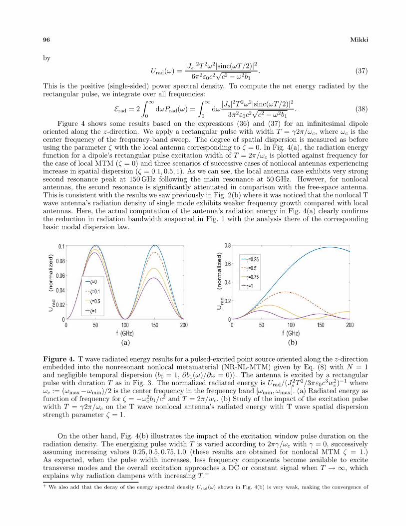
Figure 4 shows some results based on the expressions (36) and (37) for an infinitesimal dipoleoriented along the z-direction. We apply a rectangular pulse with width T = γ2π/ωc, where ωc is thecenter frequency of the frequency-band sweep. The degree of spatial dispersion is measured as beforeusing the parameter ζ with the local antenna corresponding to ζ = 0. In Fig. 4(a), the radiation energyfunction for a dipole’s rectangular pulse excitation width of T = 2π/ωc is plotted against frequency forthe case of local MTM (ζ = 0) and three scenarios of successive cases of nonlocal antennas experiencingincrease in spatial dispersion (ζ = 0.1, 0.5, 1). As we can see, the local antenna case exhibits very strongsecond resonance peak at 150 GHz following the main resonance at 50 GHz. However, for nonlocalantennas, the second resonance is significantly attenuated in comparison with the free-space antenna.This is consistent with the results we saw previously in Fig. 2(b) where it was noticed that the nonlocal Twave antenna’s radiation density of single mode exhibits weaker frequency growth compared with localantennas. Here, the actual computation of the antenna’s radiation energy in Fig. 4(a) clearly confirmsthe reduction in radiation bandwidth suspected in Fig. 1 with the analysis there of the correspondingbasic modal dispersion law.

(a) (b)

Figure 4. T wave radiated energy results for a pulsed-excited point source oriented along the z-directionembedded into the nonresonant nonlocal metamaterial (NR-NL-MTM) given by Eq. (8) with N = 1and negligible temporal dispersion (b0 = 1, ∂b1(ω)/∂ω = 0)). The antenna is excited by a rectangularpulse with duration T as in Fig. 3. The normalized radiated energy is Urad/(J2

s T 2/3πε0c3w2

c )−1 where

ωc := (ωmax−ωmin)/2 is the center frequency in the frequency band [ωmin, ωmax]. (a) Radiated energy asfunction of frequency for ζ = −ω2

cb1/c2 and T = 2π/wc. (b) Study of the impact of the excitation pulse

width T = γ2π/ωc on the T wave nonlocal antenna’s radiated energy with T wave spatial dispersionstrength parameter ζ = 1.

On the other hand, Fig. 4(b) illustrates the impact of the excitation window pulse duration on theradiation density. The energizing pulse width T is varied according to 2πγ/ωc with γ = 0, successivelyassuming increasing values 0.25, 0.5, 0.75, 1.0 (these results are obtained for nonlocal MTM ζ = 1.)As expected, when the pulse width increases, less frequency components become available to excitetransverse modes and the overall excitation approaches a DC or constant signal when T → ∞, whichexplains why radiation dampens with increasing T.+

+ We also add that the decay of the energy spectral density Urad(ω) shown in Fig. 4(b) is very weak, making the convergence of


4. LONGITUDINAL WAVE NONLOCAL ANTENNA SYSTEMS

Longitudinal (L) waves represent the second major type of electromagnetic waves excitable by sourcesembedded into nonlocal domains. The corresponding radiating systems will be dubbed L wave nonlocalantennas.� Our goal here is to investigate when such waves can be excited and how the combined Twave response developed in Sec. 3 and L wave radiation (to be developed shortly in this section) canbe joined together (the L-T array effect to be discussed in Sec. 5).

4.1. Some General Considerations for L Waves

Let us begin by first pointing out a peculiar fact about longitudinal waves. Since for L modes thewave is polarized along the direction of propagation, we have e∗l (k) = k, and therefore the L wavemomentum-space radiation energy density derived in Part I can be put in the form

Ul(k) =1ε0

Rl(k)|k · Jant[k, ωl(k)]|2. (39)

Writing the equation of continuity in the spatio-temporal domain then converting it to the momentumspace, we obtain, respectively

∂ρant(r, t)∂t

+ ∇ · Jant(r, t) = 0, k · Jant(k, ω) = ωρant(k, ω), (40)

where ρant is the electric charge density of electrical source corresponding to the externally appliedcurrent distribution Jant. Substituting Eq. (40) into Eq. (39), the following general form is obtained

Ul(k) =Rl(k)ω2

l (k)k2ε0

|ρant(k, ω)|2. (41)

The expression (41) is as good as the original form in Eq. (39). However, in certain applications, such asmicroscopic emission processes and certain applications in nanotechnology, it might be easier to expressthe radiating source as a charge density than as an antenna current distribution, and in the latter casethe relation in Eq. (41) is clearly more appropriate to work with. Nevertheless, in antenna applicationsand macroscopic electromagnetics, the formula (39) expressing radiation in terms of surface or volumecurrent distributions is preferred because the geometrical shape of the antenna can often be invoked torestrict the mathematical form of the current.�

One observation that immediately comes out after examining the L modes radiation formula whenexpressed in the alternative form Eq. (41) is that such waves can radiate only if the mode frequencyωl(k) is nonzero. While this might be expected, note that from the L mode dispersion relation inEq. (4) the dielectric function εL(k, ω) must depend on frequency. Otherwise, the equation εL(k, ω) = 0will not yield any specific value for ω for a given input k. This is clearer from the special case inEq. (10), where it is evident that no actual dispersion relation in the form ω = ωl(k) might obtainif the condition (∂/∂ω)εL = 0 is not satisfied. Therefore, the following conclusions is inevitable: Incontrast to T wave nonlocal radiators, effective L wave radiation would not be possible if the L dielectricfunction εL is independent of frequency ω. In other words, unlike T wave sources discussed in Sec. 3,temporal dispersion is fundamental in order to excite L waves in nonlocal domains. Therefore, in all thecoming calculations we will need to assume some concrete temporal dispersion model for the coefficientsai(ω) appearing in (8). However, it is important to remember that longitudinal and transverse responsefunctions are independent physical processes in general [2, 4].&

the total energy integral (38) slow. This is expected since the rectangular pulse excitation shown in Fig. 3 and implemented in thesource function in Eq. (35) assumes zero rise-/fall-times. In other words, this type of excitation current does not possess a first-orderderivative, which explains the slow decay of the energy spectral density. However, this represents no problem in principle for ourcomparative study with nonlocal radiators since both the local and nonlocal antennas are utilizing the same time pulse excitationform. In practice, we replace the ideal rectangular pulse by smooth pulses, e.g., Gaussian pulses [23], and those are known to haveFourier spectra with very rapid frequency decay, e.g., see [17].� In Sec. 2.2, the dispersion relation of L waves launched into isotropic media were derived, see the general Equation (4), and thespecial case of class N = 1 non-resonant type metamaterial in Eq. (10).� For example, in one dimensional antennas like wires or loops, the direction of current flow is fixed once and for all by the geometry.In cases like these and numerous others, the evaluation of the radiation energy density Ul(k) is expected to be considerably easierusing Eq. (39) than Eq. (41).& That is, while in some problems they may get entangled with each other, fundamentally speaking the dielectric functions εL and

98 Mikki

4.2. The Radiation Power Pattern of L Wave Antenna Systems

To evaluate the L wave radiation density function, it is to be noted first that the density expression (28)is still valid for L waves and hence when combined with Eq. (39) would give

UL(ω, k) =k2L(ω)

ε0(2π)3dkL(ω)

dωRL(ω)|k · Jant[kL(ω), k]|2 (42)

as the radiation energy pattern for the L wave antenna. Here, RL(ω) := R[kL(ω)].∧ Substituting the Lmode dispersion relation in Eq. (10) into Eq. (13) gives

RL(ω) =1

ω

[a′0(ω) + a′1(ω)

a0(ω)−a1(ω)

] =a1(ω)/ω

a′0(ω)a1(ω) − a′1(ω)a0(ω). (43)

Furthermore, from Eq. (6) we havedkL(ω)

dω=

12kL

ddω

[a0(ω)−a1(ω)

]=

−12kL

a′0(ω)a1(ω) − a′1(ω)a0(ω)a2

1(ω). (44)

Consequently, Eq. (42) evaluates to

UL(k;ω) =−nL(ω)

2ε0c(2π)3a1(ω)

∣∣∣k · Jant[kL(ω), k]∣∣∣2 , (45)

where the L wave index of refraction nL is given by

nL(ω) :=kL(ω)c

ω=

c

ω

√a0(ω)−a1(ω)

(46)

It is not possible to proceed further without specifying the functional forms of a0(ω) and a1(ω). Asstated earlier, these are some of the main MTM design parameters available for the material engineer.For maximum clarity and concreteness, let us assume that this design data is given by

a0(ω) = 1 − ω2p

ω2, −a1(ω) =

g2

ω2, (47)

which means that the host domain dielectric response function a0(ω) is assumed to follow the classicalDrude model with Plasma frequency ωp. The parameter g is assumed to be a positive real number.Its value, together with ωp, may be determined by the material’s physics and design. The dispersionrelation of the L wave in Eq. (10) now takes the form

k2L(ω) =

1g2

(ω2 − ω2

p

), ω2

L(k) = ω2p + g2k2. (48)

It is interesting to observe that the choice g =√

3Ve, where Ve is the thermal electron velocity in a hotplasma, results in the famous dispersion relation of Langmuir waves [2, 7]. Here, the thermal velocity isequal to

√kBTe/me, where Te and me are the temperature of the electron gas and the electron mass,

respectively, while kB is Boltzmann constant. While the underlying physical realization of nonlocalmetamaterials need not be restricted to plasma structures, we mention in passing that the Langmuir-type dispersion relations obtained with the choice g =

√3Ve are often considered accurate when the

phase velocity vp = ω/k is large compared with the thermal velocities of all species in the thermalplasma.� In general, the L mode index of refraction in Eq. (46) under the special case in Eq. (48)reduces into

nL(ω) =c

ωg

√ω2 − ω2

p =c

g

√1 − ω2

p

ω2=

c

ga0(ω). (49)

εT can be treated as two distinct functions. The material designer may then try to optimize the performance of some applications byindependently controlling the various internal parameters associated with each response function type, i.e., the array functions ai(ω)and bi(ω).∧ Note that we specify the L mode dispersion law by the subscript/superscript and suppress the modal index since the N = 1 classhas only one mode but the same formula is valid for other L modes in higher-order classes.� Usually ionic species are much slower than electrons due to the small electron/nucleus mass ratio provided the various ion gasestemperatures are not very large.


Note that for very large frequencies ω ωp, nL(ω) ∼ c/g, i.e., the index of refraction eventuallyconverges to constant level with increasing frequency, a behaviour very different from the T wave indexof refraction nT(ω) studied earlier, where in the latter case nT(ω) → 0 as ω → ∞ for the case of nonlocalmedia, see Fig. 2(a).

We many now proceed to compute the L wave antenna radiation pattern. Using Eqs. (47) and (49)in Eq. (45) leads to

UL(k;ω) =ω√

ω2 − ω2p

2ε0(2π)3g3

∣∣∣k · Jant[kL(ω), k]∣∣∣2 . (50)

This is the general L wave radiation formula in our special MTM case. For a sinusoidal antenna withradiating current in Eq. (18), the radiation power density can be obtained by a procedure identical tothe one employed to find Eq. (30). The result is

PL(θ, ϕ;ω) =ω√

ω2 − ω2p

16ε0π3g3|(x cos ϕ sin θ + y cos ϕ sin θ + z cos θ) · αs|2 2πJ2

s δ(ω − ωs). (51)

It is interesting to compare this form of the L mode radiation power density with the correspondingformula for T waves, i.e., Equation (30). Both seem to share several structural features, e.g., similar ω2

law for large frequencies. Also, since g has the unit of velocity, the appearance of factors containing g3 inthe denominator of the multiplicative fraction of (51) makes the latter very symmetrical in comparisonwith (30) where g is played there by c. In fact, when we consider the L-T combined response of nonlocalantenna systems in Secs. 5 and 6, it will be found that the ratio between these two characteristic L andT type speeds, namely g/c, will play a fundamental role.

Finally, we add another notable difference between T and L waves. It turns out that the momentumspace radiation function RL(k) has a fixed value

RL(k) =12

(52)

for L waves. On another hand, the corresponding relation for T waves in Eq. (17) is very different,exhibiting a strong function of k. Equation (52) can be proved by plugging the choice in Eq. (47) intoEq. (43) and performing some additional but straightforward manipulations which are omitted here forbrevity.

5. VIRTUAL ARRAYS IN NONLOCAL ANTENNA SYSTEMS

5.1. Principal Formulas

As will be shown below, it turns out that the key to understanding one of the most outstanding featuresof nonlocal antennas is the existence of multiple modes, transverse and longitudinal, that could beexcited simultaneously, leading to novel and unexpected radiation characteristics of external sourcesembedded into nonlocal domains. To see this, we continue working with the nonresonant nonlocalmetamaterial model given in Eq. (8). The L mode dispersion relation for arbitrary N is obtainedfrom (4) and it assumes the form

N∑i=0

ai(ω)k2i = 0, (53)

which is a polynomial equation in k2 of order N with frequency-dependent coefficients bi(ω). Note thatthese coefficients are real since by construction the dispersion relation is applied to the hermitian partof the response function [1]. However, even with real coefficients, the polynomial equation (53) haveN generally complex roots kL,l, l = 1, 2, ..., N. We are interested only in modes propagating away fromthe source carrying effective energy to the far zone, so roots with non-negligible imaginary part arediscarded and only those solutions of (53) consisting mainly of real wavenumber k are admitted. Let

100 Mikki

the number of these by NL ≤ N . Similarly, the T wave dispersion relation in Eq. (5) together withEq. (8) results in the following general polynomial equation in k

b0(ω) +[b1(ω) − c2

ω2

]k2 +

N∑i=2

bi(ω)k2i = 0, (54)

which is also an N -order polynomial equation in k2, leading to N generally complex roots kT,l,l = 1, 2, ..., N . Again, we only admit those roots with positive real part and negligibly small imaginarypart. Let us denoted their number by NT ≤ N. In sum, a total of NT +NL distinct L and T modes maybe excited by a nonlocal antenna compatible with a given source excitation frequency ω. Not all wavesmust be present at the same time and it is expected that a great care must be exhibited to ensure thatall modes are actually launched by the externally-introduced current Jant. In case this situation can beachieved, the total antenna radiation density pattern may be written in the following quite general form

U(ω, k) = UT(ω, k) + UL(ω, k), (55)

where

UT(ω, k) : =NT∑l=1

UTl (ω, k) =

NT∑l=1

k2T, l(ω)

ε0(2π)3dkT, l(ω)

dωRT, l(ω)|k × Jant[kT, l(ω), k]|2, (56)

UL(ω, k) : =NL∑l=1

ULl (ω, k) =

NL∑l=1

k2L, l(ω)

ε0(2π)3dkL, l(ω)

dωRL, l(ω)|k · Jant[kL, l(ω), k]|2. (57)

whereRT, l(ω) := RT

l [kT, l(ω)], RL, l(ω) := RLl [kL, l(ω)]. (58)

That is, the radiation pattern will consist of two major parts, one generated by all T modes and isgiven by UT(ω, k), while the L wave contribution is captured by the term UL(ω, k). The data needed tocompute the radiation pattern in its most general form are summarized in Table 1. It is to be observedthat the momentum-space radiation functions RL

l (k) and RTl (k) can be evaluated via Eqs. (6) and (7),

respectively, and that involves only knowledge of both the dielectric functions εL(ω, k) and εT(ω, k) andthe corresponding dispersion laws.

Table 1. Data needed to compute the radiation pattern of a generic antenna embedded into an isotropicnonlocal metamaterials with NT and NL T and L modes, respectively, radiating into the far zone.

Data Description

Jant(ω,k) Momentum-space source current distribution

k = kT, l(ω), l = 1, ..., NT NT dispersion functions for the T modes

k = kL, l(ω), l = 1, ..., NL NL dispersion functions for the L modes

εT(ω, k) T wave dielectric function

εL(ω, k) L wave dielectric function

� From the computational viewpoint, if the dispersion profiles of the modes are available, the only potential difficulty in computingthe total radiation pattern would stem from the need to estimate the derivatives dkl/dω for every mode. In addition, as can be seenfrom Eqs. (6) and (7), the calculations of RL

l (k) and RTl (k) themselves require estimating derivatives of the form ∂ε/∂ω. In this

paper, since all the examples given involve analytical approximation of the dispersion law, this does not present a problem. However,in future work, dispersion analysis of more complicated materials will involve working mainly with numerical data. In that case morecareful methods to estimate the group velocity dω/dk might be required since numerical differentiation is not a stable computationalmethod.


5.2. Virtual Arrays in with Single Sinusoidal Dipole Excitation

In order to better understand the key formulas (56) and (57), let us evaluate them for the special butfundamental case of a point source with sinusoidal excitation as described in Eq. (18). The relevantquantities in this case are the radiation power density obtained by means of Eq. (23) and are given by

PT(ω; θ, ϕ) =NT∑l=1

k2T, l(ω)RT, l(ω)

ε0(2π)3dkT, l(ω)

dω|(x cos ϕ sin θ + y cos ϕ sin θ + z cos θ)× αs|2 2πJ2

s δ(ω−ωs)

(59)for the radiation component mediated by T all excited transverse waves, while the correspondingcontribution due to longitudinal waves is collected in

PL(ω; θ, ϕ) =NL∑l=1

k2L, l(ω)RL, l(ω)

ε0(2π)3dkL, l(ω)

dω|(x cos ϕ sin θ + y cos ϕ sin θ + z cos θ) · αs|2 2πJ2

s δ(ω − ωs).

(60)We may now illustrate more directly the virtual array effect alluded to above, which is unique toradiation phenomena in nonlocal metamaterials. If one selects the orientation of the radiating dipole tocoincide with z, then the radiation spectral power densities in Eqs. (59) and (60) after integrating overall frequencies ω will result in

PTrad(ωs; θ, ϕ) =

J2s

4ε0π2

NT∑l=1

dkT, l(ω)dω

∣∣∣∣ω=ωs

k2T, l(ωs)RT, l(ω) sin2 θ, (61)

PLrad(ωs; θ, ϕ) =

J2s

4ε0π2

NL∑l=1

dkL, l(ω)dω

∣∣∣∣ω=ωs

k2L, l(ωs)RL, l(ω) cos2 θ. (62)

The expressions (61) and (62) provide radiation patterns complementary to each other. We first notethat for each T and L radiation law type, the angular pattern function, while possessing a temporalfrequency ω dependence, is essentially the same, namely that associated with the classic dipole sin2 θlaw in the case of T waves, and the cos2 θ for power law carried by L modes. On the other hand, if wecombine the T and L wave radiation patterns in Eqs. (61) and (62) according to Eq. (55), this wouldresult in different phenomena more akin to the array factor in conventional (local) antenna theory.Indeed, in this case the total radiated power pattern

Prad(ωs; θ, ϕ) = PTrad(ωs; θ, ϕ) + PL

rad(ωs; θ, ϕ) (63)can be put in the form

Prad(ω; θ, ϕ) =J2

s AL(ω)4ε0π2

[cos2 θ + A(ω) sin2 θ

], (64)

where

AL(ω) :=J2

s

4ε0π2

NL∑l=1

dkL, l(ω)dω

k2L, l(ω)RL, l(ω), AT(ω) :=

J2s

4ε0π2

NT∑l=1

dkT, l(ω)dω

k2T, l(ω)RT, l(ω), (65)

represent the L and T wave complex power pattern amplitudes, respectively, while their all-importantT-L power ratio is defined by

A(ω) :=AT(ω)AL(ω)

=

NT∑l=1

dkT, l(ω)dω

k2T, l(ω)RT, l(ω)

NL∑l=1

dkL, l(ω)dω

k2L, l(ω)RL, l(ω)

. (66)

� This, however, is valid for the present special case, and it depends on the radiation source, so the conclusion is not general enoughto cover arbitrary nonsinusoidal antennas.

102 Mikki

(a) (b)

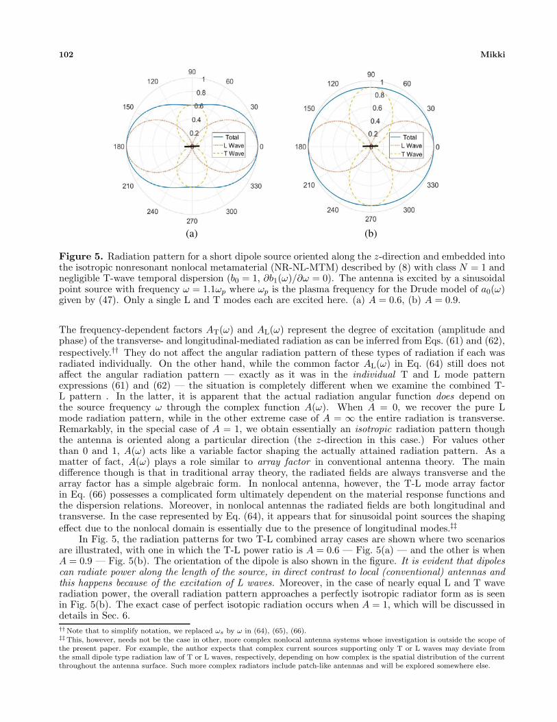
Figure 5. Radiation pattern for a short dipole source oriented along the z-direction and embedded intothe isotropic nonresonant nonlocal metamaterial (NR-NL-MTM) described by (8) with class N = 1 andnegligible T-wave temporal dispersion (b0 = 1, ∂b1(ω)/∂ω = 0). The antenna is excited by a sinusoidalpoint source with frequency ω = 1.1ωp where ωp is the plasma frequency for the Drude model of a0(ω)given by (47). Only a single L and T modes each are excited here. (a) A = 0.6, (b) A = 0.9.

The frequency-dependent factors AT(ω) and AL(ω) represent the degree of excitation (amplitude andphase) of the transverse- and longitudinal-mediated radiation as can be inferred from Eqs. (61) and (62),respectively.†† They do not affect the angular radiation pattern of these types of radiation if each wasradiated individually. On the other hand, while the common factor AL(ω) in Eq. (64) still does notaffect the angular radiation pattern — exactly as it was in the individual T and L mode patternexpressions (61) and (62) — the situation is completely different when we examine the combined T-L pattern . In the latter, it is apparent that the actual radiation angular function does depend onthe source frequency ω through the complex function A(ω). When A = 0, we recover the pure Lmode radiation pattern, while in the other extreme case of A = ∞ the entire radiation is transverse.Remarkably, in the special case of A = 1, we obtain essentially an isotropic radiation pattern thoughthe antenna is oriented along a particular direction (the z-direction in this case.) For values otherthan 0 and 1, A(ω) acts like a variable factor shaping the actually attained radiation pattern. As amatter of fact, A(ω) plays a role similar to array factor in conventional antenna theory. The maindifference though is that in traditional array theory, the radiated fields are always transverse and thearray factor has a simple algebraic form. In nonlocal antenna, however, the T-L mode array factorin Eq. (66) possesses a complicated form ultimately dependent on the material response functions andthe dispersion relations. Moreover, in nonlocal antennas the radiated fields are both longitudinal andtransverse. In the case represented by Eq. (64), it appears that for sinusoidal point sources the shapingeffect due to the nonlocal domain is essentially due to the presence of longitudinal modes.‡‡

In Fig. 5, the radiation patterns for two T-L combined array cases are shown where two scenariosare illustrated, with one in which the T-L power ratio is A = 0.6 — Fig. 5(a) — and the other is whenA = 0.9 — Fig. 5(b). The orientation of the dipole is also shown in the figure. It is evident that dipolescan radiate power along the length of the source, in direct contrast to local (conventional) antennas andthis happens because of the excitation of L waves. Moreover, in the case of nearly equal L and T waveradiation power, the overall radiation pattern approaches a perfectly isotropic radiator form as is seenin Fig. 5(b). The exact case of perfect isotopic radiation occurs when A = 1, which will be discussed indetails in Sec. 6.†† Note that to simplify notation, we replaced ωs by ω in (64), (65), (66).‡‡ This, however, needs not be the case in other, more complex nonlocal antenna systems whose investigation is outside the scope ofthe present paper. For example, the author expects that complex current sources supporting only T or L waves may deviate fromthe small dipole type radiation law of T or L waves, respectively, depending on how complex is the spatial distribution of the currentthroughout the antenna surface. Such more complex radiators include patch-like antennas and will be explored somewhere else.


5.3. Basic Examples

To illustrate the dependence on specific material parameters and frequency, we give a few basic examplesbased on the N = 1 class of isotropic nonresonant nonlocal metamaterial discussed above. From thedispersion relations of the T and L modes with NT = NL = 1, i.e., Equations (10) and (11), we readilycompute

AL(ω) =ω√

ω2 − ω2p

8π2ε0g3, AT(ω) =

ω2

8π2ε0c2√

c2 − ω2b1

, A(ω) =(g/c)3√

(1 − ω2b1/c2)(1 − ω2

p/ω2) . (67)

Figures 6(a) and 6(b) illustrate the variations of A(ω) with frequency for several degrees of nonlocalityin the T wave response as measured by the normalized parameter ζ. We first observe that as we changeζ from no transverse spatial dispersion (ζ = 0) to stronger transverse nonlocality characterized by largerpositive values, the change in the shape of the ratio of power divided between the T and L waves, i.e.,the array factor A(ω), is not very significant. In general, the overall trend observed is strong declinein the T-L power ratio as the operating frequency moves away from the plasma frequency ωp. Thisindicates that in this category of nonlocal antenna systems utilizing the N = 1-class NR-NL-MTM,power tends to concentrate in the longitudinal wave radiation component with all MTMs behaving as

limω→∞A(ω) =

{g3

c3 , b1 = 0,0, b1 = 0.

(68)

In other words, for this class of NR-NL-MTM, the cube of the velocity ratio g/c presents the minimumT-L power ratio at very large frequencies, providing a level at which the relative T and L waves’contribution to the total far-field radiation tend to stabilize. As we have seen before, g has the unitsof speed. If the NL-MTM is to be implemented using plasma domains, then g is likely to reflect thethermal velocity of the charged particles composing the plasma medium, e.g., electrons. In general, weprefer to keep the discussion at a more abstract and generic level in this paper where the goal is tounderstand the basic physics and design principles of nonlocal radiating systems. No concrete plasmamodel will be invoked in what follows, but we classify the range of possible values of the g-parameterto three distinctive cases: (i) Nonrelativistic regime (g c), (ii) superluminal�� regime (g > c), and(iii) relativistic regime (all remaining values of g). From Eq. (68), we can see that in the nonrelativisticregime, the T-L power ratio is small even when ζ is large (strong T wave response), implying that theL wave contribution to the far field will tend to dominate even when the T wave response is significant.Moreover, at higher frequencies the T-L ratio becomes even considerably smaller since (g/c)3 is muchless than g/c 1. This case is illustrated in Fig. 6(a). On the other hand, Fig. 6(b) shows that forlarger g/c, the T-L power ratio A becomes significantly larger at all frequencies. This suggests thatNL-MTMs designed to operate in the relativistic regime exhibit larger contribution of T waves to the farzone. Finally, in the superluminal regimes, calculations show that the T-L ratio could become greaterthan unity at all frequencies. For g → c but still g < c, A(ω) may become greater than unity in thelower edge of the frequency range ω > ωp.

5.4. Virtual Arrays and Antenna Directivity

Finally, let us estimate the directivity of the nonlocal antenna system exhibiting virtual array effectsby focusing on the radiation power pattern in Eq. (64) with the data in Eq. (67). From the definitionof directivity formula (32), we have

D(ω) :=maxθ,ϕ Prad(θ,ϕ;ω)

Prad(4π;ω)/4π= 4π

maxθ,ϕ


]∫ 2π

0dϕ

∫ π

0dθ sin θ


] . (69)

�� The term ‘superluminal’ does not imply a violation of special relativity since all relevant velocities are phase velocities or ω/k,which can be greater than speed of light. Group velocity is usually bounded by the speed of light if expresses energy transportvelocity.

104 Mikki

(a) (b)

Figure 6. Virtual array effects in the radiation by a point source oriented along the z-directionembedded into class N = 1 isotropic nonresonant nonlocal metamaterial (NR-NL-MTM) given by (8)and negligible T wave temporal dispersion (b0 = 1, ∂b1(ω)/∂ω = 0)). The antenna is excited bya sinusoidal point source with frequency ω while ωp is the plasma frequency for the Drude modela0 = 1 − ω2

p/ω2 and a1 = −g2/ω2. (a) Variation of A(ω) with frequency for g/c = 0.1. (b) Variation of

A(ω) with frequency for g/c = 0.5.

Using∫ π0 dθ sin3 θ = 4/3 and

∫ π0 dθ sin θ cos2 θ = 2/3, this evaluates into

D(ω) =maxθ, ϕ

{1 + [A(ω) − 1] sin2 θ

}1/3 + 2/3A(ω)

=

⎧⎪⎪⎨⎪⎪⎩

3A(ω)1 + 2A(ω)

, A(ω) ≥ 1,

6 − 3A(ω)1 + 2A(ω)

, A(ω) < 1.(70)

Evidently, this is very different from the classic dipole directivity of D = 3/2. In fact, the later isobtained only when A → ∞ since this is the case when AL = 0, i.e., the L wave does not exist. On theother hand, the maximum directivity that can be attained by this system is D = 6 and occurs whenA = 0, i.e., when the entire radiation is due to L waves. For other intermediate case, the directivitycan assume the range of values depicted in Fig. 7. In the range 0 ≤ A < 1, L waves dominate thecomposition of the radiated fields, while at A = 1 the critical transition from L-mode-dominated toT-mode-dominated composition occurs. As A increases, the radiation field tends to become essentiallytransverse. Therefore, use of carefully-designed nonlocal MTMs may lead to significant increase inthe directivity of an infinitesimal dipole antenna from 1.5 to 6, i.e., four times the classical antennadirectivity.

6. ENGINEERING APPLICATION: SHAPING THE RADIATION PATTERN TOPRODUCE ISOTROPIC ANTENNA SYSTEMS

6.1. Exact Design Equations

A quick application is developed here where the main idea is to theoretically demonstrate how thedesign of a suitable nonlocal MTM may lead to the construction of future radiating system exhibitingisotropic radiation pattern. For simplicity, we continue to focus on the special but fundamental case ofinfinitesimal dipole source with time-harmonic excitation. The nonlocal T-L array factor in Eq. (66)can be put in the form

A(ω) = F[ω, εT(k, ω), εL(k, ω), NT, NL

](71)

in order to emphasize the design parameters available to the engineer, where F is the generic functionalform of the dependence on such parameters. The data that must be found to design the system are


Figure 7. Directiviy of a nonlocal antenna system with single T and L modes vs. the T/L power ratioA.

encoded in the T and L dielectric response functions εT(k, ω), εL(k, ω). These in turns determine thedispersion law data kT(ω), kL(ω). The numbers of T and L modes NT, NL must also be determined bythe designer. If the desired radiation pattern is required to be isotropic, then from Eq. (64) we easilydeduce that a sufficient condition for this to happen is given by the equation A(ω) = 1, or in details

NT∑l=1

dkT, l(ω)dω

k2T, l(ω)RT, l(ω) =

NL∑l=1

dkL, l(ω)dω

k2L, l(ω)RL,l(ω). (72)

From the form of Eq. (71), the unknowns to be estimated in this case are εT(k, ω), εL(k, ω) for a givenfrequency ω and numbers of modes NT, NL. The relation in Eq. (72) is the general design equation forsinusoidal isotropic nonlocal antenna systems utilizing an isotropic metamaterial.

We give an example illustrating the design process by specializing for the class N = 1 NR-NL-MTM.Making use of Eq. (65), the isotropic radiator design equation (72) reduces to

g = c

[(1 − ω2b1

c2

)(1 − ω2

p

ω2

)]1/6

. (73)

The relation in Eq. (73) represents the main design equation for isotropic nonlocal antenna systemsusing class N = 1 NL-MTM. It spells out the exact connection between this MTM’s design parametersb1 and g on one hand, and the operating frequency on another. Design curves are given in Fig. 8(a)and Fig. 8(b). In Fig. 8(a), the velocity ratio g/c is plotted across frequency for several possible valuesof ζ, allowing us to assess the impact of the T wave’s degree of nonlocality — as measured by ζ — onthe ability to attain perfectly isotropic radiators. The results suggest that for local T wave response(ζ = 0), the optimum value of g approaches the speed of light c as the antenna frequency increasessufficiently away from the plasma frequency ωp since in such scenario we inherently enter the relativisticregime. Hence, to properly design a plasma-type NL-MTM for this application, one needs to operate asclose to ωp as possible if it is desired to remain within the nonrelativistic regime. However, as we startto inject nonlocal behaviour into the MTM by gradually increasing ζ, the optimum value of g shiftsinto the relativistic regime at much lower frequencies compared with the local T wave case (ζ = 0). Infact, at sufficiently large values for ζ, the optimum g-parameter value enters the superluminal regimeat operating frequencies fairly close to ωp. This general behaviour is further investigated in Fig. 8(b)where we focus on how the optimum value of g changes with the T wave’s nonlocality parameter ζ atspecific frequency. We there find that whenever the operating frequency is shifted away from ωp, theNL-MTM design parameters enter the relativistic then the superluminal regimes with even increasingζ. This behaviour becomes more acute at higher frequencies. For example, in the case of ω = 1.5ωp, the

106 Mikki

(a) (b)

Figure 8. Design curves for perfectly isotropic power radiation by a point source oriented along thez-direction embedded into class N = 1 isotropic nonresonant nonlocal metamaterial (NR-NL-MTM)given in (8) and negligible T wave temporal dispersion (b0 = 1, ∂b1(ω)/∂ω = 0)). The antenna isexcited by the sinusoidal point source with frequency ω while ωp is the plasma frequency for the Drudemodel a0 = 1 − ω2

p/ω2 and a1 = −g2/ω2. We use (73) to estimate the optimum design value of g in

two cases: (a) Variation of optimum isotropic g with frequency for various values of ζ := −ω2pb1/c

2. (b)Variation of optimum isotropic g with ζ for various frequencies.

NL-MTM becomes superluminal starting from just around ζ = 0.4. The overall conclusion here is thatone would expect the MTM to exhibit weaker T-wave-type nonlocality in order to realize the optimumL wave design parameter g if the latter is to be associated with particle velocities much lower than c.§§

6.2. Alternative Design Procedure Based on Optimization

There are two potential difficulties with the exact design equation (72). First, it is not immediatelyclear that for a given frequency and number of modes that relation can yield useful solution forεT(k, ω), εL(k, ω). Even if such solutions exist, the realization of the nonlocal metamaterial mightbe not available for the range of values obtained. Second, the design approach encapsulated by Eq. (72)is inherently a single-frequency approach and hence inherently narrowband. For many applications,especially modern wireless communication system, the bandwidth could be much larger. To resolvethese two difficulties, an approximation is more suited. The idea is that instead of enforcing an exactisotropic radiator, one may construct a suitable cost function to measure the deviation of the actuallyobtained radiation pattern from a target isotropic reference

Pref(ω; θ, ϕ) :=J2

s AL(ω)4ε0π2

. (74)

One such suitable cost measure can be the minimum mean square error (MMSE) function

C[εT(k, ω), εL(k, ω), NT, NL

]:=

1ωmax − ωmin

∫ ωmax

ωmin

dω1Ωr

∫Ωr

dΩ|Prad(ω; θ, ϕ) − Pref(ω; θ, ϕ)|2, (75)

where a convenient numerical optimization of this error will be performed over both the frequencyinterval of interest [ωmin, ωmax] and the radiation pattern observed over a given solid angle sector Ωr.The goal then is clearly to use powerful optimization algorithm to numerically search for the bestnonlocal metamaterial parameters εT(k, ω), εL(k, ω), NT, NL, such that the error C is minimum. This is§§ However, note that relativistic corrections on speed in plasma have been known long time ago, e.g., see the analysis of the so-calledrelativistic plasma [2, 4, 8]. Also, radiation phenomena in which the radiating particles are relativistic (Cherenkov radiation) are wellunderstood [4, 24]. Finally, we add that the generic nonresonant nonlocal metamaterial discussed here need not be exclusively realizedas hot plasma domain; other technologies might be deployed in the future to implement such metamaterial system such as near-fieldcoupled dense packing domains, metasurfaces, or other periodic structures.


usually attained with additional constraints on the available ranges for these optimization parameterscaused by material availability, leading effectively to constrained optimization problems. In this way, anonlocal metamaterial may be designed to realize a wideband isotropic nonlocal antenna system.

7. CONCLUSION

We provided a detailed application of the general momentum-space radiation theory expounded inPart I focusing on the special but essential case of nonlocal isotropic metamaterials. The specializeddispersion and radiation formulas corresponding to this scenario were derived in details and severalanalytical and numerical examples were provided to illustrate the use of the theory in describing anddesigning nonlocal antenna systems. In particular, we studied the behaviour of transverse (T) andlongitudinal (L) wave antennas and explored some of their properties. Comparison with local antennacounterparts were given for the cases of time-harmonic and rectangular pulse excitation of infinitesimaldipole sources. Bandwidth and directivity performance were investigated and the distinctive differencesbetween local and nonlocal antennas were explicated. As a more striking difference we also exploredvirtual array phenomena in nonlocal domains and showed that single sources can have array-factor likeradiation pattern. One of the possible engineering applications demonstrated here was the design ofperfectly isotropic antenna systems using small dipoles launching a proper combination of T and Lwaves. Also, we computed the directivity of a combined L-T system and predicted that it may reachfour times the value of classical (local) antenna under certain (design) conditions.

APPENDIX A. ISOTROPIC SPATIALLY-DISPERSIVE TENSOR FORMULAS ANDSOME OF THEIR PROPERTIES

We work with a medium possessing a dielectric tensor given by Eq. (1). In this case, we can write

G−1, L(k, ω) = εL(k, ω)kk, G−1, T(k, ω) =(εT(k, ω) − n2

)(I − kk), (A1)

where the momentum-space dyadic GF

G−1(k, ω) := −k2c2

ω2

(I − kk

)+ ε(k, ω) (A2)

from [1] and n2 = k2c2

ω2 were used. From the definition of matrix determinant, we conclude

G−1,L(k, ω) = εL(k, ω), G−1,T(k, ω) = εT(k, ω) − n2. (A3)

It can also be shown by direct calculations that the following decomposition hold

G−1(k, ω) = εL(k, ω)[εT(k, ω) − n2

]2. (A4)

On the other hand, expanding the co-factor matrix into longitudinal and transverse parts, we arrive at

C(k, ω) =(εT(k, ω) − n2

) [(εT(k, ω) − n2

)kk + εL(k, ω)(I − kk)

]. (A5)

In particular, the forward Green’s function of this special nonlocal medium acquires the simple form

G(k, ω) =

(εT(k, ω) − n2

)kk + εL(k, ω)(I − kk)

εL(k, ω) (εT(k, ω) − n2). (A6)

Let us now evaluate the trace of the co-factor matrix. Noting the relations tr[kk] = 1, tr[I] = 3, thetrace function γl(k) := tr[C(k, ωl(k))] from [1] applied to Eq. (A5) yields

γl(k) :=(εT(k, ω) − n2

) [(εT(k, ω) − n2

)+ 2εL(k, ω)

]. (A7)

Next, in order to estimate the crucial Rl(k) function

Rl(k) =γl(k)

ω∂G−1(k, ω)/∂ω

∣∣∣∣ω=ωl(k)

(A8)

108 Mikki

constructed in [1], we use Eq. (A4) to compute

∂G−1(k, ω)∂ω

=∂εL(k, ω)

∂ω

[εT(k, ω) − n2

]2+ 2εL(k, ω)

(εT(k, ω) − n2

) ∂(εT(k, ω) − n2

)∂ω

, (A9)

which after substituting into Eq. (A8) and making use of Eq. (A7) results in the following expression

Rl(k) :=

(εT(k, ω) − n2

)+ 2εL(k, ω)

ω∂εL(k, ω)

∂ω(εT(k, ω) − n2) + 2ωεL(k, ω)

∂(εT(k, ω) − n2

)∂ω

∣∣∣∣∣∣∣∣ω=ωl(k)

(A10)

valid for arbitrary nonlocal isotropic and optically inactive metamaterials. Even though Eq. (A10)may still look complicated, it has the advantage that it does not require evaluating the modal fielddistribution functions el(k) and depends only on the dispersion relations ωl(k) and the material tensorfunctions.

APPENDIX B. THE MOMENTUM-SPACE RADIATION FORMULA FOR GENERICTIME-DOMAIN SOURCES

We convert the radiation formula (2) into a form more convenient for antenna applications involvingarbitrary nonlocal metamaterial domains, i.e., not restricted to the isotropic media of Sec. 3. Thedirection of wave propagation is k := k/k, so we may describe this direction by a solid angle Ω. Themagnitude k = |k| is related to frequency through the mode dispersion relation ω = ωl(k, k). It isbetter, however, to express the dispersion relation in the form

k2c2

ω2= n2

l

(ω, k

), (B1)

which is very frequently used in optics [5]. Here, nl is the index of refraction of the lth mode and thepositive square root of Eq. (B1) is assumed. The volume element d3k/(2π)3 in momentum space cannow be re-expressed in spherical coordinates, then we transform k to ω using Eq. (B1). Therefore,

∫R3

d3k

(2π)3=∫ ∞

0dω

∫4π

dkω2n2

l

(ω, k

)(2πc)3

∂

∂ω

[ωnl

(ω, k

)]. (B2)

We now introduce the antenna radiation pattern Ul(ω, k), which is defined by∫R3

d3k

(2π)3Ul(k) =

∫ ∞

0dω

∫4π

dk Ul

(k, k)

. (B3)

Physically, Ul(ω, k) is the energy radiated in standard time interval with duration T per unit frequencyper unit solid angle. Using Eqs. (B2) and (2), we finally arrive at

Ul

(ω, k

)=

ω2n2l

(ω, k

)(2πc)3

∂

∂ω

[ωnl

(ω, k

)]Ul

[(ω/c)nl

(ω, k

)k], (B4)

whereUl

[(ω/c)nl

(ω, k

)k]

= J∗ant(k, ω) · Rl(k) · Jant(k, ω)

∣∣k=(ω/c)nl(ω, k)k . (B5)

In writing Eqs. (B4) and (B5), we have used k = kk then re-expressed k in terms of ω and k with thehelp of Eq. (B1). Consequently, the radiation mode antenna pattern intensity as function of directionand frequency is completely determined by the dispersion relation in Eq. (B1).


REFERENCES

1. Mikki, S., “Theory of electromagnetic radiation in nonlocal metamaterials: A momentum spaceapproach — Part I (submitted),” Progress In Electromagnetics Research B, Vol. 89, 63–86, 2020.

2. Ginzburg, V. L., The Propagation of Electromagnetic Waves in Plasmas, Pergamon Press, Oxford,New York, 1970.

3. Landau, L. D., Electrodynamics of Continuous Media, Butterworth-Heinemann, Oxford, England,1984.

4. Ginzburg, V. L., Theoretical Physics and Astrophysics, Pergamon Press, Oxford, New York, 1979.5. Agranovich, V. and V. Ginzburg, Crystal Optics with Spatial Dispersion, and Excitons, Springer

Berlin Heidelberg Imprint Springer, Berlin, Heidelberg, 1984.6. Halevi, P., Spatial Dispersion in Solids and Plasmas, North-Holland, Amsterdam, New York, 1992.7. Ilinskii, Y. A. and L. Keldysh, Electromagnetic Response of Material Media, Springer

Science+Business Media, New York, 1994.8. Sitenko, A. G., Electromagnetic Fluctuations in Plasma, Academic Press, 1967.9. Fabrizio, M. and A. Morro, Electromagnetism of Continuous Media: Mathematical Modelling and

Applications, Oxford University Press, Oxford, 2003.10. Schelkunoff, S. A. and H. T. Friss, Antennas: Theory and Practice, Chapman & Hall, London,

New York, 1952.11. Balanis, C. A., Antenna Theory: Analysis and Design, 4th Edition, Inter-Science, Wiley, 2015.12. Mikki, S. and A. Kishk, “Theory and applications of infinitesimal dipole models for computational

electromagnetics,” IEEE Transactions on Antennas and Propagation, Vol. 55, No. 5, 1325–1337,May 2007.

13. Mikki, S. and Y. Antar, “Near-field analysis of electromagnetic interactions in antenna arraysthrough equivalent dipole models,” IEEE Transactions on Antennas and Propagation, Vol. 60,No. 3, 1381–1389, March 2012.

14. Clauzier, S., S. Mikki, and Y. Antar, “Generalized methodology for antenna design through optimalinfinitesimal dipole model,” 2015 International Conference on Electromagnetics in AdvancedApplications (ICEAA), 1264–1267, September 2015.

15. Mikki, S. and Y. Antar, “On the fundamental relationship between the transmitting and receivingmodes of general antenna systems: A new approach,” IEEE Antennas and Wireless PropagationLetters, Vol. 11, 232–235, 2012.

16. Zeidler, E., Quantum Field Theory II: Quantum Electrodynamics, Springer, 2006.17. Godement, R., Analysis II: Differential and Integral Calculus, Fourier Series, Holomorphic

Functions, Springer-Verlag, Berlin, 2005.18. Mikki, S. M. and A. A. Kishk, “Electromagnetic wave propagation in nonlocal media: Negative

group velocity and beyond,” Progress In Electromagnetics Research B, Vol. 14, 149–174, 2009.19. Mikki, S. and Y. Antar, “On electromagnetic radiation in nonlocal environments: Steps toward

a theory of near field engineering,” 2015 9th European Conference on Antennas and Propagation(EuCAP), 1–5, April 2015.

20. Mikki, S. and Y. Antar, New Foundations for Applied Electromagnetics: The Spatial Structure ofFields, Artech House, London, 2016.

21. Mikki, S., “Exact derivation of the radiation law of antennas embedded into generic nonlocalmetamaterials: A momentum-space approach,” 2020 14th European Conference on Antennas andPropagation (EuCAP), 1–5, 2020.

22. Lathi, B. P. and Z. Ding, Modern Digital and Analog Communication Systems, Oxford UniversityPress, New York, 2019.

23. Sarkar, D., S. Mikki, K. V. Srivastava, and Y. Antar, “Dynamics of antenna reactive energy usingtime-domain IDM method,” IEEE Transactions on Antennas and Propagation, Vol. 67, No. 2,1084–1093, Feb. 2019.

24. Schwinger, J., et al., Classical Electrodynamics, Perseus Books, Mass, 1998.

progress in electromagnetics research

Documents