aneffectivetechniqueforreducingthe … · progress in electromagnetics research, pier 73,...

Progress In Electromagnetics Research, PIER 73, 213–238, 2007

AN EFFECTIVE TECHNIQUE FOR REDUCING THETRUNCATION ERROR IN THENEAR-FIELD-FAR-FIELD TRANSFORMATION WITHPLANE-POLAR SCANNING

F. D’Agostino, F. Ferrara, C. Gennarelli, R. Guerrieroand G. Riccio

Dipartimento di Ingegneria dell’Informazione ed Ingegneria ElettricaUniversity of SalernoVia Ponte Don Melillo, 84084 Fisciano (Salerno), Italy

Abstract—An effective approach is proposed in this paper forestimating the near-field data external to the measurement region inthe plane-polar scanning. It relies on the nonredundant samplingrepresentations of the electromagnetic field and makes use of thesingular value decomposition method for the extrapolation of theoutside samples. It is so possible to reduce in a significant way the errordue to the truncation of the measurement zone thus increasing the far-field angular region of good reconstruction. The comparison of suchan approach, based on the optimal sampling interpolation expansions,with an existing procedure using the cardinal series has highlightedthat the proposed technique works better. Some numerical tests arereported for demonstrating its effectiveness.

1. INTRODUCTION

The nonredundant sampling representations of electromagnetic (EM)fields [1], which are based on the spatial bandlimitation properties [2]of the fields radiated by finite size sources, allow a very remarkablereduction of the near-field (NF) data to be acquired in the case ofelectrically large antennas and extended scanning regions. As a matterof fact, the NF data required to perform the near-field-far-field (NF-FF) transformations are recovered from the collected ones by usingproper sampling interpolation formulas [3–10].

When the measurement region is truncated, such as in thecylindrical and planar scannings, an inevitable truncation error affectsthe NF data reconstruction in the zones close to the boundary of such

214 D’Agostino et al.

a region. As a consequence, the reconstruction results to be accuratein a zone smaller than the measurement one (since the required guardsamples must belong to this last) and this implies a reduction of theangular region wherein an accurate FF reconstruction is attained. Ofcourse, an enlargement of this last region can be obtained by decreasingthe distance between the antenna under test (AUT) and the scanningsurface. However, such a distance cannot be reduced beyond certainlimits, otherwise the interactions between the AUT and the probecannot be neglected any more.

An extension of the zone of “good NF reconstruction” is achievableby employing the optimal sampling interpolation (OSI) expansionsinstead of the cardinal series (CS) ones. In fact, when evaluating thefield (or the voltage measured by the probe) at each needed point, theselast require the use of many samples to keep the truncation error lowand this leads to a large computational time too. On the contrary, theOSI expansions minimize the truncation error for a given number ofretained samples and, therefore, they require only a reduced number ofdata in the neighbourhood of the output point. Furthermore, the useof OSI expansions allows one to overcome the other serious drawbackof the CS ones, i.e., the propagation of the errors affecting the datafrom high to low field (voltage) regions [11], due to the slow decay ofthe interpolation functions.

It is worth noting that, although the use of the nonredundantsampling representations of the EM field is extremely convenient fromthe data reduction viewpoint, it gives rise to an unavoidable decreasein the ratio between the extensions of the accurate reconstruction zoneand the measurement one. In fact, in such a case the guard samplesrepresent a more relevant percentage of the overall number of data andlie in the peripheral zones, where the sample spacing is remarkablygreater than in the central region. Accordingly, in order to obtainan accurate field (voltage) reconstruction in the whole measurementregion, it becomes very important to estimate a proper number ofoutside samples.

In light of the above discussion, we are led to the followingextrapolation problem: estimation of a (spatially) bandlimitedfunction outside the observation region from the knowledge of itsinternal samples taken at a rate greater than the Nyquist one. Aswell-known, this is an ill-posed problem widely studied in literaturewith reference to the case of bandlimited signals which are known onlyin a finite time interval [12–21].

It is well-known that a continuous bandlimited signal can beextrapolated, without error, outside any finite interval. To this end,a Taylor series expansion can be used, since such a signal is analytic.

Progress In Electromagnetics Research, PIER 73, 2007 215

In practice, such a procedure is not feasible, because observed dataare always corrupted by noise and the evaluation of derivatives isa noise-sensitive process. A different procedure using the prolatespheroidal wave functions has been proposed by Slepian and Pollakin [12]. Unfortunately, also this method is sensitive to the errorsaffecting the data and is onerous from the computational viewpoint.Papoulis introduced in [13] an iterative algorithm, which reduces ateach iteration the mean-square error between the estimated and theoriginal (time unbounded) signal. He compared it with that using theprolate spheroidal wave functions and showed that his method worksbetter.

When considering discrete signals, the analyticity propertyvanishes, due to their sampling representation. Therefore, otherconstraints besides the limited bandwidth assumption are requiredin order to achieve an accurate solution. A discrete version of theiterative algorithm proposed by Papoulis has been developed in [14].Moreover, in the same paper, a noniterative method has been proposedfor solving the extrapolation problem from noise-free observations bymeans of an extrapolation matrix. In [15], Cadzow proposed a differentextrapolation matrix, which does not have the existence problem ofthat suggested in [14]. In both papers, the solutions for the discretecase have been obtained by sampling the continuous solutions. Thecriterion of the minimum norm least squares for the extrapolationof the signal from observations containing additive noise has beenintroduced by Jain and Ranganath in [16]. In any case, as explicitlystated in [17], extrapolation techniques in presence of noise mustbe used judiciously in order to obtain reasonable results. Since theextrapolation can be viewed as a minimum norm least squares solutionof a generally ill-posed system of linear equations, Sullivan and Liusuggested the use of the singular value decomposition (SVD) methodfor controlling the ill-conditioning [18]. A regularization procedure,based on the SVD and employing multiple regularization parametersto be determined optimally, has been proposed in [19] to deal withdata affected by white Gaussian noise. Other considerations on thestability of the estimation procedure can be found in [20].

As explicitly stated in [21], when the samples are error affected, anaccurate extrapolation of the signal is possible for at most a boundeddistance beyond the observation interval. Accordingly, since physicalmeasurements can never be perfect, this implies that only few samplesexternal to the observation interval can be reliably estimated. This lastconsideration justifies why the extrapolation techniques have scarcelyattracted the attention of the antenna measurement community. Infact, until the standard and redundant sampling representations (based


on the truncation of the spectrum to the visible region and, then, usinga sample spacing at most equal to λ/2, λ being the wavelength) werethe only available ones, the estimation of few external samples wouldhave allowed a very limited extension of the zone wherein the near fieldwas known.

The development of nonredundant sampling representations ofEM fields has deeply modified the scenario [22]. In fact, by using theselast representations, the sample spacing, as already stated, increasesremarkably when moving far away from the center of the scanningregion. Accordingly, even the estimation of very few samples externalto such a region allows a noticeable extension of the zone wherein thenear field is known, thus enlarging in a significant way the angularregion wherein an accurate FF reconstruction is attained. In thisframework, an approach for reducing the truncation error in the NF-FFtransformations with plane-polar and cylindrical scannings has beendeveloped in [22, 23] and [24], respectively. Such an approach is basedon the aforementioned nonredundant representations and makes use ofthe CS expansions and of the SVD method for recovering the outsidedata.

A convenient OSI based extrapolation procedure for estimatingthe outside samples on a NF line is described in the following Sectionand compared with the technique using the CS expansions. Such anapproach is properly extended in Section 3 to the extrapolation ofthe NF data external to the measurement region in the plane-polarscanning. At last, conclusions are collected in Section 4.

2. NF EXTRAPOLATION ALONG A LINE

In this Section the OSI expansions based extrapolation techniquefor recovering the samples external to the measurement region alonga straight line in the NF region of an electrically large antenna isdescribed and compared with that employing the CS expansions. Quiteanalogous results can be obtained when considering a two-dimensionalobservation domain too.

Without any loss of generality, let us consider an AUT enclosedin an oblate ellipsoidal surface Σ (having major and minor semi-axesequal to a and b) and a radial line of a plane-polar domain at distanced in the NF region (see Fig. 1).

According to [1], a nonredundant sampling representation can beobtained by introducing the “reduced electric field”

F (ξ) = E(ξ)ejγ(ξ) (1)

wherein the phase factor γ to be singled out from the field expression


y

d

x 2a

2b

P( k)z

P( n)

max

Figure 1. Relevant to a rectilinear observation domain. Dots: regularsamples. Crosses: extra samples.

and the optimal parameter ξ for describing the radial line are given by

γ = βa

[v

√(v2 − 1)(v2 − ε2) − E

(cos−1

√(1 − ε2)(v2 − ε2)

∣∣∣ε2)]

(2)

ξ =π

2E

(sin−1 u|ε2

)/E(π/2|ε2) (3)

In the above relations, β is the wavenumber, ε = f/a is the eccentricityof the spheroid, 2f is its focal distance, E(·|·) is the elliptic integral ofsecond kind, and u = (r1 − r2)/2f, v = (r1 + r2)/2a are the ellipticcoordinates, r1,2 being the distances from the observation point P tothe foci.

The reduced field is characterized by a spatial bandwidth Wξ =β′/2π (′ being the length of the ellipse intersection curve betweenthe meridian plane through the radial line and Σ), and its value canbe evaluated at any point on the radial line at ϕ via the following OSIexpansion [1]:

F (ξ, ϕ) =n0+q∑

n=n0−q+1

F (ξn, ϕ)ΩN (ξ − ξn)DN ′′(ξ − ξn) (4)

where F (ξn, ϕ) are the reduced field samples, n0 = Int (ξ/∆ξ) is theindex of the sample nearest (on the left) to P, 2q is the number of


retained samples, Int (x) gives the integer part of x, and

ξn = n∆ξ = 2πn/(2N ′′ + 1); N ′′ = Int (χN ′) + 1 (5)N ′ = Int (χ′Wξ) + 1; N = N ′′ −N ′ (6)

χ′ > 1 and χ > 1 being the bandwidth enlargement and oversamplingfactors, which allow to control the bandlimitation and truncationerrors, respectively. Moreover,

DN ′′(ξ) =sin[(2N ′′ + 1)ξ/2](2N ′′ + 1) sin(ξ/2)

(7)

ΩN (ξ) =TN [2(cos(ξ/2)/ cos(ξ0/2))2 − 1]

TN [2/ cos2(ξ0/2) − 1](8)

are the Dirichlet and Tschebyscheff Sampling functions, wherein TN (·)is the Tschebyscheff polynomial of degree N and ξ0 = q∆ξ.

Since the linear sample spacing along the radial line increasesremarkably when moving far away from the origin, it is expectedthat, when extended measurement regions are considered, even theestimation of very few outside data enlarges significantly the zonewherein the near field is known.

Let us now tackle the problem of estimating the NF samplesexternal to the measurement interval [−ρmax, ρmax] on the consideredradial line at ϕ (see Fig. 1). In order to explain the methodology, letus consider the right-hand side of the interval of interest. If q ≤ qis the number of the external samples to be estimated, let us assumethe knowledge of the field components at the K ≥ q extra pointsP (ρk, ϕ), spaced at fixed step ∆ρ from the end. Then, for each ofthese points, just q unknown outside samples are always involved inthe OSI expansion (4). Accordingly, for each reduced field componentF , we have:

n+q∑n=n+1

F (ξn, ϕ)ΩN (ξ(ρk) − ξn)DN ′′(ξ(ρk) − ξn) = F (ξ(ρk), ϕ) +

−n∑

n=n0−q+1

F (ξn, ϕ)ΩN (ξ(ρk) − ξn)DN ′′(ξ(ρk) − ξn) = bk, k = 1, . . . ,K

(9)

where n is the index of the last “regular sample” inside [0, ρmax], andit is assumed that n+ q ≤ n0 + q.

These K equations can be rewritten in matrix form as

Ax = b (10)


where b is the sequence of the known terms, x is the sequence of theunknown outside samples F (ξn, ϕ), with n = n + 1, . . . , n + q, and Ais the K × q matrix, whose elements are given by the weight functionsin the considered OSI expansion:

Akn = ΩN (ξ(ρk) − ξn)DN ′′(ξ(ρk) − ξn) (11)

As already stated, the overdetermined linear system (10) isill-conditioned due to the presence of the bandlimitation andmeasurement errors. As a consequence, the vector of the known termsgenerally does not belong to the range of A, i.e., the subspace spannedby such a matrix. As well-known [25, 26], a convenient techniqueto handle this problem and to find a solution, which is the bestapproximation in the least squares sense of the system (10), is obtainedby using the SVD.

The approach proposed in [22] makes use of the CS expansion forthe field interpolation instead of the OSI one. According to such aninterpolation scheme, a reduced field component at the point P (ξ, ϕ)can represented by the following expansion:

F (ξ, ϕ) =M∑

m=−M

F (ξm, ϕ) sinc [χ′Wξ(ξ − ξm)] (12)

where sinc (ξ) is the sin(ξ)/ξ function,

ξm = m∆ξ = mπ/(χ′Wξ); M = Int (χ′Wξ/2] (13)

It is worthy to note that the number of samples in the whole unboundedobservation line is 2M + 1, whereas the number of samples fallingin the finite measurement interval [−ρmax, ρmax] is 2m + 1, withm = Int (ξ(ρmax)/∆ξ).

Expansion (12) is employed to reconstruct the field componentsat each extra sampling point, thus getting overdetermined linearsystems, which can be solved by using the SVD method. Two differentextrapolation procedures have been proposed in [22] for estimatingthe outside samples. In the former, all the “regular samples” areunknown (both the samples external to the measurement intervaland those falling inside it), and the extra samples are obtained byoversampling the field at points which are uniformly spaced in ρ.Such an approach allows the filtering of part of the noise affectingthe measured data and falling outside the AUT spatial bandwidth.However, it becomes very onerous from the computational viewpointin the here considered case of electrically large antennas and extendedscanning regions. Therefore, it will not be considered in the following.


In the latter, only the regular samples external to the measurementinterval are considered as unknowns and the “extra samples” F (ξk, ϕ)are collected, starting from the boundary of the considered interval,at the middle points (in ξ) between two consecutive regular samples.Since only a small number of outside samples can reliably recovered, itis convenient to reduce the number of unknowns, cutting away thosecorresponding to the farther sampling points. Moreover, a number ofextra samples less than twice the number of unknowns is considered inorder to reduce the ill-conditioning of the problem [22].

In light of the above discussion, by considering the right-hand sideof the interval of interest, we get the following overdetermined linearsystem:

m+q∑m=m+1

F (ξm, ϕ) sinc[χ′Wξ(ξk − ξm)

]= F (ξk, ϕ) +

−m∑

m=−m

F (ξm, ϕ) sinc [χ′Wξ(ξk − ξm)] = bk, k = 1, . . . ,K (14)

which can be again recast in the matrix form (10), where b is thesequence of the known terms, x is the sequence of the considered qunknown outside samples F (ξm, ϕ), with m = m+1, . . . ,m+ q, and Ais the K × q matrix, whose elements are given by the weight functionsin the considered CS expansion:

Akm = sinc[χ′Wξ(ξk − ξm)

](15)

Many numerical tests have been performed in order to compare theperformances of both techniques. The reported results refer to auniform planar circular array with radius equal to 20λ. Its elements,radially and azimuthally spaced of 0.8λ, are elementary Huygenssources linearly polarized along the y axis. Accordingly, an ellipsoidalsource modelling with 2a = 40λ and 2b = 5λ has been used. Theconsidered straight line is the radial line at ϕ = 0 of a plane-polardomain located at distance d = 12λ from the AUT center. Themeasurement interval is [−35λ, 35λ]. By choosing χ′ = 1.15 and anoversampling factor χ = 1.20, the number of outside samples on eachside is 5 for both sampling representations.

The following figures from 2 to 5 are reported for assessingthe improvement achievable (without any extrapolation process) fromthe truncation error and stability viewpoints by employing the OSIexpansions, instead of the CS ones. In particular, Figs. 2 and 3 confirmthat, as already stated, a significant extension of the zone of good NF


-40

-35

-30

-25

-20

-15

-10

-5

0

0 5 10 15 20 25 30 35

Rel

ativ

e fi

eld

ampl

itude

(dB

)

radial distance (wavelengths)

' = 1.15

Figure 2. Amplitude of the NF y-component. Solid line: exact.Crosses: reconstructed via CS without estimated outside samples.

-40

-35

-30

-25

-20

-15

-10

-5

0

0 5 10 15 20 25 30 35

Rel

ativ

e fi

eld

ampl

itude

(dB

)


q = 6

' = 1.15

= 1.20

Figure 3. Amplitude of the NF y-component. Solid line: exact.Crosses: reconstructed via OSI without estimated outside samples.


-40

-35

-30

-25

-20

-15

-10

-5

0

0 5 10 15 20 25 30 35

Rel

ativ

e fi

eld

ampl

itude

(dB

)


χ ' = 1.15

∆a = − 40 dB

∆ψ = 5

∆a = 0.5 dBr

o

Figure 4. Amplitude of the NF y-component. Solid line: exact.Crosses: reconstructed via CS from error affected data withoutestimated outside samples.

reconstruction is attained when the OSI expansions are used. Whereas,Figs. 4 and 5 show that, in presence of errors affecting the data, a lessaccurate pattern recovery is obtained when using the CS ones. Botha background noise (bounded to ∆a in amplitude and with arbitraryphase) and uncertainties on the data of ±∆ar in amplitude and ±∆ψin phase have been simulated by corrupting the ideal data by randomerrors.

Figure 6 highlights the improvement in the reconstructionaccuracy achieved when using the CS based extrapolation procedure.The estimation has been performed by choosing q = 5 and acquiring(on each side of the measurement interval) 7 extra samples at themiddle points in between the regular sampling points starting from theend. Moreover, a truncated SVD (TSVD), which consists in zeroingthe coefficients 1/σi corresponding to the small singular values σi of A,has been employed in order to improve the accuracy [25–27]. As canbe seen, by taking into account the so estimated outside samples, thereconstruction is accurate not only in the whole measurement region,but also in a zone outside it.

Even better results are obtained if the OSI based extrapolationprocedure is adopted (see Fig. 7). In such a case, q and the number ofextra samples are the same of the CS based approach, but these last


-40

-35

-30

-25

-20

-15

-10

-5

0

0 5 10 15 20 25 30 35

Rel

ativ

e fi

eld

ampl

itude

(dB

)


q = 6

χ ' = 1.15

χ = 1.20

∆a = - 40 dB

∆ψ = 5

∆a = 0.5 dBro

Figure 5. Amplitude of the NF y-component. Solid line: exact.Crosses: reconstructed via OSI from error affected data withoutestimated outside samples.

-40

-35

-30

-25

-20

-15

-10

-5

0

0 5 10 15 20 25 30 35 40 45

Rel

ativ

e fi

eld

ampl

itude

(dB

)


χ ' = 1.15

Figure 6. Amplitude of the NF y-component. Solid line: exact.Crosses: reconstructed via CS with outside samples estimated usingTSVD.


-40

-35

-30

-25

-20

-15

-10

-5

0

0 5 10 15 20 25 30 35 40 45

Rel

ativ

e fi

eld

ampl

itude

(dB

)


q = 6

χ ' = 1.15

χ = 1.20

Figure 7. Amplitude of the NF y-component. Solid line: exact.Crosses: reconstructed via OSI with outside samples estimated usingTSVD.

have been acquired at a 0.75λ step starting from the end. It is worthyto note that q = 13 has been used in (9), whereas q = 6 has beenemployed in the final interpolation.

Figures 8 and 9, which refer to error affected NF data, areanalogous to the corresponding ones concerning exact NF samples(Figs. 6 and 7). Note that, in such a case, we have assumed q = 9 inthe extrapolation process for reducing the propagation of errors fromhigh to low field regions. As can be seen, also in presence of errorsaffecting the samples, the OSI based extrapolation procedure behavesbetter than the CS based one. Accordingly, only the former procedurewill be employed in the following.

An alternative procedure to improve the accuracy of the solutionachievable via the simple SVD is to adopt a Tikhonov regularizationapproach [28]. Such a solution corresponds to minimize the functional:

∥∥∥Ax− b∥∥∥2

2+ α2 ‖x‖2

2 (16)

α being the regularization parameter. Thus, the regularized solutionxreg and the corresponding residual vector b−Axreg can be written in


-40

-35

-30

-25

-20

-15

-10

-5

0

0 5 10 15 20 25 30 35 40 45

Rel

ativ

e fi

eld

ampl

itude

(dB

)


χ ' = 1.15

∆a = − 40 dB

∆ψ = 5

∆a = 0.5 dBro

Figure 8. Amplitude of the NF y-component. Solid line: exact.Crosses: reconstructed via CS from error affected data with outsidesamples estimated using TSVD.

-40

-35

-30

-25

-20

-15

-10

-5

0

0 5 10 15 20 25 30 35 40 45

Rel

ativ

e fi

eld

ampl

itude

(dB

)


q = 6

χ ' = 1.15

χ = 1.20

∆a = − 40 dB

∆ψ = 5

∆a = 0.5 dBro

Figure 9. Amplitude of the NF y-component. Solid line: exact.Crosses: reconstructed via OSI from error affected data with outsidesamples estimated using TSVD.


term of the SVD of A as

xreg =q∑

i=1

fiuH

i · bσi

vi (17)

b−Axreg =q∑

i=1

(1 − fi)uHi · b ui +

K∑i=q+1

uHi · b ui (18)

In (17) and (18), the symbol H denotes the conjugate transpositionoperator, the singular values σi (i = 1, . . . , q) are ordered from themaximum to the minimum, fi = σ2

i /(σ2i + α2) are the corresponding

filter factors, and ui, vi are the left and right singular vectors of A,respectively [28]. The choice of the optimal parameter α to be usedcan be made by means of the L-curve [27], which is simply a plotof the norm of the regularized solution xreg versus the correspondingresidual norm of b−Axreg drawn in log-log scale for a set of admissibleregularization parameters. In this way, the L-curve displays thecompromise between the minimization of these two quantities, whichis the heart of any regularization method. With reference to theTikhonov regularization, the best compromise is represented by theso-called “corner”, i.e., the distinct point separating the vertical andthe horizontal parts of the curve.

Figures 10 and 11 refer to same cases considered in Figs. 7 and 9,but they have been obtained by using a Tikhonov regularization withthe parameter α chosen via the L-curve. As can be seen, no particulargain results from the employ of this last regularization procedure insuch a case.

3. ESTIMATION OF OUTSIDE DATA IN THEPLANE-POLAR SCANNING

In the first part of this section the key results relevant to thenonredundant NF-FF transformation with plane-polar scanning [4, 10]are briefly reported for reader’s convenience.

These results rely on the extension of the aforementionednonredundant representations of the EM fields to the voltage acquiredby the probe. In fact, the voltage V measured by a non directiveprobe has the same effective (spatial) bandwidth of the field. Thevoltage representation from plane-polar data has been obtained [10]by describing the scanning plane by means of radial lines and rings,and assuming an oblate ellipsoid as surface Σ enclosing the AUT. Inparticular, the representation of the “reduced voltage” V along a radial


-40

-35

-30

-25

-20

-15

-10

-5

0

0 5 10 15 20 25 30 35 40 45

Rel

ativ

e fi

eld

ampl

itude

(dB

)

radial distance (wavelengths )

q = 6

' = 1.15

= 1.20

Figure 10. Amplitude of the NF y-component. Solid line: exact.Crosses: reconstructed via OSI with outside samples estimated usingTikhonov regularization.

-40

-35

-30

-25

-20

-15

-10

-5

0

0 5 10 15 20 25 30 35 40 45

Rel

ativ

e fi

eld

ampl

itude

(dB

)


q = 6

' = 1.15

= 1.20

a = − 40 dB

= 5

a = 0.5 dBro

Figure 11. Amplitude of the NF y-component. Solid line: exact.Crosses: reconstructed via OSI from error affected data with outsidesamples estimated using Tikhonov regularization.


line is quite analogous to that (4) concerning the field, whereas, whenconsidering a ring, the phase function is constant and it is convenientto use the azimuthal angle ϕ as optimal parameter. The correspondingbandwidth isWϕ(ξ) = βa sinϑ∞(ξ) [1, 4], ϑ∞ = sin−1 u being the polarangle of the asymptote to the hyperbola through the observation point.Accordingly, the proper OSI expansion along a ring at ξn is:

V (ξn, ϕ) =m0+p∑

m=m0−p+1

V (ξn, ϕm,n)ΩMn(ϕ−ϕm,n)DM ′′n(ϕ−ϕm,n) (19)

wherein m0 = Int (ϕ/∆ϕn), 2p is the number of retained samples, and

ϕm,n = m∆ϕn = 2mπ/(2M ′′n + 1); M ′′

n = Int (χM ′n) + 1 (20)

M ′n = Int (χ∗Wϕn) + 1; Mn =M ′′

n −M ′n (21)

Wϕn = Wϕ(ξn); χ∗(ξ) = 1 + (χ′ − 1)[sinϑ∞(ξ)]−2/3 (22)

By properly matching the OSI expansions along ξ and along ϕ, we get:

V (ξ(ϑ), ϕ) =n0+q∑

n=n0−q+1

ΩN (ξ − ξn)DN ′′(ξ − ξn)

·m0+p∑

m=m0−p+1

V (ξn, ϕm,n)ΩMn(ϕ− ϕm,n)DM ′′n(ϕ− ϕm,n)

(23)

Such an expansion can be employed to recover the NF data at eachpoint of the measurement plane and, in particular, at the pointsrequired by the classical probe-compensated NF-FF transformationwith plane-rectangular scanning [29]. In the here considered sphericalreference system (R,Θ,Φ), the key relations for performing such atransformation are:

EΘ(Θ,Φ) =[IHE

′ΦV

(Θ,−Φ) − IVE′ΦH

(Θ,−Φ)]/∆ (24)

EΦ(Θ,Φ) =[IHE

′ΘV

(Θ,−Φ) − IVE′ΘH

(Θ,−Φ)]/∆ (25)

where E′ΘV, E′

ΦVand E′

ΘH, E′

ΦHare the FF components radiated by

the probe and the rotated probe when used as transmitting antennas,

∆ = E′ΘH

(Θ,−Φ)E′ΦV

(Θ,−Φ) − E′ΘV

(Θ,−Φ)E′ΦH

(Θ,−Φ) (26)


and

IV,H = A cos Θejβd cos Θ

+∞∫−∞

+∞∫−∞

VV,H(x, y)ejβx sin Θ cos Φejβy sin Θ sin Φdxdy

(27)A being a proper constant and IV and IH the two-dimensional Fouriertransforms of the voltages VV and VH measured by the probe and therotated probe, respectively.

Equations (24) and (25) are valid whenever the probe maintainsits orientation with respect to the AUT and this requires that it rotatestogether with the AUT. Obviously, the positioning system is simplifiedwhen the probe co-rotation is avoided. Probes exhibiting only a first-order azimuthal dependence in their radiated far field (as, f.i., anopen-ended cylindrical waveguide excited by a TE11 mode) can beused without co-rotation, since VV and VH can be evaluated from theknowledge of the measured voltages Vϕ and Vρ through the relations:

VV = Vϕ cosϕ− Vρ sinϕ; VH = Vϕ sinϕ+ Vρ cosϕ (28)

Let us now tackle the problem of estimating the voltage samplesexternal to the scanning region ρ ≤ ρmax in a plane-polar NF facility(see Fig. 12). If n is the index of the last ring inside such a zone,

d

P

2a

2b

x y

max

z

n( )

n+1( )

O

Figure 12. Relevant to the extrapolation of outside data in the plane-polar scanning.


let us assume the knowledge of the voltage data on the K rings atradii ρk, spaced at fixed step ∆ρ from ρmax, as in the one-dimensionalcase. On each of these rings, the samples are assumed known at thepoints specified by ϕm = m∆ϕmin, where ∆ϕmin is the azimuthalspacing between the samples to be estimated on the last consideredoutside ring. Moreover, it is convenient to estimate the same numberof samples (at spacing ∆ϕmin) on each outside ring. In such a way, theextra sampling points and the positions of samples on the external ringsare all aligned, and the starting problem is reduced to an estimationprocedure involving, each time, only a radial line. For each radialline, when reconstructing the reduced voltage at the extra samplingpoints, just q ≤ q unknown outside samples are always involved in theOSI expansion along ξ, since the other q can be easily determined byapplying (19). Accordingly, by assuming n + q ≤ n0 + q, we get thefollowing overdetermined system:

n+q∑n=n+1

V (ξn, ϕm)ΩN (ξ(ρk) − ξn)DN ′′(ξ(ρk) − ξn) = V (ξ(ρk), ϕm) +

−n∑

n=n0−q+1

V (ξn, ϕm)ΩN (ξ(ρk)−ξn)DN ′′(ξ(ρk)−ξn) = bk, k = 1, . . . ,K

(29)

Also in such a case, the above linear system can be rewritten in thematrix form (10) and solved via SVD.

It is worthy to note that, on each extra ring, it is convenient tocollect the samples in the positions fixed by the nonredundant samplingrepresentation and to reconstruct the data needed at ∆ϕmin spacing viathe OSI expansion (19), thus minimizing the number of extra samplesto be acquired.

Numerical tests assessing the effectiveness of the approach arereported in the following. The simulation refers to the same AUTand scanning plane considered in the previous section. An open-endedcylindrical waveguide with radius a′ = 0.338λ is chosen as probe, thusallowing to avoid the probe co-rotation.

As in the one-dimensional case, the radii of the extra rings arespaced at fixed step ∆ρ = 0.75λ from ρmax. It is worthy to note thatthe number of rings needed to cover the range ]35λ,+∞[ is 5. In thereported example, we have considered q = 5, K = 7 and have assumedq = 13 in the extrapolation process, whereas p = 8 has been adoptedin (19) to obtain the involved known samples. It must be stressed thatthe SVD is applied to a small matrix with a negligible computationaleffort.


-40

-35

-30

-25

-20

-15

-10

-5

0

0 5 10 15 20 25 30 35 40 45

Rel

ativ

e vo

ltage

am

plitu

de (

dB)


q = p = 6

' = 1.20

= 1.20

Figure 13. Amplitude of VV on the radial line at ϕ = 90. Solid line:exact. Crosses: reconstructed without estimated outside samples.

Figure 13 shows the amplitude of the voltage VV (the mostsignificant one) on the radial line at ϕ = 90. It has been reconstructedwithout using the extrapolation process and putting the outsidesamples equal to zero. The result is not good in the range where theknowledge of the outside samples is needed. As can be seen in Fig. 14,by using the described estimation procedure, the reconstruction is veryaccurate not only in the whole measurement region, but also in anextended zone outside it. It is worthy to note that, in both cases,p = q = 6 have been adopted when applying (23) for the final voltagereconstruction. Analogous comments can be made for Figs. 15 and 16,which are relevant to the reconstruction on the radial line at ϕ = 60.

To assess the effectiveness of the approach in a more quantitativeway, the maximum and mean-square reconstruction errors have beenevaluated by comparing in the measurement zone the exact voltagevalues and those reconstructed with and without the estimated outsidesamples. Figure 17 shows such errors, normalized to the voltagemaximum value on the plane, for χ = χ′ = 1.20, and some p = qvalues. As can be seen, the errors evaluated by taking into account theestimated samples decrease until very low levels are reached. On thecontrary, those obtained without considering them saturate to constantvalues, due to the truncation error present near to the boundary of themeasurement region.


-40

-35

-30

-25

-20

-15

-10

-5

0

0 5 10 15 20 25 30 35 40 45

Rel

ativ

e vo

ltage

am

plitu

de (

dB)


q = p = 6

' = 1.20

= 1.20

Figure 14. Amplitude of VV on the radial line at ϕ = 90. Solid line:exact. Crosses: reconstructed with estimated outside samples.

-40

-35

-30

-25

-20

-15

-10

-5

0

0 5 10 15 20 25 30 35 40 45

Rel

ativ

e vo

ltage

am

plitu

de (

dB)


q = p = 6

' = 1.20

= 1.20

Figure 15. Amplitude of VV on the radial line at ϕ = 60. Solid line:exact. Crosses: reconstructed without estimated outside samples.


-40

-35

-30

-25

-20

-15

-10

-5

0

0 5 10 15 20 25 30 35 40 45

Rel

ativ

e vo

ltage

am

plitu

de (

dB)


q = p = 6

' = 1.20

= 1.20

Figure 16. Amplitude of VV on the radial line at ϕ = 60. Solid line:exact. Crosses: reconstructed with estimated outside samples.

-105

-95

-85

-75

-65

-55

-45

-35

-25

-15

1 2 3 4 5 6 7 8 9 10 11 12 13 14

Nor

mal

ized

err

ors

(dB

)

p = q

χ' = = 1.20

maximum errormean-square error

χ

Figure 17. Reconstruction errors of VV . Dashed lines: withoutestimated outside samples. Solid lines: with estimated outsidesamples.


-40

-35

-30

-25

-20

-15

-10

-5

0

0 5 10 15 20 25 30 35 40 45

Rel

ativ

e vo

ltage

am

plitu

de (

dB)


q = p = 6

χ ' = 1.20

= 1.20

∆a = − 40 dB

∆ψ = 5

∆a = 0.5 dBro

χ

Figure 18. Amplitude of VV on the radial line at ϕ = 90. Solid line:exact. Crosses: reconstructed from error affected data with estimatedoutside samples.

The stability of the algorithm has been investigated by addingrandom errors to the exact samples. These errors simulate abackground noise (bounded to ∆a in amplitude and with arbitraryphase) and uncertainties on the data of ±∆ar in amplitude and ±∆ψin phase. As shown in Fig. 18, the technique works well also in presenceof errors.

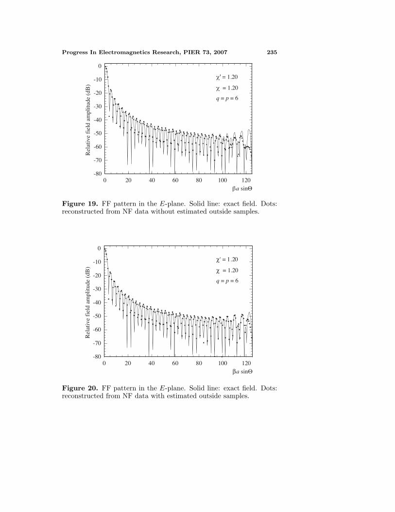
The described technique has been applied to recover theplane-rectangular data needed for the probe compensated NF-FFtransformation and lying in a 100λ × 100λ square grid. Figures 19and 20 report the AUT pattern in the E-plane, reconstructed via theNF-FF transformation without and with estimated outside samples,respectively.

As can be seen, the FF reconstruction obtained by considering theestimated samples is accurate in a significantly wider angular range.In fact, as can be seen in Figs. 19 and 20, the angular extension of thegood FF reconstruction zone increases about 35% for the consideredexample.

It is useful to note that the number of employed NF data in thereported example is 12 151 significantly less than those (30 731) neededby the NF-FF transformation [30]. In particular, the number of extrasamples is 2 355.


-80

-70

-60

-50

-40

-30

-20

-10

0

0 20 40 60 80 100 120

Rel

ativ

e fi

eld

ampl

itude

(dB

)

β a sinΘ

q = p = 6

χ' = 1.20

χ = 1.20

Figure 19. FF pattern in the E-plane. Solid line: exact field. Dots:reconstructed from NF data without estimated outside samples.

-80

-70

-60

-50

-40

-30

-20

-10

0

0 20 40 60 80 100 120

Rel

ativ

e fi

eld

ampl

itude

(dB

)

a sin

q = p = 6

' = 1.20

= 1.20

Figure 20. FF pattern in the E-plane. Solid line: exact field. Dots:reconstructed from NF data with estimated outside samples.


4. CONCLUSION

In this paper, we have proposed an effective technique for extrapolatingthe NF data external to the measurement region in the plane-polarscanning. It allows a significant reduction of the error related tothe truncation of the scan zone. Such a technique relies on thenonredundant sampling representations of the EM fields and onthe OSI expansions of central type, and uses the SVD method forestimating the outside samples. The comparison of this approach witha procedure available in literature and employing the CS expansionshas shown that the proposed technique works better. Numericalsimulations assessing the effectiveness of the extrapolation procedureare reported. In particular, they show that a significant enlargementof the good FF reconstruction zone is attainable when considering theso estimated data.

REFERENCES

1. Bucci, O. M., C. Gennarelli, and C. Savarese, “Representationof electromagnetic fields over arbitrary surfaces by a finiteand nonredundant number of samples,” IEEE Trans. AntennasPropagat., Vol. 46, 351–359, 1998.

2. Bucci, O. M. and G. Franceschetti, “On the spatial bandwidth ofscattered fields,” IEEE Trans. Antennas Propagat., Vol. AP-35,1445–1455, 1987.

3. Bucci, O. M., C. Gennarelli, G. Riccio, and C. Savarese, “Near-field-far-field transformation from nonredundant plane-polar data:effective modellings of the source,” IEE Proc. - Microw., AntennasPropagat., Vol. 145, 33–38, 1998.

4. Bucci, O. M., F. D’Agostino, C. Gennarelli, G. Riccio, andC. Savarese, “NF-FF transformation with plane-polar scanning:ellipsoidal modelling of the antenna,” Automatika, Vol. 41, 159–164, 2000.

5. D’Agostino, F., C. Gennarelli, G. Riccio, and C. Savarese, “Datareduction in the NF-FF transformation with bi-polar scanning,”Microw. Opt. Technol. Lett., Vol. 36, 32–36, 2003.

6. Ferrara, F., C. Gennarelli, R. Guerriero, G. Riccio, andC. Savarese, “An efficient near-field to far-field transformationusing the planar wide-mesh scanning,” J. Electromagn. WavesAppl., Vol. 21, 341–357, 2007.

7. D’Agostino, F., F. Ferrara, C. Gennarelli, G. Riccio, andC. Savarese, “NF-FF transformation with cylindrical scanning


from a minimum number of data,” Microw. Opt. Technol. Lett.,Vol. 35, 264–270, 2002.

8. Bucci, O. M., F. D’Agostino, C. Gennarelli, G. Riccio, andC. Savarese, “Data reduction in the NF-FF transformationtechnique with spherical scanning,” J. Electromagn. Waves Appl.,Vol. 15, 755–775, 2001.

9. D’Agostino, F., C. Gennarelli, G. Riccio, and C. Savarese,“Theoretical foundations of near-field-far-field transformationswith spiral scannings,” Progress In Electromagnetics Research,PIER 61, 193–214, 2006.

10. Gennarelli, C., G. Riccio, F. D’Agostino, and F. Ferrara,Near-field - Far-field Transformation Techniques, Vol. 1, CUES,Salerno, Italy, 2004.

11. Bucci, O. M., C. Gennarelli, and C. Savarese, “Optimalinterpolation of radiated fields over a sphere,” IEEE Trans.Antennas Propagat., Vol. AP-39, 1633–1643, 1991.

12. Slepian, D. and H. O. Pollak, “Prolate spheroidal wave functions,Fourier analysis and uncertainty — I,” Bell Syst. Tech. J., Vol. 40,43–63, 1961.

13. Papoulis, A., “A new algorithm in spectral analysis and band-limited extrapolation,” IEEE Trans. Circuits, Syst., Vol. CAS-22,735–742, 1975.

14. Sabri, M. S. and W. Steenaart, “An approach to band-limitedsignal extrapolation: the extrapolation matrix,” IEEE Trans.Circuits, Syst., Vol. CAS-25, 74–78, 1978.

15. Cadzow, J. A., “An extrapolation procedure for band-limitedsignals,” IEEE Trans. Acoust., Speech, Signal Processing,Vol. ASSP-27, 4–12, 1979.

16. Jain, A. K. and S. Ranganath, “Extrapolation algoritms fordiscrete signals with application in spectral estimation,” IEEETrans. Acoust., Speech, Signal Processing, Vol. ASSP-29, 830–845,1981.

17. Sanz, J. L. C. and T. S. Huang, “Some aspects of band-limitedsignal extrapolation: models, discrete approximation, and noise,”IEEE Trans. Acoust., Speech, Signal Processing, Vol. ASSP-31,830–845, 1983.

18. Sullivan, B. J. and B. Liu, “On the use of singular valuedecomposition and decimation in discrete-time band-limited signalextrapolation,” IEEE Trans. Acoust., Speech, Signal Processing,Vol. ASSP-32, 1201–1212, 1994.


19. Sano, A., “Optimally regularized inverse of singular valuedecomposition and application to signal extrapolation,” SignalProcessing, Vol. 30, 163–176, 1993.

20. Ferreira, P. J. S. G., “The stability of a procedure for the recoveryof lost samples in band-limited signals,” Signal Processing, Vol. 40,195–205, 1994.

21. Landau, H. J., “Extrapolating a band-limited function from itssamples taken in a finite interval,” IEEE Trans. Inf. Theory,Vol. IT-32, 464–470, 1986.

22. Bucci, O. M., G. D’Elia, and M. D. Migliore, “A newstrategy to reduce the truncation error in near-field/far-fieldtransformations,” Radio Science, Vol. 35, 3–17, 2000.

23. Bucci, O. M., G. D’Elia, and M. D. Migliore, “Experimentalvalidation of a new technique to reduce the truncation error innear-field far-field transformation,” Proc. of AMTA 1998, 180–185, Montreal, Canada, 1998.

24. Bolomey, J. C., O. M. Bucci, L. Casavola, G. D’Elia,M. D. Migliore, and A. Ziyyat, “Reduction of truncation errorin near-field measurement of antennas of base-station mobilecommunication systems,” IEEE Trans. Antennas Propagat.,Vol. 52, 593–602, 2004.

25. Golub, G. H. and C. F. Van Loan, Matrix Computations, JohnHopkins University Press, Baltimore, 1996.

26. Press, W. H., S. A. Teukolsky, W. T. Vetterling, andB. P. Flannery, Numerical Recipes, Cambridge University Press,New York, 1999.

27. Hansen, P. C., Rank-deficient and Discrete Ill-posed Problems,SIAM, Philadelphia, USA, 1998.

28. Tikhonov, A. N. and V. Y. Arsenin, Solutions of Ill-posedProblems, Winston, Washington, D.C., USA, 1977.

29. Paris, D. T., W. M. Leach, Jr., and E. B. Joy, “Basic theoryof probe-compensated near-field measurements,” IEEE Trans.Antennas Propagat., Vol. AP-26, 373–379, 1978.

30. Gatti, M. S. and Y. Rahmat-Samii, “FFT applications to plane-polar near-field antenna measurements,” IEEE Trans. AntennasPropagat., Vol. AP-36, 781–791, 1988.

aneffectivetechniqueforreducingthe … · progress in electromagnetics research, pier 73,...

Documents