programación lineal con espacios covariante y

INGENIERÍA Investigación y Tecnología IX. 3. 185-204, 2008(artículo arbitrado)

Programación lineal con espacios covariante ycontravariante. Una perspectiva física y matemática

Linear programming in covariant and contravariantmanifolds. A physical and mathematical perspective

J.L. Urrutia-Galicia 1 , J.C. Alcérreca-Huerta 2 y M.A. Ordaz-Alcántara 3

1 Instituto de Ingeniería, Mecánica Aplicada, Universidad Nacional Autónoma de México, 2 Facultad de Ingeniería, Universidad Nacional Autónoma de México y

3 Facultad de Ciencias, Universidad Nacional Autónoma de MéxicoE-mail: [email protected]

(Recibido: abril de 2006; aceptado: noviembre de 2007)

Resumen

En este artículo se presenta un método de optimización nuevo y diferente a los

utilizados actualmente, como en el “Método Simplex”. Se basa en el empleo de los

espacios covariante y contravariante, ambos espacios biortogonales entre sí, lo

que permite una visualización del problema de optimización tanto física como

matemática. El resultado obtenido proporciona la mejor aproximación de acuerdo a

los datos concentrados en las restricciones del problema, éstas últimas

visualizados como vectores (como un espacio completo o incompleto) y no como

rectas, planos o hiperplanos. Asimismo, con este nuevo método se puede

cuantificar el error generado entre los vectores aproximación y el objetivo, lo que

permite observar y medir la efectividad de la solución propuesta.

Descriptores: Métodos de optimización, espacio covariante (espacio de

columnas) y contravariante (matriz inversa) –vs– método simplex, rotación de

hiperplano, convergencia, solución exacta.

Abstract

In this pa per a new op ti mi za tion method is pre sented. The the o ret i cal back ground

is dif fer ent to that used pres ently as in the case of the “Sim plex Method”. The pre -

sen ta tion is based on the use of the covariant and contravariant spaces, both be -

ing biorthogonal spaces, al low a vi su al iza tion of the op ti mi za tion prob lem from a

phys i cal as well as math e mat i cal points of view. The ob tained re sult pro vides the

best ap prox i ma tion ac cord ing to the data pro vided in the con straints of the pro-

blem, which are vi su al ized like vec tors and not like straight lines, planes or

hyperplanes. Also, in this new method the er ror gen er ated be tween the ap prox i ma -

tion and the ob jec tive vec tors can be mea sured, which al lows to ob serve and prove

the ac cu racy of the pro posed so lu tion.

Key words: Op ti mi za tion meth ods, covariant and contravariant spaces –vs– sim -

plex method, hyperplane ro ta tion, con ver gence, ex act so lu tion.

InvesInves tiga

tiga

cionescionesEstudios eEstudios e

RecientesRecientes

Introducción

Bien es sabido que dentro de los márgenes decualquier problema práctico, lo que se busca es elmejor empleo de los recursos humanos, comer-ciales, laborales, tecnológicos, etc., de tal maneraque se logre la distribución y uso más ventajoso delos mismos. Es por eso que surgen modelos quetratan de optimizar los recursos disponibles, yasean maximizando ganancias o minimizando gas-tos o pérdidas.

Los problemas de optimización se presentan enmúltiples disciplinas, teniendo en común una meta por alcanzar, sujeta a restricciones que influyen demanera directa limitando las posibles soluciones al problema de maximizar o minimizar el objetivo pro-puesto. Por ejemplo; en administración, un obje-tivo muy común es el de maximizar las ganancias,tomando en cuenta los límites impuestos por lostiempos de operación, costos de producción, ca-pital disponible para la inversión, entre otros fac-tores; a nivel industrial, los gastos de operación seencuentran sujetos a la eficiencia de la maqui-naria, a los productos manufacturados o la llegadade materia prima.

Fue alrededor de la Segunda Guerra Mundial en que se iniciaron los primeros pasos hacia la bús-queda de modelos matemáticos que resolvieranlos problemas de optimización, uno de estos mo-delos surge con el fin de resolver los problemas deasignación de recursos por parte de la fuerza aérea estadounidense. George B. Dantzig, miembro delproyecto SCOOP (Scientific Computation of Opti-mun Programs) de la fuerza aérea de E.U., fuequien diseñó el método simplex de solución en1947, modelo que sigue siendo ampliamente utilizado hasta nuestros días (Fraleigh y Beauregard,1989a).

El desarrollo de la programación lineal, es con-siderado por mucha gente como uno de los avan-ces científicos más importantes de la segundamitad del siglo XX. De hecho, una proporción im-portante de todo el cálculo científico que se lleva a

cabo por computadoras se dedica al uso de la pro-gramación lineal y a técnicas íntimamente relacio-nadas, estimándose en un 25%, de acuerdo a unestudio de la IBM (Marrero et al, 2006).

Un modelo de programación lineal, como el mé- todo simplex o el que se desarrolla en este artículoempleando los espacios covariante y contrava-riante, tratan de proporcionar una vía eficientepara determinar una solución óptima para losproblemas de maximización o minimización de unobjetivo dadas determinadas restricciones.

Método Simplex

Análisis gráfico

El método simplex busca resolver problemas deprogramación lineal; dicho método, cuando poseedos variables de optimización es visto de maneragráfica como la traza de planos dados por lasecua- ciones de las restricciones, generándose unpolí- gono al graficar todas éstas. Al desplazar latraza del plano de la función objetivo hacia elpolígono mencionado anteriormente, se obtieneuna solu- ción óptima en el primer punto en queambos se intersectan.

Para mostrar lo anterior, se toma un ejemplo de Fraleigh y Beauregard (1989b), donde se proponeel siguiente problema:

Ejemplo 1

Sea una compañía maderera que posee dos talle-res de contrachapado, donde se producen los tresmismos tipos de tableros, hallar el número de díasque debe operar cada taller durante un semestrepara proporcionar de la manera más económicalos tableros requeridos. La tabla 1 muestra la pro-ducción y costo diarios por taller.

186 INGENIERIA Investigación y Tecnología FI-UNAM

Programación lineal con espacios covariante y contravariante. Una perspectiva física y matemática

Vol.IX No.3 -julio-septiembre- 2008 187

J.L. Urrutia-Galicia, J.C. Alcérreca-Huerta y M.A. Ordaz-Alcántara

Con los datos contenidos en la tabla podemos de-terminar tanto la función objetivo como las restric-ciones que intervienen en el problema:

Minimizar C=3000x1 +2000x2 (1)

condicionado a las siguientes restricciones:

100x1 +20x2 ³ 200040x1 +80x2 ³ 3200 (2)60x1 +60x2 ³ 3600

y con x x1 20 0³ ³, .

En la figura 1, se encuentra achurado el espacio solución limitado por las gráficas de las trazas de

los planos de las restricciones; asimismo, con línea punteada, se encuentra graficada la pendiente dela función objetivo. Al desplazar la función objetivohacia el polígono e intersectarse, como se muestra en la figura 2, se obtiene la solución óptima, queresulta ser x1 10= y x2 50= .

Al sustituir los valores de x1 y x2 en la funciónobjetivo de costo inicialmente planteada, se tieneque el costo mínimo de producción sería:

C

C

= +

=

3000 10 2000 50

130 000

( ) ( )

$ (3)

Algoritmo del método simplex

La forma analítica del método simplex funciona demanera similar al método gráfico, la diferencia ra-dica en que para buscar la intersección entre el polí-gono y la traza de la función objetivo se recorrenlas aristas del polígono o poliedro generado por lasrestricciones, siendo los vértices o puntos esquinalas soluciones factibles al problema, sin necesidadde probar todos los puntos esquina. Para iniciar elrecorrido a lo largo del polígono o poliedro, es ne-cesario añadir a las restricciones, representadascon igualdades o desigualdades como: variables

Tabla 1

Tipo decontrachapado

Producción por día DemandasemestralTaller 1 Taller 2

1 100 20 2000

2 40 80 3200

3 60 60 3600

Costos diarios $3000 $2000

Figura 1

de holgura, variables excedentes y variables arti-ficiales, esto último con el motivo de convertir to-das las desigualdades de las restricciones en igualdades, además de que con ello se genera un con-junto de variables básicas y otro de variables nobásicas con lo que se puede empezar dicho recorrido.

Primeramente se comienza en cualquier puntoesquina, para después moverse hacia cualquierotro adyacente, de manera que la función objetivose incremente lo más rápidamente posible (Fra-leigh y Beauregard, 1989c), para hacer lo anterior, una variable básica se hace no básica y viceversa,disponiendo del conjunto de variables no básicasgenerado al introducir las variables de holgura, exce-dentes y artificiales. Un óptimo se alcanza cuandoel valor de la función es máximo y ninguna otrasolución básica factible puede ser encontrada(Bhatti, 2000).

En caso de que se busque minimizar una fun-ción objetivo, cuyas restricciones sean de la for-ma Ax b£ , con b ³ 0, se hace uso de la siguienteexpresión:

[Mínimo de f x( )]=– [Máximo de – f x( )] (4)

Empleando el problema mostrado anteriormenteen el método gráfico, se ejemplifica de manerabreve, la forma de resolución a través del algoritmo del método simplex.

Una vez que se han obtenido la función objetivo(1) y las restricciones del problema (2), se procede a convertir las desigualdades de las restriccionesen igualdades por medio de la adición, en este ca-so, de variables excedentes y artificiales, por lo que se tiene:

100 20 2000

40 80 3200

60 60

1 2 1 1

1 2 2 2

1 2

x x y q

x x y q

x x

+ - + =

+ - + =

+ - + =y q3 3 3600

(5)

Dado que se desea minimizar la funciónobjetivo C (1) es necesario utilizar la expresiónmostrada en (4). Aún cuando las restriccionesdeban tener la forma Ax b£ , la cuestión se veresuelta tras la añadidura de las variablesexcedentes.

Las variables artificiales deberán tomar el valorcero para obtener una solución factible al proble-ma original. Entonces el problema de minimizar C



Figura 2

se transforma en un problema de maximizar P=–C, siendo la nueva función objetivo:

P x x Mq Mq Mq= - - - - -3000 20001 2 1 2 3 (6)

Donde M es un número muy grande, lo que permite que la función objetivo no se pueda optimizarsin que los qi tomen el valor cero, como se men-cionó arriba.

Una vez modificadas las restricciones y la fun-ción objetivo, se elabora una tabla inicial donde sehallan concentradas todas las variables de las res-tricciones (5) y el objetivo.

Para la formación de la última fila de la tabla inicial, correspondiente al objetivo, se tiene que parauna columna etiquetada con una variable xi, seañade en la fila objetivo el negativo del producto de M por la suma de coeficientes que multiplican a xi

en las restricciones. En las columnas etiquetadascon yi se añade M, mientras que en las etiquetadas con qi se escriben ceros; en la última columna setiene el negativo del producto de M por la suma delos términos independientes de las restricciones.

A continuación, mediante un tipo de reducción deGauss-Jordan, las variables básicas se hacen nobásicas y viceversa, hasta que se obtiene la so-lución óptima al no quedar registros negativos dela fila objetivo y si ninguna variable artificial es bá-sica o si todas las variables artificiales básicas tienenvalor cero, como se muestra en las tablas 2 a 4.

En la tabla 4, se encuentran los valores de x1 10= y x2 50= , obteniéndose el máximo de Pigual con -130000. Al emplear nuevamente la ex-presión señalada en (4), se tiene que el costo mí-nimo de producción es de $130000, solución quese obtuvo con el método gráfico.

No obstante, hay que destacar que aunque sesatisficieron las restricciones del problema, se puede observar en la última columna de la tabla 4 quela variable excedente y2 tiene un valor igual con1200, indicativo de una sobreproducción del con-trachapado 2 producido por ambos talleres y que,al comparársele con la demanda semestral del pro-ducto que es igual con 3200 representa el 37.5%de la ya mencionada demanda, por lo que seríarecomendable encontrar una solución alternativa.



Tabla inicial

x1 x2 y1 y2 y3 q1 q2 q3

q1 100 20 -1 0 0 1 0 0 2000

q2 40 80 0 -1 0 0 1 0 3200 ~

q3 60 60 0 0 -1 0 0 1 3600

P3000 2000 0 0 0

-200M -160M M M M -8800M

Tabla 2

x1 x2 y1 y2 y3 q1 q2 q3

x1 1 0.2 -0.01 0 0 0.01 0 0 20

~ q2 0 72 0.4 -1 0 -0.4 1 0 2400 ~

q3 0 48 0.6 0 -1 -0.6 0 1 2400

P0 1400 30 -30 0 0 -60000

-120M -M M M 2M -4800M

Método con espacios covariante ycontravariante

Este método se basa principalmente en una visiónfísica y matemática de los problemas, por lo quelas soluciones encontradas responden a diversassituaciones planteadas en la realidad. Como severá, las variables de holgura, excedentes y artifi-ciales, que son introducidas en el método simplex,no representan absolutamente nada al utilizar elnuevo método, ya que no forman parte del proble-ma original.

Urrutia (2003), mostró la metodología parainvertir matrices rectangulares y para modificaróptimamente las restricciones (cuando esto esposible o mandatario), la cual tiene aplicación para la optimización de funciones dadas determinadasrestricciones.

Con el motivo de hacer hincapié en el trata-miento físico que se hará al problema, las restric-ciones (2) del problema presentado, son escritasde la siguiente manera:

x x1 2

100

40

60

20

80

60

2000

3200

3

×

æ

è

ççç

ö

ø

÷÷÷

+ ×

æ

è

ççç

ö

ø

÷÷÷

³

600

æ

è

ççç

ö

ø

÷÷÷ (7)

donde las ecuaciones de las restricciones sonvistas como una combinación lineal de dos vec-tores en la que las variables de optimización x1 y x2

son escalares que multiplican a los vectores:

~( )f1 = 100 40 60 T y

~( )f2 20 80 60= T

respectivamente, para obtener como objetivo

~ ( )v T= 2000 3200 3600

Por otra parte, el fin sigue siendo minimizar lafunción costo mostrada en (1):

C=3000x1 +2000x2

Las restricciones del problema, en este caso,son de la forma Ax b³ ; sin embargo, lo deseable



Tabla 3

x1 x2 y1 y2 y3 q1 q2 q3

x1 1 0 -0.0111 0.0028 0 0.0111 -0.0028 0 13.33

~ x2 0 1 0.0056 -0.0139 0 -0.0056 0.0139 0 33.33 ~

q3 0 0 0.3333 0.6667 -1 -0.3333 -0.6667 1 800

P0 0 22.222 19.44 -22.22 -19.44 0 -106667

-0.333M -0.667M M +1.333M +1.667M -800M

Tabla 4

x1 x2 y1 y2 y3 q1 q2 q3

x1 1 0 -0.0125 0 0.0042 0.0125 0 -0.0042 10

~ x2 0 1 0.0125 0 -0.0208 -0.0125 0 0.0208 50

y2 0 0 0.5 1 -1.5 -0.5 -1 1.5 1200

P0 0 12.5 0 29.17 -12.5 -29.17 -130000

+M M +M

en un problema de optimización es lograr la igual-dad en las restricciones, es decir, que se obtengala solución a Ax b= o en donde Ax b- resulta míni- ma. El método con espacios covariante y contra-variante (de cálculo tensorial) busca cumplir condicha igualdad, por lo tanto, al aplicar el método se sustituye el signo de desigualdad y se cambia porel de igualdad en miras de conseguir la mejor so-lución y de emplear sin dificultades la metodo-logía para invertir matrices rectangulares. Para pa-sar de la desigualdad a la igualdad no es nece-sario añadir ningún tipo de variable como sucedeen el método Simplex, sino que se busca resolverel problema con las variables presentes en el pro-blema original. Así entonces, las restricciones deeste problema se escriben como sigue:

x x1 2

100

40

60

20

80

60

2000

3200

3

×

æ

è

ççç

ö

ø

÷÷÷

+ ×

æ

è

ççç

ö

ø

÷÷÷

=

600

æ

è

ççç

ö

ø

÷÷÷ (8)

A continuación se agrupan los vectores ~

,~

f f1 2 ylas variables de optimización como se muestra:

100

40

60

20

80

60

2000

3200

3600

1

2

æ

è

ççç

ö

ø

÷÷÷

×æ

èçç

ö

ø÷÷ =

æx

xè

ççç

ö

ø

÷÷÷ (9)

La matriz que agrupa a los vectores ~

,~

f f1 2 ,(pertenecientes al espacio covariante) se le desig-nará con el nombre de A; al conseguir la inversapor la izquierda de dicha matriz (A-1) escrita en laforma estándar

A- =-

-1 0 010714 0 003571 0 00119

0 007143 0 010714 0 004

. . .

. . . 762

æ

èçç

ö

ø÷÷ (10)

se obtienen los vectores

~( . . . )f 1 = -0 0101714 0 003571 0 00119 T

~( . . . )f 2 = -0 007143 0 010714 0 004762 T

que por conveniencia en la visualización de lamatriz conformada por vectores es mejor escribir:

AT- = -

-1

0 010714

0 003571

0 00119

0 007143

0 010714

0 00

.

.

.

.

.

. 4762

æ

è

ççç

ö

ø

÷÷÷ (11)

Al multiplicar (8) por los vectores ~f 1 y

~f 2 (per-

tenecientes al espacio contravariante) servirán pa-ra hallar los valores de las variables de optimi-zación:

(~ ~ ~)

~x x1 1 2 2

1× + × = ×f f n f (12)

x x1 2

100

40

60

20

80

60

2000

3200

3

×

æ

è

ççç

ö

ø

÷÷÷

+ ×

æ

è

ççç

ö

ø

÷÷÷

=

600

0 010714

0 003571

0 00119

æ

è

ççç

ö

ø

÷÷÷

é

ë

êêê

ù

û

úúú

× -

æ

è

.

.

.

ççç

ö

ø

÷÷÷

(~ ~ ~)

~x x1 1 2 2

2× + × = ×f f n f (13)

x x1 2

100

40

60

20

80

60

2000

3200

3

×

æ

è

ççç

ö

ø

÷÷÷

+ ×

æ

è

ççç

ö

ø

÷÷÷

=

600

0 007143

0 010714

0 004762

æ

è

ççç

ö

ø

÷÷÷

é

ë

êêê

ù

û

úúú

×

-

-

.

.

.

æ

è

ççç

ö

ø

÷÷÷

al efectuar las operaciones señaladas en (12) y(13), se obtienen los valores de x1= 14.285714 yx2= 37.142857 que, al ser sustituidos primero enla ecuación (2) nos daría la siguiente producción:

14 2857

100

40

60

37 1428

20

80

60

2

. .

æ

è

ççç

ö

ø

÷÷÷

+

æ

è

ççç

ö

ø

÷÷÷

=

171 426

3542 852

3085 71

.

.

.

æ

è

ççç

ö

ø

÷÷÷

En seguida se sustituyen x1= 14.285714 y x2=37.142857 en la función costo (1) proporcio-nando el valor mínimo de costos de producción y el cual resulta ser menor al obtenido con el métodosimplex:



C = +3000 14 285714 2000 37 142857( . ) ( . ) C = $ .117142 86 (14)

Haciendo la consideración de que se trabajan 8horas por día, los valores de x1 y x2 al ser frac-cionarios significan que se deben trabajar 14 díasnormales laborables más 2.25 horas extras paraterminar la producción en el taller 1 y 37 días con1.14 horas en el taller 2.

Como se puede apreciar en la figura 3, losvectores x1 1×

~f y x2 2×

~f se encuentran en un plano

diferente al del objetivo ~n; por lo que no se puedegenerar una solución exacta, siendo el mínimoerror la proyección del objetivo sobre el planogenerado por

~f1 y

~f2 .

Aun cuando ya han sido encontrados los valores de las variables de optimización, es necesario en-tender qué es lo que se hizo matemáticamente,por ello, se recurre a la explicación física que vaíntimamente ligada con los resultados y el proce-dimiento realizado. Así, al sustituir en la ecuación(8) los valores de x1 y x2 obtenidos con este mé-todo, se obtiene el vector aproximación

~ ( )p T= 2171 3543 3086

Este último vector (~p ) resulta de aplicar la ley delparalelogramo de composición de fuerzas de física, también llamada Principio de Stevin, entre los vec-tores x1 1×

~f y x2 2×

~f , y que se expresa matemá-

ticamente en las ecuaciones (15) y (16).

14 285714

100

40

60

37 142857

20

80

60

. .

æ

è

ççç

ö

ø

÷÷÷

+

æ

è

ççç

ö

ø

÷÷÷

=

2171 429

3542 857

3085 714

2000

3200

3600

.

.

.

æ

è

ççç

ö

ø

÷÷÷

»

æ

è

ççç

ö

ø

÷÷÷ (15)

1428 572

571 429

857 143

742 857

2971 428

22

.

.

.

.

.

æ

è

ççç

ö

ø

÷÷÷

+

28 571.

æ

è

ççç

ö

ø

÷÷÷

=

(16)2171 429

3542 857

3085 714

2000

3200

3600

.

.

.

æ

è

ççç

ö

ø

÷÷÷

»

æ

è

ççç

ö

ø

÷÷÷

Al comparar la producción obtenida (16) de loscontrachapados 1, 2 y 3 con la demandada por el



22

~f×x

Aproximación

Objetivo Error

Figura 3

vector objetivo ~ ( )n = 2000 3200 3600 T , se tiene una sobreproducción del 8.6% y 11.1% en elcontrachapado 1 y 2 respectivamente, y una sub-producción del 14.3% del tercer contrachapado.

Esta solución, siendo una mala aproximación,es sin embargo la mejor, pues aun sumando losporcentajes de sobreproducción y subproducción,obtenidos previamente, no superan al error del37% de sobreproducción que representa optar porla solución calculada con el método simplex; ade-más, nada se puede hacer bajo las actuales polí-ticas de producción impuestas por los números enlas columnas de la ecuación (2).

El vector aproximación ~p obtenido, resulta ser la proyección del vector objetivo:

~ ( )n = 2000 3200 3600 T

sobre el plano generado por los vectores ~f1 y

~f2 .

Se puede observar en la figura 3 que el vector error debe ser ortogonal al vector aproximación con elmotivo de que el error sea mínimo y, por tanto,obtener la mejor solución al problema.

Para comprobar la ortogonalidad entre losvectores aproximación y error, y de que se obtuvocomo consecuencia la mejor solución posible, sedebe efectuar un producto punto entre dichos vec-tores, de tal modo que el resultado sea cero.

La diferencia entre los vectores objetivo y apro-ximación da lugar al vector error

~ ~ ~e v p= - (17)

cuya característica, como se dijo anteriormente, es que debe de ser ortogonal al plano donde selocalizan

~f1 y

~f2 , lo cual significa que se obtuvo la

mejor aproximación, pues cualquier otra solucióngenerará un vector error mayor en magnitud, quees absolutamente indeseable.

Al calcular el vector error generado con estemétodo (~eC ) se obtiene lo siguiente:

~eC =

2000

3200

3600

2171 429

3542 857

3085 714

æ

è

ççç

ö

ø

÷÷÷

-

æ

è

ç.

.

.

çç

ö

ø

÷÷÷

=

-

-

æ

è

ççç

ö

ø

÷÷÷

171 429

342 857

514 286

.

.

.

(18)

y cuando se efectúa el producto punto entre ~eC y el vector aproximación ~p se obtiene el siguiente re-sultado:

-

-

æ

è

ççç

ö

ø

÷÷÷

×

171 429

342 857

514 286

2171 429

3542 857

.

.

.

.

.

3085 714

0

.

æ

è

ççç

ö

ø

÷÷÷

= (19)

con lo que se demuestra la ortogonalidad entre lasolución obtenida ~p y el error ~eC con el método deespacios covariante y contravariante al generar elmínimo error posible.

Si se calcula el vector error que se genera alemplear la solución obtenida con el método sim-plex (~eS ), se obtendría primeramente que el vectoraproximación sería

10

100

40

60

50

20

80

60

2000

4400

360

æ

è

ççç

ö

ø

÷÷÷

+

æ

è

ççç

ö

ø

÷÷÷

=

0

2000

3200

3600

æ

è

ççç

ö

ø

÷÷÷

»

æ

è

ççç

ö

ø

÷÷÷ (20)

y empleando (16), se tiene

~eS =

2000

3200

3600

2000

4400

3600

0

12

æ

è

ççç

ö

ø

÷÷÷

-

æ

è

ççç

ö

ø

÷÷÷

= - 00

0

æ

è

ççç

ö

ø

÷÷÷ (21)

Una vez que han sido calculados los vectoreserror que se generan con ambos métodos, pormedio del concepto de norma de un vector sepueden comparar ambos resultados de donde setiene lo siguiente:

~ ( ) ( ) ( ) .eC = - + - + =171 343 514 641 4272 2 2

~ ( ) ( ) ( )eS = + - + =0 1200 0 12002 2 2 (22)



\ <~ ~e eC S (23)

En la figura 4 se pueden observar las dos soluciones que se generan con ambos métodos desdeel punto de vista físico, además del resultadoobtenido en (23). Para no confundir entre las solu-ciones encontradas, los valores de las variables deoptimización del método simplex se denotan con x S1 y x S2 , asimismo, para el vector aproximaciónse le designa con el nombre de ~pS , mientras quelos encontrados por medio de los espacioscovariante y contravariante son denotados por x C1 ,x C2 y el vector aproximación por ~pC .

Restricciones xi

³ 0

Para el último ejemplo, no se hizo uso de lasrestricciones x x1 20 0³ ³, , debido al enfoque fí-sico y gráfico mostrado con anterioridad; sin em-bargo, siendo estrictos estas dos restricciones de-ben de ser consideradas dentro del conjunto derestricciones del problema por lo que se tendría elsiguiente planteamiento global:

minimizar C x x= +3000 20001 2

sujeto a

100 20 20001 2x x+ ³40 80 32001 2x x+ ³60 60 36001 2x x+ ³ (24)1 0 01 2x x+ ³0 1 01 2x x+ ³

por lo que ahora se tendría, escrito a manera decombinación lineal y en la forma Ax b= :

x x1 2

10

40

60

1

0

20

80

60

0

1

æ

è

çççççç

ö

ø

÷÷÷÷÷÷

+

æ

è

çççççç

ö

ø

÷÷÷÷÷÷

=

æ

è

çççççç

ö

ø

÷÷÷÷÷÷

2000

3200

3600

0

0

(25)

de donde se observa que los vectores

~f1 =( )100 40 60 1 0 T

y~f2 =( )20 80 60 0 1 T



22

~f×Cx

Ce~

Se~

Sp~Cp~

22

~f×Sx

Objetivo

11

~f×Cx

11

~f×Sx

Figura 4

pertenecen al espacio Â5 , por lo que su represen-tación gráfica resulta imposible, no así su inter-pretación física.

Siguiendo con la metodología de los espacioscovariante y contravariante tenemos que

~

.

.

.

.

.

f 1

3

3

4

0 010712

3 57 10

1 191 10

1 289 10

1 091 1

=

-

-

-

-

-

x

x

x

x 0 4-

æ

è

ççççççç

ö

ø

÷÷÷÷÷÷÷

Y

(26)

~

.

.

.

.

.

f 2

3

3

4

7 14 10

0 0107119

4 761 10

1 091 10

1 8844

=

-

-

-

-

-

x

x

x

x10 4-

æ

è

ççççççç

ö

ø

÷÷÷÷÷÷÷

que al multiplicar (25) de manera similar a la mos-trada en (12) y (13), se obtienen los valores de x1=

14.287924 y x2 = 37.137416.

Empleando estos nuevos valores y sustituyén-dolos en la función costo (1) se tiene:

C = +3000 14 287924 2000 37 137416( . ) ( . ) (27)C = $ .117138 61

que resulta ser un valor más pequeño en costosrespecto al valor obtenido en (14).

El vector aproximación resulta ahora de:

~ ( . .p = 2171 541 3542 51

3085 52 37 137 14 288. . . )T

con lo que se puede calcular el vector error y portanto, la norma del mismo:

~

.

.

eC =

æ

è

çççççç

ö

ø

÷÷÷÷÷÷

-

2000

3200

3600

0

0

2171 541

3542 51

3085 52

37 137

14 288

171 541

342 5

.

.

.

.

.

æ

è

çççççç

ö

ø

÷÷÷÷÷÷

=

-

- 1

514 48

37 137

14 288

.

.

.

-

-

æ

è

çççççç

ö

ø

÷÷÷÷÷÷

(28)

~ .eC = 642 66 (29)

La nueva solución genera un error mayor, de-bido a la introducción de las nuevas restricciones.Pese a lo anterior se sigue cumpliendo la ecuaciónmostrada en (30), así como la ortogonalidad entrelos vectores aproximación y error

~ ~e pC × = 0 (30)

Dado que ~f1 y

~f2 son los vectores que forman

la combinación lineal en las restricciones del pro-blema para cumplir al objetivo ~n, ecuaciones (8) y(25), es de esperar que si se cambian los valoresque conforman los vectores antes mencionados lasolución al problema también lo haga. Las restric-ciones del problema son las que limitan en mayormedida las posibles soluciones al mismo.

La solución del problema de optimización quese obtiene con el método de espacios covariante ycontravariante, gira esencialmente en torno de laeficiencia en el cumplimiento de las restricciones ydel error que se genera al verificarlas. Mientrastanto, la función objetivo funge como un resultadofinal cuantitativo de la calidad de las decisionestomadas, es decir, la función objetivo engloba demanera numérica las consecuencias de tomar encuenta los valores que pretenden satisfacer lasrestricciones propuestas.

La visualización y el entendimiento de los pro-blemas de optimización, se refleja inmediatamente en las decisiones tomadas, así como en la capa-cidad de reacción de una empresa. El siguienteejemplo muestra que aún cuando el objetivo no sepuede alcanzar, la cuantificación del error per-mite tomar decisiones de qué tan eficaz es la so-lución presentada para su uso o, definitivamente,



cancelar los planes originales de producción yefectuar cambios mínimos en los mismos que per-mitan alcanzar el objetivo sin error alguno, refleján- dose todo ello en la función objetivo que se propone.

Ejemplo 2

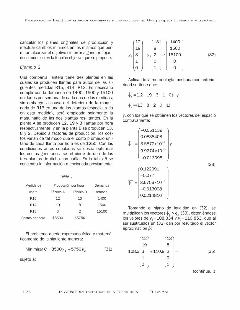
Una compañía llantera tiene tres plantas en lascuales se producen llantas para autos de las si-guientes medidas R15, R14, R13. Es necesariocumplir con la demanda de 1400, 1500 y 15100unidades por semana de cada una de las medidas; sin embargo, a causa del deterioro de la maqui-naria de R13 en una de las plantas (especializadaen esta medida), será empleada solamente lamaquinaria de las dos plantas restantes. En laplanta A se producen 12, 19 y 3 llantas por horarespectivamente, y en la planta B se producen 13,8 y 2. Debido a factores de producción, los cos-tos varían de tal modo que el costo promedio uni-tario de cada llanta por hora es de $250. Con lascondiciones antes señaladas se desea optimizarlos costos generados tras el cierre de una de lastres plantas de dicha compañía. En la tabla 5 seconcentra la información mencionada previamente.

El problema queda expresado física y matemá-ticamente de la siguiente manera:

Minimizar C y y= +8500 57501 2 (31)

sujeto a:

y y1 2

12

19

3

1

0

13

8

2

0

1

æ

è

çççççç

ö

ø

÷÷÷÷÷÷

+

æ

è

çççççç

ö

ø

÷÷÷÷÷÷

³

æ

è

çççççç

ö

ø

÷÷÷÷÷÷

1400

1500

15100

0

0

(32)

Aplicando la metodología mostrada con anterioridad se tiene que:

~f1 =( )12 19 3 1 0 T y ~f2 =( )13 8 2 0 1 T

y, con los que se obtienen los vectores del espaciocontravariante:

~

.

.

.

.

.

f 1 3

3

0 051139

0 0838408

3 5872 10

9 9274 10

0 013

=

-

-

-

-

x

x

098

æ

è

ççççççç

ö

ø

÷÷÷÷÷÷÷

y

(33)

~

.

.

.

.

.

f 2 3

0 122091

0 077

3 6706 10

0 013098

0 0214816

=

-

-

æ

è

ç

-x

ççççç

ö

ø

÷÷÷÷÷÷

Tomando el signo de igualdad en (32), semultiplican los vectores

~f1 y

~f2 (33), obteniéndose

los valores de y1=108.334 y y2=110.853, que alser sustituidos en (32) dan por resultado el vectoraproximación ~p :

108 3

12

19

3

1

0

110 9

13

8

2

0

1

. .

æ

è

çççççç

ö

ø

÷÷÷÷÷÷

+

æ

è

çççççç

ö

ø

÷÷÷÷÷÷

= (35)

(continúa...)



Tabla 5

Medida de Producción por hora Demanda

llanta Fábrica A Fábrica B semanal

R15 12 13 1400

R14 19 8 1500

R13 3 2 15100

Costos por hora $8500 $5750

2741 103

2945 174

546 709

108 334

110 853

.

.

.

.

.

æ

è

çççççç

ö

ø

÷÷÷÷÷÷

»

æ

è

çççççç

ö

ø

÷÷÷÷÷÷

1400

1500

15100

0

0

(35)

Con el vector aproximación ~p y empleando laexpresión (17) se obtiene el vector error:

~ ( . . .e = - -1341 103 1445 174 14553 291 - -108 334 110 853. . )T (36)

Para medir qué tan grande o significativo es elerror respecto de la aproximación y del objetivo

~ ( )n = 1400 1500 15100 0 0 T

es necesario recordar que el vector aproximación ~py el vector error ~e son ortogonales, por lo que segenera un triángulo rectángulo en donde cada lado tiene de magnitud la norma del vector que loforma, es por eso que se calculan las normas decada vector:

~ .e = 14687 05

~ .p = 4063 325 (37)

~ .n = 15238 77

En la figura 5 se muestra el triángulo formadopor las normas de los vectores (37) donde es claroque el vector error ~e resultante es más grande quela mejor aproximación ~p que se pueda encontrar,debido a las condiciones iniciales planteadas

~f1 y

~f2 .

El error generado es consecuencia directa delángulo que existe entre el hiperplano formado porlos vectores

~f1 y

~f2 , y el vector objetivo ~n, el cual

se puede calcular con ayuda de la siguiente ex-presión:

~ ~ ~ ~ cos( )p p× = × ×n n a (38)

de donde se obtiene el valor de a = °74 5353. .

Dicho ángulo, así como la magnitud del vectorerror, son valores que deben tenerse muy en cuenta en la toma de decisiones, pues son indicadoresde la viabilidad o inviabilidad de la solución ob-tenida. La factibilidad de la solución es conseguida en el método simplex por medio de un análisis desensibilidad; sin embargo, en el caso del métodocon espacios covariante y contravariante, el ángulo indica de manera directa dicha factibilidad puestoque el ángulo representa la relación entre el vector objetivo ~n y la aproximación ~p contenida en elhiperplano formado por los

~f

i. Por ejemplo, si se

tuviese que el ángulo a es aproximado o tiende a90º, se sabría que el vector aproximación tenderíaal vector cero (~

~p ® 0), y dado que en el cálculo

del vector aproximación se emplearon los esca-lares que proporcionan la solución al problema, setendría una total inviabilidad de la solución, mismoresultado que arrojarían los análisis de sensibilidad del método simplex.



a

p~

v~

e~

Figura 5

Regresando al problema, cuando los valores de y1

y y2 son sustituidos en la función costo (31) setiene que:

C = +8500 108 3 5750 110 9( . ) ( . ) (39)C = $ .1558 225 0

Cuando se procede a la resolución de esteproblema aplicando el método simplex, se obtieneque y1= 5033.33 y y2 = 0.

Con las restricciones escritas de la forma mos-trada en (32) se calculan los vectores aproxima-ción (~pS ) y error (~eS ):

~

.

, ~p eS S=

æ

è

çççççç

ö

ø

÷÷÷÷÷÷

=

-60400

95633

15100

5033 3

0

59000

94133

0

5033 3

0

-

-

æ

è

çççççç

ö

ø

÷÷÷÷÷÷

.

(40)

de donde se tiene que ~ .eS = 111208 9, que al ser comparada con la norma del vector error delmétodo con espacios covariante y contravariante(37) se observa una contrastante diferencia.

Al sustituir los valores de y1 y y2 obtenidos con la solución del simplex, se tiene que la funciónobjetivo (31) asumiría el siguiente valor

C = +8500 5033 33 5750 0( . ) ( )

C=$42 783.33 (41)

que no resulta nada agradable, sobretodo si se lecompara con el resultado obtenido en (39).

Analizando las soluciones presentadas, al apli-car el método simplex, se satisfaría la demanda dellantas a un costo bastante elevado (41), ademásde que se tendría que cerrar la planta B de lacompañía, cuestión que no sería muy aceptabledebido a los costos que esto podría representar.

Al mismo tiempo, los enormes excedentes deproducción de llantas R15 y R14 en la plantarestante podrían desencadenar otros problemasrelacionados con la maquinaria, como puede sersu deterioro inmediato (factor que propició elcierre de la planta C), o una acumulación de in-ventario que se ve reflejado en costos por alma-cenamiento.

Por otro lado, comparando los resultados obte-nidos por el método de espacios covariante y con-travariante se obtiene un valor muy bajo en cuantoal costo de producción de llantas (39), además deque ambas plantas A y B se mantienen operandoconjuntamente sin poner en riesgo la maquinariaque en ellas se dispone. Respecto a los excesos en la producción de llantas R15 y R14 que son de1341 y 1445 respectivamente, y que se observanen los dos primeros elementos del vector error(36), no resultan ser tan grandes como los obte-nidos en el método simplex: 59000 y 94133 paralas llantas R15 y R14, y que se pueden observar en los dos primeros elementos del vector ~eS en laecuación 40.

Mientras tanto, la falta de producción de 14553 llantas R13 que se obtiene por el método conespacios covariante y contravariante, y que semuestra en el tercer elemento del vector error(36), es el reflejo del cierre de la planta C espe-cializada en este ramo y de la incapacidad de lasplantas A y B para poder suplirla.

Dado que ninguna de las dos soluciones pro-puestas resultan ser viables: la del método sim-plex por los altos costos que representa tomardicha solución y la del método con espacioscovariante y contravariante por no cumplir satis-factoriamente con la demanda; debe consi-derarse seriamente un cambio en los niveles deproducción actuales a fin de completar la de-manda propuesta inicialmente y lograr un míni-mo en los costos de producción.



Rotación de planos (Cambios deproducción)

Aunque el método con espacios covariante y con-travariante no satisface la demanda, posee unaventaja amplia sobre el método simplex, pues pro-porciona una visualización física del problema, enla cual el resultado obtenido (~)p es la proyeccióndel vector ~n sobre el hiperplano generado por losvectores

~f1 y

~f2 . Puesto que los vectores

~f1 ,

~f2 , y

~n no son coplanares, no se puede obtener unasolución exacta al problema; sin embargo, si losvectores

~f1 y

~f2 son proyectados sobre el hiper-

plano que contiene al vector ~n, se logra que todoslos vectores sean coplanares y alcanzar así unasolución exacta.

La metodología presentada por Urrutia-Galicia(2003), permite realizar lo anterior con base enque el hiperplano que contiene a los vectores

~f1 y

~f2 será rotado un ángulo q hasta alcanzar la posi-

ción en la que el vector ~n se halle contenido enéste, posteriormente los vectores

~f1 y

~f2 son pro-

yectados en el nuevo hiperplano que contiene alvector ~n, (Figura 6).

La rotación del hiperplano, así como la pro-yección de los vectores

~f1 y

~f2 sobre el mismo,

representan los cambios mínimos requeridos enlos niveles de producción a fin de satisfacer lademanda planteada inicialmente, con lo que no seproducirá error alguno después de efectuar dichoscambios.

Continuando con el ejemplo de la compañíallantera, la cual tiene serios problemas con su pro-ducción, es urgente y necesario el cambio en losniveles de producción a fin de sobrellevar su situa-ción actual. Empleando los resultados obtenidoscon el método de espacios covariante y contra-variante, el primer paso es generar el hiperplanoque contenga al vector objetivo (~)n de las res-tricciones, para lo cual se requiere de un vectornormal a dicho hiperplano. Para poder calcular elvector normal, se hará uso de la matriz auxiliar de laecuación 42.



1

~f

2

~f

v~

rotadoHiperplano

Hiperplano

2

~fdeproyección

1

~fdeproyección

Figura 6

B =

-

-

0 091871 0 091312

0 098433 0 098398

0 990894 0 9908

. .

. .

. . 93

0 0 007376

0 0 007548

-

-

æ

è

çççççç

ö

ø

÷÷÷÷÷÷

.

.

(42)

la cual se halla integrada en la primera columnapor el vector ~n normalizado (~nN ) y en la segundapor el vector error ~e normalizado (~eN ).

Al calcular la matriz inversa de B (B-1), se sabeque estará integrada por los vectores contrava-riantes

B - =

-

-1

2 529951 2 529666

2 718302 2 718284

0 504595 0 50

. .

. .

. . 4567

0 099989 0 103745

0 102341 0 106158

. .

. .

-

-

æ

è

çççççç

ö

ø

÷÷÷÷÷÷

(43)

y por lo tanto, el vector

~ ( . . .n = - -2 5297 2 7183 0 5046

- -0 1038 0 1062. . )T

es ortogonal al vector ~nN consecuentemente ~n esel vector normal al hiperplano que contiene alvector ~n.

Al normalizar ~n se puede escribir la ecuación del hiperplano rotado como sigue:

- - + -0 6745 0 7248 0 13451 2 3. . .z z z (44)- - =0 0277 0 0283 04 5. .z z

Al sustituir en (44) los valores de

z z z z1 2 3 4 1= = = =

y despejar el valor de z5 , se obtiene un vectorarbitrario

~ ( . )w T= -1 1 1 1 45 6597

perteneciente al hiperplano rotado que, junto conel vector

~ ( )s T= 14 15 151 0 0

que es 100 veces más pequeño que el vector ~npor conveniencia, será utilizado para obtener lasproyecciones de los niveles de producción actuales

~( )f1 12 19 3 1 0= T y

~( )f2 13 8 2 0 1= T

en el nuevo hiperplano.

Empleando una combinación lineal, cuya formaes análoga a (8) y a (32), se tiene:

k w k s1 2 1× + × =~ ~ ~f

k k1 2

1

1

1

1

45 6597

14

15

151

0

0-

æ

è

çççççç

ö

ø

÷÷÷÷÷÷

+

æ

è

çççççç.

ö

ø

÷÷÷÷÷÷

=

æ

è

çççççç

ö

ø

÷÷÷÷÷÷

12

19

3

1

0

(45)

donde los valores de k1 y k2 se obtienen fácil-mente multiplicando la matriz inversa generadacon los vectores ~w y ~s por (45), de tal modo que k1 0 0134= . y k2 0 0389= . .

Al sustituir los valores k1 y k2 en (45) se obtiene la proyección de

~f1 sobre el hiperplano rotado

(~g1 ):

~g1 =0.0134

1

1

1

1

45 6597-

æ

è

çççççç

ö

ø

÷÷÷÷÷÷

+

.

0 039

14

15

151

0

0

0 5581

0 5971

5 8889

0

.

.

.

.

æ

è

çççççç

ö

ø

÷÷÷÷÷÷

=

.

.

0134

0 612-

æ

è

çççççç

ö

ø

÷÷÷÷÷÷

(46)

Para obtener el valor de la proyección de ~f2

sobre el hiperplano rotado, se procede de manerasimilar:



k w k s1 2 2× + × =~ ~ ~f

k k1 2

1

1

1

1

45 6597

14

15

151

0

0-

æ

è

çççççç

ö

ø

÷÷÷÷÷÷

+

æ

è

çççççç.

ö

ø

÷÷÷÷÷÷

=

æ

è

çççççç

ö

ø

÷÷÷÷÷÷

13

8

2

0

1

(47)

obteniéndose los valores de k1 0 131= - . y k2 0 0261= . , que al ser sustituidos proporcionan el vector proyección de

~f2 :

~ ( . . .g2 0 3525 0 3786 3 930= (48)-0 0131 0 5981. . )T

Una vez que han sido encontrados los vectores ~g1 y ~g2 se tiene que la situación de la compañía hacambiado tras realizar los cambios mínimos deproducción representados por los vectores ante-riormente señalados.

De esta manera, el problema precisado por lasrestricciones queda como sigue:

y y1

0 5581

0 5971

5 8889

0 0134

0 612

.

.

.

.

.-

æ

è

çççççç

ö

ø

÷÷÷÷÷÷

+ 2

0 3525

0 3786

3 930

0 131

0 5981

140.

.

.

.

.

-

æ

è

çççççç

ö

ø

÷÷÷÷÷÷

³

0

1500

15100

0

0

æ

è

çççççç

ö

ø

÷÷÷÷÷÷

(49)

Al resolver esta situación por medio del métodocon espacios covariante y contravariante, se tienen los valores de y1= 1523.7 y y2= 1559.14, que alser sustituidos en (49) ofrecen una solución exacta al problema con error cero:

1523 7

0 5581

0 5971

5 8889

0 0134

0 612

.

.

.

.

.

.-

æ

è

çççççç

ö

ø

÷÷÷÷÷÷

+

11559 14

0 3525

0 3786

3 930

0 131

0 5981

.

.

.

.

.

.

-

æ

è

çççççç

ö

ø

÷÷÷÷÷÷

=

æ

è

çççççç

ö

ø

÷÷÷÷÷÷

1400

1500

15100

0

0

(50)

La función de costos, después de los cambiosde producción, se ve modificada por el volumen de producción de llantas por planta manteniéndoseconstante el costo unitario de cada llanta por horaplanteado inicialmente, es decir, en promedio$250 por cada llanta fabricada en cada planta:

C y y= +67082 71 45417 291 2. .C = +67082 71 1523 7 45417 29 1559 14. ( . ) . ( . )C = $ .173 026 336 11 (51)

Sin embargo, aun cuando el problema ha sidoresuelto, es necesario manejar los números parapresentarlos en la situación real propuesta por lacompañía. Es por eso que al efectuar los productos señalados en (50) se tendría, en las tres primerasfilas de los vectores, la producción semanal dellantas para cada una de las plantas A y B:

Considerando que en la semana se trabajan 5días, y que cada día consta de 8 horas, se tendríaque dividir la producción semanal entre 40 paraobtener la producción por hora (ver tabla 7).



Tabla 6

Medida de Producción semanal Demanda

llanta Planta A Planta B semanal

R15 850.46 549.54 1400

R14 909.75 590.25 1500

R13 8973.02 6126.98 15100

En resumen, para la situación que enfrenta lacompañía se presentan tres opciones en donde laviabilidad de la solución propuesta depende, engran medida, de factores inherentes a la produc-ción que podrían ser detonantes de costos muyelevados que alterarían el resultado final; porejemplo, los costos por almacenamiento del pro-ducto sobrante y cierre de una planta como semuestra en el método simplex, el incumplimientode la demanda en el caso del método con espacioscovariante y contravariante, o los costos que re-presentaría un cambio de producción en la últimasolución propuesta, por lo que es necesario ana-lizar profundamente cada una de las solucionespropuestas y en un caso real contemplarlo directa-mente en la función de costo.

Así pues, se tendrían que observar las situa-ciones en que podrían verse aplicadas las solu-ciones antes señaladas. Por ejemplo, en un casode seguridad nacional y que en lugar deproducción de llantas se produjeran distintos tiposde armas y, además se estuviese en guerra, loscostos de fabricación no serían “tan” importantes(sin im- portar cuantos turnos diarios fuerannecesarios) como la satisfacción al 100% de lademanda debido al peligro que se enfrentaría elpaís al no cumplirla, por lo tanto, la soluciónmostrada por el método simplex, y la mostrada con los cambios de producción mostrados en la tabla7, serían las óptimas, aceptándose de entre éstasla que menor costo represente. Otro escenario, en

el que la premura de cumplir la demanda no searelativamente urgente, se podría pensar tanto en los cambios de producción como en la construcción oreparación de la fábrica C, mientras lo anterioracontece se podría producir con los niveles mos-trados por la solución con los espacios covariante ycontravariante (34), o con los vistos por la solucióndel método simplex, siendo por supuesto el ópti-mo, el que constituya menores pérdidas para lacompañía.

Conclusiones

Como se vio a lo largo del artículo, existen muchasdiferencias entre el método de espacios covariante y contravariante (álgebra tensorial), y el métodosimplex, motivo por el cual se ha hecho hincapiéen los aspectos más relevantes que puedan inte-resar al lector, lo cual redundará en una mejorcomprensión de la optimización.

Por ejemplo, en el caso del método simplex sepuede hablar de la posible obtención de ceros enlas variables de optimización lo que significaría elnulo funcionamiento del factor que acompaña adichas variables, lo que representa costos o pér-didas. Otro detalle reside en la adición de másvariables de optimización o en el número de rest-ricciones, lo cual complica el tratamiento de losproblemas con el método simplex, requiriendo así,paquetería de cómputo muchas veces especia-lizada en la cual sólo se mantiene un procesomecanizado. Por su parte, el “método tensorial”con espacios covariante y contravariante no com-plica su forma de operación, ya que resulta aná-loga a los ejemplos mostrados, aun cuando seañadan más variables de optimización o restric-ciones. Además, una ventaja adicional del métodocon espacios covariante y contravariante, se muestra en la nula participación de la función a opti-mizar, permitiendo reformularla y contemplar másfactores que intervengan en ella, como lo fue en su momento en los cambios de producción.

Un aspecto importante que se señala es lavisualización física que se puede tener para la



Tabla 7

Medida de Producción por hora Demanda

llanta Planta A Planta B semanal

R15 21.26 13.74 1400

R14 22.75 14.76 1500

R13 224.33 153.17 15100

Costos por hora inicial

$8500 $5750

Costos por hora modificada

$67 082.71 $45 417.29

resolución de los problemas, pues el mundo enque habitamos no es puramente matemático; espor esto que al añadir las variables de holgura,excedentes y artificiales en el método simplex, seseñala que dichas variables no forman parte delproblema original, por lo que el método con espa-cios covariante y contravariante las omite y selimita a trabajar sólo con la información propor-cionada. También, dicha visualización permite lacuantificación del vector error, el cual fue calcu-lado tanto para el método simplex como para elmétodo con espacios covariante y contravariante,mostrándose en los ejemplos que la magnitud delvector error generado en el método simplex resultamayor que el generado por el método de espacioscovariante y contravariante, pues el primero noposee el concepto de mejor aproximación con losdatos proporcionados y esto se pone de mani-fiesto de manera más explícita en el ejemplo de lacompañía llantera; de igual forma, estos resultadosse reflejan en las funciones que se deseó opti-mizar, siendo el método con espacios covariante ycontravariante el que obtuvo las cifras económicasmás ventajosas, permitiendo además realizar encualquier caso, los cambios de producción perti-nentes que, de otro modo, serían imposibles deobservar con el método simplex. Cabe admitir que si bien el método simplex satisface todas las res-tricciones, irónicamente no arroja el resultado ópti-mo como se demuestra con el vector error, por loque resulta en este sentido mucho más viable elmétodo con espacios covariante y contravariante.

Para finalizar, existe mucha literatura acerca deoptimización y programación lineal, así como dediversos métodos como el simplex que abordanestos temas (Mangasarian, 2004; Lin et al., 1998; Monteiro et al., 2004; Pan, 2005; Byrd et al,2005). Se invita al lector a revisar dichos métodosy a compararlos con el método con espacios co-variante y contravariante, notando que los pri-meros son abordados de manera más complicaday en su mayoría inaccesible para el entendimientode la gran mayoría de la gente, limitándose,desgraciadamente, a ser manejados por personasespecializadas en la materia.

En el caso del nuevo método presentado, todo loque el lector necesita es la cuidadosa lectura delcapítulo 1 del libro de Flügge (1972) sobre defini-ciones básicas de bases covariantes y contrava-riantes y del álgebra relacionada con ellas (Urrutia,2003).

Referencias

Bhatti M.A. Prac tical opti mi za tion methods withmathematica® appli ca tions. NY. Springer Verlag.ISBN 0-387-98631-6. 2000.

Byrd R.H., Gould N.I.M., Nocedal J. and Waltz R.A.On the conver gence of succes sive linear-quadraticprogram ming algo rithm. SIAM J. Optim., 16(2).2005.

Cánovas M.J., López M.A., Parra J. and Toledo F.J.Distance to solvability/ unsolbavility in linearopti mi za tion. SIAM J. Optim., 16(3). 2006.

Flügge W. Tensor anal ysis and continuum me-chanics. NY. Springer Verlag. 1972.

Fraleigh J.B. and Beauregard R.A. Álgebra lineal.Addi son-Wesley Iberoamericana, S.A (1989a).Chapter 9. pp. 441. Líneas 1-6 del pie depágina. ISBN 0201-64420-7.

Fraleigh J.B. and Beauregard R.A. Álgebra lineal.Addi son- Wesley Iberoamericana, S.A. (1989b). Chapter 9. Pp. 440-443. ISBN 0201-64420-7.

Fraleigh J.B. and Beauregard R.A. Álgebra lineal.Addi son- Wesley Iberoamericana, S.A. (1989c). ISBN 0201-64420-7.

Lin Chih-Jen, Fang Shu-Cherng and Wu Soon-Yi.An uncon strained convex program ming approachto linear semi-infinite program ming. SIAM J.Optim., 8(2). 1998.

Mangasarian O.L. Knowl edge-based linear pro-gramming. SIAM J. Optim., 15(2). 2004.

Marrero-Delgado F., Asencio-García J., Abreu-LedónR., Orozco-Sánchez R. and Granela-Martín H.R.Herramientas para la toma de decisiones: Laprogramación lineal (2006). [en línea]. Dispo-nible en: http//www.monografias.com/trabajos6/proli/proli.shtml

Monteiro R.D. and Tsuchiya T. A new iter a tion-complexity bound for the MTY predictor correc-tor algo rithm. SIAM J. Optim., 15(2). 2004.



Pan P.U. A revised dual projec tive pivot algo rithmfor linear program ming. SIAM J. Optim., Vol.16(1). 2005.

Urrutia-Galicia J.L. La matriz inversa generalizada(el espacio contravariante) a-1 de matrices de

orden m n´ con m n³ y la solución cerrada aeste problema. Revista, Ingeniería Investigación y Tecnología, IV(1). Enero-Marzo 2003. Facul-tad de Ingeniería UNAM. ISSN 1405-77.



Semblanza de los autores

José Luis Urrutia-Galicia. Obtuvo el grado de ingeniero civil en la Facultad de Ingeniería, UNAM en 1975, asimismo, los

grados de maestría (1979) y doctor (1984) en la Universidad de Waterloo, en Ontario, Canadá. Es investigador del

Instituto de Ingeniería, UNAM en la Coordinación de Mecánica Aplicada. Sus áreas de interés cubren: matemáticas

aplicadas y mecánica teórica, análisis tensorial, estabilidad y vibraciones de sistemas discretos, vigas, placas y

cascarones. Ha recibido reconocimientos como el “Premio al Mejor Artículo” de las Transacciones Canadienses de

Ingeniería Mecánica (CSME) (Montreal, Canadá 1987) por el artículo “The Stability of Fluid Filled, Circular Cylin drical

Pipes, Part II, Exper i mental”, también le fue otorgada la “Medalla Duggan”, que es la más alta distinción otorgada por la

CSME (en la universidad de Toronto, Canadá 1990) por el artículo “On the Natural Frequencies of Thin Simple Supported

Cylin drical Shells”.

Juan Carlos Alcérreca-Huerta. Estudiante de la carrera de ingeniería civil en la Facultad de Ingeniería de la UNAM. Recibió la

medalla Gabino Barreda por sus estudios de preparatoria en la Escuela Nacional Preparatoria “Miguel E. Schulz” de la

UNAM. En 2004, obtuvo tercer lugar de informes técnicos de las estan cias cortas del programa Jóvenes hacia la

Investigación, en el Instituto de Ingeniería con el Dr. J.L. Urrutia Galicia, en las áreas de física, matemáticas y

computación. En el mismo año ganó el segundo lugar en el concurso interpreparatoriano de Matemáticas VI área I, así

como el tercer lugar de Física IV. Actualmente es discípulo del Dr. José Luis Urrutia Galicia.

Miguel Ángel Ordaz-Alcantara. Egresado de la Escuela Nacional Preparatoria No. 2 Erasmo Castellanos Quinto. Fue

merecedor en 2002 de la nominación a la presea Bernardo Quintana al mérito excelencia académica. Además, durante

su estancia en la preparatoria 2 perteneció al programa Jóvenes hacia la investigación realizando cuatro estan cias cortas

en los años de 2003 a 2006, de las cuales una fue en el Instituto de Química, otra en la FES Zaragoza y dos más en el

Instituto de Ingeniería, en esta última institución actualmente es discípulo del Dr. José Luis Urrutia Galicia. En 2005,

obtuvo el segundo lugar en el XIII concurso Feria de las Ciencias de la UNAM con el trabajo “Como funciona una montaña

rusa”. En 2006, ingresó a la carrera de física en la Facultad de Ciencias de la UNAM, en donde actualmente cursa el

tercer semestre.


Una comparación del desempeño de las cartas de con trol T2de Hotelling y de clasificación por rangos

A performance comparison among the Hotelling T2

and the rank clasification control charts

F. Zertuche-Luis y M. Cantú-SifuentesCorporación Mexicana de Investigación en MaterialesDivisión de Posgrado en Ingeniería Industrial, México

E- mails: [email protected],[email protected]

(Recibido: mayo de 2006; aceptado: diciembre de 2007)

Resumen

En el sector indus trial es funda mental contar con métodos estadísticos que

permitan monitorear eficientemente los procesos de producción, particu-

larmente, cuando las características de calidad son multivariadas. Los procesos

de producción son, generalmente, monitoreados mediante cartas de control, las

cuales dan información gráfica de si el proceso se encuentra o no bajo control.

Bajo esta situación en este trabajo se comparan, mediante simulación, el

desempeño de dos tipos de cartas de control multivariadas: la clásica basada en

el estadístico T2 de Hotelling y una no-paramétrica basada en el concepto de

profundidad de datos. El estudio de simulación fue motivado cuando al estudiar

un proceso de la indu stria automotriz mediante ambos enfoques, las con-

clusiones a las que se llegan son diferentes. Se dan recomendaciones acerca del

uso de una u otra carta de control según sea el comportamiento estadístico del

proceso a monitorear.

Descriptores: Control estadístico del proceso, T2 de Hotelling, normal multiva-

riada, profundidad de datos, gráfica de clasificación por rangos.

Abstract

In the in dus trial sec tor it is fun da men tal to have sta tis ti cal meth ods that al low ef fi -

cient mon i tor ing of pro duc tion pro cesses, par tic u larly when the char ac ter is tics of

qual ity are multivariate. The pro duc tion pro cesses are gen er ally mon i tored by means

of con trol charts, which give graphic in for ma tion that tells if the pro cess is, or not,

un der con trol. In this con text, this ar ti cle, com pares, through sim u la tion, the per for -

mance of two types of multivariate con trol charts: the clas sic chart based on

Hotelling T22 sta tis tics, and a non-parametric chart based on the con cept of data

depth. We de cided to per form the sim u la tion when, study ing a pro cess within the au -

to mo tive in dus try us ing both ap proaches, the con clu sions ar rived at were dif fer ent.

Rec om men da tions are given about the use of one or the other con trol chart in ac cor -

dance with the sta tis ti cal be hav ior of the mon i tored pro cess.

Key words: Sta tis ti cal pro cess con trol, Hotelling T 22, multivariate nor mal ity, data

depth, r-chart.

InvesInves tiga

tiga


RecientesRecientes

Introducción

Los procesos industriales son generalmente moni-toreados mediante el control estadístico de pro-cesos (CEP). El CEP es la colección de métodosusados para reconocer causas especiales de va-riación y proporcionar medios para llevar un pro-ceso a un estado de control y reducir la variaciónen torno a un valor objetivo dado. Es deseable queel proceso bajo análisis alcance este valor paracada producto. Sin embargo, en cada proceso hayuna variabilidad aleatoria inherente independiente- mente de su diseño y de la precisión de la maqui-naria usada para la producción. El objetivo del CEPes mantener la variabilidad, en torno al valor ob-jetivo, lo más pequeña posible.

Existen al menos dos causas de variabilidad encada proceso de producción. La causa común (oruido blanco) es la variabilidad natural que cadaproceso experimenta. Un proceso que opera so-lamente con este tipo de variabilidad se dice queestá bajo control. Una segunda causa de varia-bilidad es la espe cial (o asignable), la cual es elresultado de factores que no son puramente alea-torios. Estos factores causan heterogeneidad enel proceso y como resultado afectan la calidad del producto. En este caso, se dice que el procesoestá fuera de control. Este último tipo de variabi-lidad puede ser detectada mediante cartas decontrol, que proporcionan una descripción gráficadel proceso y dan a cualquier administrador, cono sin conocimiento estadístico, la información in-mediata de si el proceso está o no bajo control.

Una carta de control es una representación grá- fica de una o varias características del procesobajo investigación, y es la herramienta más usadapara identificar causas especiales de variabilidaden un proceso. Cuando un proceso tiene asociadauna carta de control, se dice que está siendo con-trolado.

Cualquier tipo de carta de control debe de cumplir al menos las siguientes cuatro condiciones:

1) Una sola repuesta a la pregunta ¿está el proceso bajo control?,

2) Especificación del error tipo I global,

3) Se deben tomar en cuenta la relación entre las características a controlar, y

4) Se debe dar un procedimiento que per- mita responder la pregunta: Si el proceso está fuera de control ¿cuál es la causa? (Maravelakis et al., 2002).

La grafica de control comúnmente usada es lade Shewart y es útil para controlar una sola ca-racterística del producto. Cuando un productotiene varias características a controlar, general-mente se construye una gráfica de Shewart paracada una de ellas. En este caso, hay dos suposi-ciones subyacentes: sus mediciones sucesivas noestán correlacionadas y se distribuyen normal-mente. Sin embargo, generalmente las carac-terísticas de un producto están correlacionadas detal forma que cambios en una característica pue-den afectar la media o la variabilidad de las res-tantes. Cuando se desean controlar varias carac-terísticas simultáneamente, la herramienta másusada es la carta de control multivariada propuesta por Hotelling basada en el estadístico T2 de Ho-telling (Pignatiello, 1993). Aquí la suposición fuer-te es que las mediciones sucesivas de las carac-terísticas siguen una distribución normal multiva-riada. Sin embargo, la normalidad de las obser-vaciones no siempre puede suponerse.

A fin de salvar estos inconvenientes, un enfoque es monitorear conjuntamente las característicasdel producto sin la suposición de normalidad multivariada; esto es: usar cartas de control multiva-riadas no paramétricas. Por supuesto, éstas de-berán cumplir con al menos las cuatro condiciones arriba listadas.

En el presente trabajo se estudia un procesoindustrial real mediante técnicas multivariadas noparamétricas, y los resultados se comparan con los


Una comparación del desempeño de las cartas de control T2 de Hotelling y ...

obtenidos usando una carta de control de Ho-telling. Las conclusiones motivan un estudio de si-mulación, cuyo objetivo es comparar el desempe-ño de ambas cartas. Este estudio permite darrecomendaciones acerca del uso de una u otracarta de control según sea el comportamiento es-tadístico del proceso a monitorear.

El proceso se ubica en el ramo automotriz yconsiste en la elaboración de convertidores detorque, tales como el mostrado en la figura 1. Elconvertidor de torque es un dispositivo que seutiliza en los vehículos de transmisión automática para transferir la potencia que genera el motor a lacaja de transmisión. Esto da por resultado el des-plazamiento del vehículo. El convertidor de torquerealiza una función similar a la del embrague en los vehículos de transmisión manual. Las funcionesprincipales de este dispositivo son:

1) Transferir eficientemente la potencia que genera el motor,

2) Aumentar el Torque que es generado por el motor y

3) Transferir eficientemente las rpm del motor a la caja de transmisión.

El Convertidor de Torque es importante en el dise-ño de un vehículo, debido a que proporciona unmejor aprovechamiento de las fuerzas generadaspor el motor para el desplazamiento eficiente delvehículo, generando un aumento de torque y unfácil cambio de velocidades en la caja de trans-misión.

Los ingenieros de planta determinaron que laparte del convertidor que debería de analizarsefuera la bomba. Las características consideradasfueron: altura de pista a buje, diámetro interior debuje y diámetro exterior de buje. Las medicionesde tales características se pueden colectar en unvector tridimensional z donde la primera compo-nente es la altura pista-buje, la segunda el diá-metro interior y la tercera el diámetro exterior.Estas características están naturalmente corre-lacionadas y, por lo tanto, las gráficas de controlunivariadas no son adecuadas.

Análisis del proceso mediante la gráficade control de Hotelling

Las gráficas de control multivariadas están dise-ñadas para monitorear el proceso de producciónde un producto, el cual interesa controlar, con pvariables de calidad posiblemente correlacionadas. La gráfica de control más usada es la llamada T2

de Hotelling. Para su construcción son necesarias


F. Zertuche-Luis y M. Cantú-Sifuentes

Bomba Estator

Turbina

Damper

Figura 1. Convertidor de Torque

dos fases: En la Fase I se considera un conjunto de m datos históricos supuestamente bajo control ycon distribución normal multivariada; dichos datoshistóricos nos servirán para estimar el vector demedias m, y la matriz de varianzas – covarianzas

å (Mason et al., 2002). Los estimadores resultan ser, respectivamente, X n X= ( / ) '1 1

r, con X una

matriz n x p de datos, donde n m£ es el tamañode un subconjunto adecuado de los datos histó-ricos, y S n X HX= -( / ( )( ' )1 1 , con H I n= - ( / )1 Qr r11 y

r1 representado un vector de unos, con-

formable al producto actual.

Por otra parte, en la Fase II se calcula elestadístico T2 de Hotelling para las medicionesactuales de las variables a controlar, X1, X2,…definido mediante la expresión:

T X X S X Xi i i

2 1= - --( )' ( ) (1)

Se puede demostrar que, bajo la suposición denormalidad, T T1

222, ,... conforman una muestra alea-

toria proveniente de una distribución F (Mason etal., 2002). Este resultado se utiliza, dada a, para fijar el límite de control en la Fase II, calculadocomo:

U C Lp n n

n n pF p n p=

+ -

-

æ

èç

ö

ø÷ -

( )( )

( )( ; , )

1 1a (2)

donde

n es el tamaño de la muestra del conjunto de datos históricos y

F p n p( ; , )a - es el a-ésimo quantil de una distri-

bución F con p y n- p grados de libertad.

Los valores de esta muestra aleatoria se gra-fican conjuntamente con el límite de control deter-minado para completar la construcción de una grá- fica de control T 2 de Hotelling.

La metodología arriba descrita se aplicó am=127 mediciones históricas de convertidores de torque y se determinó que

n=127, X=(2.8363,1.9151,2.5199),

y

S = ´ --1 10

0 6654 0 0084 0 0122

0 0084 0 0257 0 0085

0 012

6

. . .

. . .

. 2 0 0085 0 0869-

æ

è

ççç

ö

ø

÷÷÷. .

El límite de control se fijó en 17.7256. En lafigura 2 se muestra la gráfica de control para 25datos monitoreados.



Figura 2. Gráfica de control T2 de Hotelling para 25 observaciones de las tres vari ables de calidad de convertidores

de torque



En la figura 2 se observa que ningún punto estáfuera de control, y se concluye que el proceso estácontrolado con respecto a la distribución de re-ferencia, en este caso no se determinó si la dis-tribución de referencia en forma conjunta seguíauna distribución normal multivariada, la cual es unsupuesto para poder aplicar en forma correcta lametodología, en la siguiente sección se analiza ladistribución de referencia para verificar la exis-tencia de una distribución normal multivariada yasegurarse de que el análisis de la gráfica T 2 deHotelling era el correcto.

Normal multivariada

El supuesto de normalidad es usual en el aná-lisis estadístico clásico, tanto univariado comomultivariado. En particular, en la construcción degráficas de control de Hotelling el supuesto denormalidad multivariada es central.

Se han desarrollado una gran cantidad demétodos, tanto formales como informales (grá-ficos), para probar la normalidad para datos multi-variados. De los formales, uno de los más potentes es el de Henze-Zirkler. (Mecklin, 2004). Por otraparte, los métodos gráficos permiten, de un golpede vista, decidir si es razonable la suposición denormalidad. De éstos, quizá los más utilizados sonlas Gráficas cuantil-cuantil, o QQ-plot en el lengua- je inglés.

En esta sección se describen y se aplican a losdatos del convertidor de torque el método deHenze-Zirkler y la construcción de la gráfica cuan-til-cuantil.

Gráfica cuantil-cuantil

Como es sabido, siendo x x xn1 2, ,..., una muestrade tamaño n, la gráfica cuantil-cuantil consiste enconstruir un diagrama de dispersión de los puntos ( $( ), ( )) , ,..., ,F x F x i n

i i= 1 2 con

$( )F xn

=1

número de observaciones menores o igualesque x

y

F x f x dxx

x

( ) ( )=-¥ò

Por supuesto, f xx ( ) representa la densidad de ladistribución de interés. Entre más los puntos deldiagrama se parezcan a una línea recta a cuarentay cinco grados, más evidencia se tiene que lamuestra proviene de la densidad f xx ( ).

Cuando se desea ver si el supuesto de norma-lidad multivariada es aceptable, se puede construir una gráfica cuantil-cuantil usando el hecho de quebajo normalidad, las cantidades dadas por:

d x x S x xi i i

2 1= - --( )' ( ) (3)

La cual se distribuye como una X n2 ( )a , con n

grados de libertad. Por esta razón, a esta gráfica se le conoce con el nombre de Gráfica cuantil–cuantilo gráfica Ji-cuadrada (Koziol, 1993). En la figura 3, se muestra la gráfica en papel normal para los da-tos del convertidor de torque.

En la figura 3 se puede observar poca evidenciaque apoye el supuesto de normalidad multivariadaen los datos del convertidor de torque. Si todos losdatos se vieran como los primeros en la gráfica, elsupuesto de normalidad sería razonable.

Prueba Henze–Zirkler

Una prueba estadística para determinar si un con-junto de datos sigue una distribución normal mul-tivariada, conocida por su gran potencia, es laprueba de Henze-Zirkler (Mecklin, 2004). Si x1,x2,…, xn denota una muestra aleatoria de una dis-tribución p variada, entonces, el estadístico de laprueba de Henze-Zirkler se define mediante laexpresión (Henze et al., 1990):

Tn

y yj k

j k

np= - -

æ

èçç

ö

ø÷÷ - + ´

=

-å1

22 1

22

1

2 2exp ( ),

/bb

(4)

exp( )

( ) /-+

æ

èçç

ö

ø÷÷ + +

=

-åb

bb

2

2

2

1

2 2

2 11 2y n

jj

np

Donde,

y y x x S x x yj k j k j k j

- = - - =-2 1 2( )' ( ),| |

( )' ( ) ,x x S x x x Sj j

- --1 y

denotan el vector de medias muestrales y la matrizde varianzas-covarianzas respectivamente. El pará- metro b es un parámetro de suavizamiento,determinado por el tamaño de la muestra y defini-do de la forma siguiente:

bd

p

pnp

n( )/( )

/( )=+æ

èç

ö

ø÷

+

+1

2

2 1

4

1 4

1 4 (5)

Si el conjunto de datos sigue una distribuciónnormal multivariada, el estadístico de prueba T esaproximadamente distribuido lognormal con:

E T p[ ] ( ) /= - + -1 1 2 2 2b ´

(6)

11 2

2

2 1 2

2

2

4

2+

++

+

+

é

ëê

ù

ûú

p p pb

b

b

b2

( )

( )

Var Tpp p[ ] ( ) ( )

( )

/= + + + ++

é

ëê

- -2 1 4 2 1 2 12

1 2

2 2 24

2 2b b

b

b

(7)

++

+

ù

ûú - + +

+é-3 2

4 1 24 1

3

2

2

2

8

2 4

24 8

2

p pw

p

w

p p

w

p( )

( )

( )/b

b

b b

ëê

ù

ûú

donde w = (1+B2 )(1+3B 2 ). Estos resultados son usados para contrastar el siguiente juego dehipótesis:

Ho: Los datos siguen una distribución Normal Mul-tivariada vs.



Figura 3. Gráfica cuantil-cuantil para los datos del convertidor de torque

Ha: Los datos no siguen una distribución Nor-mal Multivariada.

Si, T c> -1 a , con c1 - a el cuantil (1 - a) de unadistribución lognormal con media E[T] y varianzavar[T], se rechaza la hipótesis nula y se acepta encaso contrario.

Para los datos del convertidor de torque, y cona=0.05, se obtienen, para la prueba de Henze-Zirkler, los resultados mostrados en la tabla 1.

Según los resultados de la tabla 1, se rechazala hipótesis nula. Esto es, no es razonable suponerque los datos pueden modelarse mediante unadistribución normal multivariada; con lo que elenfoque de la T 2 de Hotelling para construir unagráfica de control para tales datos no es adecuado. Aún así, sigue siendo deseable el contar con unagráfica de control del proceso de producción deconvertidores de torque. Se puede optar por unenfoque no paramétrico, en el cual la suposiciónde normalidad no es necesaria. En el apartadosiguiente se describe y aplica un método noparamétrico basado en el concepto de profundidad de datos.

Gráficas de control basadas en laprofundidad de datos

Entre los métodos no paramétricos usados en elanálisis de datos se encuentran los métodos deprofundidad de datos. Éstos empezaron práctica-mente con el artículo de Liu (1992). Quizás una de las aplicaciones principales de esta metodología está en el control de calidad. El único reque-rimiento para usar este método, es contar con unadistribución de referencia denotada como F, quedescribe una distribución k ( k ³ 1) dimensional, en la práctica ésta suposición se traduce en contar

con una muestra Y1,…,Ym, llamada muestra dereferencia de vectores k dimensionales (Parelius,1999)

La noción de profundidad de datos se basa enel hecho de que cualquier densidad de proba- bilidades distingue entre puntos “centrales” y“periféricos”. Una función de profundidad asigna acada y R kÎ un puntaje no negativo, el cual puedeinterpretarse como su localización en la nube dedatos. Las profundidades más grandes corres-ponden al centro de la distribución, mientras quelas más pequeñas corresponden a regiones ex-ternas. Este sistema de clasificación por rangos esusado para determinar si una observación es di-ferente de aquellas que conforman el conjuntooriginal. Las funciones de profundidad deben sa-tisfacer un número de propiedades (Zuo et al.,2000): invariante afín, monotonicidad, maxima-lidad al centro, desvanecimiento al infinito. Existen funciones que cumplen con estas propiedades,entre otras, la profundidad de Mahalanobis, la profundidad simplicial y la profundidad de Tukey.De éstas, la más usada, quizá debido a su facilidad de cómputo e interpretación, es la profundidad deMahalanobis denotada por MD yF ( ), y definida co-mo (Liu et al., 1993):

MD yy y

F

F FF

( )[ ( )' ( )]

=+ - -

-

å1

11

m m (8)

Donde,

m F es el vector de medias y

F

-

å1

es la matriz de varianzas-covarianzas de

la distribución de referencia F.

Si los parámetros de la distribución de referenciano son conocidos, la versión muestral de la



Tabla 1. Resultados de la prueba Henze-Zirkler

Tamaño de muestra Variables Estadístico H-Z (T)Valor crítico

( )c1- a

Valor de pP(T³2.8183)

127 3 2.8183 2.6644 0.0211

profundidad de Mahalanobis dada por la ecuación(9 ) es:

MD yy Y S y Y

Fm ( )[ ( )' ( )]

=+ - --

1

1 1 (9)

Donde

Y es el vector de medias muestrales de los datos

Y1,…,Ym y S es la matriz de varianzas-covarianzas de la muestra de referencia Fm .

Para construir una gráfica de control basada enla profundidad de Mahalanobis, llamada común-mente gráfica de clasificación por rangos (o r-chart en el idioma inglés), se realiza el siguiente procedimiento:

1. Se calculan el vector de medias, la ma-triz de varianzas-covarianzas y la profundidad decada uno de los datos en Fm , MDFm(yi) i=1,2…m.

2. Se obtienen los estadísticos de orden delas MDFm(yi) i=1,2…m, y se denotan como y [ ] ,1

y [ ]2 , ..., y m[ ].

3. Sean X1 , X2,… las nuevas observacio-nes, las cuales se suponen siguen una distribucióncontinua G. Para cada Xi se obtiene suprofundidad, aplicando la ecuación (9), utilizandoel vector de medias y la matriz devarianzas-covarianzas, de Fm , las cuales sedenotan mediante MDFm(xi) i=1,2,…

4. El estadístico de clasificación por rangos,r(×), para cada nueva observación se calcula mediante:

r xi

( ) = (10)

{ }# | ( ) ( ), ,...,y MD y MD x j m

m

j Fm j Fm i£ =

+

1

1

5. Se grafican los estadísticos de clasificaciónpor rangos de cada Xi contra el tiempo, con un límite central de control CL=0.5 y un límite inferior de control LCL=a. Donde a es llamada la pro-porción de alarma.

Liu (1995) demostró que el estadístico declasificación por rangos sigue una distribución uni-forme en el intervalo [0,1]. La gráfica de clasifi-cación por rangos, llamada también gráfica r, con-trasta sucesivamente las hipótesis:



Figura 4. Gráfica de clasificación por rangos, para los datos del convertidor de torque

Ho: La nueva observación tiene la misma dis-tribución que la distribución de referencia vs.

Ha: Existe un cambio en la ubicación o dis-persión de la distribución de la nueva observacióncon respecto a la distribución de referencia.

Si r xi

( ) se grafica por debajo del LCL, entonces laobservación se declara fuera de control. Esto esuna señal de alerta para los ingenieros del pro-ceso. En la figura 4 se muestra la gráfica de cla-sificación por rangos para los datos del convertidorde torque.

Comparación entre las gráficas T 2 deHotelling y de clasificación por rangos

Conforme a los resultados en los apartados ante-riores, es claro que las conclusiones que se pue-den extraer de un análisis de datos dependen dequé atención se ponga a la verificación de lossupuestos del modelo usado. En este caso, el usodel enfoque de Hotelling en la construcción degráficas de control sin verificar la normalidad de las variables, conduce a la conclusión de que no hayartículos (convertidores de torque) fuera del límitede control. Sin embargo, un enfoque no paramé-trico indica que dos artículos están fuera de con-trol. Esto conduce a las siguientes preguntas: Silos datos hubiesen sido normales ¿Cuál de los dos

enfoques proporciona resultados más adecuados?y ¿cuál es el desempeño relativo de ambas grá-ficas a medida que los datos se alejan de lanormalidad? Estas preguntas se pueden respon-der mediante un estudio de simulación. La expo-sición de los resultados de un estudio tal es elobjeto del siguiente apartado.Los métodos T 2 de Hotelling y no paramétrico fueron aplicados a dos diferentes conjuntos dedatos. El primer conjunto de datos fue obtenidomediante un generador normal multivariado con

X = ( . , . , . ,10 0021 10 4723 10 5201

10 2671 10 3410. , . )

y

S=

3 6176 0 4220 0 2377 01340 0 6456

0 4220 3 4991 0 036

. . . . .

. . .

- -

- 3 01754 0 4368

0 2377 0 0363 3 8034 0 0958 0 2313

0

. .

. . . . .

.

- - - -

- 1340 01754 0 0958 3 7951 0 2406

0 6456 0 4368 0 2313

. . . .

. . .

- -

- -0 2406 31382. .

æ

è

çççççç

ö

ø

÷÷÷÷÷÷

Las cinco variables del segundo conjunto dedatos se generaron como sigue: La primera sigueuna distribución uniforme en el intervalo [10,12].Las cuatro restantes se generaron como una com-



Tabla 2. ARL para el primer conjunto (normal)

Cambio en la medida de las variables Pequeño ( )m s+ 1 Medio ( )m s+ 2 Grande ( )m s+ 3

ARL para las gráficas de rangos 8.0401 2.7301 0.0222

ARL para las gráficas T2 de Hotelling 5.2051 1.9632 0.0179

Eficiencia relativa (ARL T2 / ARL rangos) 0.647 0.719 0.806

Tabla 3. ARL para el segundo conjunto (no normal)

Cambio en la media de la 1a. variable original Pequeño Mediano Grande

ARL para las gráficas de rangos 15.026 5.7708 3.4179

ARL para las gráficas T2 de Hotelling 500 37.6589 5.5748

Eficiencia relativa (ARL T2 / ARL rangos) 33.275 6.525 1.631

binación de la primera y una variable uniforme[0,1]. Para cada conjunto de datos, se generó una distribución de referencia F de 300 observaciones.Después se generaron 500 nuevas observacionespara cada conjunto de datos, con diferentes cam-bios en los valores de las medias de las variables.Estas observaciones constituyen las distribucionesde monitoreo G. Las nuevas observaciones fueronmonitoreadas mediante la gráfica T 2 de Hotelling, y la carta de clasificación por rangos, con una=0.05. Para comparar la eficiencia relativa entrelos dos métodos se usó la longitud promedio decorridas (ARL). Ésta se define como el promedio de puntos dentro de control antes de observar un pun- to fuera de control. El ARL fue calculado con 1,000 simulaciones para cada uno de los cambios en ladistribución de monitoreo: pequeño, medio y gran-de. En las tablas 2 y 3 se presentan el ARL paracada caso y para cada tipo de gráfica.

Cuando las variables son generadas de unadistribución normal, los resultados de la eficienciarelativa en la tabla 2 indican que el ARL de lagráfica T 2 de Hotelling es más pequeño que el ARLdel método no- paramétrico. Sin embargo, cuandoel cambio en la media de las variables incrementa,el ARL de ambos métodos tiende a ser igual. Porotra parte, cuando las variables son generadas deuna distribución no-normal, los resultados de laeficiencia relativa en la tabla 3 indican que eldesempeño del método no paramétrico es mejorque la T 2 de Hotelling.

Conclusiones y trabajo futuro

1. Si los datos del convertidor de torque,no normales, según la Prueba de Henze-Zirkler, semonitorean mediante la Gráfica T 2 de Hotelling seencuentra que ninguno de ellos se sale de control.Sin embargo, cuando se monitorean mediante lagráfica clasificación por rangos se encuentra quehay datos fuera de control. Entonces, se esperaríaque los indicadores de calidad sean mejores cuan-do se calculan mediante el método de Hotelling, ylos ingenieros de planta estarían cometiendo unerror de estimación acerca del proceso.

2. Los resultados de la simulación muestranque el desempeño del método no paramétrico esmejor que el T 2 de Hotelling cuando los datos sonprovenientes de una distribución no-normal multi-variada. Por otro lado, el desempeño de la Gráfica T 2 de Hotelling es más eficiente cuando los datosprovienen de una distribución normal multivariada,a menos que el cambio en la media sea grande,pues en tal caso ambas gráficas parecen tener undesempeño similar.

Después de una amplia revisión bibliográfica nose encontró una metodología para calcular indi-cadores de calidad para cada uno de los dos enfo-ques. Por otra parte, en el método no paramétricono se encontró un método práctico que conduzca a determinar la componente de más influencia enlos puntos fuera de control.

Esto marca pautas para un trabajo futuro:proponer indicadores de calidad para cada uno delos enfoques; y para el caso de la gráfica declasificación por rangos encontrar una metodología para determinar la variable de más influencia.

Referencias

Henze N. and Zirkler B. A class of invariant consis -tent test for multivariate normality. Commun.Stat ist-Theor. Meth., 19(10):3595-3618. 1990.

Koziol J. Prob a bility plots for assessing multivariatenormality. The Stat is ti cian 42. Pp161–174.1993.

Liu R. Data depth and multivariate rank test. Statis -tics and Related Methods. Pp. 279-294. 1992.

Liu R. A quality index based on data depth andmultivariate rank test. Journal Amer ican Statis -tics Asso ci a tion. 91:266-277. 1993.

Liu R. Control chart for multivariate processes.Journal Amer ican Statis tics Asso ci a tion. 90:209-125. 1995.

Maravelakis P.E. and Panaretos J. Effect of esti ma -tion of the process param e ters on the controllimits of the univariate control chart for processdisper sion. Commu ni ca tions in Statis tics, 31(3):443-462. 2002.



Mecklin-Christopher J. An appraisal and bibli og -raphy of test for multivariate normality. Interna-tional Statis tical Review, 72(1):123-138. 2004.

Parelius-Jesse M. Multivariate anal ysis by datadepth: Descrip tive statis tics, graphics andinfer ence. The Annals of Statis tics, 27(3):783-858. 1999.

Pignatiello J.J. On constructing T2 control chart foron-line process moni toring. IIE Trans ac tions,31:529-536. 1993.

Zuo Y. and Serfling R. Struc tural prop er ties andconverge results for contours of sample statis -tical depth func tions. The annals of statis tics,28(2):483-499, 2000.

Bibliografía sugerida

Mason L.R. and Young C.J. Multivariate statisticalprocess control with indus trial applications. Ed.ASA SIAM. 2002.




Federico Zertuche-Luis. Realizó la licenciatura en ingeniería indus trial en el Instituto Tecnológico de Saltillo en 1992. El

I.T.E.S.M (Campus Monterrey) en 1994, le otorgó el grado de maestro en ciencias en ingeniería indus trial. Actualmente

es candidato a doctor en ingeniería indus trial y de manufactura en el Programa Interinstitucional en Ciencia y Tecnología,

impartido en la Corporación Mexicana en Investigación de Materiales. Desde 1996, se desempeña como profesor

investigador en el Instituto Tecnológico de Saltillo, dentro del área de Posgrado en Ingeniería Indus trial. A partir de 2003,

es miembro del sistema de investigación del estado de Coahuila. Como consultor ha participado en la implementación de

la metodología Seis Sigma en las siguientes plantas: Mabe (Saltillo), Siemens VDO, FEMSA, Lear (Saltillo), Lear (Ramos

Arizpe), Linamar (Saltillo), Linamar (Torreón), Sanmina (Apodaca).

Mario Cantú-Sifuentes. Obtuvo su licenciatura en ingeniería indus trial en el Instituto Tecnológico de Saltillo en 1976.

Asimismo, el grado de maestría en ciencias en estadística en la Universidad Autónoma Agraria Antonio Narro y el grado

de doctor en ciencias en estadística en el Colegio de Posgraduados. De 1977 a 1983, realizó diversos trabajos en la

iniciativa privada y dependencias gubernamentales. Desde 1985, se desempeña como profesor investigador el

Departamento de Estadística de la Universidad Autónoma Agraria Antonio Narro.


Reducción del retardo en el cambio de canal en servicios IPTV

Reduction of channel zapping delay in IPTV services

F. Moumtadi, M. Escobar-Argota, R. López-Moreno y S. Landeros-AyalaFacultad de Ingeniería, UNAM, México

E-mails: [email protected], [email protected],[email protected] y [email protected]

(Recibido: diciembre de 2006; aceptado: enero de 2008)

Resumen

En el artículo se analiza el retraso que se presenta en un sistema de IPTV cuando un

usuario cambia de canal y se considera un nuevo algoritmo para reducirlo. Basado en

el método de grupos adyacentes, se reduce el tiempo de adquisición del nuevo canal

haciendo el pedido no solamente de ese canal, sino también de los canales

adyacentes a él, tomando como principio que existe un ancho de banda suficiente y un

principio de multicast de la transmisión (Chunglae, 2004). En la parte final del mismo,

se comparan los resultados obtenidos contra los actuales y se identifican las

posibilidades del algoritmo examinado.

Descriptores: IPTV, método de Grupos Adyacentes, retardo de cambio de canal, HG,

IGMP.

Abstract

This pa per anal y ses the ex ist ing de lay within an IPTV sys tem when a user se lects

an other chan nel, and a new al go rithm is used to re duce it. Based on the ad ja cent

groups method, which re duces the time ac qui si tion of a new chan nel plac ing the or -

der not only for that chan nel but also for the ad ja cent chan nels. There are two prin -

ci ples un der coonsideration, one that there ex ists a suf fi cient bandwidht, and the

other, a multicast trans mis sion (Chunglae, 2004). At the end of the pa per, the ob -

tained re sults are com pared against the pres ent ones and the pos si bil i ties of the al -

go rithm are de ter mined.

Key words: IPTV, Ad ja cent Groups method, chan nel zap ping de lay, HG, IGMP.

Introducción

A lo largo de los últimos años, el incremento delancho de banda en las redes de telecomunica-ciones ha posibilitado la adopción, por parte de losproveedores de servicios, del sistema de televisiónIPTV (Internet Protocol Television), que gestiona lainformación de sus programas en un esquema multicast posibilitando al proveedor a no transmitirsu programación de manera ininterrumpida espe-

rando que algún usuario se conecte al sistema, si-no que el contenido únicamente llegue al usuariocuando éste lo solicite. Esta nueva modalidadexige un mayor ancho de banda disponible en elsistema, pero permite, en cambio, ofrecer de ma-nera sencilla y eficiente servicios de televisióndigital de siguiente generación sobre redes de banda ancha como: Oferta ilimitada de canales detelevisión digital y música, programación de pa-go por evento, video por demanda, grabación

InvesInves tiga

tiga


RecientesRecientes

personalizada de video, publicidad interactiva yservicios de información (Muñiz, 2005).

Estas ventajas se ven limitadas; por la nece-sidad de disminuir el retardo que se presentacuando el usuario cambia el canal seleccionado,que puede variar de 2 a 3 seg (Full Service- VDSL,2002), (Cisco Systems, 2006a), a fin de asegurarla calidad de servicio.

La televisión digital tradicional por cable, basa-da en receptores de tipo STB (Set Top Box), tienela capacidad de recibir todos los canales del sis-tema televisivo en forma simultánea, lo que posi-bilita al usuario cambiar de canal sin retardos per-ceptibles. En contraposición, el sistema IPTV per-mite la gestión de flujos de canales individuales ala vez; la selección de otro canal genera un nuevoflujo de información, lo que provoca un retardo enla transmisión de la señal (Muñiz, 2005), (Sie-mens Communications and Juuniper Networks,2006).

En la actualidad, se han presentado variaspropuestas para disminuir el retardo como: la re-ducción en el tiempo de implementación del STB,optimización en el diseño de la red, decodificacióny desencriptación de datos, los cuales representanel mayor porcentaje del retardo (Cisco Systems,2006).

En este artículo se trabaja sólo en el retardo de lared, el cual se presenta únicamente para IPTV, através de la implementación del método de gruposadyacentes.

Arquitectura de IPTV y proceso de cambio del canal

La figura 1 muestra la arquitectura de red y loscomponentes del sistema IPTV. Esta topologíaconsidera un esquema jerárquico. En la parte re-ceptora, la puerta de enlace del usuario HG (HomeGateway) contiene el flujo de todos los STB co-nectados a él; el Multiplexor de acceso a la líneade abonado digital DSLAM (Digital Subscriber LineAccess Multiplexer) concentra, a su vez, el flujo detodos los HG a él directamente conectados y, porúltimo, el LHR (Last Hop Router) concentra el flujode todos los DSLAM’s. En la parte transmisora, elFHR (First Hop Router) contiene el flujo de todoslos canales del sistema IPTV, mientras que la ca-becera del sistema (IPTV headend) es la encargada de distribuir, almacenar y administrar todos loscontenidos multicast del sistema IPTV (Chunglae,2004), (Full Service-VDSL, 2002) y (Cisco Systems,2006a).



IPTV HEADEND

FHR LHR DSLAM HG

STB

STB

STB

Figura 1. Arquitectura general del sistema IPTV

Para la unión a un flujo multicast, el STB usa elprotocolo de gestión de grupos en Internet IGMP(Internet Group Management Protocol) (Fenner,1997), que se encarga de enviar mensajes de en-trada y abandono de grupo (Join-Leave messages)al ruteador que le gestiona, el HG.

El HG responde a los mensajes de solicitud demembresía (Membership query messages) que elDSLAM le solicita para verificar su estado por me-dio de los mensajes de reporte de membresía(Membership report messages). El HG también utiliza IGMP, actuando como si fuera él mismo unhost. De esta manera si el canal solicitado en elmensaje de entrada al grupo ya está disponible enel HG, éste simplemente copiará el flujo multicast y lo transmitirá inmediatamente al STB; si no, el proceso anterior se repite para los ruteadores siguien-tes, el DSLAM y el LHR. El LHR debe soportar tanto el IGMP para comunicarse con el DSLAM como elProtocolo Multicast Independiente de Baja Densi-dad (Protocol Independent Multicast Sparse-Mode)PIM-SM (Fenner et al., 2003) para comunicarsecon el FHR. El LHR también envía mensajes PIM-SM al FHR para notificarle que el estado de mem-bresía a grupos multicast ha cambiado, lograndode esta manera que el flujo multicast correspon-diente a un canal se detenga o se retransmita unnuevo flujo.

Método de grupos adyacentes

El retardo en sistemas IPTV debe de entendersecomo “el tiempo transcurrido entre el envío delprimer mensaje de abandono de grupo hasta larecepción del primer paquete de flujo multicast por parte del STB” (Chunglae, 2004), (Full Service-

VDSL, 2002) y (Cisco Systems, 2006a) y una de laspropuestas actuales para reducir su magnitud es la aplicación del método de grupos adyacentes: asu-miendo que el ancho de banda de la red de acceso (esto es, entre el LHR y el HG) es lo suficiente-mente grande como para soportar diversos flujosmulticast de manera simultánea, ante la solicitudpor parte del STB de adquirir un nuevo canal me-diante el envío de un mensaje de entrada al grupo,el HG podría no sólo enviar el mensaje de entradacorrespondiente al grupo de ese canal, sino tam-bién para los grupos de los canales adyacentes(Figura 2).

De esta manera, los flujos multicast pertene-cientes a los canales adyacentes del canal soli-citado previamente por el STB estarán siempredisponibles en el HG; cuando el STB solicite laadquisición de un canal adyacente, el HG podráenviar el tráfico multicast respectivo inmediata-mente, lo que permite reducir considerablementeel retardo en el cambio de canal (Chunglae,2004).

Simulación de la implementación delmétodo de grupos adyacentes

La simulación fue desarrollada en el software Mat-lab y se realizó en base al sistema mostrado en lafigura 1. Los elementos en conjunto representansólo una sección de un sistema para IPTV que daservicio a una gran cantidad de suscriptores. Cuan- do un STB cambie de canal se medirá el retardo en la adquisición de canal (Join latency) de acuerdo ala disponibilidad del canal deseado en los rutea-dores; es decir, si el canal solicitado se encuentradisponible en el HG, el tiempo de adquisición será


F. Moumtadi, M. Escobar-Argota, R. López-Moreno y S. Landeros-Ayala

Mensaje de entrada (canal Z)

Mensaje de entrada (canal Z-1)

Mensaje de entrada (canal Z)

Mensaje de entrada (canal Z+1)

STB

HOME GATEWAY

Figura 2. Concepto del Método de Grupos Adyacentes

de 50 ms; si el mensaje de entrada al grupo tieneque viajar hasta el DSLAM, el tiempo será de 150ms y si es hasta el LHR o FHR, será de 500 ms o600 ms, respectivamente (Full Service-VDSL,2002) y (Cisco Systems, 2006b), (Figura 3).

El método de grupos adyacentes fue aplicadocon dos canales adyacentes, uno hacia arriba yotro hacia abajo, y se analizó su influencia en eltiempo de cambio de canal que experimentan losusuarios.

Para la simulación se tomó en cuenta que serealizan diez cambios de canal entre los tres STB’sdel sistema. Se eligió un STB al azar para cadacambio. Los cambios de canal se efectuaron dedos formas distintas, cambios hacia canales alea-torios y cambios hacia canales adyacentes.

Se analizaron cuatro escenarios diferentes:

1. Metodología de cambio tradicional con cam-bios hacia canales adyacentes;

2. Metodología de cambio mejorada con cam-bios hacia canales adyacentes;

3. Metodología de cambio tradicional con cam-bios hacia canales aleatorios;

4. Metodología de cambio mejorada con cam-bios hacia canales aleatorios.

Para representar la cantidad total de suscriptoresdel sistema IPTV se añadieron más usuarios alDSLAM, mismos que se cargaron al LHR más unflujo del 75% total de los canales en el LHR paramantener una configuración PIM-SM.

Sobre cada escenario se hicieron variar tanto elnúmero de usuarios como el de canales para ana-lizar la influencia de estos en el tiempo de cambiode canal.

Análisis de resultados

Los resultados se presentan como el promedio delos diez cambios de canal para diez iteraciones delprograma.

La figura 4 ilustra los resultados obtenidos paralos escenarios 1 y 2 tomando en cuenta 100canales y 50 usuarios. Se observa que al aplicar elmétodo de grupos adyacentes, existe una reduc-ción considerable del tiempo de adquisición decanal cuando el usuario cambia a canales adya-centes. Con el método tradicional se obtiene unpromedio de las 10 iteraciones de alrededor de380 ms. El tiempo de retardo con el método degrupos adyacentes se mantiene constante y conun valor de 50 ms, debido a que los canales queson solicitados por los STB’s están siempre dis-ponibles dentro del HG; por lo tanto, el STB ad-quirirá el canal de forma instantánea. La reducción que se alcanzó con el método fue de 330 msaproximadamente.



Figura 3. Diagrama de Simulación

La figura 5 ilustra los resultados para los esce-narios 3 y 4 para los mismos 100 canales y 50usuarios. Se observa que el retardo se mantieneen un promedio de 380 ms; esta vez, con el mé-todo implementado se obtiene un retardo con unvalor promedio aproximado de 200 ms, lograndouna reducción del tiempo de adquisición cerca de

180 ms. Esta reducción del tiempo no es tanamplia como cuando se cambia a canales adya-centes, debido a que, con la disponibilidad de loscanales adyacentes en el HG, el DSLAM o el LHR,los canales solicitados pueden o no estar dispo-nibles en estos ruteadores.



Metodología de Cambio TradicionalCanales Aleatorios

Metodología de Cambio OptimizadaCanales Aleatorios

Iteracionesa.

Iteracionesb.

1 2 3 4 5 6 7 8 9 10 1 2 3 4 5 6 7 8 9 10

600

500

400

300

200

100

0

Tiem

po (

ms)

600

500

400

300

200

100

0

Tiem

po (

ms)

Iteracionesa.

Iteracionesb.

1 2 3 4 5 6 7 8 9 10 1 2 3 4 5 6 7 8 9 10

600

500

400

300

200

100

0

Tiem

po (

ms)

600

500

400

300

200

100

0

Tiem

po (

ms)

Metodología de Cambio TradicionalCanales Adyacentes

Metodología de Cambio OptimizadaCanales Adyacentes

Figura 5. Resultados para 100 canales y 50 usuarios; a) Escenario 3; b) Escenario 4

Figura 4. Resultados para 100 canales y 50 usuarios; a) Escenario 1; b) Escenario 2

La tabla 1 presenta los resultados de la simulaciónal variar el número de canales y el número deusuarios.

Cuando aumentamos el número de canales seaprecia un crecimiento en el retardo (Tabla 1),debido a que es menos probable que el canaldeseado esté siendo visto por algún otro usuario,por lo que el canal requerido se encontrará dis-ponible más lejos del usuario que solicita el canal.Por el contrario, el retardo disminuye si decreceel número de canales, ya que es más probableque el canal deseado esté siendo visto por algúnotro usuario, así el canal requerido se encontrará disponible más cerca del usuario que solicite elcanal.

Ahora bien, si en vez de variar el número decanales variamos el número de usuarios, al au-mentar éstos se tiene una disminución del tiempode retardo, a causa de que será más factible que el canal deseado ya esté siendo visto por algún otrousuario del sistema, por lo que el canal se hallarádisponible más cerca del STB que hace la peticiónde adquisición. El retardo aumenta si disminuimosel número de usuarios, ya que es menos probableque el canal requerido se halle más cerca del STBque lo demanda.

Para analizar mejor cómo varía el tiempo de adqui-sición de canal, respecto al número de canales y al número de usuarios con las dos metodologías decambio de canal, se realizaron las gráficas de lasfiguras 6 y 7 cuando los usuarios cambian a ca-nales adyacentes y a canales aleatorios.

La figura 6 muestra las curvas para 25, 50 y100 usuarios haciendo un barrido de canales bajolas condiciones de los escenarios 1 y 2. La di-ferencia entre los resultados obtenidos por ambasmetodologías también se ilustra. Se aprecia que alaumentar el número de canales el retardo au-menta desde 50 ms hasta un valor cercano a los500 ms1 , disminuyendo al aumentar el número de usuarios para la metodología de cambio tradicio-nal. Para la metodología de cambio mejorada elretardo se mantiene constante en 50 ms1 . Paraanalizar el comportamiento de la reducción del tiem-po de adquisición de canal empleando el métodode reducción se obtuvo la curva de la diferenciaentre los resultados adquiridos con el métodotradicional y los adquiridos con el método mejoradopara 25, 50 y 100 usuarios; en esta última gráfica se puede apreciar qué tanto beneficio otorga el método



Tabla 1. Resultados de la simulación de los 4 escenarios

Usuarios Canales Canales Retardo con Método Tradicional [ms]

Rerardo con Método Mejorado [ms] Reducción [ms]

50 100Adyacentes 380 50 330

Aleatorios 380 200 180

50 200Adyacentes 450 50 400


50 50Adyacentes 280 50 230


100 100Adyacentes 300 50 250


25 100Adyacentes 430 50 380


1 Hay que recordar que estos valores se constituyen mediante el

promedio de las 10 iteraciones hechas al programa.

de grupos adyacentes, el cual se incrementa con-forme aumenta el número de canales y conformedisminuye el número de usuarios.

La figura 7 muestra las curvas para 25, 50 y100 usuarios haciendo un barrido de canales,ahora para los escenarios 3 y 4. La diferencia entre

los resultados obtenidos por ambas metodologíastambién se ilustra. Se observa también que elretardo crece al aumentar los canales. Al aplicar elmétodo de grupos adyacentes se observa una pe-queña reducción del retardo. Se ilustra la dife-rencia entre los métodos tradicional y mejorado,en donde se puede apreciar el ahorro de tiempo



a)

d) c)

b)

Figura 6. Resultados obtenidos al variar el número de canales para cambios a canales adyacentes: a) 25 usuarios,

b) 50 usuarios, c) 100 usuarios, d) Diferencia entre ambas tecnologías

c) d)

que se adquiere con el método de grupos ad-yacentes, con respecto al método tradicional decambio de canal. Aquí el máximo beneficio no selogra conforme al aumento del número de canales,sino aproximadamente en el punto en el que elnúmero de canales es igual al doble del número deusuarios, cuyo valor es cercano a 150 ms. Esto esporque con pocos canales se obtiene gran dispo-

nibilidad en el DSLAM, tanto para el método tra-dicional como para el mejorado; conforme aumentan los canales la disponibilidad disminuye para los dosmétodos, pero más con el tradicional, de ahí que lacurva aumenta hasta llegar al máximo beneficio. Apartir de este punto, la gráfica decrece debido a quela disponibilidad de canales disminuye, ahora más,con el método de grupos adyacentes.



c) d)

Figura 7. Resultados obtenidos al variar el número de canales para cambios a canales aleatorios: a) 25 usuarios, a)

50 usuarios, a) 100 usuarios, a) Diferencia entre ambas tecnologías

a) b)

La figura 8 muestra las curvas para 50, 100 y 200canales haciendo un barrido del número deusuarios bajo las condiciones de los escenarios 1 y 2. La diferencia entre los resultados obtenidos porambas metodologías también se ilustra. Obser-vamos, para canales adyacentes, que al aumentarel número de usuarios el retardo disminuye desde500 ms hasta llegar al valor de 150 ms2 tantopara 50, 100 y 200 canales para la metodologíade cambio tradicional. Para la metodología de cam-

bio mejorada, el retardo se mantiene nuevamenteconstante en 50 [ms]. En la curva que muestra ladiferencia entre los resultados obtenidos por los dos métodos, se observa el beneficio logrado al aplicarel método de grupos adyacentes, el cual decrececonforme aumenta el número de usuarios y con-forme disminuye el número de canales.



a) b)

c) d)

Figura 8. Resultados obtenidos al variar el número de usuarios para cambios a canales adyacentes: a) 50 canales,

b) 100 canales, c) 200 canales, d) Diferencia entre ambas tecnologías

2 A este valor tiende el retardo al aumentar los usuarios, debido

a que el incremento lo hacemos directamente en el DSLAM.

La figura 9 muestra las curvas para 50, 100 y 200canales, haciendo un barrido del número de usua-rios ahora para los escenarios 3 y 4. La diferenciaentre los resultados obtenidos por ambas meto-dologías también se ilustra. Cuando los usuarioscambian a canales aleatorios el retardo disminuyeal aumentar el número de usuarios. Cuando el mé-

todo de reducción es aplicado se tiene una pe-queña reducción del tiempo de adquisición. Seobserva nuevamente que el máximo beneficio delmétodo de grupos adyacentes, cuyo valor es cer-cano a 150 ms, se obtiene cuando el número deusuarios es la mitad al número de canales, debidoa los hechos explicados anteriormente.



a) b)

c) d)

Figura 9. Resultados obtenidos al variar el número de usuarios para cambios a canales aleatorios:a) 50 canales, b) 100 canales, c) 200 canales, d) Diferencia entre ambas tecnologías

Finalmente, la figura 10 muestra un comparativode los cuatro escenarios, primero para una varia-ción de canales y 50 usuarios, después para 100canales variando los usuarios.

Se puede apreciar en ambos casos que con elmétodo tradicional, cambiando a canales adyacentes como a aleatorios, se tiene el mismo retardo,ya que el método tradicional trata igual a los ca-nales adyacentes como aleatorios.

Conclusiones

Al implementar el método de grupos adyacentes se obtiene una mejora considerable del retardo si secambia a canales adyacentes; el retardo tendrá unvalor constante igual al tiempo entre la transmisión del Join message y la recepción del primer paquete del grupo multicast, correspondiente al nuevo

canal enviado directamente del HG, por lo que eltiempo de adquisición será casi inmediato sinimportar el número de canales o el de usuarios.

En el caso de cambios a canales aleatorios, alimplementar el método de reducción, se logra unareducción del tiempo de adquisición que, si bienno es constante, se consigue la máxima reducciónde este tiempo cuando el número de canales esigual al doble del número de usuarios; fuera deestos valores el método no ayudaría mucho en lareduc- ción del tiempo de cambio a canalesaleatorios.

El método sólo servirá si el ancho de banda de lared de acceso es suficientemente grande para so-portar diversos flujos multicast, de lo contrario, sim-plemente el método afectaría a la calidad de expe-riencia del usuario en vez de beneficiarla.



100 200 300 400 500 600 700 800 900 10000

100

200

300

400

500

600

Canales

Tie

mp

o[m

s]

Comparacion de los 4 Escenarios para 50 usuarios

Escenario 1

Escenario 2

Escenario 3

Escenario 4

Figura 10. Gráficas comparativas de los cuatro escenarios (continúa...)

El método de grupos adyacentes es un buenmétodo para reducir el tiempo de adquisición, queinvolucra una parte del tiempo de cambio de canal. No obstante, reducir los retardos de la red no essuficiente, sobre todo porque el mayor porcentajedel tiempo de cambio de canal concierne al pro-ceso de decodificación y al diseño e implemen-tación del STB. Estos aspectos merecen conside-raciones especiales y probablemente, mejores di-seños.

Reducir el retardo en el cambio de canal traeconsigo un beneficio directo en la calidad de expe-riencia del usuario, permitiendo a los proveedoresla captación de más suscriptores al sistema y pro-vocando el abaratamiento de las tarifas del servicio.

Adicionalmente, se propone como trabajos afuturo, el análisis estadístico para la obtención delancho de banda utilizado por la red, de acuerdo a

la popularidad de cada canal, al número total decanales y de suscriptores. También se propone laobtención de los tiempos reales del retardo me-diante la simulación del sistema en un software deredes o con una maqueta del modelo para recabarlos tiempos de acuerdo a la utilización del sistemay a la distancia entre los ruteadores multicast.

Referencias

Chunglae C. et al. Improve ment of channel zapping time in IPTV services using the adja cent groupsJoin-Leave method. In: 6th Inter na tional Confer -ence on Advanced Commu ni ca tion Tech nology,2004, Vol. II, pp. 971-975.

Cisco Systems (2006a). Managing delay in IP vi-deo networks, USA. Version 1.0.

Cisco Systems. (2006b). Cisco wire line video/IPTVsolu tion design and imple men ta tion Guide, Re-lease 1.1, USA, pp. 376.



100 200 300 400 500 600 700 8000

100

200

300

400

500

600Comparacion de los 4 Escenarios para 100 canales

Tie

mp

o[m

s]

Usuarios

Escenario 1Escenario 2

Escenario 3

Escenario 4

Figura 10. Gráficas comparativas de los cuatro escenarios (...continuación)

Full Service-VDSL. FS-VDSL Spec i fi ca tion, part 2,System Archi tec ture Junio 2002. Full Service-VDSL Committee.

Fenner B. et al. RFC 2362: Protocol inde pendentmulticast-Sparse mode (PIM SM): Protocol spe- cification. Internet Engi neering Task Force, Oct2003.

Fenner W. RFC 2236: Internet Group Manage ment Protocol, Version 2. Internet Engi neering TaskForce, Nov 1997.

Muñiz I. Televisión IP: Una experiencia totalmentepersonalizada [en línea]. Centro de Investiga-ción e Innovación en Telecomunicaciones, A.C.[Fecha de consulta Julio 2005]. Disponible en:http://www.cinit.org.mx/articulo.php?idArticulo=34

Siemens Commu ni ca tions and Juniper Networks.High Quality and Resil ient IPTV Multicast Archi -tec ture. Siemens Commu ni ca tions and JuniperNetworks. 2006.




Fatima Moumtadi. Obtuvo su maestría en sistemas de radiodifusión satelital y su doctorado en televisión en la Facultad de

Radiodifusión y Televisión de la Universidad Técnica de Comunicaciones e Informática de Moscú, Rusia (MTUCI). Se

desarrolló profesionalmente en el área de Radiofrecuencia. Ha publicado artículos en congresos y revistas nacionales e

internacionales. Actualmente es profesora de carrera en el Departamento de Telecomunicaciones en la Facultad de

Ingeniería de la Universidad Nacional Autónoma de México.

Marlene Escobar-Argota. Obtuvo su título de ingeniera de telecomunicaciones en la Facultad de Ingeniería de la Universidad

Nacional Autónoma de México. Actualmente trabaja en la empresa “Syspro Internacional”·

Ricardo López-Moreno. Se título como ingeniero en telecomunicaciones en la Facultad de Ingeniería de la Universidad

Nacional Autónoma de México. A la fecha labora en una empresa que posee y opera redes metropolitanas de fibra óptica

llamada METRORED.

Salvador Landeros-Ayala. Egresó de la Facultad de Ingeniería, UNAM, con el título de ingeniero mecánico electricista en el

área de comunicaciones. Cursó la maestría en ciencias de la ingeniería de telecomunicaciones en la Universidad Penn -

syl vania, Estados Unidos. Posteriormente, obtuvo el grado de doctor en ingeniería eléctrica en la Facultad de Ingeniería,

UNAM. Ha escrito artículos que han sido presentados en congresos y revistas, tanto internacionales como nacionales.

Fue miembro del Comité de Becas de CONACYT, director del Sistema de Satélites Nacionales y jefe de la División de

Ingeniería Eléctrica. Actualmente es jefe de la División de Estudios de Posgrado de la Facultad de Ingeniería, UNAM.


Single and multi-objective optimization of path placementfor redundant robotic manipulators

Optimización mono-objetivo y multi-objetivo delemplazamiento de trayectorias de robots manipuladores

redundantes

J.A. Pamanes-García 1 , E. Cuan-Durón 1 and S. Zeghloul 2 1 Instituto Tecnológico de la Laguna,

Dept. of Electric and Electronic Engineering, Torreón, Coahuila, México and 2 Université de Poitiers-Faculté des Sciences,

Laboratoire de Mécanique des Solides, CEDEX - FranceE-mails : [email protected], [email protected], [email protected]

(Recibido: febrero de 2007: aceptado: octubre de 2007)

Abstract

Gen eral for mu la tions are pre sented in this pa per to de ter mine the best po si tion and ori -

en ta tion of a de sired path to be fol lowed by a re dun dant ma nip u la tor. Two classes of

prob lem are con sid ered. In the first, a sin gle ma nip u la tor’s in dex of ki ne matic per for -

mance as so ci ated to one path point must be im proved as much as pos si ble. In the sec -

ond case dis tinct in di ces of ki ne matic per for mance, cor re spond ing to dif fer ent points of

the path, are to be op ti mized. Con straints are taken into ac count in or der to guar an tee

the ac ces si bil ity to the whole de sired task. Sev eral case stud ies are pre sented to il lus -

trate the ef fec tive ness of the method for pla nar and spa tial ma nip u la tors.

Key words: Op ti mi za tion, re dun dant ma nip u la tors, path place ment, mo tion plan ning,

ki ne matic per for mances.

Resumen

En este artículo se presentan formulaciones gener ales para determinar la mejor posición

y orientación de una ruta que se desea que recorra el órgano terminal de un ma-

nipulador redundante. Se consideran dos clases de problemas. En el primer caso un

índice de desempeño cinemático, asociado a un solo punto de la trayectoria, debe

mejorarse tanto como sea posible. En el segundo caso se optimizan distintos índices de

desempeño cinemático, correspondientes a diferentes puntos de la ruta deseada. Se

consideran restricciones para garantizar la accesibilidad a toda la ruta deseada. Para

ilustrar la efectividad del método se presentan varios casos de estudio de mani-

puladores planares y espaciales.

Descriptores: Optimización, manipuladores redundantes, colocación de trayectorias,

planificación de movimientos, desempeño cinemático.

I. Intro duc tion

A ro bot ma nip u la tor is ki ne mat i cally re dun dant if ithas more de gree-of-freedom (dof) than the mini-mum re quired for the ac com plish ment of its tasks.

The re dun dancy in creases the abil ity of the ro bot to avoid col li sions as well as sin gu lar or de gen er atedcon fig u ra tions when a task is car ried out. How ever, this class of ma nip u la tors re quires more com plexschemes for mo tion plan ning com pared with non

InvesInves tiga

tiga


RecientesRecientes

Single and Multi-Objective Opti mi za tion of Path Place ment for Redun dant ...

re dun dant ma nip u la tors. In deed, a re dun dant ma -nip u la tor should move in such a way that theend-effector achieves a de sired main task and therest of the arm si mul ta neously ac com plishes a sec -ond ary task. The sec ond ary task may be de fined as in ter nal mo tions to op ti mize ma nip u la tor’s per for -mances, or to avoid col li sions. The ki ne matic per -for mances can be mea sured in terms of cri te riacho sen by the user, like the manipulability (Yoshi-kawa , 1985) or the con di tion num ber (An geles etal., 1992) of the Jacobian ma trix, which are in ter -est ing in cer tain ap pli ca tions.

The redundancy of manipulators has beensolved in the literature by optimizing locally (Yoshikawa et al., 1989), (Chiu, 1988) or globally(Nenchev, 1996), (Nakamura et al., 1987),(Pamanes et al., 1999) the kinematic or dynamicperformances. In such works it is assumed that the path placement is specified with respect to therobot’s frame. Therefore, the performances of themanipulator obtained by applying these methodsare relative to the assumed path location. Never-theless, in some applications, the user could find asuitable path location to improve as much aspossible the robot’s performances. An automaticturning table or a collaborative manipulator can beused as positioner devices in the robotic work-station to judiciously place the task to the mainrobot.

The subject of the optimal relative robot/pathplacement has been studied in the literature mainly for non-redundant manipulators (Zhou et al.,1997), (Nelson et al., 1987), (Fardanesh et al.,1988), (Pamanes, 1989), (Pamanes et al., 1991), (Reynier et al., 1992), (Abdel-Malek, 2000). Tothe author’s knowledge, only J.S. Hemmerle andF.B. Prinz (Hemerle et al., 1991) considered theproblem of the optimal path placement for redun-dant manipulators; in this study, it is assumed thatthe task is held by a collaborative manipulator (lefthand) moving simultaneously with the main mani-pulator (right hand) which drives the tool. Twocriteria of optimization were simultaneously consi-dered: the joint variables were moved away from

their limit values as much as possible and the jointdisplacements were minimized. In that method,however, constraints were not taken into accountto assure continuous joint trajectories. On theother hand, the case was not studied in which thetask doesn’t move simultaneously with the mainmanipulator; besides, the optimization of kinematic performances on specific zones of the path wasneither investigated. The resolution of both pro-blems becomes interesting in industrial applica-tions.

Two cases of optimal path placement are stu-died in this paper for redundant manipulators. Inthe former (single-objective problem) we formulatea process to compute the path placement whichallows to optimize one index of kinematic per-formance of the manipulator on only one point ofthe desired path. In the second case (multi-objective problem) we compute the path place-ment such that distinct indices of kinematic performance are optimized on different zones of thepath. Constraints are taken into account in orderto avoid both exceed the joint limits and discon-tinuous joint trajectories.

In the next section some concepts of robotkinematics are evoked which are later applied inour formulations. A solution is presented in thethird section for the single-objective problem andthen, in the fourth part of the paper, the multi-objective problem is studied. The generalization ofour formulations to solve the case of global op-timization is observed in the fifth section. Somecase studies are discussed to illustrate the effec-tiveness of the methods for both planar and spatialmanipulators. The concluding remarks are finallypresented.

II. Prelim i naries

The kinematic function of a robot manipulator isdefined as:

x f(q)= (1)


where x is the m-dimensional vector of opera-tional coordinates describing the situation of theend-effector in the Cartesian space; q is the n-di-mensional vector of joint variables defining the ins-tantaneous configuration of the manipulator; f isan m-dimensional function (n ³ m).

The inverse kinematic function of a manipulator, if it exists, is given by

q f (x)-1= (2)

The direct velocity function of a robot mani-pulator is obtained by differentiation of equation 1:

& &x J(q)q= (3)

where the dot denotes differentiation with respectto time and J (q) Î ´R m n is the Jacobian matrix ofthe manipulator. When the number n of joint va-riables qi of a manipulator is equal to the number m of operational coordinates xj of the end effector,then the manipulator is called non redundant. Onthe other hand, when n > m the manipulator istermed redundant. In this case the inverse kine-matic function of equation (2) has an infinite num-ber of solutions.

The inverse velocity function of a manipulator isobtained from equation 3 as

& ( ) &q J q x= -1 (4)

If J(q) is singular or n > m then the inverseJ-1(q) does not exists and the linear system ofequation (3) cannot be solved by using equation(4). In such a case the inverse velocity functionmay be expressed as

& & ( )q J x I J J= + -+ + z (5)

where

J + is the pseudo-inverse of J (in order to simplifythe terms in this paper J(q) will be equiv a lent toJ).

z is an arbi trary vector Î R n.

I is the iden tity matrix of dimen sion n´n.

In equation (5), J + &x is the least-norm solutionof equation (3), i.e., it provides a vector with mini-mum Euclidean norm satisfying this Equation. Onthe other hand, (I–J+ J) z represents the projection of z on the null-space of J; this part is called thehomogeneous solution of equation (3); it is referredto as the self-motion of the manipulator and doesnot cause any end-effector motion. In order to use the self-motion to improve configurations, the vec-tor z is chosen as

z q= Ñk h( ) (6)

where

Ñh( )q is the gradient of an index of perfor manceh(q) to be opti mized.

k is a scaling factor of Ñh( )q . It is taken to be posi -tive if h(q) must be maxi mized and nega tive if h(q) is to be mini mized.

Several criteria of kinematic performances formanipulators have been proposed in the literature,which can be considered for the index h(q) inequation (6). Each of such indices evaluates diffe-rent kinematic features of a manipulator, whichmay be interesting depending on the nature of thetask to be carried out. A succinct survey of twoindices of performance is presented below. Suchindices, the manipulability and the condition num-ber of the jacobian matrix, will be applied as criteria of optimization to solve the path placement pro-blems in section VI.

The manipulability index, introduced by Yoshikawa(1985), is defined as

w T= det( )JJ (7)


J.A. Pamanes-García, E. Cuan-Durón. and S. Zeghloul



The manipulability is a measure of the ability toarbitrarily change the position or orientation of theend effector.

Thus, its maximization would be appreciated intask zones where relatively large deviations in theprescribed motion of the end-effector are likely.

The condition number of the Jacobian matrix isanother interesting index applied to evaluate theperformances of robotic manipulators (Angeles etal., 1992). Such index can be computed as:

C( ) max

min

J =m

m (8)

where m max is the largest singular value of J and mmin is the smallest singular value of J.

The minimum condition number of a manipu-lator minimizes the error propagation from inputjoint velocities to output end-effector velocities.Thus, it can be used as a local measure of accu-racy of the manipulator’s motions.

III. Optimal path placement forsingle-objective optimization

A. State ment of the problem

The task of a n-dof manipulator is specified by aset of nt m-dimensional vectors of operational coor-dinates of the end-effector in an orthonormal fra-me åt. The manipulator considered is assumed as being redundant (n>m). The nt vectors correspond to a sample of points pi (i = 1, 2, …, nt ) of thedesired path in the task space. The operational coor-dinates are the desired positions and orientationsof the frame ån+1 attached to the end-effector,as showed in figure 1.

A suitable index of performance is thenassigned by the user to one arbitrary path point,say pk , k Î {1,..., nt}, which must be maximizedby the corresponding manipulator’s configurationwhen the task will be accomplished. A law ofmotion is also given which refers to the time theposition of the end effector on the path.

S 0 X o

O o

Z o Y o

X t

S t Y t O t

Z t

p 1

p i

p n t

••

••

••

••

S n+1 X n+1

Y n+1 Z n+1

••

••

••

•• ••

••

O n+1

tri

0rt

0ri

Figure 1. Desired path referred to the frame tå and its place ment in the frame 0å fixed to the robot

On the other hand, the path placement is specifiedby variables regarding the position and orientation of the frame åt with respect to the frame å0 fixed tothe base of the robot. They are the components ofthe placement vector defined as

[ ]0 e r r rtx ty tz

T= , , , , ,a b g (9)

where rtx, rty, rtz, are the orthogonal components ofthe vector of position ort (Figure 1), and a, b, g are the Euler angles Z-Y-X defining the orientation of åt with respect to the frame å0 .

It is desired to obtain the components of theplacement vector 0e of the path, so that the indexof manipulator’s kinematic performance associa-ted to the sample point pk is optimized when thetask is accomplished.

B. Process of solu tion

The single-objective problem is equivalent to a cons-trained non-linear programming problem. The ob-jective function is defined as the index of per-formance hk(qk) assigned to the path point pk. Thenumber of independent variables will be generally6+n: the 6 components of the placement vector0e of the path and, because of the manipulator’sredundancy, the n joint variables of the configu-ration qk which allow to satisfy the desired situa-tion of the end-effector at the path point pk.

To solve the problem, we propose an optimi-zation process in three phases: phase I in whichthe optimal placement vector must be found;phase II addressed to compute the optimal confi-guration on the path point pk for each proposedplacement to be evaluated; and phase III commi-tted to complete the manipulator’s joint trajectories for the whole desired path by using the optimalpath placement obtained in phase I. Notice thatphase II allows to evaluate the objective function of phase I. Such a function in phase I can be defined as

f hk k= ( )q (10)

The general procedure to solve the single-objectiveproblem is schematized in the flow chart of figure2. Details on the three phases concerned are given below.

Phase I

Before obtain the configurations at each pathpoint, the operational coordinates must be referred to frame Ó0. Therefore, when a new placement isproposed in the optimization process, the opera-tional coordinates have to be first updated in phase I by applying the following transformation:

0

i

0t

t

iT T T= (11)

In this equation:

t

iT is the homo ge neous matrix estab lishing the

desired posi tion and orien ta tion of the endeffector on the path point pi referred to frame

tå .

0 Tt is the homo ge neous matrix for the posi tion and

orien ta tion of frame tå referred to frame 0å .

0 Ti is the homo ge neous matrix defining the posi -

tion and orien ta tion of the end effector on the pathpoint pi with respect to frame 0å .

When the given operational coordinates havebeen updated, then the objective function must beevaluated in phase II for the current placement;after the process returns to phase I in order tocheck for the convergence of the method. If theconvergence is attained then the procedure goesto phase III; otherwise, the placement must beimproved by applying a suitable strategy.

Phase II

After updating of the operational coordinates fora path placement proposed in phase I, the redundancy must be solved to find the configurations qi (i=1, 2, …. nt) for all the path points. To do that,we assume as secondary task on point pi the



optimization of the same index of performanceconsidered on pk; i.e., for one path point themanipulator has to achieve the corresponding operational coordinates and also optimize hk(qi). Tofind such configurations the following process iscarried out:

1. Find a configuration qi at each path pointin such a way that Equation (1) is satisfied. Thisconfiguration is obtained by minimization of thefollowing function:

epos i i= -x x ' (12)

where xi is the vector defining the desired situationof the end-effector at point pi , and xi’ is a vector of operational coordinates corresponding to a confi-guration qi’ proposed when minimizing of equation(12). The symbol × denotes the Euclidean norm. If the task is feasible then equation x i = x i’ will besatisfied when the norm of equation (12) is mini-mized. The numeric minimization is carried out byapplying a method of constrained non-linear opti-mization. The independent variables are the jointvariables of qi’. The constraints to be consideredare presented in the next sub-section.



Phase II

Phase I

Yes

i = k?

Internal motion of manipulator until optimization of hk(qi)

f (0e) = hk(qk)

Not

Propose a path placement

Compute a configuration qi satisfying the desired situation of the end-effector and all the

constraints

Update the sample of operational coordinates by referring them to frame S0

For i = 1, 2, … nt

Improve the placement

Start

Not

Convergence attained for the

current placement ?

End

Yes

Complete the joint trajectories to carry out the whole task from the

optimal path placement

Phase III

Figure 2. Compu ta tional algo rithm for the single-criterion problem

2. When a configuration qi at one path pointhas been found, satisfying both equation (1) and all the constraints, then compute J, J + and, Ñh( )qand optimize for such a configuration the index h(q)by successively obtaining of the homogeneoussolution of equation (3). At each iteration of thisprocess, when a vector &q

i of the homogeneous so-

lution is obtained corresponding to a certain confi-guration qi, an improved configuration qi* may becomputed by

q q qi i i

t* &= + D (13)

where D is a sufficiently small time interval. Notethat, because &q

i is a homogeneous solution, the

improved configuration qi

* will also preserve equa-tion (1). The initial configuration of the optimization process has been determined in step i.

3. For one path-point the optimization of a confi-guration is stopped when Ñh( )q becomes zero.

Phase III

When computing the optimal path placement onlya significant sample of path points is considered inorder to reduce the time of computation engagedin the optimization process. Nevertheless, the de-sired trajectory is a continuous curve which mustbe approximated by a sufficiently large number ofsupplementary points of the path. So, to syn-thesize continuous joint trajectories for the wholetask, when the optimal placement has been foundthe redundancy must be solved for supplementarypath points. This process is the same used to solvethe redundancy in phase II by optimizing the de-sired index of performance hk(q). The number of sup-plementary points is proposed by the user in such a way that a conventional precision be satisfied. Con- tinuous joint trajectories will be obtained as a result of this process because the index to be optimizedis the same for all the considered points.

C. Constraints of the problem

The optimization processes to obtain the path pla-cement and to solve the redundancy must be

constrained in order to obtain realistic solutions.The following constraints are taken into account:

1. Explicit constraints in phase I

Explicit constraints are imposed in phase I on theplacement vector so that solutions are obtainedonly into the available physical space for the taskplacement. Such space may be imposed by apositioner device. The following constraints on thecomponents of the placement vector are considered:

r r rt x l t x t x u( ) ( )0 0 0£ £ (14a)

r r rt y l t y t y u( ) ( )0 0 0£ £ (14b)

r r rt z l t z t z u( ) ( )0 0 0£ £ (14c)

a a a( ) ( )l u£ £ (14d)

b b b( ) ( )l u£ £ (14e)

g g g( ) ( )l u£ £ (14f)

In expressions (14), the indexes l and u denote,respectively, lower and upper bounds of the inde-pendent variables.

2. Implicit constraints in phase I for access to the task

Implicit constraints are also considered in orderto guarantee the efficacy of placements proposedin the optimization process. To assure the accessi-bility to all the sample points on the path thefollowing constraint is introduced:

ti u tt i n£ = 1 2, ,..., (15)

where t i is the reach vector demanded to themanipulator at point pi; the symbol × denotesEuclidean norm. tu is the norm of the maximumreach which the manipulator can provide. Such normdepends on the geometric parameters of the ma-nipulator.



3. Explicit constraints in phase II for joint limits avoidance

An elemental condition for any feasible configu-ration consists in preserving the joint variables intothe admissible domain of configurations. So, anyconfiguration used for the task should verify thefollowing conditions:

q q q i n j ni

l

ij i

ut

( ) ( ) ,..., ; ,...,£ £ = =1 1 (16)

where:

qij is the i-th joint vari able of the q j manipulator’sconfig u ra tion corre sponding to the j-th task point.

q qi

l

i

u( ) ( ) are the lower and upper limits, respecti-vely, of the i-th joint vari able.

4. Implicit constraints in phase II toguarantee continuous joint trajectories

Implicit constraints are imposed in phase II whichallow to assure the feasibility of the whole joint tra-jectories.

To introduce the considered constraints we re-call here de notion of the aspect of a manipulator.One aspect is defined (Borrel et al., 1986) as acontinuous subset of the manipulator’s joint spacecomposed by configurations which render non-zero all the m-order minors of the jacobian matrix, exceptthose minors being zero everywhere in the jointspace.

Thus, the aspects of a manipulator are subsetsof the joint space separated by hypersurfaceswhose equations are determined by the m-orderminors of the jacobian matrix equalized to zero.

On the other hand, it is known that for non-cus-pidal manipulators (Burdick et al., 1995), (Wenger, 1997), the continuity of joint trajectories corres-ponding to a given task can be guaranteed if themanipulator is constrained to use configurationsremaining in only one aspect of its joint space.

Consequently, to guarantee continuous joint tra-jectories the following conditions must be imposedto manipulator’s configurations which will be usedto accomplish a desired path:

e dkj kj

( )q > 0 (17)

where

dkj( )q is the left hand func tion of the equa tiondefining the j-th hypersurface ( j = 1, 2,..., nhk )which borders the aspect Ak in the joint space; k Î {1, 2, ... , n A}. nhk is the number of suchhypersurfaces. nA is the number of the robot’saspects. Only one aspect will be chosen con-taining all the config u ra tions which allow to achievethe desired task.

ekj is a constant (+1 or –1) depending on thehypersurface and the consid ered aspect Ak.

In section VI we will identify the implicit cons-traints (17) for two manipulators.

VI. Optimal path placement formulti-objec tive optimization

A. State ment of the problem

The task of a n-dof manipulator is specified by a set of nt m-dimensional vectors of operational coordi-nates of the end-effector (n>m) in an orthonormalframe tå . Such operational coordinates give thedesired positions and orientations to be followed by a frame n+å 1 attached to the end-effector, asshowed in figure 1. In that figure a sample ofpoints pi (i = 1, 2, …, nt ) is illustrated corres-ponding to the desired path in the task space.Suitable indexes of performance are then assig-ned by the user to several path points pi. Thus, wewant to compute the path placement vector 0e, so that all the indexes associated to the samplepoints be optimized while the task is being accomplished. A law of motion is also specified whichrefers to the time and position of the end-effectoron the path.



B. Process of solu tion

The multi-objective problem is also a constrainednon-linear programming problem. The objectivefunction should consistently characterize a set ofdissimilar indexes of performance to be optimized.Thus, it is required that the indexes be first nor-malized to eliminate scaling and unity differences;then they can be included in a coherent objectivefunction.

As in the single-objective problem, the inde-pendent variables will be the 6 components of thepath placement vector 0e and, because of themanipulator’s redundancy, the joint variables ofconfigurations qi which allow to satisfy the desiredsituation of the end-effector on the path points pi. To solve the multi-objective problem we propose an optimization process having also three phases. In phase I the optimal placement will be searched;phase II is addressed to compute the optimalconfigurations at the nt path points for each pla-cement to be evaluated; phase III is finally com-mitted to synthesize the manipulator’s jointtrajectories for the whole desired path by using theoptimal path placement obtained in phase I. Notethat phase II allows to evaluate the objectivefunction of phase I. Such a function is definedbelow. The procedure presented here to solve themultiobjective problem is illustrated in the flowchart of Figure 3. Details of the procedure arediscussed in the next paragraphs.

Phase I

The path placement must be searched in thisphase. For each placement proposed here we have to update the operational coordinates; then anevaluation of the placement can be accomplishedin the process of optimization.

The transformation of such coordinates iscarried out by applying equation (11); then theredundancy will be solved in phase II, and theobjective function will be computed based onnormalized indexes of performance. After that the

process returns to Phase I in order to check for theconvergence of the method. If the convergence isattained then the procedure goes to Phase III;otherwise, the placement must be improved byapplying a suitable strategy. The objective functionfor the multi-objective problem as well as thenormalized indexes, are defined below.

A normalized index of performance associatedto the sample point pi is obtained as:

ch

hi

i i

i

=( )

*

q i ntÎ { , ,..., }1 2 (18)

The normalization factor hi

* in equation (18) isthe maximum value of the index of performance atthe point pi that can be obtained by the ma-nipulator when only such index is optimized, andthe accessibility to all the path points is satisfied. In fact, the normalization factor h

i

* is the optimalvalue obtained for the index h

i i( )q in the sin-

gle-objective problem. Thus, to obtain the normali-zation factors we have to solve as much single-objective problems as sample-configurations are to be optimized. It must be observed that a sample-point could hold or not an index of performanceassociated to be optimized; thus, the number ofindexes to be optimized can be lower or equal than nt.

The main idea to define the objective function is that the value of such function, corresponding to apath location, must be equivalent to a typical valueof the set of normalized indices to be optimized.Such typical value can be defined as:

c c c= - $s (19)

where c and $s c are, respectively, the mean and the standard deviation of the set of normalized indexesassociated to the sample points. Hence, the valueof c obtained by equation (19) corresponds to atypically small value of the set of normalized in-dexes of the sample.

If we assume that the all the indexes of per-formance considered in the problem are to be



maximized, then the global maximization of the setof nt indexes would be obtained by maximization ofc. Nevertheless, algorithms in usual software foroptimization are generally intended to minimize the objective function. Thus, to solve the optimization

problem by minimization, the objective functioncould be defined as – c; therefore, such a functioncan be finally written as:

f cc= -$s (20)



Phase II

Phase I

Propose a path placement

Update the sample of operational coordinates by referring them to frame S0

Improve the placement

Start

Not Convergence attained for the

current placement?

Yes

End

Synthesize the joint trajectories to carry out the whole task from the

optimal path placement

Phase III

Provide the normalization

factors h*i (qi)

Improve qi by internal motion of manipulator until optimization of

hi(qi)

Compute a configuration qi satisfying the desired situation of the end-effector and all the

constraints

For i = 1, 2, … nt

Compute the normalized index

)(h

)(hc

ii

iii

q

q*

=

cf c -= s)

Yes

An index of performance is associated to

point pi?

Not

Figure 3. Algo rithm for multi-criteria problem

Phase II

The nt optimal configurations satisfying the desiredtask and constraints, which are used to computethe normalized indexes, must be found in phase II.The algorithm to compute such configurations isthe same used in single-objective problem; thisone has been described in section III.

Phase III

The continuous joint trajectories for the whole taskmust be finally synthesized in Phase III for the op-timal path placement. To do that, the redundancyhas to be solved for supplementary path points insuch a way that the optimal configurations ofpoints pi obtained in phase II are preserved.

In the multi-objective problem however, becauseof generally different indexes of performance areassociated to adjacent sample path points, say pi

and pi+1, we cannot use a single index to solve theredundancy by using the homogeneous solution for intermediate path points. In fact, if the homo-geneous solution is applied on intermediate pointsto optimize the index associated to pi, then thejoint trajectories becomes discontinuous on pi+1

and vice versa.

To solve the redundancy and synthesize thecontinuous joint trajectories connecting adjacentsample path points, a judicious strategy must beused. We propose a suitable secondary task to beaccomplished, which is specified in the joint spaceas a continuous trajectory between configurationsasso- ciated to adjacent sample path points. Thissecondary trajectory is such that the determinant of J J T smoothly evolves from its value on point pi tothe value on point pi+1. Consequently, because allthe configurations so obtained belong to only oneaspect, the continuity of joint trajectories will beassured. Thus, to accomplish both the main andthe secondary tasks, we propose to solve the re-dundancy by minimizing the following objectivefunction at each intermediate point pj between two successive sample points pi and pi+1 :

f e e j nj pos j J

*

det int* , , ,...,= + =J

1 2 (21)

where nint is the number of intermediate points tobe considered between two sample points. Thisnumber is chosen by the user so that a con-ventional precision be satisfied. The error of posi-tion of the end-effector, epos j, in equation (21), isdefined like in equation (12) for intermediate points.

On the other hand, we define J J J*j j j

T= , where Jj

is the Jacobian matrix of the manipulator on theintermediate point pj. Then the error of thedeterminant of J*

j in equation (21) is defined as

{ }e absj

J Jdet

* * '* ( )

JJ J= -det det (22)

where:

det J J* is the desired value of the deter mi nant of J*

for the config u ra tion at point pj. Its value isassigned by a cycloidal law [Equa tion (23)]which is defined for the current segment of thepath between two succes sive sample points.Such cycloidal law must smoothly change thedeter mi nant of J* from its value corre spondingto the config u ra tion at point pi, to that one at pi+1 .

det ( ' )*J J is the value of the deter mi nant of J* for

the current config u ra tion in minimization ofequa tion 21.

The desired behavior of the determinant of J* inthe segment between sample points pi and pi+1 isdescribed by the following cycloidal law:

det detJ JJ i

* *= +

(23)

DD D

(' '

det J' i

* pj

i

pj

i

t

Tsen

t

T-

æ

èçç

ö

ø÷÷

é

ëêê

ù

ûúú

1

2

2

p

p

The variables concerned in equation (23) aredefined as follows:

D('

* * *det det detJ J Ji i i

= -+1



t t tpj pj pi' = -

DT t ti pi pi

= -+1

where tpi, tpj are the values of the time elapsedwhen the end-effector arrives at points pi (sample)and pj (intermediate), respectively.

C. Constraints of the problem

As considered for the single-objective problem, toobtain realistic solutions in solving the multi-ob-jective problem, explicit and implicit constraintsshould also be taken into account. Such cons-traints are identical to those considered in SectionIII C. They were examined in that section.

V. Path placement for global optimization

The path placement problem was studied in sec-tion III for the optimization of manipulator’s per-formance on a certain point of the path by takinginto account a single kinematic criterion. Never-theless, in some tasks the optimization of suchcriterion can be preferred not only on a particularpoint but on every one of points in the path; i.e. aglobal optimization of manipulator’s performancesis desired when the task is carried out. Note thatsuch problem can be considered as a particularcase of the multi-objective problem examined inthe previous section. In fact, in the formulation formulti-objective optimization we can assign the sa-me criterion of performance to all the samplepoints in order to attain the global optimization.However, it must be pointed out that the homo-genization of the corresponding indices is not re-quired in the process of solution; then equation(18) takes the form c h

i i i= ( )q .

Furthermore, after optimizing the set of indexeson the sample points, the continuous trajectoriesof joint variables for the whole path can be syn-thesized by applying only the Phase III of the pro-cess for the single-objective problem. Conse-quently, the minimization of function (21) is not ne-cessary for global optimization.

VI. Case studies

Several case studies are presented in this sectionin which single and multi-objective problems ofoptimal path placement are solved; we considerplanar and spatial paths for each kind of problem.The planar task must be accomplished by a 3R manipulator, and the spatial task should be achievedby a 4R manipulator. In the following sub-section,the geometric parameters of both manipulators will be specified and the implicit constraints of theproblems to hold configurations in an aspect will be identified. Then, in succeeding subsections the pro-blems will be solved.

A. Manip u la tors for the case studies

1. The 3R manipulator

The considered planar manipulator is shown inFigure 4, and its geometric parameters are pre-sented in table 1. These parameters are defined by using the modified Denavit-Hartenberg method(Khalil et al., 1986). A frame

4å is attached atthe tip of the third link in order to use its origin tospecify the linear velocity of the end-effector. Themanipulator’s joint variables are è1, è2 and è3, andits limit values are q

i

l( ) = - °150 and qi

u( ) = °150 , for i = 1, 2, 3 .



x4

y4

z4

o4

Ó4

x0

z0

y0

Ó0 o0

Figure 4. 3R Manip u lator to be applied for

planar tasks

By considering the velocity vector of O4 referredto the frame 0å as & &, &x [ ]= x y T , the jacobianmatrix of the manipulator is:

J =- + + - + -

+ +

( ) | ( ) |

( )

s s s d s s d s d

c c c1 12 123 12 123 123

1 12 123 d c c d c d|( ) |12 123 123+

é

ëê

ù

ûú

(24)

In this matrix and hereafter we use the followingcompact notation:

cijk i j kº + +cos( )q q q s

ijk i j kº + +sin( )q q q

cij i j

º +cos( )q q sij i j

º +sin( )q q

ci i

º cos( )q si i

º sin( )q

The 2-order minors of the jacobian matrix areexpressed as:

m d s s12

2 23= +( ) ( 25a)

m d s s22

3 23= +( ) (25b)

m d s32

3= (25c)

The conditions of configurations which renderzero the above minors provide the following equa-tions of the surfaces dividing the joint space inaspects:

s s2 23 0+ = (26)

s s3 23 0+ = (27)

s3 0= (28)

Thus, six aspects can be identified (nA=6) forthe 3R manipulator, as showed in figure 5. Wechose the aspect A1 for the achievement of thetask; consequently for (17) we have k=1. Then weobserve that the aspect A1 is surrounded by thesurfaces specified by equations (26) and (28);therefore we have nhk =2 and å11=1, å12=1 forinequality (17).

The implicit constraints on è2 and è3 to holdconfigurations in the aspect A1 are then expressedas

d11 0> (29)

and

d12 0> (30)

where d11 2 23= +s s and d12 3= s .



Table 1. Geometric param e ters of the 3R manip u lator

a d q r

1 0 0 q1 0

2 0 d q2 r2

3 0 d q3 r3

4 0 d 0 0

A6

1) q

2

A2

A5

A3

A1

A4

q3

q1

q2

Figure 5. Aspects of the 3R manip u lator

2. The 4R manip u lator

The manipulator is shown in figure 6 and its geo-metric parameters are presented in table 2. Thejoint variables are è1, è2, è3 and è4, and its limitsvalues are q

i

l( ) = - °150 and qi

u( ) = °150 , for i = 1,2, 3, 4. To specify the linear velocity of the endeffector we use the point O5 of the frame

5åwhich is attached at the tip of the fourth link.

By considering the velocity vector of O5 referredto the frame

0å as & [ & &, &]x ,= x y z T , the jacobianmatrix of the 4R manipulator is:

J =

- + +

+ +

é

ë

êêê

- + +( )

( )

(c c c s d

c c c c d

s s2 23 234 1

2 23 234 1

2 23

0

s c d

s s s s d

c c c d

234 1

2 23 234 1

2 23 234

)

( )

( )

- + +

+ +

- +

- +

+

-

-

( )

)

( )

s s c d

s s s d

c c d

s c d

s23 234 1

23 234 1

23 234

234 1

234 1

234

s d

c d

ù

û

úúú

(31)

The 3-order minors of the jacobian matrix whichare non zero everywhere in the joint space are:

m d c c c s s13

2 23 234 3 34= - + + +( )( ) (32a)

m d c c c s s23

2 23 234 4 34= - + + +( )( ) (32b)

m d s c c c33

4 2 23 234= - + +( ) (32c)

The conditions of configurations which renderzero the above minors provide the following equa-tions of the surfaces dividing the joint space inaspects:

c c c2 23 234 0+ + = (33)

s s3 34 0+ = (34)

s s4 34 0+ = (35)

s4 0= (36)

Thus, twelve aspects can be identified (nA=12) forthe 4R manipulator. We chose the aspect A1 forthe achievement of the task; consequently, forinequality (17) we have k=1. Then we observe that the aspect A1 is bounded by the surfaces ofequations (33), (34) and (36); therefore forinequality (17) we have nhk =3 and å11=1, å12=1,å13=1. Thus, the implicit constraints on configu-rations to hold configurations in the aspect A1 are:

d11 0> (37)

d12 0> (38)

d13 0> (39)

where

d d11 2 23 234 12 3 34= + + = +c c c s s,

and

d13 4= s

B. Single-objective prob lems

The tip of the 3R manipulator should complete aparabolic path; whereas in the case of the 4R ma-nipulator, the tool has to describe a helicoidal path. The tasks of both robots are to be accomplished by applying cycloidal laws of motion to the end-



x0

z0

y0 Ó0

o0

x5

y5

Ó5

z5

o5

Figure 6. 4R Manip u lator to be applied for three

dimen sional tasks

effector during 5 seconds. The Cartesian coordi-nates of the sample-points are referred to theframe åt; they are given in tables 3 and 5. In thetwo cases the path placements must be deter-mined in such a way that the manipulability index is maximized on the point p3 (when t=2.5 s). Theindependent variables of the planar problem arert

ox, rt

oy , and a (rotation about the axis z0 ); in the

case of the 3D path, the additional variable rtoz

must be included. The initial values for such va-riables, as well as the obtained optimal values aregiven in tables 4 and 6. In the same tables theinitial and a the optimal values of the objectivefunctions are presented. The joint trajectoriescorresponding to the optimal placement areobserved in figures 7 and 10. The behaviors of thenormalized manipulability are compared in figures8 and 11. Sequences of configurations of therobots during the accomplishment of the tasks arepresented in figures 9 and 12 for the initial and theoptimal placements.



Table 3. Coor di nates of the sample path points in tå

Points x (m) y (m)

p1 -0.2785 0.5028

p2 -0.1392 0.3856

p3 0.0000 0.3504

p4 0.1392 0.3970

p5 0.2547 0.4979

Table 4. Inde pendent vari ables and objetive func tion

rt x0

(m)rt y0

(m)a

(degrees)Objetivefunction

Lower Limit -1.0 -1.0 -90 -

Upper Limit 1.0 1.0 90 -

Initial Values 0 0 0 -0.1233

Optimal Values 0.0492 0.2405 -1.93 -0.1723

t (s)

è(D

egre

es)

B1. Para bolic path

Figure 7. History of joint vari ables for the optimal place ment. 3R manip u lator. Single criterion



t (s)

Optimal value

Figure 8. Normal ized manipulability of the 3R manip u lator for the planar task

t=0 s t=2 s t=2.5 s t=5 s

a) Initial placement:

t=0 s t=5 s t=2 s t=2.5 s

b) Optimal placement:

Figure 9. Simu la tion of the task



è(D

egre

es)

t (s)

Figure 10. History of joint vari ables for the optimal place ment. 4R manip u lator. Single crite rion.

t (s)

Optimal value

Figure 11. Normal ized manipulability of the 4R manip u lator during the task


Points x (m) y (m) z (m)

p1 0.1500 0.4000 0.0000

p2 0.0464 0.5427 0.0307

p3 -0.1214 0.4882 0.0613

p4 -0.1214 0.3118 0.0920

p5 0.1214 0.3118 0.138

Table 6. Inde pendent vari ables and objetive func tion

rt x0

(m)rt y0

(m)rt z0

(m)

a(degree

s)

Objetivefunction

Lower Limit -1.0 -1.0 -1.0 -180 -

Upper Limit 1.0 1.0 1.0 180 -

Initial Values 0 0 0 0 -0.1559

Optimal Values 0.0681 0.1142 -0.0572 9.91 -0.1639

B2. Helicoidal path

C. Multi-objective prob lems

In the case of the planar task the extremity of the3R manipulator should complete a parabolic path;for the 3D task the 4R manipulator’s tool has todescribe a helicoidal path. In both cases the mo-tion of the end-effector follows a cycloidal law. Theperiods of the tasks are 6 and 5 seconds for the 3R and 4R manipulators, respectively. The Cartesiancoordinates of the sample-points are referred toframe åt, and different indexes of performance areassociated to some points, as indicated in tables 7and 10. In the problems we want to determine thepath placement which allows to optimize the valueof the specified indexes by the related manipu-lator’s configuration when the task is carried out.

The normalization factors used in equation (18)are previously computed by solving the single-objective problem for points having a related indexof performance. The obtained values of such fac-tors are listed in tables 8 and 11. The independent

variables of the planar problem are rtox , rt

oy , and a

(rotation about the axis z0 ); in the case of the 3Dpath, the additional variable rt

oy must be included.

The initial values for such variables, as well as theobtained optimal values are given in tables 9 and12. In the same tables the initial and optimal va-lues of the objective functions are presented. Thejoint trajectories corresponding to the optimalplacement are observed in figures 13 and 18. Theprogress attained of the normalized indices asso-ciated to the sample points can be appreciated infigures 14 and 19. The behaviors of the manipu-lability and the condition number (both normalized) during the task are shown in figures 15, 16, 20and 21. Sequences of configurations of the robotsdescribing the desired paths are presented infigures 17 and 22 for the initial and the optimalplacements.





t=5 s t=3 s t=0 s t=2.5 s

t=5 s t=3 s t=0 s t=2.5 s




Table 8. Normal iza tion factors and time asso ci ated to

the sample points

PointNormalization

factorValue t (s)

p1 h1* 0.1727 0.0

p3 h3* 1.0841 3.5

p5 h5* 1.0841 5.0

p6 h6* 0.1727 6.0


Point x (m) y (m) z (m)Index of

performance

p1 0.3722 0.1466 0.1126 Manipulability

p2 0.3587 0.1770 0.1375 -

p3 0.0935 0.3889 0.4005Conditionnumber

p4 -0.2330 0.3251 0.6578Conditionnumber

p5 -0.2554 0.3079 0.6790 -

p6 -0.2876 0.2780 0.7120 Manipulability

Table 11. Normal iza tion factors and time asso ci ated to

the sample points

Point Normalization factor Value t(s)

p1 h1* 0.1526 0.0

p3 h3* 1.4104 2.45

p4 h4* 1.4104 3.75

p6 h6* 0.1526 5.0

Table 12. Inde pendent vari ables and objective

rt xo (m) rt y

o (m) rt zo (m) a (degrees) Objective function

Lower Limit -1.0000 -1.0000 -1.0000 -180.0 -

Upper Limit 1.0000 1.0000 1.0000 180.0 -

Initial Values 0.0000 0.0000 0.0000 0.0 -0.3537

Optimal Values 0.0865 0.1233 -0.2438 16.8 -0.6635

Table 9. Inde pendent vari ables and objec tive function

rt x0 rt y

0 a (degrees) Objective function

Lower Limit -1.0000 -1.0000 -90.0 -

Upper Limit 1.0000 1.0000 90.0 -

Initial Values 0.4000 0.1000 30.0 -0.5967

Optimal Values -0.0206 -0.0378 -11.0 -0.8922


Point x (m) y (m)Index of

performance

p1 -0.2785 0.5029 Manipulability

p2 -0.2390 0.4614 -

p3 0.0872 0.3701 Condition number

p4 0.1614 0.4143 -

p5 0.2424 0.4845 Condition number

p6 0.2548 0.4979 Manipulability

1. Para bolic path

2. Helicoidal path



p1

c

p6 p5 p3 Point

Figure 14. Values of the normal ized indices

è

(Deg

rees

)

t (s)

Figure 13. History of joint vari ables for the optimal place ment. 3R manip u lator. Multi-criteria



t (s)

Optimal values

Figure 16. Behavior of the normal ized condi tion number during the task

t (s)

Optimal values

Figure 15. Behavior of the normal ized manipulability during the task

C * (J)

W *



è(D

egre

es)

t (s)

Figure 18. History of joint vari ables for the optimal place ment. 4R manip u lator. Multi-criteria

Figure 17. Simulation of the task



t=0 s t=3.5 s t=5 s t=6 s

t=0 s t=3.5 s t=5 s t=6 s




Optimal values

t (s)

Figure 20. Behavior of the normal ized manipulability during the task

p1 p6 Point

p3 p4

Figure 19. Values of the normal ized indices



t=5 s

t=0 s

t=3.75 s t=2.45 s



t=5 s t=0 s t=3.75 s t=2.45 s


t (s)

Optimal values

Figure 21. Behavior of the normal ized condi tion number during the task

Conclu sion

General formulations were presented in this paperto determine the best position and orientation of apath to be followed by a redundant robotic mani-pulator. Depending on the requirements of theuser, the quality of a placement can be measuredby using either a single criterion or multiple criteriaof manipulator’s performance. Consequently, theproposed formulations are addressed to solve bothsingle and multi-objective optimization problems.In the single-objective problem, one index of per-formance associated to a specific path-point isdefined as the function to be optimized. On theother hand, in the multi-objective problem such afunction is equivalent to a characteristic indexwhich represents the set of normalized indexes tobe optimized. The proposed formulations take intoaccount constraints regarding the accessibility tothe manipulator’s task. Indeed, we introduce constraints in order to: a) demarcate an available phy-sical space to locate the task; b) avoid trans-gression of joint limits during the accomplishmentof the task; c) generate continuous joint trajec-tories on the whole task.

The case studies examined here showed thatsignificant improvements of the manipulator’s per-formance can be obtained by applying our approach.In such cases all the constraints were satisfied andconsequently the accessibility to the completetasks was assured. However, in the hypotheticalcase in which a satisfactory solution could not befound by trying with a first manipulator’s aspect,then further attempts could be accomplished byusing other manipulator’s aspects to satisfy theaccessibility conditions and improve the mani-pulator’s performance. On the other hand, thesample points considered in the problems werechosen by using a criterion of symmetry; never-theless, both the number of points and the position of such points on the path could have an influenceon the level of the improvement obtained for theindices of performance. Thus, supplementary stu-dies should be carried out to characterize a sui-table criterion to solve both questions. Furthermore,

in future works additional constraints will be takeninto account to avoid collisions of the manipulatorwhen it works in cluttered environments.

Acknowl edg ments

The sub ven tion for co op er a tion be tween re search -ers of the Instituto Tecnológico de la Laguna ofMex ico and the Laboratoire de Mécanique desSolides of France for this work was made pos si bleunder the grant M00 M02 ECOS-CONACyT-ANUIES.On the other hand, a part of the pres ent work wassup ported by the Na tional Coun cil of Sci ence andTechnology –CONACyT– of Mex ico, (grant 31948-A).

Refer ences

Abdel-Malek S. and Nenchev D.N. Local torqueminimization for redun dant manip u la tors: acorrect formu la tion. Robotica, 14:235-239,2000.

Angeles J. and López-Cajún C. Kine matic isotropy and condi tioning index of serial robotic manip u -la tors. Int. J. Robotics Research, 11(6):560-571, 1992.

Aspragathos N.A. and Foussias S.Optimal loca tionof a robot path when consid ering velocity perfor -mance. Robotica, 20:139-147, 2002.

Borrel B. and Liegois A. A study of multiple manip u -lator inverse kine matic solu tion with appli ca -tions to trajec tory plan ning and workspace de-termi na tion. IEEE Proc. of the 1986 Inter-national Confer ence on Robotics and Auto ma -tion, pp. 1180-1185.

Burdick J.W. A clas si fi ca tion of 3R regional manip u -lator singu lar i ties and geom e tries. Mech a nismsand Machine Theory, 30(1):71-89, 1995.

Chiu S.L. Task compat i bility of manip u la tors postu-res. Int J. Robotics Research, 7(5):13-21, 1988.

El Omri J. and Wenger P. How to recog nize simply a non-singular posture changing 3-DOF manip u -lator. Proceed ings of the 7th Inter na tional Con-ference on Advanced Robotics, 1995, pp. 215-222.

Fardanesh B. and Rastegar J. Minimum cycle timeloca tion of task in the workspace of a robot arm.



IEEE Proc. of the 21st Confer ence on Deci sionand Control, 1988, pp. 2280-2283.

Hemerle J.S. and Prinz F.B. Optimal path place -ment for kine mat i cally redun dant manip u la tors.Proceed ings of the 1991 IEEE Inter na tionalConfer ence on Robotics and Auto ma tion, 1991, pp. 1234-1243.

Hsu D., Latombe J.C. and Sorkin S. Placing a robot manip u lator amid obsta cles for opti mized Exe-cution. IEEE Int. Symp. on Assembly and TaskPlanning, 1999.

Khalil W. and Kleinfinger J.F. A new geometricnota tion for open and closed-loop robots. In:Proceed ings of the IEEE Inter na tional Confe-rence on Robotics and Auto ma tion, 1986, pp.1174-1180.

Klein C.A. and Blaho, B.E. Dexterity measures forthe design and control of kine mat i cally redun -dant manip u la tors. Int. J. Robotics Research, 6(2):72-83, 1987.

Nakamura Y. and Hanafusa H. Optimal redun dancy control of robot manip u la tors. Int. J. RoboticsResearch, 6(1):32-42, 1987.

Ma S. and Nenchev D.N. Local torque minimi-zation for redun dant manip u la tors: a correctformu la tion. Robotica, (14):235-239, 1996.

Nelson B., Pedersen K. and Donath M. Locating assembly tasks in a manip u la tor’s workspace.IEEE Proc. of the Inter na tional Confer ence on Ro-botics and Auto ma tion, 1987, pp. 1367-1372.

Pamanes G. J. A. A crite rion for optimal place mentof robotic manip u la tors. IFAC Proc. of the 6thSymp. on Infor ma tion Control Prob lems inManu fac turing Tech nology, 1989, pp.183-187.

Pamanes G.J.A and Zeghloul S. Optimal place ment of robotic manip u la tors using multiple kine matic criteria. Proceed ings of the 1991 IEEE Inter na -tional Confer ence on Robotics and Auto ma tion,1991, pp. 933-938.

Pamanes G.J.A., Barrón L.A. and Pinedo C. Cons-trained opti mi za tion in redun dancy reso lu tion ofrobotic manip u la tors. Proceed ings of the 10thWorld Congress on Theory of Machines and Me- chanisms, Oulu, Finland, 1999, pp. 1057-1066.

Reynier F., Chedmail P. and Wenger P. Optimalposi tioning of robots: feasi bility of contin uoustrajec to ries among obsta cles. IEEE Int. Conf .on Systems Man. and Cyber netics Proc., 1992.

Wenger P. Design of cuspidal and noncuspidal manipulators. Proceed ings of the IEEE Inter na tional Confer ence on Robotics and Auto ma tion, 1997, pp 2172-2177.

Yoshikawa T. Manipulability of robotics mecha-nisms. Int. J. Robotics Research, 4(2):3-9, 1985.

Yoshikawa T. and Kiriyama S. Four-joint redun -dant wrist mech a nism and its control. Jour-nal of Dynamic System, Measure ment, and Con-trol, 111:200-204, 1989.

Zeghloul S. and Pamanes G.J.A. Multi-criteria pla-cement of robots in constrained envi ron ments.Robotica, 11:105-110, 1993.

Zhou Z.L., Charles C. and Nguyen. Globally opti-mal trajec tory plan ning for redun dant manip u la -tors using state space augmen ta tion method.Journal of Intel li gent and Robotic Systems, Vol.19(1):105-117, 1997.






J. Alfonso Pamanes-García. Was born in Torreon, Mexico, in 1953. He received the B.S. degree from the La Laguna Insti tute

of Tech nology in 1978, the M.S. degree in mechanics in 1984 from the National Poly technic Insti tute of Mexico, and the

Ph.D. degree in mechanics from the Poitiers Univer sity, France, in 1992. He is a professor in mechanics of robots at the

La Laguna Insti tute of Tech nology, Torreon, Mexico. His research inter ests are in modeling and motion plan ning of robots.

Author of more than 50 scien tific papers published in national or inter na tional congress and jour nals. He has been

reviewer of the National Council of Science and Tech nology of Mexico for eval u a tion of national research projects.

Saïd Zeghloul. Received the M.S. degree in mechanics and the Ph.D. degree in robotics from the Univer sity of Poitiers,

France, in 1980 and 1983, respec tively, and the Doctorat d’Etat es sciences physiques degree in 1991. He is a pro-

fessor at the Faculte des Sciences of the Poitiers Univer sity where he teaches robotics. He is leader of the research group

in robotics of the Laboratoire de Mecanique des Solides of Poitiers, where his research inter ests include mobile robot and

manip u lator path planing, mechan ical hand grasp planing.

Enrique Cuan-Durón. Was born in Torreon, Mexico, in 1960. He received the B.S. degree from the La Laguna Insti tute of

Tech nology in 1981, the M.S. degree in computer systems in 1985 from the Insti tute of Tech nology and Supe rior Studies

of Mon- terrey. He develops his Ph.D. thesis at the Poitiers Univer sity, France, with the support of the La Laguna Insti tute

of Tech nology, Torreon, Mexico. His main research inter ests are in motion plan ning and redun dant robots.


Effect of imperfect knowledge of hazards on the reliabilityof concrete face rockfill dam and breakwater

Efecto del conocimiento imperfecto de peligros sobre laconfiabilidad de presas de enrocamiento con cara de

concreto y rompeolas

D. De León-Escobedo 1 and O. Fuentes-Mariles 2

1 Facultad de Ingeniería, Universidad Autónoma del Estado de México and 2 Instituto de Ingeniería, Universidad Nacional Autónoma de México, México

E-mail: [email protected]

(Recibido: mayo de 2007: aceptado: septiembre de 2007)

Abstract

A for mu la tion to treat ale a tory and epistemic un cer tain ties, in a sep a rate way, on in fra -

struc tures is pro posed and ap plied to a dam and a break wa ter in Mex ico. The pur pose

of that is to de ter mine 2nd or der bounds on the re li abil ity es ti ma tion due to the in com -

plete knowl edge of some de sign pa ram e ters. These bounds pro vide a quan ti ta tive ba -

sis for risk man age ment ac cord ing to the risk-aversion of own ers and op er a tors of the

in fra struc ture. Also, ac cept able val ues of re li abil ity, are as sessed in terms of con se -

quences costs, and an ini tial cost curve for a break wa ter is pre sented, as they may

con trib ute to en hance the de ci sion mak ing pro cess.

The in cor po ra tion of epistemic un cer tainty makes the re li abil ity in dex to be come a ran -

dom vari able and its his to gram is ob tained to es ti mate per cen tiles as a means to mea -

sure a new ad di tional room for de ci sions as com pared to the tra di tion ally used mean

value of the re li abil ity. Con ser va tive de ci sions are il lus trated for de sign and as sess ment

of struc tures like a dam and a break wa ter.

The pro ce dure in volves a dou ble loop of Monte Carlo sim u la tion and rep re sents a ba sis

for the op ti mal de sign and risk man age ment of dams and break wa ters.

Key words: Struc tural re li abil ity, ale a tory and epistemic un cer tainty, fail ure prob a bil ity,

risk man age ment, Monte Carlo sim u la tion.

Abstract

Se propone una formulación para tratar separadamente las incertidumbres aleatoria y

epistémica en obras de infraestructura y se aplica a una presa y un rompeolas. El

propósito de lo ante rior es determinar límites de 2o. orden en la estimación de la

confiabilidad, debido al conocimiento incompleto en algun(os) parámetro(s) de diseño.

Estos límites proveen bases cuantitativas para una administración de riesgos de

acuerdo a la aversión al riesgo de dueños y operadores de infraestructura. También se

evalúan valores aceptables de confiabilidad y se presenta una curva de costo inicial

para un rompeolas, como elementos que pueden contribuir a mejorar el proceso de

toma de decisiones.

La incorporación de incertidumbres epistémicas ocasiona que el índice de confia-

bilidad se convierta en vari able aleatoria y su histograma se obtiene para estimar

percentiles que pueden usarse como medios para medir el espacio nuevo para

InvesInves tiga

tiga


RecientesRecientes

decisiones como alternativa al uso tradicional del valor medio de la confiabilidad. Se

ilustran decisiones conservadoras para diseño y evaluación de estructuras como una

presa y un rompeolas. El procedimiento implica la realización de un doble ciclo de

simulación de Monte Carlo y representa la base para el diseño óptimo y la adminis-

tración del riesgo en presas y rompeolas.

Descriptores: confiabilidad estructural, incertidumbres aleatoria y epistémica, pro-

babilidad de falla, administración del riesgo, simulación de Monte Carlo.

Introduction

In all the fields of en gi neer ing, plan ning, de sign, in -spec tion or main te nance, the risk ap pears as anev i dence of the de gree of ex po sure that a fa cil ityfaces due to a haz ard ous or ad verse event (Ang,1984).

A quan ti ta tive risk mea sure is usu ally con sid -ered as the prod uct of the prob a bil ity that the haz -ard oc curs, along with its con se quent struc turaldamage or fail ure, and the cost of the con se -quences de rived from those dam ages or fail ure.

This prob a bil ity is a sci en tific way to model, inthe plan ning and de sign pro cess, the un cer tain tiesin her ent to the de mand that the haz ard im posesagainst the struc ture ca pac ity. How ever, es pe ciallyfor nat u ral haz ards, the cal cu lated prob a bil ity de -pends on the pa ram e ters used for the de mand es -ti ma tion. This re quires a pre dic tion ef fort which isnot per fect and, there fore, con tains epistemic un -cer tainty. It is com monly rec og nized that there aretwo sources of un cer tainty: ale a tory (from the nat u -ral or in her ent vari abil ity of the ran dom vari able)and epistemic (from the im per fec tion of an a lyt i caltools, lim ited samplings or ob ser va tions, er rors onre cord ing de vices, etc.) and that the epistemic un -cer tainty is the one that may be re duced up tosome ex tent.

From the above, the cal cu lated prob a bil ity maybe in ter preted as a ran dom vari able as so ci atedwith the epistemic un cer tainty. Sim i larly, the con -se quences of the dam age or fail ure may also bechar ac ter ized through out ale a tory and epistemic

un cer tain ties. The cal cu lated risk may be, there -fore, con sid ered as a ran dom vari able, with a prob -a bil ity den sity func tion, from which spe cific pro-babilities to achieve a tar get risk may be de ter-mined.

For this work, the sep a ra tion be tween ale a toryand epistemic un cer tain ties is con ve nient be causeit makes it pos si ble to gen er ate 2nd or der es ti -mates on the re li abil ity value given that the epis-temic un cer tainty is the one that may be re ducedthrough ad di tional re search or in for ma tion. Thevari abil ity on re li abil ity per mits the in ter pre ta tion ofbounds ac cord ing to a de sired con fi dence level.

For de ci sion mak ing pur poses, the ap pro pri aterisk may then be spec i fied as a par tic u lar per cen tile or con fi dence level; for ex am ple, for risk-aversiveman ag ers, the per cen tiles 90, 95 or 99 may bead e quate. The de ci sion may be ei ther ap plied tode sign or as sess ment. De pending on the de gree of con ser va tism de sired for a de sign, a proper op tionmay be se lected. This provides the owner, or man -ager of an im por tant fa cil ity, a flex i ble way to makede ci sions which are more con sis tent with his par -tic u lar per cep tion of the risk, and his will ing ness totake it, as com pared to the tra di tional use of themean value of the risk or an nual re li abil ity. This ap -proach ap pears to be tuned up with the trend ofthe mod ern phi los o phy of risk man age ment.

A for mu la tion for the sep a rate treat ment of ale -a tory and epistemic un cer tain ties for en gi neer ingstruc tures has been pre vi ously pre sented for in fra -struc ture fa cil i ties where the mean re li abil ity is notenough as a safety mea sure (Ang et al., 2005).


Effect of imper fect knowl edge of hazards on the reli ability of concrete face rockfill ...

Im por tant en gi neer ing works, like dams and break -wa ters, re quire care ful safety es ti ma tions for de -sign and as sess ment pur poses. Struc tural re li abil -ity tech niques con sti tute the proper frame work tomake those es ti ma tions. In the past, sev eral re li -abil ity pro ce dures have been pro posed (Castillo etal., 2004), (Hud son, 1959), (Melby, 1997) and(Nagao et al., 2005). How ever, a sep a rate treat -ment of ale a tory and epistemic un cer tain ties, withits ad van tages, has not been in cluded for damsand break wa ters.

In this work, those ad van tages are ex ploredfrom the point of view of the cal cu la tion of the ef -fect that an im per fect knowl edge of the haz ardshas over the vari abil ity of the an nual struc tural re li -abil ity. Al low ance is made for con ser va tive de ci -sions be cause, in stead of tak ing the mean value ofthe re li abil ity, per cen tiles de ter mined in terms ofcon fi dence lev els may be used for risk-aversive op -er a tors or man ag ers.

In the fu ture, this type of study may con trib uteto en hance the de ci sion mak ing pro cess for own -ers, man ag ers or op er a tors will ing to tai lor and im -ple ment risk man age ment pro grams or con trolscon tain ing a spe cific de gree of over pro tec tion totheir fa cil i ties. Also, the cost-effectiveness of ad -di tional re search may be ap praised to de vise

op ti mal funds al lo ca tion for a cost-effective risk ma-nagement.

Fu tur is tic de signs and safety as sess ments forthis kind of struc tures may re sort on the de scribedpro ce dure to cal i brate pre scribed de grees of overpro tec tion and to be con sis tent with the spe cificrisk man age ment plans con sid ered by own ers andop er a tors.

Formu la tion of annual failure prob a bilityfor a dam

The se lected dam is a rock cur tain with con creteface dam for power gen er a tion and flood con trol. Itwas built be tween 1991 and 1994 and its height is 187 m, one of the world-highest dams.

Fig ure 1 shows the typ i cal cross sec tion of thedam.

In the fol low ing para graphs, an ap pli ca tion ismade of the de sign of the Aguamilpa dam (Ma ren -go, 2005), spe cif i cally the de sign of the cur tainheight against the max i mum flood, where the ale a -tory and epistemic un cer tain ties are treated in asep a rate way. The limit state F is ex pressed interms of the cur tain height, Hc , and the max i mumlevel of flood tran sit, hf .


D. De León-Escobedo and O. Fuentes-Mariles

Top of dam

h f

H c

Alluvium Transition material

Stone

Figure 1. Cross section of the dam



F H hc f= - (1)

where:

h Q b n bf p= + +2 2 4 2 3 73370 0000476 0 776694( . / ) . /. .

Q b n bp ( . / . / ). .- + +00185 0 0850 7047 2 1 511

2 1642 0 002520 999 2 0 71139. .. .b n b+ (2)

Qp = peak flowrate,N = manning rough ness co ef fi cient,B = av er age width of fail ure sur face in the

shunt tun nel, nu mer i cally es ti mated from the peak flowrate and the tun nel ge om e try,

Hc = 37 m.

Equa tion (2) has been used by CFE (ComisiónFed eral de Electricidad, the Mex i can State PowerEn ergy com pany,) ex perts (Ma ren go, 2005) in pre -vi ous works.

As an il lus tra tion, the ale a tory un cer tainty ismod eled on the vari able of the peak flowrate andthe Manning rough ness co ef fi cient (both are as -sumed lognormals) and epistemic un cer tainty iscon sid ered only on the mean value of the peakflowrate (which is also lognormal).

Hy poth e sis and no ta tion:

a. The co ef fi cient of vari a tion d rep re sents the ale a tory un cer tainty.

b. The co ef fi cient of vari a tion D mea sures the epistemic un cer tainty and rep re sents the er ror on the cal cu la tion of the mean value.

c. For sim plic ity, it is as sumed that there is no bias on the cal cu la tion of the means. The for mu la tion may be ex tended to the case where a sys tem atic bias ex ists.

As men tioned above, epistemic un cer tainty iscon sid ered on E Q p[ ] as so ci ated to im per fec tion on

the cal cu la tion of the mean peak flowrate, rep re -sented by D Qp

.

In this work, the co ef fi cient of vari a tion D Qp is

taken as 0.3 as ob tained through a per sonal com -mu ni ca tion (Cano, 2006) for typ i cal peak flowrates in Mex i can dams.

Given that there is no bias on E Q p[ ] and thatthis mean value is as sumed lognormal, due to theepistemic un cer tainty, E Q p[ ] may be rep re sented:

LNE Qp[ ]( , . )1 0 3

From data gath ered by CFE (Ma ren go, 2005),the sta tis tics for Qp and n were com puted

There fore, the ale a tory variabilities on Qp and nmay be rep re sented

LNQp ( , . )9300 0 286

LNn ( . , . )0 0326 0 0326

From the above, the fail ure prob a bil ity or re li -abil ity in dex be come a ran dom vari able, and its cal -cu la tions ac quire the form of a dou ble Monte Carlosim u la tion loop be cause, for each trial of the mean value (epistemic un cer tainty) of Qp, for ex am ple, an ad di tional sim u la tion is re quired due to the ale a tory un cer tainty on Qp.

As a re sult, a his to gram may be drawn for ei therthe fail ure prob a bil ity or the re li abil ity in dex.

The same pro ce dure may be ap plied to theManning co ef fi cient n al though this is not done inthe pres ent work.

Calcu la tion of annual failure prob a bilityfor a dam

From the limit state in equa tion (1), the fail ureprob a bil ity is given by:

P P Ff = <[ ]0 (3)

and the Cor nell´s re li abil ity in dex is

b = - -F 1 ( )Pf (4)

The cal cu la tion pro ce dure to build the an nualreliability in dex his to gram may be out lined as fol lows:

1) Sim u late nt mean val ues of the vari able with epistemic un cer tainty, say E[Qp]

2) For a sim u lated value of E[Qp], a trial of the ran dom vari ables with ale a tory uncer-tainty is per formed, in this case, Qp and n.

3) For each trial on the sim u la tion 2), in ner loop, the limit state func tion F is as sessed.

4) It is counted the num ber of times, nf, when F<0. The ra tio nf/nt rep re sents the fail ure prob a bil ity con di tional to the simu-lated value of E[Qp]. Also, the con di tional re li abil ity in dex is ob tained.

5) The outer sim u la tion loop is per formed by re peat ing the pro cess for all pos si ble mean val ues of Qp ob tain ing a se ries of con di tional re li abil ity in di ces.

The re li abil ity in dex his to gram is built and the ap -pro pri ate per cen tiles are es ti mated.

Fig ure 2 shows the his to gram of the dam re li -abil ity in dex. The val ues marked with the red ar rows are the prob a bil i ties that the dam avail able re li abil -ity value is larger than the tar get (de mand) valuepointed by the ar row. It rep re sents the con fi dencelevel that the dam (avail able) re li abil ity may sat isfythe spec i fied tar get value. For the cases where thetar get is lo cated within the left tail, with a valuesmaller than the mean, the con fi dence that theavail able reliabilities shown un der the his to gramwill meet the tar get value be comes higher. In theclas si cal in ter pre ta tion, the per cen tiles for the available reliabilities (the val ues pointed by the ar rows)would be 1, 5, 10 and 25%. How ever, the prob a -bil i ties that the avail able reliabilities ex ceed thespec i fied tar get re li abil ity are 99, 95, 90 and 75%,respectively.

The in ter pre ta tion of re li abil ity in di ces and theprob a bil i ties in fig ure 2 is as fol lows: the dis tri bu -tion of re li abil ity in di ces mean the vari a tions on there li abil ity due to the epistemic un cer tainty in cluded on the mean peak flowrate. The prob a bil ity that the dam re li abil ity is over any spec i fied tar get is the



Figure 2. Histo gram of reli ability index for a dam including epistemic uncer tainty on Qp

0

0.1

0.2

0.3

0.4

0.5

2.84 2.88 2.92 2.96 3 3.04 3.08 3.12

b

Re

lati

ve

fre

qu

en

cy

90% 75% Mean

99% 95%

area un der the his to gram from the tar get to theend of the his to gram.

See ta ble 1 for the mean value and the prob a -bil i ties that the dam re li abil ity sat isfy the po ten tialtar gets marked with ar rows in fig ure 2.

Table 1. Mean and percen tiles of b for a dam in Mexico

b

Mean 2.93

75% 2.89

90% 2.87

95% 2.85

99% 2.84

Accept able annual reli ability for bothstruc tures

For sev eral costs of con se quences, Cc, (with out un -cer tain ties in volved), the ac cept able an nual re li -abil ity level may be es ti mated for dams.

The well-known (Sthal, 1986) ac cept able fail ure prob a bil ity is ob tained from the stan dard minimi-zation of the ex pected life-cycle cost:

E C C PVF E C Pt i c f( ] ( ) [ ]= + (5)

where

C C C Pi i f= -0 D ln( ) (6)

and

DCi is the cost to re duce the struc ture fail ure prob a bil ity on the or der of “e” be cause of the nat u ral log scale cho sen to rep re sent the ini tial cost. (In this work it is as sumed to be 23 million pe sos for the dam and 10 mil lion pe sos for the break wa ter), andPVF is the pres ent value fac tor:

PVF rT r= - -[ exp( )] /1 (7)

where

r is the net an nual dis count rate (0.08 in this case), and T is the nom i nal operating life of thestruc ture (200 years for the dam and 1500 yearsfor the break wa ter).

There fore,

E C C C P PVF E C Pt i f c f[ ] ln( ) ( ) [ ]= - +0 D (8)

By ap ply ing the minimization rule to (8):

¶ ¶E C Pt f[ ] / = 0 (9)

the ac cept able (or tar get) an nual fail ure prob a bil ityis ob tained:

P C PVF E Cf i c= D / [ ( [ ])] (10)

and, from (4), the ac cept able or tar get an nual re li -abil ity in dex is cal cu lated.

Fig ure 3 shows the ac cept able re li abil ity in di cesfor sev eral costs of con se quences and for the damand break wa ter.

For the con sid ered dam, if a Cc of 400 mil lionpe sos is con sid ered, the tar get an nual re li abil ity is2.88, whereas the ac tual mean value of the damsre li abil ity is 2.93, ac cord ing to fig ure 2. These val -ues show that there is a rea son able con fi dencelevel that the dam sat is fies the tar get value: i. e.,there is a 90% con fi dence that the dam re li abil ityin dex is at least 2.87 while its mean value is 2.93.



There fore, a risk-adverse de ci sion maker would see that the ac tual mean re li abil ity, 2.93, is slightlyover the ac cept able or tar get value, 2.88. In ad di -tion, given that the tar get value 2.88 is lo cated tothe left side of the ac tual mean, there is a con fi -dence greater than 50% that the dam ful fills theac cept able re li abil ity. Actually, the ap prox i matecon fi dence level is 82%. How ever, if the tar get re li -abil ity would have been 2.96, for ex am ple, the de -signer would have only a 23% con fi dence level that the re li abil ity of the dam met the tar get value.

If a higher con fi dence level about the ac cept -able value would be de sired, the dam should bede signed for a higher cur tain such that the wholere li abil ity his to gram could shift to the right and then it could pro duce a larger area to the right side ofthe ac cept able value.

For de sign of fu ture dams, the ac cept able re li -abil ity curve may be used to spec ify the de sired re -li abil ity level, in ad di tion to a pre scribed per cen tileto be ap plied to the his to gram that cor re sponds tothe re li abil ity as sess ment ap pro pri ate to the spe -cific type of dam.

The lat ter cal cu la tions may be fur ther ex tendedto gen er ate op ti mal de sign cri te ria for new dams.

Formu la tion of annual failure prob a bilityfor a break water

In or der to cal cu late the DCi cost for break wa ter, acurve of ini tial cost is de vel oped by as sum ing thatthe limit state that gov erns its de sign is the sta bil ity of the core rock el e ments that pro vide pro tec tion to the break wa ter body against sea waves.

The wave height, H, is con sid ered a ran domvari able and it is as sumed to be lognormal. The fol -low ing sta tis ti cal data are used, as es ti mated forthe Tampico´s break wa ter in Mex ico. Tampico´sbreak wa ter, built in 1895, is a 1 mile length, 10 mwidth struc ture with core pro tec tion el e ments(tetra pods) at its sides. The pur pose of this im por -tant in fra struc ture fa cil ity is to pro vide pro tec tion to the ships en ter ing the Tampico´s port, by re duc ingthe wave´s en ergy.

See fig ure 4 for a typ i cal cross sec tion of thebreak wa ter.

By con sid er ing the sta tis tics of wave height atthe site of the struc ture,

LNH ( , . )5 0 2



Figure 3. Target reli ability index for several costs of conse quences for the dam and break water

2.4

2.6

2.8

3

3.2

3.4

3.6

100 400 700 1000 1300 1600

Cc (MILLION PESOS)

8

Breakw ater

Dam

Also, epistemic un cer tainty is in cluded into the es -ti ma tion of the mean wave height:

LNE H[ ]( , . )1 0 3

By fol low ing a sim i lar se quence as for the damre li abil ity cal cu la tion, the ini tial cost curve is de vel -oped for sev eral val ues of E[H]. In this case, DCi =10 mil lion pe sos. See fig ure 5.

The limit state con sid ered for the sta bil ity of thecore com po nents of the break wa ter is:

F W Wa= - (11)

where

Wa = ac tual de sign weight and,

from well-known rec om men da tions (Hud son, 1959),(Iribarren, 1931), (US Army, 1977):

W H K S ctgs d s= -g q3 31/ [ ( ) ] (12)



Figure 4. Cross section of break water

Figure 5. Initial cost of break water per m. of length

0

5

10

15

20

25

1 2 3 4

b

Ci

(mil

lio

np

es

os

/m)

where

gs = the vol u met ric weight of the core ele-ment, in this case, 2.4 tn/m3,

Kd = sta bil ity con stant = 21.82,q = 45°,Ss = spe cific weight of core el e ment = 2.4,Wa = 32 ton.

Calcu la tion of annual reli ability for abreak water

The his to gram of the break wa ter an nual re li abil ityfol lows the se quence de scribed for dams. See fi-gure 6 and ta ble 2 for the re sults.

Table 2. Mean value and percen tiles for the

break water

b

Mean 3.27

75% 3.19

90% 3.16

95% 3.14

99% 3.12

It is ob served, from fig ure 3, that the break wa ter´san nual ac cept able (tar get) re li abil ity is, for a Cc of1000 mil lion pe sos, about 3.1, which is be low theac tual mean value of the re li abil ity, 3.27. In fact,the con fi dence level that the avail able re li abil ity will meet the de mand value of 3.1 is 99%. As in thecase of the dam, if the ac cept able value wouldhave been 3.32, for ex am ple, the con fi dence levelthat the break wa ter would meet the ac cept ablevalue would be only 31%. Also, it is ob served thatas the tar get re li abil ity value is lower, the con fi -dence level of the break wa ter´s avail able re li abil itygets higher.

Discus sion

The his to grams cal cu lated for both the dam andbreak wa ter make trans par ent and ob jec tive the de -gree of con ser va tism taken about the de ci sion toover de sign them and pro vides a mean to ob jec -tively mea sure this de gree.

Also, the ef fect of the amount of epistemic un -cer tainty con sid ered on the de sign pro cess is sys -tem at i cally re flected on the vari a tion range of there li abil ity in dex.



Figure 6. Histo gram of annual reli ability index for break water including epistemic uncer tainty on H

0

1

2

3

4

5

6

3.12 3.16 3.2 3.24 3.28 3.32 3.36 3.4 3.44 3.48 3.52 3.56

b

Re

lati

ve

fre

qu

en

cy

90% 75% Mean

99% 95%

For the cases shown, it looks like the struc tureswere de signed with a rea son able con ser va tive mar -gin, from the point of view of per cen tile val ues.More spe cif i cally, the dam re li abil ity shows a mod -er ate ex tra safety mar gin, whereas the break wa termay be con sid ered a very con ser va tive or risk-aversive de sign. Of course, as may be pro posed forthe case of the dam, the re li abil ity of any struc turemay be raised through out struc tural up grad ing.

The for mu la tion may be also used to as sess theeco nomic ef fec tive ness of re search in vest ment in -tended to fur ther re duce the epistemic un cer taintyand en hance the struc tural re li abil ity of the fa cil ity.

Also, op ti mal de sign and main te nance cri te ria of dams and break wa ters may be de vel oped on theba sis of the re la tion ships de scribed. Dam age cri te -ria, fra gil ity curves and ex pected loss func tionsneed to be de tailed in or der to pro vide the nec es -sary el e ments for risk man age ment on the de signstage.

Also, alternative repair or damage mitigationschemes may be weighted, from the viewpoint ofcost-benefit analysis, to generate optimal strategies.

Conclu sions and recom men da tions

The cal cu la tion of the dis tri bu tion of the re li abil ityin dex al lows room for con ser va tive de ci sions of op -er a tors or man ag ers for the dams and break wa ters. Risk-aversion may be ob jec tively and sys tem at i cally in cluded on the de ci sion mak ing pro cess to se lecta de sign safety level for dams and break wa ters.The ap proach may con trib ute to man age the riskac cord ing to the pref er ences and risk per cep tion of owner and op er a tors.

For the an a lyzed cases, the mean re li abil ity ofthe struc tures ex ceeds the tar get value. The damde sign has a mean re li abil ity in dex slightly over theac cept able one (with a con fi dence level of about82%) whereas the break wa ter de sign has a verycon ser va tive ex tra safety mar gin and may be con -sid ered a risk-aversive de sign (with a con fi dence

level of 99%). If such sta tus is de sired for the dam,the re sults may be used to up grade the struc tureand reach a de sired con fi dence level for its re li abil -ity in dex.

The pro ce dure may be adapted, with the cor re -spond ing ex ten sions, to con sider other prob a bil itydis tri bu tions for the ran dom vari ables.

Fur ther de vel op ments, with ad e quate es ti mates of costs of con se quences, may con trib ute to com -plete the risk anal y sis on the dam and break wa terand to sup port the risk man age ment strat egy es -tab lished by the own ers and op er a tors.

Sim i lar for mu la tions may be de rived for op ti malin spec tion and main te nance sched ules, es pe ciallyfor older dams ap proach ing the end of their nom i -nal op er at ing life and for which the owner de siresto ex tend this life.

Acknowl edge ments

Data from the dam and break wa ter were madeavail able from Mex i can In sti tu tions and this sup -port is fully ac knowl edged.

Refer ences

Ang-Alfredo H.S. and Tang W.H. Prob a bility con-cepts in engi neering plan ning and design. Vol.II–Risk, reli ability and deci sions. John Wiley andSons. New York. 1984.

Ang-Alfredo H.S. and De León D. Modeling andanal ysis of uncer tain ties for risk- informed deci -sions in infra struc tures engi neering. Journal ofStruc ture and Infra struc ture Engi neering, 1(1):19-31. 2005.

Cano S. and José F. Proyectos hidroeléctricos en el corto, mediano y largo plazo en México. Confer -ence given on behalf of the Comisión Federal de Electricidad at the Universidad Autónoma delEstado de México, 2006.

Castillo E., Losada A., Mínguez R., Castillo C. andBaquerizo A. Optimal engi neering design methodthat combines safety factors and failure



prob a bil i ties: Appli ca tion to rubble-moundbreak wa ters. Journal of Waterway, Port, Coastal and Ocean Engi neering, ASCE. 130(2):77-88.2004.

Hudson R.Y. Design of quarry-stone cover layers for rubber-mound break wa ters. WES ResearchReport 2-2. Vicksburg. 1959.

Iribarren-Cavanilles R. Una fórmula para el cálculode los diques de escollera. Revista de ObrasPúblicas, (1). 1931.

Marengo H. Evaluación de riesgos durante la cons-trucción. Seminario sobre evaluación de riesgos en presas. Academia de Ingeniería de México.Acapulco, Gro., 2005.

Melby I.A. and Mlakar P.F. Re li abil ity as sess mentof break wa ters. Re port A440723 from Army

en gi neer wa ter ways ex per i ment sta tion vicks-burg ms coastal hy drau lics lab. 1997.

Nagao-Takashi, Moriya-Yoichi and Washio,Tomoaki. Opti mi za tion of the target failure prob -a bil i ties for port struc tures. IX ICASP. San Fran -cisco, CA. 2005.

Sthal B. Reli ability engi neering and risk anal ysis.Chapter 5 from Planning and design of fixedoffshore plat forms. Edited by McClelland B. andReifel M.D. Van Nostrand Reinhold Co. NewYork. 1986.

U.S. ARMY Corps of Engi neers. Shore Protec tionManual. Published by Coastal Engi neering Re-search Center, Kingman Building. Fort Belvoir,Virginia. 22060 USA. 1977.



About the authors

David De León-Escobedo. He is a civil engi neer from the Auton o mous Univer sity of Tamaulipas, obtained his Ph. D. at UC

Irvine in 1996 and is PE in Cali fornia since 1996. He has worked on wind and seismic engi neering and between 1999

and 2005 on the risk-based recom men da tions for marine plat forms and pipe lines for the oil industry. Recently, his

research has been focused on the optimal design and main te nance of struc tures for the elec tric industry and bridges.

Currently, he is the head of the Grad uate depart ment of the Engi neering School of the Auton o mous Univer sity of Mexico

State where he is professor since 2005. He is member of the National Researchers System since 2006 and has

published 8 papers in refereed national and inter na tional jour nals.

Oscar A. Fuentes-Mariles. He was born in Mexico City and made under grad uate and grad uate studies in the engi neering

school of the National Univer sity Auton o mous of Mexico. He is researcher in the Insti tute of Engi neering, UNAM and the

National Center of Disas ters Preven tion. He has been professor and researcher for more than 35 years, mainly on the

topics of compu ta tional hydrau lics, hydrology, marine hydrau lics, and general hydrau lics. He has been collab o rator in

more than 150 research projects and has more than 130 scien tific and tech nical publi ca tions. He has received the prizes

Javier Barros Sierra y Enzo Levi.


Frame, bit and chip error rate evaluation for a DSSScommunication system

Evaluación de la tasa de errores en bit, chip y tramas paraun sistema de comunicacines DSSS

F.R. Castillo-Soria 1 , D. Pacheco-Bautista 1 y M. Sánchez-Meraz 2

1 Universidad del Istmo, Campus Ixtepec, Oaxaca, México y 2 Departamento de Telecomunicaciones SEPI-ESIME–IPN, Unidad Profesional “Adolfo López Mateos”, México DF

E-mails: [email protected], [email protected]

(Recibido: mayo de 2006; aceptado: junio de 2007)

Abstract

The re la tion be tween chips, bits and frames er ror rates in the Ad di tive White Gaussi an

Noise (AWGN) chan nel for a Di rect Se quence Spread Spec trum (DSSS) sys tem, in Mul ti -

ple Ac cess In ter fer ence (MAI) con di tions is eval u ated. A sim ple er ror-correction code

(ECC ) for the Frame Er ror Rate (FER) eval u a tion is used. 64 bits (chips) Pseudo Noise

(PN) se quences are em ployed for the spread spec trum trans mis sion.

An it er a tive Montecarlo (sto chas tic) sim u la tion is used to eval u ate how many er rors on

chips are in tro duced for chan nel ef fects and how they are re lated to the bit er rors. It can

be ob served how the bit er rors may even tu ally cause a frame er ror, i. e. CODEC or com mu -

ni ca tion er ror. These re sults are use ful for ac a dem ics, en gi neers, or pro fes sion als alike.

Key words: sim u la tion, spread spec trum, mul ti ple ac cess, frame er ror rate.

Resumen

Se presenta la evaluación de la relación que tienen las tasas de chip, bits y tramas

erróneas en un canal con Ruido Blanco Gaussiano Aditivo (RBGA) para un sistema de

comunicaciones de espectro disperso de secuencia directa (DSSS) en Condiciones de

Acceso Múltiple (CAM). La simulación emplea secuencias de Pseudo Ruido (PN) de 64

bits para la transmisión de espectro disperso.

Se utiliza una simulación de montecarlo (estocástica) para evaluar la cantidad de chips

erróneos introducidos por los efectos del canal y cómo éstos se relacionan con los

errores en bits. Se puede observar cómo los bits erróneos pueden causar eventualmente

una trama errónea, es decir, un error en el CODEC o en la comunicación. Estos resul-

tados pueden ser utilizados por académicos, ingenieros o profesionales del área.

Descriptores: simulación, espectro disperso, acceso múltiple, tasa de tramas erróneas.

Introduction

Simulation of communication systems has chan-ged the way we design and implement communi-cation systems.

Currently, there exists a great interest in modelingand simulation of communication systems. Onecan either evaluate a small part of the system, orevaluate general characteristics of different designsituations in order to reduce the high cost of

IngeInge nie

nie

ríaríaEn MéxicoEn México

y en el mundoy en el mundo

system testing and even decrease the human risks. However, the researcher should keep in mind thatsimulation results are reality approaches in the sa-me way that the model would adequately describethe system in question. The bit error rate can beconsidered a fundamental part in design and im-plementation of communication systems.

DSSS systems have been widely accepted inthe commercial world of mobile communications;nonetheless, simulating this kind of system re-quires high signal processes, it is in the best in-terest of the researcher to utilize the fastest pro-cessors at one’s disposal, as well as the adequatesoftware (Harada, et al., 2002). In this paper wepresent a software tool named SisCom, which canbe used to evaluate Bit Error Rate (BER), Chip Error Rate (CER) and Frame Error Rate (FER) in DSSSSystems.

System char ac ter is tics

In the transmitter, information data frame is fedinto a channel encoder, which is a linear block co-de (10, 6). The 10 bits codeword is then expanded for a spread spectrum code, as can be seen infigure 1. Next, the digital data is fed into a BPSKmodulator.

Characteristics for codes in order to be used inCDMA are (Yang, 1998):

1. The cross-correlation should be zero or very small:

R x y x yxyT

i ii

l

( )01

= ==å (1)

where x and y are two sequences or codes.

2. Each sequence in the set has an equal number of 1s and –1s, or the number of 1s differs from the number of –1s by at most 1.

3. The scaled dot product of each code should be equal to 1:

R x x x xxxT

i ii

l

( )01

= ==å (2)

R Nxx ( ) /0 1= (2a)

The SisCom program has two types of codeoptions for generating spread spectrum signals:Walsh codes and Pseudo Noise (PN) sequences.Walsh codes are generated using a 64 orderHadamard matrix (4), whose rows and columnsare mutually orthogonal. The basic Hadamard ma-trix is (Lee, et al., 1998):

H2

0 0

0 1=

é

ëê

ù

ûú (3)


Frame, bit and chip error rate eval u a tion for a DSSS commu ni ca tion system

Figure 1. Transmitter

One can find higher order matrices as follows:

HH H

H HN

N N

N N

2 =é

ëê

ù

ûú (4)

PN Sequences are generated with a MSRG(Modular Shift Register Generator) mechanization,known as Galois configuration. The sequence ge-neration starts with the initial state vector: [ 1 1 1 1 1 1 ].

Figure 2 shows the MSRG mechanization usedto generate PN sequences. Figure 3 shows thecorrelation function of PN sequences used (Lee etal., 1998; Harada et al., 2002).

The output PN sequence is:

PN1 =[0,1,0,1,0,1,1,0,0,1,1,0,1,1,1,0,1,1,0,1,0,0,1,0,0,1,1,1,0,0,0,1,0,1,1,1,1,0,0,1,0,1,0,0,0,1,1,0,0,0,0,1,0,0,0,0,0,1,1,1,1,1,1]. The other62 vectors are delayed versions of the output se-quence. Besides, this sequence has been addedby an extra zero.

Continuous time analysis (for simplification) showsthat the system wideband is mainly controlled byPN sequences as shown in (5), (6) and (7). Thetransmitter output signal c(t) is (Stremler, 1998):

c w(t) Ac t p t tc= ( ) ( )cos (5)

Where

A : Signal amplitudec(t) : Spread signalp(t) : Binary function representing the trans-

mitted datawc : Carrier Frequency

The power spectral density Sch ( )w of the spreadsignal c(t) is:

S T c Tch ch ch( ) sin ( / )w w= 2 2 (6)

where

T ch : Chip time

So that the power spectral density SF( )w of SS-BPSK modulated signal can be described as:

S A T chf w( ) =1

2

2 (7)

{ }sin [( ) / ] sin [( ) / ]c T c Tc ch c ch2 22 2w w w w+ + -


F.R. Castillo-Soria, D. Pacheco-Bautista y M. Sánchez-Meraz

Figure 2. PN sequences generator

Figure 3. Corre la tion func tion for PN sequences whit inserted zero

In the channel module of the SisCom program, theAWGN model and some other empirical and ma-thematical attenuation models are available; ho-wever, the most important quantity in this simu-lation is the Signal to Noise (S/N) ratio.

Figure 4 illustrates the correlation receiver used. In this block, chips, bits and frames are recovered.After one frame is recovered, the program goesback to the channel where noise and attenuationare added to the data signal in an iterative way.

As shown in figure 4, only one frame is re-covered at the receiver, the other 19 frames areadded only as interferers in the channel for thissimulation.

Simu la tion

A very important characteristic of DSSS systems isthe high noise tolerance. This simulation uses S/Nratios from 0.02 to 0.04 into the channel; it means that the noise amplitude is over 30 times greaterthan the data amplitude. This characteristic is knownas “spread spectrum jamming margin”, which isdirectly proportional to the spread codes longitude. Even though the CER is high, the BER is main-tained low.

When the amount of channel noise causes a biterror, the channel CODEC can offer a bigger link

confidence. However, if more than one bit erroroccurs in one frame, we will have one error in thecommunication system. Therefore error randomnessis a very important characteristic for a good CODEC performance. In this case, “block interleaving” may be included to offer better performance in the caseof burst errors (Proakis, 2000).

Instead of using perfect orthogonal codes, weuse PN sequences with a low correlation. Simu-lation shows how this non-perfect characteristiccauses extra interference in the channel due to the fact that more users are connected. Synchroni-zation facilities and easier electronic implemen-tation justify the employment of PN sequences; the extra interference is in this case the downside ofusing them (Figure 5).

Simulation characteristics:

1) Frames: 10 bits (640 chips)2) CODEC: linear block (10,6)3) Multiple access: PN20-PN40 sequences4) Modu la tion: BPSK5) Channel: AWGN 6) Demod u lator: correlator7) Perfect synchrony Tx-Rx, is assumed



Figure 4. The receiver

SisCom pro gram was de vel oped in MATLAB and re -quires from 30 min utes to 40 hours for one 10-4

er ror rate sim u la tion run ning in a Pentium 4 CPU,2.8 GHz per sonal com puter. This oc curs be causeten or more of the sta tis ti cal events (er rors) areneeded in or der to guar an tee the re sults sig nif i cance.

Results

Figure 6 illustrates the CODEC performance inmultiple access conditions for 1, 10, and 20 users(blue, red, and black respectively). It is very difficultto compare these results to others. Because thissoftware tool is unique, it is referenced only to un-derlying mathematics.

Figure 7 illustrates the FER (blue), BER (red) andCER (black) relations. FER is higher than BER forvery low rates however, the convenience of using aCODEC is observed for high S/N ratios, where theCODEC takes advantage of random errors on bits;at the same time the CER maintains very higherror rates.



Figure 5. View of SisCom program

Conclu sions

We studied the behavior and the relation betweenchips, bits, and frames errors in the AWGN channel for a DSSS system in MAI conditions. It can beobserved that low variations in CER, causeimportant variations in FER. Randomness of errors

in the channel is the key for good CODEC per-formance.

Acknowl edg ments

We wish to thank the profes sors M.A. ArashFarzaneh and M.A. William Jurdan Davis III for theirvalu able contri bu tions in revising the englishversion of this paper.



Figure 6. Frames error rate

Figure 7. Chips, bits and frames error rates

Refer ences

Castillo-Soria F.R. Simulación del canal de comu-nicaciones del sistema de espectro disperso desecuencia directa. Master thesis, Research & Gra-duate Section. Mexico DF. ESIME IPN. 2004.

Harada H. and Prasad R. Simu la tion and soft wareradio for mobile commu ni ca tions. Boston, Lon-don. Artech House. 254 p. 2002.

Proakis J.G. Digital commu ni ca tions. Fourthedition. NY. McGraw Hill. 155 p. 2000.

Lee J.S. and Miller L.E. CDMA Systems engi neering hand book. London. Artech House. 357 p. 1998.

Yang S.C. CDMA RF system engi neering. London.Artech House. 214 p. 1998.

Nakamura S. Numer ical anal ysis and graphic visu -al iza tion with MATLAB. 2nd edition. PrenticeHall, 2001.

Moon T.K. Error correc tion coding, math e mat icalmethods and algo rithms. New Jersey, USA.Wiley & Sons. 132 p. 2005.

Stremler F.G. Introducción a los sistemas de comu- nicación. Mexico. Spanish edition. Addison Wesley.70 p. 1998.



About the authors

Fran cisco Ruben Castillo-Soria. Received his master of science in tele com mu ni ca tions engi neering from IPN-ESIME,

Research and Grad uate Section in Mexico City, 2004. From 2001 to 2004 he was the tele com mu ni ca tions and

computer science engi neering major director of the Tech no log ical Univer sity of Baja Cali fornia S.C. Campus La Paz in

B.C.S. He has partic i pated in Argen tina, Mexico and also the Acapulco Inter na tional Congress. Since 2005 he has been

research-professor at the Universidad del Istmo, Oaxaca. His current research inter ests include simu la tion of tele com mu -

ni ca tions systems, proto cols and multiple access for future gener a tions of mobile commu ni ca tion systems.

Daniel Pacheco-Bautista. Received the master of science from the National Insti tute of Astro physics, Optics and Elec tronics

in Puebla, Mexico, 2003. Since 2004 he has been professor at Universidad del Istmo, Oaxaca, Mexico. He has

presented his work in many national and inter na tional congresses. His current research includes wire less trans ceivers,

frequency synthe sizer, phase-locking and clock recovery for high-speed data commu ni ca tions and program ming logic

circuits.

Miguel Sánchez-Meraz. Received his master of science from the National Poly technic Insti tute in Mexico. Since 1994 he

has been research–professor at the Supe rior School of Mechanic and Elec tric Engi neering, Research and Grad uate

section IPN. Professor Sanchez has been respon sible for many academic and indus tri ally-founded projects. His current

research inter ests lie in simu la tion, digital signal processing based commu ni ca tions systems and secu rity.

programación lineal con espacios covariante y

Documents