University of ConnecticutDigitalCommons@UConn

Economics Working Papers Department of Economics

September 2004

Productivity Growth and Efficiency in IndianBanking: A Comparison of Public, Private, andForeign BanksT.T. Ram MohanIndian Institute of Management, Ahmedabad

Subhash C. RayUniversity of Connecticut

Follow this and additional works at: http://digitalcommons.uconn.edu/econ_wpapers

Recommended CitationMohan, T.T. Ram and Ray, Subhash C., "Productivity Growth and Efficiency in Indian Banking: A Comparison of Public, Private, andForeign Banks" (2004). Economics Working Papers. 200427.http://digitalcommons.uconn.edu/econ_wpapers/200427

Department of Economics Working Paper Series

Productivity Growth and Efficiency in Indian Banking: A Com-parison of Public, Private, and Foreign Banks

T. T. Ram MohanIndian Institute of Management, Ahmedabad

Subhash RayUniversity of Connecticut

Working Paper 2004-27

September 2004

341 Mansfield Road, Unit 1063Storrs, CT 06269–1063Phone: (860) 486–3022Fax: (860) 486–4463http://www.econ.uconn.edu/

AbstractIndia’s public sector banks (PSBs) are compared unfavorably with their pri-

vate sector counterparts, domestic and foreign. This comparison rests, for themost part, on financial measures of performance, and such a comparison providesmuch of the rationale for privatization of PSBs.In this paper, we attempt a com-parison between PSBs and their private sector counterparts based on measures ofproductivity that use quantities of outputs and inputs. We employ two measuresof productivity: Tornqvist and Malmquist total factor productivity growth. Weattempt these comparisons over the period 1992-2000, comparing PSBs with bothdomestic private and foreign banks. Out of a total of four comparisons we havemade, there are no differences in three cases, PSBs do better in two, and foreignbanks in one. To put it differently, PSBs are seen to be at a disadvantage in onlyone out of six comparisons. It is difficult, therefore, to sustain the proposition thatefficiency and productivity have been lower in public sector banks relative to theirpeers in the private sector.

2

PRODUCTIVITY GROWTH AND EFFICIENCY IN INDIAN BANKING:

A COMPARISON OF PUBLIC, PRIVATE, AND FOREIGN BANKS

1. Introduction

India's public sector enterprises, in general, tend to be unfavorably compared with their private

sector counterparts. Apart from ideological and theoretical considerations, it is such comparisons

that provide much of the impetus for the current privatization drive in India. While public sector

banks (PSBs) are not yet candidates for privatization- the objective at present is merely to lower

the government's holdings to 33 per cent-, there is a vocal section that would favor a push

towards privatization at PSBs as well, based on their perceived inefficiency relative to the private

sector. At least in the popular debate, such perceptions rest on conventional financial indicators of

performance.

In this paper, we attempt a comparison between PSBs and their private sector

counterparts based on measures of productivity that use quantities of outputs and inputs.

There are two reasons why such an exercise would be meaningful. One, it helps validate

results obtained through financial analysis. Two, given that accounting norms may vary

across firms and over time within a firm, measures of productivity based on output-input

quantities may be more reliable. The rest of this paper is organized as follows. Section 2

briefly discusses the measures of performance. In Section 3, we review studies that

compared efficiency and productivity in the Indian context and outline the empirical

procedures we have used. In section 4, we present our results. Section 5 concludes.

2. Performance Measures

3

2.1 Tornqvist and Malmquist indices of total factor productivity1

2.1.1 Productivity

Productivity of a firm is measured by the quantity of output produced per unit of input. In the

single-output, single-input case, it is merely the ratio of the firm’s output and input quantities.

Thus, if, in period 0, a firm produces output yo from input xo , its productivity is

0

00 x

y=Π . (1a)

Similarly, in period 1, when output y1 is produced from input x1, the productivity is

1

11 x

y=Π . (1b)

Moreover, the productivity index in period 1, with period 0 as the base, is

01

01

00

11

0

11 xx

yyxyxy

==ΠΠ

=π . (2)

This productivity index shows how productivity of the firm has changed from the base period.

The rate of productivity growth is the difference in the growth rates of the output and input

quantities respectively.

When multiple inputs and/or multiple outputs are involved, one must replace the simple ratios of

the output and input quantities in (2) above by quantity indexes of output and input. In this case,

the index of multi-factor productivity (MFP) is

1 This section is based on Ray (2004).

4

x

y

QQ

=ΠΠ

=0

11π , (3)

where Qy and Qx are, respectively, output and input quantity indexes of the firm in period 1 with

period 0 as the base. Different measures of the multi-factor productivity index are obtained ,

however, when one uses alternative quantity index numbers available in the literature.

2.1.2. Tornqvist index of total factor productivity

By far the most popular quantity index number is the Tornqvist index measured by a weighted

geometric mean of the relative quantities from the two periods. Consider the output quantity

index first. Suppose that m outputs are involved. The output vectors produced in periods 0 and 1

are, respectively, y0 = (y10, y2

0,…, ym0) and y1=(y1

1, y21,.., ym

1). The corresponding output price

vectors are p0= (p10, p2

0,…,pm0) and p1= (p1

1, p21,…,pm

1) respectively. Then, the Tornqvist

output quantity index is

∑ =

=

m

j

v

m

m

vv

y vyy

yy

yy

TQm

10

1

02

12

01

11 .1;....

21

(4)

Here,

∑= m

kk

jjj

yp

ypv

1

(4a)

is the share of output j in the total value of the output bundle. Of course, the value shares of the

individual outputs are, in general, different in the two periods. In practical applications, for jv ,

one uses the geometric mean of 0jv and 1

jv , where

5

∑= m

kk

jjj

yp

ypv

1

00

000 and

∑= m

kk

jjj

yp

ypv

1

11

111 . (4b)

It may be noted that in the single output case, the Tornqvist output quantity index trivially

reduces to the ratio of output quantities in the numerator of (2). This is also true when the

quantity ratio remains unchanged across all outputs.

Similarly, let the input vectors in the two periods be x0=(x10, x2

0,…,xn0) and x1=(x1

1, x21,…,xn

1).

The corresponding input price vectors are w0=(w10, w2

0,…,wn0) and w1=(w1

1, w21,…,wn

1). Then,

the Tornqvist input quantity index is

∑ =

=

n

j

s

n

n

ss

x sxx

xx

xx

TQn

10

1

02

12

01

11 .1;....

21

(5)

Here,

∑= n

kk

jjj

xw

xws

1

(5a)

is the share of input j in the total cost of the input bundle. Again, in practice, one uses the average

of the cost share of any input in the two periods.

The Tornqvist productivity index is the ratio of the Tornqvist output and input quantity indexes.

Thus,

.x

yTQ TQ

TQ=π (6)

6

When xy TQTQ > , output in period 1 has grown faster (or declined slower) than input as a result

of which productivity has increased in period 1 compared to what it was in period 0.

It may be noted that the Tornqvist productivity index can be measured without any knowledge of

the underlying technology so long as data are available for the input and output quantities as well

as the shares of the individual inputs and outputs in the total cost and total revenue, respectively.

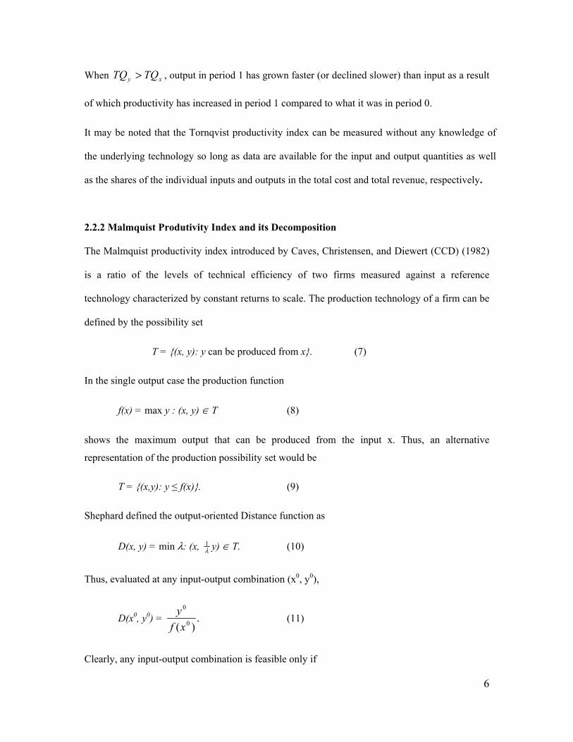
2.2.2 Malmquist Produtivity Index and its Decomposition

The Malmquist productivity index introduced by Caves, Christensen, and Diewert (CCD) (1982)

is a ratio of the levels of technical efficiency of two firms measured against a reference

technology characterized by constant returns to scale. The production technology of a firm can be

defined by the possibility set

T = {(x, y): y can be produced from x}. (7)

In the single output case the production function

f(x) = max y : (x, y) ∈ T (8)

shows the maximum output that can be produced from the input x. Thus, an alternative

representation of the production possibility set would be

T = {(x,y): y ≤ f(x)}. (9)

Shephard defined the output-oriented Distance function as

D(x, y) = min λ: (x, λ1 y) ∈ T. (10)

Thus, evaluated at any input-output combination (x0, y0),

D(x0, y0) = .)( 0

0

xfy

(11)

Clearly, any input-output combination is feasible only if

7

D(x,y) ≤ 1. (12)

Hence, the production possibility set can also be represented as

T = {(x,y): D(x,y) ≤ 1}. (13)

Farrell (1957) defined the technical efficiency of a firm producing output y from the input bundle

x as

TE(x,y) = φ1 (14)

where *φ = max .),(: Tyx ∈φφ Clearly, the output-oriented Shepard Distance function is the

same as the Farrell measure of output-oriented technical efficiency.

If we assume constant returns to scale, for any ,0≥k

.),(),( TkykxTyx ∈⇒∈ (15)

With reference to a CRS production possibility set TC, we can define the CRS production

function as R(x) = max y: (x,y) ∈TC. In this case, the CRS distance function is

.)(

),(xR

yyxDC = (16)

Note that an implication of CRS is that R(x) is homogeneous of degree one. In the single input

case,

R(x) = ax, where, a= R(1). (17)

Returning to the 1-input, 1-output case of productivity comparison between the two firms 0 and

1with input-output combinations (x0, y0) and (x1,y1),respectively, the productivity index of firm 1

relative to firm 0 is

.),(),(

)(/)(/

00

11

00

11

00

11

00

11

0

11 yxD

yxDxRyxRy

axyaxy

xyxy

C

C

====ΠΠ=π (18)

8

Thus the Malmquist productivity index is the ratio of the Distance function evaluated at two

different input output bundles.

For the more general multi-output, multi-input case, the Malmquist productivity index for

(x1, y1) with (x0, y0) as the base is

M(x1, y1; x0, y0) = .),(),(

00

11

yxDyxD

C

C

(19)

Suppose that the two input-output bundles relate to the same firm but from two different time

periods, period 0 and period 1. In that case the Malmquist index above shows how the total factor

productivity of the firm has changed from period 0 to period 1. Typically, there will be technical

change over time. In that case, there would be two different production technologies and,

correspondingly, two different Distance functions for the two different time periods. Suppose that

),( yxDCt is the CRS Distance function evaluated at the input-output bundle (x, y) in period t

(t=1, 2). We would then have two alternative measures of the Malmquist productivity index

M(x1, y1; x0, y0) = ),(),(

000

110

yxDyxD

C

C

(20a)

and

M(x1, y1; x0, y0) = .),(),(

001

111

yxDyxD

C

C

(20b)

Except in the trivial case of one output and one input, the two alternative measures will be

different. The standard practice in the literature is to take a geometric mean of the two measures.

Thus,

M(x1, y1; x0, y0) = .),(),(.

),(),( 2

1

001

111

000

110

yxDyxD

yxDyxD

C

C

C

C

(21)

9

Färe, Grosskopf, Lindgren, and Roos (FGLR) (1992) decomposed this Malmquist productivity

index as

M(x1, y1; x0, y0) = .),(),(.

),(),(

),(),( 2

1

110

111

000

001

000

111

yxDyxD

yxDyxD

yxDyxD

C

C

C

C

C

C

(22)

When the true production technology does exhibit constant returns to scale the CRS Distance

function is, in deed, a measure of the technical efficiency of a firm. Thus, the first factor in the

FGLR decomposition shows the change in technical efficiency between the two periods and can

be characterized as a “catch up” factor. A value of this factor greater than 1 implies an

improvement in efficiency and contributes to productivity growth. Each of the two ratios inside

the square brackets in the second factor is a measure of the shift in the production frontier

evaluated at the two different input bundles. Being the geometric mean of the two, the second

factor is a measure of the autonomous shift in the production frontier and represents technical

change. Again, a value of this factor in excess of 1 implies an outward shift in the frontier and

implies technical progress.

Färe, Grosskopf, Norris, and Zhang (FGNZ)(1994) offered the following extended decomposition

for the case of variable returns to scale (VRS):

M(x1, y1; x0, y0) = .

),(),(

),(),(

),(),(

.),(),(

),(),(

000

000

111

111

110

111

000

001

000

111

21

yxDyxDyxDyxD

yxDyxD

yxDyxD

yxDyxD

C

C

C

C

C

C

(23)

In this extended decomposition, the first term measures technical efficiency change. The second

and the last terms are interpreted as technical change and scale efficiency change, respectively.

As shown by Ray and Desli (RD) (1997), the Malmquist index is correctly measured by

the ratios of CRS Distance functions even when the technology does not exhibit CRS everywhere.

But in that case the FGNZ decomposition is inappropriate.2 Specifically, the last two factors

would not represent change in technical efficiency and shift in the frontier, respectively, unless

CRS holds.

10

It may be noted, however, that as shown by Banker, Charnes, and Cooper (BCC) the CRS

Distance function can be split up into two factors as

.),(),().,(),(

=

yxDyxDyxDyxD

CC (24)

The first term on the right hand side is the VRS Distance function correctly measuring technical

efficiency in the absence of CRS while the second term measures the scale efficiency of the

observed input-output bundle.

RD pointed out that the FGNZ’s second factor captures the shift in the hypothetical CRS frontier

and does not correctly measure technical change when CRS does not hold. They proposed the

alternative decomposition:

M(x1, y1; x0, y0) = .

),(),(

),(),(

),(),(),(),(

),(),(

.),(),(

),(),(

21

21

001

001

111

111

000

000

110

110

110

111

000

001

000

111

yxDyxDyxDyxD

yxDyxDyxDyxD

yxDyxD

yxDyxD

yxDyxD

C

C

C

C

(25)

In both the FGNZ and the RD decomposition the efficiency change factor is the same. RD’s

second factor correctly measures technical change as the geometric mean of the shift in the VRS

frontier at the two observed input-output bundles. The last factor can be described as a scale

change factor. It is more like a residual and is not easily interpreted. Another point to note is that

because they involve evaluating the Distance functions for the input-output bundles from one

period against the technology from the other period, in empirical applications they may not

always be estimable.

2.2.3 The Nonparametric Methodology

2 See Lovell (2003) for a detailed discussion of this issue.

11

Suppose that we have the input-output data for N firms observed over two different time

periods. Let ),...,,( 21tmj

tj

tj

tj yyyy = be the output bundle and ),...,,( 21

tnj

tj

tj

tj xxxx = the input

bundle for firm j (j = 1,2,…,N) in period t (t =0, 1). As explained before, the free disposal convex

hull of the input-output vectors observed in that period approximate production possibility set

exhibiting variable returns to scale in period t (Tt). Correspondingly, the pseudo production

possibility set (TCt) showing globally constant returns is the free disposal conical hull of these

points. In principle, one can evaluate the distance function at a specific input-output bundle (x, y)

with reference to any arbitrary production possibility set. We may describe the distance function

as the same-period distance function, if one uses the Tt (or TCt) to evaluate the distance function at

an input-output combination observed in period t. On the other hand, if the distance function

based on the technology from one period is evaluated at an input-output bundle from another

period, it can be described as a cross period distance function. As noted before, the (Shephard)

distance function is the same as the Farrell measure of technical efficiency and can, therefore, be

obtained straightaway from the optimal solution of the appropriate BCC or CCR DEA problem.

In particular, the same period (VRS) distance function is

*

1),(k

tk

tk

t yxDφ

= (26)

where φφ max* =k

s.t. ∑=

≥N

j

tk

tjj yy

1;φλ

∑=

≤N

j

tk

tjj xx

1;λ (27)

∑=

=N

jj

1;1λ ).,...,2,1(;0 Njj =≥λ

This, obviously, is the standard BCC model.

For the cross period (VRS) distance function Ds(xkt, yk

t) , one needs to solve the BCCproblem

max δ

s. t. ∑=

≥N

j

tk

sjj yy

1;φλ

12

∑=

≤N

j

tk

sjj xx

1;λ (28)

∑=

=N

jj

1;1λ ).,...,2,1(;0 Njj =≥λ

This, it may be noted, is quite different from the usual BCC model. While the input-output

quantities of firm k observed in period t appear on the right hand sides of the inequality

constraints, they do not appear on the left hand sides of these constraints. An implication of this

feature of the problem is that, unlike the BCC problem, it may not have a feasible solution. This

will be true if the quantity of any individual input of firm k in period t is smaller than the smallest

quantity of the corresponding input across all firms in period s.

For the cross period (CRS) distance function DCs(xk

t, ykt) one solves the problem above

without the constraint that the λj s have to add up to unity. Note that in the case of CRS, the DEA

problem will always have a feasible solution.

3. Literature review

Bhattacharyya et al (1997) studied the impact of the limited liberalization initiated before the

deregulation of the nineties on the performance of the different categories of banks, using DEA.

Their study covered 70 banks in the period 1986-91. They constructed one grand frontier for the

entire period and measured technical efficiency of the banks under study.

The authors use advances, investments and deposits as outputs and interest expense and operating

expense as inputs. They found public sector banks had the highest efficiency among the three

categories, with foreign and private banks having much lower efficiencies. However, public

sector banks stated showing a decline in efficiency after 1987, private banks showed no change

and foreign banks showed a sharp rise in efficiency. The main results accord with the general

perception that in the nationalized era, public sector banks were successful in achieving deposit

and loan expansion. It should be noted, however, that the use of one grand frontier for the entire

period implies that technical change is not separately accounted for.

Das (1997) analyses overall efficiency- technical, allocative and scale- at PSBs. In the period

1990-96, the study found a decline in overall efficiency. This occurred because there was a

decline in technical efficiency, both pure and scale, which was not offset by an improvement in

13

allocative efficiency. The study, however, pointed out that the deterioration in technical

efficiency was mainly on account of four nationalised banks.

In a study that covers a more recent period, Das (1999) compares performance among public

sector banks for three years in the post-reform period, 1992, 1995 and 1998. He finds a certain

convergence in performance. He also notes that while there is a welcome increase in emphasis on

non-interest income, banks have tended to show risk-averse behaviour by opting for risk-free

investments over risky loans.

Sarkar, Sarkar and Bhaumik (1998) compared performance across the three categories of banks,

public, private and foreign, in India, using two measures of profitability, return on assets and

operating profit ratio, and four efficiency measures, net interest margin, operating profit to staff

expense, operating cost ratio and staff expense ratio (all ratios except operating profit to staff

expense having average total assets in the denominator). The authors attempted these

comparisons after controlling for a variety of non-ownership factors that might impact on

performance: asset size, the proportion of investment in government securities, the proportion of

directed credit, the proportion of rural and semi-urban branches, and the proportion of non-

interest income to total income.

They found that, in the comparison between private banks and PSBs, there was only a weak

ownership effect. Traded private banks were superior to PSBs with respect to profitability

measures but not with respect to efficiency measures. Non-trade private banks did not

significantly differ from PSBs in respect of either profitability or efficiency.

There was, however, a strong ownership effect between foreign banks and private banks, with the

former outperforming the latter with respect to all indicators. The authors conclude that the

results showed that private enterprises may not be unambiguously superior to public enterprises

in a developing economy. They ascribe the particular ordering that they found- foreign, traded

private, non-traded private and public- to the link between performance and the market for

corporate control. The stronger the link, they suggest, the better the performance. We believe,

however, that this study suffers from an important shortcoming. It is confined to just two years

after financial sector reform, 1993-94 and 1994-95. In one of these, 1993-94, the performance of

PSBs was adversely impacted by the introduction of new prudential and accounting norms. Any

comparison using the performance parameters for these two years is unlikely to fully reflect

14

differences in managerial performance. We address this shortcoming in our own analysis by

using a much longer period for comparison.

Ram Mohan (2002) found a trend towards convergence in performance among the three

categories of banks- public, private and foreign- using financial measures of performance. Ram

Mohan (2003) found that this result was reinforced by a comparison of returns to stocks in the

three categories- the evidence was that returns to public sector bank stocks were not significantly

different from returns to private sector bank stocks.

4. The Empirical Analysis

As mentioned earlier, we use two measures for our comparisons: Tornqvist total factor

productivity growth (TFP) and Malmquist TFP growth

For the comparison based on quantities, it is necessary to be clear about what we should regard as

outputs and inputs. As Mukherjee et al (2001) point out, there is no consensus on what best

measures these in the case of banks. In the production approach, banks produce loans and deposit

account services, using labor and capital as inputs. (Berger and Humphrey (1992) refer to this as

the ‘value-added approach’.) The number of accounts measures outputs and production costs

include only operating costs (although, in the literature, there are instances of the dollar value of

accounts being used as outputs in the production approach.)

In the intermediation approach, banks collect funds and, using labor and capital, transform these

into loans and other assets. This approach treats the dollar value of accounts as outputs and

production costs include both operating and interest costs.

As Wykoff (1992) points out, the issue of whether deposits are to be regarded as inputs or outputs

remains unresolved. If bank deposits are regarded as inputs and there are no associated outputs,

then it is not clear why depositors spend so much time and effort to travel to banks to give them

these free inputs. If deposits are outputs, then it has to be explained why their nominal prices

have been comparatively stable and even falling in real times over the years. This would imply

that banks have undertaken to make these outputs cheap- it is not clear why.

Mukerjee et al (2001), adopting the intermediation approach, use as outputs the following:

consumer loans, real estate loan, investments, total non-interest income. As inputs they use the

following: transaction deposits, non-transaction deposits, equity, labor and capital (measured by

non-labor, non-interest expense).

15

In the Indian context, we need to be clear about which approach is most appropriate. Using

deposits and loans as outputs would have been appropriate in the nationalized era when

maximizing these was indeed the objective of bank but they are, perhaps, less appropriate in the

reforms era. Banks are not simply maximizing deposits and loans, they are in the business of

maximizing profit. Maximizing loans and deposits may not necessarily be consistent with profit

maximization because the quality of bank loans, not just quantity, is crucial to profit.

Keeping in mind the above considerations, we compute Tornqvist and Malmquist total factor

productivity growth for the three categories of banks, public sector, domestic private sector and

foreign, using as outputs the following: loan income, investment income and non-interest income.

For inputs, we use: interest cost and operating cost (which includes labor and non-labor, non-

interest costs). Thus, both outputs and inputs will comprise flow items. Both inputs and outputs

are deflated by the price index. For comparison, we also compute Tornqvist TFP growth using

(amounts of) loans and investments and other income as outputs and deposits (rather than interest

expense) and operating costs as inputs.

The period covered is 1992-2000. For the Tornqvist TFP computation, we have data for

27 PSBs, 21 old private sector banks and 14 foreign banks (Where data for some banks

was available for most of the period, data for the relevant years was included in the

computation.) For the Malmquist TFP computation, we have a slightly smaller sample of

banks: 27 PSBs, 20 private sector banks and 11 foreign banks.3

4. Results

3 The reason that the sample is slightly different in the latter case is that, for the latter, we used a balanced panel for

computing the Malmquist productivity indexes.

16

4.1 Tornqvist total factor productivity growth

Table 2 presents the results for Tornqvist TFP growth in the three categories of banks- public

sector, domestic private sector and foreign banks-, using interest income, investment income and

other income as outputs and interest cost and operating cost as inputs. Table 3 compares growth

in the three categories, while table 4 provides the average frequency distribution of the TFP

growth over the period for the different categories.

Table 2: Comparison of Tornqvist TFP growth, using income as outputs

Year Growth rate-PSU(%) Growth rate-Pvt(%)

Growth rate-Foreign(%)

1992-93 -8.16 -3.63 1.901993-94 5.69 6.76 11.271994-95 5.79 4.89 - 1.901995-96 -0.16 -1.71 -20.191996-97 2.22 -0.70 1.001997-98 1.58 0.99 -2.621998-99 -3.00 -8.78 -14.241999-00 2.99 7.18 4.06Average 0.77 0.49 -3.07

Note: figures in the three columns represent the average for each category for a given year.

Table 3: Comparison of Tornqvist TFP growth in Indian banking

Sample size Mean growthrate

t-statistic (Public and pvt)

t-statistic (Publicand foreign)

Public sector 27 0.77% 0.11 0.94Private sector 21 0.49% (0.46) (0.18)Foreign 14 -3.07%Note: 1. Means are for the period 1991-92 to 1999-00 2. Figures in brackets indicate levels of significance

Table 4: Average distribution of banks in Tornqvist TFP growth range

17

PSB % of total Private % of total Foreign % of total<-20% 0 0.00% 0 0.00% 2 11.76%-20-15% 0.75 2.78% 0.5 2.38% 0.75 4.41%-15-0% 10.125 37.50% 9.875 47.02% 5.75 33.82% 0-10% 14.25 52.78% 7.5 35.71% 3.875 22.79%10-20% 1.75 6.48% 2.75 13.10% 3.375 19.85%>20% 0.125 0.46% 0.375 1.79% 1.25 7.35%

It can be seen from table 3 that there is no significant difference in Tornqvist TFP growth either

between public and private sector banks or between public sector and foreign banks. We

computed but do not report here the results for private sector banks after including new private

sector banks for the limited period for which the latter have been in existence. The comparison

remains unaffected although the growth rate for private sector banks rises slightly with the

inclusion of new banks.

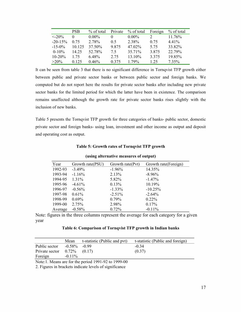
Table 5 presents the Tornqvist TFP growth for three categories of banks- public sector, domestic

private sector and foreign banks- using loan, investment and other income as output and deposit

and operating cost as output.

Table 5: Growth rates of Tornqvist TFP growth

(using alternative measures of output)

Year Growth rate(PSU) Growth rate(Pvt) Growth rate(Foreign)1992-93 -3.49% -1.96% 14.35%1993-94 -1.16% 2.13% -8.96%1994-95 1.31% 5.82% -1.47%1995-96 -4.61% 0.13% 10.19%1996-97 -0.56% -1.33% -10.25%1997-98 0.61% -2.51% -2.64%1998-99 0.69% 0.79% 0.22%1999-00 2.75% 2.98% 0.17%Average -0.58% 0.72% -0.11%

Note: figures in the three columns represent the average for each category for a givenyear

Table 6: Comparison of Tornqvist TFP growth in Indian banks

Mean t-statistic (Public and pvt) t-statistic (Public and foreign)Public sector -0.58% -0.99 -0.34Private sector 0.72% (0.17) (0.37)Foreign -0.11%Note:1. Means are for the period 1991-92 to 1999-002. Figures in brackets indicate levels of significance

18

Once again, as can be seen from table 6, there is no significant difference in Tornqvist TFP

growth either between public and private sector banks or between public sector and foreign

banks. This also applies when the results for private sector banks are computed after including

new private sector banks. However, it will be noticed that the public sector shows the highest

growth in TFP among the three categories in the first approach and the lowest growth in the

second approach. This accords with the fact that, in the period since deregulation, PSBs’ focus

has been on asset quality rather than asset growth. Not surprisingly, TFP growth turns out to be

low when we use loans and investments as output. However, PSBs have, as we have seen,

managed to improve profitability, which means they have seen growth in revenues relative to

costs. This shows up in a positive TFP growth when loan income and investment income are

treated as output.

4.2 Malmquist TFP growth

Table 7 below gives the results of Malmquist TFP growth for the bank categories for

each year. Table 8 compares growth among the categories, while Table 9 provides the

frequency distribution. As can be seen from Table 10, PSBs are seen to do better than

private banks at a 10 per cent level of significance and worse than foreign banks at an 8

per cent level of significance. 4

Table 7 Year- wise averages for Malmquist TFP growth for bank categories

Growth(PSB) Growth(Pvt) Growth(Foreign)1992-93 -5.14% -6.59% 1.97%1993-94 -1.02% 3.26% 13.65%1994-95 -1.05% 2.86% 4.59%1995-96 3.92% 0.83% 14.06%1996-97 5.20% -0.25% -13.03%1997-98 -0.35% -7.13% -1.80%1998-99 2.71% -5.99% 15.97%1999-00 2.10% -1.11% 38.37%Average 0.80% -1.76% 9.22%

Table 8 Comparison of Malmquist TFP growth in Indian banks

4 The foreign bank category’s average productivity growth rate has been boosted by an unusually high increase inproductivity at one bank in 2000. We would, therefore, interpret this finding with caution.

19

Sample size Mean growth rate t-statistic (Publicand pvt)

t-statistic (Public and foreign)

Public sector 27 0.80% 1.35(0.1)

Private sector 20 -1.76%Foreign 11 9.22% -1.45

(0.08)Note:1. Means are for the period 1991-92 to 1999-00 2. Figures in brackets indicate levels of significance

Table 9 Distribution of banks by Malmquist TFP growth ranges

PSB % of total Private % of total Foreign % of total<-20% 0.5 1.85% 1.5 7.50% 2 18.18%

-20-15% 0.625 2.31% 1.375 6.88% 0.75 6.82%-15-0% 12.75 47.22% 8.875 44.38% 2.625 23.86%0-10% 9 33.33% 5 25.00% 1.75 15.91%

10-20% 2.75 10.19% 2 10.00% 1 9.09%>20% 1.375 5.09% 1.25 6.25% 2.875 26.14%

As explained above, one can extract the contribution of change in technical efficiency

over time from the Malmquist productivity index. In Table 10 below the contributions of

technical efficiency change and the residual factor consisting of technical change and

scale change in the Malmquist productivity index are separately reported. One problem of

the technical efficiency change factor is that when a firm is already at a high level of

efficiency, there is little room for further improvement and its rate of increase in technical

efficiency will be low. To address this problem, we also report the average levels of

technical efficiency for the different ownership categories.

Table 10. Group-wise Average Levels and Annual Rates of Change in Technical Efficiency

Public SectorBanks

Private SectorBanks

ForeignBanks

Technical Efficiency Change -0.075% -3.416% 0.331%

Level of Technical Efficiency 0.8787 0.6473 0.9403

Contribution of Technical and ScaleChange

1.5596% 1.8914% 8.9819%

20

Only foreign banks show an improvement in technical efficiency while both public and priva5te

firms show a decline – marginal in the case of public sector banks and quite pronounced for

private banks. Also the average level of technical efficiency is significantly higher for foreign

banks compared to the PSBs. At the same time, PSBs operated at a higher level of efficiency than

the private banks.

4.4 Summary of comparisons between bank categories

We are now in a position to summarize the results obtained in the comparison of the three

categories of banks using both financial measures and input-output quantities. These are

summarized in Table 11 below.5

Table 11 Summary of comparison of performance in bank categories

Measure/comparison Result1. Tornqvist TFP growthi. PSBs and old private sector banks No differenceii. PSBs and foreign banks No difference

2. Malmquist TFP growthi. PSBs and old private sector banks PSB better at 10 per cent level of significanceii. PSBs and foreign banks Foreign better at 8 per cent level

Out of a total of four comparisons we have made, there are no differences in two cases, PSBs do

better in one, and foreign banks in one. To put it differently, PSBs are seen to be at a

disadvantage in only one out of four comparisons. It is difficult, therefore, to sustain the

proposition that productivity is lower in public sector banks relative to their peers in the private

sector.

5 Annual average rates of productivity change (Malmquist as well as Tornqvist) along with levels oftechnical efficiency for individual banks are reported in an appendix Table for the interested reader.

21

5. Concluding remarks

We have compared efficiency and productivity of PSBs relative to private sector banks, both

domestic and foreign. This comparison is attempted over a nine year period (1992-00), out of

which eight years belong to what might be called the post-deregulation period, if we use the

generally accepted year of 1992-93 as the cut off date for the big push in bank deregulation. Our

results are interesting given the general belief that deregulation would expose the inefficiencies

inherent in government ownership and result in a huge gap between private banks and PSBs. This

has not happened. We are unable to uncover any significant differences in productivity growth

between the public and private sectors in the period under study. The findings of this study thus

reinforce those of Ram Mohan (2002) and Ram Mohan (2003) that failed to uncover any

significant differences between PSBs and other categories of banks using financial measures of

performance or returns to stocks.

It is possible to speculate on why this is so, that is, why the expectation of superior private

performance that one finds in both the theoretical and empirical literature on privatization has not

been borne out in the Indian banking sector. One explanation could be that there has been a

change in orientation in PSBs from social objectives towards an accent on profitability, especially

given that some of these have come to be listed on the exchanges and have private investors.

Another is that PSBs enjoy a huge advantage in terms of scale of operations over private sector

banks and these advantages offset any inefficiency that could be ascribed to government

ownership.

Those who advocate privatization of PSBs could contend that a transfer to private control could

improve productivity at PSBs even further. But that is quite different from arguing that there is a

performance differential between PSBs and their private sector counterparts today that justifies

privatization.

References

Banker, R.D., A. Charnes, and W.W. Cooper (1984), “Some Models for Estimating Technicaland Scale Inefficiencies in Data Envelopment Analysis,” Management Science, 30:9 (September),1078-92.

22

Berger Allen N and Humphrey David B. 1992.Measurement and efficiency issues incommercial banking in: Z.Griliches (Ed), Output Measurement in Services Sector. University ofChicago Press,Chicago, IL, 245-279

Bhattacharyya Arunava,. Lovell C.A.K. and Sahay Pankaj, 1997. The impact of liberalization onthe productive efficiency of Indian commercial banks. European Journal of OperationalResearch 98, 332-345

Caves, D.W., Christensen, L.R., Diewert, W.E., (1982). The economic theory of index numbersand the measurement of input, output and productivity, Econometrica 50, 1393-1413.

Das, Abhiman (1997). Technical, Allocative and Scale Efficiency of Public Sector Banks inIndia, RBI Ocasional Papers, 18, June-September.

Das, Abhiman (1999) Profitability of Public sector Banks: A Decomposition Model; RBIOcasional Papers, 20, 1.

Fare, R., S. Grosskopf, B. Lindgren and P. Roos (1992). Productivity changes in Swedishpharmacies 1980-89: A nonparametric Malmquist approach. Journal of Productivity Analysis, 3,85-101.

Fare, R., S. Grosskopf, Norris, and P. Zhang (1994). Productivity growth, technical progress,and efficiency changes in industrialized Countries. American Economic Review, 84:1, 66-83.

Lovell, C.A.K. (2003). The Decomposition of Malmquist Productivity Indexes. Journal ofProductivity Analysis, Vol 20, 437-458.

Mukherjee Kankana, Ray Subhash C and Miller Stephen M., 2001. Productivity growth in largeUS commercial banks: The initial post-deregulation experience. Journal of Banking and Finance,25, 913-939.

Ram Mohan, T. T. (2002) ‘Deregulation and performance of public sector banks’,Economic and Political Weekly 37 (5): 393-397.

Ram Mohan, T. T. (2003) ‘Long-run performance of public and private sector bank

stocks’, Economic and Political Weekly 38 (8): 785-788.

Ray, S. C. And E. Desli, (1997). Productivity growth, technical Progress, and efficiency changein industrialized countries: comment. American Economic Review, Vol 87, No.5, pp 1033-1039

Ray, S.C. (2004) Data Envelopment Analysis: Theory and Techniques for Economics andOperations Research (New York: Cambridge University Press).

Sarkar, Jayati, Sarkar, Subrata and Bhaumik, Suman K. (1998) ‘Does ownership alwaysmatter? – evidence from the Indian banking industry’, Journal of ComparativeEconomics 26: 262-81.

Wykoff Frank C., Comment on “Measurement and efficiency in banking”, in Z.Griliches (Ed),Output Measurement in Services Sector. University of Chicago Press, Chicago, IL, 279-287

23

24

Appendix

Average Annual Measures of Indexes of Productivity and Efficiency Change

Bank TEChange Malmquist TE TornquistState Bank of India 1 1.00075 1 0.970703State Bank of Bikaner & Jaipur 0.98875 0.970875 0.830667 1.009767State Bank of Hyderabad 0.9785 0.989625 0.895 0.986047State Bank of Indore 1.014375 0.993625 0.749889 0.988834State Bank of Mysore 1.011375 0.97475 0.761444 0.997632State Bank of Patiala 1.00075 0.999125 0.842333 0.97631State Bank of Saurashtra 1.0235 0.966375 0.771333 0.976373State Bank of Travancore 0.983875 0.98925 0.885 1.03408Allahabad Bank 1.00025 1.055375 0.885889 1.002104Andhra Bank 0.9595 0.9655 0.792556 1.006234Bank of Baroda 0.992 1.0085 0.989556 1.011966Bank of India 1.00075 1.03625 0.974778 0.976003Bank of Maharashtra 0.982 1.03225 0.844444 0.98457Canara Bank 0.985125 1.0045 0.985889 0.995877Central Bank of India 0.990625 1.033625 0.894 0.98965Corporation Bank 0.950875 0.944375 0.907889 1.043432Dena Bank 0.9655 0.963875 0.831556 1.022248Indian Bank 1.02475 1.074 0.937778 0.961052Indian Overseas Bank 1.00925 1.05 0.908667 0.984308Oriental Bank of Commerce 0.965125 0.95025 0.927444 1.033885Punjab & Sind Bank 0.991625 1.01725 0.773667 0.995943Punjab National Bank 1.007125 0.982125 0.993556 1.000218Syndicate Bank 0.9885 1.029 0.856111 1.006196UCO Bank 0.99675 1.077125 0.905444 0.994588Union Bank of India 0.99425 1.0225 0.893556 1.006812United Bank of India 0.986125 1.0485 0.916778 0.971677Vijaya Bank 1.006375 1.03575 0.769111 0.963907Public Sector 0.992505 1.007968 0.878679 0.995941Bank of Madura Ltd. 0.975125 0.978125 0.709 1.008771Bharat Overseas Bank Ltd. 1.0265 1.017875 0.571333 0.969282City Union Bank Ltd. 0.91575 0.944875 0.633556 1.001098Lord Krishna Bank Ltd. 0.905625 0.977 0.598667 1.060654Tamilnad Mercantile Bank Ltd. 0.955375 0.9965 0.681 1.017618The Bank of Rajasthan Ltd.. 1.036375 0.971375 0.628889 1.020387The Benares State Bank Ltd. 0.939 0.989125 0.467111 1.013591The Catholic Syrian Bank Ltd. 1.000875 1.002 0.616 0.996939The Dhanalakshmi Bank Ltd. 0.90625 0.931625 0.561778 1.053675The Federal Bank Ltd. 0.97275 0.948625 0.860778 1.062209The Jammu and Kashmir Bank Ltd 1.001375 1.024 0.891444 0.980062The Karnataka Bank Ltd. 0.971875 0.97975 0.740556 1.005232The Karur Vysya Bank Ltd. 0.963625 0.961125 0.647 0.997068The Lakshmi Vilas Bank Ltd. 0.954875 0.959875 0.607556 1.005058The Nainital Bank Ltd. 0.916875 1.067875 0.363 0.973176The Nedungadi Bank Ltd. 0.989125 1.006375 0.508333 1.011317

25

The Sangli Bank Ltd. 0.986875 1.010625 0.508 0.97628The South Indian Bank Ltd. 0.981625 0.99575 0.669556 1.02149The United Western Bank ltd. 0.936 0.918 0.732667 1.000906The Vysya Bank Ltd. 0.966875 0.967125 0.950222 0.998734Private Banks 0.965138 0.982381 0.647322 1.008677ABN-AMRO Bank N.V. 0.966125 1.055375 0.966444 1.089579ANZ Grindlays Bank Ltd. 0.991375 1.110625 0.918889 0.9874Abu Dhabi Commercial Bank Ltd. 1.109125 1.08575 0.928778 0.949985American Express Bank Ltd. 1.007875 1.017 0.950333 1.144692Bank of America NT & SA 1.03525 1.190375 0.950333 1.03168Barclays Bank PLC 1 1.09925 1 1.180569Citibank N.A. 1.002375 1.09 0.985778 0.97304Credit Lyonnais 0.94125 1.042375 0.868111 1.111307Deutsche Bank AG 1.001375 1.048375 0.966 1.010692Oman International Bank S.A.O.G. 0.981625 1.121 0.808444 1.224363The Bank of Nova Scotia 1 1.1545 1 0.90401Foreign Bank 1.003307 1.092239 0.940283 1.055211

Notes: 1. TE Change, Malmquist, and Tornqvist are indexes. A value greater (less) than unity

Implies an increase (decrease) compared to the previous year.

2. TE is the level of technical efficiency.