productivity comparison and international competitiveness · include variations in the yen-dollar...
TRANSCRIPT

Journal of Applied Input-Output Analysis, Vol. 5, 1999
Productivity Comparison and International Competitiveness
By
Masahiro Kuroda*and Koji Nomura*
Abstract
This paper aims to provide an international comparison of the level of technology by industry between Japan and the United States during the period 1960-95. The methodology for the international comparison of the level of technology and the definition for the international competitiveness of industry are on the same line with our previous analysis, reported on Jorgenson, Kuroda and Nishimizu (1987), and Jorgenson and Kuroda (1990). In this paper, we tried to focus on the assessment of trends in productivity growth after the oil crisis in Japan and the U.S. We conclude that only seven industries of thirty in the Japanese industries could catch up the U.S. industries in terms of the level of productivity at the beginning of 1990s'. The productivity growth in Japan and the U.S. has revived slightly since 1980. The growth rates in the 1980s' were well below those in the 1960s'.
1. Introduction The purpose of this paper is to provide an international comparison of the level of difference in technology between the United States and Japanese industry during the period 1960-92. It is based upon the theoretical foundation for the measurement of total factor productivity at industry level. When comparing aggregate economic growth between the U.S. and Japan, it was found that the years 1960-72 saw a period of substantial economic growth in the U.S., and extremely rapid growth in Japan. Almost all of the narrowing of the gap between the two economies' levels of output during this period was due to: (1) an increase in the level of technology in Japan relative to the U.S.; and (2) the rapid growth of capital accumulation in Japan. Disaggregated analyses of the differences in the pattern of production at industry level will facilitate a better understanding of the anatomy of our findings at the macro level. The political relationship between Japan and the United States has become increasingly pre-occupied with "trade frictions" in the last few decades. These disputes over trade issues have accompanied the massive expansion of Japanese exports to the United States. Explanations for the resulting trade imbalance must include variations in the yen-dollar exchange rate, changes in the relative prices of capital and labor, and the relative growth of productivity in Japanese and U.S. industries. We will analyze the role of each of these factors in explaining the rise in
Manuscript received April 1, 1998. Revised October 16, 1999. *Keio University, Japan

2 Journal of Applied Input-Output Analysis, Vol. 5, 1999
competitiveness of Japanese industries relative to their U.S. counterparts. At the outset of our discussion, it is essential to define a measure of international competitiveness. Our measure of international competitiveness is based on the price of an industry's output in Japan relative to the price in the U.S. Japanese exports are generated by U.S. purchases from Japanese industries; while U.S. exports result from Japanese purchases from U.S. industries. The relative price of an industry's output is taken into consideration by purchasers in both countries and the rest of the world. In order to explain changes in international competitiveness, we must account for changes in the determinants of this relative price. The starting point for our analysis of the competitiveness of Japanese and U.S. industries is the yen-dollar exchange rate. This is simply the number of yen required to purchase one U.S. dollar on the foreign exchange market. Variations in the yen-dollar exchange rate are easy to document, and are often used to characterize movements in relative prices in the two countries. However, movements in relative prices of goods and services do not coincide with variations in the exchange rate. To account for changes in international competitiveness, a measure of the relative prices of specific goods and services is required. To assess the international competitiveness of industries, it is necessary to carry out price comparisons of industrial output between Japan and the United States. These comparisons have substantially some difficulties, because of various differences of industrial output even in a given industry. For example, the steel industry produces an enormous range of different steel products. The relative importance of different types of steel differs between the two countries. The composition of the output of the steel industry in each country also changes over time. These differences must be taken into account when comparing the relative prices of steel between Japan and the U.S. We have to begin with the observation of the price of the well-defined commodity between Japan and the U.S. Observed set of prices of the well-defined commodities in a specific industry could be summarized as a purchasing power parity for the industry's output. The purchasing power parity for a specific industry's output is the number of yen required to purchase an amount of that industry's output in Japan, costing one dollar in the United States. The dimensions of purchasing power parities are the same as the yen-dollar exchange rate: namely yen per dollar. However, the purchasing power parities reflect the relative prices of the goods and services rather than currencies. The most familiar application of the notion of purchasing power parity is to construct the relative prices of same aggregates as the gross domestic product. This application has been the focus of the landmark studies by Kravis, Heston, and Summers (1978). As a consequence of their research, it is possible to compare the relative prices of gross domestic product for a wide range of countries, including Japan and the United States. Kravis, Heston, and Summers have based their purchasing power parities for gross domestic product on relative prices in 153 commodity groups. The OECD (1988 and 1993) followed the same line of the work, publishing the PPP index among OECD countries. In particular, the PPP indices for Japan and the U.S. are available in the expenditure items that are classified by 163 consumption items and 29 investment items. The index represents Japanese prices, relatively evaluated by unity of the U.S. prices, and volumes of the expenditures in both countries. These are the basic sources for our PPP index by commodity. Finally, we try to estimate purchasing power parities for thirty industries in Japan and the U.S.

Productivity Comparison and International Competitiveness 3
during the period 1960-92, where industry classification for our international comparison is shown in Table 1. These can be observed as the relative prices of the outputs of each industry in the two countries, which are evaluated for a certain amount of quantity. We divide the relative price of each industry's output by the yen-dollar exchange rate in order to translate purchasing power parities into relative prices in terms of dollars. We find it convenient to employ relative prices in dollars, as measures of international competitiveness. Variations in the exchange rate are reflected in the relative prices of outputs for all industries. We will explain our process for the estimation of PPP index by commodities in Section 3. To account for changes in international competitiveness between Japanese and U.S. industries, we have compiled purchasing power parities for the inputs into each industry, which are also shown in Section 3. We have disaggregated inputs among capital and labor services, which are primary factors of production; and energy and other intermediate goods, which are produced by one industry and consumed by others. We can translate purchasing power parities for inputs into relative prices in dollars by dividing by the yen-dollar exchange rate. Our final step in accounting for international competitiveness between Japanese and U.S. industries is to measure the relative levels of productivity for all thirty industries. For this purpose we employ a model of production for each industry. This model enables us to express the price of output in each country as a function of the prices of inputs and the level of productivity in that country. We can account for the relative prices of output between Japan and the U. S. by allowing input prices and levels of productivity to differ between countries. We have compiled data on relative productivity levels in Japan and the U.S. for the period 1960-95. The methodology for our study was devised by Jorgenson and Nishimizu (1978). They provided a theoretical framework for productivity comparisons, based on a bilateral production function at the aggregate level. They employed this framework in comparing aggregate output, input, and productivity for Japan and the U.S. This methodology was extended to the industry level by Jorgenson and Nishimizu (1981) and employed in international comparisons of Japanese and U.S. industries. The industry-level methodology introduced models of production for individual industries, based on bilateral production functions for each industry. We will summarize our method briefly in Section 2. We present comparisons of productivity levels between the U.S. and Japan by industry in Section 4. We can construct our taxonomy of the Japanese and the U.S. industries from the viewpoint of the historical patterns of productivity growth in both countries. Finally, we try to summarize changes in international competitiveness between Japanese and U.S. industries during the period 1960-92 at the aggregated level in Section 5. We try to refer to the theoretical value of the exchange rate between yen and dollar, where industry's output price adjusted by the exchange rate were equalized in both countries.

4 Journal of Applied Input-Output Analysis, Vol. 5, 1999
Common 164Industry Commodity
1 1 agric. 1 agric. 1-14 2 2 coal mining 3 coal mining 183 3 other mining 2 metal mining 15-17
4 oil and gas extract. 19 5 non-metallic mining
4 4 construct. 6 construct. 117-124 5 5 foods 7 foods 20-35
8 tobacco 6 6 textile 9 textiles 36-377 7 apparel 10 apparels 38-408 8 woods prod. 11 woods 41-43 9 9 furniture 12 furniture 44
10 10 paper & pulp 13 paper 45-48 11 11 printing 14 printing 49-5012 12 chemical 15 chemical 51-6013 13 petroleum 16 petroleum 61
14 coal prod. 14 16 leather 18 leather 65-6615 17 stone & clay 19 stone 67-7316 18 iron & steel 20 prim.metal 74-78
19 non-ferrous 17 20 metal prod. 21 fab.metal 79-80 18 21 machinery 22 machinery 81-86 19 22 elec. mach. 23 elec.mach. 87-100 20 23 motor vehicle 24 motor vehicle 10121 24 other transp.mach. 25 other trasp. eqpt. 102-105 22 25 precision inst. 26 precision instr. 106-109 23 26 other misc.manuf. 27 miscc. manuf. 62-64
15 rubber prod. 17 rubber and misc. pla 110-11624 27 railway 28 transportation 134-139
28 road trans. 29 water trans. 30 air trans 31 storage
25 32 communication 29 communication 140-141 26 33 electricity 30 electiric utilities 12527 34 gas supply 31 gas utilities 12628 36 trade 32 trade 129-13029 37 finance 33 finance and real esta 131-133
38 real estate 30 35 water supply 34 service 127-128
39 education 35 gov.service 142-164 40 research 41 medical serv. 42 other serv. 43 gov. service
Table 1:Industry Classification for our International ComparisonJapanese U.S.Industry Industry

Productivity Comparison and International Competitiveness 5
2. Theoretical Framework Our methodology is based on the economic theory of production. The point of departure for this theory is a production function for each industry, giving output as a function of inputs; a dummy variable equal to zero for the United States and one for Japan, and a time factor. We consider production under constant returns to scale, so that a proportional change in all inputs results in a proportional change in output. In analyzing differences in industrial production patterns between the two countries, we combine the production function with necessary conditions for producer equilibrium. We express the condition as that of equalities between share of input in the value of output of each industry, and the elasticity of output with respect to that input in the industry. The elasticity depends on input level, the dummy variable for each country, and time. Under constant return to scale, the sum of the elasticity (with respect to all inputs) is equal to unity, so that the value shares also sum to unity. We begin with a model of production that provides the analytical framework for international comparison of differences in outputs, inputs, and levels of technology. Our methodology is based on a specific form of production function, giving output as a function of inputs, a country's dummy variable, and time factor for each industry: To represent our bilateral models of production we require the following notation: q j : price of the output of the j-th industry,
p p p pKj
Lj
Ej
Mj
, , , : prices of capital, labor, energy, and other intermediate inputs in the j-th industry, v v v vK
jLj
Ej
Mj
, , , : value shares of capital, labor, energy and other intermediate inputs in the j-th industry, v j : the column vector of value shares of input in the j-th industry,
ln p j : the column vector of logarithms of input prices of the j-th industry, T : time trend as an index of technology , D : dummy variable D, equal to one for Japan and zero for the U.S. to represent differences in technology between the two countries. Under competitive conditions, we can represent technology by a price function that is dual to the production function, relating each industry's output to the corresponding inputs, and the level and differences in technology between the two countries:
For each industry the price of output is a transcendental or, more specifically, exponential function of the logarithms of the input prices. In this translog representation the scalars --- α t
j ,α dj , βtt
j , βddj --- the vectors --- α j , βt
j , βdj --- and
the matrices, B j , are constant parameters that differ among industries. These parameters reflect differences in technology among industries. Within each industry
ln ln ln ln ln ln
, ( , , , ).
' ' ' 'q p T D p B p p T p D
T TD D j J
j j jtj
dj j j j j
tj j
dj
ttj
tdj
ddj
= + + + + +
+ + + =
α α α β β
β β β
12
12
12
1 22 2 K (1)

6 Journal of Applied Input-Output Analysis, Vol. 5, 1999
differences in technology among time periods are represented by time as an index of technology. Differences in technology between Japan and the U.S. are represented by a dummy variable, equal to one for Japan and zero for the U.S. In analyzing differences in each industry's production patterns, we combine the price function with demand functions for inputs. We can express the function as equality between share of input in the value of the output of the industry, and the elasticity of the output price with respect to the price of that input. The elasticity depends on input prices, dummy variables for each country, and time as an index of technology. The sum of the elasticity is equal to unity, so that the value shares also sum to unity. For each industry the value shares are equal to the logarithmic derivatives of the price function, with respect to logarithms of the input prices:
v B p T D j Jj j j jtj
dj= + + + =α β βln , ( , , , ).1 2 K (2)
We can define rates of productivity growth, say vTj , as the negative of rates of
growth of the price of output with respect to time, holding the input prices constant: − = + + + =v p T D j JT
jtj
tj j
ttj
tdjα β β β' ln , ( , , , ).1 2 K (3)
Similarly, we can define differences in technology between Japan and the U.S., say vD
j , as the negative of rates of growth of the price of output with respect to the dummy variable, holding the input prices constant:
− = + + + =v p T D j JDj
dj
dj j
tdj
ddjα β β β' ln , ( , , , ) .1 2 K (4)
The price of output, the prices of inputs, and the value shares for all four inputs are observable for each industry during the period 1960-92 in both countries. The rates of productivity growth are not directly observable. Average rates of productivity growth between two points of time, say t and t-1, can be expressed as the difference between a weighted average of growth rates of input prices, and the growth rates of the price of output for each industry:
− = − − − − − =v q t q t v p t p t j JTj j j j j jln ( ) ln ( ) [ln ( ) ln ( )], ( , , , ),'1 1 1 2 K (5)
where the average rates of technical change are:
v v t v t j JTj
Tj
Tj= + − =1
21 1 2[ ( ) ( )], ( , , , ),K (6)
and the weights are given by the average value shares:
v v t v t j Jj j j= + − =12
1 1 2[ ( ) ( )], ( , , , ).K (7)
We refer to the index numbers (5) as translog price indices of the rates of productivity growth. Similarly, differences in productivity vD
j are not directly observable. However, the average of these differences for Japan and the U.S. can be expressed as a weighted average of differences between the logarithms of the input prices, less the difference between logarithms of the output price:
− = − − −=
v q JAPAN q U S v p JAPAN p U Sj J
Dj j j j j jln ( ) ln ( . .) [ln ( ) ln ( . .)],
( , , , ),
'
1 2 K (8)
where the average differences in productivity are:
Productivity Comparison and International Competitiveness 7
v v JAPAN v U S j JDj
Dj
Dj= + =1
21 2[ ( ) ( . .)], ( , , , ),K (9)
and the weights are given by the average value shares:
v v JAPAN v U S j Jj j j= + =12
1 2[ ( ) ( . .)], ( , , , ).K (10)
We refer to the index numbers (9) as translog price indices of differences in productivity. In our bilateral models of production, the capital, labor, energy and other intermediate input prices are defined as aggregate indices that depend on the prices of individual capital inputs, labor inputs, energy inputs and other intermediate inputs, respectively. The product of price and quantity indices must equal the value of all the components of each aggregate. Quantity indices of inputs are defined as ratios of the compensation of input to the corresponding price index. In international comparisons the price indices should represent purchasing power parities between the yen and the dollar. For example, the price index for labor input represents the Japanese price in yen for labor input costing one dollar in the U.S. Our methodology for estimating purchasing power parities is based on linking time series data sets with prices in Japan and the U.S. Suppose that we observe the price of the output of the j-th industry in Japan and the U.S., say q JAPANj ( , )0 and q U Sj ( . ., )0 , in the base period, where these prices are evaluated in terms of yen and dollars, respectively. We can define the purchasing power parity for the output of the j-th industry in the base period, say PPP j ( )0 , as follows:
PPP q JAPANq U S
j Jjj
j( ) ( , )( . . , )
, ( , , , ).0 00
1 2= = K (11)
The purchasing power parity gives the number of yen required in Japan to purchase an amount of the output of the j-th industry costing one dollar n the U.S. in the base period. To estimate purchasing power parities for outputs in Japan and the U.S. for every year, we first construct a time series of prices for the output of each industry in both countries in domestic currency. To obtain price indices for industry outputs in the U.S., we normalize the price index for each industry, say q U S tj ( . ., ) , at unity in the base period. We normalize the corresponding price index for Japan, say q JAPAN tj ( , ) , at the purchasing power parity in the base period. We obtain estimates
of purchasing power parities for every year, say PPP tj ( ) , from these price indices and the purchasing power parity for the base period from the equation:
PPP t PPP q JAPAN t q U Sq JAPAN q U S t
j Jj jj j
j j( ) ( ) ( , ) ( . . , )( , ) ( . . , )
, ( , , , ).= =0 00
1 2 K (12)
where PPP j ( )0 is the purchasing power parity in the base period and
q JAPANj ( , )0 and q U Sj ( . . , )0 are the prices of outputs of the j-th industry in
Japan and the U.S. in the base period. Finally, we define the relative price of the output of the j-th industry in Japan and

8 Journal of Applied Input-Output Analysis, Vol. 5, 1999
the U.S. in dollars, say p JAPAN U S tj ( , . ., ) in the year t, as the ratio of the
purchasing power parity for that industry to the observed yen-dollar exchange rate, say E t( ) :
p JAPAN U S t PPP tE t
j Jjj
( , . . , ) ( )( )
, ( , , , ).= = 1 2 K (13)
The relative price of the output of the j-th industry in Japan and the U.S. is the ratio of the number of dollars required in Japan to purchase an amount of the industry's output, costing one dollar in the U.S. This index is our measure of international competitiveness between the Japanese industry and its U.S. counterpart. 3. Purchasing Power Parities for Outputs and Inputs
3.1. Purchasing Power Parities for Outputs In order to construct purchasing power parities, we require an estimate of the purchasing power parity for each industry in the base period. For this purpose, we have developed purchasing power parities for industry outputs, based on the results of Purchasing Power Parities and Real Expenditure published by OECD (1988 and 1993). These provide purchasing power parities between the yen and the dollar for 197 commodity groups for the year 1985 and 1990, which were evaluated by the relative price in Japan corresponding to unity of the U.S. price. These commodity groups include 163 items of consumption goods, and 29 items of investment goods. Prices of each item correspond to deliveries to final demand at purchasers' prices. On the other hand, the statistical office of the Ministry of International Trade and Industry, Japan published Japan-US linked international input-output tables for the years 1985 and 1990. These input-output tables are organized by the common commodity classification, with the common concept and definition of the 163 commodities between Japan and the U.S. First, let us begin with the estimation of PPP index for consumption goods. We start by mapping the 163 consumption commodities in OECD statistics into the 163 commodity of the input-output table. Unfortunately, a direct correspondence between the two classifications is fairly difficult, since the OECD commodities are classified by the consumption expenditure items, while the input-output commodities are classified by the production commodities. We can transform the classification of the consumption expenditure item into that of the production commodity by using the bridge table between two concepts of classifications. Concerning the U.S. data, the 1977 bridge table between BLS input-output production commodities by 80 industrial sectors and NIPA items by 83 consumption items is available from the Survey of Current Business. We try to estimate the extended bridge table of the 163 production commodities x the 56 consumption items from the basic source of the 1977 bridge table. Moreover, concerning the Japanese data, the 1985 bridge table between the 1985 input-output table and SNA items by 62 consumption items is available as a basic source. In order to adjust the item classification of OECD to those in sources of

Productivity Comparison and International Competitiveness 9
two bridge tables, we finally decided to integrate into the common 56 consumption items corresponding to both classifications of the OECD and sources of two bridge tables, as shown in Table 2. By using the information of the bridge tables in both Japan and the U.S. as a benchmark, we tried to estimate the bridge tables in which the controlled totals (row-wise and column-wise) correspond to the vectors of the consumption expenditures by items in the OECD data and by commodities in the input-output table, respectively. This final estimation of the bridge tables is estimated by our interpolation method described so-called KEO-RAS method (Kuroda(1985)). Estimated bridge table in both Japan and the U.S. provide us with the bridge matrices by the 163 commodities x the 56 items for the years 1985 and 1990. By using these bridge tables we can estimate the Purchasing Power Parity Index by the consumption commodities in the input-output bases, which is still evaluated by the purchasers' price in the following formulation.
ln ln [ ][ln ln ], ( , , )p p v v p p iiJ
iU
jiJ
jiU
jjiJ
jiU− = + − =
=∑
1
56
1 163K (14)
where
vC
CH J Uji
H jiH
jiH
j
= ==∑ 1
56 . ( , ). (15)
C H J UjiH ( , )= represents the nominal volume of the expenditure which is
classified by the j-th production commodity and the i-th consumption item in the bridge tables of Japan and the U.S. v H J Uji
H ( , )= stands for the value share of the i-th consumption item in the j-th production commodity. The formulation (14) represents the Törnquist index of the PPP by the purchasers' price. Estimated PPP index by the purchasers' price should be transformed into the PPP by the producers' price. U.S. statistics provide us with the margin matrix, including the rates of trade and transportation margins by commodities for the year 1977; which is consistently classified with the input-output table. The Japanese margin matrix for the trade and transportation margins are available for the years 1985 and 1990 and are consistent with the input-output tables. We can transform the PPP index by the purchasers' price into that of the producers' price. Next, we will turn to estimate the PPP index for the investment goods. As mentioned above, the OECD statistics have information on the PPP index by 29 investment goods. We try to map the classification of the 29 investment goods in OECD into that of the 163 common commodity classification of the Japan-U.S. linked international input-output table. Results are shown in Table 3. We can finally estimate the PPP index of the 19 commodities by the purchasers' price, and transform them into those by the producers' price by using the margin matrices.

10 Journal of Applied Input-Output Analysis, Vol. 5, 1999
CommodityDescription1 Rice, bread and other cereals2 Meat3 Fish4 Milk, cheese and eggs5 Oil and fat6 Fruit and vegetables7 Potatoes and other tubers8 Sugar9 Coffee, tea and cocoa
10 Other foods11 Non-alcoholic drinks12 Alcoholic drinks14 Cigarettes and tobacco15 Footware16 Repair of clothing and footware17 Rents18 Water charges19 Electricity20 Gas21 Other fuels22 Furniture,fixtures,carpets, and other floor coverings23 Household textiles and textile furnishings24 Household appliances25 Glassware, tableware and utensils26 Non-durable household items27 Household services28 Domestic services29 Phamaceutical products and medical supplies30 Therapeutic appliances31 Services of practitioners and nurses, etc.32 Hospitalization33 Medical and health care services34 Transportation equipment35 Tyres, tubes,parts, accessories,repair and maintainance service36 Motor fuels, oils and greases37 Other personal transport expenses38 Purchased transport service39 Postal services40 Telephone and telegraph services41 Radio,television set and audio equipment42 Camera, photographic equipment, musical instruments, boats & other durab43 Other semi-durable recreational goods44 Parts and repairs of recreational goods45 Services of recreation, culture, etc.46 Books, magazines and newspapers ets.47 Educational fees48 Services of hairdressers, etc.
Table 2: US-Japan Common Classification of Consumption Goods

Productivity Comparison and International Competitiveness 11
Even if we try to estimate the PPP index for consumption and investment goods, a complete set of the PPP index for all 163 commodities is unfortunately impossible. It is because not all intermediate goods delivered to the different industrial sectors are included among the 197 commodity groups originally delivered to final demand in the Purchasing Power Parities of OECD. We can only cover 122 commodities out of 163 in the input-output commodity classification. There is no information on the PPP index for the intermediate inputs in OECD source. The Ministry of International Trade and Industry (Japan) enforced a special sample survey for the price difference of the intermediate goods between Japan and the U.S. in 1994. This survey aimed to observe the price difference between Japan and the U.S. for the special intermediate commodities, including 91 commodities of intermediate and capital materials and 17 commodities of services during the months, April through September. The 91 commodities of materials will cover 19.1 percent of the WPI commodities, while the 17 commodities of services will cover 39.2 percent of the CSPI services. We try to establish a correspondence between these commodities and services in the survey into the 163 common input-output commodity classification. Furthermore, we try to extend backward the results of the survey in the year 1994 to the prices for the years 1985 and 1990, by using the corresponding WPI and CSPI in each countries. We could obtain the additional information of the PPP index for 17 commodities. So far, we have been able to estimate the PPP index for 103 consumption goods, 19 investment goods and 17 intermediate goods for a total of 163 commodities. We still could not estimate the PPP index for 24 commodities. We have eliminated the gap between the two systems by utilizing the purchasing power parities of close substitutes for the missing commodity groups. To obtain purchasing power parities for industry outputs, we adjust the price indices for commodity groups in Japan and the U.S. by "peeling off" the indirect taxes paid by each industry. To obtain the purchasing power parities for outputs of thirty industries, we aggregate the results for commodity groups, using as weights the relative shares of each commodity in the value of industry gross domestic output from the 1990 Japan-U.S. linked international input-output tables. Final results of the relative prices and the purchasing power parities for output by thirty industries, are shown in Table 4. In Table 4 the first four columns from the second to the fifth, represent the estimated results of relative prices and purchasing power parity indices, based upon the producers' price by industry. In the aggregation of the thirty industries for 163 commodities, we used the share of gross products as weights, as we mentioned above. As a reference point, we tried to estimate the PPP in which we used the share of expenditures as weights. In Table 4
CommodityDescription49 Toiletnes and cosmetics50 Jewely and watches51 Other personal goods and effects52 Writing equipment and supplies53 Restaurant and drinking places54 Hotel and lodging services55 Financial service charges, n.e.c.56 Fees for services, n.e.c.
Table 2 (Continued)

12 Journal of Applied Input-Output Analysis, Vol. 5, 1999
we show the results by gross output weight as‘a’and the expenditure weight as‘b’. Results shown in the next four columns from the sixth to the ninth represent the relative prices and the purchasing power parities for output, based upon the purchasers' price. We can account for movements in the relative prices of industries outputs in Japan and the United States by changes in relative input prices and changes in relative productivity level. To obtain purchasing power parities for components of
79 metal prod for const. 164 structural metal products.80 metal containers 166 tools and finished metal goods81 other metal products 82 engines and boilers 165 products of boilermaking83 sewing machines 170 textile machinery 87 textile machinery 84 mining, const. machinery 169 mining, metallurgy,equipment85 metal processing machinery 168 machine tools for metal work. 86 agricultural machinery 167 agricultural machinery88 other general machinery 171 machinery for food, chemicals..
172 machinery for wood, leather 173 other machinery
89 office machinery 174 office/photographic equip.90 radio, TV and audio sets 179 electric equipt., radio, etc.91 other electric equipt. for housing use 92 electric computing machinery 96 rotating electric machinery 99 accessories of electric equipment
100 other electric equipment 93 telecommunication machinery 178 telecommunication equip, etc.
101 motor vehicles 180 motor vehicles and engines102 bicycles 184 bicycle, motorcycles, etc.103 ships and its repairs 181 boats, steamers, tugs,rigs, ets.105 aircraft and its repairs 182 locomotives,vans,and wagons104 railway and its repairs 183 aircraft, hovercraft, etc106 other transportation equipt. 107 optical/photographic equipt. 176 optical/photographic equipt.109 physical and chemical instruments 175 precision instruments110 medical instruments 117 housing construct. 185 single-family dwellings
186 multi-family dwellings118 non-housing construction 187 agri. buildings
188 Industrial buildings 189 building for market sevices
120 public construct. 191 roads,bridge,and tunnels121 railway construct. 192 other transport routes122 electricity construct. 193 other civil engineering works123 telecommunication facilities 124 other public construction
Table 3: Correspondence Table of Investment Goods between U.S.-Japan Common IO and OECD Classification
I-O Code OECD Code

Productivity Comparison and International Competitiveness 13
intermediate and energy inputs in each industry during 1990, we aggregate purchasing power parities for goods and services delivered by that industry to other industries. We employ relative shares in the value of deliveries of intermediate and energy inputs from other industries from the input-output tables as weights.
3.2. Purchasing Power Parities for Capital Inputs We have divided capital stocks into commodities as a capital stock matrix in Japan. On
a. b. a. b. a. b. a. b.1 1.5166 1.5051 219.62 217.96 1.6734 1.5438 242.33 223.562 1.1705 0.8442 169.51 122.25 1.1705 1.1705 169.51 169.513 1.6542 21.2068 239.55 3070.95 1.4739 2.1042 213.43 304.724 1.0000 1.0000 144.81 144.81 1.0000 1.0000 144.81 144.815 1.8326 2.0454 265.38 296.19 1.8749 1.8937 271.51 274.236 0.9645 1.5244 139.66 220.76 1.1494 1.6128 166.45 233.557 1.0743 0.6577 155.57 95.24 1.2178 0.7302 176.36 105.748 1.3937 1.5815 201.83 229.02 1.5323 1.6163 221.89 234.069 1.1352 1.0000 164.39 144.81 1.1352 1.0000 164.39 144.81
10 1.5370 2.0081 222.58 290.79 1.6358 1.7697 236.89 256.2811 1.1349 1.3272 164.34 192.19 1.6497 1.6497 238.90 238.9012 1.0080 0.8181 145.97 118.47 1.0567 0.9365 153.02 135.6213 1.9874 1.9874 287.80 287.80 2.1466 2.1466 310.85 310.8514 1.3551 1.5880 196.24 229.96 1.2021 1.2628 174.08 182.8715 1.6100 1.3384 233.14 193.81 1.5748 1.1005 228.05 159.3716 1.0687 1.4286 154.76 206.88 1.0508 1.3601 152.17 196.9617 2.0203 1.9459 292.56 281.79 1.7488 1.7078 253.24 247.3118 1.6557 1.7490 239.76 253.27 1.4704 1.5066 212.93 218.1719 1.3268 1.2620 192.13 182.75 1.2696 1.2155 183.85 176.0220 0.7548 0.7548 109.30 109.30 1.0128 1.0128 146.66 146.6621 0.9537 1.0543 138.11 152.68 0.9200 0.9811 133.23 142.0722 1.0694 1.3662 154.86 197.85 1.0904 1.2023 157.91 174.1123 1.3697 1.4933 198.35 216.25 1.2598 1.3472 182.44 195.0924 1.0502 1.3421 152.08 194.35 1.1510 1.2336 166.68 178.6325 1.3355 1.2525 193.39 181.38 1.3487 1.2559 195.30 181.8726 1.8139 1.8139 262.68 262.68 1.8144 1.8144 262.74 262.7427 2.5239 2.5239 365.49 365.49 2.5254 2.5254 365.70 365.7028 1.0000 1.0000 144.81 144.81 1.0000 1.0000 144.81 144.8129 0.8782 1.1207 127.17 162.29 0.9008 1.1284 130.45 163.4030 1.3767 1.1711 199.36 169.59 1.3879 1.1604 200.98 168.04
Note: Exchange rate of yen per dollar in 1990 is 144.81 yen.a: aggreagated by volume of the domestic products as weightsb: aggreagated by volume of the household consumption as weights
Table 4: Purchasing Power Parity Index and Relative Price by 30 Commodities between Japan and U.S. in 1990
Producer's Price Purchaser's PriceRelative Price PPP Relative Price PPP

14 Journal of Applied Input-Output Analysis, Vol. 5, 1999
the other hand, the capital stock by industry in the U.S. was also divided into fifty-one capital assets. We employ the equality between the price of an asset and the discounted flow of future capital services in order to derive service prices for capital input. Although we estimate the decline in efficiency of capital goods for each component of capital input separately for Japan and the U.S., we assume that the relative efficiency of new capital goods in a given industry is the same in both countries. In our formulation, we could estimate the rate of return on capital by industry in both U.S. and Japan. Estimated values of the capital service price by industry in both U.S. and Japan take account of the value of the rate of return on capital, prices of investment goods, economic rates of depreciation by assets and parameters of the tax systems, respectively. The appropriate purchasing power parity for new capital goods is the purchasing power parity for the corresponding component of investment goods output. If we can take into account the differences of the estimated rate of returns on capital and the differences of the tax parameters with the purchasing power parities of the capital goods for 1990, we can estimate the
Capital Service PriceUS Japan
1.agriculture 0.13832 0.17604 1.272712.coal mining 0.14487 0.11003 0.759493.other mining 0.18814 0.72086 3.831524.building & constructruction 0.29434 1.10972 3.770155.foods manufacturing 0.28495 0.36474 1.280036.textile 0.17170 0.07689 0.447817.apparel 0.23263 0.69551 2.989708.woods products 0.30525 0.41248 1.351299.furniture 0.22360 0.55171 2.4672910.paper & pulp 0.24722 0.27717 1.1211411.printing 0.32684 0.47117 1.4416012.chemical products 0.27288 0.29491 1.0807013.petroluem & coal products 0.19703 0.36194 1.8369714.leather products 0.21788 1.21679 5.5848015.stone & clay 0.20240 0.26163 1.2926416.iron & steel 0.15552 0.26321 1.6924017.metal products 0.23646 0.30021 1.2696218.general machinery 0.21948 0.50832 2.3160519.electric machinery 0.21324 0.46396 2.1757820.motor vehicle 0.24847 0.27699 1.1147721.other trasport equipments 0.16742 0.25127 1.5008022.precision instruments 0.22163 0.24704 1.1146623.other manufacturing 0.23150 0.44959 1.9420724.transportation 0.16446 0.16350 0.9941325.communication 0.23816 0.16871 0.7083826.electricity 0.16180 0.19372 1.1973027.gas supply 0.17483 0.20818 1.1907228.trade 0.24495 0.38233 1.5608629.finance & real estate 0.16118 0.34563 2.1443630.other services 0.42332 0.38093 0.89986
Table 5: Estimated Results of Relative Prices of Capital Input in 1990
Relative Price

Productivity Comparison and International Competitiveness 15
purchasing power parity index for the capital service prices, as the relative service price of capital input in Japan in comparison with the U.S. index as unity. Results are shown in Table 5. The second and third columns in Table 5 represent the capital service prices of both countries in the year 1990, where capital service prices are evaluated by the PPP index of the investment goods, the differences of the estimated rate of returns on capital and the differences of the tax parameters between the U.S. and Japan. The fourth column represents the PPP index of the capital service prices in Japan which are evaluated by the corresponding US capital service prices as unity.
3.3. Purchasing Power Parities for Labor Inputs For both Japan and the U.S., labor inputs are cross-classified by employment status, sex, age, and education in each industry. Given the detailed classification of labor input for each industry in our data base, we construct purchasing power parities for labor input price as an index, on the basis of relative wage levels for components of labor inputs in each industry. Industry is classified into the 30 industries, as mentioned above. In each industry, categories of labor are classified commonly in both Japan and the U.S. as follows: 1.Sex male and female
2.Employment status 1.employee and 2.self-employed & unpaid family worker 3.Age 1.15-24, 2.25-34, 3.35-44, 4.45-54, 5.55-64, 6.over 65 4.Education male (1.elementary school + some high school, 2.finished high school, 3.some collage, and 4.finished college +above BA) female(1.elementary school + some high school, and 2.finished high school +some collage +
finished college + above BA) In each category, we can observe hourly wages by yen value in Japan and dollar value in the U.S. We can directly estimate the PPP in each labor category and aggregate them to the industry base by the nominal income share of each labor as weight. Dividing the estimated PPP by the market rate of the exchange rate, we can finally estimate the relative price of labor input in Japan in comparison with the U.S. index as unity. We can obtain the relative price by industry in each year during the period 1960-1992, since we can observe a series of labor input data for every year in both Japan and the United States. After trying to estimate the relative price of labor by industry for the year 1990 as a benchmark, we can extend it by the price index in both countries during the period 1960-92, and then normalize it according to the changes in the market exchange rate. Then we can also estimate the series of the relative price of labor input by industry in Japan during the period 1960-92. In Table 6 we can show the results of the estimation of the relative price according to both alternative methods. In Table 6 we chose the PPP index in 1990 as a benchmark. Methods 1 and 2 represent two alternative methods for estimation. We tried to show the relative price of labor input by industry in Japan, which is compared with unity in the U.S. for the years 1960, 1985 and 1990. Results for the years 1960 and 1985 represent the results obtained by two alternative methods for the estimation of the relative price in the

16 Journal of Applied Input-Output Analysis, Vol. 5, 1999
respective years. Results in Method 1 are estimates of the Törnquist index, obtained by direct comparisons of hourly wages of the same categorized labor between Japan and the U.S. in 1960 and 1985. On the other hand, results in Method 2 are estimates of the relative price in 1960 and 1985, obtained by the extension of the price index in 1990 as a benchmark. Both estimates show enough stability of the estimated relative price of labor input.
3.4. Estimated Results of PPP Purchasing power parities for industry output, capital, and labor inputs in 1990 are summarized in Table 7. According to our estimated relative prices for industrial output in 1990, prices in Japan were higher than those in U.S. in almost all sectors except textiles, motor vehicle, other transportation equipment; and also, finance, insurance and real estate. The relative prices in each sector are evaluated by the
1990Method 1 Method 2 Method 1 Method 2 Benchmark
1.agriculture 0.13159 0.16700 0.34574 0.34598 0.437852.coal mining 0.15260 0.14645 0.61997 0.58933 0.912933.other mining 0.06310 0.06238 0.20691 0.20554 0.471464.building & constructructio 0.08454 0.08506 0.38684 0.38774 0.653355.foods manufacturing 0.10586 0.09957 0.41915 0.40718 0.648436.textile 0.10949 0.11104 0.46894 0.44532 0.729857.apparel 0.07269 0.07241 0.37576 0.38425 0.625248.woods products 0.08341 0.07138 0.36419 0.34852 0.592909.furniture 0.09431 0.09004 0.45972 0.46261 0.7504910.paper & pulp 0.11706 0.09362 0.38824 0.37995 0.6430611.printing 0.09192 0.09121 0.50264 0.50358 0.7595212.chemical products 0.14273 0.12409 0.44102 0.42986 0.6932613.petroluem & coal product 0.16309 0.14890 0.45161 0.45611 0.9213014.leather products 0.10426 0.11837 0.48667 0.50730 0.7758115.stone & clay 0.10701 0.09515 0.40800 0.39525 0.6276916.iron & steel 0.11934 0.11193 0.45225 0.44704 0.7035317.metal products 0.09313 0.08500 0.38590 0.37705 0.6121618.general machinery 0.10493 0.09649 0.41427 0.40914 0.6650719.electric machinery 0.11435 0.09698 0.43167 0.42234 0.6593420.motor vehicle 0.09831 0.07619 0.37819 0.37004 0.6812221.other trasport equipments 0.13095 0.09470 0.53635 0.50805 0.8248522.precision instruments 0.10446 0.09304 0.40196 0.39766 0.6142323.other manufacturing 0.08441 0.07831 0.42182 0.42566 0.7138724.transportation 0.11265 0.10796 0.34898 0.34692 0.5703625.communication 0.17769 0.17295 0.51198 0.52654 0.9077026.electricity 0.21628 0.26897 0.56546 0.57967 0.8767727.gas supply 0.13541 0.12665 0.48829 0.48538 0.7666428.trade 0.13707 0.13908 0.52710 0.53179 0.8368429.finance & real estate 0.10989 0.11263 0.43073 0.42580 0.6219230.other services 0.16049 0.16643 0.50990 0.51634 0.74343
Table 6: Relative Price of Labor Input in Japan: 1960,85 and 901960 1985

Productivity Comparison and International Competitiveness 17
observed exchange rate: 144.81 yen per dollar in 1990. Concerning construction and trade, we assume that the relative prices show no difference between the U.S. and Japan, since it is difficult to obtain the information for the estimation for the PPP in these two sectors directly. This suggests that in these two sectors prices in Japan were assumed to be equally evaluated according to market exchange rate in 1990. The relative prices for labor input in 1990 represent substantially lower costs of labor input in Japan, relative to the U.S. On average, the relative level of the hourly wage in Japan was still 60-70 percent that of the U.S. level in 1990. As mentioned before, these figures are estimated by comparisons of the hourly wages of labor inputs as classified by sex, age, education, and employment status in each industry. We should note that the comparison of hourly wages includes the comparison of the hourly wages not only for employees, but also for self-employed and unpaid family workers. Our estimated hourly wages for self-employed and unpaid family workers in Japan were relatively lower than those in the U.S., and the share of the self-employed and unpaid family workers in total labor was still high in Japan when compared with the
Output Capital LaborPrice Price Price
1.agriculture 1.51661 1.27271 0.437852.coal mining 1.17058 0.75949 0.912933.other mining 1.65424 3.83152 0.471464.building & constructruction 1.00000 3.77015 0.653355.foods manufacturing 1.83264 1.28003 0.648436.textile 0.96450 0.44781 0.729857.apparel 1.07435 2.98970 0.625248.woods products 1.39376 1.35129 0.592909.furniture 1.13526 2.46739 0.7504910.paper & pulp 1.53708 1.12114 0.6430611.printing 1.13490 1.44160 0.7595212.chemical products 1.00803 1.08070 0.6932613.petroluem & coal products 1.98749 1.83697 0.9213014.leather products 1.35516 5.58480 0.7758115.stone & clay 1.61002 1.29264 0.6276916.iron & steel 1.06876 1.69240 0.7035317.metal products 2.02036 1.26962 0.6121618.general machinery 1.65573 2.31605 0.6650719.electric machinery 1.32681 2.17578 0.6593420.motor vehicle 0.75483 1.11477 0.6812221.other trasport equipments 0.95379 1.50084 0.8248522.precision instruments 1.06941 1.11466 0.6142323.other manufacturing 1.36975 1.94207 0.7138724.transportation 1.05021 0.99413 0.5703625.communication 1.33553 0.70838 0.9077026.electricity 1.81397 1.19730 0.8767727.gas supply 2.52396 1.19072 0.7666428.trade 1.00000 1.56086 0.8368429.finance & real estate 0.87820 2.14436 0.6219230.other services 1.37671 0.89986 0.74343
Table 7: Relative Price by Industry in 1990 (U.S.(1990)=1.0)

18 Journal of Applied Input-Output Analysis, Vol. 5, 1999
U.S. By contrast, the cost of capital in Japan was on average more than 50 percent higher than that in the U.S. in 1990. In particular, in other mining, construction, apparel, furniture, leather, machinery, electrical machinery and finance, the Japanese cost of capital input was extraordinarily higher than that in the U.S. As mentioned before, these figures come from the comparison of the user cost of capital between two countries. We are taking into account the differences of the prices of investment goods, rate of return on capital, and tax structures. Here, we did not take into account the differences of prices of land and inventory. This suggests that the differences of the assets prices for land and inventory are presumably equal to the differences of the other asset prices between two countries when considered from the viewpoint of the evaluation of the user cost of capital. The purchasing power parities for intermediate and energy inputs are estimated as a weighted average of the purchasing power parities of industry outputs. The costs of intermediate inputs in Japan, except energy, were higher than those in the U.S. in 1990, which are reflected by the relative prices of output. On the other hand, the relative price for energy inputs in 1990 was fairly higher than that in the U.S. Table 8 presents the time series for price indices of value added, and capital and labor inputs for the period 1960-92 in Japan in comparison with the corresponding U.S. indices. Each Japanese indices for value added, labor and capital represent two alternative indices; undenominated and denominated price indices by the market value of the exchange rate. The second and fourth columns represent price indices of value-added for Japan and the U.S. The second column is the Japanese price index with the benchmark at the year 1990, where the 1990 value of index is equal to the purchasing power parity divided by the yen-dollar exchange rate at that time. The third column gives the corresponding price index which are denominated by the changes of the market exchange rate. The fourth column gives the corresponding price index in the U.S., with base equal to one in 1990. Similarly, the fifth and seventh columns provide price indices for labor inputs in Japan and the U.S. in terms of dollars and the eighth and tenth columns represent price indices for capital inputs. According to the results presented in Table 8, the price deflator for aggregate value added in Japan was 0.32017 in 1960, while that of the U.S. was 0.24945. When denominating the change of the market exchange rate, the Japanese price was 0.128787. This implies that the Japanese aggregate price index in 1960 was only 52 percent of that in the U.S under the market exchange rate of 360 yen per dollar. Under the fixed yen-dollar exchange rate of 360 yen to the dollar that prevailed until 1971, the Japanese price index rose to 64 percent of the U.S. price index in 1970. The Japanese price, denominated in dollars, exceeded the corresponding U.S. price in 1979 after the collapse of the fixed exchange rate regime. This was a consequence of a higher rate of inflation in Japan, and a substantial appreciation of the yen throughout 1973. The competitiveness of U.S. industries relative to their Japanese counterparts has been extended by the rapid appreciation of yen after the Plaza's agreement in 1985. In the first half of the 1980s, the U.S. inflation rate continued at a high level, while Japan underwent a period of severe deflation, accompanied by depreciation of the yen. This situation continued until 1985, as inflation in the U.S. continued at a high rate. U.S. prices rose and gradually approached to the level of Japanese prices in dollars, due to the rapid appreciation of the U.S. dollar, relative to the Japanese yen. By 1985, the Japanese price level (in dollars) was only 80 percent of the U.S. price,

Productivity Comparison and International Competitiveness 19
which implies that Japanese industries had favorably recovered their substantial competitive advantage, relative to their U.S. counterparts from the viewpoint of comparative macro aggregated levels. According to the international comparison of capital input prices shown in Table 8, the cost of capital in Japan was almost 1.5 times that of the U.S. in 1960; and gradually rose to almost 2 times that of the U.S. level by 1970. After the energy crisis in 1973 the cost of capital in Japan decreased relative to the U.S., undercutting the U.S. level by almost 1.5 times in 1980. By 1985, the relative cost of capital in Japan had fallen to only 107 percent of the U.S. level. The fall of this relative price in the 1980s resulted from the appreciation of the dollar. Finally, a comparison of labor input prices in Table 8 shows that the Japanese wage rate in 1960 was only 12 percent
U.S. U.S. U.S.undenom. denom. undenom. denom. undenom. denom.
1960 0.3202 0.1288 0.2495 0.0527 0.0212 0.1768 0.9724 0.3912 0.25631961 0.3396 0.1366 0.2517 0.0575 0.0231 0.1809 1.0793 0.4341 0.26001962 0.3530 0.1420 0.2552 0.0657 0.0264 0.1824 0.9844 0.3960 0.28571963 0.3689 0.1484 0.2574 0.0728 0.0293 0.1870 1.0280 0.4135 0.29921964 0.3822 0.1537 0.2603 0.0791 0.0318 0.1946 1.0916 0.4391 0.31831965 0.4009 0.1613 0.2666 0.0925 0.0372 0.1995 1.0408 0.4187 0.34851966 0.4194 0.1687 0.2769 0.1017 0.0409 0.2105 1.1451 0.4606 0.36461967 0.4392 0.1767 0.2820 0.1103 0.0443 0.2215 1.3173 0.5299 0.34631968 0.4548 0.1829 0.2912 0.1223 0.0492 0.2412 1.4486 0.5827 0.34671969 0.4848 0.1950 0.3022 0.1369 0.0551 0.2581 1.5167 0.6101 0.33831970 0.5033 0.2024 0.3160 0.1554 0.0625 0.2817 1.5541 0.6251 0.31761971 0.5221 0.2162 0.3308 0.1764 0.0730 0.3002 1.3999 0.5798 0.34941972 0.5451 0.2603 0.3426 0.2002 0.0956 0.3210 1.3119 0.6265 0.37581973 0.6271 0.3341 0.3667 0.2523 0.1344 0.3465 1.3486 0.7185 0.39731974 0.7298 0.3620 0.4082 0.3102 0.1538 0.3829 1.3094 0.6494 0.38111975 0.7831 0.3821 0.4498 0.3675 0.1793 0.4178 1.1792 0.5754 0.42351976 0.8396 0.4099 0.4748 0.3987 0.1947 0.4544 1.2298 0.6005 0.46961977 0.9026 0.4868 0.5078 0.4311 0.2325 0.4871 1.2477 0.6729 0.52841978 0.9527 0.6556 0.5512 0.4555 0.3135 0.5283 1.3505 0.9293 0.57371979 0.9828 0.6495 0.6035 0.4706 0.3109 0.5752 1.4431 0.9536 0.59211980 1.0247 0.6544 0.6699 0.4965 0.3171 0.6329 1.4664 0.9365 0.60441981 1.0491 0.6889 0.7286 0.5286 0.3471 0.6794 1.4472 0.9503 0.69521982 1.0675 0.6206 0.7733 0.5493 0.3194 0.7171 1.4267 0.8295 0.69291983 1.0905 0.6648 0.8068 0.5661 0.3451 0.7470 1.4055 0.8567 0.77791984 1.1076 0.6753 0.8315 0.5795 0.3533 0.7815 1.4230 0.8676 0.84491985 1.1211 0.6806 0.8509 0.6040 0.3667 0.8221 1.4990 0.9099 0.85291986 1.1485 0.9869 0.8602 0.6185 0.5315 0.8807 1.5098 1.2974 0.84181987 1.1457 1.1462 0.8877 0.6230 0.6239 0.8927 1.4965 1.4985 0.89071988 1.1559 1.3061 0.9225 0.6397 0.7229 0.9405 1.5440 1.7446 0.93061989 1.1831 1.2419 0.9599 0.6689 0.7021 0.9759 1.5385 1.6143 0.97411990 1.1982 1.1982 1.0000 0.7090 0.7090 1.0000 1.5359 1.5358 1.00001991 1.2346 1.3288 1.0256 0.7681 0.8268 1.0474 1.5121 1.6274 0.98341992 1.2489 1.4280 1.0632 0.7954 0.9095 1.0638 1.4523 1.6605 1.0031
Japan Japan Japan
Table 8: Denominated Price by Purchasing Power Parity Index: Japan and United States during 1960-92
Aggregate Pv Aggregate P L Aggregate P K

20 Journal of Applied Input-Output Analysis, Vol. 5, 1999
of that in the U.S. By 1970 the Japanese wage rate had reached 22 percent of the U.S. level. Rapid wage increases in Japan during the 1970s, and the sharp appreciation of the yen, raised wage rates in Japan to 50 percent of the U. S. level in 1980. The subsequent appreciation of the dollar, and rapid wage increases in the U.S. in the first half of 1980s, resulted in a decline in Japanese wage rates relative to the U.S. The relative price of labor input in Japan was only 45 and 70 percent of the U.S. level in 1985 and 1990, respectively. Our international comparisons of relative prices of aggregate output and inputs show, first, that the Japanese economy has been increasing its competitiveness, in comparison with the U.S. economy throughout the period 1960-72. Japanese competitiveness deteriorated substantially after 1973, and recovered gradually, due to the appreciation of the dollar in the first half of 1980s. Secondly, lower wage rates have contributed to Japanese international competitiveness throughout the period, especially before the energy crisis in 1973. Lower costs of capital in the U.S. have contributed to the U.S. international competitiveness for most of this period. We turn next to the international competitiveness of Japanese and U.S. industries. Exchange rates play the same role in relative price comparisons at the industry level as at aggregate level. However, industry inputs include energy and other intermediate goods as well as primary factors of production. The price of energy inputs in each industrial sector is evaluated by an aggregate index of inputs of petroleum and coal products, electricity and gas supplies. The relative prices of the outputs of these three industries in Japan and the U.S. are given in the following table: Year petroleum & coal electricity gas Japan U.S. Japan U.S. Japan U.S. 1960 0.52229 0.18608 0.52462 0.21649 1.05337 0.15087 1965 0.49018 0.18008 0.59999 0.22088 1.08529 0.15408 1970 0.53177 0.18830 0.60025 0.22831 1.12191 0.16092 1975 1.54375 0.45500 1.12384 0.38307 2.00366 0.30948 1980 3.02357 1.19290 2.09442 0.63839 3.19709 0.77264 1985 2.98465 1.10455 2.27217 0.94066 3.49730 1.18042 1990 1.61196 1.00000 1.78274 1.00000 2.51836 1.00000 The energy crisis of 1973 had an enormous impact on the prices of energy in both Japan and the U.S. Prices of petroleum and coal products in Japan were almost three times those in the U.S., while prices of electricity and gas were more than three times of those in the U.S. in 1985. In 1990, the differences of prices in these energy sectors gradually decreased, but still the Japanese prices were expensive by 161, 178 and 252 percent when compared with those in the U.S., respectively. The movements of energy input prices were fairly stable in the two countries in the 1960s. Rates of growth of energy prices during the 1980s were negative both in Japan and the U.S. Differences in energy prices between two countries have been decreasing since 1980, in spite of the relatively high level of energy prices in Japan. The growth rates of other intermediate input prices in the U.S. were also higher than those in Japan during the first half of 1980s. The higher growth rates of input prices in the U.S. during the first half of 1980s' -including capital, labor, energy, and other intermediate inputs- have resulted in a substantial deterioration of international competitiveness of U.S.

Productivity Comparison and International Competitiveness 21
industries, relative to their Japanese counterparts. 4. Relative Productivity Levels In this section we estimate relative levels of productivity in Japan and the U.S. for each of our 30 industries1. By using (8), we can easily estimate the proportional technology gap between Japan and the United States. Here we will define the proportional technology gap in the year t as follows:
D t v t T JAPAN t T U S tjDj J j( ) ( ) ln ( , ) ln ( . ., ),= = − (16)
where T JAPAN tj ( , ) and T U S tj ( . ., ) represent the states of technology of the
j-th industry in Japan and the U.S. at the year t respectively. Negative (positive) value of D tj ( ) implies that the Japanese technology of the j-th industry at the year t is
still(already) behind(ahead) the U.S. technology. Figure 1 represents the proportional technology gap between Japan and the U.S. for the year 1990 by industry. According to our results, industries in which the Japanese productivity level has already caught up with the level in the U.S. industry amounted to only seven industries out of thirty: construction, furniture, chemical, motor vehicle, other transportation equipment, trade, and finance. The productivity levels in textiles, printing and primary metals are at almost the same level in Japan and the U.S. On the other hand, U.S. productivity levels in agriculture, stone and clay, metal products, electricity, and gas have an advantage in comparison with those in Japanese industries. Concerning these results, we should note the following several points: First, as mentioned before, we assume that the relative prices of output in construction and trade are the same between Japan and the U.S. in 1990, because of the lack of data. This might overestimate Japanese productivity in these two sectors. Second, there are some difficulties in defining the output of the finance sector, especially when adjusted for the quality. Although our definition of the measurement
1 Jorgenson, Kuroda, and Nishimizu(1987) reported relative productivity levels for two countries for the period 1960-79. In order to compare our new results with the previous one, we must note a number of revisions on our methodology and data. First, we have revised our intermediate input measures by constructing a time series of inter-industry tables for the period 1947-92 in the United States. The methodology is consistent with the approach used for constructing a time series of Japanese inter-industry tables for the period 1960-92. Second, the purchasing parity index for capital input has been completely revised by taking into account differences of the level of rate of returns on capital between both countries. Third, we were able to obtain more detailed information on wage differentials between full time employees and other employees in Japan. We used this information to improve our estimates of labor compensation for self-employed and unpaid family workers in Japan. Our earlier estimates of purchasing power parities for labor input were based on relative wage levels for full time workers in Japan and the United States. In Jorgenson and Kuroda (1990), we tried to extend our estimate until 1985. The result reported here was an extension of the data until 1992.

22 Journal of Applied Input-Output Analysis, Vol. 5, 1999
of output in finance sector is based upon the definition and concept on input-output table, it basically depends upon the measurement of imputed interest in the financial sector. There is the possibility of carefully revising the definition of the measurement of output in this sector. Third, output in chemicals includes various types of
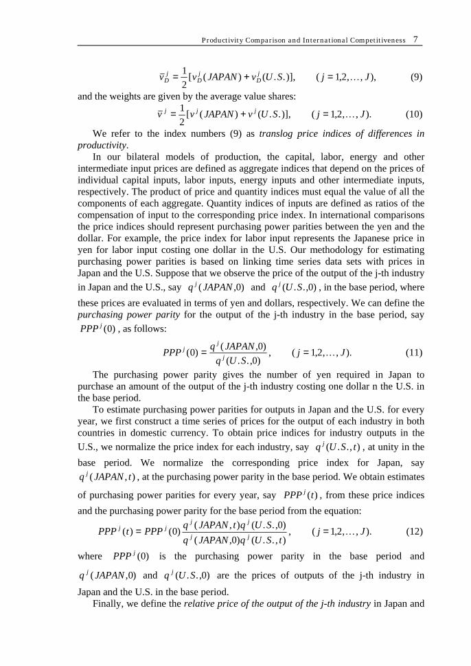
commodities as a factor in the product mix. Our measurement of output in chemicals might not precisely take into account the differences of the product mix in the chemical sector. Differences of the product mix between Japan and the U.S. are not able to measure exactly not only in chemicals, but also other sectors. Even if we include the above qualifications in our results, they still show that productivity levels in the Japanese industries are still behind those in U.S. industries in almost sectors in 1990. We should note that the measurement of the productivity gap does not depend upon the exchange rate. This implies that Japanese industries do not have advantages in competitiveness from the viewpoint of the level of technology during the year 1990. Figure 2 represents the historical trends of the productivity in Japan and the U.S. during the period 1960-95 by industry. Trends after 1993 in both countries are estimated by the simple extension of the data in output and input prices. The level of the productivity index in 1990 is corresponds to the proportional gap between two countries as shown in Figure 1. According to the results in Figure 2, we can classify our 30 industries into several types of technology gaps between two countries.
[Type I]: The U.S. still had an advantage in 1990 in terms of technology. These differences are expected to continue to expand in the future:
Agriculture-forestry-fisheries, coal mining, other mining, foods manuf., apparel, petroleum & coal products, leather products, general machinery, transportation, and communication.
[Type Ⅱ]: The U.S. had a technological advantage in 1990. However, technology gap are almost constant between the two countries:
Woods products, paper & pulp, stone & clay, metal products,
0.65
0.80
0.88
1.22
0.73
0.97
0.90
0.68
1.01
0.74
0.95
1.05
0.84
0.96
0.65
0.97
0.48
0.73
0.86
1.19
1.11
0.88
0.810.79
0.700.67
0.47
1.05
1.32
0.68
0.40
0.50
0.60
0.70
0.80
0.90
1.00
1.10
1.20
1.30
1.Agriculture
2.Coal m
ining
3.Other m
ining
4.Build. &
Const.
5.Foods Prod.
6.Textile
7.Apparel
8.Woods Prod.
9.Furniture
10.Paper & Pulp
11.Publishing
12.Chem
ical Prod.
13.Coal &
Petroleum
14.Leather Prod.
15.Stone & C
lay
16.Primary m
etals
17.Metal Prod.
18.General M
ach.
19.Electric Mach.
20.Motor V
ehicle
21.Other Trans. Equip.
22.Precision Inst.
23.Miscelaneous Prod.
24.Transportation
25.Com
munication
26.Electricity
27.Gas Supply
28.Trade
29.Finance, Insurance
30.Service
Figure 1: Productivity Gap between Japan and U.S. in 1990

Productivity Comparison and International Competitiveness 23
other manuf. electricity, and gas supply. [Type Ⅲ]: The U.S. still had a technological advantage in 1990. But these gaps have been constantly closing since 1960. They are, therefore, expected to close even more in the near future:
Electric machinery and precision instruments. [Type Ⅳ]: Japan had a technological advantage in 1990. These gaps are expected to continue to expand in the future:
Construction, furniture, chemical products, motor vehicle, other transportation equipment, trade, finance, insurance & real estate. [Type V] : Technology levels in both countries are at the almost same level: Primary metals, textiles, and printing. As mentioned previously, we should carefully evaluate the productivity levels in construction, trade and finance. Then, industries in Type Ⅳ only are chemical and motor vehicles. If we take into account the relative trends of productivity in future, only nine industries (including chemical products, motor vehicle, electric machinery, precision instruments, primary metals, textiles, furniture, printing and other transportation equipment) will have an advantages from a technological point of view. Next, we turn to evaluate the international competitiveness of the output price ,by industry. Even in the case in which the level of productivity in industry does not have an advantage in technological terms, there is the possibility of having some international competitiveness at the level of output price, because of the relatively less expensive prices of inputs. As mentioned before, the prices of labor input in Japan are still less expensive in comparison with those in the U.S. Exchange rates might have an influences on the relative level of output prices. Figure 3 represents trends of output prices by industry during the period 1960-95. In Figure 3, the series designated by `JP' shows trend of the output price not adjusted by the changes of exchange rate, while the series designated by‘JP(e-adjusted)’shows trend of output price adjusted by changes of exchange rate.‘US’in Figure 3 shows trend of output price of the corresponding U.S. industry. By the time of appreciation of yen after 1990, almost all industries in Japan lost their competitiveness in terms of output price. In 1995, the motor vehicle sector is the only industry which still has an advantage in terms of output price, where the exchange rate was 94.07 yen to the dollar. On the other hand, in 1990, when the exchange rate was 144.81 yen per dollar, industries which did not have advantages in the level of productivity (such as primary metals, printing, other transportation equipment, precision, and transportation) had advantages from the viewpoint of the comparative level of their output prices. Concerning the relationship between the relative output prices and the proportional gap at the technological level, we can summarize the features of the international competitiveness by industry in Figure 4-6. In Figure 4-6, the horizontal axis is measured by the proportional gap of the technology level between Japan and the U.S., while the vertical axis is measured by the relative price of output in the Japanese industry, compared with the U.S. price. This implies that in the horizontal axis, the larger the value of the horizontal measures is, the more efficient Japanese technology is, while in the vertical axis, the smaller the value of the vertical measures

24 Journal of Applied Input-Output Analysis, Vol. 5, 1999
(rather than unity), the greater advantage the Japanese output price has from the viewpoint of price competitiveness. Three figures, 4-6 represent the plots for industries in 1985,1990 and 1995. We can observe that Japanese industries lost their international competitiveness in terms of the output price, because of the rapid appreciation of yen after 1985. We have to note that the exchange rate (yen to the dollar) continuously appreciated from 238.57 yen in 1985, to 144.81 yen in 1990 and 94.07 yen in 1995. We can see that the plots in Figures have shifted upward, clearly because of the appreciation of yen. Plots for industry might be negatively correlated. The more efficient the levels of productivity are, the more advantageous the international competitiveness, in terms of the level of output price might be. From these considerations, the plots in the fourth quadrant are desirable from viewpoints of the international competitiveness of industry. It is because the international competitiveness of the industries located in the fourth quadrant would be guaranteed by the higher level of the productivity. We can see, however, that there were no industries located in the fourth quadrant in 1995. This suggests that the appreciated yen value completely canceled out the advantage in the level of productivity concerning the level of output price. Plots in the third quadrant imply that the levels of the output price in these industries have a degree of competitiveness in spite of the disadvantages of the level of productivity, because of the relatively cheaper prices of inputs. In 1985, when the exchange rate was 238.57 yen to the dollar, we could find several industries located in the third quadrant, such as apparel, wood products, communication, transportation, trade and services. However, we could not find any industries in the third quadrant in 1990 and 1995. In 1990, when the exchange rate was 144.81 yen to the dollar, we could still find some industries in the fourth quadrant such as construction, chemicals, motor vehicles, and finance. However, in 1995 when the exchange rate was 94.07 yen to the dollar, we could not find any industries in the fourth quadrant. Plots located in the first quadrant imply that the industries located there lost their price competitiveness in spite of the advantages in terms of the level of technology. This is because the exchange rate might be overvalued, or the prices of input might be overvalued for the industry-specific reasons of the market structure. On the other hand, plots in the second quadrant mean that the industries located there lost their competitiveness in terms of output prices; this being because of the lower level of productivity. It might be interest to note that there are included some industries regulated by institutional factors; such as electricity, gas and petroleum & coal products.

Productivity Comparison and International Competitiveness 25
Figure 2: Historical Trends of the TFP in Japan and the U.S.(1)
0.00
0.20
0.40
0.60
0.80
1.00
1.20
1948
1951
1954
1957
1960
1963
1966
1969
1972
1975
1978
1981
1984
1987
1990
1993
1996
US
JP
1.Agriculture
0.00
0.20
0.40
0.60
0.80
1.00
1.20
1.40
1948
1951
1954
1957
1960
1963
1966
1969
1972
1975
1978
1981
1984
1987
1990
1993
1996
US
JP
2.Coal Mining
0.000.200.400.600.801.001.201.401.60
1948
1951
1954
1957
1960
1963
1966
1969
1972
1975
1978
1981
1984
1987
1990
1993
1996
US
JP
3.Other Mining
0.000.20
0.400.600.801.00
1.201.40
1948
1951
1954
1957
1960
1963
1966
1969
1972
1975
1978
1981
1984
1987
1990
1993
1996
US
JP
4.Building & Construction
0.00
0.20
0.40
0.60
0.80
1.00
1.20
1948
1951
1954
1957
1960
1963
1966
1969
1972
1975
1978
1981
1984
1987
1990
1993
1996
US
JP
5.Food & Kindred Products
0.00
0.20
0.40
0.60
0.80
1.00
1.20
1948
1951
1954
1957
1960
1963
1966
1969
1972
1975
1978
1981
1984
1987
1990
1993
1996
US
JP
6.Textile
0.00
0.20
0.40
0.60
0.80
1.00
1.20
1948
1951
1954
1957
1960
1963
1966
1969
1972
1975
1978
1981
1984
1987
1990
1993
1996
US
JP
7.Apparel
0.00
0.20
0.40
0.60
0.80
1.00
1.20
1948
1951
1954
1957
1960
1963
1966
1969
1972
1975
1978
1981
1984
1987
1990
1993
1996
US
JP
8.Wood Products
0.00
0.20
0.40
0.60
0.80
1.00
1.20
1948
1951
1954
1957
1960
1963
1966
1969
1972
1975
1978
1981
1984
1987
1990
1993
1996
US
JP
9.Furniture
0.00
0.20
0.40
0.60
0.80
1.00
1.20
1948
1951
1954
1957
1960
1963
1966
1969
1972
1975
1978
1981
1984
1987
1990
1993
1996
US
JP
10.Paper & Pulp Products
26 Journal of Applied Input-Output Analysis, Vol. 5, 1999
Figure 2: Historical Trends of the TFP in Japan and the U.S.(2)
0.000.200.400.600.80
1.001.201.401.60
1948
1951
1954
1957
1960
1963
1966
1969
1972
1975
1978
1981
1984
1987
1990
1993
1996
US
JP
11.Publishing
0.00
0.20
0.40
0.60
0.80
1.00
1.20
1948
1951
1954
1957
1960
1963
1966
1969
1972
1975
1978
1981
1984
1987
1990
1993
1996
US
JP
12.Chemical Products
0.00
0.20
0.40
0.60
0.80
1.00
1.20
1.40
1948
1951
1954
1957
1960
1963
1966
1969
1972
1975
1978
1981
1984
1987
1990
1993
1996
US
JP
13.Petroleum & Coal Products
0.00
0.20
0.40
0.60
0.80
1.00
1.20
1948
1951
1954
1957
1960
1963
1966
1969
1972
1975
1978
1981
1984
1987
1990
1993
1996
US
JP
14.Leather Products
0.00
0.20
0.40
0.60
0.80
1.00
1.20
1948
1951
1954
1957
1960
1963
1966
1969
1972
1975
1978
1981
1984
1987
1990
1993
1996
US
JP
15.Stone & Clay
0.00
0.20
0.40
0.60
0.80
1.00
1.20
1948
1951
1954
1957
1960
1963
1966
1969
1972
1975
1978
1981
1984
1987
1990
1993
1996
US
JP
16.Primary Metal
0.00
0.20
0.40
0.60
0.80
1.00
1.20
1948
1951
1954
1957
1960
1963
1966
1969
1972
1975
1978
1981
1984
1987
1990
1993
1996
US
JP
17.Metal Products
0.00
0.20
0.40
0.60
0.80
1.00
1.20
1948
1951
1954
1957
1960
1963
1966
1969
1972
1975
1978
1981
1984
1987
1990
1993
1996
US
JP
18.General machinery
0.00
0.20
0.40
0.60
0.80
1.00
1.20
1948
1951
1954
1957
1960
1963
1966
1969
1972
1975
1978
1981
1984
1987
1990
1993
1996
US
JP
19.Electric Machinery
0.00
0.20
0.40
0.60
0.80
1.00
1.20
1.40
1948
1951
1954
1957
1960
1963
1966
1969
1972
1975
1978
1981
1984
1987
1990
1993
1996
US
JP
20.Motor Vehicle

Productivity Comparison and International Competitiveness 27
Figure 2: Historical Trends of the TFP in Japan and the U.S.(3)
0.00
0.20
0.40
0.60
0.80
1.00
1.20
1948
1951
1954
1957
1960
1963
1966
1969
1972
1975
1978
1981
1984
1987
1990
1993
1996
US
JP
21.Other Transportation Equipment
0.00
0.20
0.40
0.60
0.80
1.00
1.20
1948
1951
1954
1957
1960
1963
1966
1969
1972
1975
1978
1981
1984
1987
1990
1993
1996
US
JP
22.Precision Instruments
0.00
0.20
0.40
0.60
0.80
1.00
1.20
1948
1951
1954
1957
1960
1963
1966
1969
1972
1975
1978
1981
1984
1987
1990
1993
1996
US
JP
23.Miscelaneous Products
0.00
0.20
0.40
0.60
0.80
1.00
1.20
1948
1951
1954
1957
1960
1963
1966
1969
1972
1975
1978
1981
1984
1987
1990
1993
1996
US
JP
24.Transportation
0.00
0.20
0.40
0.60
0.80
1.00
1.20
1948
1951
1954
1957
1960
1963
1966
1969
1972
1975
1978
1981
1984
1987
1990
1993
1996
US
JP
25.Communication
0.00
0.20
0.40
0.60
0.80
1.00
1.20
1.40
1948
1951
1954
1957
1960
1963
1966
1969
1972
1975
1978
1981
1984
1987
1990
1993
1996
US
JP
26.Electricity
0.00
0.20
0.40
0.60
0.80
1.00
1.20
1.40
1948
1951
1954
1957
1960
1963
1966
1969
1972
1975
1978
1981
1984
1987
1990
1993
1996
US
JP
27.Gas Utilities
0.00
0.20
0.40
0.60
0.80
1.00
1.2019
48
1951
1954
1957
1960
1963
1966
1969
1972
1975
1978
1981
1984
1987
1990
1993
1996
US
JP
28.Trade
0.000.200.400.600.801.001.201.401.60
1948
1951
1954
1957
1960
1963
1966
1969
1972
1975
1978
1981
1984
1987
1990
1993
1996
US
JP
29.Finance,Insurance & Real Estate
0.00
0.20
0.40
0.60
0.80
1.00
1.20
1.40
1948
1951
1954
1957
1960
1963
1966
1969
1972
1975
1978
1981
1984
1987
1990
1993
1996
US
JP
30.Other Services

28 Journal of Applied Input-Output Analysis, Vol. 5, 1999
Figure 3: Historical Trends of Output Prices in Japan and the U.S.(1)
0.00
0.40
0.80
1.20
1.60
2.00
2.40
1948
1951
1954
1957
1960
1963
1966
1969
1972
1975
1978
1981
1984
1987
1990
1993
1996
JP
JP(e-adjusted)
US
1.Agriculture
0.00
0.40
0.80
1.20
1.60
1948
1951
1954
1957
1960
1963
1966
1969
1972
1975
1978
1981
1984
1987
1990
1993
1996
JP
JP(e-adjusted)
US
2.Coal Mining
0.00
0.50
1.00
1.50
2.00
2.50
3.00
1948
1951
1954
1957
1960
1963
1966
1969
1972
1975
1978
1981
1984
1987
1990
1993
1996
JP
JP(e-adjusted)
US
3.Other Mining
0.00
0.50
1.00
1.50
2.00
1948
1951
1954
1957
1960
1963
1966
1969
1972
1975
1978
1981
1984
1987
1990
1993
1996
JP
JP(e-adjusted)
US
4.Building & Construction
0.00
0.50
1.00
1.50
2.00
2.50
3.00
3.50
1948
1951
1954
1957
1960
1963
1966
1969
1972
1975
1978
1981
1984
1987
1990
1993
1996
JP
JP(e-adjusted)
US
5.Food & Kindred Products
0.00
0.40
0.80
1.20
1.60
1948
1951
1954
1957
1960
1963
1966
1969
1972
1975
1978
1981
1984
1987
1990
1993
1996
JP
JP(e-adjusted)
US
6.Textile
0.00
0.50
1.00
1.50
2.00
1948
1951
1954
1957
1960
1963
1966
1969
1972
1975
1978
1981
1984
1987
1990
1993
1996
JP
JP(e-adjusted)
US
7.Apparel
0.00
0.50
1.00
1.50
2.00
2.50
1948
1951
1954
1957
1960
1963
1966
1969
1972
1975
1978
1981
1984
1987
1990
1993
1996
JP
JP(e-adjusted)
US
8.Wood Products
0.00
0.50
1.00
1.50
2.00
1948
1951
1954
1957
1960
1963
1966
1969
1972
1975
1978
1981
1984
1987
1990
1993
1996
JP
JP(e-adjusted)
US
9.Furniture
0.00
0.50
1.00
1.50
2.00
2.50
1948
1951
1954
1957
1960
1963
1966
1969
1972
1975
1978
1981
1984
1987
1990
1993
1996
JP
JP(e-adjusted)
US
10.Paper & Pulp Products

Productivity Comparison and International Competitiveness 29
Figure 3: Historical Trends of Output Prices in Japan and the U.S.(2)
0.00
0.40
0.80
1.20
1.60
2.00
1948
1951
1954
1957
1960
1963
1966
1969
1972
1975
1978
1981
1984
1987
1990
1993
1996
JP
JP(e-adjusted)
US
11.Publishing
0.00
0.40
0.80
1.20
1.60
1948
1951
1954
1957
1960
1963
1966
1969
1972
1975
1978
1981
1984
1987
1990
1993
1996
JP
JP(e-adjusted)
US
12.Chemical Products
0.000.501.001.502.002.503.003.504.004.50
1948
1951
1954
1957
1960
1963
1966
1969
1972
1975
1978
1981
1984
1987
1990
1993
1996
JP
JP(e-adjusted)
US
13.Petroleum & Coal Products
0.00
0.40
0.80
1.20
1.60
2.00
2.40
1948
1951
1954
1957
1960
1963
1966
1969
1972
1975
1978
1981
1984
1987
1990
1993
1996
JP
JP(e-adjusted)
US
14.Leather Products
0.00
0.40
0.80
1.20
1.60
2.00
1948
1951
1954
1957
1960
1963
1966
1969
1972
1975
1978
1981
1984
1987
1990
1993
1996
JP
JP(e-adjusted)
US
15.Stone & Clay
0.00
0.40
0.80
1.20
1.60
1948
1951
1954
1957
1960
1963
1966
1969
1972
1975
1978
1981
1984
1987
1990
1993
1996
JP
JP(e-adjusted)
US
16.Primary Metal
0.00
0.50
1.00
1.50
2.00
2.50
3.00
3.50
1948
1951
1954
1957
1960
1963
1966
1969
1972
1975
1978
1981
1984
1987
1990
1993
1996
JP
JP(e-adjusted)
US
17.Metal Products
0.00
0.50
1.00
1.50
2.00
2.50
3.00
1948
1951
1954
1957
1960
1963
1966
1969
1972
1975
1978
1981
1984
1987
1990
1993
1996
JP
JP(e-adjusted)
US
18.General Machinery
0.00
0.40
0.80
1.20
1.60
2.00
1948
1951
1954
1957
1960
1963
1966
1969
1972
1975
1978
1981
1984
1987
1990
1993
1996
JP
JP(e-adjusted)
US
19.Electric Machinery
0.00
0.40
0.80
1.20
1.60
1948
1951
1954
1957
1960
1963
1966
1969
1972
1975
1978
1981
1984
1987
1990
1993
1996
JP
JP(e-adjusted)
US
20.Motor Vehicle

30 Journal of Applied Input-Output Analysis, Vol. 5, 1999
Figure 3: Historical Trends of Output Prices in Japan and the U.S.(3)
0.00
0.40
0.80
1.20
1.60
2.00
1948
1951
1954
1957
1960
1963
1966
1969
1972
1975
1978
1981
1984
1987
1990
1993
1996
JP
JP(e-adjusted)
US
21.Other Transportation Equipment
0.00
0.40
0.80
1.20
1.60
2.00
1948
1951
1954
1957
1960
1963
1966
1969
1972
1975
1978
1981
1984
1987
1990
1993
1996
JP
JP(e-adjusted)
US
22.Precision Instruments
0.00
0.40
0.80
1.20
1.60
2.00
2.40
1948
1951
1954
1957
1960
1963
1966
1969
1972
1975
1978
1981
1984
1987
1990
1993
1996
JP
JP(e-adjusted)
US
23.Miscelaneous Products
0.00
0.40
0.80
1.20
1.60
2.00
1948
1951
1954
1957
1960
1963
1966
1969
1972
1975
1978
1981
1984
1987
1990
1993
1996
JP
JP(e-adjusted)
US
24.Transportation
0.00
0.50
1.00
1.50
2.00
2.50
1948
1951
1954
1957
1960
1963
1966
1969
1972
1975
1978
1981
1984
1987
1990
1993
1996
JP
JP(e-adjusted)
US
25.Communication
0.00
0.50
1.00
1.50
2.00
2.50
3.00
1948
1951
1954
1957
1960
1963
1966
1969
1972
1975
1978
1981
1984
1987
1990
1993
1996
JP
JP(e-adjusted)
US
26.Electricity
0.000.501.001.502.002.50
3.003.504.00
1948
1951
1954
1957
1960
1963
1966
1969
1972
1975
1978
1981
1984
1987
1990
1993
1996
JP
JP(e-adjusted)
US
27.Gas Utilities
0.00
0.40
0.80
1.20
1.60
1948
1951
1954
1957
1960
1963
1966
1969
1972
1975
1978
1981
1984
1987
1990
1993
1996
JP
JP(e-adjusted)
US
28.Trade
0.00
0.40
0.80
1.20
1.60
1948
1951
1954
1957
1960
1963
1966
1969
1972
1975
1978
1981
1984
1987
1990
1993
1996
JP
JP(e-adjusted)
US
29.Finance,Insurance & Real Estate
0.00
0.40
0.80
1.20
1.60
2.00
1948
1951
1954
1957
1960
1963
1966
1969
1972
1975
1978
1981
1984
1987
1990
1993
1996
JP
JP(e-adjusted)
US
30.Other Services

Productivity Comparison and International Competitiveness 31
Figure 4: International Competitiveness in 1985
Figure 5: International Competitiveness in 1990
0.00
0.50
1.00
1.50
2.00
2.50
0.30 0.60 0.90 1.20
Gas
Metal Products
Petroleumn & Coal Products
Finance,Insurance& Real EstateMotor
Vehicle
Coal Mining
Electric Machinery General
Machinery
Transportation
Communication
Electricity
Foods
Agriculture
Building& Construction
Other Service
Chemicals
Pd
highlow
Comparison of Relative Total Factor Productivity and Output Pricebetween Japan and US in 1985(Exchange Rate =¥238.57/$)
TFP(Japan/U.S.)
Pd (Japan/U.S.)
TFP highlow
Paper& Pulp Products
WoodProducts
TradeApparel
0.50
1.00
1.50
2.00
2.50
0.40 0.70 1.00 1.30
Gas
Metal Products
Petroleumn & Coal Products
Finance,Insurance& Real Estate
Motor Vehicle
Other Mining
Coal Mining
Electric Machinery
General Machinery
Transportation
Communication
ElectricityFoods
Agriculture
Building& Construction
Other Service
Chemicals
LeatherProducts
PrecisionInstruments
Pd
highlow
Comparison of Relative Total Factor Productivity and Output Pricebetween Japan and US in 1990(Exchange Rate =¥144.81/$)
TFP(Japan/U.S.)
Pd (Japan/U.S.)
TFP highlow
Textile
Furniture

32 Journal of Applied Input-Output Analysis, Vol. 5, 1999
Figure 6: International Competitiveness in 1995
5. Conclusions We can summarize the proportional technology gap by industry as an index for the aggregated level of total factor productivity in both Japan and the U.S. Figure 7 represents series of aggregated total factor productivity indices in Japan and the U.S. during the period 1960-95. In Figure 7, indices are normalized at the level of productivity in the U.S. at the year 1990. We can compare the level of the productivity at the aggregated level in Japan and the U.S. As mentioned before, the levels of total factor productivity in Figure 7 are neutral in terms of the changes of exchange rate. In the 1960s, especially during the first half, the growth rate of productivity in Japan was significantly higher than that in the U.S. During this period, the proportional technology gap rapidly diminished. The oil crisis had an enormous impact on the Japanese economy and the gap then expanded again. Although we could observe the restoration of the growth rate of productivity in Japan after 1980, the growth rate was not higher than that in the 1960s. During the period 1960-95, the annual average growth rate of total factor productivity in Japan was 1.052 percent, while that in the U.S. was 0.597 percent. This suggests that the level of technology in Japan has been gradually catching up with the U.S. level during the period 1960-90, but the proportional gap was still dominant in 1995, in terms of the macro aggregate view. Instead of the index of total factor productivity, we can estimate the partial indices of factor inputs, labor and capital. Labor productivity at the aggregated level was defined by a ratio of the aggregated value-added; deflated by the relative price
0.50
1.00
1.50
2.00
2.50
3.00
3.50
4.00
0.40 0.70 1.00 1.30 1.60
Gas
Metal Products
Petroleumn & Coal Products
Finance,Insurance& Real EstateMotor Vehicle
Other Mining
Electric Machinery
General Machinery
Transportation
Communication
Electricity Foods
Agriculture
Building& Construction
Other Service
Chemicals
LeatherProducts
PrecisionInstruments
Pd
highlow
Comparison of Relative Total Factor Productivity and Output Pricebetween Japan and US in 1995(Exchange Rate =¥94.07/$)
TFP(Japan/U.S.)
Pd (Japan/U.S.)
TFP highlow
Textile
Furniture
Trade

Productivity Comparison and International Competitiveness 33
index adjusted by the PPP index to the aggregated labor compensation; deflated by the relative price index of labor input; adjusted by the PPP index. Capital productivity at the aggregated level was also defined in the same way as labor productivity. It is a ratio of the aggregated value-added; deflated by the relative price index; adjusted by the PPP index to the aggregated capital compensation; deflated by the relative price index of capital input adjusted by the PPP index. We should note that partial productivity of both labor and capital as shown in Figure 8 and 9 are neutral in terms of the changes of the exchange rate. The growth rate of labor productivity in Japan was relatively high in comparison with that in the U.S. The level of labor productivity in Japan was still lower than that in the U.S. On the other hand, capital productivity in Japan has been diminishing rapidly since 1960, because of the accelerated accumulation of capital. The level of capital productivity was stabilizing in the 1980s and the difference between two countries almost decreased during the second half of the decade. We can characterize the development of labor productivity as the process of the substitution between labor and capital, where the labor productivity increased rapidly at the cost of declining capital productivity. Finally, we can estimate the theoretical value of the exchange rate between Japan and the U.S., where prices, adjusted by the exchange rate were equalized in both countries. Figure 10 represent the series of theoretical value of the exchange rate with the observed value of that, where we assume the prices of gross output at the aggregated level would be equalized in both countries. During the period 1960-71, when the observed exchange rate was fixed at 360.0 yen to the dollar, the observed value of the exchange rate was significantly higher than the theoretical value. This implies that the observed value could be undervalued. After the shift to the floating system in the exchange market in 1971, the difference between the observed and the theoretical values was gradually reduced. During the period 1977-81, the observed value was lower than the theoretical value, which means the observed exchange rate could be overvalued. Although the observed exchange rate shifted again during the period 1982-86, it has again been lower than the theoretical value since 1986. It means that the observed value was overvalued, in comparison with the theoretical value. According to our results, the theoretical value of the exchange rate, where the relative price of gross output at the aggregated level was completely balanced between Japan and the U.S., would be around 160.0 yen in 1995. We should note, however, that this estimated value of the exchange rate is completely dependent upon the selected index of prices to be compared. We can select the relative price index of factor costs in order to estimate the theoretical value of exchange rate. If we try to estimate the value of the exchange rate, where the factor prices are equalized between both countries, we could obtain 125.0 yen to the dollar as the theoretical value of exchange rate in 1995. The difference of both theoretical values between 160.0 and 125.0 yen is almost 30 percent, which is corresponds consistently with the difference in productivity in 1995. We will summarize our results of international comparisons between Japan and the U.S. As mentioned previously, the period 1960-70 was characterized by substantial economic growth in the U.S. and very rapid economic growth in Japan. Capital input was by far the most important source of growth in both countries. The period 1973-1979 was dominated by the energy crisis, which began with drastic increases in petroleum prices in 1973. Growth slowed significantly in the U.S. and

34 Journal of Applied Input-Output Analysis, Vol. 5, 1999
declined dramatically in Japan during this period. The growth of capital input remained the most important source of economic growth in both countries, but contribution of the productivity growth at the sectoral level essentially disappeared. During the period 1960-1973, productivity growth in Japan exceeded that in the U.S. in almost all industries. After the energy crisis in 1973, there were very few significant differences between growth rates of productivity in Japanese and U.S. industries. An important focus of our work has been the assessment of long term trends in productivity growth. In particular, we have tried to establish whether or not the slowdown in productivity growth in Japan and the U.S., after the energy crisis has become permanent. Although our observation of the productivity trend since 1980s' in both countries represented a slight recovery from the shock in the oil crisis, the growth rates of the productivity still were moderate. The second issue we have considered is the trend of industry-level productivity differences between the two countries. Jorgenson, Kuroda, and Nishimizu (1987) and Jorgenson and Kuroda (1990) showed that almost all sectors of Japanese industry had a lower level of productivity than their U.S. counterparts in 1960. By the period 1990 there were seven industries in which the productivity gaps between the two countries had closed. These industries were primarily concentrated in producer's goods manufacturing, and were focused on export-oriented industries. In the remaining 23 industries, productivity gaps between Japan and the U.S. remained in 1990. According to our results, extended until 1995, the proportional technology gaps between both countries have not diminished in almost all industries in 1995 as of yet. After 1973, productivity growth deteriorated substantially in both Japan and the United States. An important issue is whether the productivity slowdown is a permanent features in both economies. To resolve this issue we can consider average productivity growth rates in Japanese and U.S. industries over the period 1960-95: Japan U.S. 1960-65 5.402 2.236 1965-70 6.223 0.793 1970-73 - 0.085 2.084 1973-75 - 2.624 - 2.595 1975-80 0.014 - 0.005 1980-85 1.070 0.963 1985-90 1.306 0.461 1990-95 0.548 - 0.529 We conclude that productivity growth in Japan and the U.S. has revived slightly since 1980. However, the growth rates for the period 1980-1985 are well below those for the period 1960-1973, especially in Japan.

Productivity Comparison and International Competitiveness 35
Figure 7: Aggregated Level of TFP in Japan and the U.S.
Figure 8: Aggregated Level of Labor Productivity in Japan and the U.S.
0.40
0.50
0.60
0.70
0.80
0.90
1.00
1.10
1948
1950
1952
1954
1956
1958
1960
1962
1964
1966
1968
1970
1972
1974
1976
1978
1980
1982
1984
1986
1988
1990
1992
1994
1996
US
Japan
0.20
0.30
0.40
0.50
0.60
0.70
0.80
0.90
1.00
1.10
1948
1950
1952
1954
1956
1958
1960
1962
1964
1966
1968
1970
1972
1974
1976
1978
1980
1982
1984
1986
1988
1990
1992
1994
1996
US
Japan
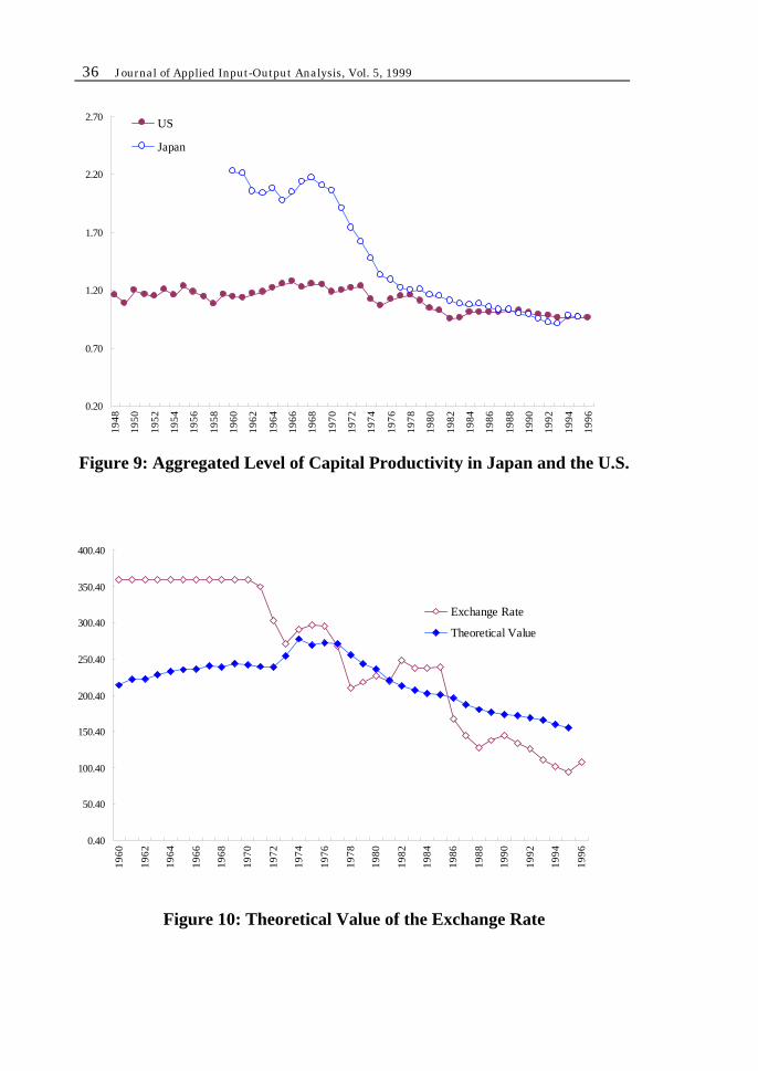
36 Journal of Applied Input-Output Analysis, Vol. 5, 1999
Figure 9: Aggregated Level of Capital Productivity in Japan and the U.S.
Figure 10: Theoretical Value of the Exchange Rate
0.20
0.70
1.20
1.70
2.20
2.7019
48
1950
1952
1954
1956
1958
1960
1962
1964
1966
1968
1970
1972
1974
1976
1978
1980
1982
1984
1986
1988
1990
1992
1994
1996
US
Japan
0.40
50.40
100.40
150.40
200.40
250.40
300.40
350.40
400.40
1960
1962
1964
1966
1968
1970
1972
1974
1976
1978
1980
1982
1984
1986
1988
1990
1992
1994
1996
Exchange Rate
Theoretical Value

Productivity Comparison and International Competitiveness 37
References [1] Caves,D.W., L.R.Christensen and W.E.Diewert (1982), “Multilateral Comparisons of
Output, Input, and Productivity Using Surperlative Index Numbers”, Economic Journal, Vol.92,No.365, March, pp.73-86.
[2] Chistensen, L.R., D.Commings, and D.W. Jorgenson (1981), “Relative Productivity Levels, 1947-1979”, Eupopean Ecomonic Reviews, Vol.16,No.1,May, pp.61-94.
[3] Hall, R. E.(1968), “Technical Change and Capital from the Point of View of the Dual”, The Review of Economic Studies, Vol. 35, pp.35-46.
[4] Hall, R. E. and D.W. Jorgenson( 1967), “Tax Policy and Investment Behavior”, American Economic Review, Vol..57, pp.391-414.
[5] Jorgenson, D.W.(1963), “Capital Theory and Investment Behavior”, American Economic Review, Vol.53, pp.247-274.
[6] Jorgenson, D.W. and Z. Griliches (1967), “The Explanation of Productivity Change”, The Review of Economic Studies, Vol.34, pp.249-283.
[7] Jorgenson, D. W. and M. Nishimizu (1978), “U.S. and Japanses Economic Growth, 1952-1974: An International Comparison”, Economic Journal,Vol.88, No.352, pp.707-726.
[8] Jorgenson, D.W., M. Kuroda and M. Nishimizu (1987), “Japan-U.S. Industry-Level Productivity Comparisons, 1960-1979”, Journal of the Japanese and International Economics, Vol.1, No.1, March, pp.1-31.
[9] Jorgenson, D.W., M. Kuroda, and M. Nishimizu (1988), “Productivity and Economic Growth in Japan and the United States”, American Economic Review, Vol.78, No.2, pp.217-222.
[10] Jorgenson, D.W., and M. Kuroda (1990), “Productivity and International Competitiveness in Japan and the United States, 1960-1985”, in C.R. Hulten, eds., Productivity Growth in Japan and the United States, Studies in Income and Wealth, vol.53, University of Chicago Press, pp.29-55.
[11] Kuroda, M (1988), “A Method of Estimation for Updating Transaction Matrix in the Input-Output Relationship”, in Uno, K, and S. Shishido, eds., Statistical Data Bank Systems, Socio-Economic Database and Model Building in Japan, North-Holland : Amsterdam, Chapter 2, pp.19-118.
[12] Kuroda, M., K. Shimpo, K. Nomura and N. Kobayashi (1994),KEO Data Base: Output, Labor and Capital, Sangyou Kenkyujo Monograph Series (in Japanese).
[13] Solow, R. M (1955), “The Production Function and the Theory of Capital”, The Review of Economic Studies, Vol.23, pp.101-108.