Product Mix and Firm Productivity Responses to TradeCompetition

Thierry Mayer

Sciences-PoCEPII and CEPR

Marc J. Melitz

Harvard UniversityNBER and CEPR

Gianmarco I.P. Ottaviano

London School of EconomicsU Bologna, CEP and CEPR

December 2014

PRELIMINARY AND INCOMPLETE DRAFT

1 Introduction

In this paper, we document how demand shocks in export markets lead French multi-product

exporters to re-allocate the product mix sold in those destinations. We develop a theoretical model

of multi-product firms that highlight the specific demand and cost conditions needed to generate all

those empirical predictions. We then show how the increased competition from the demand shocks

in export markets —and the associated product mix responses — lead to substantial productivity

improvements for multi-product exporters.

Recent studies using detailed micro-level datasets on firms, plants, and the products they pro-

duce have documented vast differences in all measurable performance metrics across those different

units. Those studies have also documented that these performance differences are systematically

related to participation in international markets (see, e.g., Mayer and Ottaviano (2008) for Europe,

and Bernard, Jensen, Redding and Schott (2012) for the U.S.): Exporting firms and plants are

bigger, more productive, more profitable, and less likely to exit than non-exporters. And better

performing firms and plants export a larger number of products to a larger number of destinations.

Exporters are larger in terms of employment, output, revenue and profit. Similar patterns also

emerge across the set of products sold by multi-product firms. There is a stable performance rank-

ing for firms based on the products’performance in any given market, or in worldwide sales. Thus,

better performing products in one market are most likely to be the better performing products in

any other market (including the global export market). This also applies to the products’selection

into a destination, so better performing products are also sold in a larger set of destinations.

Given this heterogeneity, trade shocks induce many different reallocations across firms and

products. Some of these reallocations are driven by ‘selection effects’that determine which products

are sold where (across domestic and export markets), along with firm entry/exit decisions (into/out

of any given export market, or overall entry/exit of the firm). Other reallocations are driven by

‘competition effects’whereby — conditional on selection (a given set of products sold in a given

market) —trade affects the relative market shares of those products. Both types of reallocations

generate (endogenous) productivity changes that are independent of ‘technology’(the production

function at the product-level). This creates an additional channel for the aggregate gains from

trade.

Unfortunately, measuring the direct impact of trade on those reallocations across firms is a

very hard task. On one hand, shocks that affect trade are also likely to affect the distribution

1

of market shares across firms. On the other hand, changes in market shares across firms likely

reflect many technological factors (not related to reallocations). Looking at reallocations across

products within firms obviates some of these problems. Recent theoretical models of multi-product

firms highlight how trade induces a similar pattern of reallocations within firms as it does across

firms. And measuring reallocations within multi-product firms has several advantages: Trade

shocks that are exogenous to individual firms can be identified much more easily than at a higher

level of aggregation; Controls for any technology changes at the firm-level are also possible; and

reallocations can be measured for the same set of narrowly defined products sold by same firm

across destinations or over time. Moreover, multi-product firms dominate world production and

trade flows. Hence, reallocations within multi-product firms have the potential to generate large

changes in aggregate productivity. Empirically, we find very strong evidence for the effects of trade

shocks on those reallocations, and ultimately on the productivity of multi-product firms. The

overall impact on aggregate French manufacturing productivity is substantial.

2 Previous Evidence on Trade-Induced Reallocations

In a previous paper, Mayer, Melitz and Ottaviano (2014), we investigated, both theoretically and

empirically, the mechanics of these reallocations within multi-product firms. We used a compre-

hensive firm-level data on annual shipments by all French exporters to all countries in the world

(not including the French domestic market) for a set of more than 10,000 goods. Firm-level exports

are collected by French customs and include export sales for each 8-digit (combined nomenclature

or NC8) product by destination country. Our focus then was on the cross-section of firm-product

exports across destinations (for a single year, 2003). We presented evidence that French multi-

product firms indeed exhibit a stable ranking of products in terms of their shares of export sales

across export destinations with ‘core’products being sold in a larger number of destinations (and

commanding larger market shares across destinations). We used the term ‘skewness’ to refer to

the dispersion of these export market shares in any destination and showed that this skewness

consistently varied with destination characteristics such as GDP and geography: French firms sold

relatively more of their best performing products in bigger, more centrally-located destinations

(where competition from other exporters and domestic producers is tougher).

Other research has also documented similar patterns of product reallocations (within multi-

product firms) over time following trade liberalization. For the case of CUSFTA/NAFYA, Baldwin

and Gu (2009), Bernard, Redding and Schott (2011), and Iacovone and Javorcik (2008) all report

2

that Canadian, U.S., and Mexican multi-product firms reduced the number of products they pro-

duce during these trade-liberalization episodes. Baldwin and Gu (2009) and Bernard, Redding and

Schott (2011) further report that CUSFTA induced a significant increase in the skewness of pro-

duction across products. Iacovone and Javorcik (2008) separately measure the skewness of Mexican

firms’export sales to the US. They report an increase in this skewness following NAFTA: They

show that Mexican firms expanded their exports of their better performing products (higher mar-

ket shares) significantly more than those for their worse performing exported products during the

period of trade expansion from 1994− 2003.

As prices are rarely observed, there is little direct evidence on how markups, prices and costs

are related across products supplied with different productivity, and how they respond to trade

liberalization.1 A notable exception is the recent paper by DeLoecker, Goldberg, Pavcnik and

Khandelwal (2012) who exploit unique information on the prices and quantities of Indian firms’

products over India’s trade liberalization period from 1989−2003. They also document that better

performing firms (higher sales and productivity) produce more products. They then focus on

markups. Across firms, they document that those better performing firms set higher markups.

They also document a similar patter across the products produced by a given multi-product firm,

which sets relatively higher markups on their better performing products (lower marginal cost and

higher market shares). In addition, they show strong evidence for endogenous markup adjustments

via imperfect pass-through from products’marginal costs to their prices: Only a portion of marginal

cost decreases are passed on to consumers in the form of lower prices, while the remaining portion

goes to higher markups. This is consistent with recent firm-level evidence on exchange rate pass-

through. Berman, Martin and Mayer (2012) analyze the heterogeneous reaction of exporters to

real exchange rate changes using a rich French firm-level data set with destination specific export

values and volumes on the period 1995−2005. They find that on average firms react to depreciation

by increasing their markup. They also find that high-performance firms increases their markup

significantly more —implying that the pass-through rate is significantly lower for better performing

firms.

3 Reallocations Over Time

We now document how changes within a destination market over time induce a similar pattern

of reallocations as the ones we previously described. More specifically, we show that demand

1Prices are typically backed-out as unit values based on reported quantity information, which is extremely noisy.

3

shocks in any given destination market induce firms to skew their product level export sales to that

destination towards their best performing products. In terms of first moments, we show that these

demand shocks also lead to strong positive responses in both the intensive and extensive margins

of export sales to that destination.

3.1 Data

We use the same data as Mayer, Melitz and Ottaviano (2014), the only difference being multiple

years 1995− 2005 instead of a single year 2003. Besides what we already discussed, the reporting

criteria for all firms operating in the French metropolitan territory are as follows. For within EU

exports, the firm’s annual trade value exceeds 100,000 Euros;2 and for exports outside the EU, the

exported value to a destination exceeds 1,000 Euros or a weight of a ton. Despite these limitations,

the database is nearly comprehensive. For instance, in 2003, 100,033 firms report exports across

229 destination countries (or territories) for 10,072 products. This represents data on over 2 million

shipments.

We restrict our analysis to export data in manufacturing industries, mostly eliminating firms

in the service and wholesale/distribution sector to ensure that firms take part in the production of

the goods they export.3 This leaves us with data on over a million shipments by firms in the whole

range of manufacturing sectors.4

3.2 Measuring Trade Shocks

Consider a firm i who exports a number of products s in industry I to destination d in year

t. We measure industries (I) at the 3-digit ISIC level (35 different classifications across French

manufacturing). We consider several measures of demand shocks that affect this export flow. At

the most aggregate level we use the variation in GDP in d, logGDPd,t. At the industry level

I, we use total imports into d excluding French exports, logM Id,t. We can also use our detailed

product-level shipment data to construct a firm i-specific demand shock:

shockIi,d,t ≡ logM sd,t for all products s ∈ I exported by firm i to d in year t0, (1)

2 If that threshold is not met, firms can choose to report under a simplified scheme without supplying export des-tinations. However, in practice, many firms under that threshold report the detailed export destination information.

3Some large distributors such as Carrefour account for a disproportionate number of annual shipments.4 In a robustness check, we also drop observations for firms that the French national statistical institute reports as

having an affi liate abroad. This avoids the issue that multinational firms may substitute exports of some of their bestperforming products with affi liate production in the destination country, thus reducing noise in the product exportskewness. Results are quantitatively very similar in all regressions.

4

where M sd,t represents total imports into d (again, excluding French exports) for product s. For

world trade, the finest level of product level of aggregation is the HS-6 level (from UN-COMTRADE

and CEPII-BACI), which is slightly more aggregated than our NC8 classification for French exports

(roughly 5,300 HS products per year versus 10,000 NC8 products per year). The construction of

this last trade shock is very similar to the one for the industry level imports logM Id,t, except that

we only use imports into d for the precise product categories that firm i exports to d.5 In order

to ensure that this demand shock is exogenous to the firm, we use the set of products exported

by the firm in its first export year in our sample (1995, or later if the firm starts exporting later

on in our sample), and then exclude this year from our subsequent analysis. Note that we use

an un-weighted average so that the shocks for all exported products s (within an industry I) are

represented proportionately.

For all of these demand shocks Xt = GDPd,t,MId,t,M

sd,t, we compute the first difference as the

Davis-Haltiwanger growth rate: ∆Xt ≡ (Xt −Xt−1) / (.5Xt + .5Xt−1). This measure of the first

difference preserves observations when the shock switches from 0 to a positive number, and has a

maximum growth rate of −2 or 2. This is mostly relevant for our measure of the firm-specific trade

shock, where the product-level imports into d, M sd,t can often switch between 0 and positive values.

Whenever Xt−1, Xt > 0, ∆Xt is monotonic in ∆ logXt and approximately linear for typical growth

rates (|∆ logXt| < 2).6 We thus obtain our three measures of trade shocks in first differences:

∆GDPd,t, ∆MId,t,∆M

sd,t. For the firm i-specific shock ∆M s

d,t, we take the un-weighted average of

the growth rates for all products exported by the firm in t− 1.

3.3 The Impact of Demand Shocks on Trade Margins and Skewness

Before focusing on the effects of the demand shocks on the skewness of export sales, we first show

how the demand shocks affect firm export sales at the intensive and extensive margins (the first

moments of the distribution of product export sales). Table 1 reports how our three demand shocks

(in first differences) affect changes in firm exports to destination d in ISIC I (so each observation

represents a firm-destination-ISIC combination). We decompose the firm’s export response to each

shock into an intensive margin (average exports per product) and an extensive margin (number of

exported products). We clearly see how all three demand shocks induce very strong (and highly

5There is a one-to-many matching between the NC8 and HS6 product classifications, so every NC8 product isassigned a unique HS6 classification. We use the same Ms

d,t data for any NC8 product s within the same HS6classification.

6Switching to first difference growth rates measured as ∆ logXt (and dropping products with zero trade in thetrade shock average) does not materially affect any of our results.

5

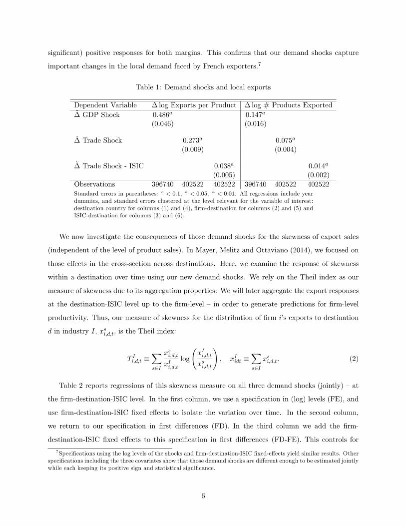
significant) positive responses for both margins. This confirms that our demand shocks capture

important changes in the local demand faced by French exporters.7

Table 1: Demand shocks and local exports

Dependent Variable ∆ log Exports per Product ∆ log # Products Exported∆ GDP Shock 0.486a 0.147a

(0.046) (0.016)

∆ Trade Shock 0.273a 0.075a

(0.009) (0.004)

∆ Trade Shock - ISIC 0.038a 0.014a

(0.005) (0.002)Observations 396740 402522 402522 396740 402522 402522Standard errors in parentheses: c < 0.1, b < 0.05, a < 0.01. All regressions include yeardummies, and standard errors clustered at the level relevant for the variable of interest:destination country for columns (1) and (4), firm-destination for columns (2) and (5) andISIC-destination for columns (3) and (6).

We now investigate the consequences of those demand shocks for the skewness of export sales

(independent of the level of product sales). In Mayer, Melitz and Ottaviano (2014), we focused on

those effects in the cross-section across destinations. Here, we examine the response of skewness

within a destination over time using our new demand shocks. We rely on the Theil index as our

measure of skewness due to its aggregation properties: We will later aggregate the export responses

at the destination-ISIC level up to the firm-level — in order to generate predictions for firm-level

productivity. Thus, our measure of skewness for the distribution of firm i’s exports to destination

d in industry I, xsi,d,t, is the Theil index:

T Ii,d,t ≡∑s∈I

xsi,d,t

xIi,d,tlog

(xIi,d,txsi,d,t

), xIidt ≡

∑s∈I

xsi,d,t. (2)

Table 2 reports regressions of this skewness measure on all three demand shocks (jointly) —at

the firm-destination-ISIC level. In the first column, we use a specification in (log) levels (FE), and

use firm-destination-ISIC fixed effects to isolate the variation over time. In the second column,

we return to our specification in first differences (FD). In the third column we add the firm-

destination-ISIC fixed effects to this specification in first differences (FD-FE). This controls for

7Specifications using the log levels of the shocks and firm-destination-ISIC fixed-effects yield similar results. Otherspecifications including the three covariates show that those demand shocks are different enough to be estimated jointlywhile each keeping its positive sign and statistical significance.

6

any trend growth rate in our demand shocks over time. Across all three specifications, we see

that positive (negative) demand shocks induce a highly significant increase in the skewness of firm

export sales to a destination.8 Next, we construct a measure of the change in skewness restricted

to the subset of products s exported in both periods (for the first difference specifications). This

alternate skewness measure ∆T I,consti,d,t isolates changes that are driven only by the intensive margin

of exports. The two first-difference specifications using this alternate skewness measure are reported

in the last two columns. The effects of our firm-level trade shock is still highly significant (well

beyond the 1% level), whereas the effects based on the ISIC-level trade shock are teetering at the

5% significance level. However, those columns show that the GDP shocks tend to proportionately

change the export sales of ‘incumbent’products. The effect of the GDP shock on skewness thus

comes entirely from the extensive margin (new products exported in response to higher GDP levels

in a destination).9

Table 2: Demand shocks and local skewness

Dependent Variable T Ii,d,t ∆T Ii,d,t ∆T I,consti,d,t

Specification FE FD FD-FE FD FD-FEGDP Shock 0.076a

(0.016)

Trade Shock 0.047a

(0.005)

Trade Shock - ISIC 0.002a

(0.000)

∆ GDP Shock 0.067a 0.068a -0.005 -0.004(0.012) (0.016) (0.008) (0.009)

∆ Trade Shock 0.036a 0.032a 0.012a 0.012a

(0.005) (0.006) (0.003) (0.003)

∆ Trade Shock - ISIC 0.006a 0.004 0.002 0.004b

(0.002) (0.003) (0.001) (0.002)Observations 474506 396740 396740 437626 437626Standard errors in parentheses: c < 0.1, b < 0.05, a < 0.01. All regressions include yeardummies, and standard errors clustered at the level of the destination country.

8The effect of all three shocks are weakened a little bit due to some collinearity. Even in the FD-FE specification,the ISIC-level shock remains significant at the 1% level when it is entered on its own.

9These newly exported products have substantially smaller market shares than the incumbent products andtherefore contribute to an increase in the skewness of export sales.

7

4 Theory

In the previous section we documented the pattern of product reallocations in response to demand

shocks in export markets. We now develop a theoretical model of multi-product firms that highlights

the specific demand conditions needed to generate this pattern. Our theory shows that these

demand conditions imply that the demand shocks lead to increased competition for exporters in

those markets. In addition, we show how this increased competition and the associated product

mix responses lead to higher firm productivity. Finally, we also show that the demand conditions

needed to predict the observed pattern of reallocations to demand shocks are the same that are

needed to predict the relation among firm/product performance measures discussed in Section 2.

In particular, we first present a flexible model with both single- and multi-product firms char-

acterizing the properties of the demand system that are needed to predict the observed relation

between firm/product performance measures. We then show that these properties necessarily im-

ply the documented the pattern of product reallocations in response to demand shocks in export

markets. This is our main point of departure relative to the recent literature focusing on more

flexible demand systems in monopolistic competition models of trade.10

4.1 Closed Economy

To better highlight the role played by the properties of the demand system, we initially start with

a closed economy. We will then move to the open economy to discuss the trade shocks and their

effects.

Multi-Product Production with Additive Separable Utility

Consider an economy populated by Lw identical households, each consisting of η workers. Thus,

each worker supplies 1/η effi ciency units of labor inelastically so that labor supply equals Lw while

the total number of consumers equals Lc = ηLw. Labor is the only productive factor and effi ciency

units of labor per worker are chosen as numeraire so that each consumer earns unit wage (and

household income is η). We think of a demand shock as a change in η for given Lw, as this changes

the number of consumers Lc for given number of workers.11

10See, for instance, Arkolakis, Costinot, Donaldson and Rodriguez-Clare (2012), Zhelobodko, Kokovin, Parenti andThisse (2012), Fabinger and Weyl (2012 and 2014), Mrazova and Neary (2014), Parenti, Ushchev and Thisse (2014).11 In the same vein, Parenti, Ushchev and Thisse (2014) consider a number of consumers Lc = L, each inelastically

supplying y effi ciency units so that labor supply equals Lw = yL = yLc. Clearly, imposing η = 1/y delivers ourparametrization. However, they then study the comparative statics with respect to changes in L and y. Both changes

8

Utility is assumed to be additive separable over a continuum of imperfectly substitutable prod-

ucts indexed i ∈ [0,M ] where M is the measure of products available. The typical consumer in any

household solves the following utility maximization problem:

maxxi≥0

∫ M

0u(xi)di s.t.

∫ M

0pixidi = 1,

where u(xi) is the sub-utility associated with the consumption of xi units of product i and expen-

diture equals unit wage. We assume that this sub-utlity exhibits the following properties:

(A1) u(xi) ≥ 0 with equality for xi = 0; u′(xi) > 0 and u′′(xi) < 0 for xi ≥ 0.

The first order conditions for the consumer’s problem determine the inverse demand function:

pi =u′(xi)

λ, with λ =

∫ M

0u′(xi)xidi, (3)

where λ > 0 is the marginal utility of income. Larger λ shifts inverse demand downwards, reducing

the price the consumer is willing to pay for any level of consumption. Concavity of u(xi) ensures

that xi satisfying (3) also meets the second order condition for the consumer’s problem. Note that

λ is an increasing function of M and xi.

Products are supplied by firms that may be single- or multi-product. Market structure is

monopolistically competitive as in Mayer, Melitz and Ottaviano (2014) in that each product is

supplied by only one firm and each firm supplies a countable number of the continuum of products.

Technology exhibits increasing returns to scale associated with a fixed production cost, along with

a constant marginal cost. The fixed cost f is the same for all products while the marginal cost v

differs across them. For a given firm, products are indexed in increasing order m of marginal cost

from a ‘core product’indexed by m = 0. Moreover, entry incurs a sunk cost fe. Only after this

cost is incurred, entrants randomly draw their marginal cost levels for their core products from a

common continuous differentiable distribution with density function γ(c) and cumulative density

function Γ(c) defined over the support [0,∞). We use M(c) to denote the number of products

supplied by a firm with core marginal cost c and v(m, c) to denote the marginal cost of its product

m. We assume v(m, c) = cz(m) with z(0) = 1 and z′(m) > 0.12

thus affect labor supply, which we want instead to hold constant.12The assumption z′(m) > 0 will generate the within-firm ranking of products discussed in Section 2. In the limit

case when z′(m) is infinite, all firms are single-product.

9

An entrant supplying product i with marginal cost v solves the profit maximization problem:

maxqi≥0

π(qi) = piqi − vqi − f,

subject to the market clearing condition for its output qi = xiLc and inverse demand given by

(3).13 The optimal level of output qv = xvLc satisfies the first order condition:

u′(xv) + u′′(xv)xv = λv, (4)

where r(xv) = φ(xv)/λ is the marginal revenue associated with a given variety. Markup pricing is

revealed by rewriting (4) as

p(xv) =v

1− εp(xv), (5)

where

εp(xv) ≡ −u′′(xv)xvu′(xv)

(6)

is the elasticity of inverse demand, such that εp(xv) ∈ (0, 1).14 This is a measure of the concavity

of u(xv).15

The optimal level of output xvmust also satisfy the second order condition for profit maximiza-

tion:

φ′(xv) ≡ 2u′′(xv) + u′′′(xv)xv < 0, (7)

which can be restated is terms of the elasticity of marginal revenue εr(xv) as:

εr(xv) ≡ −φ′(xv)xvφ(xv)

> 0. (8)

This requires the inverse demand to be not too convex and implies that, for any given λ, a unique

solution xv(λv) exists for (4).16 This is our second assumption:

(A2) εr(xv) > 0.13This problem is faced by any entrant, no matter whether single- or multi-product, as our assumptions rule out

cannibalization within and between entrants’product ranges.14As in Zhelobodko, Kokovin, Parenti and Thisse (2012), we use εp(xv) to denote the elasticity of p(xv) with

respect to xv. This is the inverse of the price elasticity of demand that would be denoted εx(pv).15This elasticity should not be confused with the elasticity of utility u′(xv)xv/u(xv), which is an inverse measure

of “love of variety”. As discussed by Neary and Mrazova (2014), this elasticity is important for welfare analysis. InZhelobodko et al (2012) εp(xv) is called “relative love of variety”.16 In Mrazova and Neary (2014), (8) is equivalently stated as ρ(xv) < 2 where ρ(xv) ≡ − [u′′′(xv)xv] /u′′(xv) =

2− εr(xv) [1− εp(xv)] /εp(xv) measures the convexity of inverse demand.

10

Hence, (A1) and (A2) are necessary and suffi cient conditions for the consumers’and firms’opti-

mization problems. When satisfied, they imply a unique output and price level for all varieties

xv > 0 and p(xv) > 0, and for any given λ > 0. As all admissible additive separable preferences

must satisfy (A1) and (A2), for all subsequent results we will assume that (A1) and (A2) always

hold without explicitly mentioning those assumptions each time.

Several implications of cost heterogeneity for product performance matching some key findings

discussed in Section 2 can be derived from those optimization conditions. In particular, as long as

(A1) and (A2) hold, lower cost firms/products are associated with lower price, larger output, larger

revenue and larger profit.17

Free Entry Equilibrium

In equilibrium consumers maximize utility, firms maximize profits, and their optimal choices in the

product and labor markets are mutually compatible. To characterize this equilibrium outcome, it

is useful to make the dependence of maximized operating profit πv and profit-maximizing output

xv on the endogenous marginal utility of income explicit. In particular, we define πv = π∗(v, λ)Lc

and xv = x∗(λv) with

π∗(v, λ) = maxx

[u′(x)

λ− v]x,

x∗(λv) = arg maxx

[u′(x)

λ− v]x,

so that, given (A1) and (A2), we obtain:

∂x∗(λv)

∂v=

λ

u′′(xv) [2− ρ(xv)]< 0, (9)

∂x∗(λv)

∂λ=

v

u′′(xv) [2− ρ(xv)]< 0.

By the envelope theorem, maximized profit is decreasing in both its arguments:

∂π∗(v, λ)

∂v= −x∗(λv) < 0, (10)

∂π∗(v, λ)

∂λ= −u

′(x∗(λv))x∗(λv)

λ2< 0.

The fact that maximized profit is decreasing in marginal cost implies that only products with

17See the appendix for a proof.

11

marginal cost v below some cost cutoff v can be profitably produced. At the same time, entrants

that do not find it profitable to sell even their core products will decide not to produce at all. Thus,

the product cutoff level v is also the firm cutoff level c for core competency: entrants drawing a

core marginal cost c > c exit immediately without producing.

Given Lc = ηLw and v(0, c) = c, the indifference condition for the marginal producer is:

π∗(c, λ)ηLw = f. (11)

Since π∗(c, λ) is decreasing in both c and λ, this cutoff condition has a unique solution c(λ). For

a given measure of entrants Ne, c(λ) determines the fraction of those entrants that eventually

produce: Γ(c(λ)).

All prospective entrants are identical ex-ante. Free entry then requires that expected profit

equal the sunk entry cost. Post-entry, an entrant with a core cost draw c ≤ c earns profit:

Π∗(c, λ) ≡M(c)−1∑m=0

[π∗ (cz(m), λ)Lc − f ] ,

where M(c) is the number of products the entrant supplies with marginal cost cz(m) ≤ c. Hence,

upon entry, the expected profit of an entrant is

∫ c

0Π∗(c, λ)γ(c)dc =

∫ c

0

∑{m|cz(m)≤c}

[π∗ (cz(m), λ)Lc − f ]

γ(c)dc

=

∞∑m=0

[∫ c/z(m)

0[π∗ (cz(m), λ)Lc − f ] γ(c)dc

].

The free entry condition can then be re-stated as

∫ c

0Π∗(c, λ)γ(c)dc =

∞∑m=0

[∫ c/z(m)

0[π∗ (cz(m), λ) ηLw − f ] γ(c)dc

]= fe (12)

Equations (11) and (12) jointly determine the equilibrium cost cutoff c∗ and the marginal utility

of income λ∗. As both Π∗(c, λ) and c(λ) decrease in λ, this solution (c∗, λ∗) exists and is unique.

The labor market clearing condition

Ne

{fe +

∞∑m=0

[∫ c/z(m)

0[cz(m)x∗ (cz(m), λ) ηLw + f ] γ(c)dc

]}= Lw, (13)

12

evaluated for c = c∗, then determines the equilibrium number of entrants N∗e and producers N∗ =

Γ (c∗)N∗e .

Reconciling Empirical Facts with Preferences

We have already argued that, as long as (A1) and (A2) hold, lower cost firms/products are asso-

ciated with lower price, larger output, larger revenue and larger profit. These implications match

some of the empirical relationships among firm/product performance measures highlighted in Sec-

tion 2, and are common across all preferences compatible with utility and profit maximization.

However, additional restrictions are needed in order to capture the additional empirical regularities

we described.

First, De Loecker, Goldberg, Pavcnik and Khandelwal (2012) show that lower costs are associ-

ated with larger markups so that cost advantages are not fully passed through to prices. As the

pass-through from cost to price can be expressed as

θ(xv) =d ln p(xv)

d ln v=εp(xv)

εr(xv), (14)

a necessary and suffi cient condition for θ(xv) < 1 is that the elasticity of marginal revenue is

larger than the elasticity of inverse demand: εr(xv) > εp(xv).18 This condition can be equivalently

stated as requiring that the elasticity of inverse demand increases in consumption. This is our third

assumption:19

(B1) ε′p(xv) > 0.

Second, Berman, Martin and Mayer (2012) find that high-performance firms react to a real

exchange depreciation by increasing significantly more their markup. This happens when the

pass-through decreases with firm performance: θ′(xv) < 0. Given (B1), a necessary condition for

decreasing pass-through to be predicted by our model is that marginal revenue is increasing in xv18See also proof in the appendix.19 In the terminology of Neary and Mrazova (2014) ε

′p(xv) > 0 defines the “subconvex”case, with “subconvexity”

of an inverse demand function p(x) at an arbitrary point xc being equivalent to the function being less convex at thatpoint than a CES demand function with the same elasticity. In the terminology of Zhelobodko, Kokovin, Parenti andThisse (2012), in this case preferences are said to display an increasing “relative love of variety”(RLV) as consumerscare less about variety when their consumption level is lower. The RLV is, thus, increasing if and only if the demandfor a variety becomes more elastic when the price of this variety rises. Also the “Adjustable pass-through” (Apt)class of demand functions proposed by Fabinger and Weyl (2012) satisfies (B1). This assumption is, instead, weakerthan the assumption by Arkolakis, Costinot, Donaldson and Rodriguez-Clare (2012) that the demand function of anyproduct is log-concave in log-prices. Log-concavity implies (B1) but not vice versa and, thus, log-concavity is notnecessary to associate lower cost with larger markups (see the appendix for proofs).

13

(hence decreasing in v).20 This is our fourth assumption:

(B2) ε′r(xv) > 0.

Third and last, empirically lower cost firms/products are associated with larger employment.

This is the case if and only if the elasticity of marginal revenue is smaller than one, otherwise

products associated with negligible marginal cost would be produced with negligible employment.21

This is our fifth and final assumption:

(B3) εr(xv) < 1

To summarize, for the model to be consistent with the existing evidence on heterogeneous firm

performance, the following properties of demand have to hold: 0 < εp(xv) < 1, 0 < εr(xv) < 1,

ε′p(xv) > 0 and ε

′p(xv) > 0, or equivalently 0 < εp(xv) < εr(xv) < 1 and ε′r(xv) > 0.22 Figure 1 pro-

vides a graphical representation of demand and marginal revenue curve satisfying these properties.

These additional properties of demand must be satisfied in order to generate predictions that are

not counter-factual with respect to the empirical findings summarized in Section 2. Importantly,

those empirical findings rule out the case of CES and log-convex demand.

Demand Shock

We now discuss the implications of our model under these empirically relevant assumptions (B1)-

(B3). We focus on the effects of a demand shock (a change in η) on the product range, the product

mix and the productivity of multi-product firms. In so doing, we distinguish between ‘long run’

effects when entry is free and ‘short run’effects when entry is, instead, restricted.

Long Run The following proposition holds:23

20See proof in appendix.21See appendix for proof.22Although our results have been derived for an additive separable utility function, they eventually depend on

the properties of the associated inverse demand. They thus may hold also for utility or expenditure functions thatare not additive separable but still share those properties. In this respect, our results suggest that the taxonomy ofdemand systems proposed by Mrazova and Neary (2014) in terms of 1/εp(xv) and ρ(xv) —or equivalently in terms ofεp(xv) and εr(xv) —could be fruitfully enriched also in terms of ρ′(xv) —or equivalently in terms of ε′r(xv) —to coveradditional comparative statics implications that are crucial when products are associated with heterogeneous costs.23 In the case of non-separable preferences, Parenti, Thisse an Ushchev (2014) characterize general conditions on

profits such that larger market size leads to lower cutoff, but point out that general conditions on demand areunavailable due to dependence on the cost distribution.

14

log p, log mr

log xv

D MR

Figure 1: Graphical Representation of Demand Assumptions

Proposition 1 (Closed Economy) Consider an additive separable utility function satisfying

(A1)-(A2) and (B1)-(B3). Then, a positive demand shock (i) increases the marginal utility of

income, (ii) reduces the firm cost cutoff, (iii) reallocates output, revenue and employment from

higher to lower cost products, and (iv) increases (decreases) profit for low (high) cost products.

Proof. See appendix.

Hence, we generate a clear cut result for the effects of a demand shock along the intensive

firm/product margin. Note, however, that, since these effects are accompanied by a changing

number of entrants, the impact of the demand shock on the number of producers and products

supplied is ambiguous without further assumptions on the distribution of marginal cost Γ(c).

Proposition 1 implies that a positive demand shock induces multi-product incumbents to (weakly)

shed some more costly non-core products (and some single-product incumbents to stop producing

altogether). It also induces multi-product incumbents to shift output, revenue and employment

towards better-performing products (with lower marginal cost). Since those products already had

larger output, revenue and employment before the shock, this leads to an increase in the ‘skew-

ness’ of output, revenue and employment. Given our demand assumptions, higher skewness, in

turn, leads to higher firm-productivity (the average productivity across the constant range of prod-

ucts produced both before and after the demand shock). Specifically, let M be the number of

these products and index them by m = 0, ...,M − 1 in increasing order of marginal cost so that

15

v0 < v1 < ... < vM−1. The average productivity computed for this set of products is then

Φ =

∑M−1m=0 xm∑M−1

m=0 vmxm=

∑M−1m=0

1vmvmxm∑M−1

m=0 vmxm=

∑M−1m=0

1vm`m∑M−1

m=0 `m=

M−1∑m=0

sm1

vm,

where `m = vmxm is employment in product m, xm is its output, and sm = `m/∑M−1

m=0 `m is the

product’s employment share. Hence, Φ is the employment weighted average of products’produc-

tivity levels 1/vm’s. When the marginal utility of income increases due to the positive demand

shock, firm productivity Φ increases.24

Short Run So far we have consider a long-run scenario in which firms can freely enter the market.

We now consider an alternative short-run scenario in which the number of incumbents is fixed at

N . In this scenario (12) no longer holds, and we assume that the sunk entry costs have already

been incurred (thus no employment associated with the entry cost fe). The short-run equilibrium

is then characterized by two conditions. The first is the zero cutoff profit condition (11):

π∗(c, λ)ηLw = f.

The second is the labor market clearing condition obtained from (13) after imposing Ne = N and

fe = 0:

N

∞∑m=0

[∫ c/z(m)

0[cz(m)x∗ (cz(m), λ) ηLw + f ] γ(c)dc

]= Lw. (15)

These conditions pin down c and λ for fixed N . They imply that the all results in the previous

proposition also hold in the short run, except (ii). This is because a positive demand shock has

an ambiguous impact on the firm cost cutoff in the short-run (this also depends on distributional

assumptions for the core cost draw).

5 Open Economy

With our empirical application in mind, we consider a simplified three-country economy consisting

of a Home country (H: France) and a Foreign country (F : RoW) both exporting to a Destination

country (D). For l, h ∈ {H,F,D} trade from country l to country h is subject to both a variable

iceberg cost τlh > 1 and a fixed export cost fxh .

24See appendix for proofs.

16

Country D is the focus of the analysis and is assumed to be ‘small’from the point of view of

both H and F so that changes in destination D-specific variables do not affect equilibrium variables

for either H or F (apart from the export cutoff to D and thus the margins of trade to D). Since

wages in H and F are fixed, we choose labor as the numeraire. The short-run equilibrium is then

characterized by D’s zero cutoff profit condition with a fixed numbers of incumbents for D, H and

F , and fixed domestic cutoffs for H and F . The long-run equilibrium is characterized by D’s zero

cutoff profit and free conditions with fixed domestic cutoffs and fixed numbers of incumbents for

H and F .

To emphasize competition in the destination market D, we focus on a situation in which D does

not export (and trade is thus unbalanced). The same qualitative results hold when one allows also

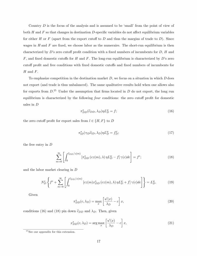
for exports from D.25 Under the assumption that firms located in D do not export, the long run

equilibrium is characterized by the following four conditions: the zero cutoff profit for domestic

sales in D

π∗DD(cDD, λD)ηLwD = f ; (16)

the zero cutoff profit for export sales from l ∈ {H,F} to D

π∗lD(τlD clD, λD)ηLwD = fxD; (17)

the free entry in D

∞∑m=0

[∫ cDD/z(m)

0[π∗DD (cz(m), λ) ηLwD − f ] γ(c)dc

]= fe; (18)

and the labor market clearing in D

N eD

{fe +

∞∑m=0

[∫ cDD/z(m)

0[cz(m)x∗DD (cz(m), λ) ηLwD + f ] γ(c)dc

]}= LwD. (19)

Given

π∗DD(c, λD) = maxx

[u′(x)

λD− c]x, (20)

conditions (16) and (18) pin down cDD and λD. Then, given

x∗DD(c, λD) = arg maxx

[u′(x)

λD− c]x, (21)

25See our appendix for this extension.

17

condition (19) pins down the number of entrants N eD and producers N

pD = Γ (cDD)N e

D.

The measure of products sold in D includes also those exported from l ∈ {H,F}. This is a

fraction Γ (clD) of the fixed measure of incumbent products Mil in l ∈ {H,F}:

NxlD = Γ (clD)M

il.

To determine clD, we write

π∗lD(τlDc, λD) = maxx

[u′(x)

λD− τlDc

]x (22)

and

x∗lD(τlDλDc) = arg maxx

[u′(x)

λD− τlDc

]x, (23)

with τlD > 1 . Then, given λD, condition (17) pins down clD. With fXD > f (17) also implies

τlD cHD < cDD.

Consider now the effects of raising η. By comparing the corresponding expressions in the closed

and the open economies, we see that all closed economy results fully apply to D variables (cDD, λD ,

N eD, N

pD) in the open economy. In particular, by (16) and (18), larger L

cD increases λD and decreases

cDD when the elasticity of inverse demand is increasing in consumption. Hence, accounting also

for the response of the export cutoff clD, the following result holds:

Proposition 2 (Open Economy) Consider an additive separable utility function satisfying (A1)-

(A2) and (B1-B3). Then a positive demand shock in an export market (i) increases the local

marginal utility of income, (ii) reduces the local firm cost cutoff, (iii) reallocates output, revenue

and employment from higher to lower cost exported products, and (iv) increases (decreases) profit

for low (high) exported cost products. Moreover, as long as the export fixed cost is large enough, the

positive demand shock also decreases the export cost cutoff and increases the number of exported

products, and aggregate exports.

Proof. See appendix.

When the fixed export cost is large enough, the demand shock in D has opposite effects on the

domestic cutoff (which increases) and the export cutoff (which decreases). This is due to the fact

that the demand shock, in equilibrium, induces a rotation of the residual demand curve faced by

18

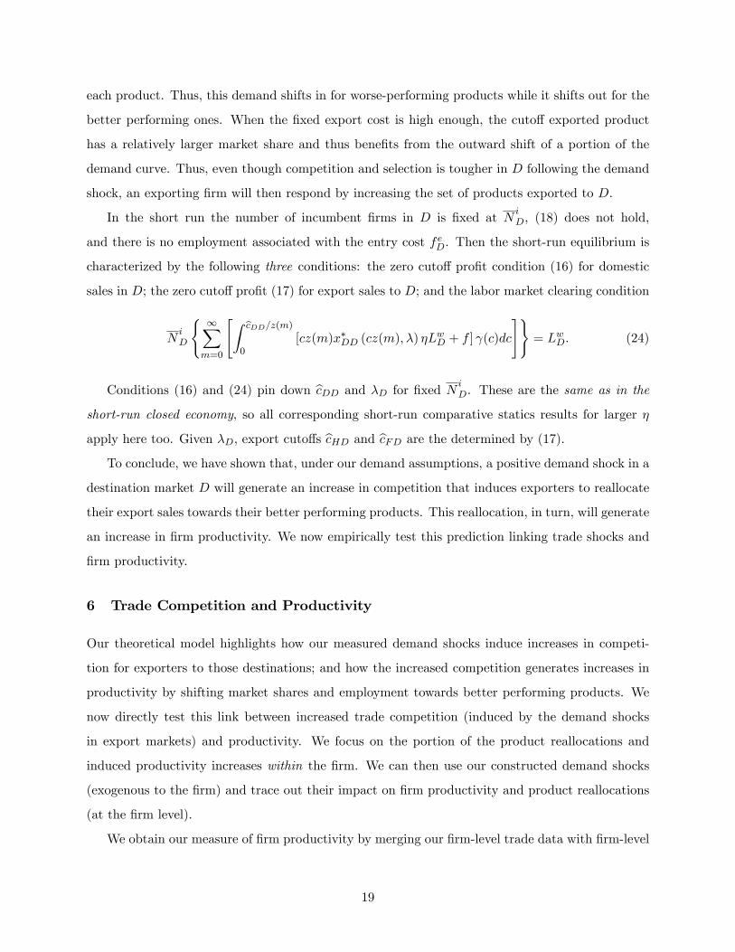
each product. Thus, this demand shifts in for worse-performing products while it shifts out for the

better performing ones. When the fixed export cost is high enough, the cutoff exported product

has a relatively larger market share and thus benefits from the outward shift of a portion of the

demand curve. Thus, even though competition and selection is tougher in D following the demand

shock, an exporting firm will then respond by increasing the set of products exported to D.

In the short run the number of incumbent firms in D is fixed at NiD, (18) does not hold,

and there is no employment associated with the entry cost feD. Then the short-run equilibrium is

characterized by the following three conditions: the zero cutoff profit condition (16) for domestic

sales in D; the zero cutoff profit (17) for export sales to D; and the labor market clearing condition

NiD

{ ∞∑m=0

[∫ cDD/z(m)

0[cz(m)x∗DD (cz(m), λ) ηLwD + f ] γ(c)dc

]}= LwD. (24)

Conditions (16) and (24) pin down cDD and λD for fixed NiD. These are the same as in the

short-run closed economy, so all corresponding short-run comparative statics results for larger η

apply here too. Given λD, export cutoffs cHD and cFD are the determined by (17).

To conclude, we have shown that, under our demand assumptions, a positive demand shock in a

destination market D will generate an increase in competition that induces exporters to reallocate

their export sales towards their better performing products. This reallocation, in turn, will generate

an increase in firm productivity. We now empirically test this prediction linking trade shocks and

firm productivity.

6 Trade Competition and Productivity

Our theoretical model highlights how our measured demand shocks induce increases in competi-

tion for exporters to those destinations; and how the increased competition generates increases in

productivity by shifting market shares and employment towards better performing products. We

now directly test this link between increased trade competition (induced by the demand shocks

in export markets) and productivity. We focus on the portion of the product reallocations and

induced productivity increases within the firm. We can then use our constructed demand shocks

(exogenous to the firm) and trace out their impact on firm productivity and product reallocations

(at the firm level).

We obtain our measure of firm productivity by merging our firm-level trade data with firm-level

19

production data. This latter dataset contains various measures of firm outputs and inputs. As

we are interested in picking up productivity fluctuations at a yearly frequency, we focus on labor

productivity measured as deflated value added per worker (using sector-specific price deflators).

We then separately control for the impact of changes in factor intensities and returns to scale (or

variable utilization of labor) on labor productivity. Note that this firm-level productivity measure

aggregates (using labor shares) to the overall deflated value-added per worker for manufacturing.

So long as our sector-specific price indices are accurately measured, this aggregate productivity

measure accurately tracks a welfare-relevant quantity index —even though we do not have access to

firm-level prices. In other words, the effect of pure markup changes at the sector level are netted-out

of our productivity measure. We can thus report a welfare-relevant aggregate productivity change

by aggregating our firm-level productivity changes using the observed changes in labor shares.26

6.1 Firm-Level Trade Shock

We cannot separately measure productivity at the destination or product level —only at the firm

level. We thus need to aggregate our destination-industry measures of demand shocks to the

firm-level. We use the firm’s market shares in those destinations and industries to perform this

aggregation.27 In a first step, we perform this aggregation over all export destinations and obtain

our firm-level demand shock in (log) levels and first difference:

shocki,t ≡∑d,I

xIi,d,t0xi,t0

× shockIi,d,t, ∆shocki,t =∑d,I

xIi,d,t−1

xi,t−1× ∆shockIi,d,t,

where xi,t ≡∑

d,I xIi,d,t represents firm i’s total exports in year t. As was the case for the construc-

tion of our firm-level destination shock (see 1), we only use the firm-level information on exported

products and market shares in prior years (the year of first export sales t0 for the demand shock in

levels and lagged year t−1 for the first difference between t and t−1). This ensures the exogeneity

of our constructed firm-level demand shocks (exogenous to firm-level actions in year t > t0 for

levels, and exogenous to firm-level changes ∆t for first differences). In particular, changes in the

26At the firm-level, an increase in markups across all products will be picked-up in our firm productivity measure—even though this does not reflect a welfare-relevant increase in output. But if this is the case, then this firm’s laborshare will decrease, and its productivity will carry a smaller weight in the aggregate index. In addition, increases infirm productivity are very strongly correlated with increases in labor shares —so this cannot be a pervasive componentof our measured productivity changes.27Later, when we focus on the impact of trade competition on skewness, we will show that those market shares are

the relevant weights to aggregate the destination-specific skewness measures.

20

set of exported products or exported market shares are not reflected in the demand shock.28

Ideally, this aggregation would also incorporate a firm’s exposure to demand shocks in its

domestic (French) market. This is not possible for two reasons: most importantly, we do not

observe the product-level breakdown of the firms’sales in the French market (we only observe total

domestic sales across products); in addition, world exports into France would not be exogenous to

firm-level technology changes in France. Therefore, we need to adjust our export-specific demand

shock using the firm’s export intensity to obtain an overall firm-level demand shock:

shock_intensi,t =xi,t0

xi,t0 + xi,F,t0shocki,t, ∆shock_intensi,t =

xi,t−1

xi,t−1 + xi,F,t−1∆shocki,t,

where xi,F,t denotes firm i’s total (across products) sales to the French domestic market in year

t (and the ratio thus measures firm i’s export intensity). Once again, we only use prior year’s

information on firm-level sales to construct this overall demand shock. Note that this adjustment

using export intensity is equivalent to assuming a demand shock of zero in the French market and

including that market in our aggregation by market share relative to total firm sales xi,t + xi,F,t.

6.2 Impact of the Trade Shock on Firm Productivity

In this section, we investigate the direct link between this firm-level demand shock and firm pro-

ductivity. Here, we focus exclusively on our firm-specific demand shock from (1), as this is our only

shock that exhibits firm-level variation within destinations. Our measure of productivity is the log

of deflated value-added per worker. In order to control for changes in capital intensity, we use the

log of capital per worker (Kit/Lit). We also control for unobserved changes in labor utilization and

returns to scale by using the log of raw materials (including energy use), Rit. Then, increases in

worker effort or higher returns to scale will be reflected in the impact of raw materials use on labor

productivity. As there is no issue with zeros for all these firm-level variables, we directly measure

the growth rate of those variable using simple first differences of the log levels.

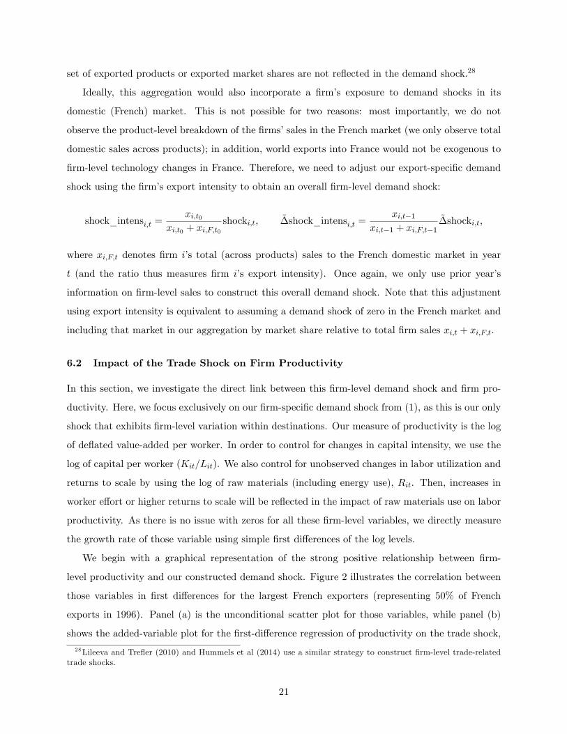
We begin with a graphical representation of the strong positive relationship between firm-

level productivity and our constructed demand shock. Figure 2 illustrates the correlation between

those variables in first differences for the largest French exporters (representing 50% of French

exports in 1996). Panel (a) is the unconditional scatter plot for those variables, while panel (b)

shows the added-variable plot for the first-difference regression of productivity on the trade shock,

28Lileeva and Trefler (2010) and Hummels et al (2014) use a similar strategy to construct firm-level trade-relatedtrade shocks.

21

with additional controls for capital intensity, raw materials (both in log first-differences) and time

dummies. Those figures clearly highlight the very strong positive response of the large exporters’

productivity to changes in trade competition in export markets (captured by the demand shock).

Figure 2: Exporters Representing 50% of French Trade in 1996: First Difference 1996-2005

-1.5

-1-.5

0.5

1 c

hang

e in

ln la

bour

pro

duct

ivity

-.2 -.1 0 .1 .2 change in ln trade shock

regression line: coef = .783, se = .198, N = 1063sample: 167 firms representing 50% of French exports in 1996

-1.5

-1-.5

0.5

1 c

ond.

cha

nge

in ln

labo

ur p

rodu

ctiv

ity

-.2 -.1 0 .1 .2cond. change in ln trade shock

regression line: coef = 1.094, se = .263, N = 1040sample: 167 firms representing 50% of French exports in 1996standard errors clustered by firm

(a) Unconditional (b) Conditional

Table 3 shows how this result generalizes to our full sample of firms and our three different

specifications (FE, FD, FD-FE). Our theoretical model emphasizes how a multi-product firm’s

productivity responds to the demand shock via its effect on competition and product reallocations

in the firm’s export markets. Thus, we assumed that the firm’s technology at the product level

(the marginal cost v(m, c) for each product m) was exogenous (in particular, in respect to demand

fluctuations in export markets). However, there is a substantial literature examining how this

technology responds to export market conditions via various forms of innovation or investment

choices made by the firm. We feel that the timing dimension of our first difference specifications —

especially our FD-FE specifications which nets out any firm-level growth trends —eliminates this

technology response channel: It is highly unlikely that a firm’s innovations or investment responses

to the trade shock in a given year (especially the innovation in the trade shock relative to trend)

would be reflected contemporaneously in the firm’s productivity. However, we will also show some

additional robustness checks that address this potential technology response.

The first three columns of Table 3 show that, across our three timing specifications, there is

22

a stable and very strong response of firm productivity to the trade shock. Since our measure

of productivity as value added per worker incorporates neither the impact of changes in input

intensities nor the effects of non-constant returns to scale, we directly control for these effects

in the next set of regressions. In the last 3 columns of Table 3, we add controls for capital per

worker and raw material use (including energy). Both of these controls are highly significant: not

surprisingly, increases in capital intensity are reflected in labor productivity; and we find that

increases in raw materials use are also associated with higher labor productivity. This would be

the case if there are increasing returns to scale in the value-added production function, or if labor

utilization/effort increases with scale (in the short-run). However, the very strong effect of the

trade shock on firm productivity remains when these controls are added —and they remain highly

significant, well beyond the 1% significance level. (From here on out, we will keep those controls in

all of our firm productivity regressions.)

Table 3: Baseline Resultsl: Impact of Trade Shock on Firm Productivity

Dependent Variable log prod. ∆ log prod. log prod. ∆ log prod.Specification FE FD FD-FE FE FD FD-FElog (trade shock × export intens.) 0.094a 0.073a

(0.019) (0.018)

∆ (trade shock × export intens.) 0.134a 0.116a 0.108a 0.096a

(0.024) (0.028) (0.024) (0.028)

log capital stock per worker 0.228a

(0.007)

log raw materials 0.091a

(0.004)

∆ log capital stock per worker 0.327a 0.358a

(0.008) (0.009)

∆ log raw materials 0.100a 0.093a

(0.004) (0.004)

Observations 213877 188328 188328 201627 174931 174931Standard errors (clustered at the firm level) in parentheses: c < 0.1, b < 0.05, a < 0.01

We now describe several robustness checks that further single-out our theoretical mechanism

operating through the demand-side product reallocations for multi-product firms. In the next table

we regress our capital intensity measure on our trade shock; the results in Table 4 show that there

23

is no response of investment to the trade shock. This represents another way to show that the

short-run timing for the demand shocks precludes a contemporaneous technology response: if this

were the case, we would expect to see some of this response reflected in higher investment (along

with other responses along the technology dimension).

Table 4: K/L Does Not respond to Trade Shocks

Dependent Variable ln K/L ∆ ln K/L ∆ ln K/LSpecification FE FD FD-FElog (trade shock × export intens.) -0.018

(0.018)

∆ (trade shock × export intens.) -0.003 -0.005(0.017) (0.020)

Observations 212745 186171 186171

Standard errors in parentheses: c < 0.1, b < 0.05, a < 0.01

Next we use a different strategy to control for the effects of non-constant returns to scale

or variable labor utilization: in Table 5, we split our sample between year intervals where firms

increase/decrease employment. If the effects of the trade shock on productivity were driven by scale

effects or higher labor utilization/effort, then we would expect to see the productivity responses

concentrated in the split of the sample where firms are expanding employment (and also expanding

more generally). Yet, Table 5 shows that this is not the case: the effect of the trade shock on

productivity is just as strong (even a bit stronger) in the sub-sample of years where firms are

decreasing employment; and in both cases, the coeffi cients have a similar magnitude to our baseline

results in Table 3.29

In order to further single-out our theoretical mechanism operating through the demand-side

product reallocations for multi-product firms, we now report two different types of falsification

tests. Our first test highlights that the link between productivity and the trade shocks is only

operative for multi-product firms. Table 6 reports the same regression (with controls) as our

baseline results from Table 3, but only for single-product exporters. This new table clearly shows

that this there is no evidence of this link among this subset of firms. Next, we show that this

productivity-trade link is only operative for firms with a substantial exposure to export markets

(measured by export intensity). Similarly to single-product firms, we would not expect to find a

29Since we are splitting our sample across firms, we no longer rely on the two specifications with firm fixed-effectsand only show results for the FD specification.

24

Table 5: Robustness to Scale Effects

Sample Employment Increase Employment DecreaseDependent Variable ∆ log productivity ∆ log productivitySpecification FD FD∆ (trade shock × export intens.) 0.135a 0.156a

(0.035) (0.045)

∆ log capital stock per worker 0.288a 0.332a

(0.012) (0.013)

∆ log raw materials 0.091a 0.097a

(0.005) (0.005)Observations 69642 65268

Standard errors in parentheses: c < 0.1, b < 0.05, a < 0.01

significant productivity-trade link among firms with very low export intensity. This is indeed the

case. In Table 7, we re-run our baseline specification using the trade shock before it is interacted

with export intensity. The first three columns report the results for the quartile of firms with the

lowest export intensity, and highlight that there is no evidence of the productivity-trade link for

those firms. On the other hand, we clearly see from the last three columns that this effect is very

strong and powerful for the quartile of firms with the highest export intensity.30

30Since the trade shock as not been interacted with export intensity, the coeffi cients for this top quartile representsignificantly higher magnitudes than the average coeffi cients across the whole sample reported in Table 3 (since exportintensity is always below 1). This is also confirmed by a specification with the interacted trade shock restricted tothis same top quartile of firms.

25

Table 6: Reduced Form: Single Product FirmsDependent Variable log prod. ∆ log prod.Specification FE FD FD-FElog (trade shock × export intens.) 0.005

(0.050)

log capital stock per worker 0.269a

(0.016)

log raw materials 0.101a

(0.010)

∆ (trade shock × export intens.) -0.021 -0.138c

(0.062) (0.079)

∆ log capital stock per worker 0.368a 0.415a

(0.020) (0.028)

∆ log raw materials 0.114a 0.090a

(0.010) (0.013)

Observations 32870 25330 25330Standard errors in parentheses: c < 0.1, b < 0.05, a < 0.01

26

Table 7: Reduced Form: Low/High export intensity

Sample exp. intens. quartile # 1 exp. intens. quartile # 4Dependent Variable log prod. ∆ log prod. log prod. ∆ log prod.Specification FE FD FD-FE FE FD FD-FElog trade shock 0.009 0.068a

(0.006) (0.014)

log capital stock per worker 0.278a 0.217a

(0.022) (0.015)

log raw materials 0.070a 0.128a

(0.006) (0.010)

∆ trade shock 0.000 -0.002 0.096a 0.100a

(0.007) (0.009) (0.017) (0.021)

∆ log capital stock per worker 0.323a 0.367a 0.325a 0.368a

(0.016) (0.020) (0.014) (0.016)

∆ log raw materials 0.070a 0.057a 0.129a 0.123a

(0.006) (0.006) (0.008) (0.010)

Observations 49227 38894 38894 53125 46347 46347Standard errors in parentheses: c < 0.1, b < 0.05, a < 0.01

27

7 Trade Competition and Product Reallocations at the Firm-Level

In order to further highlight the demand-side product reallocations channel for the productivity-

trade link, we now show that our trade shock aggregated to the firm level strongly predicts product

reallocations towards better performing products (higher market shares) at the firm level; that

is the firm’s global product mix (the distribution of product sales across all destinations). Our

theoretical model highlighted how (under our demand assumptions) those product reallocations

would then lead to higher firm productivity.

Our previous results highlighted how demand shocks lead to reallocations towards better per-

forming products at the destination-industry level. Intuitively, since there is a stable ranking of

products at the firm level (better performing products in one market are most likely to be the

better performing products in other markets —as we previously discussed), then reallocations to-

wards better performing products within destinations should also be reflected in the reallocations of

global sales/production towards better performing products; and the strength of this link between

the skewness of sales at the destination and global levels should depend on the importance of the

destination in the firm’s global sales. Our chosen measure of skewness, the Theil index, makes this

intuition precise. It is the only measure of skewness that exhibits a stable decomposition from the

skewness of global sales into the skewness of destination-level sales (see Jost 2007).31 Specifically,

let Ti,t be firm i’s Theil index for the skewness of its global exports by product xsi,t ≡∑

d xsi,d,t.

(the sum of exports for that product across all destinations).32 Then this global Theil can be

decomposed into a market-share weighted average of the within-destination Theils Ti,d,t and a

“between-destination” Theil index that measures differences in the distribution of product-level

market shares across destinations:33

Ti,t =∑d

xi,d,txi,t

Ti,d,t −∑d

xi,d,txi,t

TBi,d,t, (25)

31This decomposition property is similar —but not identical —to the within/between decomposition of Theil indicesacross populations. In the latter, the sample is split into subsamples. In our case, the same observation (in this case,product sales) is split into “destinations”and the global measure reflects the sum across “destinations”.32The Theil index is defined in the same way as the destination level Theil in (2).33For simplicity, we omit the industry referencing I for the destination Theils. The decomposition across industries

follows a similar pattern.

28

where the between-destination Theil TBi,d,t is defined as

TBi,d,t =∑s

xsi,d,txi,d,t

log

(xsi,d,t/xi,d,t

xsi,t/xi,t

).

Note that the weights used in this decomposition for both the within- and between-destination

Theils are the firm’s export shares xi,d,t/xi,t across destinations d. The between-destination Theil

TBi,d,t measures the deviation in a product’s market share in a destination d, xsi,d,t/xi,d,t, from that

product’s global market share xsi,t/xi,t and then averages these deviations across destinations. It is

positive and converges to zero as the distributions of product market shares in different destination

become increasingly similar.

To better understand the logic behind (25), note that it implies that the average of the within-

destination Theil indices can be decomposed into the sum of two positive elements: the global

Theil index, and the between-destination Theil index. This decomposition can be interpreted as

a decomposition of variance/dispersion. The dispersion observed in the destination level product

exports must be explained either by dispersion in global product exports (global Theil index), or

by the fact that the distribution of product sales varies across destinations (between-destination

Theil index).

A simple example helps to clarify this point. Take a firm with 2 products and 2 destinations.

In each destination, exports of one product are x, and exports of the other product are 2x. This

leads to the same value for the within-destination Theil indices of (1/3) ln (1/3) + (2/3) ln(2/3),

and hence the same value for the average within-destination Theil index. Hence, if the same

product is the better performing product in each market (with 2x exports), then the distributions

will be synchronized across destinations and the between-destination Theil will be zero: all of the

dispersion is explained by the global Theil index, whose value is equal to the common value of the

two within-destination Theil indices. On the other hand, if the opposite products perform better

in each market, global sales are 3x for each product. There is thus no variation in global product

sales, and the global Theil index is zero. Accordingly, all of the variation in the within-destination

Theil indices is explained by the between-destination Theil.

The theoretical model of Bernard, Redding and Schott (2011) with CES demand predicts that

the between-destination Theil index would be exactly zero when measured on a common set of

exported products across destinations. With linear demand, Mayer, Melitz and Ottaviano (2014)

show (theoretically and empirically) that this between-destination index would deviate from zero

29

because skewness varies across destinations. We have shown earlier that this result holds for

a larger class of demand systems such that the elasticity and the convexity of inverse demand

increase with consumption. Yet, even in these cases, the between-destination Theil is predicted to

be small because the ranking of the product sales is very stable across destinations. This leads to

a prediction that the market-share weighted average of the destination Theils should be strongly

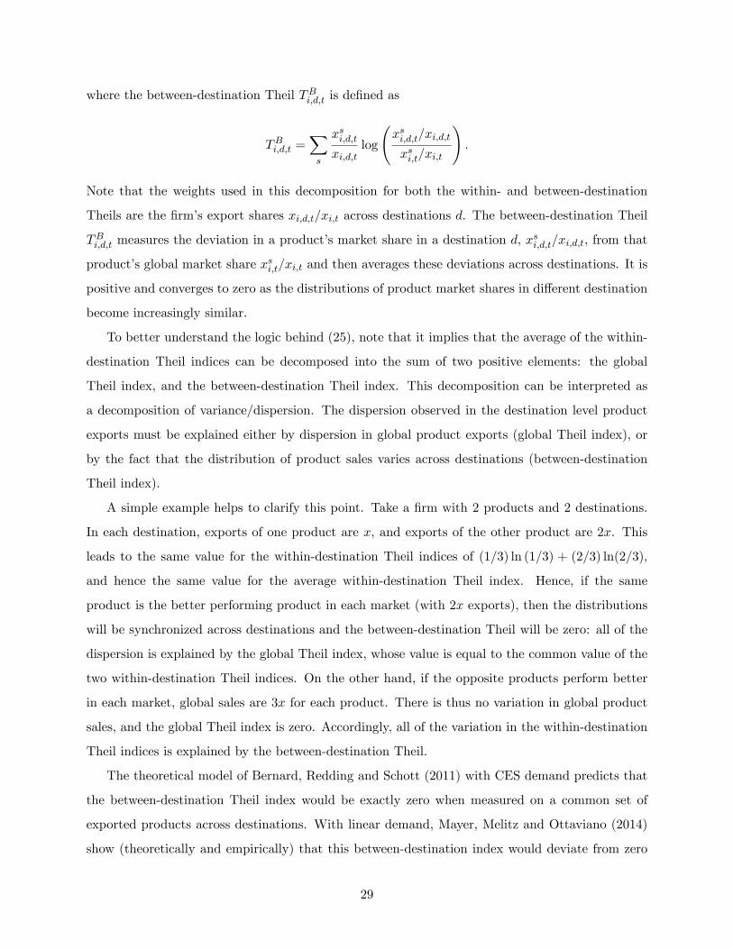
correlated with the firm’s global Theil. Empirically, this prediction is strongly confirmed as shown

in Figure 3.

Figure 3: Correlation Between Global Skewness and Average Local Skewness

This high correlation between destination and global skewness of product sales enables us to

move from our previous predictions for the effects of the trade shocks on skewness at the destination-

level to a new prediction at the firm-level. By aggregating the trade shocks across destinations

using the firm’s market share in each destination, we have constructed a firm-level trade shock that

predicts changes in the weighted average of destination skewness Ti,d,t —and hence will predict

changes in the firm’s global skewness Ti,t (given the high correlation between the two indices).

This result is confirmed by our regression of the firms’global Theil on our trade shock measures,

reported in the first three columns of Table 8. Our firm-level trade shock has a strong and highly

significant (again, well beyond the 1% significance level) impact on the skewness of global exports.

In this regression, we have also added back our two more aggregated measures of demand shocks:

the industry (ISIC-3) level trade shock and the GDP shock (aggregated to the firm-level using

the same market share weights across destinations). The industry level trade shock —which was

already substantially weaker than the firm-level trade shock in the destination-level regressions

30

— is no longer significant at the firm level. The GDP shock is not significant in the (log) levels

regressions, but is very strong and significant in the two first-difference specifications.

Table 8: The Impact of Demand Shocks on the Global Product Mix (Firm Level)

Dependent Variable Ti,t ∆Ti,t Exp. Intensi,t ∆ Exp. Intensi,tSpecification FE FD FD-FE FE FD FD-FElog GDP shock -0.001 0.003a

(0.004) (0.001)

log trade shock 0.045a 0.014a

(0.009) (0.003)

log trade shock - ISIC -0.001 0.000(0.001) (0.000)

∆ GDP shock 0.118a 0.107a 0.032a 0.035a

(0.031) (0.038) (0.010) (0.012)

∆ trade shock 0.057a 0.050a 0.019a 0.016a

(0.011) (0.013) (0.003) (0.004)

∆ trade shock - ISIC -0.003 -0.010 0.002 0.000(0.005) (0.007) (0.002) (0.002)

(0.110) (0.004) (0.004) (0.030) (0.001) (0.001)Observations 117851 117851 117851 110565 107283 107283

Standard errors in parentheses: c < 0.1, b < 0.05, a < 0.01

Our global Theil measure Ti,t measures the skewness of export sales across all destinations,

but it does not entirely reflect the skewness of production levels across the firm’s product range.

That is because we cannot measure the breakdown of product-level sales on the French domestic

market. Ultimately, it is the distribution of labor allocation across products (and the induced

distribution of production levels) that determines a firm’s labor productivity —conditional on its

technology (the production functions for each individual product). As highlighted by our theoretical

model, the export market demand shocks generate two different types of reallocations that both

contribute to an increased skewness of production levels for the firm: reallocations within the set of

exported products, which generate the increased skewness of global exports that we just discussed;

but also reallocations from non-exported products towards the better performing exported products

(including the extensive margin of newly exported products that we documented at the destination-

level). Although we cannot measure the domestic product-level sales, we can measure a single

31

statistic that reflects this reallocation from non-exported to exported goods: the firm’s export

intensity. We can thus test whether the firm-level trade shocks also induce an increase in the firm’s

export intensity. Those regressions are reported in the last three columns of Table 8, and confirm

that our firm-level trade shock has a very strong and highly significant positive impact on a firm’s

export intensity.34 The impact of the GDP coeffi cient is also strong and significant, whereas the

industry-level trade shock remains insignificant. Thus, our firm-level trade shock and GDP shock

both predict the two types of reallocations towards better performing products that we highlighted

in our theoretical model (as a response to increased competition in export markets). Holding the

firm’s product-level technology fixed, these reallocations both generate the subtantial increases in

firm-level productivity that we previously documented.

8 Can the Measured Product Reallocations Explain the Entire Impact of

Trade Competition on Productivity?

To be completed...

9 Conclusion

To be completed...

10 References

Arkolakis, Costas, Arnaud Costinot, Dave Donaldson and Andres Rodriguez-Clare. 2012. “The

Elusive Pro-Competitive Effects of Trade.”Unpublished, MIT.

Baldwin, John R. and Wulong Gu. 2009. “The Impact of Trade on Plant Scale, Production-Run

Length and Diversification.”In Producer Dynamics: New Evidence from Micro Data, edited

by T. Dunne, J.B. Jensen, and M.J. Roberts. Chicago: University of Chicago Press.

Berman, Nicolas, Philippe Martin, and Thierry Mayer. 2012. “How Do Different Exporters React

to Exchange Rate Changes?”Quarterly Journal of Economics 127 (1): 437-492.

Bernard, Andrew B., Stephen J. Redding and Peter K. Schott. 2011. “Multi-product Firms and

Trade Liberalization.”Quarterly Journal of Economics 126 (3): 1271-1318.

34Since the export intensity is a ratio, we do not apply a log-transformation to that variable. However, specificationsusing the log of export intensity yield very similar results.

32

Bernard, Andrew B., J. Bradford Jensen, Stephen J. Redding, and Peter K. Schott. 2012. “The

Empirics of Firm Heterogeneity and International Trade.”Annual Review of Economics 4

(1): 283—313.

Bernard, Andrew B., J. Bradford Jensen, Stephen J. Redding and Peter K. Schott. 2007. “Firms

in International Trade.”Journal of Economic Perspectives 21 (3): 105-130.

Bernard, Andrew.B., Jonathan Eaton, Brad Jensen, and Samuel Kortum. 2003. “Plants and

Productivity in International Trade.”American Economic Review 93 (4): 1268-1290.

De Loecker, Jan, Penny Goldberg, Amit Khandelwal and Nina Pavcnik. 2012. “Prices, Markups

and Trade Reform.” National Bureau of Economic Research, NBER Working Paper No.

17925.

Fabinger, Michal, and E. Glen Weyl. 2012. “Pass-Through and Demand Forms.”Unpublished,

University of Chicago.

Fabinger, Michal, and E. Glen Weyl (2014) “A Tractable Approach to Pass-Through Patterns

with Applications to International Trade,”University of Chicago.

Feenstra, Robert C. and David Weinstein. 2010. “Globalization, Markups, and the U.S. Price

Level.”NBER Working Paper 15749.

Harrison, Ann E.. 1994. “Productivity, Imperfect competition and trade reform : Theory and

evidence.”Journal of International Economics 36 (1-2): 53-73.

Hummels, David, Rasmus Jørgensen, Jakob Munch, and Chong Xiang. 2014. “The Wage Effects

of Offshoring: Evidence from Danish Matched Worker-Firm Data †.”American Economic

Review 104 (6): 1597—1629.

Iacovone, Leonardo and Beata S. Javorcik. 2008. “Multi-product Exporters: Diversification and

Micro-level Dynamics.”World Bank Working Paper No. 4723.

Levinsohn, James A.. 1993. “Testing the imports-as-market-discipline hypothesis.” Journal of

International Economics 35 (1-2): 1-22.

Lileeva, Alla, and Daniel Trefler. 2010. “Improved Access to Foreign Markets Raises Plant-Level

Productivity. . . For Some Plants.”The Quarterly Journal of Economics 125 (3): 1051—99.

33

Mayer, Thierry and Gianmarco I.P. Ottaviano. 2008. “The Happy Few: The Internationalisation

of European Firms.”Intereconomics 43 (3): 135-148.

Mayer, Thierry, Marc J. Melitz, and Gianmarco I.P. Ottaviano. 2014. “Market Size, Competition,

and the Product Mix of Exporters”, American Economic Review 104 (2): 495—536.

Melitz, Marc J. and Gianmarco I.P. Ottaviano. 2008. “Market Size, Trade and Productivity.”

Review of Economic Studies 75 (1): 295 -316.

Mrazova, Monika, and J. Peter Neary. 2014. “Not So Demanding: Preference Structure, Firm

Behavior, and Welfare.”Unpublished, Oxford University.

Parenti, Mathieu, Philip Ushchev and Jacques-François Thisse. 2014. “Toward a theory of mo-

nopolistic competition.”Unpublished, Université Catholique de Louvain.

Zhelobodko, Evgeny, Sergey Kokovin, Mathieu Parenti and Jacques-François Thisse. 2012. “Mo-

nopolistic Competition: Beyond the Constant Elasticity of Substitution.”Econometrica 80

(6): 2765-2784.

34

Appendix

A Higher cost is associated with higher price, lower output, lower revenue

and lower profit.

First, implicit differentiation of (4) yields

dxvdv

=λ

φ′(xv)< 0 (A.1)

where the sign is dictated by (A2). This shows that higher marginal cost leads to smaller output

qv = xvLv. Second, by (3), under (A1) smaller output implies higher price as

dpvdxv

=u′′(xv)

λ< 0

so higher marginal cost leads to higher price

dpvdv

=dpvdxv

dxvdv

=u′′(xv)

φ′(xv)> 0.

Third, given εp(xv) ∈ (0, 1), higher marginal cost is associated with lower revenue rvLv = pvxvLv

asdrvdv

=dpvxvdv

= [1− εp(xv)]dxvdv

< 0

which shows that the negative effect of cost on output dominates its positive effect on price. Fourth,

by the envelope theorem, also profit is a decreasing function of marginal cost as

dπvdv

= −xv < 0 (A.2)

where πv = (pv − v)xvLc is operating profit. Hence, (A1) and (A2) are necessary and suffi cient for

higher cost products to associated with higher price, lower output, lower revenue and lower profit.

B Lower cost is associated with higher markup

From (5), the (multiplicative) markup equals

mv =pvv

=1

1− εp(xv)(B.1)

35

Given that in (a) we have already shown that xv is a decreasing function of v, markup mv will

be decreasing or increasing in v depending on whether the elasticity of inverse demand ε′p(xv) is

positive or negative. Moreover, that ε′p(xv) R 0 is equivalent to εr(xv) R εp(xv) can be seen by

noting that we can writeε′p(xv)xv

εp(xv)=

1− εp(xv)εp(xv)

[εr(xv)− εp(xv)]

so that, given εp(xv) ∈ (0, 1), ε′p(xv) R 0 if and only if εr(xv) R εp(xv).

Arkolakis, Costinot, Donaldson and Rodriguez-Clare (2012) assume that demand functions are

log-concave in log-prices for all differentiated goods (this is their assumption "A3"). To compare

(B1) with this assumption, invert our inverse demand

pi =u′(xi)

λ, with λ =

∫ M

0u′(xi)xidi

to obtain (direct) demand

xi = u′−1(eln pi+lnλ

). (B.2)

Then, define the function

d(y) = u′−1 (ey)

and rewrite (B.2) as

xi = d(ln pi + lnλ)

This is the way Arkolakis, Costinot, Donaldson and Rodriguez-Clare (2012) state their demand

system in the separable case. Clearly, under (A1) d(y) is strictly decreasing so that we have

d′(y) < 0. Arkolakis, Costinot, Donaldson and Rodriguez-Clare (2012) define “log-concavity”as

d′′(y) < 0

i.e. d′′(y) is concave. As the inverse of a strictly decreasing strictly concave real function is strictly

concave, strict concavity of d(y) implies strict concavity of its inverse

yi = lnu′(xi).

36

The concavity of this function depends on the sign of its second derivative

d2 lnu′(xi)

dx2i

=u′′′(xi)u′(xi)− u′′(xi)u′′(xi)

[u′(xi)]2 ,

which, under (A1), is negative if and only if

u′′′(xi)xiu′′(xi)

− u′′(xi)xiu′(xi)

> 0

or equivalentlyεr(xv)

εp(xv)>

2− εp(xv)1− εp(xv)

As the term on the right hand side is larger than one, the assumption of “log-concavity” in the

sense of Arkolakis, Costinot, Donaldson and Rodriguez-Clare (2012) is more restrictive than our

assumption (B1).

C Pass-through is incomplete and lower cost is associated smaller

pass-through

Define the pass-through as

θ(xv) ≡d ln p(xv)

d ln v=d ln p(xv)

d lnxv

d lnxvd ln v

By definition we haved ln p(xv)

d lnxv= −εp(xv)

while implicit differentiation of (3) gives

dxvdv

=λ

φ′(xv)

so thatd lnxvd ln v

=φ(xv)

φ′(xv)xv= − 1

εr(xv)

where the first equality is granted by (3) and the second equality is granted by definition. Accord-

ingly, the pass-through can be expressed as

θ(xv) =εp(xv)

εr(xv)(C.1)

37

with θ(xv) < 1 when (B1) holds. Differentiating (C.1) show that

ε′p(xv)xv

εp(xv)<ε′r(xv)xvεr(xv)

is necessary and suffi cient for θ′(xv) < 0. Then, given (B1) ε′p(xv) > 0, ε′r(xv) > 0 is necessary for

θ′(xv) < 0.

In Berman, Martin and Mayer (2102) an exporter to destination market D maximizes

maxqi≥0

πD(qi) =piεDqi − vqi − f

subject to

pi =u′(xi)

λ, with λ =

∫ M

0u′(xi)xidi

where pi is the price denominated in the destination’s currency, v is the marginal cost denominated

in the currency of the firm’s country, and εD is the exchange rate. The FOC for profit maximization

is

u′(xi) + u′′(xi)xi = ελc

which implies that the pass-through from marginal cost to price is homomorphic to the pass-through

from exchange rate to price.

D Lower cost is associated with larger employment

Employment in the supply of a product with marginal cost v equals vxvLc. Differentiation yields

dvxvdv

=

(1 +

∂xv∂v

v

xv

)xv =

(1− 1

εr(xv)

)xv

where the second equality is granted by (3) together with the definitions of εp(xv) and εr(xv).

Hence, employment decreases with marginal cost if and only if εr(xv) < 1.

E Long-Run Response to a Demand Shock in Closed Economy (Proposition 1)

The effects of a demand shock on c∗ and λ can be characterized extending the analysis by Zhelo-

bodko et al (2012) to the case of multiproduct firms. The reason is that, as these effects are fully

determined by (11) and (12), changing η is paramount to changing Lc, which is the comparative

38

statics experiment studied by Zhelobodko et al (2012).

Too see this, rewrite expressions (10) in terms of elasticities as

επ∗/λ(λv) =∂π∗(v, λ)

∂λ

λ

π∗(v, λ)= − 1

1− cu′(x∗(λv))

λ

= − 1

εp(x∗(λv))(E.1)

επ∗/v(λv) = −∂π∗(v, λ)

∂v

v

π∗(v, λ)= − v

p(x∗(λv))− v = −1− εp(x∗(λv))

εp(x∗(λv))(E.2)

To obtain dλ∗/dLc > 0 divide (12) by Lc to yield

∞∑m=0

∫ c/z(m)

0π∗ (cz(m), λ) γ(c)dc =

feLc

+f

Lc

∞∑m=0

Γ

(c

z(m)

)(E.3)

where regularity conditions are assumed on z(m) to make the series on the right hand side converge.

Then differentiate with respect to Lc to get

∂λ

∂Lc

∞∑m=0

∫ c/z(m)

0

∂π∗ (cz(m), λ)

∂λγ(c)dc+

∂c

∂Lc

∞∑m=0

π∗ (c, λ)γ(c/z(m))

z(m)

= − fe

(Lc)2 −f

(Lc)2

∞∑m=0

Γ

(c

z(m)

)+

∂c

∂Lcf

Lc

∞∑m=0

γ (c/z(m))

z(m)

∂λ

∂Lc

∞∑m=0

∫ c/z(m)

0

∂π∗ (cz(m), λ)

∂λγ(c)dc+

∂c

∂Lc

∞∑m=0

[π∗ (c, λ)− f

Lc

]γ(c/z(m))

z(m)(E.4)

= − fe

(Lc)2 −f

(Lc)2

∞∑m=0

Γ

(c

z(m)

)

By (11), the term between square brackets equals zero while again (12) implies

− fe

(Lc)2 −f

(Lc)2

∞∑m=0

Γ

(c

z(m)

)= −

∑∞m=0

∫ c/z(m)0 π∗ (cz(m), λ) γ(c)dc

Lc

Exploiting these results, (E.4) can be restated in terms of elasticities as

∂λ

∂Lc

∞∑m=0

∫ c/z(m)

0

∂π∗ (cz(m), λ)

∂λγ(c)dc = −

∑∞m=0

∫ c/z(m)0 π∗ (cz(m), λ) γ(c)dc

Lc

39

∂λ

∂LcLc

λ

∞∑m=0

∫ c/z(m)

0

∂π∗ (cz(m), λ)

∂λ

λ

π∗ (cz(m), λ)π∗ (cz(m), λ) γ(c)dc

= −∞∑m=0

∫ c/z(m)

0π∗ (cz(m), λ) γ(c)dc

ελ/Lc(λc)∞∑m=0

∫ c/z(m)

0επ∗/λπ

∗ (cz(m), λ) γ(c)dc = −∞∑m=0

∫ c/z(m)

0π∗ (cz(m), λ) γ(c)dc

ελ/Lc(λc) = −∑∞

m=0

∫ c/z(m)0 π∗ (cz(m), λ) γ(c)dc∑∞

m=0

∫ c/z(m)0 π∗ (cz(m), λ) επ∗/λγ(c)dc

=

∑∞m=0

∫ c/z(m)0 π∗ (cz(m), λ) γ(c)dc∑∞

m=0

∫ c/z(m)0

π∗(cz(m),λ)εp(x∗(λcz(m)))γ(c)dc

(E.5)

where the last equality is granted by (E.1). The restriction εp(x∗(λv)) ∈ (0, 1) implies ελ/Lc ∈ (0, 1).

This proves point (i) in the proposition.

To determine the sign of εc/Lc(λc), differentiate (11) with respect to Lc and get

∂π∗(c, λ)

∂c

∂c

∂Lc+∂π∗(c, λ)

∂λ

∂λ

∂Lc= − f

(Lc)2 = −π∗(c, λ)

Lc

where the last equality is also granted by (11), or in terms of elasticities

επ∗/cεc/Lc + επ∗/λελ/Lc = −1

After substituting for (E.1), (E.2) and (E.5), this equation can be solved for εc/Lc to yield

εc/Lc(λc) =εp(x

∗(λc))− ελ/Lc1− εp(x∗(λc))

=εp(x

∗(λc))

1− εp(x∗(λc))

1−∑∞

m=0

∫ c/z(m)0

π∗(cz(m),λ)εp(x∗(λc)) γ(c)dc∑∞

m=0

∫ c/z(m)0

π∗(cz(m),λ)εp(x∗(λcz(m)))γ(c)dc

The sign of this expression is dictated by the sign of the term in square brackets given εp(x∗(λv)) ∈

(0, 1). As x∗(λv) > x∗(λc) for all v < c, then εp(x∗(λv)) > εp(x

∗(λc)) for all v < c when

ε′p(x∗(λc)) > 0. In this case, εc/Lc(λc) < 0 follows. Vice versa, εc/Lc(λc) > 0 follows from

ε′p(x∗(λc)) < 0. This proves that larger Lc = ηLw reduces (increases) the cost cutoff when the

elasticity of inverse demand is increasing in consumption, i.e. when (B1) holds. This proves point

(ii) in the proposition.

The effects of a demand shock on intensive margin reallocations can be assessed as follows.

Start with point (iii) in the proposition. By result (e), larger Lc = ηLw increases the marginal

utility of income λ. Hence, the impact of larger ηLw on output, revenue and employment ratios

has the same sign as the impact of λ on them.

40

Consider first the impact on the output ratio xv/xv:

d(xvxv

)dλ

=

dxvdλ xv − xv

dxvdλ

(xv)2

The sign of the right hand side is dictated by the numerator. Implicit differentiation of (4) can be

used to substitute for dxc/dλ and dxv/dλ, rewriting the numerator first as

cφ(xv)

φ′(xv)xc

φ(xv)

−v

φ(xv)xv

φ(xv)φ′(xv)

and then, using (4) and the definition of the elasticity of marginal revenue in (8), as

εr(xv)− εr(xv).

Repeating the same argument for any pair of values xv and xv such that xv > xv implies that

d(xv/xv

)/dλ > 0 as long as ε′r(xv) > 0, which is the case under (B2).

Consider now impact on the revenue ratio

d(rv/rv

)dλ

λ

rv/rv=∂rv∂xv

∂xv∂λ

λ

rv− ∂rv∂xv

∂xv∂λ

λ

rv= εr(xv)

λ

rv− εr(xv)

λ

rv

By result (a), we have xv > xv and rv > rv. Then, ε′r(xv) > 0 implies d(rv/rv

)/dλ > 0.

Last, consider the impact on the employment ratio. Larger λ implies a reallocation from the

higher to lower cost products when vxv/vxv > 1 and d(vxv/vxv

)/dλ > 0. By result (d), the

employment ratio is larger than one under (B3) εr(xv < 1. Moreover, as v and v are given, the

employment ratio increases with λ when the output ratio increases in λ, that is, when ε′r(xv) > 0,

which is again the case under (B2).

Finally, consider point (iv) in the proposition. To see how changes in η affect π∗(v, λ)Lc,

differentiate to obtain

∂π∗(v, λ)Lc

∂Lc= π∗(v, λ) +

∂π∗(v, λ)

∂λ

∂λ

∂LcLc

= π∗(v, λ)

(1 +

∂π∗(v, λ)

∂λ

λ

π∗(v, λ)

∂λ

∂LcLc

λ

)= π∗(v, λ)

(1 + επ∗/λ(λv)ελ/Lc(λc)

)

41

which can be rewritten as

∂π∗(v, λ)Lc

∂LcLc

π∗(v, λ)Lc= 1 + επ∗/λ(λv)ελ/Lc(λc)

and thus as

επ∗Lc/Lc(v, λ, c) = 1 + επ∗/λ(λv)ελ/Lc(λc) (E.6)

where ελ/Lc(λc) is common across products while επ∗/λ(λc) is product-specific and is given by (E.1)

both in the short and in the long run. By (E.1), expression (E.6) can be restated as

επ∗Lc/Lc(v, λ, c) = 1−ελ/Lc(λc)

εp(x∗(λv))

with εp(x∗(λv)) ∈ (0, 1). In the long run, by (E.5), we also have ελ/Lc(λc) ∈ (0, 1) so that π∗(v, λ)Lc

increases (decreases) with Lc for low v and decreases (increases) with λ for high v as long as

ε′p(xv) > (<)0. In the short run, the same results hold when the change in Lc is driven by η (as

∂λ/∂η > 0 implies ελ/Lc(λc) > 0).

F A positive demand shock increases the productivity of multi-product firms

By result (d), larger λ increases the employment ratio `m/`m′ of a lower cost product m to a higher

cost one m′. As the employment ratio equals the employment share ratio

`m`m′

=

`m∑M−1m=0 `m

`m′∑M−1m=0 `m

=smsm′

,

by increasing `m/`m′ , larger λ also increases sm relative to sm′ for any m < m′. Given that pro-

ductivity levels 1/vm’s are fixed, a higher share ratio in turn implies that larger λ increases average

productivity as this is an average in which the weighting is being shifted from lower productivity

(higher cost) products like m′ towards higher productivity (lower cost) products like m.35

35Everything would hold weakly if we relaxed the ranking condition v0 < v1 < ... < vM−1 to v0 ≤ v1 ≤ ... ≤ vM−1.

42

G Short-Run Response to a Demand Shock in Closed Economy

To see what happens when η changes in the short run, differentiate (11) to yield

∂π∗(c, λ)

∂λ

∂λ

∂η+∂π∗(c, λ)

∂c

∂c

∂η= − f

η2Lw

Then rewrite (15) as

∞∑m=0

∫ c/z(m)

0cz(m)x∗ (cz(m), λ) γ(c)dc =

1

ηN− f

ηLw

∞∑m=0

Γ(c/z(m))

and differentiate to obtain[ ∞∑m=0

∫ c/z(m)

0cz(m)

∂x∗ (cz(m), λ)

∂λγ(c)dc

]∂λ

∂η+

∞∑m=0

[(cx∗ (c, λ) +

f

ηLw

)γ(c/z(m))

z(m)

]∂c

∂η

= −Lw − fN

∑∞m=0 Γ(c/z(m))

η2LwN< 0

where the negative sign is due to the fact that Lw − fN∑∞

m=0 Γ(c/z(m)) > 0 is labor absorbed by

variable production costs. In matrix notation we can rewrite

∂π∗(c,λ)∂λ

∂π∗(c,λ)∂c∫ c

o c∂x∗(λc)∂λ γ(c)dc

∑∞m=0

[(cx∗ (c, λ) + f

ηLw

)γ(c/z(m))z(m)

] ∂λ

∂η

∂c∂η

=

− f

η(Lw)2

−Lw−fN∑∞m=0 Γ(c/z(m))

η2LwN

which can be solved by Cramer rule to obtain

∂λ

∂η=− f

η(Lw)2

[∑∞m=0

(cx∗ (c, λ) + f

ηLw

)γ(c/z(m))z(m)

]γ(c) +

Lw−fN∑∞m=0 Γ(c/z(m))

η2LwN

∂π∗(c,g)∂c

∂π∗(c,λ)∂λ

[∑∞m=0

(cx∗ (c, λ) + f

ηLw

)γ(c/z(m))z(m)

]− ∂π∗(c,λ)

∂c

∫ co c

∂x∗(λc)∂λ γ(c)dc

> 0

and

∂c

∂η=

−Lw−fN∑∞m=0 Γ(c/z(m))

η2LwN

∂π∗(c,λ)∂λ + f

η(Lw)2

[∫ co c

∂x∗(λc)∂λ γ(c)dc

]∂π∗(c,λ)∂λ

[∑∞m=0

(cx∗ (c, λ) + f

ηLw

)γ(c/z(m))z(m)

]− ∂π∗(c,λ)

∂c

∫ co c

∂x∗(λc)∂λ γ(c)dc

T 0

where the sign of ∂λ/∂η is dictated by (9) and (10), while the sign of ∂c/∂η depends on distributional

assumptions. The fact that the sign of ∂λ/∂η is positive while the sign of ∂c/∂η is ambiguous implies

that result (f) as well as all results in Proposition 1 except (ii) also hold in the short run.

43

H Response to a Demand Shock in Open Economy

To see what happens to the export cutoff when LcD changes due to changing η, rewrite (17) as

π∗lD(τlD clD, λD) =fxDηLcD

with l ∈ {H,F}. Differentiation with respect to LcD gives

∂π∗lD(τlD clD, λD)

∂clD

∂clD∂LcD

+∂π∗lD(τlD clD, λD)

∂λD

∂λD∂LcD

= − fxD(LcD)2

which can be restated as

∂clD∂LcD

=

−∂π∗lD(τlD clD,λD)∂λD

∂λD∂LcD− fxD

(LcD)2

∂π∗lD(τlD clD,λD)

∂clD

Given ∂π∗lD/∂λD < 0, ∂π∗lD/∂clD < 0 (as π∗(v, λ) is a decreasing function of v) and ∂λD/∂LcD > 0

when (A1)-(A2) hold, the export cutoff increases with LcD as long as fxD is large enough. Hence, as

η rises, smaller cDD for ε′p(xc) > 0 is accompanied by larger clD for large enough fxD. This leads to

a larger number of exported products MxlD = Γ (clD)M

il.

Aggregate exports from country l ∈ {H,F} are

EXPlD = Nil

∞∑m=0

[∫ clD/z(m)

0[x∗lD (cz(m), λ)LcD + f ] γ(c)dc

]

where Nil is the fixed measure of incumbent firms in l. Dividing by N

il and diffentiating gives

1

Nil

∂EXPlD∂LcD

=

{ ∞∑m=0

[∫ clD/z(m)

0

∂x∗lD (cz(m), λ)

∂λDLcDγ(c)dc

]}∂λD∂LcD

+

∞∑m=0

[∫ clD/z(m)

0x∗lD (cz(m), λ) γ(c)dc

]

+

{ ∞∑m=0

[x∗lD (clD, λ)LcD + f ]γ(clD/z(m))

z(m)

}∂clD∂LcD

Given ∂π∗lD/∂λD < 0 and ∂λD/∂LcD > 0 when (A1)-(A2) hold, the first term on the right hand

side is negative. Hence, we get ∂EXPlD/∂LcD > 0 as long as fxD is large enough to make ∂clD/∂LcD

positive and large enough.

44

I Allowing for the Destination Country to Export

In the main text we have analyzed a situation in which D does not export. This assumption is not

crucial, either in the long or the short run. Consider the long run. With exports from D the free

entry condition would become

fe =∞∑m=0

[∫ cDD/z(m)

0[π∗DD (cz(m), λ) ηLwD − f ] γ(c)dc

]

+

∞∑m=0

[∫ cDH/z(m)

0[π∗DH (cz(m), λ) ηLwH − fxH ] γ(c)dc

]

+∞∑m=0

[∫ cDF /z(m)

0[π∗DF (cz(m), λ) ηLwF − fxF ] γ(c)dc

]

where the second and third terms on the right hand side are constant for our comparative statics

analysis with respect to η. In particular, comparison with (18) reveals that allowing for exports

from D is homomorphic to reducing the entry cost feD to

feD−∞∑m=0

{∫ cDH/z(m)

0[π∗DH (cz(m), λ) ηLwH − fxH ] γ(c)dc+

∫ cDF /z(m)

0[π∗DF (cz(m), λ) ηLwF − fxF ] γ(c)dc

}.

The assumption of D not exporting is also not crucial in the short run. With exports from D

the labor market clearing condition would become

LwD = NiD

{fe +

∞∑m=0

[∫ cDD/z(m)

0[cz(m)x∗DD (cz(m), λ) ηLwD + f ] γ(c)dc

]

+∞∑m=0

[∫ cDH/z(m)

0[cz(m)x∗DH (cz(m), λ) ηLwH + fxH ] γ(c)dc

]

+

∞∑m=0

[∫ cDF /z(m)

0[cz(m)x∗DF (cz(m), λ) ηLwF + fxF ] γ(c)dc

]}

where the second and third terms on the right hand side are again constant for our comparative

statics analysis with respect to η. In particular, as comparison with (19) and (24) reveals, by

introducing another fixed source of employment for D’s workers, allowing for exports from D is

45

homomorphic to introducing some sort of fictitious ‘entry cost’

feD? ≡∞∑m=0

[∫ cDH/z(m)

0[cz(m)x∗DH (cz(m), λ) ηLwH + fxH ] γ(c)dc

+

∫ cDF /z(m)

0[cz(m)x∗DF (cz(m), λ) ηLwF + fxF ] γ(c)dc

]

also in the short run.

46