process integration study for increased energy efficiency...
TRANSCRIPT
Process integration study for increased
energy efficiency of a PVC plant
Master’s Thesis within the Sustainable Energy Systems programme
ÅSA LINDQVIST Department of Energy and Environment Division of Heat and Power Technology CHALMERS UNIVERSITY OF TECHNOLOGY Göteborg, Sweden 2011

MASTER’S THESIS
Process integration study for increased
energy efficiency of a PVC plant
Master’s Thesis within the Sustainable Energy Systems programme
ÅSA LINDQVIST
SUPERVISORS:
Roman Hackl
Kent Olsson
EXAMINER
Professor Simon Harvey
Department of Energy and Environment Division of Heat and Power Technology
CHALMERS UNIVERSITY OF TECHNOLOGY
Göteborg, Sweden 2011
Process integration study for increased energy efficiency of a PVC plant Master’s Thesis within the Sustainable Energy Systems programme ÅSA LINDQVIST
© ÅSA LINDQVIST, 2011
Department of Energy and Environment Division of Heat and Power Technology Chalmers University of Technology SE-412 96 Göteborg Sweden Telephone: + 46 (0)31-772 1000 Cover: INEOS’ PVC production site in Stenungsund. Chalmers Reproservice Göteborg, Sweden 2011

I
Process integration study for increased energy efficiency of a PVC plant Master’s Thesis within the Sustainable Energy Systems programme ÅSA LINDQVIST Department of Energy and Environment Division of Heat and Power Technology Chalmers University of Technology
ABSTRACT
Increasing energy prices combined with the need to reduce greenhouse gas emissions makes energy efficiency important both for economical and environmental reasons. In the energy-intensive industry, such as the process industry, there is a substantial potential for energy savings. INEOS ChlorVinyls, a major chlor-alkali producer, has a PVC production site in Stenungsund, on the West coast of Sweden. The site is a large consumer of both electricity and different fuels, and it is therefore relevant to perform a systematic energy efficiency study of the site.
This master’s thesis has investigated the possibilities for increasing the energy efficiency of INEOS’ PVC production site by increased internal heat recovery. The production of PVC is divided into three sub-processes. In this study focus has been on the second sub-process, which is the VCM production plant. Since the site is to be retrofitted in a near future, and the production capacity will be extended, the study was made for a future scenario with increased production. To identify options for increasing the energy efficiency of the site, pinch analysis has been used. Pinch analysis is a systematic method for identifying opportunities for improving the integration of processes in order to decrease the amount of external heating and cooling needed.
The results show that theoretically 7.8 MW of steam and the same amount of cooling water could be saved by internal heat exchange in the future VCM plant. This corresponds to 37% of the steam use. The pinch violations in the heat exchanger network were identified, and different retrofits are proposed, aiming to eliminate the five largest pinch violations in the system. Both direct heat transfer and the use of a heat transfer media such as water have been investigated. The suggested retrofits lead to steam savings between 4.5 and 6.5 MW, and an economic evaluation shows that the annual savings could reach 20 MSEK with a short pay-back period of about one year. Both in the existing and future VCM-plant, there is a large excess of low-grade heat below the pinch, which could be used for heating at other parts of the site. This would enable additional steam savings of the same size as in the proposed retrofits for increased internal heat transfer.
Key words: PVC plant, VCM plant, Energy efficiency, Pinch analysis

II
Studie av processintegration för ökad energieffektivitet i en PVC-anläggning Examensarbete inom masterprogrammet Sustainable Energy Systems ÅSA LINDQVIST Institutionen för Energi och Miljö Avdelningen för Värmeteknik och maskinlära Chalmers tekniska högskola
SAMMANFATTNING
Stigande energipriser tillsammans med behovet av att minska utsläppen av växthusgaser gör energieffektivisering mycket viktigt, både av ekonomiska och miljömässiga skäl. Inom den energiintensiva industrin, exempelvis processindustrin, finns en avsevärd potential för energibesparing. INEOS ChlorVinyls, en stor kloralkaliproducent, har en PVC-produktionsanläggning i Stenungsund på Sveriges västkust. Anläggningen förbrukar stora mängder av både el och olika bränslen, och det finns därför anledning att utföra en systematisk energieffektivitetsanalys av anläggningen.
Detta examensarbete har undersökt möjligheterna att öka energieffektiviteten för INEOS anläggning genom ökad intern värmeåtervinning. Produktionen av PVC är uppdelad i tre delsteg. Denna studie har fokuserat på VCM-fabriken, som är produktionens andra steg. Eftersom delar av anläggningen kommer att byggas ut inom en snar framtid, och produktionskapaciteten kommer att utökas, är studien gjord för ett framtida scenario med ökad produktion. För att hitta möjliga energieffektiviseringsåtgärder har pinchanalys använts. Pinchanalys är en systematisk metod för att hitta möjligheter för förbättrad processintegration, med syfte att minska mängden extern värme och kyla.
Resultaten visar att 7.8 MW ånga och lika mycket kylvatten teoretiskt kan sparas genom ökad intern värmeväxling i den framtida VCM-fabriken. Det motsvarar 37 % av ångbehovet. Pinchbrotten i värmeväxlarnätverket har identifierats, och olika förbättringsförslag har undersökts, med målet att eliminera de fem största pinchbrotten i systemet. Både direktvärmeväxling och användning av ett värmeöverföringsmedium, såsom vatten, har undersökts. De föreslagna åtgärderna ger ångbesparingar på mellan 4.5 och 6.5 MW, och en ekonomisk utvärdering visade att de årliga besparingarna kunde uppgå till 20 miljoner kronor för åtgärder med en kort återbetalningstid på ca ett år. I VCM-fabriken finns ett stort värmeöverskott under pinchtemperaturen, vilket skulle kunna användas i andra delar av anläggningen. Det skulle kunna möjliggöra ytterligare ångbesparingar av samma storleksordning som de föreslagna åtgärderna för värmeväxling.
Nyckelord: PVC, VCM, energieffektivitet, pinchanalys

III
Contents
ABSTRACT I
SAMMANFATTNING II
CONTENTS III
PREFACE V
NOTATIONS VII
1 INTRODUCTION 1
1.1 Purpose and objective 2
2 PROCESS DESCRIPTION 3
2.1 Process overview 4
2.1.1 The chlorine plant 5
2.1.2 The VCM plant 6
2.1.3 The PVC plant 6
2.2 Detailed description of the VCM plant 7
2.2.1 The HTC unit 7
2.2.2 The VCM unit 9
2.2.3 The OXI unit 10
2.2.4 The EDC-cleaning unit 12
2.3 Assumptions about the future VCM plant 13
3 METHODOLOGY 15
3.1 Data extraction 15
3.2 Aspen simulations 15
3.3 Pinch analysis 16
3.4 CO2 emissions evaluation 19
3.5 Economic evaluation 21
3.5.1 Investment costs 21
3.5.2 Annual savings 23
3.5.3 Payback time 23
4 RESULTS 25
4.1 System definition and process heating and cooling requirements 25
4.2 Pinch analysis of the future VCM plant 27
4.2.1 Possible measures for increased energy efficiency 29
4.3 Pinch violations in the VCM plant 30
4.4 Proposed measures for increased internal heat transfer in the future VCM plant 32
4.4.1 Retrofit 1 34
IV
4.4.2 Retrofit 2 36
4.4.3 Retrofit 3 37
4.4.4 Evaluation of the retrofits 38
4.5 Hot water system and steam production instead of direct heat exchange in the future VCM plant 40
4.5.1 Proposed retrofits, using hot water systems 42
4.5.2 Possibilities for low-pressure steam production 45
4.6 Use of excess heat from the VCM plant in the PVC plant 46
4.7 Heat from flue gases and Oxi-reactors 49
4.8 Uncertainties about the results 51
5 DISCUSSION 53
5.1 Cooling water and 1-barg steam 53
5.2 Carbon dioxide emissions price 53
5.3 Other possibilities 53
5.4 Advantages/disadvantages with hot water production and steam production instead of direct heat transfer 54
5.5 Other comments 54
6 CONCLUSIONS 57
7 FUTURE WORK 59
8 REFERENCES 61
9 APPENDIX 63

V
Preface
In this Master’s Thesis, opportunities for increased energy efficiency in a PVC production plant located in Stenungsund on the West coast of Sweden have been studied using pinch analysis. The project has been carried out in cooperation between Chalmers University of Technology, Division of Heat and Power Technology, and INEOS ChlorVinyls in Stenungsund. The aim of the thesis was to investigate possibilities for increased energy efficiency at INEOS’ PVC production site in Stenungsund. I would like to thank my supervisor Roman Hackl and my examiner Simon Harvey at Chalmers, Division of Heat and Power Technology, together with my supervisor Kent Olsson at INEOS for all their help and time spent on this project. I also would like to thank all employees at INEOS who have helped me during my time in Stenungsund. Göteborg, June 2011 Åsa Lindqvist Contact: [email protected]

VI
VII
Notations
Abbreviations:
°C Degree Celsius CC Composite Curves CW Cooling water EDC Dichloroethane GCC Grand Composite Curve GJ GigaJoule GWh GigaWatt hour H2 Hydrogen HCl Hydrochloric acid HP High Pressure kW KiloWatt LP Low Pressure MER Maximum Energy Recovery MJ MegaJoule MP Medium Pressure MSEK Million Swedish crowns MW MegaWatt MWh MegaWatt hour NaCl Sodium chloride NaOH Sodium hydroxide NRTL Non-random two-liquid model SEK Swedish crowns VCM Vinyl chloride PVC Polyvinyl chloride
Symbols:
��� Heat exchanger area �� Cost of equipment � Inside battery limits cost ��� Total capital cost ∆� Logarithmic mean temperature difference ∆�� Minimum temperature difference � Load � Overall heat transfer coefficient

VIII
1
1 Introduction
The increasing energy prices worldwide and the threat of escalating global warming makes energy efficiency a matter of utter importance. The world’s growing population and the increased energy intensity causes the global energy use to rise rapidly (US Energy Information Administration, 2010). Together with the debates concerning oil scarcity and greenhouse gas emissions it is obvious that energy efficiency actions must be taken, both for environmental and economical reasons.
INEOS ChlorVinyls is a major chlor-alkali producer and the largest manufacturer of PVC in Europe (INEOS ChlorVinyls). One of their manufacturing sites is located in a large chemical cluster in Stenungsund, on the West coast of Sweden. The INEOS site in Stenungsund has about 300 employees and produces mainly PVC (INEOS ChlorVinyls Sweden). The site was built during the 1960s, when energy prices were low and energy efficiency was consequently a lower priority. Today, there are other conditions and there are economic incentives to be more restrictive with the use of energy. It is therefore relevant to perform a systematic energy efficiency study of the site. The site is a large energy consumer. In 2009, about 500 GWh of electricity and 420 GWh of fuels were consumed (INEOS ChlorVinyls, 2009). For comparison, an average Swedish house has a total energy demand of 24000 kWh annually (Swedish Energy Agency, 2011).
Not only INEOS but the entire chemical cluster in Stenungsund has a large energy usage (Hackl, Andersson, & Harvey, 2010). An ongoing PhD research project (Hackl, Andersson, & Harvey, 2010) is investigating opportunities for increased process integration between the different companies in the cluster in order to save energy. This master’s thesis will contribute to this research by providing detailed knowledge about the energy situation and process integration opportunities at the INEOS site.
The INEOS site for PVC production consists of three different parts; a chlorine production plant, a VCM (vinyl chloride) production plant and finally a PVC production plant. This thesis will mainly focus on the VCM production plant, since it is the most steam consuming part. The possibilities to integrate the VCM plant with other parts of the site will be investigated as well.
The company is planning to build a new chlorine production plant, due to the fact that the current production technology uses mercury and will be prohibited in a few years (Swedish Ministry of the Environment, 2010). The new plant will have increased capacity and thus the production in the other plants also will be affected. The targeted time plan is to have the new plant installed and running in 2015.
Pinch analysis can be used to investigate opportunities for integration of parts of the VCM plant in order to save energy. Since the site is to be retrofitted in the near future, the study is performed for the case of increased production after commissioning of the new chlorine production plant.
2
1.1 Purpose and objective
The purpose of this master’s thesis is to identify options for increasing the energy efficiency of the INEOS PVC production site in Stenungsund by increased internal heat exchange and thereby reduced demand for external heating and cooling. Since a part of the plant is to be replaced and the production capacity will be extended in the near future, the study is performed for a hypothetical plant with a production capacity corresponding to that planned after the retrofit.
The objective of this master’s thesis is to determine minimum cooling and heating demand of the plant and to identify practical energy efficiency measures which may be implemented in order to reduce the steam demand. This is done using pinch analysis to investigate the possibilities for increased internal heat exchange. The energy efficiency measures are evaluated economically and the consequences for CO2 emissions are briefly discussed. The thesis is focusing on the VCM production plant, but possibilities for integration with units in the PVC plant are investigated as well.
The results of the project may be used further in the ongoing research project of the chemical cluster situated in Stenungsund (Hackl, Andersson, & Harvey, 2010).

3
2 Process description
The INEOS ChlorVinyls site in Stenungsund produces about 200 ktons of PVC annually (INEOS ChlorVinyls, 2009). The raw materials purchased are mainly salt and ethylene and main products sold are different kinds of PVC and sodium hydroxide (NaOH).
Table 2.1 Consumption and production at the INEOS site in Stenungsund
(INEOS ChlorVinyls, 2009)
Consumed [kton/yr] Produced [kton/yr]
NaCl 200
Ethylene 80
NaOH 130
PVC 200
The site is a large energy consumer, and is participating in the Programme for Improving Energy Efficiency in Energy Intensive Industries (PFE), which is run by the Swedish Energy Agency. The energy use and CO2 emissions for the site are presented in Table 2.2. Note that the CO2 emissions are on-site emissions only, i.e. emissions associated with generation of the large amounts of electricity used at the site are not included.
Table 2.2 Energy use and carbon dioxide emissions at the site in 2009 (INEOS
ChlorVinyls, 2009)
Annual use [GWh] Annual emissions [kton]
Electricity 500
Fuel gas and methane 280
Hydrogen 90
Liquid byproducts 15
Oil 30
Carbon dioxide 60
The fuel gas is a mixture of combustible gases, containing mostly hydrogen and methane, purchased from a nearby site. The detailed composition can be found in Appendix 5. Fuel oil is used as a back-up fuel in case the nearby site cannot supply the total fuel demand.
4
The very large electricity consumption is to large extent due to the electrolysis in the first part of the process. In order to reduce the emissions of carbon dioxide at the global level, it is therefore important to reduce the use of electricity, but this is beyond the scope of this Master’s Thesis.
2.1 Process overview
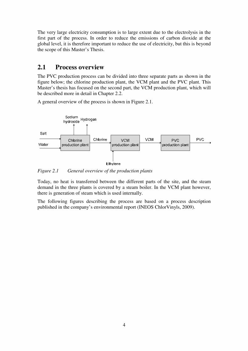
The PVC production process can be divided into three separate parts as shown in the figure below; the chlorine production plant, the VCM plant and the PVC plant. This Master’s thesis has focused on the second part, the VCM production plant, which will be described more in detail in Chapter 2.2.
A general overview of the process is shown in Figure 2.1.
Figure 2.1 General overview of the production plants
Today, no heat is transferred between the different parts of the site, and the steam demand in the three plants is covered by a steam boiler. In the VCM plant however, there is generation of steam which is used internally.
The following figures describing the process are based on a process description published in the company’s environmental report (INEOS ChlorVinyls, 2009).

5
2.1.1 The chlorine plant
Figure 2.2 Present chlorine production
Chemical reaction: 2NaCl + 2H2O → 2NaOH + H2+ Cl2
Today, electrolysis is used to produce chlorine from common salt as seen in Figure 2.2. Hydrogen gas and sodium hydroxide are produced as well. The current production technology uses mercury and needs to be replaced in a few years. The planned chlorine production plant will use membrane technology and will have a larger production capacity than the existing plant.
Since chlorine is currently produced by electrolysis, electricity is the dominating energy source in the chlorine plant. The chlorine production plant consumes about 380 GWh of electricity and 8 GWh of steam annually (INEOS ChlorVinyls, 2008).
The energy demand in the planned chlorine production plant using membrane technology will differ from the current demand. The membrane process uses electrolysis as well, but the anolyte and the catolyte are separated by a cation-exchange membrane, that selectively transmits sodium ions (Schmittinger et al, 2006). The membrane process is more energy efficient. Therefore the electricity demand of the membrane process will be lower than for the current process. However, since the production capacity will be increased the total electricity use will be larger. The NaOH produced using the membrane technology will be more diluted than today’s’ NaOH (Schmittinger et al, 2006). The sodium hydroxide needs to be concentrated before it can be sold, and therefore heat will be needed, resulting in a larger steam demand in the new chlorine production plant.
6
2.1.2 The VCM plant
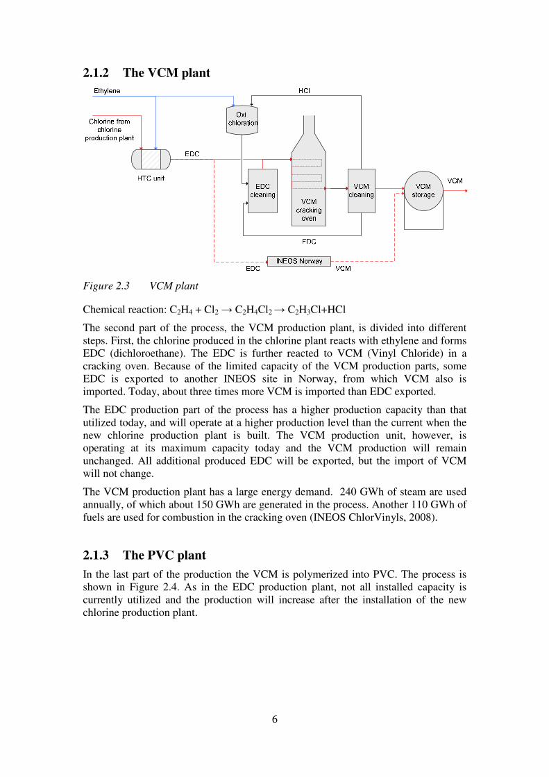
Figure 2.3 VCM plant
Chemical reaction: C2H4 + Cl2 → C2H4Cl2 → C2H3Cl+HCl
The second part of the process, the VCM production plant, is divided into different steps. First, the chlorine produced in the chlorine plant reacts with ethylene and forms EDC (dichloroethane). The EDC is further reacted to VCM (Vinyl Chloride) in a cracking oven. Because of the limited capacity of the VCM production parts, some EDC is exported to another INEOS site in Norway, from which VCM also is imported. Today, about three times more VCM is imported than EDC exported.
The EDC production part of the process has a higher production capacity than that utilized today, and will operate at a higher production level than the current when the new chlorine production plant is built. The VCM production unit, however, is operating at its maximum capacity today and the VCM production will remain unchanged. All additional produced EDC will be exported, but the import of VCM will not change.
The VCM production plant has a large energy demand. 240 GWh of steam are used annually, of which about 150 GWh are generated in the process. Another 110 GWh of fuels are used for combustion in the cracking oven (INEOS ChlorVinyls, 2008).
2.1.3 The PVC plant
In the last part of the production the VCM is polymerized into PVC. The process is shown in Figure 2.4. As in the EDC production plant, not all installed capacity is currently utilized and the production will increase after the installation of the new chlorine production plant.
7
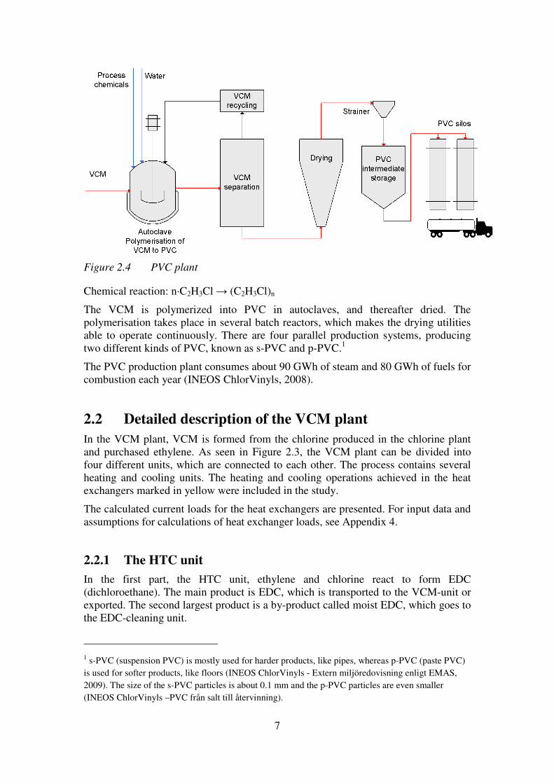
Figure 2.4 PVC plant
Chemical reaction: n·C2H3Cl → (C2H3Cl)n
The VCM is polymerized into PVC in autoclaves, and thereafter dried. The polymerisation takes place in several batch reactors, which makes the drying utilities able to operate continuously. There are four parallel production systems, producing two different kinds of PVC, known as s-PVC and p-PVC.1
The PVC production plant consumes about 90 GWh of steam and 80 GWh of fuels for combustion each year (INEOS ChlorVinyls, 2008).
2.2 Detailed description of the VCM plant
In the VCM plant, VCM is formed from the chlorine produced in the chlorine plant and purchased ethylene. As seen in Figure 2.3, the VCM plant can be divided into four different units, which are connected to each other. The process contains several heating and cooling units. The heating and cooling operations achieved in the heat exchangers marked in yellow were included in the study.
The calculated current loads for the heat exchangers are presented. For input data and assumptions for calculations of heat exchanger loads, see Appendix 4.
2.2.1 The HTC unit
In the first part, the HTC unit, ethylene and chlorine react to form EDC (dichloroethane). The main product is EDC, which is transported to the VCM-unit or exported. The second largest product is a by-product called moist EDC, which goes to the EDC-cleaning unit.
1 s-PVC (suspension PVC) is mostly used for harder products, like pipes, whereas p-PVC (paste PVC) is used for softer products, like floors (INEOS ChlorVinyls - Extern miljöredovisning enligt EMAS, 2009). The size of the s-PVC particles is about 0.1 mm and the p-PVC particles are even smaller (INEOS ChlorVinyls –PVC från salt till återvinning).

8
Figure 2.5 The HTC-unit
The main energy demand is for cooling in the HTC-unit. The only heating needed is in the tricolumn. In the existing process, 8 heat exchangers are in use, although the reboilers and the condenser to the tricolumn are only used part of the time. H164 and H165 are not in use today, but will probably be in use when the production increases. The heat exchanger with the largest duty is the HTC-condenser at the top of the HTC-column.
Table 2.3 Calculated loads of the heat exchangers in the HTC unit, for current
operating conditions
Description: Load [kW]: Utility:
H153 HTC-condenser 9500 Cooling water H154 EDC-condenser 150 Cooling water H155 Remaining gas condenser 5 Propene H158AB Reboiler Tri-column HTC 170 10 bar steam H159 Condenser Tri-column HTC 160 Cooling water H160 Pure EDC-cooler 360 Cooling water H166 Cooler 30 Cooling water
In H155 the process fluid is cooled down to -16°C, and thus refrigerant is required instead of cooling water.

9
2.2.2 The VCM unit
In the VCM unit, the EDC produced in the other parts reacts and forms VCM (Vinyl chloride). VCM is the desired product of the VCM plant. In this unit, hydrochloric acid is formed as well, and is transported to the OXI unit (see chapter 2.2.3). Moist EDC is left as a by-product, and is transported to the EDC-cleaning part.
Figure 2.6 The VCM unit
In the VCM unit, 14 different heat exchangers are studied. The largest cooling demand occurs in the condensers on the cooling column after the cracker. The cracker consumes a lot of fuel but was not included in this study, since it is not possible to replace the fuel with increased heat exchanging. The heat in the flue gases was not included in the main analysis, but is discussed in a later section (Chapter 4.7), where increased energy utilisation from the flue gases was investigated.
10
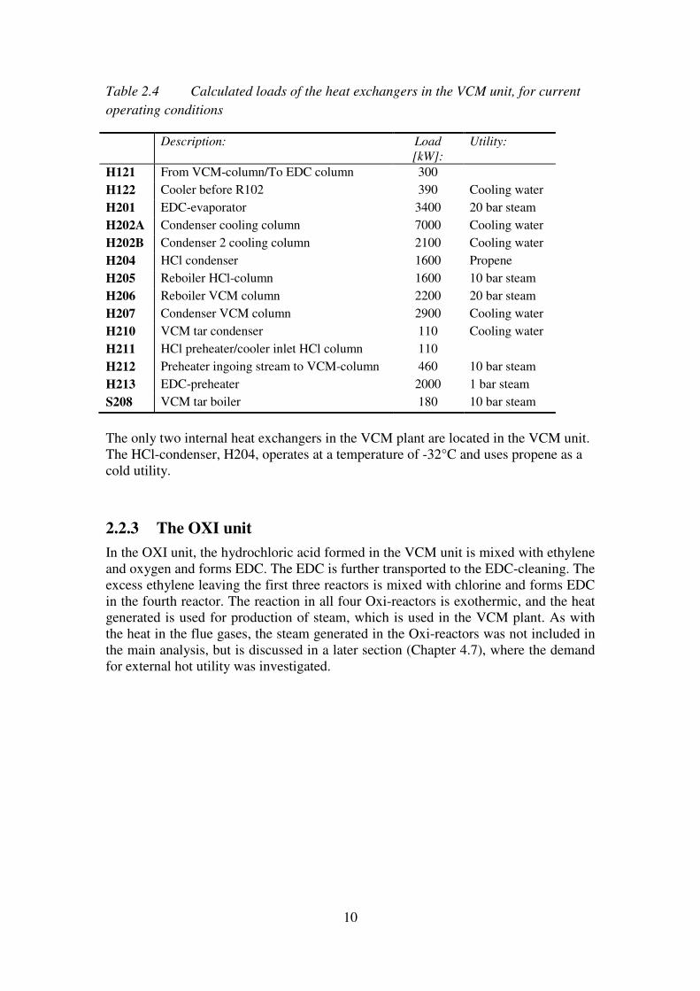
Table 2.4 Calculated loads of the heat exchangers in the VCM unit, for current
operating conditions
Description: Load [kW]:
Utility:
H121 From VCM-column/To EDC column 300 H122 Cooler before R102 390 Cooling water H201 EDC-evaporator 3400 20 bar steam H202A Condenser cooling column 7000 Cooling water H202B Condenser 2 cooling column 2100 Cooling water H204 HCl condenser 1600 Propene H205 Reboiler HCl-column 1600 10 bar steam H206 Reboiler VCM column 2200 20 bar steam H207 Condenser VCM column 2900 Cooling water H210 VCM tar condenser 110 Cooling water H211 HCl preheater/cooler inlet HCl column 110 H212 Preheater ingoing stream to VCM-column 460 10 bar steam H213 EDC-preheater 2000 1 bar steam S208 VCM tar boiler 180 10 bar steam
The only two internal heat exchangers in the VCM plant are located in the VCM unit. The HCl-condenser, H204, operates at a temperature of -32°C and uses propene as a cold utility.
2.2.3 The OXI unit
In the OXI unit, the hydrochloric acid formed in the VCM unit is mixed with ethylene and oxygen and forms EDC. The EDC is further transported to the EDC-cleaning. The excess ethylene leaving the first three reactors is mixed with chlorine and forms EDC in the fourth reactor. The reaction in all four Oxi-reactors is exothermic, and the heat generated is used for production of steam, which is used in the VCM plant. As with the heat in the flue gases, the steam generated in the Oxi-reactors was not included in the main analysis, but is discussed in a later section (Chapter 4.7), where the demand for external hot utility was investigated.

11
Figure 2.7 The OXI unit
In the OXI unit there are 12 heaters or coolers. The unit has a higher demand for cooling than for heating, because of the condensation after the exothermic reactors.
Table 2.5 Calculated loads of the heat exchangers in the OXI unit, for current
operating conditions
Description: Load [kW]:
Utility:
H301 HCl heater 340 10 bar steam H302 Precooler 2600 Cooling water H303AB Condenser after precooler H302 1600 Cooling water H304AB Heater before R304 250 10 bar steam H305 Condenser after R304 380 Cooling water H306 Remainder gas condenser 240 Propene H307 Chlorine evaporator 110 1 bar steam H308 Ethylene preheater 240 10 bar steam H321 Intermediate air cooler 310 Cooling water S210 HCl- evaporator 60 10 bar steam
Since the process fluid in H306 is to be cooled down to -21°C, propene is used.
HCl(g)
from HCl-
column at VCM
635-H308
Ethylene preheater
Steam
10 bar
HCl
(liquid)
Steam
10 bar
Steam
20 bar
635-H301
HCl
heater
625-S210
HCl
evaporator
Air
Cooling
water
635-H321
Intermediate
cooler
Oxygen
Steam
20 bar
produced
635-
R301
Oxi reactor
1
635-
R303
Oxi reactor
3
635-
R302
Oxi reactor
2
Chlorine Steam 1 bar
produced
635-H302
Precooler
635-H303A
Condenser
635-H303B
Condenser
635-H304A
Heat exchanger
635-H304B
Heat
exchanger
635-
R304
Oxi reactor
4
635-H307
Chlorine
evaporator
635-H305
Condenser
635-H306
Remainder gas
condenser
For combustion
Moist EDCTo EDC-
cleaning
Steam
1 bar
Steam 10 bar
Cooling
water
Cooling water
Propene
Ethylene
From HTC
615-H166
Cooling
water
12
2.2.4 The EDC-cleaning unit
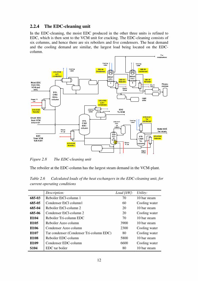
In the EDC-cleaning, the moist EDC produced in the other three units is refined to EDC, which is then sent to the VCM unit for cracking. The EDC-cleaning consists of six columns, and hence there are six reboilers and five condensers. The heat demand and the cooling demand are similar, the largest load being located on the EDC-column.
Figure 2.8 The EDC-cleaning unit
The reboiler at the EDC-column has the largest steam demand in the VCM-plant. Table 2.6 Calculated loads of the heat exchangers in the EDC-cleaning unit, for
current operating conditions
Description: Load [kW]: Utility:
685-03 Reboiler EtCl-column 1 70 10 bar steam 685-05 Condenser EtCl column1 60 Cooling water 685-04 Reboiler EtCl-column 2 20 10 bar steam 685-06 Condenser EtCl-column 2 20 Cooling water H104 Reboiler Tri-column EDC 70 10 bar steam H105 Reboiler Azeo column 3900 10 bar steam H106 Condenser Azeo column 2300 Cooling water H107 Tar condenser (Condenser Tri-column EDC) 80 Cooling water H108 Reboiler EDC-column 5800 10 bar steam H109 Condenser EDC-column 6600 Cooling water S104 EDC tar boiler 80 10 bar steam

13
2.3 Assumptions about the future VCM plant
After construction of the new chlorine plant, the production capacity is assumed to be increased by 100%. This means that the flow into the VCM production plant will be doubled. The EDC production part, the HTC unit, has a higher production capacity than utilized today and the production will have a twofold increase. However, the VCM production is limited, and the VCM unit is operating at its maximum today. The abundance of EDC will be exported to a site in Norway, from which VCM will be imported. Both the production and the import of VCM will remain unchanged, and hence there will be no change in the PVC production plant.
The flow rates into the HTC reactor will be doubled, and consequently the heat and cooling demands for the HTC unit will be doubled. However, the reflux from the HTC-condenser on top of the HTC-column is limited, and cannot exceed 120 m3/h, in order to avoid flooding of the column. This means that some of the cooling demand has to be covered by other coolers. As seen in Figure 2.6, the heat exchangers that first will be taken into use will be the already existing heat exchangers H164 and H165, but there will probably be a need for investment in an additional cooler (Hnew) as well.
Today the tri-column is only used one third of the time. When the production is extended, it is assumed that the tri-column will be used continuously but on a level corresponding to 2/3 of the level today. The production of EDC is assumed to be doubled, and hence the load of the pure EDC-cooler, 615-H160, is also assumed to be doubled. The situation at the top of the HTC-column is more complicated. As mentioned, the reflux is limited, and cannot increase by more than 38%. However, the production of light products is assumed to be doubled, like the production of all other products. This means that a new steady-state is assumed to be reached, with a slightly higher content of volatile compounds in the stream leaving the top of the HTC-column. Since the HTC-condenser is substantially larger than the following coolers, it is possible for the reflux to increase by only 38%, and the mass flow through the following coolers to increase with 100%. The increased flow in the other heat exchangers will barely increase the load of the HTC-condenser, which increases by about 38%. The existing heat exchangers H164 and H165 were modelled using the software “Aspen-designer heat and rating” to approximate their cooling capacity. As earlier mentioned the additional cooling demand is assumed to be covered by a new cooler.
The production capacity of the VCM unit is limited and it is operating at its maximal capacity today, thus the production will remain unchanged. Since the production in the OXI unit is based on the level of hydrochloric acid produced in the VCM unit, it will remain unchanged as well. However, before the fourth reactor, there is a stream

14
coming from the HTC-unit. This one is small compared to the other stream, and the total increase is assumed to be negligible.
The EDC-cleaning unit has incoming streams both from the HTC-unit, the VCM-unit and the OXI-unit. Both the VCM unit and the OXI-unit are assumed to operate at the same level as today. A brief comparison of the different flow rates indicates that if the flow rate from the HTC-unit is increased by a factor of two, and the flow rate from the VCM-unit and the OXI-unit remains constant, the inlet flow rate to the Azeocolumn will increase by approximately 6%. The inlet flow to the EDC-column will increase by 4%. Based on this, the production is assumed to remain unchanged in all units but the HTC unit.
Table 2.7 Summary of assumptions of the future production in the VCM plant
Unit: Description: Future conditions:
VCM No change in production OXI No change in production EDC No change in production HTC H153 HTC-condenser Maximal load before the column floods H154 EDC-condenser Doubled load H155 Remaining gas condenser Doubled load H158AB Reboiler Tri-column HTC 2/3 of today’s load H159 Condenser Tri-column HTC 2/3 of today’s load H160 Pure EDC-cooler Doubled load H166 Cooler Doubled load H164 Cooler Started H165 Cooler Started Hnew Cooler Remaining load

15
3 Methodology
Pinch analysis was used to identify possible energy savings in the VCM plant. Process data was extracted from the process control system and from local measurement points. Simulations in Aspen plus were necessary to approximate flow rates and compositions not measured at the site, and to determine heat exchanger loads. Different measures for increasing the energy efficiency of the plant were investigated. Economic evaluations of the measures as well as an evaluation of reduced carbon dioxide emissions were performed.
3.1 Data extraction
Data was gathered using different sources. At the site, the process operation software “Aspen process explorer” is used, making it possible to access process data. Process data was taken as a mean value for a representative time period. All data and the time period used are listed in Appendix 2. Since the value over a time period can be seen, this is the most trustworthy data. Some data not included in the database was taken from local measurement points, such as pressure indicators, being more uncertain since such data is not measured and recorded continuously. Additional temperatures needed are measured at the pipes in the site, assuming no temperature difference on the inside and the outside of the pipe in the case of steel pipes. In some cases with no possibilities for measurements, data was taken from the site’s process descriptions and equipment design data.
For a plan of the process, including measurement points, please see Appendix 1.
At certain points in the process extractions of the streams are analyzed. Their composition is reported in a program called LabMaster. The points where the compositions are measured are shown in the process plan in Appendix 1. For the case where the composition of the stream is unknown, it is primarily calculated, secondarily simulated in Aspen, and if nothing else is possible the composition is taken from an old Aspen plus simulation of the whole VCM plant, performed in 2001. For process data and assumptions for each heat exchanger, please see Appendix 4.
3.2 Aspen simulations
Aspen plus was used to calculate the heat transferred in the heat exchangers. In some of the cases, where the temperatures in and out of the heater/cooler and the pressure, flow rate and composition were known, the simulations were used only to determine the load of the heat exchangers. However, in some other cases, process simulations had to be used to determine stream data not measured in the process.
The property method used is NRTL (Non-random two-liquid model). The NRTL model can describe vapour-liquid equilibrium for non-ideal solutions, according to the built-in help function in Aspen plus. The NRTL equation uses activity coefficients and has advantages compared to simpler models when handling non ideal-mixtures (Prausnitz, Lichtenthaler, & Azevedo, 1999). One exception is the two coolers after the first three Oxi-reactors in the OXI-part, which is modelled separately. In this case, hydrochloric acid is formed and dissolved into water, for which an electrolyte package had to be activated and the property method ENRTL-RK was used.

16
The composition and the flow rate leaving the Oxi-reactors had to be calculated manually, since there were no measurement points at all. For calculations of the flow rate and composition leaving the Oxi-reactors, please see Appendix 3.
In Appendix 4, there is a summary of the results for the different heat exchangers, and of what input data and assumptions that were used. Because of uncertainties in the data and assumptions, there will be uncertainties in the results. The uncertainties most affecting the results are discussed in Chapter 4.8.
3.3 Pinch analysis
Pinch analysis is a systematic method for identifying opportunities for improving the integration of processes in order to decrease the amount of external heating and cooling needed. This is achieved by increasing the share of heating and cooling that is done by internal heat exchanging. Using pinch analysis, the minimum heating and cooling demand and the maximum potential for heat exchanging can be determined. Thereafter, improvements of the current network are investigated.
A material process flow which must be heated or cooled is defined as a stream. A stream which needs to be heated is defined as a cold stream, and a stream in need of cooling is defined as a hot stream, regardless of their absolute temperature. The heat loads for all hot streams over a temperature range is added, forming the hot composite curve. In the same way a cold composite curve can be formed (Kemp, 2007).
Figure 3.1 Composite curves
The red (uppermost) line in Figure 3.1 represents the hot composite curve, whereas the blue (bottommost) line represents the cold composite curve. For a chosen minimum allowable temperature difference (∆Tmin) in the heat exchangers, the pinch point can be determined. The pinch point is the point where the minimum temperature difference occurs, and limits how much heat that it is possible to recover internally within the process (QHX). Also the minimum heating and cooling demands (QH,min and QC,min) can be calculated from the composite curves. The minimum heating and
QC,min QHX QH,min
100 200 300 400
Q [kW]
T [°C]
100
50
150
200
Pinchtemperature
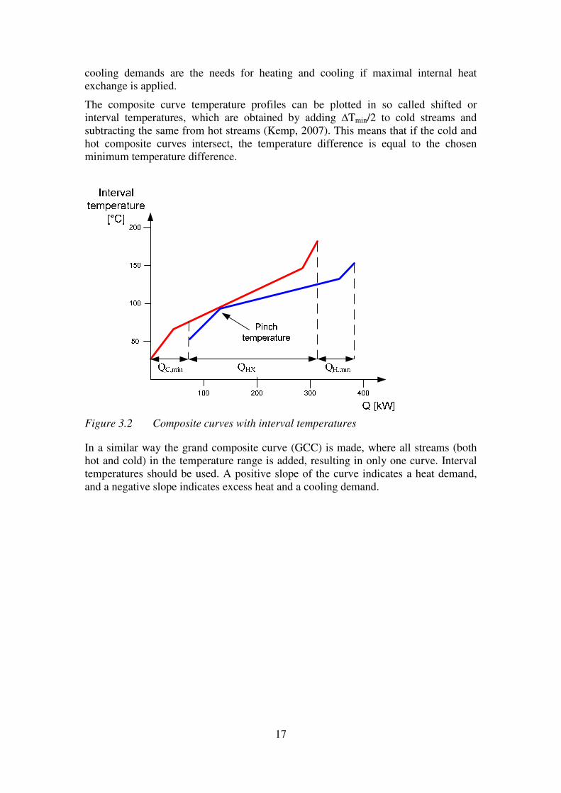
17
cooling demands are the needs for heating and cooling if maximal internal heat exchange is applied.
The composite curve temperature profiles can be plotted in so called shifted or interval temperatures, which are obtained by adding ∆Tmin/2 to cold streams and subtracting the same from hot streams (Kemp, 2007). This means that if the cold and hot composite curves intersect, the temperature difference is equal to the chosen minimum temperature difference.
Figure 3.2 Composite curves with interval temperatures
In a similar way the grand composite curve (GCC) is made, where all streams (both hot and cold) in the temperature range is added, resulting in only one curve. Interval temperatures should be used. A positive slope of the curve indicates a heat demand, and a negative slope indicates excess heat and a cooling demand.
18
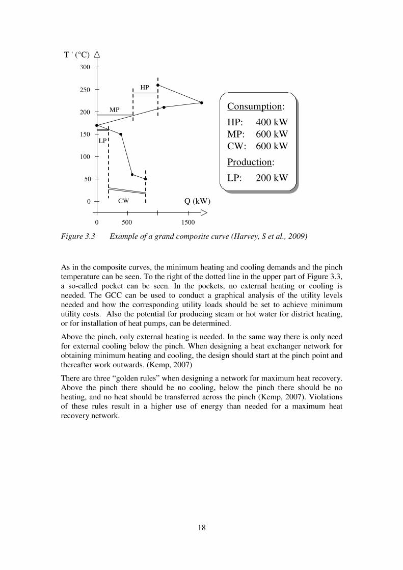
Figure 3.3 Example of a grand composite curve (Harvey, S et al., 2009)
As in the composite curves, the minimum heating and cooling demands and the pinch temperature can be seen. To the right of the dotted line in the upper part of Figure 3.3, a so-called pocket can be seen. In the pockets, no external heating or cooling is needed. The GCC can be used to conduct a graphical analysis of the utility levels needed and how the corresponding utility loads should be set to achieve minimum utility costs. Also the potential for producing steam or hot water for district heating, or for installation of heat pumps, can be determined.
Above the pinch, only external heating is needed. In the same way there is only need for external cooling below the pinch. When designing a heat exchanger network for obtaining minimum heating and cooling, the design should start at the pinch point and thereafter work outwards. (Kemp, 2007)
There are three “golden rules” when designing a network for maximum heat recovery. Above the pinch there should be no cooling, below the pinch there should be no heating, and no heat should be transferred across the pinch (Kemp, 2007). Violations of these rules result in a higher use of energy than needed for a maximum heat recovery network.
300
250
200
150
100
50
T ' (°C)
Q (kW)
500 15000
MP
HP
0
LP
CW
Consumption:
HP: 400 kWMP: 600 kWCW: 600 kW
Production:
LP: 200 kW

19
QH,min
+ Q QH,min
QC,min
QH,min
+ Q
QC,min
+ Q QC,min
+ Q
Q
Q
QPinch temperature
Figure 3.4 Illustration of violations of the three golden rules (Harvey, S et al., 2009)
When studying a site in order to save energy, it is important to identify pinch violations and remove them to improve heat efficiency. Pinch violations can be removed by modifying the temperature range in which the heat exchangers operate, either by installing a new heat exchanger or by changing the order of the existing ones.
A pinch analysis is performed as follows: The first step is to identify which streams that should be included, and thereafter extract stream data. Data extraction is often the most time consuming part of a pinch analysis. The data needed is start and target temperature, and the heat content or demand of the stream. When the data extraction is done, an appropriate value of ∆Tmin is to be chosen. The minimum temperature difference can be set as a global value, or as individual values for each stream. A small minimum temperature difference will allow more heat to be transfered, but will also increase the heat exchanger areas needed. The pinch analysis determines the pinch temperature as well as the minimum process heating and cooling demands. Comparison with the current demands allows the potential for improvements to be determined. Thereafter, the existing network of heaters, coolers and heat exchangers can be examined to identify pinch violations. Pinch violations leads to a higher energy demand than the minumim, as shown in Figure 3.4. When the pinch violations in the existing system are identified, ways to eliminate them should be examined. This could be done by modifying existing heat exchangers, or adding new ones.
For the pinch analysis, the Excel add-in “Pro-pi” was used.
3.4 CO2 emissions evaluation
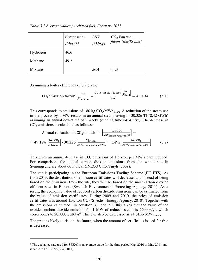
Today, both hydrogen produced at the site and fuel gas bought from a nearby company are used as boiler fuels for steam production. The fuel assumed to decrease in usage when the heat demand decreases is the purchased fuel gas, a mixture of mainly hydrogen and methane. In Table 3.1, the main properties of the fuel are shown. The detailed composition of the gas can be found in Appendix 5.
20
Table 3.1 Average values purchased fuel, February 2011
Composition
[Mol %]
LHV
[MJ/kg]
CO2 Emission factor [ton/TJ fuel]
Hydrogen 46.6
Methane 49.2
Mixture 56.4 44.3
Assuming a boiler efficiency of 0.9 gives:
CO�emission factor � !"#$%&'()* + ,-./01221!" 345 !6 7 &89
:;<='>?@,B + 49.194 (3.1)
This corresponds to emissions of 180 kg CO2/MWhsteam. A reduction of the steam use in the process by 1 MW results in an annual steam saving of 30.326 TJ (8.42 GWh) assuming an annual downtime of 2 weeks (running time 8424 h/yr). The decrease in CO2 emissions is calculated as follows:
Annual reduction in CO�emissions � !" ,-.KL%&'() M'N=O'N·Q6* +
+ 49.194 � !" ,-.#$%&'()* · 30.326 � #$%&'()
KL%&'() M'N=O'N·Q6* + 1492 � !" ,-.KL%&'() M'N=O'N·Q6* (3.2)
This gives an annual decrease in CO2 emissions of 1.5 kton per MW steam reduced. For comparison, the annual carbon dioxide emissions from the whole site in Stenungsund are about 60 kton/yr (INEOS ChlorVinyls, 2009).
The site is participating in the European Emissions Trading Scheme (EU ETS). As from 2013, the distribution of emission certificates will decrease, and instead of being based on the emissions from the site, they will be based on the most carbon dioxide efficient sites in Europe (Swedish Environmental Protecting Agency, 2011). As a result, the economic value of reduced carbon dioxide emissions can be estimated from the value of emission certificates. During 2009 and 2010, the price of emission certificates was around 15€/ ton CO2 (Swedish Energy Agency, 2010). Together with the emissions calculated in equation 3.1 and 3.2, this gives that the value of the avoided carbon dioxide emission for 1 MW of reduced steam is 22000€/yr, which corresponds to 205000 SEK/yr2. This can also be expressed as 24 SEK/ MWhsteam.
The price is likely to rise in the future, when the amount of certificates issued for free is decreased.
2 The exchange rate used for SEK/€ is an average value for the time period May 2010 to May 2011 and is set to 9.17 SEK/€ (E24, 2011).

21
3.5 Economic evaluation
The retrofit proposals were evaluated with respect to economic performance. This was done by using estimated investment costs, and estimated annual utility cost savings and savings because of reduced carbon dioxide emissions to determine payback period for investments in heat recovery equipment.
3.5.1 Investment costs
The investment costs were estimated using the factorial method of cost estimation (Sinnot & Towler, 2009).
First, the area needed for the heat exchanger was calculated from:
� + ����∆�, (3.3)
Where Q is the heat transferred in the heat exchanger, U is the overall heat transfer coefficient (please see Appendix 6), and ∆�, the mean logarithmic temperature, is calculated from:
∆� + VWXYZ,Y[Z\W]Y^_,`ab\cWXYZ,`a\W]Y^_,Y[Zd efgXYZ,Y[Zhg]Y^_,`ai
cgXYZ,`ahg]Y^_,Y[Zdj (3.4)
The heat exchanger is assumed to be aU-tube shell and tube heat exchanger, and the cost of a carbon steel heat exchanger is approximated with (Sinnot & Towler, 2009):
��,�k,�@@l + 24000 m 46 · ���n,� , [$] (3.5)
where ��� is the heat transfer area in the heat exchanger in [m2], and ��,�k,�@@lis the equipment cost for a carbon steel heat exchanger on a US Gulf Coast basis, Jan 2007. (CE index 509.7). In November 2010 the CE index was 556.7 (Chemical engineering, 2011), giving the equipment cost:
��,�k + ��,�k,�@@l · CE index 2010CE index2007 [$] (3.6)
The cost of the heat exchanger, including installation costs, is calculated from (Sinnot & Towler, 2009):
� + ��,�k · fV1 m rsb · r� m cr�t · r� · r� · ru · rv · rdi , (3.7)
where � is the inside battery limits (ISBL) cost, and ��,�k is the cost of the equipment in carbon steel. Together with Eq. 3.6, this gives the inside battery limit cost:
� + ��,�k,�@@l · ,w 1"x/y �@n@,w 1"x/y�@@l · fV1 m rsb · r� m cr�t m r� m r� m ru m rv m rdi
(3.8)
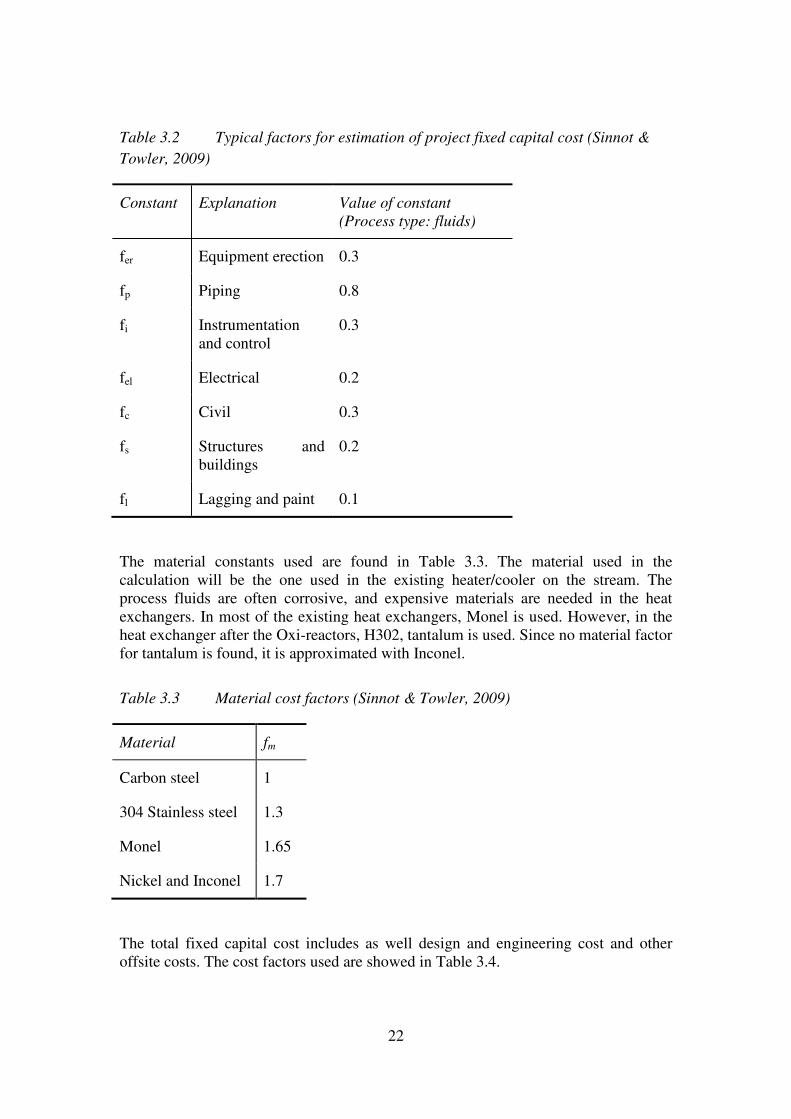
The constants used are found in
Table 3.2 and Table 3.3.
22
Table 3.2 Typical factors for estimation of project fixed capital cost (Sinnot &
Towler, 2009)
Constant Explanation Value of constant (Process type: fluids)
fer Equipment erection 0.3
fp Piping 0.8
fi Instrumentation and control
0.3
fel Electrical 0.2
fc Civil 0.3
fs Structures and buildings
0.2
fl Lagging and paint 0.1
The material constants used are found in Table 3.3. The material used in the calculation will be the one used in the existing heater/cooler on the stream. The process fluids are often corrosive, and expensive materials are needed in the heat exchangers. In most of the existing heat exchangers, Monel is used. However, in the heat exchanger after the Oxi-reactors, H302, tantalum is used. Since no material factor for tantalum is found, it is approximated with Inconel.
Table 3.3 Material cost factors (Sinnot & Towler, 2009)
Material fm
Carbon steel 1
304 Stainless steel 1.3
Monel 1.65
Nickel and Inconel 1.7
The total fixed capital cost includes as well design and engineering cost and other offsite costs. The cost factors used are showed in Table 3.4.
23
Table 3.4 Outside battery limits costs (Sinnot & Towler, 2009)
The total fixed capital cost can be calculated by equation (3.5)(Sinnot & Towler, 2009).
��� + � · c1 m z{d · c1 m |&~ m �d [$] (3.9)
The exchange rate used for USD/SEK is an average value for the time period May 2010 to May 2011 and is set to 6.92 SEK/USD (E24, 2011) .
3.5.2 Annual savings
As in the evaluation of emissions in Chapter 3.4, the decreased use of fuel is assumed to lead to reduced purchase of fuel gas.
The annual savings are calculated from the reduced use of fuel. The price of the fuel is 95 SEK/GJfuel (342SEK/MWhfuel), and the efficiency of the steam boilers is assumed to be 0.9. In the calculations of annual savings, the plant is assumed to have an annual downtime of two weeks.
Fuel savings ��w�Q6 � + �k���� t���u��� �MW� · 8424 � �
Q6* · 3,6 � �$KL�* · B� 7 ���
�;<='>?��Y`^�� (3.10)
This gives reduced fuel costs of 380 SEK/MWhsteam saved, and annual fuel savings of 3.2 MSEK per MW steam saved.
In Chapter 3.4, the savings resulting from decreased carbon dioxide emissions were calculated to 24 SEK/ MWhsteam reduced.
This gives that the total savings are about 400 SEK/MWhsteam saved, and the annual savings are 3.4 MSEK per MW steam reduced in the process.
3.5.3 Payback time
The payback time is calculated as the time to recover the investment cost based on the annual utility cost savings and savings because of reduced carbon dioxide emissions.
Payback time �yr� + �"�/2 0/" 5!2 �K�w�� ""¡4¢ 24�1"£2 �¤���
¥M � (3.10)
No interest rate was considered, since the pay-back period turned out to be short.
Constant Explanation Value of constant (Process type: fluids)
OS Offsite costs 0.3
D&E Design and engineering
0.3
X Contingency 0.1

24

25
4 Results
4.1 System definition and process heating and cooling
requirements
About 50 heat exchangers were included in the study. Most of them are heaters and coolers using heating or cooling utilities, only two are internal stream heat exchangers. Steam at 1, 10, 20 and 28 barg is used for heating, and cooling water and propene are used for cooling. Heat exchanges only used for start-up were not included in the study.
This thesis has focused on the future production, but an analysis of today’s plant was made as well, and is presented in Appendix 8. The current heat demand for the process is 20.9 MW, and the cooling demand is 38.6 MW. The potential for internal heat exchanging is 7.8 MW. All the results shown in this chapter are for the future production level.
The future plant will have a larger cooling demand, because of the increased cooling demand in the HTC unit. The heat demand remains almost unchanged. If no energy efficiency measures are implemented when extending the production, the plant will have a heat demand of 20.8 MW and a cooling demand of 48.9 MW.
The estimated loads of the heat exchangers in the future system are presented in Table 4.1. A more detailed table, with for example condensation temperatures, is found in Appendix 9.
Table 4.1 Process heating and cooling requirements in the future VCM plant,
used for pinch analysis
Unit At: Description Tstart
[C] Ttarget
[C] Q
[kW] Utility 685-03 EDC Reboiler EtCl-column 1 63.8 65 66 10 bar steam
685-04 EDC Condenser EtCl column1 62.9 59.1 60 Cooling water
685-05 EDC Reboiler EtCl-column 2 58.8 59 19 10 bar steam
685-06 EDC Condenser EtCl-column 2 52.9 32.8 19 Cooling water
H104 EDC Reboiler Tri-column EDC 133.6 145.6 74 10 bar steam
H105 EDC Reboiler Azeo column 127.7 128.5 3858 10 bar steam
H106 EDC Condenser Azeo column 85.6 30 2296 Cooling water
H107 EDC Tar condenser (Condenser Tri-column EDC)
87.9 86.5 80 Cooling water
H108 EDC Reboiler EDC-column 111 119.1 5803 10 bar steam
H109 EDC Condenser EDC-column 89.3 35 6634 Cooling water
S104 EDC EDC tar boiler 140 141 78 10 bar steam
H153 HTC HTC-condenser 82.4 74.4 13065 Cooling water
H154 HTC EDC-condenser 73.5 15.8 300 Cooling water
H155 HTC Remaining gas condenser 15.8 -16.5 10 Propene
H166 HTC Cooler 57.5 34 65 Cooling water
H160 HTC Pure EDC-cooler 89.2 26.7 1011 Cooling water
H159 HTC Condenser Tri-column HTC 87.1 13.9 104 Cooling water
26
H158AB HTC Reboiler Tri-column HTC 118 123.5 114 10 bar steam
H165 HTC Cooler R151 115 40 1600 Cooling water
H164 HTC Cooler HTC-column 100 40 1200 Cooling water
Hnew HTC New cooler HTC 100 40 3099 Cooling water
H301 OXI HCl heater 22 179.6 342 10 bar steam
H302 OXI Precooler 217.2 93.9 2618 Cooling water
H303AB OXI Condenser after precooler H302 after R303
93.9 30 1641 Cooling water
H304AB OXI Heater before R304 30.7 137 245 10 bar steam
H305 OXI Condenser after R304 151.5 40 389 Cooling water
H306 OXI Remainder gas condenser 40 -21.5 240 Propene
H307 OXI Chlorine evaporator 3.4 69.6 109 1 bar steam
H308 OXI Ethylene preheater -0.4 119.9 237 10 bar steam
H321 OXI Intermediate air cooler 160 25 307 Cooling water
S210 OXI HCl- evaporator -31.9 41 57,2 10 bar steam
H121-
cold
VCM From VCM-column/To EDC column 41 98 300 Internal heat exchanging
H121-hot VCM From VCM-column/To EDC column 157.7 118 300 Internal heat exchanging
H122 VCM Cooler before R102 118 60 389 Cooling water
H201 VCM EDC-evaporator 193.1 208.61 3442 20 bar steam
H202A VCM Condenser cooling column 132.8 66 7007,5 Cooling water
H202B VCM Condenser 2 cooling column 66 40 2098 Cooling water
H204 VCM HCl condenser -31.7 -32.3 1640 Propene
H205 VCM Reboiler HCl-column 86.5 144.7 1559 10 bar steam
H206 VCM Reboiler VCM column 157.7 158.1 2210 20 bar steam
H207 VCM Condenser VCM column 41.4 17 2880 Cooling water
H210 VCM VCM tar condenser 92.4 52.1 113 Cooling water H211-cold
VCM HCl preheater/cooler in HCl column -32.3 21 110 Internal heat exchanging
H211-hot VCM HCl preheater/cooler in HCl column 40 13 110 Internal heat exchanging
H212 VCM Preheater ingoing stream to VCM-column
81.8 85 457 10 bar steam
H213 VCM EDC-preheater 26.3 118.2 1980 1 bar steam
S208 VCM VCM tar boiler 140 141 178 10 bar steam
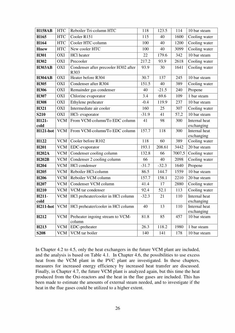
In Chapter 4.2 to 4.5, only the heat exchangers in the future VCM plant are included, and the analysis is based on Table 4.1. In Chapter 4.6, the possibilities to use excess heat from the VCM plant in the PVC plant are investigated. In these chapters, measures for increased energy efficiency by increased heat transfer are discussed. Finally, in Chapter 4.7, the future VCM plant is analyzed again, but this time the heat produced from the Oxi-reactors and the heat in the flue gases are included. This has been made to estimate the amounts of external steam needed, and to investigate if the heat in the flue gases could be utilized to a higher extent.
27
4.2 Pinch analysis of the future VCM plant
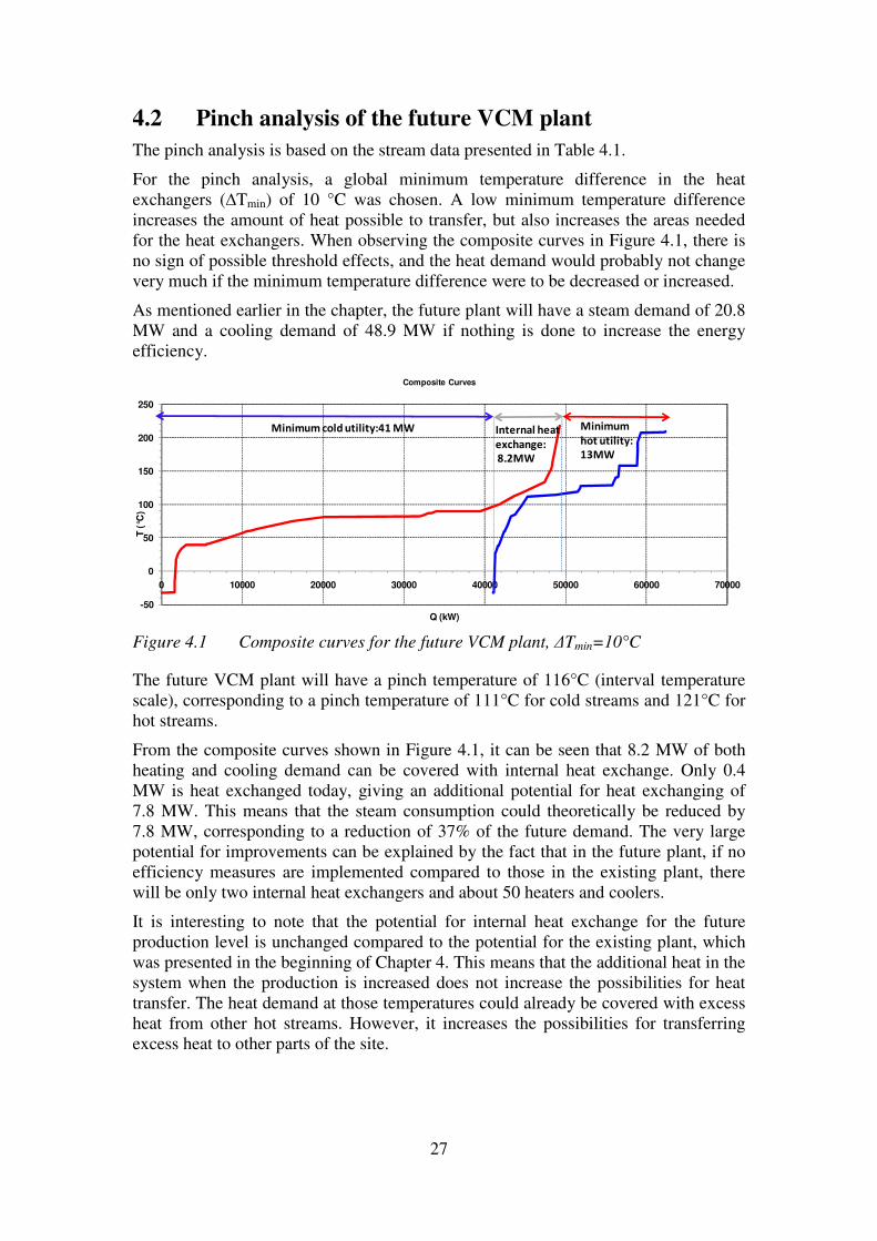
The pinch analysis is based on the stream data presented in Table 4.1.
For the pinch analysis, a global minimum temperature difference in the heat exchangers (∆Tmin) of 10 °C was chosen. A low minimum temperature difference increases the amount of heat possible to transfer, but also increases the areas needed for the heat exchangers. When observing the composite curves in Figure 4.1, there is no sign of possible threshold effects, and the heat demand would probably not change very much if the minimum temperature difference were to be decreased or increased.
As mentioned earlier in the chapter, the future plant will have a steam demand of 20.8 MW and a cooling demand of 48.9 MW if nothing is done to increase the energy efficiency.
Figure 4.1 Composite curves for the future VCM plant, ∆Tmin=10°C
The future VCM plant will have a pinch temperature of 116°C (interval temperature scale), corresponding to a pinch temperature of 111°C for cold streams and 121°C for hot streams.
From the composite curves shown in Figure 4.1, it can be seen that 8.2 MW of both heating and cooling demand can be covered with internal heat exchange. Only 0.4 MW is heat exchanged today, giving an additional potential for heat exchanging of 7.8 MW. This means that the steam consumption could theoretically be reduced by 7.8 MW, corresponding to a reduction of 37% of the future demand. The very large potential for improvements can be explained by the fact that in the future plant, if no efficiency measures are implemented compared to those in the existing plant, there will be only two internal heat exchangers and about 50 heaters and coolers.
It is interesting to note that the potential for internal heat exchange for the future production level is unchanged compared to the potential for the existing plant, which was presented in the beginning of Chapter 4. This means that the additional heat in the system when the production is increased does not increase the possibilities for heat transfer. The heat demand at those temperatures could already be covered with excess heat from other hot streams. However, it increases the possibilities for transferring excess heat to other parts of the site.
-50
0
50
100
150
200
250
0 10000 20000 30000 40000 50000 60000 70000
T (°C
)
Q (kW)
Composite Curves
Minimum cold utility:41 MW Internal heat
exchange:
8.2MW
Minimum
hot utility:
13MW
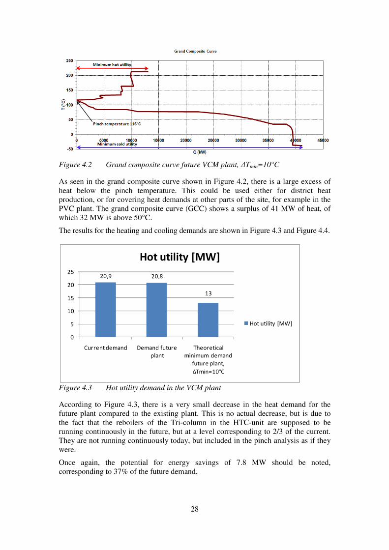
Figure 4.2 Grand composite curve future
As seen in the grand composite curve shown inheat below the pinch temperature. production, or for covering heat demands at other parts of the PVC plant. The grand composite curve (which 32 MW is above 50°C.
The results for the heating and cooling demands are shown
Figure 4.3 Hot utility demand
According to Figure 4.3, there is a very small decrease in the heat demand for the future plant compared to the existing plant. This is no actual decrease, but is due to the fact that the reboilers of the Trirunning continuously in the future, but at a level corresponding to 2/3 of the current. They are not running continuously today, but included in the pinch analysis as if they were.
Once again, the potential for energy savingscorresponding to 37% of the future demand.
20,9
0
5
10
15
20
25
Current demand Demand future
Hot utility [MW]
28
Grand composite curve future VCM plant, ∆Tmin=10°C
As seen in the grand composite curve shown in Figure 4.2, there is a large excess of heat below the pinch temperature. This could be used either for district heat production, or for covering heat demands at other parts of the site, for example in the
grand composite curve (GCC) shows a surplus of 41 MW32 MW is above 50°C.
g and cooling demands are shown in Figure 4.3
Hot utility demand in the VCM plant
, there is a very small decrease in the heat demand for the pared to the existing plant. This is no actual decrease, but is due to
the fact that the reboilers of the Tri-column in the HTC-unit are supposed to be running continuously in the future, but at a level corresponding to 2/3 of the current.
ning continuously today, but included in the pinch analysis as if they
potential for energy savings of 7.8 MW should be noted, corresponding to 37% of the future demand.
20,8
13
Demand future
plant
Theoretical
minimum demand
future plant,
ΔTmin=10°C
Hot utility [MW]
Hot utility [MW]
, there is a large excess of This could be used either for district heat
site, for example in the shows a surplus of 41 MW of heat, of
and Figure 4.4.
, there is a very small decrease in the heat demand for the pared to the existing plant. This is no actual decrease, but is due to
unit are supposed to be running continuously in the future, but at a level corresponding to 2/3 of the current.
ning continuously today, but included in the pinch analysis as if they
of 7.8 MW should be noted,
Hot utility [MW]
29
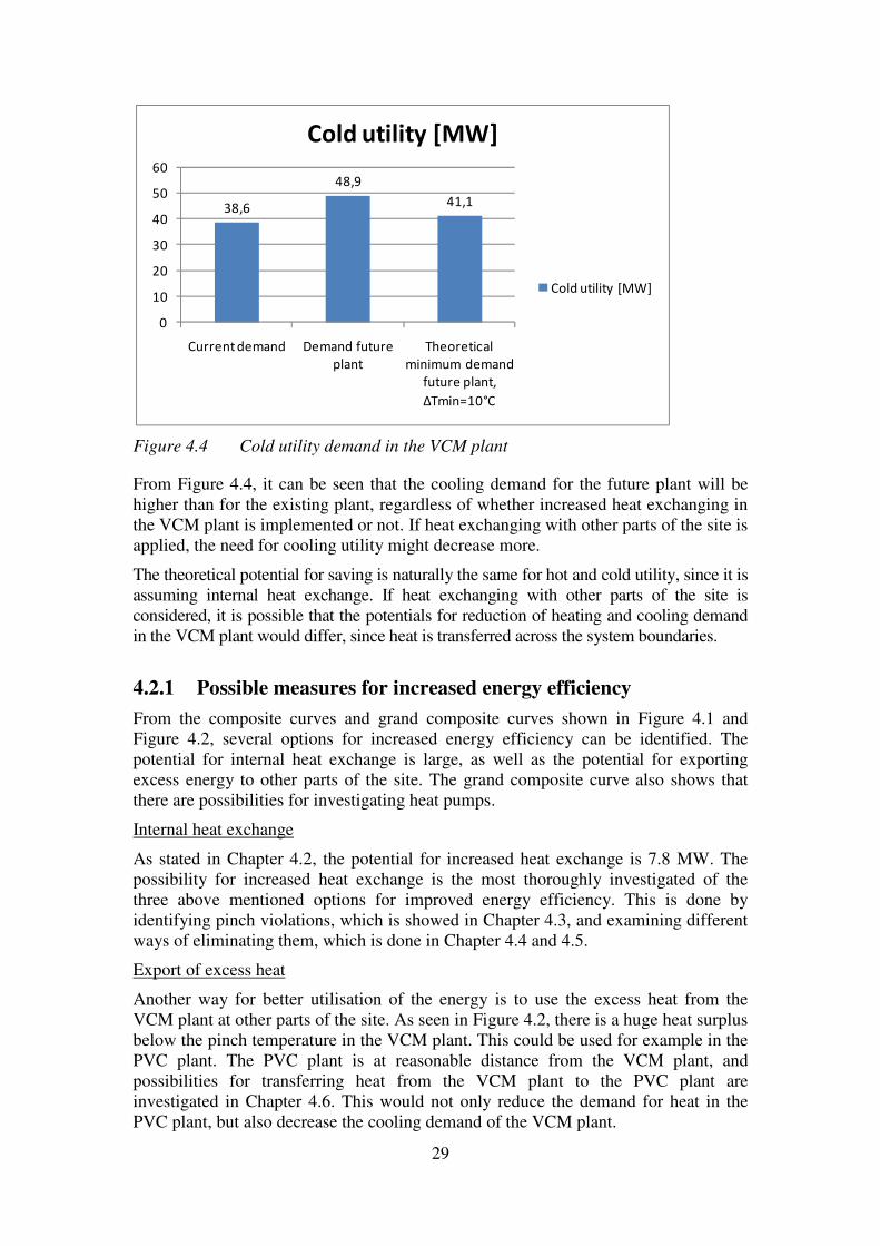
Figure 4.4 Cold utility demand in the VCM plant
From Figure 4.4, it can be seen that the cooling demand for the future plant will be higher than for the existing plant, regardless of whether increased heat exchanging in the VCM plant is implemented or not. If heat exchanging with other parts of the site is applied, the need for cooling utility might decrease more.
The theoretical potential for saving is naturally the same for hot and cold utility, since it is assuming internal heat exchange. If heat exchanging with other parts of the site is considered, it is possible that the potentials for reduction of heating and cooling demand in the VCM plant would differ, since heat is transferred across the system boundaries.
4.2.1 Possible measures for increased energy efficiency
From the composite curves and grand composite curves shown in Figure 4.1 and Figure 4.2, several options for increased energy efficiency can be identified. The potential for internal heat exchange is large, as well as the potential for exporting excess energy to other parts of the site. The grand composite curve also shows that there are possibilities for investigating heat pumps.
Internal heat exchange
As stated in Chapter 4.2, the potential for increased heat exchange is 7.8 MW. The possibility for increased heat exchange is the most thoroughly investigated of the three above mentioned options for improved energy efficiency. This is done by identifying pinch violations, which is showed in Chapter 4.3, and examining different ways of eliminating them, which is done in Chapter 4.4 and 4.5.
Export of excess heat
Another way for better utilisation of the energy is to use the excess heat from the VCM plant at other parts of the site. As seen in Figure 4.2, there is a huge heat surplus below the pinch temperature in the VCM plant. This could be used for example in the PVC plant. The PVC plant is at reasonable distance from the VCM plant, and possibilities for transferring heat from the VCM plant to the PVC plant are investigated in Chapter 4.6. This would not only reduce the demand for heat in the PVC plant, but also decrease the cooling demand of the VCM plant.
38,6
48,9
41,1
0
10
20
30
40
50
60
Current demand Demand future
plant
Theoretical
minimum demand
future plant,
ΔTmin=10°C
Cold utility [MW]
Cold utility [MW]

Heat pump
The heat pump option is the least smaller potential. It is not discussed in the report other than here
When considering a heat pumppinch. This means that the heat pump should use energy from below the pinch, where there is an excess of heat, and deliver it above the pinch, where there is a deheat.
The largest steam consumer in the plant is the reboiler of the EDCcover parts of the demand, it could be possible to install a heat pump, using heat from the condenser. The temperature difference between the reboiler and the condenser is only about 20°C, making investigating a heat pump interesting. be included in some of the proposed retrofits in Chapter cover all the demand of the reboiler, ainvestment in increased heat exchange is made or not. Thplaced across the pinch, causing no pinch violations.
Figure 4.5 Grand composite curve for the future VCM plant, wit
showing a heat pump from the condenser to the reboiler of the EDC
A disadvantage with placing the heat pump at the EDCproblems with fouling.
4.3 Pinch violations
For improving the energy effiexchange, it is important to find and eliminate the pinch violations. shows that there are a totalpinch violations of 7.8 MW. The pinthe pinch violations are located in the HTC part, and it should be mentioned that existing plant and the future
The five biggest pinch violations 83% of the total pinch violations.eliminated, most of the potential for heat saving in the site is achievedheating and the cooling demands could be
30
The heat pump option is the least studied of the mentioned options, because of the It is not discussed in the report other than here.
When considering a heat pump, it is important that the heat pump is placed across the pinch. This means that the heat pump should use energy from below the pinch, where there is an excess of heat, and deliver it above the pinch, where there is a de
sumer in the plant is the reboiler of the EDC-columnthe demand, it could be possible to install a heat pump, using heat from
the condenser. The temperature difference between the reboiler and the condenser is ing investigating a heat pump interesting. The EDC
be included in some of the proposed retrofits in Chapter 4.4. But since they do not cover all the demand of the reboiler, a heat pump could be considered regardless
d heat exchange is made or not. The heat pump would also be placed across the pinch, causing no pinch violations.
Grand composite curve for the future VCM plant, wit
showing a heat pump from the condenser to the reboiler of the EDC-column
A disadvantage with placing the heat pump at the EDC-column is that there could be
Pinch violations in the VCM plant
For improving the energy efficiency of the plant and increase the internal heat exchange, it is important to find and eliminate the pinch violations.
total of 15 pinch violations in the future systempinch violations of 7.8 MW. The pinch violations are shown in Appendix
ons are located in the HTC part, and it should be mentioned that and the future plant will have the same pinch violations.
five biggest pinch violations were investigated in detail, corresponding to about 83% of the total pinch violations. This means that if those five pinch violations are eliminated, most of the potential for heat saving in the site is achieved
ting and the cooling demands could be reduced by 6.5 MW.
studied of the mentioned options, because of the
, it is important that the heat pump is placed across the pinch. This means that the heat pump should use energy from below the pinch, where there is an excess of heat, and deliver it above the pinch, where there is a deficit of
column (H108). To the demand, it could be possible to install a heat pump, using heat from
the condenser. The temperature difference between the reboiler and the condenser is The EDC-column will
. But since they do not heat pump could be considered regardless if an
heat pump would also be
Grand composite curve for the future VCM plant, with ∆Tmin=10°C,
column
column is that there could be
increase the internal heat exchange, it is important to find and eliminate the pinch violations. The analysis
pinch violations in the future system, giving total ppendix 11. None of
ons are located in the HTC part, and it should be mentioned that the
, corresponding to about This means that if those five pinch violations are
eliminated, most of the potential for heat saving in the site is achieved, and both the

31
Table 4.2 The five largest pinch violations in the future VCM plant, ∆Tmin=10°C
At: Description: Cooling above pinch [kW]:
Heating below pinch [kW]:
Heat through pinch [kW]
H302 OXI Precooler after Oxi-reactors
1876
H202A VCM Condenser after cooling column
1680
H205 VCM Reboiler HCl-column
656
H212 VCM Preheater before VCM-column
457
H213 VCM EDC-preheater 1825 Sum selected pinch violations: 3556 2938 Total pinch violations: 3722 3787 277
Most of the pinch violations are located in the VCM and OXI units. In the OXI unit, not less than 8 out of the 10 heaters and coolers are pinch violations. However, only one of them is large enough to be considered further. The HTC unit is the only unit not having any pinch violations, since it almost only needs cooling and the temperatures are below the pinch temperature.
Figure 4.6 Illustration of the five largest pinch violations in the future VCM plant,
∆Tmin=10°C
In Figure 4.6, the pinch violations are illustrated. The pinch temperature is at 116 °C (interval temperature scale).
Ways of eliminating the pinch violations will be investigated in the following chapter.
32
4.4 Proposed measures for increased internal heat
transfer in the future VCM plant
In this chapter, the possibilities for increasing the internal heat exchange are investigated. Here, direct heat transfer is assumed. The possibilities of instead using a hot water system will be discussed in Chapter 4.5.
First, it is very important to note, that the streams are numbered by the heat exchanger that covers their heating or cooling demand today. When referring to them, it is not the actual heat exchanger that is referred to, but the stream passing it. When referring to for example H302, it is not the actual heat exchanger that is meant, but the stream today passing it, with start and target temperatures and a heat load as in the heat exchanger. When discussing heat exchanging between heat exchangers, it is thus between the streams in the current heat exchangers. For all retrofit suggestions, new heat exchangers have been considered. The possibilities of using the existing ones for new purposes are not considered. If the new heat exchangers proposed in the retrofits do not cover the total demand of the stream, the new heat exchanger is assumed to be placed on the upstream side of the existing one.
A maximum energy recovery (MER) network was created, and is shown in Appendix 12. In the MER network, 23 heat exchangers, 22 coolers and 12 heaters are used. An investment in 23 heat exchangers is unrealistic, but the MER network is made to show that it is possible to create a network making the VCM plant to need only 13 MW of steam. For comparison, the future network without any improvements will consist of only 2 heat exchangers.
When examining measures for increased internal heat exchange, focus has been on the five pinch violations selected for further investigation in Chapter 4.3. This does not necessarily mean that the above streams should be heat exchanged with each other. It should be noted that for eliminating the pinch violations in the chosen streams other streams probably have to be included. The streams that are cooled with cooling utility above the pinch should be used for heating other streams above the pinch, and the streams that are today heated with hot utility below the pinch should instead be heated with hot streams from below the pinch.
Above the pinch, there are three major cold streams at suitable temperatures which could be used for utilising the heat in the two chosen hot streams (H302 and H202A). That is the streams in reboiler H105 and reboiler H108, both located in the EDC-cleaning unit, and reboiler H205 which is located in the VCM unit. The reboiler H205 has a heat demand both below and above the pinch, and is one of the chosen pinch violations.
For heating up the chosen streams below the pinch (H205, H212 and H213), the heat below the pinch in the streams H302 and H202 could be used. Also streams from the HTC part could be used, although they are at a slightly lower temperature.

33
Table 4.3 Summary of the streams in the VCM plant chosen for retrofit studies
Heat demand [kW]
Heat surplus [kW]
At: Description: Below pinch:
Above pinch:
Below pinch:
Above pinch:
Pinch violations [kW]
Cold streams
H105 EDC Reboiler Azeo-column
3900
H108 EDC Reboiler EDC-column
5800
H205 VCM Reboiler HCl-column
660 900 660
H212 VCM Preheater before VCM-column 460 460
H213 VCM EDC-preheater 1800 160 1800
Hot streams
H302 OXI Precooler after Oxi-reactors
740 1900 1900
H202 VCM Condenser after cooling column 5300 1700 1700
The locations of the streams are found in the map over the VCM plant in Figure 4.7.
Figure 4.7 A map over the VCM-plant with locations of the discussed heat
exchangers.
Different retrofits have been investigated, of which three will be presented. The different heat exchangers in the retrofit will be economically evaluated, as well as the whole retrofit. The following retrofits are made assuming direct heat transfer. Whether that is reasonable or not will be discussed later in Chapter 4.5.

34
In the following figures, the new heat exchangers are assumed to be placed on the upstream side of the existing heat exchangers, reducing their load. In the calculations, no losses to surroundings are assumed.
As seen in Table 4.2, the steam reduction will be 6.5 MW if all of the chosen pinch violations are eliminated.
4.4.1 Retrofit 1
Retrofit 1 consists of two subsystems, which can be implemented independently of each other. In retrofit 1, large consideration has been taken to the location of the streams.
The streams in system 1 are all located in the VCM unit.
Figure 4.8 Retrofit 1, subsystem 1
The steam savings from system 1 amount to 3.4 MW. Since the location of the streams was of large importance in this retrofit, the stream out from the cooling column is heat exchanged with other streams in the VCM unit. The hot stream has a large amount of heat above the pinch, and since the cold streams are mainly located below the pinch, there will be transfer of heat trough the pinch.
Figure 4.9 Retrofit 1, subsystem 2
The stream leaving the Oxi-reactors is here heat exchanged with reboiler H108. It could as well be heat exchanged with H105, which is located closer, but has a higher temperature and therefore less energy can be transferred. Both streams are above the pinch, and system 2 will not lead to any pinch violations.

35
Together, the subsystems form retrofit 1.
Figure 4.10 Retrofit 1
The reason for the steam savings being only 5.2 MW out of the possible 6.5 MW is the heat transferred through the pinch in subsystem 1. In Figure 4.11, an illustration of the retrofit is shown.
Figure 4.11 Illustration of retrofit 1, with the two subsystems
As seen in Figure 4.11, the streams in the VCM unit are located relatively close to each other. The distance between the stream in the Oxi unit and the EDC-cleaning unit is larger. In this retrofit, the locations of the streams have been of large importance, which resulted in pinch violations. In order to save more energy and to eliminate the pinch violations in retrofit 1, another retrofit is shown, named retrofit 2.
Retrofit 1
H202
H213 H212H205
Q=972kWDown pinch:
656kW
Q=1933kWDown pinch:
600kW
Q=457kW
133 C 126 C 112 C 107 C
87 C
123 C
26 C
116 C
82 C
85 C
H302
H108
217 C 121 C
111 C
113 C
Q=1876kW
Total steam savings:5,2 MW
Out from cooling column
Out from oxi-reactors
Steam savings:1,9 MW
Steam savings:3,4 MW
36
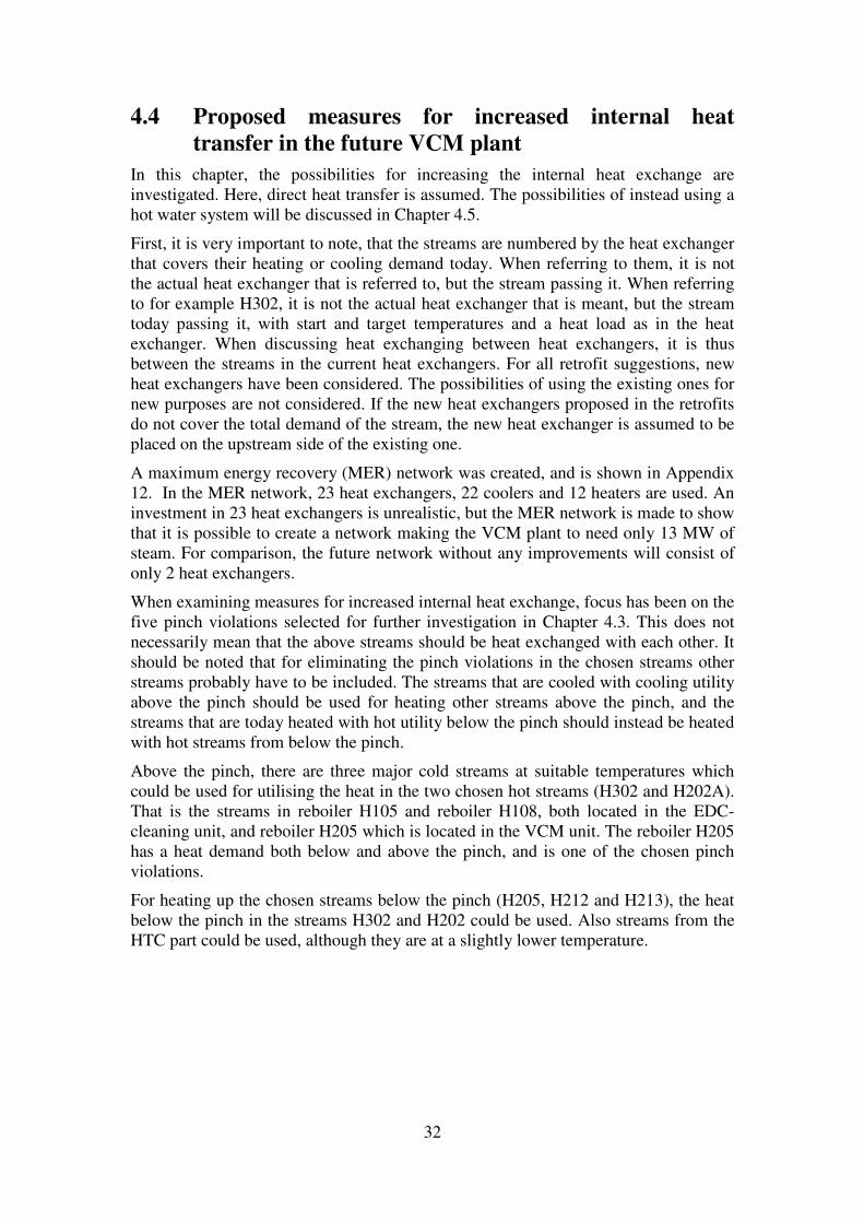
4.4.2 Retrofit 2
Retrofit 2 is an improvement of retrofit 1 regarding steam savings. To avoid the transfer of heat across the pinch that occurs in retrofit 1, the stream out from the cooling could first be heat exchanged with another cold stream.
Figure 4.12 Retrofit 2
In retrofit 2, the heat from the cooling column in the VCM unit is first exchanged with the reboiler H108, before returned to the VCM unit and heat exchanged with the same streams as in retrofit 1. This gives no pinch violations, and hence the steam saving is larger. However, since the stream to H108 is first preheated with the stream from the cooling column before heated with the stream from the Oxi-reactors, the stream from the Oxi-reactors can only almost be cooled down to the pinch temperature, and the steam savings do not reach the maximum possible.
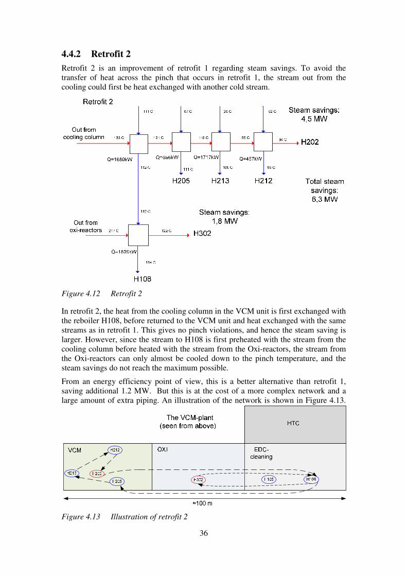
From an energy efficiency point of view, this is a better alternative than retrofit 1, saving additional 1.2 MW. But this is at the cost of a more complex network and a large amount of extra piping. An illustration of the network is shown in Figure 4.13.
Figure 4.13 Illustration of retrofit 2

37
As seen, the hot stream has to be transported to the other end of the site and back. The reasonability of this should be compared with the additional steam savings.
4.4.3 Retrofit 3
None of the two earlier proposed retrofits reached the possible target of saving 6.5 MW when eliminating all pinch violations. Therefore, a third retrofit was investigated.
Figure 4.14 Retrofit 3
Retrofit 3 is based on retrofit 2, with two changes. The stream out from the Oxi-reactors is first heat exchanged with the stream in H105. Thereafter, it is also heating the stream in H205, which is no longer heated with the stream from the cooling column. Retrofit 3 is the only one of the three retrofits that reaches the maximum steam savings of 6.5 MW when eliminating all the pinch violations. This is reached with only five heat exchangers at the expense of a temperature difference slightly less than the specified minimum allowable temperature difference on the cold end of one of the heat exchangers. The temperature difference on the cold end of the heat exchanger H302-H205 is only 9.6°C, and the minimum allowable temperature difference was set to 10°C.
As seen in Figure 4.14, retrofit 3 also consists of two subsystems.
38
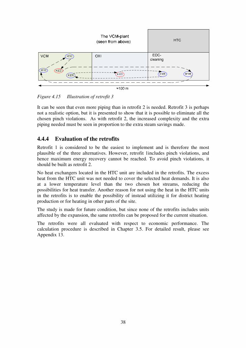
Figure 4.15 Illustration of retrofit 3
It can be seen that even more piping than in retrofit 2 is needed. Retrofit 3 is perhaps not a realistic option, but it is presented to show that it is possible to eliminate all the chosen pinch violations. As with retrofit 2, the increased complexity and the extra piping needed must be seen in proportion to the extra steam savings made.
4.4.4 Evaluation of the retrofits
Retrofit 1 is considered to be the easiest to implement and is therefore the most plausible of the three alternatives. However, retrofit 1includes pinch violations, and hence maximum energy recovery cannot be reached. To avoid pinch violations, it should be built as retrofit 2.
No heat exchangers located in the HTC unit are included in the retrofits. The excess heat from the HTC unit was not needed to cover the selected heat demands. It is also at a lower temperature level than the two chosen hot streams, reducing the possibilities for heat transfer. Another reason for not using the heat in the HTC units in the retrofits is to enable the possibility of instead utilizing it for district heating production or for heating in other parts of the site.
The study is made for future condition, but since none of the retrofits includes units affected by the expansion, the same retrofits can be proposed for the current situation.
The retrofits were all evaluated with respect to economic performance. The calculation procedure is described in Chapter 3.5. For detailed result, please see Appendix 13.

39
Table 4.4 Cost evaluation of the retrofits
Q[kW] Cost of equipment, Nov 2010 [$]
Total fixed capital cost [$]
Total fixed capital cost [MSEK]
Annual savings (utility cost and reduced CO2) [MSEK]
Payback period [years]
Retrofit 1 Subsystem 1 H202-H205 972 580001 280000 1.9 3.3 H202-H213 1933 660001 320000 2.2 6.6 H202-H212 457 490001 240000 1.6 1.6 Sum subsystem 1 5.8 11.5 0.50 Subsystem 2 H302-H108 1876 600002 290000 2.0 6.4
Sum subsystem 2 2.0 6.4 0.31 Sum retrofit 1: 7.8 17.8 0.43
Retrofit 2 H202-H108 1680 870001 420000 2.9 5.7 H202-H205 656 550001 260000 1.8 2.2 H202-H213 1717 660001 320000 2.2 5.9 H202-H212 457 570001 270000 1.9 1.6 H302-H108 1839 600002 290000 2.0 6.3
Sum retrofit 2: 11 21.6 0.50
Retrofit 3 H202-H108 1680 870001 420000 2.9 5.7 H202-H213 1825 660001 320000 2.2 6.2 H202-H212 457 520001 250000 1.7 1.6 H302-H105 973 500002 240000 1.6 3.3 H302-H205 1559 1030002 490000 3.4 5.3
Sum retrofit 3: 12 22.1 0.54
Material used in heat exchanger: 1=Monel, 2=Inconel
From Table 4.4, it can be seen that all of the alternatives are profitable, having a payback time of less than one year. The annual savings is about 20 MSEK. This makes it very interesting from an economic point of view to continue research about the investments.
In the retrofits, one of the most steam saving proposed new heat exchangers is with the stream in H213. In the current process, heater H213 is heated with 1-barg steam. In Chapter 5.1, there is a discussion about how to value the low-pressure steam.
The investment cost might be underestimated. The pipelines that have to be built are probably longer than the standard assumption in the factorial method of cost estimation, especially when heat exchanging between different parts of the plant. The cost of installation could also be higher, due to difficulties of inserting new heat exchangers into the existing units. It is also possible that the material correction factor

40
is too low, since the fluids are corrosive and demand very corrosion-resistant materials. The market price for heat exchanger construction materials has rather high variations, and it is possible that the material price has increased since the correction factors in the model were developed. In reality, there will also be losses of heat, and not as much heat as calculated will be transferred, giving lower savings. Other equipment such as pumps must be installed, increasing the equipment costs and running costs.
On the plus side, there will also be less need for cooling water, which should be accounted for when considering an investment (see Chapter 5.1). The cost for the carbon dioxide emission certificates can be expected to increase in the future, also making the investments more beneficial, even though the profit from the certificates is small compared to the reduced fuel costs. Table 4.5 CO2-evaluation and comparison with MER-network
Reduced heating/cooling demand [MW]
Steam savings compared to maximum recovery network
Annually avoided CO2 emissions [kton]
Retrofit 1 5.2 67% 8.1
Retrofit 2 6.3 82% 9.8
Retrofit 3 6.5 83% 10.1
For comparison, the annual carbon dioxide emissions from the whole site in Stenungsund are currently about 60 kton/yr (INEOS ChlorVinyls, 2009).
In Table 4.5, the energy savings from the retrofits compared to the maximum possible savings from internal heat exchange are shown.
4.5 Hot water system and steam production instead of
direct heat exchange in the future VCM plant
In the previous chapter, retrofits using direct heat exchanging are discussed. However, that is not always possible. The fluids are often corrosive and expensive materials in the pipelines would be needed. Fouling in the equipment is another problem. The matter of safety is important when considering transporting streams across the site and the case of leakage must be considered. There could be leakage in the heat exchanger as well, and if the fluids to be heat exchanged must not be mixed a heat transfer media should be used. Another advantage with a heat transfer media is that the system could be easier to control.
In the case of direct heat transfer between the streams in the plant being unrealistic, a circulating hot water system might be used. When using a hot water system, the minimum temperature difference between the hot and the cold stream must be doubled, since the minimum temperature should occur both between the hot stream and the water and the water and the cold stream. This reduces the potential for heat
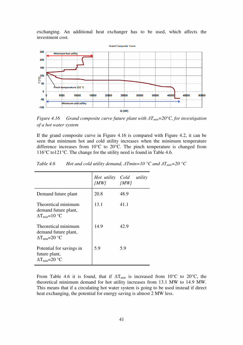
41
exchanging. An additional heat exchanger has to be used, which affects the investment cost.
Figure 4.16 Grand composite curve future plant with ∆Tmin=20°C, for investigation
of a hot water system
If the grand composite curve in Figure 4.16 is compared with Figure 4.2, it can be seen that minimum hot and cold utility increases when the minimum temperature difference increases from 10°C to 20°C. The pinch temperature is changed from 116°C to121°C. The change for the utility need is found in Table 4.6. Table 4.6 Hot and cold utility demand, ∆Tmin=10 °C and ∆Tmin=20 °C
Hot utility [MW]
Cold utility [MW]
Demand future plant 20.8 48.9
Theoretical minimum demand future plant, ∆Tmin=10 °C
13.1 41.1
Theoretical minimum demand future plant, ∆Tmin=20 °C
14.9 42.9
Potential for savings in future plant, ∆Tmin=20 °C
5.9 5.9
From Table 4.6 it is found, that if ∆Tmin is increased from 10°C to 20°C, the theoretical minimum demand for hot utility increases from 13.1 MW to 14.9 MW. This means that if a circulating hot water system is going to be used instead if direct heat exchanging, the potential for energy saving is almost 2 MW less.

42
4.5.1 Proposed retrofits, using hot water systems
The first two retrofit proposals are evaluated for a minimum temperature difference of 20 °C. For a higher minimum temperature approach, not as much heat is transferred through the pinch in retrofit 1. Table 4.7 Reduced heating and cooling demand for retrofit 1 and 2 when having
a minimum temperature difference of 20 °C
Reduced heating/cooling demand [MW]
Retrofit 1 4.5
Retrofit 2 4.7
The reduced utility demand for the different retrofit options is shown in Table 4.7. They should be compared to the total potential for savings of 5.9 MW with a minimum temperature difference of 20°C.
Because of less transfer through the pinch in retrofit 1, retrofit 1 saves almost as much steam as retrofit 2. Retrofit 2 is more complex, with heat from the VCM unit first to the EDC-cleaning to the other side of the plant and then again to the VCM unit. Therefore, it was discarded as a realistic option for a system using circulating hot water for heat transfer.
An investigation of retrofit 1 for a circulating hot water system was conducted. As before, retrofit 1 consists of two subsystems, and two different hot water systems are required. Different flow rates of water in the systems could be used. However, in this preliminary investigation, only one flow rate of water in each system was considered. The flow of water is set to have as large heat recovery as possible. To be able to transfer as much heat as possible to the cold streams, the water flow should be high. However, the capacity rate (FCp) for the water cannot be higher than for the hot stream, if the temperature difference between the streams is to be kept above the minimum allowable temperature difference at all locations within the heat exchanger. Based on this constraint, the flow rate of water was set to equal the capacity rate of the water and the capacity rate of the hot stream.
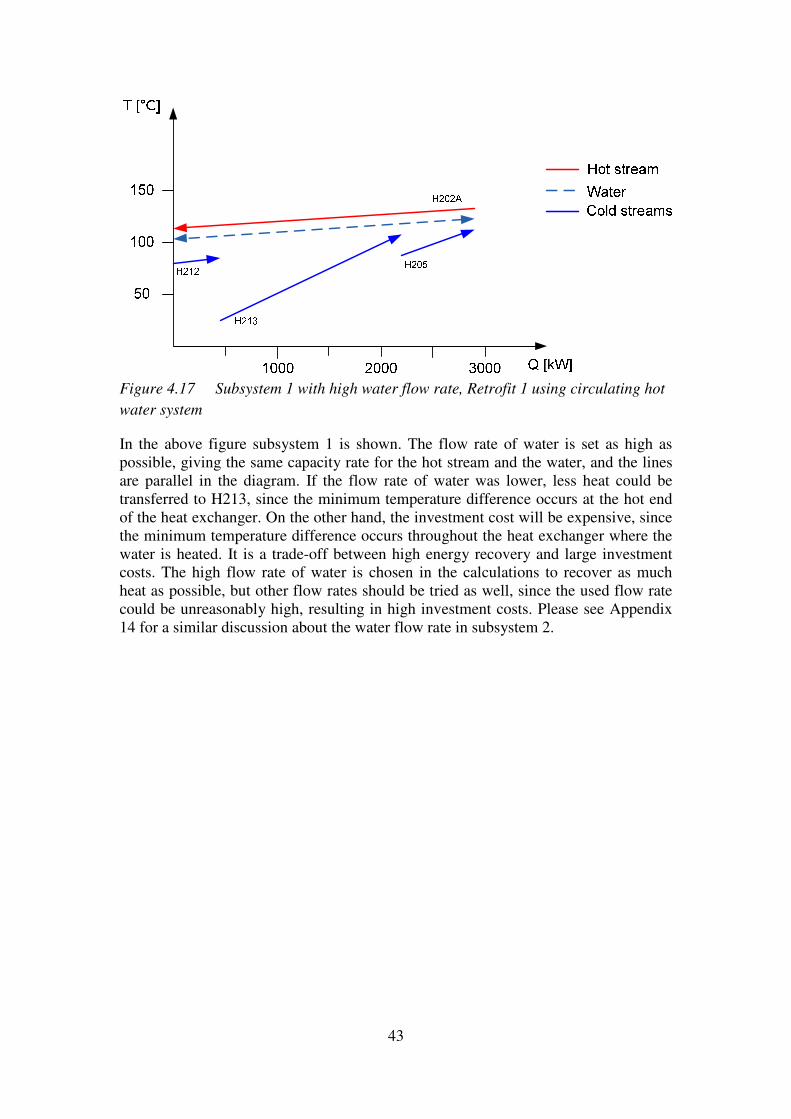
43
Figure 4.17 Subsystem 1 with high water flow rate, Retrofit 1 using circulating hot
water system
In the above figure subsystem 1 is shown. The flow rate of water is set as high as possible, giving the same capacity rate for the hot stream and the water, and the lines are parallel in the diagram. If the flow rate of water was lower, less heat could be transferred to H213, since the minimum temperature difference occurs at the hot end of the heat exchanger. On the other hand, the investment cost will be expensive, since the minimum temperature difference occurs throughout the heat exchanger where the water is heated. It is a trade-off between high energy recovery and large investment costs. The high flow rate of water is chosen in the calculations to recover as much heat as possible, but other flow rates should be tried as well, since the used flow rate could be unreasonably high, resulting in high investment costs. Please see Appendix 14 for a similar discussion about the water flow rate in subsystem 2.

44
Figure 4.18 Retrofit 1 using circulating hot water systems
The steam savings for retrofit 1 with a circulating hot water system is 4.5 MW, compared to 5.2 MW if direct heat transfer is used. In Table 4.8, an economic evaluation of the system shown in Figure 4.18 is made. As seen, the investment cost for the heat exchanger between the stream in H202 and the water is very expensive. This is because of the approach of having the same capacity rate to reach as high energy recovery as possible. This leads to a small temperature difference throughout the heat exchanger, and hence a large heat transfer area is needed. Different flow rates of water should be investigated, and the size of the heat exchangers and the investment cost on the one hand and energy recovery and savings on the other hand should be considered.
Retrofit 1 Hot water systems
H202
H213 H212H205
Q=704kWDown pinch:
208kW
Q=1757kW Q=457kW
123 C
118 C 105 C 102 C
87 C
113 C
26 C
108 C
82 C
85 C
H302 H108217 C 131 C
121 C
179,5 C
Q=1602 kW
102 C
133 C
112 C
FCp water=140 kW/K
Steam savings:2,9 MW
111 C 112 C
121 C
Q=1602 kW
179,5 C
FCp water=27,4 kW/K
Steam savings:1,6 MW
Total steam savings:4,5 MW
Q=2.9MW
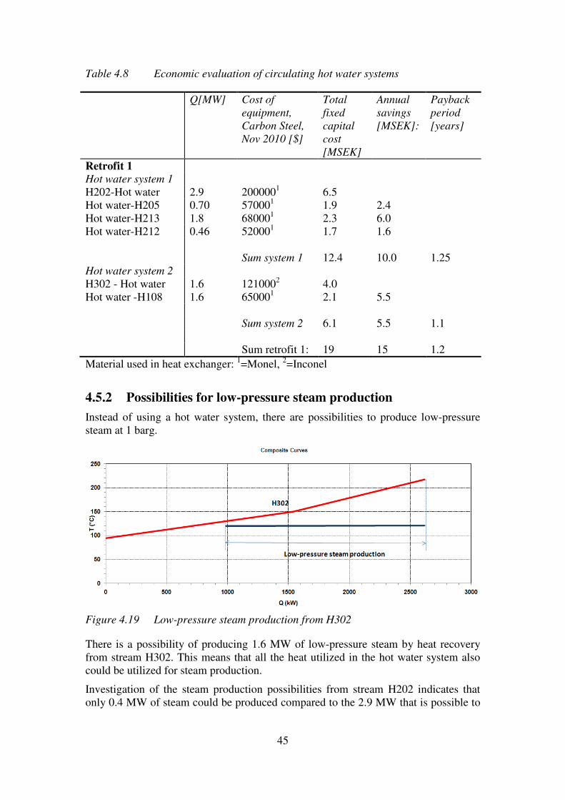
45
Table 4.8 Economic evaluation of circulating hot water systems
Q[MW] Cost of equipment, Carbon Steel, Nov 2010 [$]
Total fixed capital cost [MSEK]
Annual savings [MSEK]:
Payback period [years]
Retrofit 1 Hot water system 1 H202-Hot water 2.9 2000001 6.5 Hot water-H205 0.70 570001 1.9 2.4 Hot water-H213 1.8 680001 2.3 6.0 Hot water-H212 0.46 520001 1.7 1.6 Sum system 1 12.4 10.0 1.25 Hot water system 2 H302 - Hot water 1.6 1210002 4.0 Hot water -H108 1.6 650001 2.1 5.5
Sum system 2 6.1 5.5 1.1 Sum retrofit 1: 19 15 1.2
Material used in heat exchanger: 1=Monel, 2=Inconel
4.5.2 Possibilities for low-pressure steam production
Instead of using a hot water system, there are possibilities to produce low-pressure steam at 1 barg.
Figure 4.19 Low-pressure steam production from H302
There is a possibility of producing 1.6 MW of low-pressure steam by heat recovery from stream H302. This means that all the heat utilized in the hot water system also could be utilized for steam production.
Investigation of the steam production possibilities from stream H202 indicates that only 0.4 MW of steam could be produced compared to the 2.9 MW that is possible to
46
utilize in a circulating hot water system. The results show that from H302 there could be steam production, but from H202 a hot water system has a much higher potential.
4.6 Use of excess heat from the VCM plant in the PVC
plant
In the previous chapters, it was found that there is a large surplus of heat in the VCM plant below the pinch temperature. Options for using this heat in the PVC plant were also investigated.
In the PVC plant, heat can be used both for preheating inlet air for combustion in the drying units, and for heating of low temperature streams. A very rough approximation of the possible heat sinks was conducted, based on an energy mapping of the PVC process (INEOS ChlorVinyls, 2008). In the approximation, it was assumed that the heating fluid has a temperature of 100°C. Assuming a ∆Tmin of 10°C implies that it is possible to heat the cold stream up to 90°C. For calculations, please see Appendix 16.
In the following preliminary assessment, the same price is assumed for saved steam and saved fuel gas. Table 4.9 Approximated heat demand in the PVC plant that could be covered
with 100°C water, ∆Tmin=10°C
Load that can be covered: [MW]
Annual steam/fuel savings: [GJ/yr]
Annual savings, assuming steam price from Chapter 3.5.2 [MSEK/yr]
Preheating of inlet air for drying units:
5 MW 150000 17
Heating of streams:
2 MW 60000 7
Total: 7 MW 230000 24
From Table 4.9, it can be seen that there is a demand for roughly 7 MW of a hot fluid of 100°C in the PVC plant.
The potential for producing hot utility at 100°C from the VCM plant can be estimated based on the GCC in Figure 4.20, assuming a return temperature of the heating fluid to the VCM plant of 50°C.

Figure 4.20 Grand composite curve future
production
The grand composite curve for the future VCM plant of more than 10 MW between 50°C and 100°C. Mthe HTC unit. The condenser at the top of the coolH164, H165 and the new cooler haveIn Figure 4.21, the hot composite curves for thewith the possibilities for pro
Figure 4.21 Composite curve
possibilities for hot water production
It can be seen that the potential for heating water up to 90heating up to 100°C (4.5 Mlowered, the possibilities for transferring more heat arethe composite curves, the heat from the condensation in H153 is barely utilised. possible to heat almost the same amount without using good, since it is a top condenser
47
Grand composite curve future plant, with potential for hot water
The grand composite curve for the future plant shows that there is a heat surplus in the of more than 10 MW between 50°C and 100°C. Much of this is located in
The condenser at the top of the cooling column, and the three coolers H165 and the new cooler have a combined total heat surplus of almost 19 MW.
hot composite curves for these four coolers are shown, together with the possibilities for producing hot water.
Composite curves for H153, H164, H165 and Hnew and the
possibilities for hot water production
It can be seen that the potential for heating water up to 90°C is much larg(4.5 MW compared to 1.6 MW). If the inlet temperature is
possibilities for transferring more heat are of course increased. As seen in , the heat from the condensation in H153 is barely utilised.
possible to heat almost the same amount without using stream H153, which would be it is a top condenser that is hard to access.
h potential for hot water
shows that there is a heat surplus in the of this is located in
ing column, and the three coolers heat surplus of almost 19 MW.
se four coolers are shown, together
H153, H164, H165 and Hnew and the
C is much larger than for the inlet temperature is
of course increased. As seen in , the heat from the condensation in H153 is barely utilised. It is
H153, which would be
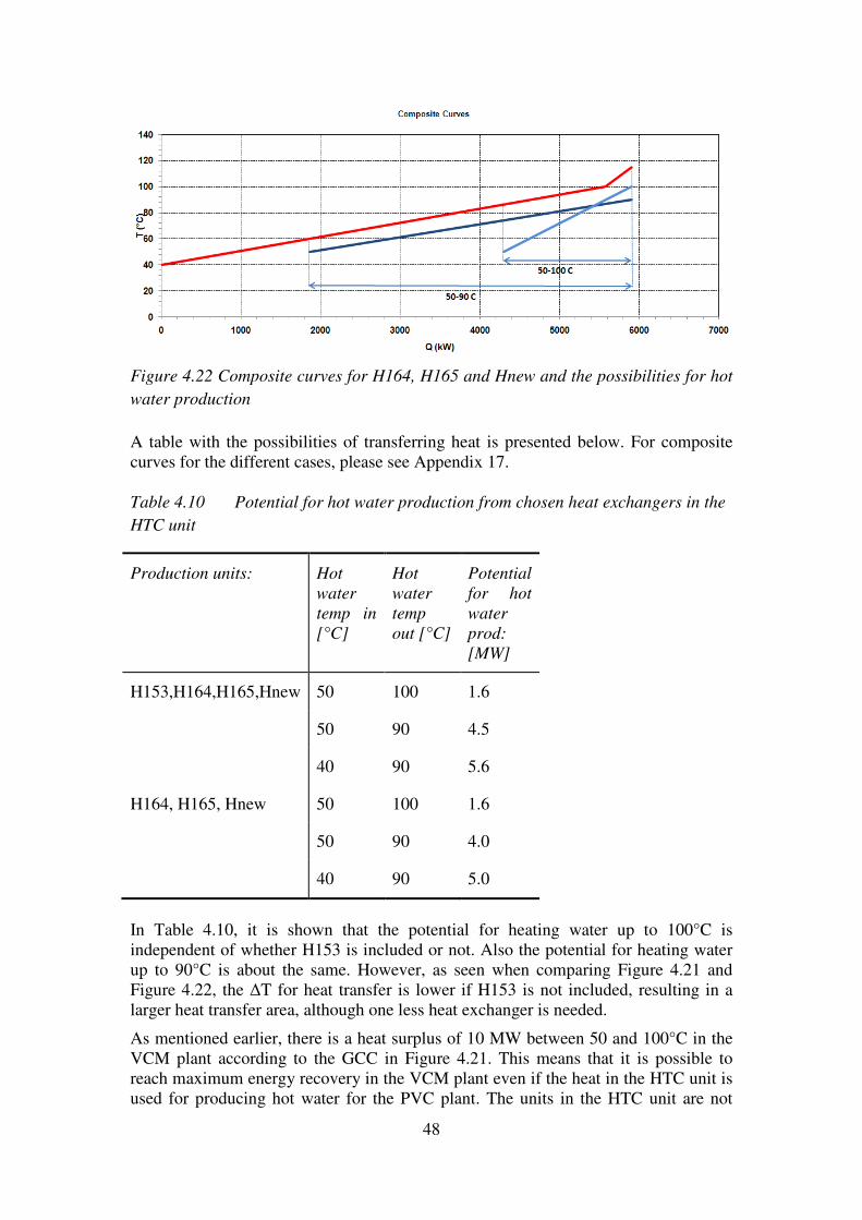
48
Figure 4.22 Composite curves for H164, H165 and Hnew and the possibilities for hot
water production
A table with the possibilities of transferring heat is presented below. For composite curves for the different cases, please see Appendix 17. Table 4.10 Potential for hot water production from chosen heat exchangers in the
HTC unit
Production units: Hot water temp in [°C]
Hot water temp out [°C]
Potential for hot water prod: [MW]
H153,H164,H165,Hnew 50 100 1.6
50 90 4.5
40 90 5.6
H164, H165, Hnew 50 100 1.6
50 90 4.0
40 90 5.0
In Table 4.10, it is shown that the potential for heating water up to 100°C is independent of whether H153 is included or not. Also the potential for heating water up to 90°C is about the same. However, as seen when comparing Figure 4.21 and Figure 4.22, the ∆T for heat transfer is lower if H153 is not included, resulting in a larger heat transfer area, although one less heat exchanger is needed.
As mentioned earlier, there is a heat surplus of 10 MW between 50 and 100°C in the VCM plant according to the GCC in Figure 4.21. This means that it is possible to reach maximum energy recovery in the VCM plant even if the heat in the HTC unit is used for producing hot water for the PVC plant. The units in the HTC unit are not
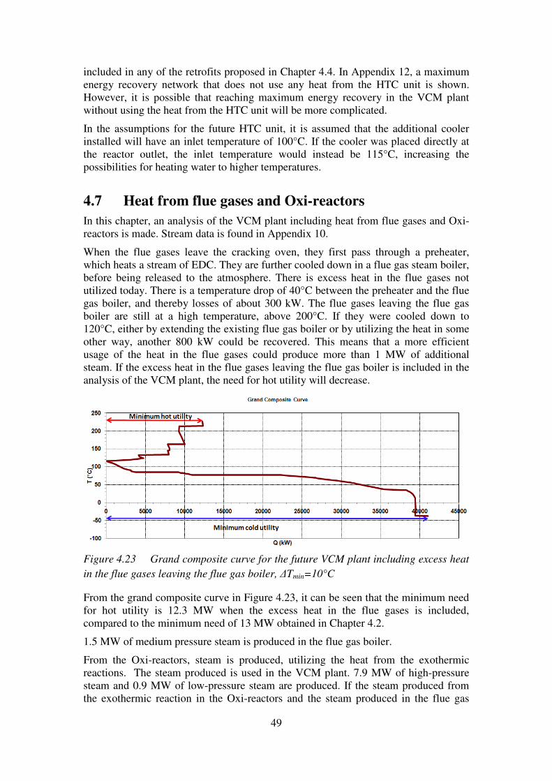
49
included in any of the retrofits proposed in Chapter 4.4. In Appendix 12, a maximum energy recovery network that does not use any heat from the HTC unit is shown. However, it is possible that reaching maximum energy recovery in the VCM plant without using the heat from the HTC unit will be more complicated.
In the assumptions for the future HTC unit, it is assumed that the additional cooler installed will have an inlet temperature of 100°C. If the cooler was placed directly at the reactor outlet, the inlet temperature would instead be 115°C, increasing the possibilities for heating water to higher temperatures.
4.7 Heat from flue gases and Oxi-reactors
In this chapter, an analysis of the VCM plant including heat from flue gases and Oxi-reactors is made. Stream data is found in Appendix 10.
When the flue gases leave the cracking oven, they first pass through a preheater, which heats a stream of EDC. They are further cooled down in a flue gas steam boiler, before being released to the atmosphere. There is excess heat in the flue gases not utilized today. There is a temperature drop of 40°C between the preheater and the flue gas boiler, and thereby losses of about 300 kW. The flue gases leaving the flue gas boiler are still at a high temperature, above 200°C. If they were cooled down to 120°C, either by extending the existing flue gas boiler or by utilizing the heat in some other way, another 800 kW could be recovered. This means that a more efficient usage of the heat in the flue gases could produce more than 1 MW of additional steam. If the excess heat in the flue gases leaving the flue gas boiler is included in the analysis of the VCM plant, the need for hot utility will decrease.
Figure 4.23 Grand composite curve for the future VCM plant including excess heat
in the flue gases leaving the flue gas boiler, ∆Tmin=10°C
From the grand composite curve in Figure 4.23, it can be seen that the minimum need for hot utility is 12.3 MW when the excess heat in the flue gases is included, compared to the minimum need of 13 MW obtained in Chapter 4.2.
1.5 MW of medium pressure steam is produced in the flue gas boiler.
From the Oxi-reactors, steam is produced, utilizing the heat from the exothermic reactions. The steam produced is used in the VCM plant. 7.9 MW of high-pressure steam and 0.9 MW of low-pressure steam are produced. If the steam produced from the exothermic reaction in the Oxi-reactors and the steam produced in the flue gas
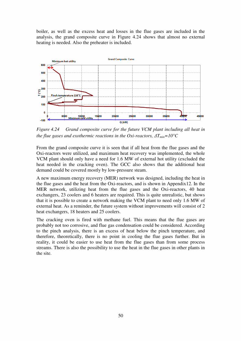
boiler, as well as the excess heatanalysis, the grand composite curve in heating is needed. Also the preh
Figure 4.24 Grand composite curve
the flue gases and exothermic reactions in the
From the grand composite curve it is seen that iOxi-reactors were utilized, and maximum heat recovery was implemented, the whole VCM plant should only have a need for 1.6 MW of external hot utility (excludheat needed in the cracking oven). The GCC also shows that the additional heat demand could be covered
A new maximum energy recovery (MER) network was the flue gases and the heat from thMER network, utilizing heat from the flue gases and the Oxiexchangers, 23 coolers and 6 heatersthat it is possible to create a networkexternal heat. As a reminder, the future system without improvements will consist of 2 heat exchangers, 18 heaters and 25 coolers.
The cracking oven is fired withprobably not too corrosiveto the pinch analysis, there is an excess of heat below the pinch temperature, and therefore, theoretically, there is no point in cooling the flue gases further. But in reality, it could be easier to use heat from the flue gases than from some process streams. There is also the possibility to use the heat in the flue gases in other plants in the site.
50
boiler, as well as the excess heat and losses in the flue gases are included in the analysis, the grand composite curve in Figure 4.24 shows that almost no e
Also the preheater is included.
Grand composite curve for the future VCM plant including
flue gases and exothermic reactions in the Oxi-reactors, ∆Tmin=10°C
From the grand composite curve it is seen that if all heat from the flue gases and the ed, and maximum heat recovery was implemented, the whole
VCM plant should only have a need for 1.6 MW of external hot utility (excludheat needed in the cracking oven). The GCC also shows that the additional heat
mostly by low-pressure steam.
maximum energy recovery (MER) network was designed, including the heat in the flue gases and the heat from the Oxi-reactors, and is shown in Appendix
utilizing heat from the flue gases and the Oxi-reactors,3 coolers and 6 heaters are required. This is quite unrealistic, but shows
that it is possible to create a network making the VCM plant to need only 1.6 MW of As a reminder, the future system without improvements will consist of 2
heat exchangers, 18 heaters and 25 coolers.
fired with methane fuel. This means that the flue gasescorrosive, and flue gas condensation could be considered.
to the pinch analysis, there is an excess of heat below the pinch temperature, and therefore, theoretically, there is no point in cooling the flue gases further. But in reality, it could be easier to use heat from the flue gases than from some process streams. There is also the possibility to use the heat in the flue gases in other plants in
in the flue gases are included in the shows that almost no external
plant including all heat in
0°C
at from the flue gases and the ed, and maximum heat recovery was implemented, the whole
VCM plant should only have a need for 1.6 MW of external hot utility (excluded the heat needed in the cracking oven). The GCC also shows that the additional heat
, including the heat in ppendix12. In the reactors, 40 heat
quite unrealistic, but shows making the VCM plant to need only 1.6 MW of
As a reminder, the future system without improvements will consist of 2
This means that the flue gases are could be considered. According
to the pinch analysis, there is an excess of heat below the pinch temperature, and therefore, theoretically, there is no point in cooling the flue gases further. But in reality, it could be easier to use heat from the flue gases than from some process streams. There is also the possibility to use the heat in the flue gases in other plants in

51
4.8 Uncertainties about the results
There are many uncertainties about the results, due to lack of measurement points and lack of detailed validation of the simulation model. In this section of the report, the uncertainties that are mostly likely to influence the results are discussed. As mentioned earlier, a summary of assumptions for all the different streams is found in Appendix 4.
H205
The temperature out from H205, the reboiler at the HCl-column, is unknown. Also the composition is unknown. The composition is set to consist of only two substances, and the relation between them is set to obtain saturated liquid in to the reboiler. The most uncertain parameter is the temperature out. In the simulations, it is assumed that the vapour fraction of the stream leaving the reboiler is equal to 1.0, resulting in a quite high temperature difference between the inlet and outlet temperature for this mixture. This is probably not true. The vapour fraction could be lower, and the vapour could entrain non-evaporated liquid. The only thing that is known is that the outlet temperature is somewhere between the inlet temperature in and the temperature used. A temperature out of the reboiler of 120 C was tried. When performing a pinch analysis, it does not affect the pinch temperature. However, it affects the potential for internal heat transfer, which is increased by 0.5 MW to 8.7 MW. It also affects the amounts of heat transferred in the proposed retrofits. If the temperature out is lower, the capacity rate for the stream is higher since the heat load is known, and more heat can be transferred to the stream in H205 from the stream in H202. This will lower the possibilities for heating H213, but the total potential for heat exchanging will increase. Stream sheets and composite curves are found in Appendix 18.
H302
The flow rate and composition in H302, the cooler after the Oxi-reactors, are not known. They are calculated from the reaction of the ingoing substances (see Appendix 3). The inlet and outlet temperatures are known, but the condensation level and temperatures are dependent on the property method used in Aspen. The uncertainty about the load of the heat exchanger and of the distribution of the load is large, since it is all based on calculations and Aspen simulations.
H202
In the simulations, the inlet temperature and pressure to H202 are varied to obtain a vapour fraction value of 1.0. This means that the measured inlet temperature is lower than the one used in the analysis. If the temperature is lower, the amount of heat that is possible to transfer will be slightly lower. The assumption about all vapour in the inlet might also be incorrect, overestimating the heat content of the stream. The composition in H202 is unknown, and in the simulations it is taken from an old Aspen simulation. If the actual composition is different, this will affect the condensation energy and the temperature levels for which condensation takes place.

52

53
5 Discussion
In the previous chapter, the main results were presented and discussed. In this chapter, some additional matters are discussed.
5.1 Cooling water and 1-barg steam
Cooling water is usually seen as almost free. But in this case, the cooling demand will increase when the site is retrofitted. As shown, there will be an increase in the VCM plant, but also in the new chlorine plant, which will have a higher cooling demand than the existing one. As a result, the cooling water system needs to be extended, and investment is needed in new coolers to be able to produce the desired amount of cold water. In this case, cooling water is not for free. If the cooling demand can be reduced due to increased internal heat exchange, the expansion needed of the cold water production can be reduced, and the investment cost decreases.
Another utility today estimated as free in the plant is the low-pressure steam. There is an abundance of it, and the low-pressure steam not used for heating will simply be emitted to the surroundings. Therefore, it can be argued that there is no need to replace heat exchangers heated with low pressure steam with heat exchanging. However, there are always ways in which the low-pressure steam could be used. There are possibilities for expanding the low-pressure steam network to include the PVC plant as well, where there is a heat demand. The steam could also be used for increasing the temperature of the proposed hot water production in the HTC unit for use in the PVC plant. Other ways of utilizing the heat include preheating in the boiler house, or heating of buildings at the site. Finally, some of the heat exchangers currently heated with medium pressure steam could instead be heated with low pressure steam.
5.2 Carbon dioxide emissions price
In the economic evaluation, a carbon dioxide price of 15€/ ton was used. This price is likely to increase in the future. However, since the savings because of reduced carbon dioxide emissions only stand for about 5 % of the total savings, this increase will only have a marginal effect on the total savings.
5.3 Other possibilities
As seen in the grand composite curve in Figure 4.20, there is a potential of more than 10 MW for heating water from 50°C to 100°C. This could be used for producing district heating. Today, there is almost no need for additional district heating in Stenungsund. But if the system were connected to the district heating net in Göteborg, there would be a demand (Hackl, R et al., 2011). If the excess heat in the VCM plant could cover both the heat demand in other parts at the site and produce district heating, and which one to be preferred, needs to be examined.
As mentioned several times, there is a heat surplus below the pinch temperature of 116°C. This surplus could be used to cover the heat demands in the PVC plant, but parts of it could also be used for heating the buildings at the site. There are several buildings, and heating them with waste heat from the plant could be investigated.

54
In the proposed retrofits, the heat in the condenser after the cooling column is utilized. If instead it was possible to install a heat exchanger or a steam boiler before the cooling column, after the cracker, heat could be recovered at a higher temperature.
Finally, there is a possibility in several units to use low-pressure steam instead of the medium-pressure steam used today. This would lower the needs of producing steam, since there is an abundance of low-pressure steam today.
5.4 Advantages/disadvantages with hot water production
and steam production instead of direct heat transfer
A hot water system has both advantages and disadvantages compared to direct heat transfer. There is much less risk that the fluids get accidently mixed, and the often corrosive fluid does not have to be transported across the plant in pipes, reducing both the cost for the pipes and the risks for accidents. However, using a hot water system instead of direct heat transfer reduces the amount of heat possible to transfer. This follows as a result of the larger temperature difference needed when hot water first is to be produced from a hot stream, and later to be heating a cold stream. There could be other disadvantages. A condensing stream, for example, stays at the same temperature during the cooling process. This is not the case for a water stream, which could lead to that a very high flow rate of water is needed to transfer all the heat.
There are different possibilities for designing a hot water system. There could be one or more systems, and the heat exchangers could be connected in series or parallel. As mentioned there could also be different flow-rates of water. Those and other possibilities need to be investigated when considering a hot water system.
Another way of utilizing the heat is for production of low-pressure steam. The industry is used to handle steam, and it could probably be used without modifications of the equipment. It also has a high heat content, reducing the amounts needed. But when producing steam, the heat cannot be utilized down to the same temperature levels as if using heat transfer with cold streams. This limits very much how much heat that it is possible to utilize.
5.5 Other comments
In this report, options for using excess heat in the new chlorine plant are not discussed, since very little is known about the planned process. However, there will be a need for steam for evaporating water to concentrate the diluted NaOH produced. It is possible that excess energy from the VCM plant could be used to decrease the steam consumption.
Another comment has to be made regarding the accuracy of the data. The calculated demand for the VCM plant is less than the demand given in the energy mapping earlier made at the company (INEOS ChlorVinyls, 2008). The reasons for this could be that no start-up heaters were included in the analysis, or that the present production level is lower, but it could also be because of poor agreement of the data used.
The same steam price is assumed for all steam levels, independent on pressure, and is based on the energy content in the steam. No limitations of the steam boilers have been considered, or how the efficiency of the boiler will be affected when the production decreases.

55
An interesting possibility in a future scenario could be that if the development of fuel cells is continued, and the market expands, it is possible that there will be an increased demand for hydrogen. In that case, it is possible that it will be more profitable to sell the hydrogen produced instead of using it on-site as boiler fuel.

56
57
6 Conclusions
This thesis investigated the current and future energy demand of the VCM plant, as well as options for increased energy efficiency by internal heat exchange. The study was conducted using pinch analysis methods and tools.
The results show that today’s plant has a heat demand of 21 MW and a cooling demand of 39 MW. When the production is extended in the future, the heat demand will not be affected, but the cooling demand is expected to increase to 49 MW. During the analysis, it was found that there is a large potential for energy savings. Theoretically, the steam use in the future VCM plant could be reduced by 37% by increased internal heat exchange, corresponding to 7.8 MW. Different retrofits have been proposed; of them retrofit 1 is seen as the most reasonable. When considering retrofit 1, it should be remembered that this option does not remove all pinch violations, which means that maximum energy recovery is not reached. To avoid pinch violations, retrofit 2 should be used. Implementing retrofit 1 would lead to a decrease in steam use of 5.2 MW, eliminating 67% of the future pinch violations.
The retrofits were developed assuming direct heat transfer. That may not be possible, due to the composition of the streams used. In that case, implementation of a circulating hot water system may be a possible solution. When using a hot water system, the minimum allowable temperature difference (∆Tmin) between the hot stream and the cold stream must be doubled, in order to respect the minimum allowable temperature difference both when heating and cooling the hot water. This implies that the theoretical demand for steam savings is reduced to 5.9 MW. Implementing retrofit 1 using a hot water system with properties as proposed would in this case lead to a steam reduction of 4.5 MW, corresponding to 76% of the possible steam savings when using hot water systems.
A cost evaluation of the proposed retrofit solutions was also conducted. The investment cost estimations are very rough and should thus be considered with caution. They do however indicate that there is money to be saved with a short payback time. Saving 1 MW of steam leads to annual savings of approximately 3 MSEK, and the total savings could reach 20 MSEK/yr.
It is interesting to conclude that none of the streams proposed for heat exchange is affected by the expansion of the plant. The proposed retrofits are therefore possible to implement whether the production is increased or not. It was also noted that there is a lot of excess heat in the flue gases leaving the cracking oven. If the heat in the flue gases were to be used more efficiently with heat recovery down to 120 °C, another 1 MW of steam could be produced.
The future VCM plant will have a pinch temperature of 116°C (interval temperature scale, ∆Tmin=10°C), corresponding to a pinch temperature of 111°C for cold streams and 121°C for hot streams. This excess heat could be used for different purposes, for example for low temperature needs in the PVC plant. It is interesting to note that maximum energy recovery can be obtained in the VCM plant without the excess heat from the HTC unit. This heat could instead be used for producing hot water, either for use in the PVC plant or for district heating. Approximately 5 MW could be produced in the HTC unit for use in the PVC plant, saving as much steam as the proposed retrofits for the VCM plant.
In conclusion, there is a large potential for increased energy efficiency measures which could reduce both costs and environmental impact.

58
59
7 Future work
The calculated heat loads on some of the heat exchangers needs to be confirmed with measurements. This especially is true for H302, and also for H202. The temperature at the outlet of H205 needs to be measured and compared with the assumed value.
The possibilities for direct heat transfer should be evaluated. If it is considered as not possible, a hot water system should be designed and studied more in detail.
The need for low-temperature heat in the PVC plant should be further investigated, and utilizing excess heat from the VCM plant should be evaluated. But before heat is transferred from the VCM plant to the PVC plant, a similar study should be performed for the PVC plant to see if there is excess heat also in the PVC plant, which should be primarily used. It could also be interesting to perform a study of the whole site to find possibilities for utilizing the excess heat in the VCM plant.
Also, a more detailed economic evaluation should be performed.

60

61
8 References
Chemical engineering. (March 2011). Economic indicators. Chemical engineering vol 118 , s. 64.
E24. (2011). Retrieved May 9, 2011, from E24 Börs: http://bors.e24.com/currencies-stockholm
Hackl, R et al. (2011). Targeting for energy efficiency and improved energy collaboration between different companies using total site analysis (TSA). Energy . doi:10.1016/j.energy.2011.03.023
Hackl, R., Andersson, E. & Harvey, S. (2010). Total site analysis (TSA) Stenungsund. Göteborg: Chalmers University of Technology. (Research project report at the Department of Energy and Environment. Division of Heat and Power technology).
Harvey, S et al. (2009). Industrial energy systems - course compendium. Göteborg: Chalmers University of Technology (Department of Energy and Environment. Division of Heat and Power Technology).
INEOS ChlorVinyls. (2008). Energikartläggning 2008 (Energy mapping 2008. In Swedish). Stenungsund.
INEOS ChlorVinyls. (n.d.). INEOS ChlorVinyls. Retrieved January 17, 2011, from http://www.ineoschlor.com/
INEOS ChlorVinyls. (2009). INEOS ChlorVinyls - Extern miljöredovisning enligt EMAS (INEOS ChlorVinyls- external environmental report accourding to EMAS. In Swedish). Stenungsund: INEOS Sverige AB.
INEOS ChlorVinyls Sweden. (n.d.). Snabbfakta INEOS ChlorVinyls. Retrieved January 17, 2011, from http://ineos.se/183-Snabbfakta.htm
Kemp, I. C. (2007). Pinch Anaysis and Process Integration. Elsevier Ltd.
Prausnitz, J., Lichtenthaler, R., & Azevedo, E. d. (1999). Molecular Thermodynamics of Fluid-Phase Equilibria. Prentice Hall.
Schmittinger et al. (2006). Chlorine. Ullmann's Encyclopedia of Industrial Chemistry
Sinnot, R., & Towler, G. (2009). Chemical engineering design. Elsevier Ltd.
Swedish Energy Agency. (2011). Din uppvärmning (Your heating. In Swedish). Retrieved 06 21, 2011, from http://www.energimyndigheten.se/sv/Hushall/Din-uppvarmning/
Swedish Energy Agency. (2010). Energy in Sweden 2010. Swedish Energy Agency.
Swedish Environmental Protecting Agency. (2011). Handelsperioden 2013-2020 (The trading period 2013-2020. In Swedish). Retrieved May 24, 2011, from Naturvårdsverket:http://www.naturvardsverket.se/sv/Start/Lagar-och-styrning/Ekonomiska-styrmedel/Handel-med-utslappsratter/Handelsperioden-20132020/
Swedish Ministry of the Environment. (2010). Sverige förbjöd användingen av kvicksilver den 1 juni 2009 (Sweden prohibited the use of mercury 1:st of june 2009. In Swedish). Regeringens kemikaliepolitik.
US Energy Information Administration. (2010). International Energy Outlook 2010. Retrieved 01 31, 2011, from http://www.eia.doe.gov/

62
63
9 Appendix
Appendix 1 – Detailed process flowsheets 58
Appendix 2 – Gathered data 62
Appendix 3 – Calculations of composition and flow rate leaving Oxi-reactors 70
Appendix 4 – Assumptions and input data for the heat exchanger calculations 72
Appendix 5 – Properties for the fuel gas 83
Appendix 6 – Heat transfer coefficient 84
Appendix 7 – Current load of heat exchangers 85
Appendix 8 – Pinch analysis of existing VCM plant 87
Appendix 9 – Future load of heat exchangers 89
Appendix 10 – Heat in Oxi-reactors and flue gases 91
Appendix 11 – Pinch violations in the future VCM plant 92
Appendix 12 – MER network future VCM plant 94
Appendix 13 – Economic evaluation of the retrofits 96
Appendix 14 – Hot water calculations 97
Appendix 15 – Economic evaluation hot water system 99
Appendix 16 – Estimation of the low-temperature energy-demand in the PVC plant 100
Appendix 17 – Composite curves using heat from the HTC unit for producing hot water 101
Appendix 18 – H205 with an outlet temperature of 120°C 103

64
Appendix 1 – Detailed process flowsheets

65

66
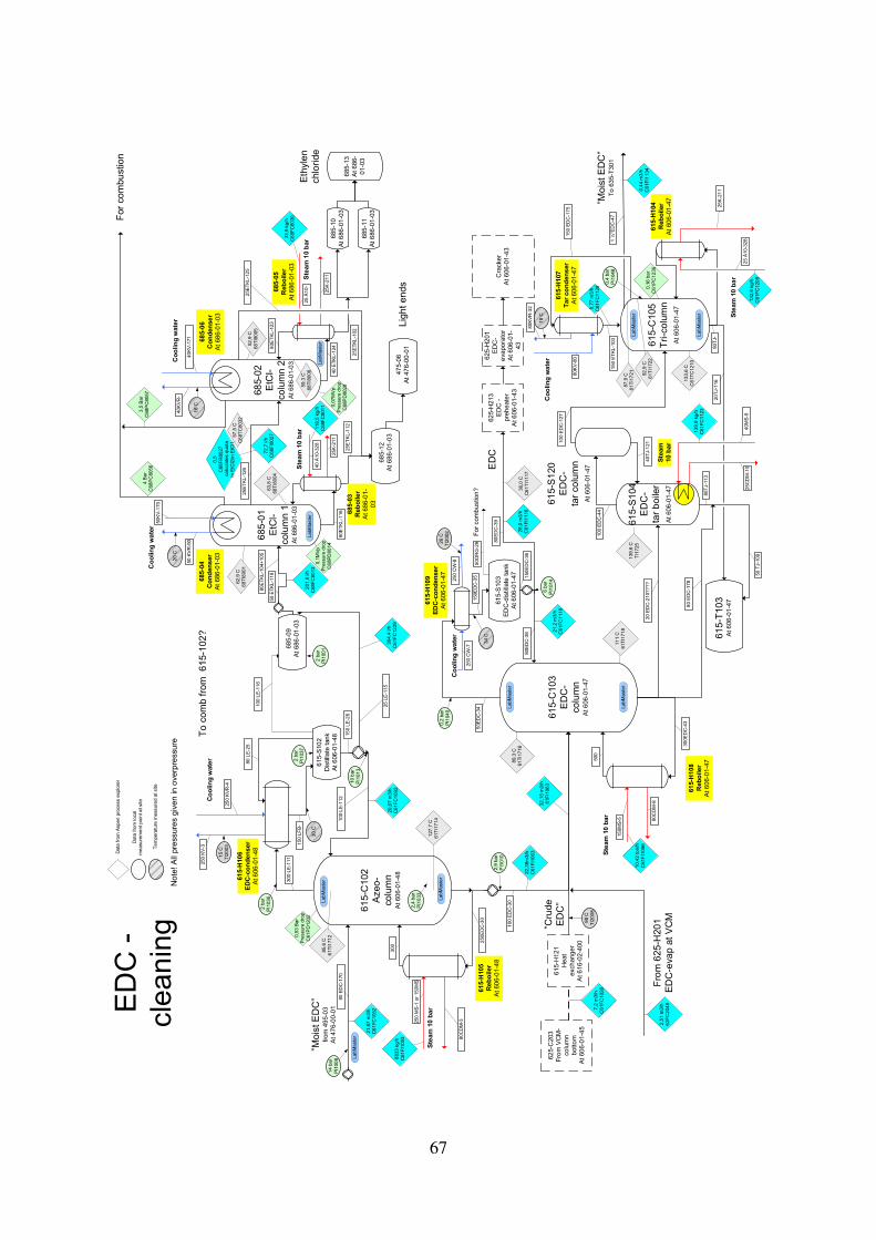
67
0,16 bar
C61P
C1236
25 Å10-328
132,6 kg/h
C61FC1208
25K-211
0,77 m3/h
C61FC1128
150 EDC-175
150 ETKL-103
80KV-80
80KVR-32
32,15 m3/h
61FI1063
2,51 m3/h
62F
C2048
10,42 ton/h
C61FI1096
80CDM-8
150M
S-5
50 ETKL-118
250 CW-8
250 CW-7
150EDC-35
50E
DC-34
22,38m
3/h
C61FI1063
80 EDC-170
21,87 m3/h
C61F
C1052
300
50KV-170
50 KVR-90
40 ETKL-124
150EDC-36
0,07MVp
Pressure drop
C68PD8028
57,5 C
C68T
C8032
3,5 Bar
C68PC8057
0,1M
Vp
Pressure drop
C68P
D8014
80ETKL-116
4 Bar
C68PC8056
150 LE
-26
100 EDC-30
0,53 Bar
Pressure drop
C61PD1202
80 LE-25
150 LFB-
300 LE
-111
100 LE-116
133,6 C
C61TC1210
0,44 m3/h
C61F
I1134
139,9 kg/h
C61FC1123
20 EDC-210????
111 C
61TI1718
80 EDC-178
89,3 C
61TI1716
28,0 m3/h
C61FI1116
80EDC-39
36,0 C
C61T
I1117
21,2 m3/h
C61FC1118
500
7,2 m3/h
C61F
C1028
25E
TKL-102
33,9 kg/h
C68F
C8030
25K-211
25 Å10-
118,5 kg/h
C68FC8011
40 Å10-328
25K-211
25ETKL-112
52,9 C
68TI8005
80E
TKL-123
63,8 C
68TI8004
72,7 l/h
C68FI8027
62,9 C
68T
I8001
0,5
C68FR8027
calculates quota
In EtCl2/in EtCl1
25ETKL-126
80ETKL-104+105
394,4 l/h
C61FC1229
201,9 l/h
C68FC8013
250 KV-3
20,07 m3/h
C61FC1092
6833 kg/h
C61FI1053
250 MS-1 or 150MS
50O
RG-29
100 EDC-44
40M
S-9
300E
DC-43
50 TJ-109
25CDM-10
100 EDC-127
1 ½"EDC-47
20TJ-116
80TJ-
80TJ-113
40TJ-121
80EDC-38
40K
VR-
25E
TKL-125
40KV-171
25 LE-115
250 KVR-4
100 LE-112
250EDC-30
80CDM-3
30 C
615-C102
Azeo-
column
At 606-01-48
615-H105
Reboiler
At 606-01-48
615-H106
EDC-condenser
At 606-01-48
2 bar
PI1037
615-S102
Distillate tank
At 606-01-48
Steam 10 bar
15 C
TI2003
Cooling water
685-09
At 686-01-03
20 C
Cooling water
685-04
Condenser
At 686-01-03
685-01
EtCl-
column 1
At 686-01-03
2 bar
PI1001
Cooling water
685-06
Condenser
At 686-01-03
685-02
EtCl-
column 2
At 686-01-03
16 C
685-10
At 686-01-03
685-11
At 686-01-03
685-13
At 686-
01-03
Ethylen
chloride
For combustion
685-12
At 686-01-03
475-06
At 476-00-01
Light ends
685-03
Reboiler
At 686-01-
03
685-05
Reboiler
At 686-01-03
615-C103
EDC-
column
At 606-01-47
34 C
26 C
TI2002
625-H213
EDC -
preheater
At 606-01-43
625-H201
EDC-
evaporator
At 606-01-
43
Cracker
At 606-01-43
EDC
615-S103
EDC-distillate tank
At 606-01-47
615-H109
EDC-condenser
At 606-01-47
Cooling water
615-H108
Reboiler
At 606-01-47
Steam 10 bar
615-H121
Heat
exchanger
At 616-02-400
625-C203
From VCM-
column
bottom
At 606-01-45
98 C
TI2008
”Crude
EDC”
”Moist EDC”
from 495-03
At 476-00-01
615-S104
EDC-
tar boiler
At 606-01-47
615-C105
Tri-column
At 606-01-47
615-S120
EDC-
tar column
At 606-01-47
615-H104
Reboiler
At 606-01-47
615-H107
Tar condenser
At 606-01-47
Steam
10 bar
Cooling water
615-T103
At 606-01-47
Steam 10 bar
18 C
”Moist EDC”
To 635-T301
For combustion?
To comb from 615-102?
EDC -
cleaning
85,6 C
61T
I1712
127,7 C
61TI1714
Steam 10 bar
59,3 C
68TI8008
Steam 10 bar
87,9 C
61TI1721
0,4 bar
PI1048
92,9 C
61TI1722
2,9 bar
PI1010
10 bar
PI1013
6 bar
PI1014
2,4 bar
PI1033 LabM
aster
2 bar
PI1036
LabMaster
14 bar
PI1008 La
bMaster
LabMaster
0,2 bar
PI1040
LabMaster
LabM
aster
LabM
aster
LabM
aster
LabM
aster
139,6 C
TI1725
Data from
Aspen process explorer
Data from
local
measurem
ent point at site
Tem
perature measured at site
Note! All pressures given in overpressure
From 625-H201
EDC-evap at VCM

68
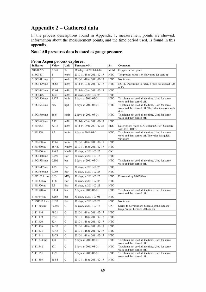
69
Appendix 2 – Gathered data
In the process descriptions found in Appendix 1, measurement points are showed. Information about the measurement points, and the time period used, is found in this appendix.
Note! All pressures data is stated as gauge pressure
From Aspen process explorer: Indicator Value Unit Time period* At: Comment
60A10705 3.648 % 365 days, at 2011-04-14 VCM Oxygen in flue gases
61FC1401 1 ton/h 2010-11-18 to 2011-02-17 HTC The present value is 0. Only used for start-up
61FC1411:me 0 ton/h 2010-11-18 to 2011-02-17 HTC Not in use
61FC1429:me 86.65 m3/h 2011-01-03 to 2011-02-17 HTC NOTE! According to Peter, it must not exceed 120 m3/h
61FC1442:me 12.64 m3/h 2011-01-03 to 2011-02-17 HTC
61FC1445 12.2 m3/h 40 days, at 2011-02-23 HTC 61FC1506:me 4.975 l/min 2 days, at 2011-03-01 HTC Tricolumn not used all the time. Used for some
week and then turned off. 61FC1543:me 306 kg/h 2 days, at 2011-03-01 HTC Tricolumn not used all the time. Used for some
week and then turned off. The value increases with time
61FC1560:me 16.6 l/min 2 days, at 2011-03-01 HTC Tricolumn not used all the time. Used for some week and then turned off.
61FC1645:me 3.12 m3/h 2011-01-03 to 2011-02-17 HTC
61FI1063 32.15 m3/h 2011-01-09 to 2001-02-21 EDC Description: "Feed EDC-column C103" Compare with C61FI1063.
61FI1559 1.2 l/min 1 day, at 2011-03-01 HTC Tricolumn not used all the time. Used for some week and then turned off. The value has quick variations
61FI1608:av 17.65 l/min 2010-11-18 to 2011-02-17 HTC
61FI1630:av 187.49 Nm3/h 2010-11-18 to 2011-02-17 HTC
61FI1630:av 146.2 Nm3/h 30 days, at 2011-02-23 OXI
61PC1448:me 0.296 Bar 30 days, at 2011-03-16 HTC
61PC1558:me 0.102 bar 2 days, at 2011-03-01 HTC Tricolumn not used all the time. Used for some week and then turned off.
61PC1617:me 1.25 Bar 30 days, at 2011-02-23 HTC
61PC1640:me 0.095 Bar 30 days, at 2011-02-23 HTC
61PD1625.1:av 0.03 MVp 30 days, at 2011-02-23 HTC Pressure drop 0,0029 bar
61PI1302:av 17.8 Bar 30 days, at 2011-02-23 HTC
61PI1326:av 2.5 Bar 30 days, at 2011-02-23 HTC
61PI1540:av 0.114 bar 2 days, at 2011-03-01 HTC Tricolumn not used all the time. Used for some week and then turned off.
61PI1644:av 4.265 bar 30 days, at 2011-03-01 HTC
61PS1316.1:av 0.037 Bar 30 days, at 2011-02-23 HTC Not in use
61TI1306:av -0.395 C 30 days, at 2011-03-16 OXI Seems to be variations because of the outdoor temp. Varies between -10 and 25
61TI1416 99.21 C 2010-11-18 to 2011-02-17 HTC
61TI1419 89.2 C 2010-11-18 to 2011-02-17 HTC
61TI1420 82.4 C 2010-11-18 to 2011-02-17 HTC
61TI1426 74.37 C 2010-11-18 to 2011-02-17 HTC
61TI1431 73.45 C 2010-11-18 to 2011-02-17 HTC
61TI1441 26.73 C 2010-11-18 to 2011-02-17 HTC
61TI1538:me 118 C 2 days, at 2011-03-01 HTC Tricolumn not used all the time. Used for some week and then turned off.
61TI1542 87.1 C 2 days, at 2011-03-01 HTC Tricolumn not used all the time. Used for some week and then turned off.
61TI1551 13.9 C 2 days, at 2011-03-01 HTC Tricolumn not used all the time. Used for some week and then turned off.
61TI1603 15.84 C 2010-11-18 to 2011-02-17 HTC

70
61TI1618:me -16.5 C 2010-11-18 to 2011-02-17 HTC
61TI1646:av 57.49 C 2011-01-03 to 2011-02-17 HTC High?
61TI1701 52.8 C 30 days, at 2011-02-25 VCM
61TI1712 85.58 C 2011-01-09 to 2011-02-21 EDC
61TI1714 127.73 C 2011-01-09 to 2011-02-21 EDC
61TI1716 89.32 C 2011-01-09 to 2011-02-21 EDC
61TI1718 111.05 C 2011-01-09 to 2011-02-21 EDC
61TI1721 87.86 C 2011-01-09 to 2011-02-21 EDC irregular data has been removed
61TI1722 92.91 C 2011-01-09 to 2011-02-21 EDC irregular data has been removed
61TI1725 139.6 C 30 days, at 2011-03-16 EDC
62FC2048:me 2.51 m3/h 30 days, at 2011-03-01 VCM
62FC2059:me 37.91 m3/h 2011-01-03 to 2011-02-17 VCM
62FC2075:me 0.56 m3/h 2010-11-18 to 2011-02-17 VCM
62FC2076:me 2801.62 kg/h 2011-01-03 to 2011-02-17 VCM
62FC2102:me 36.48 m3/h 2010-11-18 to 2011-02-17 VCM
62FC2106:me 10.96 m3/h 2010-11-18 to 2011-02-17 VCM
62FC2413:me 7.36 ton/h 2011-01-03 to 2011-02-17 VCM
62FC2415:me 11630.36 Nm3/h 2011-01-03 to 2011-02-17 VCM
62FC2431:me 0.32 ton/h 2011-01-03 to 2011-02-17 VCM Step functions.
62FC2443:me 0.3 m3/h 2010-11-18 to 2011-02-17 VCM Goes up to 0,33 stays, and then goes down quickly again
62FC2461:me 37.94 m3/h 2011-01-03 to 2011-02-17 VCM
62FI2044 0.661 m3/h 30 days at 2011-03-25 VCM
62FI2109 16.45 m3/h 2010-11-18 to 2011-02-17 VCM
62FI2115 0.823 ton/h 2010-11-18 to 2011-02-17 VCM
62FI2216 4215.3 kg/h 2011-01-03 to 2011-02-17 VCM
62FI2220 22.75 m3/h 2011-01-03 to 2011-02-17 VCM
62FI2403 45.13 m3/h 2011-01-03 to 2011-02-17 VCM
62FQ2133 19.45 ton/h 2011-01-03 to 2011-02-17 VCM
62PC2007:me 23 Bar 30 days, at 2011-02-23 VCM
62PC2069:me 9.1 Bar 30 days, at 2011-02-23 VCM
62PC2073:me 0.6 Bar 30 days, at 2011-02-23 VCM
62PC2117:me 5.0 Bar 30 days, at 2011-02-23 VCM
62PD2121 0.55 Bar 30 days, at 2011-02-23 VCM
62PI2046 9.6 Bar 30 days, at 2011-02-23 VCM
62PI2246 10.25 Bar 15 days, at 2011-02-23 VCM
62PI2247 9.0 Bar 30 days, at 2011-02-23 OXI
62PI2418 20 Bar 30 days, at 2011-02-23 VCM
62TC2036:me 40 C 2010-11-18 to 2011-02-17 VCM
62TC2414:me 118.12 C 2011-01-03 to 2011-02-17 VCM
62TI2001 486.8 C 2011-01-03 to 2011-02-17 VCM
62TI2002 445.59 C 2011-01-03 to 2011-02-17 VCM
62TI2003 231.33 C 2011-01-03 to 2011-02-17 VCM
62TI2008 193.14 C 2011-01-03 to 2011-02-17 VCM
62TI2018 208.61 C 2011-01-03 to 2011-02-17 VCM
62TI2025D 585.4 C 365 days, at 2011-04-14 VCM
62TI2028 160.91 C 2010-11-18 to 2011-02-17 VCM
62TI2032 127.93 C 2010-11-18 to 2011-02-17 VCM
62TI2033 157.9 C 30 days at 2011-03-25 VCM
62TI2041 20.96 C 2010-11-18 to 2011-02-17 VCM
62TI2042 -32.32 C 2010-11-18 to 2011-02-17 VCM
62TI2043 -31.9 C 30 days, at 2011-03-01 VCM
62TI2047 86.48 C 2011-01-03 to 2011-02-17 VCM
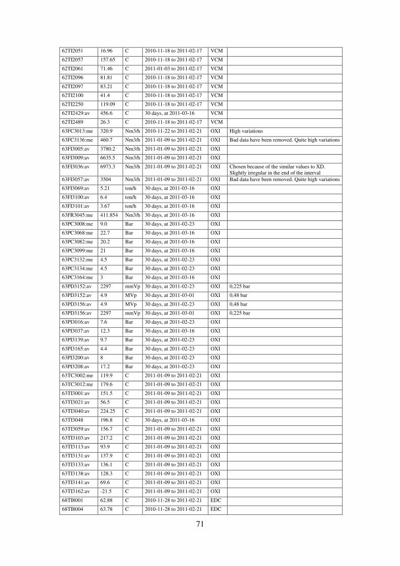
71
62TI2051 16.96 C 2010-11-18 to 2011-02-17 VCM
62TI2057 157.65 C 2010-11-18 to 2011-02-17 VCM
62TI2061 71.46 C 2011-01-03 to 2011-02-17 VCM
62TI2096 81.81 C 2010-11-18 to 2011-02-17 VCM
62TI2097 83.21 C 2010-11-18 to 2011-02-17 VCM
62TI2100 41.4 C 2010-11-18 to 2011-02-17 VCM
62TI2250 119.09 C 2010-11-18 to 2011-02-17 VCM
62TI2429:av 456.6 C 30 days, at 2011-03-16 VCM
62TI2489 26.3 C 2010-11-18 to 2011-02-17 VCM
63FC3013:me 320.9 Nm3/h 2010-11-22 to 2011-02-21 OXI High variations
63FC3136:me 460.7 Nm3/h 2011-01-09 to 2011-02-21 OXI Bad data have been removed. Quite high variations
63FI3005:av 3780.2 Nm3/h 2011-01-09 to 2011-02-21 OXI
63FI3009:av 6635.5 Nm3/h 2011-01-09 to 2011-02-21 OXI
63FI3036:av 6973.3 Nm3/h 2011-01-09 to 2011-02-21 OXI Chosen because of the similar values to XD. Slightly irregular in the end of the interval
63FI3057:av 3504 Nm3/h 2011-01-09 to 2011-02-21 OXI Bad data have been removed. Quite high variations
63FI3069:av 5.21 ton/h 30 days, at 2011-03-16 OXI
63FI3100:av 6.4 ton/h 30 days, at 2011-03-16 OXI
63FI3101:av 3.67 ton/h 30 days, at 2011-03-16 OXI
63FR3045:me 411.854 Nm3/h 30 days, at 2011-03-16 OXI
63PC3008:me 9.0 Bar 30 days, at 2011-02-23 OXI
63PC3068:me 22.7 Bar 30 days, at 2011-03-16 OXI
63PC3082:me 20.2 Bar 30 days, at 2011-03-16 OXI
63PC3099:me 21 Bar 30 days, at 2011-03-16 OXI
63PC3132:me 4.5 Bar 30 days, at 2011-02-23 OXI
63PC3134:me 4.5 Bar 30 days, at 2011-02-23 OXI
63PC3164:me 3 Bar 30 days, at 2011-03-16 OXI
63PD3152:av 2297 mmVp 30 days, at 2011-02-23 OXI 0,225 bar
63PD3152:av 4.9 MVp 30 days, at 2011-03-01 OXI 0,48 bar
63PD3156:av 4.9 MVp 30 days, at 2011-02-23 OXI 0,48 bar
63PD3156:av 2297 mmVp 30 days, at 2011-03-01 OXI 0,225 bar
63PI3016:av 7.6 Bar 30 days, at 2011-02-23 OXI
63PI3037:av 12.3 Bar 30 days, at 2011-03-16 OXI
63PI3139:av 9.7 Bar 30 days, at 2011-02-23 OXI
63PI3165:av 4.4 Bar 30 days, at 2011-02-23 OXI
63PI3200:av 8 Bar 30 days, at 2011-02-23 OXI
63PI3208:av 17.2 Bar 30 days, at 2011-02-23 OXI
63TC3002:me 119.9 C 2011-01-09 to 2011-02-21 OXI
63TC3012:me 179.6 C 2011-01-09 to 2011-02-21 OXI
63TI3001:av 151.5 C 2011-01-09 to 2011-02-21 OXI
63TI3021:av 56.5 C 2011-01-09 to 2011-02-21 OXI
63TI3040:av 224.25 C 2011-01-09 to 2011-02-21 OXI
63TI3048 196.8 C 30 days, at 2011-03-16 OXI
63TI3059:av 156.7 C 2011-01-09 to 2011-02-21 OXI
63TI3103:av 217.2 C 2011-01-09 to 2011-02-21 OXI
63TI3113:av 93.9 C 2011-01-09 to 2011-02-21 OXI
63TI3131:av 137.9 C 2011-01-09 to 2011-02-21 OXI
63TI3133:av 136.1 C 2011-01-09 to 2011-02-21 OXI
63TI3138:av 128.3 C 2011-01-09 to 2011-02-21 OXI
63TI3141:av 69.6 C 2011-01-09 to 2011-02-21 OXI
63TI3162:av -21.5 C 2011-01-09 to 2011-02-21 OXI
68TI8001 62.88 C 2010-11-28 to 2011-02-21 EDC
68TI8004 63.78 C 2010-11-28 to 2011-02-21 EDC
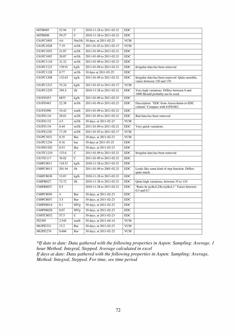
72
68TI8005 52.94 C 2010-11-28 to 2011-02-21 EDC
68TI8008 59.27 C 2010-11-28 to 2011-02-21 EDC
C61FC1003 4.6 Nm3/h 30 days, at 2011-02-25 VCM
C61FC1028 7.19 m3/h 2011-01-03 to 2011-02-17 VCM
C61FC1052 21.87 m3/h 2011-01-09 to 2011-02-21 EDC
C61FC1092 20.07 m3/h 2011-01-09 to 2011-02-21 EDC
C61FC1118 21.22 m3/h 2011-01-09 to 2011-02-21 EDC
C61FC1123 139.91 kg/h 2011-01-09 to 2011-02-21 EDC Irregular data has been removed
C61FC1128 0.77 m3/h 30 days at 2011-03-25 EDC
C61FC1208 132.63 kg/h 2011-01-09 to 2011-02-21 EDC Irregular data has been removed. Quite unstable, varies between 120 and 170
C61FC1223 35.24 kg/h 2011-01-03 to 2011-02-17 VCM
C61FC1229 394.4 l/h 2010-11-28 to 2011-02-21 EDC Very high variations. Differs between 0 and 1000.Should probably not be used.
C61FI1053 6833 kg/h 2011-01-09 to 2011-02-21 EDC
C61FI1063 22.38 m3/h 2011-01-09 to 2011-02-21 EDC Description: "EDC from Azeocolumn to EDC column" Compare with 61FI1063.
C61FI1096 10.42 ton/h 2011-01-09 to 2011-02-21 EDC
C61FI1116 28.01 m3/h 2011-01-09 to 2011-02-21 EDC Bad data has been removed
C61FI1132 4.5 m3/h 30 days, at 2011-02-23 VCM
C61FI1134 0.44 m3/h 2011-01-09 to 2011-02-21 EDC Very quick variations
C61FS1230 17.29 m3/h 2011-01-03 to 2011-02-17 VCM
C61PC1031 0.35 Bar 30 days, at 2011-02-23 VCM
C61PC1236 0.16 bar 30 days at 2011-03-25 EDC
C61PD1202 0.53 Bar 30 days, at 2011-02-23 EDC
C61TC1210 133.6 C 2011-01-09 to 2011-02-21 EDC Irregular data has been removed
C61TI1117 36.02 C 2011-01-09 to 2011-02-21 EDC
C68FC8011 118.51 kg/h 2010-11-28 to 2011-02-21 EDC
C68FC8013 201.94 l/h 2011-01-09 to 2001-02-21 EDC Looks like some kind of step function. Differs quite much.
C68FC8030 33.87 kg/h 2010-11-28 to 2011-02-21 EDC
C68FI8027 72.72 l/h 2010-11-28 to 2011-02-21 EDC Quite high variations, between 35 to 110
C68FR8027 0.5 2010-11-28 to 2011-02-21 EDC "Ratio In etylkol.2/In etylkol.1" Varies between 0,3 and 0,7
C68PC8056 4 Bar 30 days, at 2011-02-23 EDC
C68PC8057 3.5 Bar 30 days, at 2011-02-23 EDC
C68PD8014 0.1 MVp 30 days, at 2011-02-23 EDC
C68PD8028 0.07 MVp 30 days, at 2011-02-23 EDC
C68TC8032 57.5 C 30 days, at 2011-02-23 EDC
FI2309 2.545 ton/h 30 days, at 2011-04-14 VCM
H62PI2221 15.2 Bar 30 days, at 2011-02-23 VCM
H62PI2270 0.606 Bar 30 days, at 2011-02-25 VCM
*If date to date: Data gathered with the following properties in Aspen: Sampling: Average, 1 hour Method: Integral, Stepped. Average calculated in excel If days at date: Data gathered with the following properties in Aspen: Sampling: Average, Method: Integral, Stepped. For time, see time period

73
Data from local measurement points:
Name of unit: At: Number of point
Value Unit Description Date Outdoor temp:
615- S103 EDC PI1014/1015 6 bar Pressure after pump after S103 28-feb ca 0 C
615-C102 EDC PI1008+1009 14 bar Pressure after pump, inlet stream Azeocolumn
15-mar ca 5 C
615-C102 EDC PI1010+1011 2.9 bar Pressure after pump, bottom outlet Azeocolumn
15-mar ca 5 C
615-C102 EDC PI1033 2.4 bar Pressure bottom Azeo column 28-feb ca 0 C
615-C105 EDC PI1048 0.4 bar Pressure Tri-column 28-feb ca 0 C
615-H106 EDC PI1036 2 bar Pressure top Azeo column/ in EDC condenser
28-feb ca 0 C
615-H106 EDC TI2003 15 C Temp. outgoing cooling water EDC condenser H106
28-feb ca 0 C
615-H109 EDC PI1040 0.2 bar Pressure in EDC-condenser and out from top EDC column
28-feb ca 0 C
615-H109 EDC TI2002 26 C Temp. outgoing cooling water EDC condenser H109
28-feb ca 0 C
615-S102 EDC PI1013 10 bar Pressure after pump after S102 28-feb ca 0 C
615-S102 EDC PI1037 2 bar Pressure distillate tank S102 28-feb ca 0 C
685-09 EDC PI1001 2 bar Pressure tank 685-09 28-feb ca 0 C
615-C151 HTC PI1111+1112 5.5 bar Pressure after pump, bottom HTC-column
28-feb ca 0 C
615-C151 HTC PI1114 0.5 bar Pressure HTC column 15-mar ca 5 C
615-H153 HTC TI2018 68 C Temperature outgoing cooling water condenser H153
28-feb ca 0 C
615-H154 HTC TI2015 16 C Temperature outgoing cooling water condenser H154
28-feb ca 0 C
615-H159 HTC TI2013 12 C Temperature outgoing cooling water from cooler H159
28-feb ca 0 C
615-H160 HTC TI2020 15 C Temperature outgoing cooling water from cooler H160
28-feb ca 0 C
615-H166 HTC TI2023 34 C Temperature outgoing stream from H166
28-feb ca 0 C
615-S151 HTC PI1115 0.1 bar Pressure S151 15-mar ca 5 C
615-S151 HTC PI1116+1117 7 bar Pressure after pump after S151 15-mar ca 5 C
615-S152 HTC PI1126 0.1 bar Pressure EDC-separator S152 28-feb ca 0 C
615-S156 HTC PI1152+1153 5.2 bar Pressure after pump after S156 28-feb ca 0 C
T301 HTC PI1124+1125 1.8 bar Pressure after pump after 615-S152+615-S153
28-feb ca 0 C
635-H303A OXI TI2002 14 C Temperature outgoing cooling water condenser H203A
28-feb ca 0 C
635-H303B OXI TI2001 15.5 C Temperature outgoing cooling water condenser H203B
28-feb ca 0 C
635-H306 OXI PI1027 3.5 bar Pressure in remainder gas condenser H306
28-feb ca 0 C
635-H321 OXI PI1036 2.2 bar Pressure of air going in to intermediate cooler H321
28-feb ca 0 C
635-H321 OXI TI1302 18 C Temperature outgoing cooling water intermediate cooler H321
28-feb ca 0 C
635-H321 OXI TI2007 160 C Temperature of air going in to intermediate cooler H321
28-feb ca 0 C
635-H321 OXI TI2008 25 C Temperature of air going out of intermediate cooler H321
28-feb ca 0 C

74
615-H122 VCM PI1052 2 bar Pressure out H122 28-feb ca 0 C
615-H122 VCM TI2009 60 C Temperature out R102 after 615-H122 = temp. Out of H122
28-feb ca 0 C
615-T101 VCM PI1001+1002 9 bar Pressure after pump after T101 15-mar ca 5 C
625-H202A VCM TI2001 50 C Temperature outgoing cooling water condenser H202A
28-feb ca 0 C
625-H210 VCM TI2002 13 C Temp. outgoing cooling water VCM-tar condenser H210
28-feb ca 0 C
625-H212 VCM PI1008 11.5-12
bar Pressure after pump after 625-T202/ in preheater H212
28-feb ca 0 C
625-S202 VCM PI1006 15 bar Pressure after pump after 625-S202 28-feb ca 0 C
615-H121 VCM + EDC
TI2008 98 C Temperature out cold stream H121 to EDC-column
28-feb ca 0 C
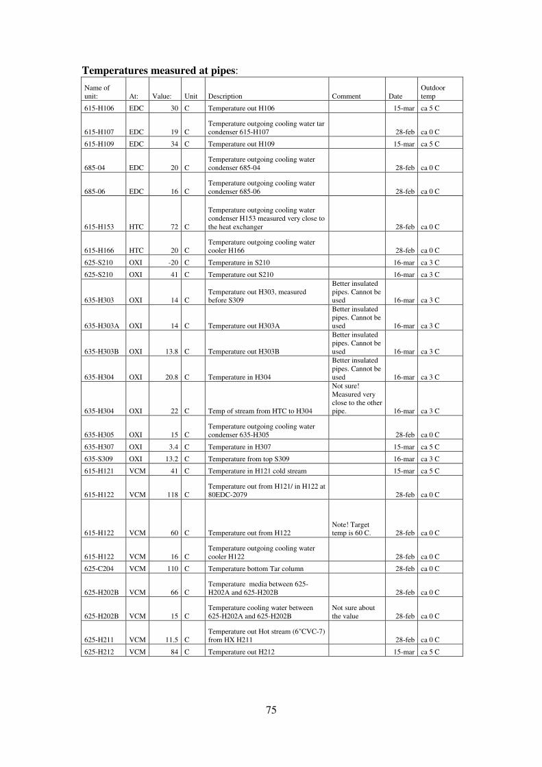
75
Temperatures measured at pipes:
Name of unit: At: Value: Unit Description Comment Date
Outdoor temp
615-H106 EDC 30 C Temperature out H106 15-mar ca 5 C
615-H107 EDC 19 C Temperature outgoing cooling water tar condenser 615-H107 28-feb ca 0 C
615-H109 EDC 34 C Temperature out H109 15-mar ca 5 C
685-04 EDC 20 C Temperature outgoing cooling water condenser 685-04 28-feb ca 0 C
685-06 EDC 16 C Temperature outgoing cooling water condenser 685-06 28-feb ca 0 C
615-H153 HTC 72 C
Temperature outgoing cooling water condenser H153 measured very close to the heat exchanger 28-feb ca 0 C
615-H166 HTC 20 C Temperature outgoing cooling water cooler H166 28-feb ca 0 C
625-S210 OXI -20 C Temperature in S210 16-mar ca 3 C
625-S210 OXI 41 C Temperature out S210 16-mar ca 3 C
635-H303 OXI 14 C Temperature out H303, measured before S309
Better insulated pipes. Cannot be used 16-mar ca 3 C
635-H303A OXI 14 C Temperature out H303A
Better insulated pipes. Cannot be used 16-mar ca 3 C
635-H303B OXI 13.8 C Temperature out H303B
Better insulated pipes. Cannot be used 16-mar ca 3 C
635-H304 OXI 20.8 C Temperature in H304
Better insulated pipes. Cannot be used 16-mar ca 3 C
635-H304 OXI 22 C Temp of stream from HTC to H304
Not sure! Measured very close to the other pipe. 16-mar ca 3 C
635-H305 OXI 15 C Temperature outgoing cooling water condenser 635-H305 28-feb ca 0 C
635-H307 OXI 3.4 C Temperature in H307 15-mar ca 5 C
635-S309 OXI 13.2 C Temperature from top S309 16-mar ca 3 C
615-H121 VCM 41 C Temperature in H121 cold stream 15-mar ca 5 C
615-H122 VCM 118 C Temperature out from H121/ in H122 at 80EDC-2079 28-feb ca 0 C
615-H122 VCM 60 C Temperature out from H122 Note! Target temp is 60 C. 28-feb ca 0 C
615-H122 VCM 16 C Temperature outgoing cooling water cooler H122 28-feb ca 0 C
625-C204 VCM 110 C Temperature bottom Tar column 28-feb ca 0 C
625-H202B VCM 66 C Temperature media between 625-H202A and 625-H202B 28-feb ca 0 C
625-H202B VCM 15 C Temperature cooling water between 625-H202A and 625-H202B
Not sure about the value 28-feb ca 0 C
625-H211 VCM 11.5 C Temperature out Hot stream (6"CVC-7) from HX H211 28-feb ca 0 C
625-H212 VCM 84 C Temperature out H212 15-mar ca 5 C

76
LabMaster data
Na
me
of
un
itD
esc
rip
tio
nS
ub
sta
ns
Me
an
Va
lue
Un
itS
ub
sta
ns
Me
an
Va
lue
Un
itS
ub
sta
ns
Me
an
Va
lue
Un
itS
ub
sta
ns
Me
an
Va
lue
Un
itS
ub
sta
ns
Me
an
Va
lue
Un
itS
ub
sta
ns
Me
an
Va
lue
Un
itS
ub
sta
ns
Me
an
Va
lue
Un
it
61
5-C
10
2A
zeo
-co
lum
n b
ott
om
ED
C9
9,2
Ma
ss
%1
.1.2
Trik
lore
tan
35
31
ViP
PM
61
5-C
10
2A
zeo
-co
lum
n t
op
Klo
rofo
rm3
8,1
Ma
ss
%E
thy
len
e c
hlo
rid
e2
9,1
Ma
ss
%T
r1.2
dik
lore
ten
10
,7M
ass
%1
.1d
iklo
reta
n5
,7m
as
s%
cis
1.2
dik
lore
ten
4,9
Ma
ss
%V
CM
2,8
Ma
ss%
Ko
lte
tra
klo
rid
4,4
Ma
ss
%
61
5-C
10
2
Fe
ed
in
to E
DC
-cle
an
ing
ED
C9
7,9
Ma
ss
%E
tylk
lori
d4
05
2V
iPP
MK
loro
form
45
50
ViP
PM
1.1
.2T
rik
lore
tan
33
02
ViP
PM
61
5-C
10
3E
DC
-co
lum
n b
ott
om
ED
C6
5,7
Ma
ss
%1
.1.2
Trik
lore
tan
15
,7M
as
s%
Te
tra
klo
reta
n1
,9M
ass
%P
en
tak
lore
tan
2,7
Ma
ss
%B
rom
trik
lore
tan
1,3
Ma
ss
%
61
5-C
10
3E
DC
-co
lum
n t
op
ED
C9
9,4
5M
as
s%
Ko
lte
tra
klo
rid
25
75
ViP
PM
Tri
klo
rete
n1
36
6V
iPP
MB
en
se
n1
00
0V
iPP
M
61
5-C
10
5E
DC
tri
colu
mn
1.1
.2T
rik
lore
tan
50
,7M
as
s%
ED
C6
,5M
as
s%
Te
tra
klo
reta
n6
Ma
ss%
Pe
nta
klo
reta
n8
,5m
as
s%
Bro
mtr
iklo
reta
n3
,4M
as
s%
He
xa
klo
reta
n1
,9M
as
s%
61
5-C
10
5E
DC
tri
colu
mn
ED
C9
9,1
Ma
ss
%1
.1.2
Trik
lore
tan
1M
as
s%
61
5-C
15
1H
TC
-co
lum
n b
ott
om
ED
C8
3,2
Ma
ss
%1
.1.2
Trik
lore
tan
14
,6M
as
s%
1B
rom
2K
lore
tan
1,7
Ma
ss%
61
5-C
15
2H
TC
tri
colu
mn
ED
C9
8,3
Ma
ss
%1
Bro
m2
Klo
reta
n0
,5M
as
s%
1.1
.2T
rik
lore
tan
1,1
Ma
ss%
61
5-C
15
2H
TC
tri
colu
mn
1.1
.2T
rik
lore
tan
80
,5M
as
s%
ED
C9
,2M
as
s%
1B
rom
2K
lore
tan
6,7
Ma
ss%
Te
tra
klo
reta
n5
,1m
as
s%
61
5-R
15
1H
TC
-re
act
or
ED
C5
9,3
Ma
ss
%1
.1.2
Trik
lore
tan
18
,5M
as
s%
1B
rom
2K
lore
tan
2,7
Ma
ss%
Te
tra
klo
reta
n1
,8m
as
s%
61
5-S
15
1H
TC
de
stil
late
ta
nk
ED
C9
9,9
Ma
ss
%
61
5-S
15
2 +
61
5-S
15
3H
TC
ED
C-s
ep
ara
tor
ED
C9
9,8
5M
as
s%
Ete
n4
71
ViP
PM
61
5-S
15
3H
TC
ve
nt.
Ga
sK
vä
ve
68
,6V
ol%
Ete
n2
4,3
1V
ol%
Eta
n1
Vo
l%E
DC
1V
ol%
Sy
re3
,7V
ol%
62
5-C
20
2H
Cl
colu
mn
to
pH
Cl
99
,7V
ol%
62
5-C
20
3V
CM
co
lum
n b
ott
om
ED
C9
8,5
Ma
ss
%K
olt
etr
ak
lori
d5
38
6V
iPP
M
62
5-H
21
3
Fe
ed
to
R2
01
ED
C9
9,6
Ma
ss
%K
olt
etr
ak
lori
d2
03
0V
iPP
M
63
5-S
30
6O
XI
ED
C-s
ep
ara
tor
ED
C9
8,5
Ma
ss
%E
tylk
lori
d3
83
0V
iPP
MK
lora
l3
46
9V
iPP
M
63
5-S
30
7O
XI
ED
C f
ina
l se
pa
rato
rE
DC
97
,1M
as
s%
Ety
lklo
rid
18
55
3V
iPP
MT
r1.2
dik
lore
ten
29
80
ViP
PM
63
5-S
30
9O
XI
ED
C-s
ep
ara
tor
ED
C9
8,2
Ma
ss
%E
tylk
lori
d4
44
0V
iPP
M1
.1.2
Tri
klo
reta
n3
76
6V
iPP
M
68
5-0
1E
tCl
colu
mn
1 b
ott
om
Klo
rofo
rm5
4,8
Ma
ss
%tr
1.2
Dik
lore
ten
14
,8M
as
s%
1.1
Dik
lore
tan
7,6
Ma
ss%
cis
1.2
Dik
lore
ten
6,9
Ma
ss
%K
olt
etr
ak
lori
d6
,4M
as
s%
Ety
lklo
rid
5,5
Ma
ss%
68
5-0
2E
tCl
colu
mn
2 b
ott
om
Ety
lklo
rid
98
,4M
as
s%
Ete
no
xid
15
63
1V
iPP
M

77
Appendix 3 - Calculations of composition and flow rate
leaving Oxi-reactors
The flow rate and composition out from the Oxi-reactors are not measured. In this appendix, calculations are done based on the ingoing substances to the reactors.
R301-R303
Inlet flow of substances to reactor 1-3:
Component Volume flow into
reactor R301-R303
[Nm3/h] (from
gathered data)
Mole flow[mol/s]
(from Aspen plus)
Measurement point
Ethylene 3780.2 42.35994 63FI3005 HCl 6635.5 74.35481 63FI3009 Air 6973.3 78.14007 63FI3036 Air-nitrogen 61.7306553 Air-oxygen 16.4094147 Oxygen 411.85 4.61503 63FR3045 Total oxygen flow 21.0244447
Reaction: C2H4+2HCl+½O2 → C2H4Cl2+H2O All HCl is assumed to react. However, some will dissolve into water, and hydrochloric acid with a concentration of 8% is leaving the Oxi-reactors. Reactions: For 1 mole of HCl reacted; Needed: Ethylene ½ mole Oxygen 1/4 mole Produced: EDC ½ mole Water ½ mole Dissolved* HCl 0.0438
*8% HCl-acid out
In the following table, the outlet concentrations are calculated
Outlet concentrations and flow rate from R303:
Compound: In to R301-
R303[mol/s]
Change
[mol/s]
Dissolved [mol/s]
Out from
R303[mol/s]
Molefraction out
HCl 74.355 -71.257 -3.098 0.000 0,000 Ethylene 42.360 -35.628 6.732 0,046 Nitrogen 61.731 0.000 61.731 0,423 Oxygen 21.024 -17.814 3.210 0,022
EDC 0.000 35.628 35.628 0,244 Water 0.000 35.628 35.628 0,244 Dissolved HCl 3.098 3.098 0,021 Total mole flow: 146.027

78
R304
The flow consists of two parts. Chlorine from a chlorine evaporator, where the flow is measured, and a flow from a separator after the first three reactors, which had to be simulated in Aspen plus. Reaction: C2H4+Cl2→C2H4Cl2
Outlet concentrations and flow rate from R304:
From 63FC3135: Into R304 from H307:
Compound: In to R304 [mol/s]
Change [mol/s]
Out from R304[mol/s]
Chlorine 5.162 -5.162 0.000 0.000 From Aspen simulations:
Into reactor R304 from H304:
Compound: In to R304 [mol/s]
Change [mol/s]
Out from R304 [mol/s]
Molefraction
Ethylene 5.931 -5.162 0.769 0.011 EDC 0.864 5.162 6.026 0.085 Water 0.122 0.000 0.122 0.002 Oxygen 3.264 0.000 3.264 0.046 Nitrogen 62.880 0.000 62.880 0.890 Ethane 0.016 0.000 0.016 0.000 Total mole
flow: 73.0775811
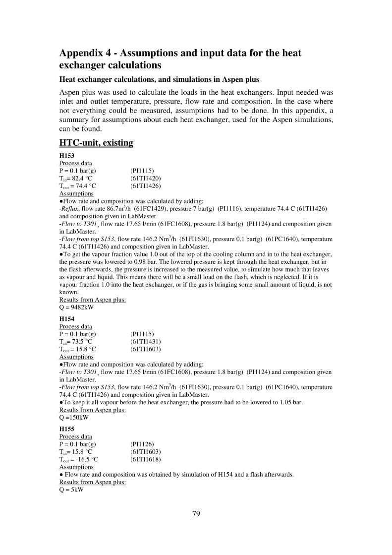
79
Appendix 4 - Assumptions and input data for the heat
exchanger calculations
Heat exchanger calculations, and simulations in Aspen plus
Aspen plus was used to calculate the loads in the heat exchangers. Input needed was inlet and outlet temperature, pressure, flow rate and composition. In the case where not everything could be measured, assumptions had to be done. In this appendix, a summary for assumptions about each heat exchanger, used for the Aspen simulations, can be found.
HTC-unit, existing
H153 Process data P = 0.1 bar(g) (PI1115) Tin= 82.4 °C (61TI1420) Tout = 74.4 °C (61TI1426) Assumptions ●Flow rate and composition was calculated by adding: -Reflux, flow rate 86.7m3/h (61FC1429), pressure 7 bar(g) (PI1116), temperature 74.4 C (61TI1426) and composition given in LabMaster. -Flow to T301¸ flow rate 17.65 l/min (61FC1608), pressure 1.8 bar(g) (PI1124) and composition given in LabMaster. -Flow from top S153, flow rate 146.2 Nm3/h (61FI1630), pressure 0.1 bar(g) (61PC1640), temperature 74.4 C (61TI1426) and composition given in LabMaster. ●To get the vapour fraction value 1.0 out of the top of the cooling column and in to the heat exchanger, the pressure was lowered to 0.98 bar. The lowered pressure is kept through the heat exchanger, but in the flash afterwards, the pressure is increased to the measured value, to simulate how much that leaves as vapour and liquid. This means there will be a small load on the flash, which is neglected. If it is vapour fraction 1.0 into the heat exchanger, or if the gas is bringing some small amount of liquid, is not known. Results from Aspen plus: Q = 9482kW
H154
Process data P = 0.1 bar(g) (PI1115) Tin= 73.5 °C (61TI1431) Tout = 15.8 °C (61TI1603) Assumptions ●Flow rate and composition was calculated by adding: -Flow to T301¸ flow rate 17.65 l/min (61FC1608), pressure 1.8 bar(g) (PI1124) and composition given in LabMaster. -Flow from top S153, flow rate 146.2 Nm3/h (61FI1630), pressure 0.1 bar(g) (61PC1640), temperature 74.4 C (61TI1426) and composition given in LabMaster. ●To keep it all vapour before the heat exchanger, the pressure had to be lowered to 1.05 bar. Results from Aspen plus: Q =150kW
H155
Process data P = 0.1 bar(g) (PI1126) Tin= 15.8 °C (61TI1603) Tout = -16.5 °C (61TI1618) Assumptions ● Flow rate and composition was obtained by simulation of H154 and a flash afterwards. Results from Aspen plus: Q = 5kW

80
H158AB
Process data P= 0.1 bar(g) in middle of column (61PI1540) Tin= 118 °C (61TI1538) Composition from LabMaster m¦ 2 /40=306 kg/h (61FC1543) -Only run 1/3 of the time Assumptions ●Pressure set to 1.3 bar to obtain saturated liquid in. ●Assuming saturated vapour out. ●1-bromo-2-chloro-ethane does not exist in the Aspen database. It was approximated with 50% C2H4Cl2 and 50% C2H4Br2
Results from Aspen plus: Q=170 kW Tout = 123.5 °C
H159
Process data P= 0.1 bar(g) in middle of column (61PI1540) Tin= 87.1 °C (61TI1542) Tout = 13.9 °C (61TI1551) Composition from LabMaster -Only run 1/3 of the time Assumptions ●Flow rate was calculated by adding: -Reflux, flow rate 16,6 l/min (61FC1560) and pressure 5.2 bar(g) (PI1152), - Return HTC reactor, flow rate 1.2 l/min (61FI1559) and pressure 5.2 bar(g) (PI1152) Results from Aspen plus: Q=157 kW
H160
Process data P= 0.3 bar(g) after cooler (61PC1448) Tin= 89.2 °C (61TI1419) Tout = 26.7 °C (61TI1441) Flow rate=12.6 m3/h (61FC1442) Assumptions ●Composition: Pure EDC Results from Aspen plus: Q = 364 kW
H166
Process data P= 4.3 bar(g) after S184 (61PI1644) Tin= 57.5 °C (61TI1646) Tout = 34 °C (TI2023) Flow rate=3.12 m3/h (61FC1645) Composition from LabMaster Results from Aspen plus: Q = 33kW
HTC-unit, future
No temperatures or pressures are assumed to change in the future, but will be the same as in the previous calculations for the present HTC unit.
As mentioned, the reflux is limited, and cannot increase by more than 38%. However, the production of light products is assumed to be doubled, like the production of all other products. This means that a new steady-state is assumed to be reached, with a slightly higher content of volatile compounds in the stream leaving the top of the HTC-column. Since the HTC-condenser is substantially larger than the following coolers, it is possible for the reflux to increase by only 38%, and the mass flow through the

81
following coolers to increase with 100%. The increased flow in the other heat exchangers will barely increase the load of the HTC-condenser, which increases with about 38%.
H153
Current load Q = 9482kW Assumptions As mentioned, the reflux is limited, and cannot increase by more than 38%. However, the production of light products is assumed to be doubled, like the production of all other products. This means that a new steady-state is assumed to be reached, with a slightly higher content of volatile compounds in the stream leaving the top of the HTC-column. Since the HTC-condenser is substantially larger than the following coolers, it is possible for the reflux to increase by only 38%, and the mass flow through the following coolers to increase with 100%. The increased flow in the other heat exchangers will barely increase the load of the HTC-condenser, which increases with about 38%. Future load Q=13065kW
H154
Current load Q=150 kW Assumptions Load doubled. See assumptions for H153. Future load Q=300kW
H155
Current load Q=5 kW Assumptions Load doubled. See assumptions for H153. Future load Q=10kW
H158AB
Current load Q=170 kW Assumptions ●Today, it is only running 1/3 of the time. In the future, when the production is doubled, it is assumed to be running continuously, but at 2/3 of today’s level. Future load Q=114 kW
H159
Current load Q=157 kW Assumptions ●Today, it is only running 1/3 of the time. In the future, when the production is doubled, it is assumed to be running continuously, but at 2/3 of today’s level. Future load Q=104 kW
H160
Current load Q=364 kW Assumptions Production doubled. However, after discussion with the company, the flow rate is expected to increase to 35 m3/h in the future Future load Q=1011kW
H166 Current load Q =33 kW

82
Assumptions Load doubled. See assumptions for H153 Future load Q =65 kW
New started heat exchangers not in use today:
H164
●Simulated in Aspen Exchanger design and rating. The simulations were based on an information sheet for the heat exchanger. The results are very insecure, but will not affect the result since the additional load is placed on Hnew ●Assumed inlet temperature: 100°C ●Assumed outlet temperature: 40°C Future load 1200 kW
H165 ●Simulated in Aspen Exchanger design and rating. The simulations were based on an information sheet for the heat exchanger. The results are very insecure, but will not affect the result since the additional load is placed on Hnew ●Assumed inlet temperature: 115 °C ●Assumed outlet temperature: 40 °C Future load 1600 kW
Hnew
●Calculated by doubling the load of the current H153, and subtracting the load for the future H153, H164 and H165 ●Assumed inlet temperature: 100 °C ●Assumed outlet temperature: 40 °C Future load 3099 kW
VCM-unit
H121
Process data Hot side: P= 5.5 bar(g) (62PC2117+62PD2121) Tin= 157.7 °C (62TI2057) Tout = 118 °C (Measured at pipe) Flow rate=16.45 m3/h (62FI2109) Composition from LabMaster, VCM column bottom Cold side: P= 9 bar(g) (PI1001) Tin= 41 °C (Measured at pipe) Tout = 98 °C (TI2008) Flow rate=7.2 m3/h (C61FC1028) Composition unknown Assumptions ●Bad agreement between the hot and the cold side of the heat exchanger. The load is determined from the hot side, since the data measured are closer to the heat exchanger, and are believed to be more trustworthy. Results from Aspen plus: Q=300 kW
H122 Process data P= 5.5 bar(g) (62PC2117+62PD2121) Tin= 118 °C (Measured at pipe) Tout = 60 °C (TI2009 after R102) Flow rate=16.45 m3/h (62FI2109) Composition from LabMaster, VCM column bottom
83
Assumptions ●Same flow rate as in H121 assumed, even though the flow rate measured after the heat exchanger is larger. Results from Aspen plus: Q=389 kW
H201
Process data Pin= 20 bar(g) (62PI2418) Pout= 15.2 bar(g) (H62PI1221) Tin= 193.1 °C (62TI2008) Tout =208.61 °C (62TI2018) Composition from LabMaster, Feed to R201 Assumptions ●Flow rate calculated by adding 11630 Nm3/h (62FI2109) to cracker and 2.51 m3/h (62FC2048) to C103. ●The flow to C103 is assumed to have same pressure as the outlet stream to the cracker, but is assumed to leave as liquid, and therefore at a temperature of 207.5 °C Results from Aspen plus: Q=3442 kW
H202A Process data P= 10.25 bar(g) (62PI2246) Tin= 127.9 °C (62TI2032) Tout = 66 °C (Measured at pipe) Assumptions ●The condensers and the cooling column tank afterwards were modeled. The condensate flow rate was calculated by adding 37.9 m3/h (62FC2059) to the cooling column and 37.9 m3/h (62FC2461) to the HCl-column. The flow rate in the condensers was set to obtain the calculated condensate flow. ●The composition is unknown. It is taken from the old Aspen simulation, made in 2001, and is changed slightly because of a mass balance made for ingoing and outgoing HCl to the HCl-column ●Pressure lowered to 10 bar(g), and temperature increased to 132.8 C, to obtain vapour fraction 1. Results from Aspen plus: Q=7007 kW
H202B
Process data P= 10.25 bar(g) (62PI2246) Tin= 66°C (Measured at pipe) Tout = 40°C (62TC2036) Assumptions ●The same assumptions as for H202A Results from Aspen plus: Q=2098 kW
H204
Process data P= 9.1 bar(g) (62PC2117+62PD2121) Tout =-32.3°C (62TI2042) Composition from LabMaster, HCl column top Flow rate propene=22.75 m3/h (62FI2220) Pressure propene=0.6 bar(g) (62PC2073) Assumptions ●The load is calculated by assuming all propene liquid, and vapour out. ●The inlet temperature is set to obtain vapour fraction 1.0 in. Results from Aspen plus: Tout =-31.7°C Q =1640kW
H205
Process data

84
Pin= 9.6 bar(g) (62PI2046) Tin= 86.5°C (62TI2047) Flow rate of 10bar steam: 2.8 ton/h (62FC2076) Assumptions ●Composition calculated in Aspen plus from the fact that it should be saturated liquid in, and the mixture should contain only EDC and VCM ●Outlet temperature calculated, assuming vapour fraction 1 for the stream leaving the reboiler ●The load calculated from the condensation heat in the steam Results from Aspen plus: Q=1559 kW Tout= 145°C
H206
Process data P= 5.5 bar(g) (62PC2117+62PD2121) Tin= 157.7 °C (62TI2057) Composition from LabMaster, VCM column bottom Flow rate of 20bar steam: 4.22 ton/h (62FI2216) Assumptions ●Outlet temperature is calculated, assuming vapour fraction 1.0 for the stream leaving the reboiler ●The load is calculated from the condensation heat in the steam Results from Aspen plus: Q=2210 kW Tout = 158.1°C
H207
Process data Pin= 5 bar(g) (62PC2117) Tin= 41.4°C (62TI2100) Tout =17°C (62TI2051) Assumptions ●The flow rate is calculated by adding 10.96 m3/h (62FC2106) to VCM column and 19.45 ton/h (62FQ2133) to S207. ●The composition is unknown, and the composition in the old Aspen plus simulation is used Results from Aspen plus: Q=2880 kW
H210
Process data Pin= 0.6 bar(g) in S208 (H62PI2270) Assumptions ●Flow rate calculated by adding 0.3 m3/h (62FC2443) back to tar column, and 0.661 m3/h (62FI2044) to cooling column ●The inlet temperature is calculated assuming vapour fraction 1.0, and the outlet temperature is calculated assuming vapour fraction 0. ● The composition is unknown, and the composition in the old Aspen plus simulation is used. However, this gave an unreasonable low outlet temperature, and the composition had to be approximated with no HCl. Results from Aspen plus: Q=113 kW Tin=92.4°C Tout=52.1°C
H211
Process data Hot side: Tin= 40°C (62TC2036) Tout = 13°C (Measured at pipe) Cold side: P= 9.1 bar(g) (62PC2069) Tin= -32.3°C (62TI2042) Tout =20.96°C (62TI2041)
85
Composition from LabMaster, HCl-column top Assumptions ●Bad agreement between the hot and the cold side of the heat exchanger. The load is determined from the cold side, since more data is known. ●The flow rate of the hot side is calculated from information in the Oxi-unit. The flow rate is calculated by subtracting 320.9Nm3/h (63FC3013) ,which comes from the HCl evaporator, from 6635.5 Nm3/h (63FI3009) which goes into R301. ●The pressure of the cold stream was lowered to 9.8 bar(g) to obtain vapour fraction 1 in. Results from Aspen plus: Q=110 kW
H212
Process data Pin=12 bar(g) after pump (PI1008) Tin= 81.8°C before pump (62TI2096) Tout=84°C (measured at pipe) Flow rate=36.5 m3/h before pump (62FC2102) Flow rate of 10bar steam: 0.82 ton/h (62FI2115) Assumptions ●Composition calculated in Aspen plus from the fact that it should be saturated liquid in the bottom of the HCl-column, and the mixture should only contain EDC and VCM ●The load calculated from the condensation heat in the steam ●Bad agreement between the hot and the cold side. The pressure was lowered to 8bar(g), and the outlet temperature was increased to 85 C to obtain the same heat load. Results from Aspen plus: Q=457 kW Tout= 85 C
H213
Process data Pin=23 bar(g) (P62PC2007) Tin= 26.3°C (62TI2489) Tout=118.2°C (62TC2414) Flow rate=45.13 m3/h (62TC2414) Composition from LabMaster, Feed to R201 Assumptions - Results from Aspen plus: Q=1980 kW
S208
Process data P=0.6 bar(g) (H62PI2270) T at the top of the tar boiler: 119C (62TI2250) Flow rate of 10 bar steam: 0.32 ton/h (62FC2431) Assumptions ●The inlet and outlet temperatures are taken from the energy mapping performed at site in 2006. The inlet temperature is set to 140 C, and the outlet temperature to 141 C. ●The load is calculated from the condensation heat in the steam Results from Aspen plus: Q=178 kW
OXI-unit
H301 Process data Pin=9 bar(g) (63PC3008) Tout=179.6°C (63TC3012) Flow rate=6635.5Nm3/h (63FI3009) Assumptions ●The flow rate from the HCl –column is calculated from the flow rate after the H301, subtracting the flow rate from S210 of 320.9Nm3/h (63FC3013)

86
●The inlet temperature calculated by adding the two inlet streams. The inlet stream from the HCl-column has a temperature of 21 C (62TI2041) and the stream from S210 has a temperature of 41 C (measured at pipe) ●Assumed to be pure HCl Results from Aspen plus: Q=342 kW Tin= 22°C
H302 Process data Pout=4.4 bar(g) (63PI3165) Tin= 217.2°C (63TI3103) Tout=93.9 °C (63TI3113) Assumptions ●The flow rate and composition calculated, please see Appendix 3. ● Since hydrochloric acid is formed in the reactors, the property method ENRTL-RK is used Results from Aspen plus: Q=2618 kW
H303AB
Process data Pin=4.4 bar(g) (63PI3165) Tin=93.9°C (63TI3113) Assumptions ●The outlet temperature is assumed to be 30 C ● The flow rate and composition calculated, please see Appendix 3. ● Since hydrochloric acid is formed in the reactors, the property method ENRTL-RK is used Results from Aspen plus: Q=1641 kW
H304AB
Process data Tout=136.1 C+ 137.9°C (63TI3133+63TI3131) Assumptions ●The outlet temperature is set to the middle value, 137°C ●The flow rate from S309 is simulated in Aspen plus ●The inlet temperature is calculated by adding the inlet streams, assuming the stream from S309 to have a temperature of 30°C, and the stream from HTC to have a temperature of 57.5°C (61TI1646) ●The inlet pressure is set to the same as the stream from HTC, since it has the lowest pressure of 9.3 bar(g) (61PI1644) Results from Aspen plus: Q=245 kW
H305
Process data Tin= 151.5°C (63TI3001) Assumptions ●The flow rate and composition calculated, please see Appendix 3 ●The outlet temperature is set to 40°C, based on the process description. ● The pressure is set to 4 bar(g), based on the inlet pressure to H306 of 3.5 bar(g) (PI1027) and assuming a pressure drop of 0.5 bar. Results from Aspen plus: Q=389 kW
H306
Process data Pin=3.5 bar(g) (PI1027) Tout=-21.5°C (63TI3162) Assumptions ●S 306 is simulated to obtain the flow rate and composition. The flow rate and composition into S309 is calculated, please see Appendix 3. ● The inlet temperature is set to 40°C, based on the process description

87
Results from Aspen plus: Q=240 kW
H307
Process data Pout=9.7 bar(g) (63PI3139) Tin= 3.4°C (measured at pipe) Tout=69.6°C (63TI3141) Flow rate out = 460.7 Nm3/h (63FC3136) Assumptions ●Pure chlorine Results from Aspen plus: Q=109 kW
H308
Process data Pin=17.8 bar(g) (63PI1302) Tin= -0.4°C (61TI1306) Tout=119.9°C (63TC3002) Flow rate out = 3780.2 Nm3/h (63FI3005) Assumptions ●Pure ethylene Results from Aspen plus: Q=237 kW
S210
Process data Pin=9 bar(g) (62PI2247) Tin= -20°C (measured at pipe) Tout=41°C (measured at pipe) Flow rate out = 320.9 Nm3/h (63FC3013) Assumptions ●Pure HCl Results from Aspen plus: Q=57 kW
EDC-cleaning unit
H104
Process data P=0.16 bar(g)at top of column (C61PC1236) Tin= 133.6°C (C61TC1210) Composition from LabMaster , EDC tricolumn bottom Flow rate of 10 bar steam: 132.6 kg/h (C61FC1208) Assumptions ●Pressure increased to 0.8 bar(g) to get saturated liquid in. ●Vapour fraction 1 assumed out from reboiler ●Heat exchanger load calculated from condensation energy in steam Results from Aspen plus: Q=74 kW Tout= 145.6°C
H105
Process data P=2.4 bar(g) (PI1033) Tin= 127.7°C (61TI1714) Composition from LabMaster , Azeo-column bottom Flow rate of 10 bar steam: 6833 kg/h (C61FI1053) Assumptions ●Vapour fraction 1 assumed out from reboiler ●Heat exchanger load calculated from condensation energy in steam Results from Aspen plus:

88
Q=3858 kW Tout= 128.5°C
H106
Process data Pin=2 bar(g) (PI1036) Tin= 85.6°C (61TI1712) Tout=30°C (measured at pipe) Composition from LabMaster, Azeocolumn top Assumptions ● Flow rate out calculated by adding 20.07 m3/h (C61FC1092) and 394.4 l/h (C61FC1229) Results from Aspen plus: Q=2296 kW
H107
Process data P=0.16 bar(g) (C61PC1236) Tin= 87.9°C (61TI1721) Flow rate out: 0.77 m3/h (C61FC1128) Composition from LabMaster, EDC tri-column top Assumptions ● Assuming vapour fraction 0 out. Results from Aspen plus: Q=80 kW Tout= 86.5°C
H108
Process data Tin= 111°C (61TI1718) Composition from LabMaster , EDC-column bottom Flow rate of 10 bar steam: 10.42 ton/h (C61FI1096) Assumptions ●Pressure set to obtain saturated liquid in to the reboiler ●Vapour fraction 1 assumed out from reboiler ●Heat exchanger load calculated from condensation energy in steam Results from Aspen plus: Q=5803 kW Tout= 119.1°C
H109
Process data Pin=0.2 bar(g) (PI1040) Tin= 89.3°C (61TI1716) Tout=36°C after pump after S103 (C61TI1117) Composition from LabMaster, Azeocolumn top Assumptions ● Flow rate out calculated by adding 21.2 m3/h (C61FC1118) and 28 m3/h (C61FI1116) Results from Aspen plus: Q=6634 kW Tout=35.4°C
S104
Process data Tin= 139.6°C at top of column (TI1725) Flow rate of 10 bar steam: 139.9 kg/h (C61FC1123) Assumptions ●Inlet temperature set to 140°C ● An outlet temperature of 141°C is guessed ●Heat exchanger load calculated from condensation energy in steam Results from Aspen plus: Q=78 kW
89
685-03
Process data P=4 bar(g) at top of column (C68PC8056) Tin= 63.8°C (68TI8004) Composition from LabMaster , EtCl-column 1 bottom Flow rate of 10 bar steam: 118.5kg/h (C68FC8011) Assumptions ●The outlet temperature is set to 65°C ●Heat exchanger load calculated from condensation energy in steam Results from Aspen plus: Q=66 kW
685-04
Process data P= 4 bar(g) (C68PC8056) Tin= 62.9°C (68TI8001) Assumptions ● Composition approximated with calculations, and the outlet temperature is obtained by assuming vapour fraction 0 out, giving an outlet temperature of 59.1°C ●The heat exchanger load is approximated to be slightly less than the load of the reboiler, since all outgoing streams from the EtCl-column1 have higher temperatures than the ingoing. Results from Aspen plus: Q=60 kW
685-05
Process data P=3.5 bar(g) at top of column (C68PC8057) Tin= 59.3°C (68TI8008) Composition from LabMaster , EtCl-column 2 bottom Flow rate of 10 bar steam: 33.9 kg/h (C68FC8030) Assumptions ●The inlet temperature is lowered to 58.8 °C to get saturated liquid in to the reboiler ● The outlet vapour fraction is assumed to be 1.0 ●Heat exchanger load calculated from condensation energy in steam Results from Aspen plus: Q=19 kW Tout= 58.9°C
685-04
Process data P=3.5 bar(g) (C68PC8057) Tin= 52.9°C (68TI8005) Assumptions ● Composition approximated with calculations, and the outlet temperature is obtained by assuming vapour fraction 0 out, giving an outlet temperature of 32.8°C ●The heat exchanger load is approximated to be the same as the load of the reboiler Results from Aspen plus: Q=19 kW

90
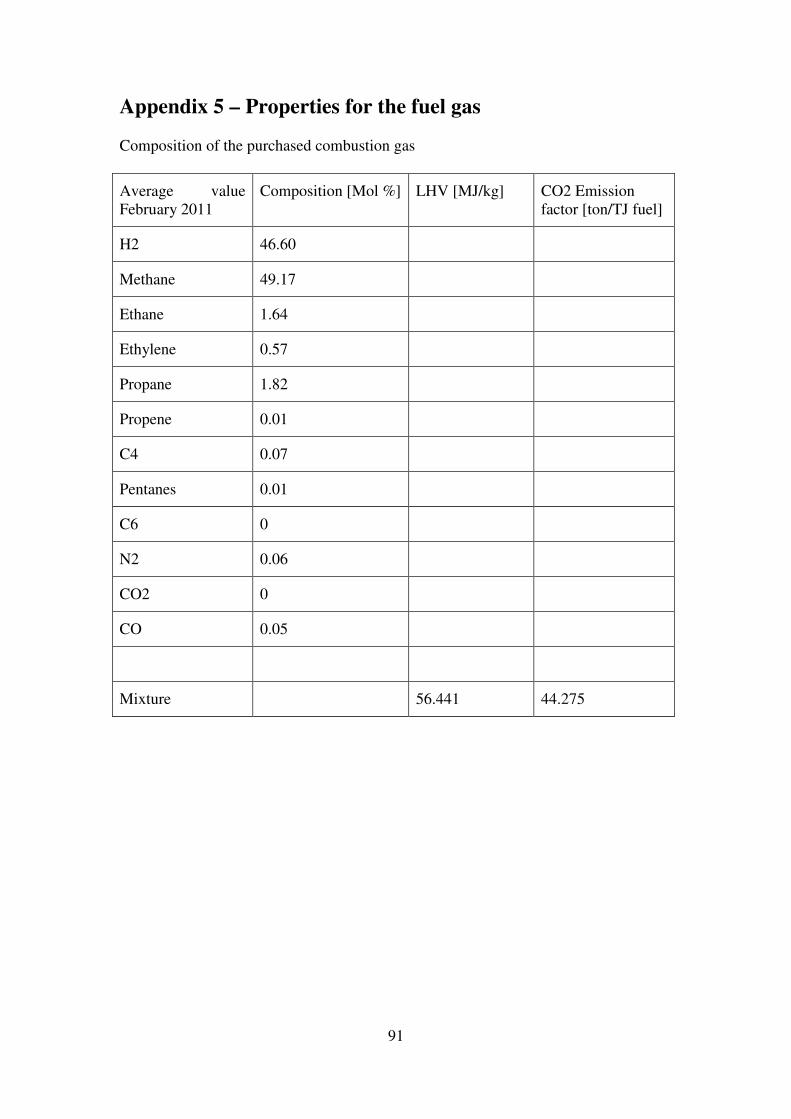
91
Appendix 5 – Properties for the fuel gas Composition of the purchased combustion gas
Average value February 2011
Composition [Mol %] LHV [MJ/kg] CO2 Emission factor [ton/TJ fuel]
H2 46.60
Methane 49.17
Ethane 1.64
Ethylene 0.57
Propane 1.82
Propene 0.01
C4 0.07
Pentanes 0.01
C6 0
N2 0.06
CO2 0
CO 0.05
Mixture 56.441 44.275

92
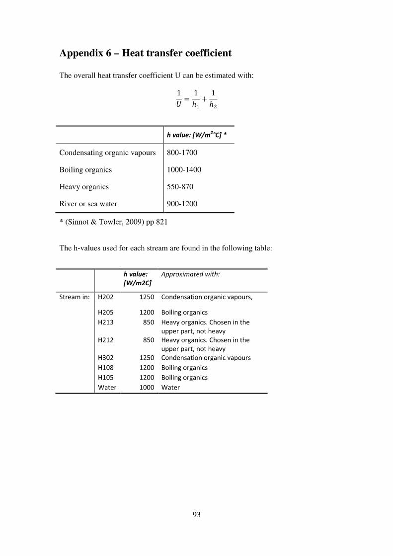
93
Appendix 6 – Heat transfer coefficient
The overall heat transfer coefficient U can be estimated with: 1
� + 1§n m 1
§�
h value: [W/m2°C] *
Condensating organic vapours 800-1700
Boiling organics 1000-1400
Heavy organics 550-870
River or sea water 900-1200
* (Sinnot & Towler, 2009) pp 821
The h-values used for each stream are found in the following table:
h value:
[W/m2C]
Approximated with:
Stream in: H202 1250 Condensation organic vapours,
H205 1200 Boiling organics
H213 850 Heavy organics. Chosen in the
upper part, not heavy
H212 850 Heavy organics. Chosen in the
upper part, not heavy
H302 1250 Condensation organic vapours
H108 1200 Boiling organics
H105 1200 Boiling organics
Water 1000 Water

94

95
Appendix 7 – Current load of the heat exchangers
In this appendix, the heat loads for the heat exchangers in the current VCM plant are found. The load is divided into two or more temperature intervals in the case of evaporation or condensation, where the difference in capacity rate could be high. Present situation. Results from Aspen simulations, put into pinch analysis Unit At: Description Tstart
[C] Ttarget [C]
Q [kW] Utility
685-03 EDC Reboiler EtCl-column 1 63.8 65 66 10 bar steam
685-04 EDC Condenser EtCl column1 62.9 59.1 60 Cooling water
685-05 EDC Reboiler EtCl-column 2 58.8 59 19 10 bar steam
685-06 EDC Condenser EtCl-column 2 52.9 32.8 19 Cooling water
H104 EDC Reboiler Tri-column EDC 133.6 145.6 74 10 bar steam
H105 EDC Reboiler Azeo column 127.7 128.5 3858 10 bar steam
H106 EDC Condenser Azeo column 85.6 30 2296 Cooling water
H106a EDC Condenser Azeo column, cooling 85.6 80.7 26
H106b EDC Condenser Azeo column, condensation 80.7 60.6 1994
H106c EDC Condenser Azeo column, cooling 60.6 30 276
H107 EDC Tar condenser (Condenser Tri-column EDC)
87.9 86.5 80 Cooling water
H108 EDC Reboiler EDC-column 111 119.1 5803 10 bar steam
H108a EDC Reboiler EDC column , cond1 111 113.75 3397
H108b EDC Reboiler EDC column , cond2 113.75 119.1 2406
H109 EDC Condenser EDC-column 89.3 35 6634 Cooling water
H109a EDC Condenser EDC-column, condensation 89.3 89.2 5413,8
H109b EDC Condenser EDC-column, cooling 89.2 35 1220
S104 EDC EDC tar boiler 140 141 78 10 bar steam
H153 HTC HTC-condenser 82.4 74.4 9482 Cooling water
H153a HTC HTC-condenser, condensation part 1 82.4 81.5 8404
H153b HTC HTC-condenser, condensation part 2 81.5 74.4 1078
H154 HTC EDC-condenser 73.5 15.8 150 Cooling water
H154a HTC EDC-condenser, condensation part 1 73.5 57.5 98,5
H154b HTC EDC-condenser, condensation part 2 57.5 15.8 51,5
H155 HTC Remaining gas condenser 15.8 -16.5 5 Propene
H158AB HTC Reboiler Tri-column HTC 118 123.5 170 10 bar steam
H159 HTC Condenser Tri-column HTC 87.1 13.9 157 Cooling water
H159a HTC Condenser Tri-column HTC, condensation
87.1 86.4 121
H159b HTC Condenser Tri-column HTC, cooling 86.4 13.9 36
H160 HTC Pure EDC-cooler 89.2 26.7 364 Cooling water
H166 HTC Cooler 57.5 34 33 Cooling water
H301 OXI HCl heater 22 179.6 342 10 bar steam
H302 OXI Precooler 217.2 93.9 2618 Cooling water
H302a OXI Precooler, condensation part 1 217.2 150 1082
H302b OXI Precooler, condensation part 2 150 93.9 1536
H303AB OXI Condenser after precooler H302 after R303
93.9 30 1641 Cooling water
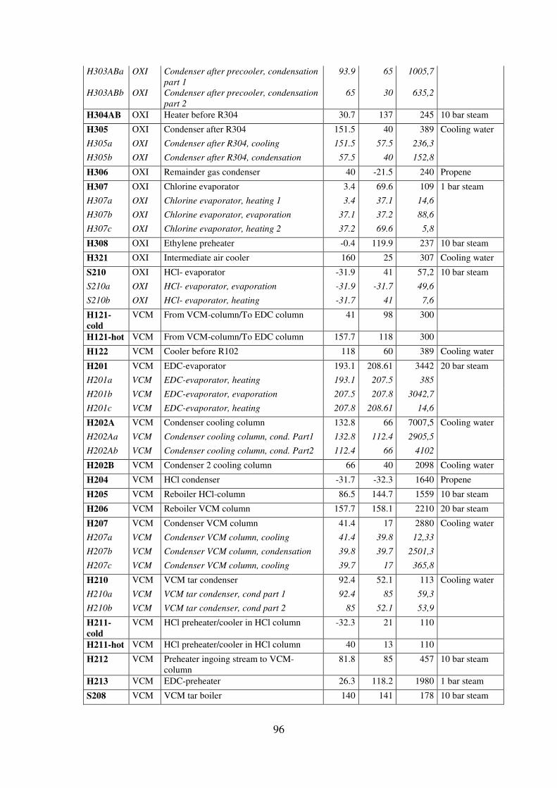
96
H303ABa OXI Condenser after precooler, condensation part 1
93.9 65 1005,7
H303ABb OXI Condenser after precooler, condensation part 2
65 30 635,2
H304AB OXI Heater before R304 30.7 137 245 10 bar steam
H305 OXI Condenser after R304 151.5 40 389 Cooling water
H305a OXI Condenser after R304, cooling 151.5 57.5 236,3
H305b OXI Condenser after R304, condensation 57.5 40 152,8
H306 OXI Remainder gas condenser 40 -21.5 240 Propene
H307 OXI Chlorine evaporator 3.4 69.6 109 1 bar steam
H307a OXI Chlorine evaporator, heating 1 3.4 37.1 14,6
H307b OXI Chlorine evaporator, evaporation 37.1 37.2 88,6
H307c OXI Chlorine evaporator, heating 2 37.2 69.6 5,8
H308 OXI Ethylene preheater -0.4 119.9 237 10 bar steam
H321 OXI Intermediate air cooler 160 25 307 Cooling water
S210 OXI HCl- evaporator -31.9 41 57,2 10 bar steam
S210a OXI HCl- evaporator, evaporation -31.9 -31.7 49,6
S210b OXI HCl- evaporator, heating -31.7 41 7,6
H121-
cold
VCM From VCM-column/To EDC column 41 98 300
H121-hot VCM From VCM-column/To EDC column 157.7 118 300
H122 VCM Cooler before R102 118 60 389 Cooling water
H201 VCM EDC-evaporator 193.1 208.61 3442 20 bar steam
H201a VCM EDC-evaporator, heating 193.1 207.5 385
H201b VCM EDC-evaporator, evaporation 207.5 207.8 3042,7
H201c VCM EDC-evaporator, heating 207.8 208.61 14,6
H202A VCM Condenser cooling column 132.8 66 7007,5 Cooling water
H202Aa VCM Condenser cooling column, cond. Part1 132.8 112.4 2905,5
H202Ab VCM Condenser cooling column, cond. Part2 112.4 66 4102
H202B VCM Condenser 2 cooling column 66 40 2098 Cooling water
H204 VCM HCl condenser -31.7 -32.3 1640 Propene
H205 VCM Reboiler HCl-column 86.5 144.7 1559 10 bar steam
H206 VCM Reboiler VCM column 157.7 158.1 2210 20 bar steam
H207 VCM Condenser VCM column 41.4 17 2880 Cooling water
H207a VCM Condenser VCM column, cooling 41.4 39.8 12,33
H207b VCM Condenser VCM column, condensation 39.8 39.7 2501,3
H207c VCM Condenser VCM column, cooling 39.7 17 365,8
H210 VCM VCM tar condenser 92.4 52.1 113 Cooling water
H210a VCM VCM tar condenser, cond part 1 92.4 85 59,3
H210b VCM VCM tar condenser, cond part 2 85 52.1 53,9
H211-
cold
VCM HCl preheater/cooler in HCl column -32.3 21 110
H211-hot VCM HCl preheater/cooler in HCl column 40 13 110
H212 VCM Preheater ingoing stream to VCM-column
81.8 85 457 10 bar steam
H213 VCM EDC-preheater 26.3 118.2 1980 1 bar steam
S208 VCM VCM tar boiler 140 141 178 10 bar steam
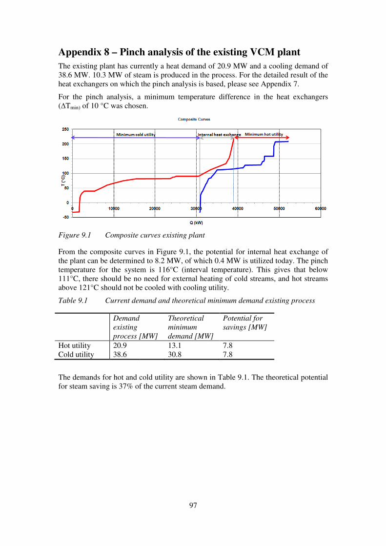
Appendix 8 – Pinch analysis of the existing VCM plant
The existing plant has currently38.6 MW. 10.3 MW of steam is produced in the process. For the detailed result of the heat exchangers on which the pinch analysis is based, please see
For the pinch analysis, a minimum temperature difference in the(∆Tmin) of 10 °C was chosen.
Figure 9.1 Composite curves existing plant
From the composite curves in the plant can be determined to 8.2 MW, of which 0.4 MW is utilized today.temperature for the system is 116°C (interval temperature). This gives that below 111°C, there should be no need for external heating of cold streams, and hot streams above 121°C should not be cooled with cooling utility.
Table 9.1 Current demand and theoretical minimum demand existing process
Demand existing process [MW]
Hot utility 20.9 Cold utility 38.6
The demands for hot and cold utility are shown in for steam saving is 37% of the current steam demand.
97
Pinch analysis of the existing VCM plant
currently a heat demand of 20.9 MW and a cooling demand of steam is produced in the process. For the detailed result of the
heat exchangers on which the pinch analysis is based, please see Appendix
For the pinch analysis, a minimum temperature difference in the heat exchangers of 10 °C was chosen.
Composite curves existing plant
From the composite curves in Figure 9.1, the potential for internal heat exchange of lant can be determined to 8.2 MW, of which 0.4 MW is utilized today.
temperature for the system is 116°C (interval temperature). This gives that below 111°C, there should be no need for external heating of cold streams, and hot streams
C should not be cooled with cooling utility.
Current demand and theoretical minimum demand existing process
Demand
process [MW]
Theoretical minimum demand [MW]
Potential for savings [MW]
13.1 7.8 30.8 7.8
The demands for hot and cold utility are shown in Table 9.1. The theoretical potential for steam saving is 37% of the current steam demand.
Pinch analysis of the existing VCM plant
0.9 MW and a cooling demand of steam is produced in the process. For the detailed result of the
Appendix 7.
heat exchangers
, the potential for internal heat exchange of lant can be determined to 8.2 MW, of which 0.4 MW is utilized today. The pinch
temperature for the system is 116°C (interval temperature). This gives that below 111°C, there should be no need for external heating of cold streams, and hot streams
Current demand and theoretical minimum demand existing process
. The theoretical potential

Figure 9.2 Grand composite curve existing plant
As seen in Figure 9.1 there is a large surplus of heat below the pinch temperature.
98
Grand composite curve existing plant
here is a large surplus of heat below the pinch temperature.
here is a large surplus of heat below the pinch temperature.

99
Appendix 9 – Future load of the heat exchangers In this appendix, the heat loads for the heat exchangers in the future VCM plant are found. The load is divided into two or more temperature intervals in the case of evaporation or condensation, where the difference in capacity rate could be high. Future situation. Results from Aspen simulations, put into pinch analysis
Unit At: Description Tstart [C]
Ttarget [C] Q [kW] Utility
685-03 EDC Reboiler EtCl-column 1 63.8 65 66 10 bar steam
685-04 EDC Condenser EtCl column1 62.9 59.1 60 Cooling water
685-05 EDC Reboiler EtCl-column 2 58.8 59 19 10 bar steam
685-06 EDC Condenser EtCl-column 2 52.9 32.8 19 Cooling water
H104 EDC Reboiler Tri-column EDC 133.6 145.6 74 10 bar steam
H105 EDC Reboiler Azeo column 127.7 128.5 3858 10 bar steam
H106 EDC Condenser Azeo column 85.6 30 2296 Cooling water
H106a EDC Condenser Azeo column, cooling 85.6 80.7 26
H106b EDC Condenser Azeo column, condensation 80.7 60.6 1994
H106c EDC Condenser Azeo column, cooling 60.6 30 276
H107 EDC Tar condenser (Condenser Tri-column) 87.9 86.5 80 Cooling water
H108 EDC Reboiler EDC-column 111 119.1 5803 10 bar steam
H108a EDC Reboiler EDC column , cond1 111 113.75 3397
H108b EDC Reboiler EDC column , cond2 113.75 119.1 2406
H109 EDC Condenser EDC-column 89.3 35 6634 Cooling water
H109a EDC Condenser EDC-column, condensation 89.3 89.2 5413,8
H109b EDC Condenser EDC-column, cooling 89.2 35 1220
S104 EDC EDC tar boiler 140 141 78 10 bar steam
H153 HTC HTC-condenser 82.4 74.4 13065 Cooling water
H153a HTC HTC-condenser, condensation part 1 82.4 81.5 11105
H153b HTC HTC-condenser, condensation part 2 81.5 74.4 1960
H154 HTC EDC-condenser 73.5 15.8 300 Cooling water
H154a HTC EDC-condenser, condensation part 1 73.5 57.5 197
H154b HTC EDC-condenser, condensation part 2 57.5 15.8 103
H155 HTC Remaining gas condenser 15.8 -16.5 10 Propene
H166 HTC Cooler 57.5 34 65 Cooling water
H160 HTC Pure EDC-cooler 89.2 26.7 1011 Cooling water
H159 HTC Condenser Tri-column HTC 87.1 13.9 104 Cooling water
H159a HTC Condenser Tri-column HTC, cond. 87.1 86.4 81
H159b HTC Condenser Tri-column HTC, cooling 86.4 13.9 23
H158AB HTC Reboiler Tri-column HTC 118 123.5 114 10 bar steam
H165 HTC Cooler R151 115 40 1600 Cooling water
H164 HTC Cooler HTC-column 100 40 1200 Cooling water
Hnew HTC New cooler HTC 100 40 3099 Cooling water
H301 OXI HCl heater 22 179.6 342 10 bar steam
H302 OXI Precooler 217.2 93.9 2618 Cooling water
H302a OXI Precooler, condensation part 1 217.2 150 1082

100
H302b OXI Precooler, condensation part 2 150 93.9 1536
H303AB OXI Condenser after precooler H302 after R303
93.9 30 1641 Cooling water
H303ABa OXI Condenser after precooler, cond. part 1 93.9 65 1005,7
H303ABb OXI Condenser after precooler, cond. part 2 65 30 635,2
H304AB OXI Heater before R304 30.7 137 245 10 bar steam
H305 OXI Condenser after R304 151.5 40 389 Cooling water
H305a OXI Condenser after R304, cooling 151.5 57.5 236,3
H305b OXI Condenser after R304, condensation 57.5 40 152,8
H306 OXI Remainder gas condenser 40 -21.5 240 Propene
H307 OXI Chlorine evaporator 3.4 69.6 109 1 bar steam
H307a OXI Chlorine evaporator, heating 1 3.4 37.1 14,6
H307b OXI Chlorine evaporator, evaporation 37.1 37.2 88,6
H307c OXI Chlorine evaporator, heating 2 37.2 69.6 5,8
H308 OXI Ethylene preheater -0.4 119.9 237 10 bar steam
H321 OXI Intermediate air cooler 160 25 307 Cooling water
S210 OXI HCl- evaporator -31.9 41 57,2 10 bar steam
S210a OXI HCl- evaporator, evaporation -31.9 -31.7 49,6
S210b OXI HCl- evaporator, heating -31.7 41 7,6
H121-cold VCM From VCM-column/To EDC column 41 98 300
H121-hot VCM From VCM-column/To EDC column 157.7 118 300
H122 VCM Cooler before R102 118 60 389 Cooling water
H201 VCM EDC-evaporator 193.1 208.61 3442 20 bar steam
H201a VCM EDC-evaporator, heating 193.1 207.5 385
H201b VCM EDC-evaporator, evaporation 207.5 207.8 3042,7
H201c VCM EDC-evaporator, heating 207.8 208.61 14,6
H202A VCM Condenser cooling column 132.8 66 7007,5 Cooling water
H202Aa VCM Condenser cooling column, cond. Part1 132.8 112.4 2905,5
H202Ab VCM Condenser cooling column, cond. Part2 112.4 66 4102
H202B VCM Condenser 2 cooling column 66 40 2098 Cooling water
H204 VCM HCl condenser -31.7 -32.3 1640 Propene
H205 VCM Reboiler HCl-column 86.5 144.7 1559 10 bar steam
H206 VCM Reboiler VCM column 157.7 158.1 2210 20 bar steam
H207 VCM Condenser VCM column 41.4 17 2880 Cooling water
H207a VCM Condenser VCM column, cooling 41.4 39.8 12,33
H207b VCM Condenser VCM column, condensation 39.8 39.7 2501,3
H207c VCM Condenser VCM column, cooling 39.7 17 365,8
H210 VCM VCM tar condenser 92.4 52.1 113 Cooling water
H210a VCM VCM tar condenser, cond part 1 92.4 85 59,3
H210b VCM VCM tar condenser, cond part 2 85 52.1 53,9
H211-cold VCM HCl preheater/cooler in HCl column -32.3 21 110
H211-hot VCM HCl preheater/cooler in HCl column 40 13 110
H212 VCM Preheater ingoing stream to VCM-column 81.8 85 457 10 bar steam
H213 VCM EDC-preheater 26.3 118.2 1980 1 bar steam
S208 VCM VCM tar boiler 140 141 178 10 bar steam
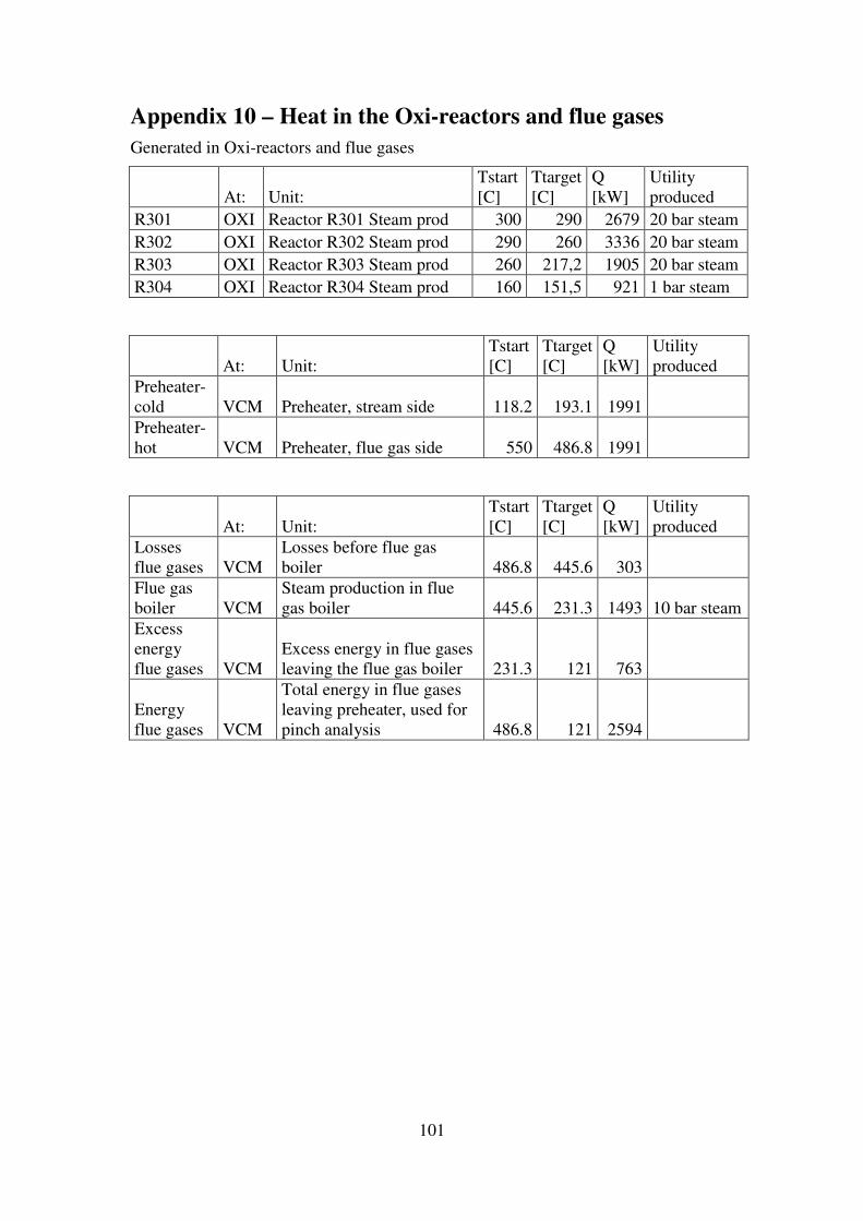
101
Appendix 10 – Heat in the Oxi-reactors and flue gases
Generated in Oxi-reactors and flue gases
At: Unit: Tstart [C]
Ttarget [C]
Q [kW]
Utility produced
R301 OXI Reactor R301 Steam prod 300 290 2679 20 bar steam R302 OXI Reactor R302 Steam prod 290 260 3336 20 bar steam R303 OXI Reactor R303 Steam prod 260 217,2 1905 20 bar steam R304 OXI Reactor R304 Steam prod 160 151,5 921 1 bar steam
At: Unit: Tstart [C]
Ttarget [C]
Q [kW]
Utility produced
Preheater-cold VCM Preheater, stream side 118.2 193.1 1991 Preheater-hot VCM Preheater, flue gas side 550 486.8 1991
At: Unit: Tstart [C]
Ttarget [C]
Q [kW]
Utility produced
Losses flue gases VCM
Losses before flue gas boiler 486.8 445.6 303
Flue gas boiler VCM
Steam production in flue gas boiler 445.6 231.3 1493 10 bar steam
Excess energy flue gases VCM
Excess energy in flue gases leaving the flue gas boiler 231.3 121 763
Energy flue gases VCM
Total energy in flue gases leaving preheater, used for pinch analysis 486.8 121 2594

102
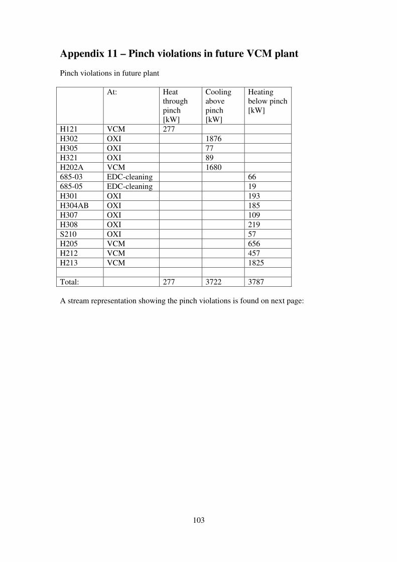
103
Appendix 11 – Pinch violations in future VCM plant Pinch violations in future plant At: Heat
through pinch [kW]
Cooling above pinch [kW]
Heating below pinch [kW]
H121 VCM 277 H302 OXI 1876 H305 OXI 77 H321 OXI 89 H202A VCM 1680 685-03 EDC-cleaning 66 685-05 EDC-cleaning 19 H301 OXI 193 H304AB OXI 185 H307 OXI 109 H308 OXI 219 S210 OXI 57 H205 VCM 656 H212 VCM 457 H213 VCM 1825 Total: 277 3722 3787 A stream representation showing the pinch violations is found on next page:

104
Future production with existing net and additional coolers
Pinch violations

105
Appendix 12 – MER network future VCM plant
A stream representation of a Maximum Energy Recovery (MER) network for the future VCM plant is found below. Note that one stream, H108, is splitted into three.
MER network future VCM plant
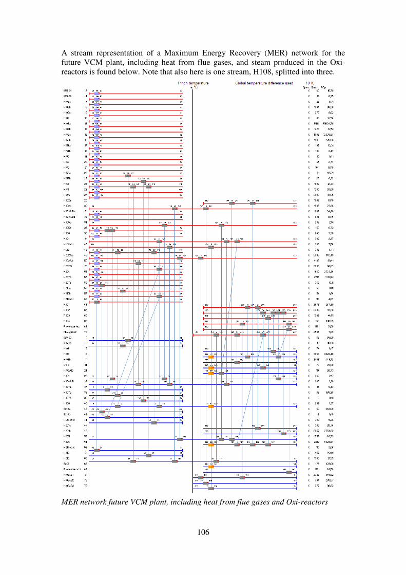
106
A stream representation of a Maximum Energy Recovery (MER) network for the future VCM plant, including heat from flue gases, and steam produced in the Oxi-reactors is found below. Note that also here is one stream, H108, splitted into three.
MER network future VCM plant, including heat from flue gases and Oxi-reactors

107
Appendix 13 – Economic evaluation of the retrofits The calculations are made following the calculation procedure described in Chapter 3.5
Q
[kW]
dTlm
[C]
U
[W/
m2K]
A
[m2]
Cost of
equipment
(Ce)
Carbon
Steel [$]
Jan 2007
Ce,
Carbon
Steel [$]
Nov
2010
Material
cost
factor
fm
ISBL
cost
C [$]
Total
fixed
capital
cost
CFC [$]
Total
fixed
capital
cost
CFC
[MSEK]
Annual
steam
savings
[GJ]
Approx.
annual
savings
[MSEK]:
Payback
period
[years]
Retrofit
1
H202 -
H205 972 21 612 75 32117 35078 1.65 153293 278993 2 29477 3.31 0.58
H202-
H213 1933 35 506 108 36696 40080 1.65 175151 318774 2 58621 6.58 0,33
H202-
H212 457 26 506 35 27251 29764 1.65 130068 236724 2 13859 1.56 1,05
Sum subsystem 1 6 101957 11.45 0.50
H302-
H108 1876 40 612 76 32357 35340 1.7 157618 286865 2 56892 6.39 0,31
Sum subsystem 2 2 56892 6.39 0.31
Sum retrofit 1: 8 158850 17.84 0.43
Retrofit
2
H202-
H108 1680 15 612 185 48187 52631 1.65 229996 418593 3 50948 5.72 0,51
H202 -
H205 656 18 612 60 30265 33056 1.65 144453 262904 2 19894 2.23 0,81
H202-
H213 1717 32 506 107 36543 39913 1.65 174419 317443 2 52070 5.85 0,38
H202-
H212 457 13 506 70 31482 34385 1.65 150263 273479 2 13859 1.56 1,22
H302-
H108 1839 40 612 75 32224 35195 1.7 156971 285686 2 55770 6.26 0,32
Sum retrofit 2: 11 192542 21.63 0.50
Retrofit
3
H202-
H108 1680 15 612 185 48187 52631 1.65 229996 418593 3 50948 5.72 0,51
H202-
H213 1825 34 506 107 36553 39924 1.65 174468 317531 2 55346 6.22 0,35
H202-
H212 457 19 506 46 28600 31237 1.65 136505 248438 2 13859 1.56 1,10
H302-
H105 973 54 612 30 26692 29153 1.7 130024 236644 2 29508 3.31 0,49
H302-
H205 1559 11 612 232 55742 60882 1.7 271533 494191 3 47279 5.31 0,64
Sum retrofit 3: 12 196940 22,12 0.54

108
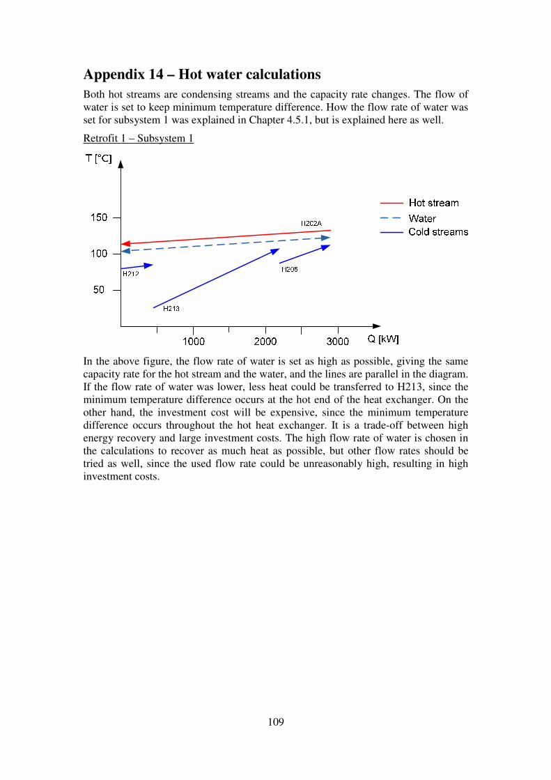
109
Appendix 14 – Hot water calculations
Both hot streams are condensing streams and the capacity rate changes. The flow of water is set to keep minimum temperature difference. How the flow rate of water was set for subsystem 1 was explained in Chapter 4.5.1, but is explained here as well.
Retrofit 1 – Subsystem 1
In the above figure, the flow rate of water is set as high as possible, giving the same capacity rate for the hot stream and the water, and the lines are parallel in the diagram. If the flow rate of water was lower, less heat could be transferred to H213, since the minimum temperature difference occurs at the hot end of the heat exchanger. On the other hand, the investment cost will be expensive, since the minimum temperature difference occurs throughout the hot heat exchanger. It is a trade-off between high energy recovery and large investment costs. The high flow rate of water is chosen in the calculations to recover as much heat as possible, but other flow rates should be tried as well, since the used flow rate could be unreasonably high, resulting in high investment costs.
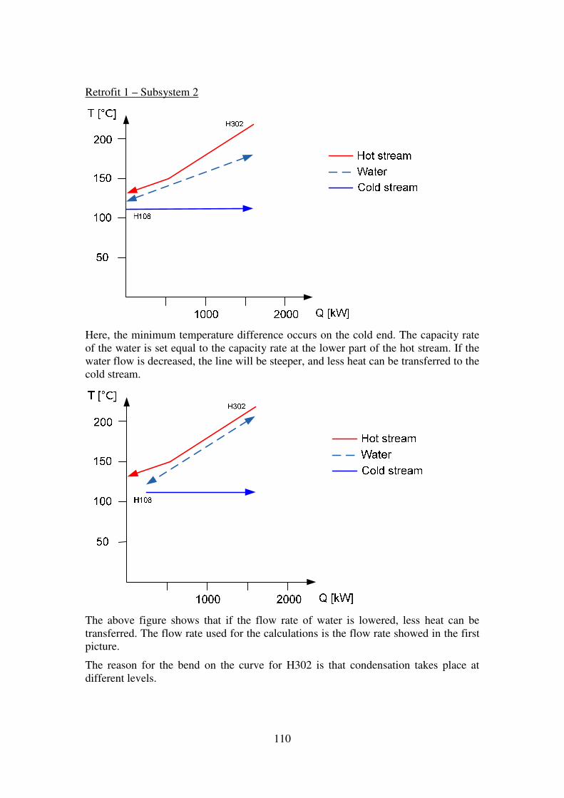
110
Retrofit 1 – Subsystem 2
Here, the minimum temperature difference occurs on the cold end. The capacity rate of the water is set equal to the capacity rate at the lower part of the hot stream. If the water flow is decreased, the line will be steeper, and less heat can be transferred to the cold stream.
The above figure shows that if the flow rate of water is lowered, less heat can be transferred. The flow rate used for the calculations is the flow rate showed in the first picture.
The reason for the bend on the curve for H302 is that condensation takes place at different levels.
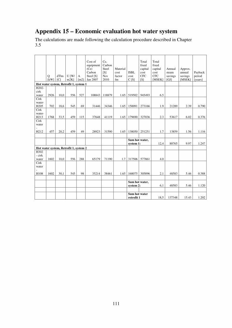
111
Appendix 15 – Economic evaluation hot water system
The calculations are made following the calculation procedure described in Chapter 3.5
Q [kW]
dTlm [C]
U [W/ m2K]
A [m2]
Cost of equipment (Ce) Carbon Steel [$] Jan 2007
Ce, Carbon Steel [$] Nov 2010
Material cost factor fm
ISBL cost C [$]
Total fixed capital cost CFC [$]
Total fixed capital cost CFC [MSEK]
Annual steam savings [GJ]
Approx. annual savings [MSEK]
Payback period [years]
Hot water system, Retrofit 1, system 1 H202-cirk water 2926 10,0 556 527 108843 118879 1.65 519502 945493 6.5 Cirk water-H205 702 18,6 545 69 31446 34346 1.65 150091 273166 1.9 21289 2.39 0.790 Cirk water-H213 1768 33,5 459 115 37648 41119 1.65 179690 327036 2.3 53617 6.02 0.376 Cirk water - H212 457 20,2 459 49 28923 31590 1.65 138050 251251 1.7 13859 1.56 1.116
Sum hot water,
system 1: 12,4 88765 9.97 1.247
Hot water system, Retrofit 1, system 2 H302 - cirk water 1602 10,0 556 288 65179 71190 1.7 317506 577861 4.0 Cirk water - H108 1602 30,1 545 98 35214 38461 1.65 168075 305896 2.1 48583 5.46 0.388
Sum hot water,
system 2: 6,1 48583 5.46 1.120
Sum hot water
retrofit 1 18,5 137348 15.43 1.202

112
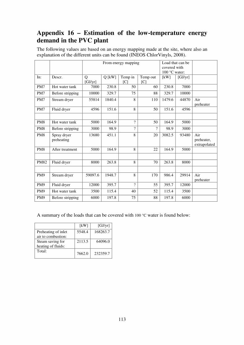
113
Appendix 16 – Estimation of the low-temperature energy
demand in the PVC plant
The following values are based on an energy mapping made at the site, where also an explanation of the different units can be found (INEOS ChlorVinyls, 2008).
From energy mapping Load that can be covered with 100 °C water:
In: Descr. Q [GJ/yr]
Q [kW] Temp in [C]
Temp out [C]
[kW] [GJ/yr]
PM7 Hot water tank 7000 230.8 50 60 230.8 7000
PM7 Before stripping 10000 329.7 75 88 329.7 10000
PM7 Stream dryer 55814 1840.4 8 110 1479.6 44870 Air preheater
PM7 Fluid dryer 4596 151.6 8 50 151.6 4596
PM8 Hot water tank 5000 164.9 ? 50 164.9 5000
PM8 Before stripping 3000 98.9 ? ? 98.9 3000
PM8 Spray dryer preheating
13680 451.1 8 20 3082.5 93480 Air preheater, extrapolated
PM8 After treatment 5000 164.9 8 22 164.9 5000
PM82 Fluid dryer 8000 263.8 8 70 263.8 8000
PM9 Stream dryer 59097.6 1948.7 8 170 986.4 29914 Air preheater
PM9 Fluid dryer 12000 395.7 ? 55 395.7 12000
PM9 Hot water tank 3500 115.4 40 52 115.4 3500
PM9 Before stripping 6000 197.8 75 88 197.8 6000
A summary of the loads that can be covered with 100 °C water is found below:
[kW] [GJ/yr]
Preheating of inlet air to combustion:
5548.4 168263.7
Steam saving for heating of fluids:
2113.5 64096.0
Total: 7662.0 232359.7

114
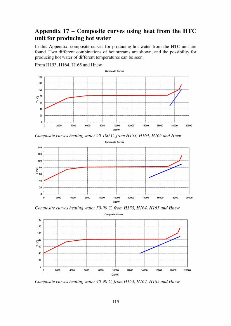
115
Appendix 17 – Composite curves using heat from the HTC
unit for producing hot water
In this Appendix, composite curves for producing hot water from the HTC-unit are found. Two different combinations of hot streams are shown, and the possibility for producing hot water of different temperatures can be seen.
From H153, H164, H165 and Hnew
Composite curves heating water 50-100 C, from H153, H164, H165 and Hnew
Composite curves heating water 50-90 C, from H153, H164, H165 and Hnew
Composite curves heating water 40-90 C, from H153, H164, H165 and Hnew
0
20
40
60
80
100
120
140
0 2000 4000 6000 8000 10000 12000 14000 16000 18000 20000
T (°C
)
Q (kW)
Composite Curves
0
20
40
60
80
100
120
140
0 2000 4000 6000 8000 10000 12000 14000 16000 18000 20000
T (°C
)
Q (kW)
Composite Curves
0
20
40
60
80
100
120
140
0 2000 4000 6000 8000 10000 12000 14000 16000 18000 20000
T (°C
)
Q (kW)
Composite Curves
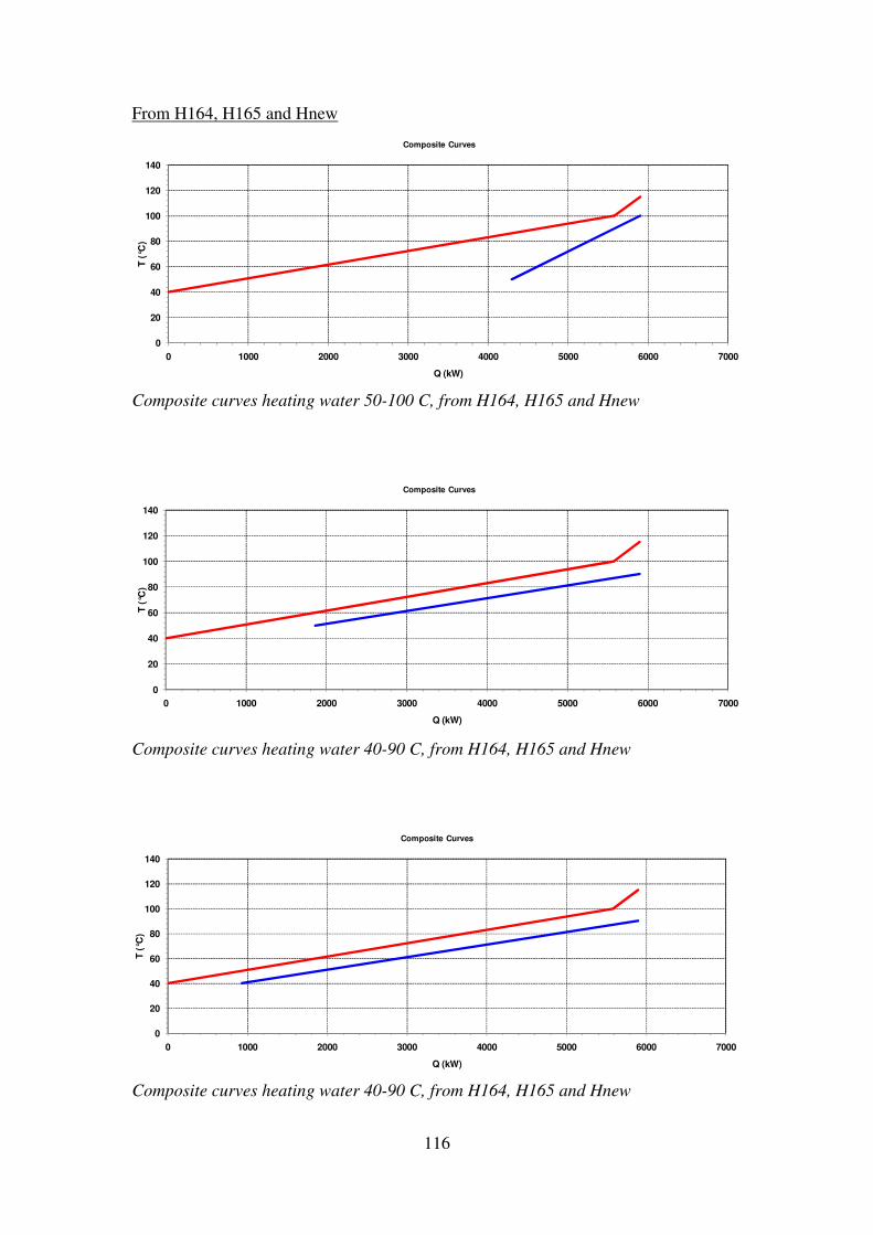
116
From H164, H165 and Hnew
Composite curves heating water 50-100 C, from H164, H165 and Hnew
Composite curves heating water 40-90 C, from H164, H165 and Hnew
Composite curves heating water 40-90 C, from H164, H165 and Hnew
0
20
40
60
80
100
120
140
0 1000 2000 3000 4000 5000 6000 7000
T (°C
)
Q (kW)
Composite Curves
0
20
40
60
80
100
120
140
0 1000 2000 3000 4000 5000 6000 7000
T (°C
)
Q (kW)
Composite Curves
0
20
40
60
80
100
120
140
0 1000 2000 3000 4000 5000 6000 7000
T (°C
)
Q (kW)
Composite Curves
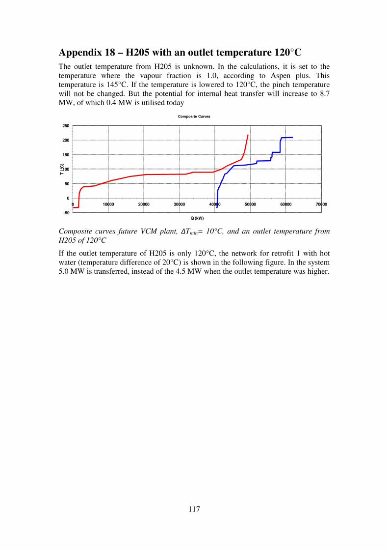
117
Appendix 18 – H205 with an outlet temperature 120°C
The outlet temperature from H205 is unknown. In the calculations, it is set to the temperature where the vapour fraction is 1.0, according to Aspen plus. This temperature is 145°C. If the temperature is lowered to 120°C, the pinch temperature will not be changed. But the potential for internal heat transfer will increase to 8.7 MW, of which 0.4 MW is utilised today
Composite curves future VCM plant, ΔTmin= 10°C, and an outlet temperature from H205 of 120°C
If the outlet temperature of H205 is only 120°C, the network for retrofit 1 with hot water (temperature difference of 20°C) is shown in the following figure. In the system 5.0 MW is transferred, instead of the 4.5 MW when the outlet temperature was higher.
-50
0
50
100
150
200
250
0 10000 20000 30000 40000 50000 60000 70000
T (°C
)
Q (kW)
Composite Curves

118
Stream representation for retrofit 1 with hot water system, ΔTmin= 20°C, and an outlet temperature from H205 of 120°C