Proceedings of the 5th International Conference on Inverse Problems in Engineering: Theory and Practice, Cambridge, UK, 11-15th July 2005 IDENTIFICATION OF DIFFUSION COEFFICIENTS DURING POST-DISCHARGE NITRIDING J. BERNAL-PONCE1, A. FRAGUELA-COLLAR2, J. A. GÓMEZ3, J. OSEGUERA-PEÑA4 and F. CASTILLO-ARANGUREN4

1Departamento de Ingeniería Mecánica, ITESM-Toluca, México, jbernal@itesm.mx2Facultad de Ciencias Físico-Matemáticas, BUAP, México, fraguela@fismat.buap.mx3Departamento de Ingeniería Matemática, UFRO, Chile, jagomez@ufro.cl4División de Ingeniería y Arquitectura, ITESM-CEM, México, joseguer@itesm.mx, francast@itesm.mx Abstract- This work presents a model for computing the diffusion coefficients during post-discharge nitriding through an inverse problem of coefficient identification in a diffusion model, which considers several layers and Stefan type conditions. An approximate solution corresponding to a quasi-stationary state is obtained for the model, using qualitative and quantitative information from experimental results. To study the inverse problem we assume that we have information about the nitrogen concentration at different depths in the solid after the stabilization of the layers in the post-discharge nitriding process. To develop a numerical algorithm for the identification of the diffusion coefficients, a functional to be minimized is built. This functional measures the deviation between the data theoretically obtained from the approximate solution of the model and the experimental data. 1. INTRODUCTION

Thermo-chemical nitriding treatment produces an important improvement in the mechanical, tribological and chemical properties in steel, thus enhancing the resistance to their fatigue, corrosion and wear [1, 7, 8].

In most of the mathematical simulations of nitrogen diffusion in iron or steel reported, nitrogen concentration on the surface is taken to be constant from the beginning of the treatment [4, 5, 9,10, 11, 14, 15, 16, 18] and consequently it is considered that the thickness of the layers is zero at the initial moment. The evolution of the nitrogen concentration on the surface is inherent to the process. In processes where the diffusion takes place through a thermo-chemical balance between a gaseous mixture and the solid, i.e. mixtures with ammonia, nitrogen concentration on the surface depends on the nitrogen potential [4, 14, 16].

During weakly ionized plasma assisted processes, pulverization, adsorption and diffusion events take place on the specimen surface [10, 11]. The nitrogen concentration on the surface evolves quickly and corresponds to a dynamic balance between pulverization towards the atmosphere and the diffusion towards the solid.

Control or automation of nitriding processes depends on the means requires to identify the nitrogen concentration on the surface as well as on a mathematical model adapted to estimate the growth kinetics of compact concomitant nitride layers. On the other hand, the understanding and interpretation of the mechanisms of mass transport in solid requires experimental validation of the diffusion coefficients.

In computing diffusion coefficients, using experimental results, it has been assumed that the nitrogen concentration has a parabolic growth profile in each layer from the beginning of the process, nevertheless the nitrogen assumes different forms in each process and depends on each one. If the nitrogen concentration on the surface evolves slowly, the parabolic regime will not be observed during the initial stages, moreover the accuracy in computing diffusion coefficients will be limited [4, 5, 10, 11, 14, 16, 18].

Nitriding post-discharge processes generate an atmosphere of excited neutral or dissociated species [2, 3, 5, 12, 13]. These species produce a fast evolution of the nitrogen concentration on the surface [3].

It has been observed that the presence of atomic nitrogen in post-discharge processes significantly increases the mass transfer to a solid compared to other processes.

Based on experimental results obtained from iron nitriding, in an atmosphere produced by post-discharge microwaves, the present work considers a one-dimensional model of layer kinetic growth, and studies the inverse problem of diffusion coefficients identification in each phase from the consideration of the stabilization of the layers after a certain period of treatment. Such consideration was justified from an experimental point of view and also by taking into account the analytical expression of the layer growth kinetics.

The experimental results obtained by means of treatments assisted during post-discharge generated by a microwave source allow the accurate determination of the values of the diffusion coefficients on the basis of the solution of an inverse problem which identifies the coefficients in a one-dimensional model of kinetic growth of concomitant nitride layers.

2. EXPERIMENTAL PROCEDURE

Samples were obtained from an ARMCO iron bar (25.4 mm in diameter and 7 mm thick, Mn 880 ppm; C and P, 200 ppm; and S 150 ppm). Nitriding was carried out in a post-discharge microwave-generated plasma described elsewhere [3]. The general sequence of the nitriding experiments started with heating up the sample to 893 K in a

B05

tubular resistance furnace in a non-oxidized and non-nitriding atmosphere composed of 26Ar-80H2 sccm at a total pressure of 900 Pa. The applied and reflected were 200 W and 65 W respectively, and the distance from the discharge point was 7 cm. Upon reaching the prescribed temperature, the temperature, the atmosphere was switched to a mixture of 300N2-26Ar-80H2 at 1200 Pa and recording of the nitriding time started. After the nitriding time was completed, the atmosphere was switched back to the initial non-oxidizing, non nitriding atmosphere.

Figure 1 presents a cross-sectional view of a sample nitrided for 120 min under the conditions described previously. The nitrides below the compact nitride layer precipitated during the cooling of the sample due to the desaturation of the ferrite; the width of this zone is between 40 to 50 µ m. However, the diffusion zone of the nitrogen

in the ferrite is about 3 mm.

Figure 1. Cross sectional view of a nitrided iron sample, under post-discharge conditions. 3. MATHEMATICAL MODEL

Let us propose a mathematical model which describes the growth of the layers during the post-discharge nitriding process. We suppose that the diffusion is one-dimensional and planar and the temperature at every point in the specimen is identical during the whole process. This model presents five steps. The first step ends when the surface

reaches the equilibrium concentration at a time . This step is modeled by: SC 0t

)4(0,),(lim

)3(0,|)(),0(

)2(0,)0,(

)1(0,0,

0

0

0

2

2

>=

>−=∂∂

+∞<<=

>+∞<<∂∂

=∂∂

∞+→

=

tCtxC

tCCD

txC

xCxC

txxCD

tC

x

xeqλ

where λ is the kinetic reaction coefficient, is the diffusion coefficient, is the equilibrium nitrogen

concentration in the atmosphere remote from the surface and represents the nitrogen concentration for time

and depth

D eqC),( txC t

x . The solution of (1)-(4) is given by:

( ) ( ) ⎟⎟⎠

⎞⎜⎜⎝

⎛+⎟⎟

⎠

⎞⎜⎜⎝

⎛++⎟

⎟⎠

⎞⎜⎜⎝

⎛=

−

−2/1

2/12/10

2

2/100 2

exp2

tDDt

xerfctD

xDDt

xerfCCCC

eq

eq λλλ

where

∫∫∞+ −− =−≡≡

x

xdexerfxerfcdexerf ξ

πξ

πξξ 22 2

)(1)(,2

)(0

A certain should pass for the concentration to reach the threshold value , which follows from 0t SC

B052

( ) ⎟⎠⎞

⎜⎝⎛

⎟⎟⎠

⎞⎜⎜⎝

⎛=

−

− 2/102/10

2

0

exp tD

erfctDCC

CC

eq

eq λλ

Let us put

( ) ⎪⎭

⎪⎬⎫

⎪⎩

⎪⎨⎧

⎟⎟⎠

⎞⎜⎜⎝

⎛+⎟⎟

⎠

⎞⎜⎜⎝

⎛++⎟⎟

⎠

⎞⎜⎜⎝

⎛−

+=≡

2/102/12/1

0

0

2

2/10

0

0

)(2

exp)(2

)(

),()(

tDDt

xerfctD

xDDt

xerfCC

CtxCxf

eq

eq

λλλ

where denotes the initial concentration profile when the layer formation begins. )(xfFrom the starting profile two layers of nitrogen and a diffusion zone begin to be formed and they slowly

displace into the interior of the metal. In each layer and diffusion zone, diffusion coefficient takes a constant value

. Between adjacent layers and diffusion zone there is a jump in concentration. In each of the first two

layers a minimum constant value is reached. For every let us define

3,2,1, =iDi

2,1,min =iC i0tt > 2,1,)( =itiξ as the

depth of the corresponding layer. Since diffusion coefficients are constants, it follows that the concentration in each

layer is a decreasing function of the depth, then )(tiξ is the depth at which the concentration reaches the minimum

value (see Figures 2a-d). As a consequence of the process, there is an experimental value of the

concentration and a time such that . In this situation we say that the

layer was completely formed at time , as shown schematically in Fig. 2 b-d. We shall assume . For

2,1,min =iC i

ii CC minmax < itt = 2,1,))(( 1max == + iCtf i

iiξ

it 21 tt < ),[ 10 ttt ∈

the concentration has a jump in length . Moreover, for the length of the jump in

concentration in

2,1)),((min =− itfC ii ξ itt >

)( ii tξ is constant and equal to . In Figures 2a-d we

denote

2,1,1maxmin =− + iCC ii

2,1,)( == itx iii ξ .

…. ….

|

(a) (b)

… …. (c) (d)

C3max

C2min

C2max

C1min

t*<t0

C3min

X01 X02 Xα

Cs

C3max

C2min

C2max

C1min

X01 X02

t1

C3min

Xα X1

Cs

C3max

C2min

C2max

C1min

t2

C3min

X01 X02 Xα X2

C3max

C2min

C2max

C1min

C3min

Cs t(st)

Xγ´ Xγ Xα

Figures 2a-d. Schematic representation of nitrogen concentration as a function of depth for the case of a two compact nitride layers where nitrogen is in solution in ferrite. In what follows, we propose a model for the process of post-discharge nitriding from the starting profile . This

model describes the beginning of the layers and interfaces formation. We consider three stages:

)(xf

B053

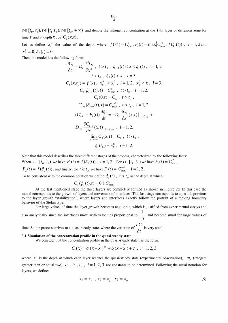
),[),,[),,[ 22110 ∞+∈∈∈ tttttttt and denote the nitrogen concentration at the -th layer or diffusion zone for

time and at depth

it x , by . ),( txCi

Let us define the value of the depth where 0ix { }))((,max)(,)( 1

maxmin0 tfCtFCxf i

ii

ii ξ+== , 2,1=i and

.0)(,0 000 ≡≡ tx ξ

Then, the model has the following form:

2,1,)()(,, 102

2

=<<>∂

∂=

∂∂

− itxtttxC

Dt

Cii

ii

i ξξ

.3,)(, 20 =<> ixttt ξ

.3,,2,1,,)(),( 02

0010 =<=<= − ixxixxxftxC iii

,2,1,,)),(( 0min0 =>=− ittCttC iii ξ

,,),0( 01 ttCtC S >=

,2,1,,)),(( 1max01 =>= +

++ ittCttC ii

ii ξ

,2,1,|),(

|),())((

0

0

11

min

=∂

∂

+∂

∂−=−

+

−

=+

+

=

itxx

CD

txx

CD

dtd

tFC

i

i

xi

i

xi

ii

ii

ξ

ξξ

,,),(lim 003 ttCtxCx

>=+∞→

.2,1,)( 00 == ixt iiξ

Note that this model describes the three different stages of the process, characterized by the following facts:

When we have ),[ 10 ttt ∈ 2,1,))(()( == itftF ii ξ . For ),[ 21 ttt ∈ we have , 2max1 )( CtF =

))(()( 22 tftF ξ= , and finally, for we have . 2tt ≥ 2,1,)( 1max == + iCtF i

i

To be consistent with the common notation we define 03 ,)( ttt >ξ as the depth at which:

3max33 1.0)),(( CttC =ξ

At the last mentioned stage the three layers are completely formed as shown in Figure 2d. In this case the model corresponds to the growth of layers and movement of interfaces. This last stage corresponds to a period, previous to the layer growth “stabilization”, where layers and interfaces exactly follow the portrait of a moving boundary behavior of the Stefan type.

For large values of time the layer growth becomes negligible, which is justified from experimental essays and

also analytically since the interfaces move with velocities proportional to t

1 and become small for large values of

time. So the process arrives to a quasi-steady state, where the variation of tC

∂∂

is very small.

3.1 Simulation of the concentration profile in the quasi-steady state We consider that the concentration profile in the quasi-steady state has the form:

3,2,1,)()()(~~

=+−+−= icxxbxxaxC iiim

iiii

where is the depth at which each layer reaches the quasi-steady state (experimental observation), (integers

greater than or equal two), are constants to be determined. Following the usual notation for

layers, we define:

ix~

im3,2,1,,, =icba iii

(5) αγγ xxxxxx === 3

~

2

~

'1

~

,,

B054

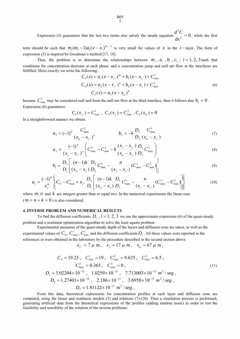
Expression (5) guarantees that the last two terms also satisfy the steady equation 02

2

=dx

Cd, while the first

term should be such that is very small for values of 2~

)()1( −−− imiiii xxamm x in the layer. The form of

expression (5) is inspired by Goodman’s method [17, 18].

−i

Thus, the problem is to determine the relationships between such that

conditions for concentration decrease at each phase, and a concentration jump and null net flow at the interfaces are fulfilled. More exactly we write the following:

3,2,1,,,, =icbam iiii

1min'1'11 )()()( CxxbxxaxC m +−+−= γγ

(6) 2min222 )()()( CxxbxxaxC n +−+−= γγ

. kxxaxC )()( 33 α−=

because may be considered null and from the null net flow at the third interface, then it follows that 3minC 03 =b .

Expression (6) guarantees:

0)(,)(,)( 32min2

1min'1 === αγγ xCCxCCxC

In a straightforward manner we obtain:

kk

xxC

a)(

)1('

3max

3γα −

−= )(

3max

2

32

γα xxC

DD

kb−

−= (7)

⎟⎟⎠

⎞⎜⎜⎝

⎛

−

−−−

−−

= 3max

2

3'2min

2max

'2 )(

)(

)(

)1( CDD

xxxx

kCCxx

a n

n

γα

γγ

γγ

(8)

⎥⎥⎦

⎤

⎢⎢⎣

⎡−

−−

−−

= )()()(

)1( 2min

2max

'

3max

2

3

1

21 CC

xxnC

DD

xxkn

DDb

γγγα

(9)

⎪⎭

⎪⎬⎫

⎪⎩

⎪⎨⎧

⎥⎥⎦

⎤

⎢⎢⎣

⎡−

−−

−−

+−−

= )()()(

)1()1( 2min

2max

'

3max

2

3

1

2'

1min

'1 CC

xxnC

DD

xxkn

DDxCC

xa Sm

m

γγγαγ

γ

(10)

where and k are integers greater than or equal two. In the numerical experiments the linear case

( ) is also considered.

nm,0=== knm

4. INVERSE PROBLEM AND NUMERICAL RESULTS

To find the diffusion coefficients 3,2,1, =iDi we use the approximate expression (6) of the quasi-steady

problem and a nonlinear optimization algorithm to solve the least square problem. Experimental measures of the quasi-steady depth of the layers and diffusion zone are taken, as well as the

experimental values of and the diffusion coefficients . All these values were reported in the

references or were obtained in the laboratory by the procedure described in the second section above.

iiS CCC minmax ,, iD

,67,17,7' mxmxmx µµµ αγγ ===

,5.6,625.9,19,25.19 2min

2max

1min ==== CCCCS

(11) ,0,365.0 3min

3max == CC

,/10713003.7,100259.1,1002204.3 21313131 segmD −−− ×××=

,/106958.3,10186.2,1027401.1 21313142 segmD −−− ×××=

,/1083122.1 2113 segmD −×=

From this data, theoretical expressions for concentration profiles at each layer and diffusion zone are computed, using the linear and nonlinear models (5) and relations (7)-(10). Then a simulation process is performed, generating artificial data from the theoretical expressions of the profiles (adding random noise) in order to test the feasibility and sensibility of the solution of the inverse problems.

B055

Due to technical difficulties in obtaining real measurements in the first two layers, the artificial data

are generated only at depths )(^

ji yC my j µ8,6,4,2= , corresponding to those layers, and at depths

Njmy j ,....,5, =µ , in the diffusion zone.

Afterwards, we use the generated data to solve the least-square problem of minimizing the function:

+⎥⎦⎤

⎢⎣⎡ −+⎥⎦

⎤⎢⎣⎡ −+⎥⎦

⎤⎢⎣⎡ −=⎟⎟

⎠

⎞⎜⎜⎝

⎛ 2^

113

2^

112

2^

1112

3

1

2 )6()6()4()4()2()2(, CCCCCCDD

DD

J ααα

∑=

⎥⎦⎤

⎢⎣⎡ −+⎥⎦

⎤⎢⎣⎡ −

N

jjj yCyCCC

5

2^

33

2^

224 )()()8()8(α

where the function represents the error between the analytical and experimental concentration data, meanwhile J

Nji ji ,...,5,,4,...,1, == αα represent different weights in which may improve the estimates of J1

2

DD

and

2

3

DD

.

Computing was performed on a PC at 900 Mhz, using MATLAB regression programs version 6.5. The results of preliminary numerical experiments for the linear model )0( === knm yield:

- Estimates of 1

2

DD

and 2

3

DD

are not sensitive to the increase of the number of measurements in the diffusion zone

when the artificial data do not have random errors.

- Estimates are very sensitive to the initial vector in the optimization process. It seems that an initial of 2

3

DD

close to the

order of the actual values is the best option, while for 1

2

DD

the initial value does not influent the result when random

errors are not considered. - Estimates are also sensitive to measurements errors.

The results of the numerical experiments for a nonlinear model )3,2( === knm , using a more robust

optimization algorithm yield: - Estimates are exacts when the artificial data do not have random errors.

- Estimates are sensitive to measurement errors, specially the quotient1

2

DD

. A regularization process is required.

- Under the presence of error measurements, the estimates are not significantly different when the data increase in the diffusion zone and large weight coefficients are included in the sum of squares . J

In the nonlinear case, several thousands of problems were solved, generating concentration data Zdata with

random perturbation of the values of given in (11). The concentration data were also perturbed with

random errors of 3 %, while random generated quotients

321 ,, DDD

1

2

DD

and 2

3

DD

were used as initial solutions for the

optimization algorithm. The following graphics, corresponding to MATLAB figures of 240 problems runs, illustrate the numerical results.

4.1 Some illustrative graphics

Figure 3 shows values of the maximal residual errors between the artificial data and the model data, given by the diffusion coefficients estimated only from four measurements in the first two layers and using weight coefficients equal to one (diamonds). These values are compared to the same difference related to diffusion coefficients estimated

from twelve measurements and weight coefficients equal to (asterisks). The residuals values are always small and there are no significant residual differences between both estimates.

610

B056

Figure 3.

Figure 4 shows the ANOVA box picture, which compares residual mean differences and exhibits the distribution of the corresponding data around the mean value.

Figure 4.

B057

Figure 5.

Figure 5 shows the ANOVA comparison interval, which exhibits no significant difference between the residual means. Only in very few cases (1% of all the numerical experiments) significant differences between those mean values were noticed.

5. CONCLUSIONS

A new approach to a free boundary model with Stefan type conditions which describes the nitriding post-discharge process is presented. Under the assumption of reaching a quasi-steady state for large times, an approximate analytical solution is proposed, which is used to recover diffusion coefficients in each layer though an optimization

algorithm. Numerical experiments show a good fitness for the data and quotient . However, a regularization

process should be considered because the quotient is always badly estimated when measurement errors are

taken into account.

23 / DD

21 / DD

REFERENCES 1. T. Bell and H. Thomas, Cyclic stressing of gas nitrocarburized low carbon steel. Metallurgical Trans. (1979) 10A,

79-85.

2. S.T. Belmonte, S. Bocke , H. Michel and D. Ablitzer, Study of transport phenomena by 3D modeling of a microwave post-discharge nitriding reactor. Surf. Coat. Technol. (1999) 112, 5-9.

3. J.L. Bernal, O. Salas, U. Figueroa and J. Oseguera, Early stages of 'γ nucleation and growth in a post-discharge

nitriding reactor. Surf. Coat. Technol. (2004) 177-178, 665-670.

4. H. Du and J. Agren, Z. Gaseous nitriding iron-evaluation of diffusion data of N in 'γ and ε phases. Metallhk.

(1995) 86, 522-529.

5. U. Figueroa, J. Oseguera and P.S. Shabes-Retchkiman, Growth kinetics of concomitant nitride layers in postdischarge conditions: modeling and experiment. Surf. Coat. Technol. (1996) 86-87, 728-734.

6. T.R. Goodman, Application of integral methods to transient nonlinear heat transfer, Advances in Heat Transfer, Academic Press, New York, 1964, pp.51-122.

B058

7. J. Grosch, J. Morral and M. Scheider, Proc. Second Conf. Carburazing and Nitriding with Atmospheres, 6-8 Dec. 1995, Cleveland, Oh, ASM International.

8. M.B. Karamis and E. Gercekcioblu, Wear behavior of plasma nitrided steels at ambient and elevated temperatures. Wear (2000) 243, 76-84.

9. S.K. Lee and H.C. Shih, Structure and corrosive wear resistance of plasma-nitrided alloy steels in 3% sodium chloride solutions. Corrosion (1994) 50, 848-853.

10. A. Marciniak, Equilibrium and non equilibrium models of layer formation during plasma and gas nitriding. Surface Eng. (1985) 1, 283-288.

11. E. Metin and O.T. Inal, Kinetics of layer growth and multiphase diffusion on ion-nitrided titanium. Metallurgical Trans. (1989) 20A, 1819-1832.

12. A. Ricard, M. Gaillard, V. Monna, A. Vesel and M. Mozetic, Excited species in H2, N2, O2, microwave flowing discharges and post-discharges. Surf. Coat. Technol. (2001) 142-144, 333-336.

13. A. Ricard, J.E. Oseguera Peña, l. Falk, H. Michel and M. Gantois, Active species in microwave post-discharge for steel surface nitriding. IEEE Trans. Plasma Sci. (1990) 18(6), 940-943.

14. K. Schwerdfteger, P. Grieveson and E.T. Turkdogan, Growth rate of Fe4Non alpha iron in NH3-H2 gas mixtures:self-diffusivity of nitrogen. Trans. Metallurgical Soc. AIME (1969) 245, 2461-2466.

15. M.A.J. Somers and Mittemeijer, Layer-growth kinetics on gaseous nitriding of pure iron: evaluation of diffusion coefficients for nitrogen in iron nitrides. Metallurgical Materials Trans. (1995) 26A, 57-74.

16. J. Torchane, P. Bilinger, J. Dulcy and M. Gantois, Control of iron nitride layers growth kinetics in the binary Fe-N system. Metallurgical Materials Trans. (1996) 27A, 1823-1835.

17. Lifang Xia and Mufu Yan, Mathematical models of nitrogen concentration profile of ion nitrided layers and computer simulation. Acta Metallurgica (1989) 2, 18-26.

18. Mufu Yan, Jihong Yan and T. Bell, Numerical simulation of nitrided layer growth and nitrogen distribution in

NFeNFe 432 ', −− − γε and a Fe−α during pulse plasma nitriding of pure iron. Modeling Simul. Mater. Sci. Eng. (2000) 8, 491-496.

B059