problems electric quadrupole moment

004 Nuclear Physk

19. C.M.G. Lattes, GP.S. Occhialini and C.F. Powell, Nature, 116, 453

(1947). 20. P. Freier, E.J. Lofgren, E.P. Ney, F. Oppenheimer, H.L.

Peters, Phys. Rev. 74, 213 (1948).

Problems

1. The radius of the solar system is 1.2 x 1013 m and the

within it is 10T*T. What is the maximum energy of the be confined within the solar system?

2 Calculate the kinetic energy of the muon emitted in the decay rest assuming m« = 139.58 MeV and «p = 105.66 MeV.

3. Calculate the maximum kinetic energy of the electrons in

aP'

4. A positron of kinetic energy 4 moc collides with an photons are emitted at equal angles (0) w.r.t. to the direction

positron. Find 0. 5 Prove that in Anderson’s experiment on the discovery of

panicle emerging from the lead plate is a proton (of ! then its kinetic energy should be 0.3 MeV. What will be its

if it is a positron ? 6 Calculate the radius of the earth in Stoermer unit for protons

energies 1,10,59.6 and 100 GeV. The magnetic dipole moment

is A# = 8.1 x 1022 J/T. Radius of the earth = 6378.16 km. 7 Show that the radiation unit of length in the electronic

theory has the values 0.52 cm and 330 m respectively m air

8. What is the percentage change in the mean life of muons

500 MeV ?

APPENDIX A-I

ELECTRIC QUADRUPOLE MOMENT

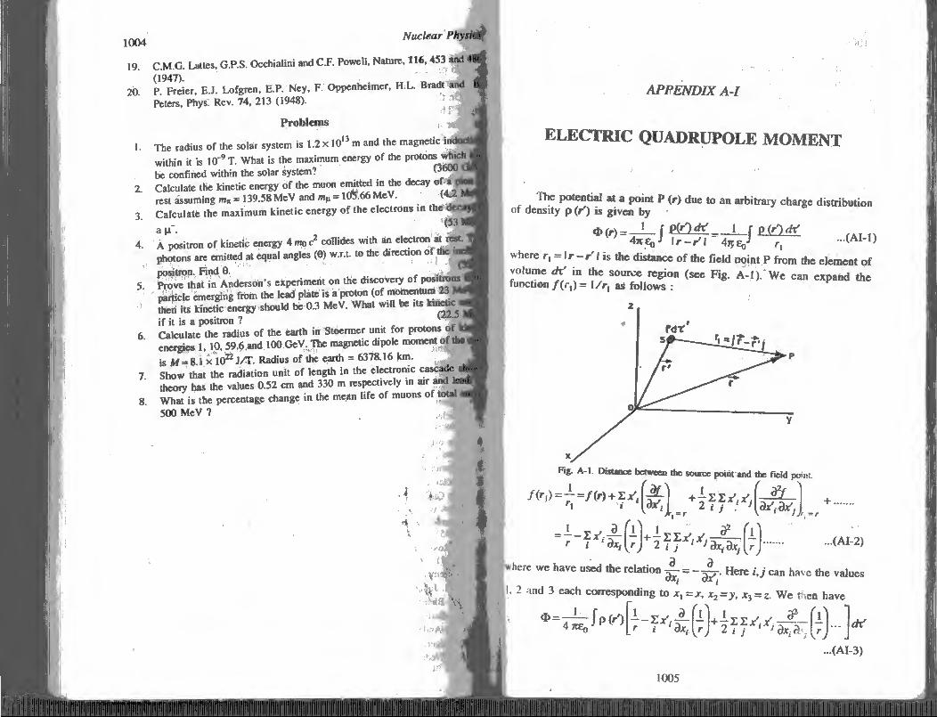
itial at a point P (r) due to an arbitrary charge distribution ') is given by

<*(r)= » rAlr lr-r'l AntJ r, •(AI‘1

r 1 is the distance of the field point P from the element of

the source region (see Fig. A-l). We can expand the

where we have used the relation ^ o

I. 2 and 3 each corresponding to

Here i,j can have the values

x, x2=y, x3 = z. We then have

1006 Nuclear Physic

The first and second terms in the above expansion give the potential* due to the electrip monopole (total charge) and the electric dipole IocuKhI

at the origin of the coordinate system which are not of interest for us if) the casp Of the nuclear charge distribution. The third term gives the potential due to the electric quadrupole located at the origin and is given

by

Since the integration is over the source coordinates xwhile th#

derivatives of 1/r are with respect to the coordinates of the field point (*,),

these can be taken out of the integral so that we can write

d>2 = -r- \ z s 3-4- Nip ('') *1 x'j ...(Al-5) 2 47teo 2 i j dxjdxj l r JJ 1

...(Al-3)

Now since 1/r is a solution of Laplace’s equation for all points except r = 0, we can write

HU - = ZX^ V [rj-rd^rjij^dx^r

We multiply the above expression by

1 -8,1 = 0 ..(Al-6>

and subtract it from Eq. (AI-5) which does not change the expression fo* 02. So we get

IX Z -4- (-|/p 00 Ox',x) - /2 8,y) dx' ...(Al-7) 2 4 hEq 6 i j axt axj [r )J 1

If we write

We get

Qij = J P (r') (3 x\ x/j - /2 8tj) dx'

._1_1 _ _ n ^ i = 4 JtEo 6 f j ^ Bxj d Xj

...(AI-8)

...(AI-9)

The nine quantities Qy constitute a tensor of rank 2 known as the

quadrupole moment tensor which can be written as

011 012 013

{Q}=' 02i Q22 Qn' — (AI-10)

Qi\. 032 033.

It is a symmetric tensor so that Qy = Qjt which reduces the number

of components to six. It can be shown that the sum of the diagonal elements (trace) is zero:

XQ„. = xjp(r') (3.x'2- r'2) dx'

leptric Quadrupole Moment 1CK)7

= Jp(r') (3X^-3j/W

\ w = J p (r') (3r'2 - 3r'2) dx’ = 0

\y<j|iave <2,, + 222 + G33 = 0 ...(AMI)

This means that only two of the diagonal components are dependent. This reduces the number of independent components from

ix to'five. v

Notv if wfc refer to the quadrupole moment tensor to the principal es, all the off-diagonal components vanish; Qtj = 0 for i *■ j. So we are

left with dnly fwo independent components of the quadrupole tensor. Finally if the charge distribution is axially symmetric as in the case

of an ellipsoid of revolution (spheroid), then Qu = Q22. This gives

033 =“ (0i 1 + 022) = - 2 Qu = - 2 e22 ...(AI-12)

Thus we are left with only one component of the quadrupole moment tensor Q = Q33 which is called the quadrupole moment of the charge

istribution. It is given by

0 - 033 = j P (O 0 Z.'2 - r'2) dx’ ...(AI-13)

For a system of point charges qa located at the points r 'a we have

Qij = ZqaOx'aix'aj-/2aSy) , r ...(AI-14)

For an axial distribution of charges we have

Qv = ZqaOz'2a-r'2a) ...(Al-15)

The above discussion is purely classical. Eq. (AI-14)dr (AI-15) gives

he intrinsic quadrupole moment Q0 of an axially symmetric charge

istribution. The measured value of the .quadrupole moment Q is usually

ifferent from Q0 because of the rules of space quantization in quantum

techanics.

To illustrate this we consider a very simple system consisting of two

qual charges q placed alo^g the 2-axis at the distance / from the origin

_n either side of the latter, z* is the body fixed axis of the charge system.

[Since r' = l for both the charges, the intrinsic quadrupole moment calculated with the help of Eq. (AI-15) comes to he

0q = QO l2 -l2) + q (3 l2 - /2) = 4 ql1

We now calculate the quadrupole moment Q referred to the space-fixed axis z.

Let / be the spin so that the magnitude of the angular momentum,

ording to quantum mechanics, is V7(/+ l) which iS>:along z'. Its

projection along some preferred direction z in space (wfiicft may be the

direction o' an applied electric field) is MU, where the (21+ 1) possible

yalues of M are /, 7 - 1, / - 2.— /. If (3 is the angle between z' and z, then (here are (21+ 1) possible values of B given by

Nuclear Physics

cos ft = |-^= ...(AI-16) W+ 1)

Since the maximum value of M-l, the minimum angle ftm between

and z is given by _

o / a/ /

Pm V/(/+1) V/+1 ...(AI-17)

Eq. (AI-15) can be used to find the quadrupole moment Q referred

to the space-fixed axis z for a given orientation ft of z' w.r.t. z :

Q = q (312 cos2 p - P) + q(3 ? cos2 0 - Z2)

= 2qf 3 M2

./(/+1) . ...(AI-18)

j£_I

i(i+1) 3 M2 — / (f + 1)

/(/+1)

For M = I, we get

It can be shown that Eq. (AI-19) can be applied to any chargr

distribution with an axial symmetry.

So we get, using Eq. (AI-13), •

...(AI-20)

Eq. (AI-20) is semi-classical since it does not take into account the

nuclear wave function. If we consider a nucleus in the shape of an

ellipsoid of revolution rotating in space, the angular momentum / has the

projection K upon the symmetry axis of the nucleus (see Fig. 2.9 tit

Ch. II). It is then possible to connect the electric quadrupole moment Q

referred to a space-fixed axis along which the nuclear spin / has the

component M - ! with the intrinsic quadrupole moment Qq referred to the

axis of symmetry from a knowledge of the wave functions of the rotating

ellipsoid. The result that one gets is*

...(AI-20)

3Ez-/(/+l) e = Qa ...(AI-21) u Wo(/+l)(2/+3) ■

This is the result quoted in Ch. II (see Eq. 2.12-12).

Energy of a charge distribution in an external electric field

Let $ be the potential from which the field E is derived f

E = - V <)>. If p denotes the charge density, then the energy of the charge

distribution in the field is

See Physics of the Nucleus by M.A. Preston, Ch IV See also Theoretical Nutt*#* Physics by Blatt and Weisskopff.

Electric Quadrupole Moment

^ U=jp(r)ty (r) dx ...(AI-22)

If we expand * (r) about the origin of the coordinate system, we can

'' 1 (d£.l X =<HO)-£x,(Ei)0--i:ix^k^ ••••

' i L t j \axi Jo

where v E,=- fr/dxj \ < * We then have .

’ • r T 1 I dEj l tU = \p(r) <KO)-i:x,(E,)0--IIx1.x.^

Writing

...(AI-23)

(7 = X Url we have

l/0 = Jp(r)<|>(0)<#t' = <fr (°> J P (r) dx’ = q if (0) ...(AI-24)

where q = \p(f)dxJ is the total charge of the distribution assumed

concentrated at the origin.

U, = - J p (r) X x, (Ei)0 <fx = -Z (£,)„ J p (r)xtdx

= -IPi(£<)o-~P ' ..(AI-25)

where p, = j p(r) x, dx is the i th component of the electric dipole moment

of the charge distribution, assumed concentrated at the origin.

Thus U0 and 17, are the energies of the point charge q and the dipole

of moment p located at the origin respectively.

The third term in the expansion gives

U2=-±lp(r)21x,Xj dx z I j V1 Jo

2 ' 1 I4**- n

...(AI-26)

Since the sources producing the field E are far removed from the

given charge distribution, we have

3E, 3Ei „ V-E-Zy1* E£^5jy=0

i oXj i j oXj

If we multiply this by p (r) ? 5,/6 and subtract from the integrand

in Eq. (AI-26), the value of U2 remains unchanged. Thus we get

Nuclear Physics

- _ uU

1 3£, f J p(r) (3 X'Xj-SS^dx ...(AI-27)

v 1 Jo In view of Eq. (AI-8), this can be written as

1 (be'

t'2 = ‘6ffe«('^J0 •<AI-28'

where QtJ represents the quadrupole moment tensor of rank 2. U2 gives the

quadruple contribution to the energy of the charge distribution, the quadrupole being assumed to be located at the origin.

p h "> *

APPENDIX A ll ?

THEORY OF SECTOR FOCUSED CYCLOTRONS

The principle of azimuthally varying field (AVF) or isochronous cyclotrons which finally led to the construction of sector focused cyclotrons discussed in § 12.15 was first proposed by L.D. Thomas in ___ ..... « l .• n.. *!__tkaon; r»f frtniQina

by the azimuthally varying magnetic field.* Referring to Fig. 12.17 in § 12.15 we note that if there are N hills

and N valleys and the magnetic field variation is sinusoidal, we can

express the field B (0) it an azimuth 0 by the following equation :

B (0) = (1 +/cos NQ) (AW-1)

where is the average guiding field and / is the peak flutt^r amplitude. B (0) = Bz is along z in the medium plane. This fluttering of the

field gives rise to a force qv /cos NQ on the orbiting particle which distorts the particle orbit. Instead of a closed circular orbit of radius 7? in a field which is the same at all azimuths, the orbit is now a curved

polygon as shown in Fig. 12.17c. Denoting by x the radial displacement from the constant radius orbit

due to the fluttering field, we can write the equation of motion as

mx = -qv/cos NQ tAu-Z)

It has a solution of the form

x = (fR/N2) cos N 0

Thus x has the same periodicity a» the magnetic field variation. The orbit extends beyond the ipean circle in the hill regions and lies within the

circle in the valley as can be seen in Fig. 12.17c.

The radial velocity vr of the particle is

vr = (0 • dx/dQ = - (vsfR/N) • sin IV 0 (AH-3)

where 0) is the angular velocity.

Since VxB = 0, we get

(V xB)r = (1/r) ■ dB /39 - dB^/dz = 0 (AII-4)

Hence the azimuthal component of the magnetic field is given by (writing

R for r)

* See The Principle of AVF Cyclotrons by C. Ambasankaran, S. Chatterjee and A.S.

Divatia in Physics News, Vol. 8, No. 3 (1977).

1012 Nuclear Physics

R „_i<^ Nfz . 6 dz'Z~rdd'Z~-R~Sm NQ CAD-S)

Due to the action of Be on the radial component vr of the velocity,

the particle experiences a force Fz in the vertical direction (see Fig. 12. l<vr in § 12.15). This is given by

Fz = -<!VrB0--quif2zsm2Ne Since B = mto/q, we then get

Fz = ~ nuo2f2z sin2 N 0 ...(AII-6)

^vanishes at the centres of the valleys (0 = Jt, 3jt,5ji etc.) and the hills

ft"0;-,2”,’4" ^dc.). ft is maximum at the hill-valley boundaries where , n/I’3K/2etc- This force ts always focusing. Since the oscillation frequency of the particles is small compared to the frequency of variation

of the field, we can take the mean value of sin 2 AO equal to - in the

expression for Fz so that we can write

< Fz>~ 2 m<£f2z ...(AII-7)

Apart from the action of Be on v, the radial component Br of the magnetic

field acting on the velocity component ve = r to also exerts a force F on

the particle in the vertical direction given by

F\ = gvBBr = qnoBr * ...(AH-8)

. dfl, dB where Br = —Z = — Z .(AH-9)

in view of the vanishing of the curl of B. If n denotes the average field index we can write

< Bz > - < B0 > ^ J ...(An-10)

where n > 0 since the field increases outwards (see § 12.8). n is given by

d<Bz>

We then get

<BZ>

dBz rz - qrta z = n Bzooqz = nmus2z

where we have put S.a) = mu>2/q

The equation of motion along z is then given by

2 + j^--«]a>2z = 0

...(AII-11)

...(All-12)

...(All-13)

We saw in § 12.7 that a magnetic field decreasing with increasing radius produces a net focusing of the beam in the z-direction. Hence the magnetic field Bz increasing outwards has a defocusing action on the

theory of Sector Focused Cyclotrons 1013

beam However, the combined actions of the azimuthal component Be and

ihe rad^l component Br of the field will produce net focusing due to

vertical oscillations if in Eq. All-13.

' /2/2 > n ...(All-14)

This means that for focusing, flutter amplitude/of the magnetic field

.ast be large enough to fulfil the condition (All-14). Since the angular [velocity (0 of the particle must remain constant for resonance condition to [hold the average magnetic field < Bz> at all azimuths must increase

according to the following relation

<iz> = <B0>Wl-P2 =<B0>Y ...(All-15)

_- where T=l/-Vl -p*.

Further to = v/r= Bc/r = constant = Mq (say)- ■

|So we have r= « “b I'Ve then get

d<Bz> d<B,>dB <«o>P

dr " ap dr (1-P2)3/2

Hso using Eqs. (All-15) and (AII-16) we have

<BZ> <Bo1<B0>

We then get from Eqs. (AII-17) and (AH-18)

r d<Bz> pc oibp<g0>ir?

<BZ> <%7 <Bo> = P2r2

So the focusing condition (AH-14) reduces to

f /L> .

.(AII-16)

...(AII-17)

...(All-18)

...(AH-19)

...(An-20)

The frequencies of the vertical and horizontal betatron oscillations depend not only on n but also on the azimuthal configuration of the magnetic field. The deperfdence of the frequency ratios V, - U)/co and

v =a>/0) on the structure of the magnetic field is very complex and

rigorous calculations of the orbits in the AVF machines can only be done

numerically with the help of computer. Writing the magnetic field at an arbitrary point in the median plane as

we can obtain the

0,0) = B0 j d>(r, (

he function <1> (r, 0) from the condition

2n Jo d> (r, 0) dQ = 1

...(AII-21)

...(AII-22)

Tlris leads to Eq (All-19) for the variation of the average field

< B, > vith r as given earlier.

Nuclear Physic#

We now introduce the/luster function F(r) defined as ' ^

,.(An-2.<

Further 'f ^ (r) denotes the angle made by the tangent to the spiral with the radial direption then it can be shown that to a first order of approximation*

V'2=1+" ...(All-24)

vl = -n + F (R)(l + l/2tan2Q ...(AII-25)

Thus for the radial oscillations the dependence is similar to that for a conventional cyclotron (see Eq. 12.7-10). The vertical focusing increases with F and with - ..'.s _ *

The function «!> (r, 6) for sinusoidal contours in purely radial sec tori' can be written as (see Eq. All-1)

<J>(r)=l+/cosWe ...(AII-26)

In this case, the flutter function F=f2/2 is a constant where /is the flutter amplitude. J

For spiral sectors and sinusoidal field variation d>(r, 0) can be written as

(r,e)=l+/c0s[tf{e-g(r)}] . ...(AII-27) where g(r) depends on the shape of the spiral. In this case also it is found F=f /2. ' ^ . , Tw°kmds of sPiral are generally used, the logarithmic spiral and the

Archimedian spiral, for which g{r) has the following forms :

For logarithmic spiral : g(r) = tan £ In (pr) ...(AII-28)

For Archimedian spiral : g(r) = p r = tan £ . .(An-29)

where p. is a constant.

The condition for isochronism of the particle motion and the accelerating voltage requires that the average field index n be a function ot the radius r. This variation can be expressed in terms of the energy E for any radius r as follows.** 62

- ~(An-3<»

a . .For better vertical focusing it is desirable to increase C and use the Archimedian spiral for which £ increases linearly with r (see above). For radial oscillations vr * y which shows that \r changes appreciably with

energy and leads to instability of the orbit for the integral resonance Vf z. this limits the energy of these cyclotrons to about y=2 or the kinetic energy T=E0 which is 940 MeV for protons.

A.V.F. cyclotrons have been built to produce intense meson beams Cmeson factories).

* ?ee PnnciPks of Particle Accelerators by Perisco, Ferrari and Seere ** See ibid.

1 i i ! lilillll i in i

m APPENDIX A-III

vTHEORY OF ALTERNATING GRADIENT (AO) FOCUSING USING QUADRUPOLE

' LENS SYSTEMS

(We shall consider the motion of a charged particle through an _zctrostatic guadrupole lens which consists of four electrodes with sections in the’shape of rectangular hyperbolas arranged symmetrically as shuvvn in Fig. 12.20a. The alternate electrodes are at (he potentials + V

End - V- The beam passes along the axis of the electrode system (z-axis). ■Tie transverse field Ez has the form Ex = -Gex in this region, G being I constant. Since the field has no Z-component, the condition V • E-0 Eves Ev = + Gey. This makes it possible to focus the beam strongly in the

Ez plane. At\he same time there will be strong defocusing in the Ez plane. If the beam now passes through a second e.s. quadruple lens Eith reversed gradients in which Ex = + Gex and Ey = -Ge y, there will be

Eefocusing in the x-z plane and focusing in the y-z plane. However there Is net focusing in both the planes for the beam passing through the two

nses successively (see Fig. 12.20b). The above field pattern is derivable from a potential of the form

V=(Gt/2)(x1-y2) ...(AIII-1)

he equipotentials are rectangular hyperbolas.

We now analyze the motion of the particle in such a field. The

quation of motion in the x-z plane in the first lens can be written as

mix-- qGex, x + p2x + 0, |52 = qG/m ...(AIII-2)

i he solution of this equation is of the form

x = Xq cos Pf + (xo/P) sin Pt

= x0 cos kz + (xo/to) sin kz ...(AIII-3)

x0 and x0 are the initial position and transverse velocity respectively. Here

we have used the relation z = vt, v being the velocity of the ion beam along

k = (qGe/ mv2)1/2

We then get for the exit point z = a from the field

...(AIII-4)

1015

miiaiiimiininiiiiiiSHiiiiiiuiiiHiifHiMTiiiitiiiiiiiMi!

Nuclear Physic

Also *=-‘bc«*a + (V*v)sinfez -.(AHI-S) so x/v = - kxQ sin ka + (Xq/v) cos ka (Amftl

I he two equations (AIII-5) anH rAm , u- l. *’ transverse velocity at the exi* i . w^,c^ S,ye the position aritl yield the * —*■ fon,»

I* U Xl/^slntoit^ f l*/lT M«n*B cosfai| ji^v --(AIU-7)

In the second field region since the tion g-~ ■ solution of Rn /aih - ’ nCC th sgn of G' ,s ^versed, the

sinusoidal functions so that"we fU"Ct'0nS in Place of ***

_ cosh ka (l/k) sinh jta! 1 Jd j I | k sinh Jta cosh Jta j 1 Vv| ...(AIII-8)

regions successively become 4 t •

x \ -\ cosh ka (i/k) sinh fail I

— J l-*s= M,^q |£| *b (cosh ta cos ka — sinh Jta sin /ta) +

, = . . . , (V*v)(cosh fci sin fci + sinh Jta cos fai) * (sinh ka cos ka- cosh Jta sin Jta) +

(Vv Kcosh ka cos ka + sinh far sin ka) j

Similarly we g« in the „ plane, * fo||0„ing . ~ 'AnM>

yo (cosh ka cos ka + sinh ka sin ka) +•

L/J= . a. . . , 6-(/*vXcosh *a sin + Sinh ka cos ka) \yv I *yo(smhfaj cos ka- cosh ka sin ka) +

* ^ Wcosh ka cos ka- sinh ka sin ka)

qu.d™p'oleate„VL1^“°S ^ T™* »*.» tê'tie discussed above. In this case the quadrupole Ienses product of the particle velStv ® grad,ent is by the AG accelerators, the particles na« êld 8rad*ent In actual elements. The matrix thr°Ugh many ânds of AG yield any meaningful result^ h beCOmes to° complicated to

S °f is

z:*: %*£

coska (I /A) sin ka x0 * sin ka cos ka Xq/v

i

FTheory of Alternating Gradient 1017

transformation matrices for a magnetic quadrupole lens as given below. If

we write'’" .

k = (qGJmv)w2

cos ka sin (ka)/k

v ~ -k sin ka cos ka

...(AIII-11)

...(AIII-12)

cosh ka

...(Ain-14)

...(Am-15)

..(AIH-16)

| ' , . . sinhta v I i and, i = C°Shka k ■ * ...(AIII-13)

^ y v k sinh ka cosh Jta

r for motions in the focusing and defocusing planes respectively. For the basic triplet of lenses as stated above, the transformation

matrix for finding the final position and transverse velocity at the exit end in the case when the first element is focusing is given by

cos(Jta/2) [sin (Jta/2)]/Jt coshta [sinh (ka))/k x — Jfc sin (Jta/2) cos (Jta/2) k sinh ka coshta

cos (ka/2) [sin (ka/2)]/k /A ITT 141 -k sin (Jta/2) cos (ka/2) '' ;

After multiplication of the three matrices, the resultant matrix becomes

cosh Jta cos ka l/k (sinh ka + cosh ka sin ka) (Affl-15) k (sinh ka — cosh Jta sin ka) cosh ka cos ka

This matrix can be written as

cos [i (1/if) sinp ..(AIH46) - K sin p cos [t

provided the product cosh ka cos Jta lies between - 1 and + 1. i.e.,

— 1 < cosh Jta cos Jta < +1 ...(AIII-17)

In Eq. (Am-16) we have written cos p = cos Jta cosh Jta „.(AIII-18)

and K2 = Jfc2(l - cosh*Jta cos2 Jta)/(sinhJta + cosh ka sin ka)2 ...(AIII-19)

As long as the condition (AIII-17) given above is fulfilled, both p and K are real and the matrix (AIII-16) is the proper transformation matrix for obtaining the exit position and transverse velocity. Comparing with the focusing matrix (Am-12), we conclude that the matrix (AIII-16) is also a focusing matrix so that there is net focusing of the beam of particles in going through the basic triplet of lenses considered here.

If, then, a large number of the sequences of the basic triplets as above are added one after another, we shall get net focusing provided the condition (AIII-17) is fulfilled. This is known as the criterion of stability.

The above analysis applies to both linear and circular systems. In the circular system, like the AG synchrotron, the betatron oscillations are along the radial direction (x) about the closed orbit of radius R and in the

APPENDIX A-IV 1018 Nuclear Phytlyt

vertical direction (y) about the median plane. For a magnetic field variation with a field index

\n\ = ^ B dr

the equations of motion in the radial direction for two consecutive sector* are*

d2x/ds2 + (n- l)/n k2 x = 0 a , , ...(AIII-20) and d x/ds2-{n+\)/n k2x = 0 ...(A1II-2I) where k has been defined above, j is the distance measured along the

In the AG machines n is large (n ~ 100 or more). So the above equations reduces tf>

cfx/ds2 + k2x = 0 ...(AIII-22) since n and the field gradient have opposite signs in the two cases Thl equatmn of motion in the vertical direction has the exact form given by tq. (AIII-22). Thus the oscillation wavelengths are equal in the tw# cases : k.. — k

Now the quantity p given in Eq. (AIII-18) is the phase shift in th# betatron oscillation per pair of quadrupoles. If there are N pairs

SmnSh 6 u°F 2N AG-quadruP°les, then the total phase shill I ound the orbit will be Mp. If this is an integral multiple of 2n, there will

be an integral number of betatron oscillations per revolution which leads to orbit instability. Such instabilities are avoided by calculating theoretically the locations of these resonances and then taking necessary steps to operate in regions between the resonance lines.

See Particle Accelators by M.S. Livingston and I P Rl™,»

D VATION OF RARITA - SCHWINGER

1 EQUATION

i For a mixture of S and D states, the wave function is

:•/ ’ t j- 5 + <j>D

a where the S-state wave function is

<t>s = v(r)

'101

and the D- state wave function is

<j> =^My> D r 121

The Hamiltonian operator for the two body systeip can be written as [ (for M] <= N2 = M)

Hsd-^--fV2 + V M

: n H i 3 a r2 3 r dr ?

where S12 is the tensor operator. )

? 3 V 1 a = ——r sin 0 +

■te¥cW+ Vf(r)Sl

.‘f j t

30 sin 2 0 3 ® sin0 90

It can be easily seen that 1 3 2 3 v(r) v" (r) o -V ' -v

r2 dr dr r (AIV-1)

, 1 3 7 3 (0 (r) _ o)"(r) r1 dr dr r r

(AIV-2)

The operator a2 operating on the spin angular part of the wave

function gives

a 2 yljLs = I‘(L+ 1) //ls (AIV-3)

where L can have the two values L = 0 (S—state) and L — 2 (D— state). Substituting in the wave equation, we get

1019

,®L_V i ) . ^2 to(r) 2(2+1).., A# r )I<JI ^ 121 +T7—' ,+ M r

(Vc(r) + Vr[rJ^-£ ){ ^ y,«#I + ^ y'j2| f = 0

Collecting the terms in K,'ol and K,'2|, we get

-Afvly. 1 A 6o\ ^,2, M\r y"")-m v® —J—+

\vc (r) + VT (r) St2 - £} y,'0I + ^ K,'2tJ = 0 ...(AIV4)

Because of the orthogonality of the spherical harmonics, we then gel

~ M di* + Vc W “ Ev = ~ Vr(r) ® ...(AIV-5)

T^fd2 (a 6ti)'l A/ j_2 j +^c(r)^-2Vr(r)(o-Fxo = —'I^VT(r)v

... (AIV-6) where )ve have made use of the results (see. Eqs. 17.12-16 and 17-12-17)

^12 ^ioi - ^ Yl: ... (AIV -7)

...(AIV - H) ^12 ^121 - ^ioi - 2y,2, ...(AIV - K

Proof of the relations (17.12-16) and (17.12-17\

Let Sn y/o, = a + b Y'2\

It may be noted that does not contain 0 or O. When averagctl

over the angles < $i2 > d>=0 and the average on the l.h.s. <Sf}

K!oi > = r.h.s. since Y^ does not contain 0 and 4>, the average

of the first term is not zero and hence we should put b = 0. The above relationship is valid for all 0 and <b. In particular, if we choose 0 = 0, we

get y22(0 = O) = y2<e=°) = 0, while y°(e = 0) = V^ 2 4n

On the other hand

V0 = 0) = 3 (of x rQ ) (^ • r0 ) - of-6^

^t2 ^101 - (30lz ~ ^

= ^-(3 «. «2-a, “2) for =0

Againy,1L (0 = 0)= Y v~'Y r° + Y i 121 ’ M0 »*1 10 21Z' V10 20?

...(AIV-4

Derivation of Rarita - Schwinger Equation IUZ1

l)ct,«2

V 2tyx2

V321T _a/3jt M VT 2a,«2

1 1 20t2«2

5,2y,ot=>/8 y.'j, for 0 = 0

.-. b = >IS and

5.,y.!».=V8 y,'21 for all 0 J12 101

...(AIV-10)

'To find Sy, y|21 we choose 0 = n/2 and <t> = 0 (x - direction).

cos 0 = 0, sin 0=1, cos 0= 1, sin <t> = 0

S12 = 3 (o| - r0) (a2 r0-) — o|, o2

= 3<Jlx Ofr -

A = «n2 e exP (») =

= sin 0 cos 0 exp (i d>) = 0 oTC

. (AIV - 11)

(AIV - 12)

... (AIV-13)

...(AIV-14)

,.JJT 2~ V8*

r/xi'-VI’

=^/m»^*“^10'^16n Wiaj

yl r 12*

(AIV-15)

5|2 y,21 " (3®U ®2* ®l ’ **2)

» - _

-«|«2 3 P2

l32^ + l^TJ v > 3P,P2 «1*2 9a1<X2 3 P1P2

l^+l327 + l327~l32^

10 a,otj 6fi,P2

=^32r_^r

8 0,04

V32 n + 2

$12 ^121 =V8 y' -2y;21

j" 0,02 3 P, p2"

(V32 n V 32 it (AIV-16)

...(AIV-17)

APPENDIX A-V ■ '!* i V •

VECTOR ADDITION OF ANGULAR MOMENTA: CLEBSCH GORDAN

COEFFICIENTS

angular S£i“m v««o" “ ?<»"P°'"’d W“ of the system Thus thp nrhif,1 eJhe resultant total angular momentum

electron combine to producethl ?otal?u“ 2*^”^ *”L“°”“ gives rise to the fine structure of the affeiiic snectral lines i„rh+ S Wh'uh

55a3F»^»^=SS Consider two angular momenta /, and J2 which separately satisfy the

commutation r„,es [7,./,) =0 etc.. and which mutually commit,eu!

m' 6 the slmultaneous eigenfunction of the operators j] and J,

m “fvV0 thC reSpCCtive e*£envalues 7, (/, + I) and «, where and J .™8f be ,ntegers or half-°dd integers such that -j,<m <+j Similarly Y^ ,S the simultaneous eigenfunction of ;22 and Ju belonging

to the respective eigenvalues j2(/2 + 1) and m2 where -;2 <*,.< + /,

The product of the wave functions Yy. (ll| , y is an eigenfunction of

ZJS3ZLZZtotal angular m“m * with the

* ~ «-«■ «-

two angular momenta J, and J2 „ is, how.™ VosllbleTform ££ combinations of the products y y * • , proaucts Yjy Wj which are simultaneous

ergcnfunctions of / and 7, wMf'dla eigenvalues 7(7+1, and «

respectively. Denoting these eigenfunctions by ip"^ we then have

j 1 72

<AV‘I)

1022

109^ Vector Addition of Angular Momenta

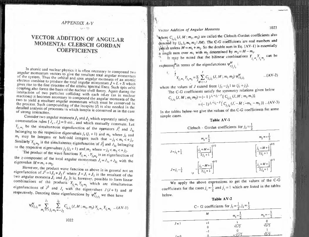
’*vhere C; j (J, M ; m,, m2) are called the Clebsch-Gordan coefficients also

denoted by (/, A tn2l JM). The C-G coefficients are real numbers and

yabish unless M = m, + m2. So the double sum in Eq. (AV-1) is essentially

a single sum over m, with m2 determined by m2 = M-m,. A it may be noted that the bilinear combinations T „ can be

ex firessed*in terms of the eigenfunctions ^ . :

J kJ-7

...(AV-2)

where the values of J extend from \j\ —fal to (/i +J2)- The C-G coefficients satisfy the symmetry relations given below

Cj j2(J, M ; m, mf) = (- 1 )J,+Jl~7[c/2j1 (J>M ; m2mi)l

= (_ j)i\*h-}\ Cjj2 (J, - M ; -m, - m2)] ...(AV-3)

In the tables below we give the values of the C-G coefficients for some

simple cases. Table AV-1

Clebsch - Gordan coefficients for jz = ~_

J=J,+12

J-Jri

1 2j, +1

Jr*+i

i,L 2yi + 1

2;, + i

2>! + 1

We apply the above expressions to get the values of the C-G

coefficients for the cases;, ={ and;, = 1 which are listed in the tables

below. Table AV-2

C— G coefficients for 72 - 2

i = n

J= 3/2

/= 1/2

Table AV-3

Nuclear Physics

G coefficients for h ~ l./2 = j

M --

"2=5 «2=-i

3/2 1 0 + 1/2 <275 <i7T -1/2 <U5 <275 -3/2 0 i + 1/2 -<V3 -1/2 -<275 <575

Nuclear physics by Blatt and Weisskoff w h ca*

v*lu's ”f "* CO. coefficients m 5 Kam1" °f "" abo,e

*

..Mill.I.lilliliiM—■

\ \ APPENDIX A-VI

THEORY OF GEOMAGNETIC EFFECTS OF V THE COSMIC RAYS

Consider the motion of a charged cosmic ray particle of relativistic mass m carrying a charge q coming from infinity towards the earth.

The magnetic field of the earth is equivalent to that due to a

magnetic dipole of moment M = 8.1 x 1022 J/T located near the centre of the earth, the dipole axis pointing south. Using spherical polar coordinates r, X and <|> shown in Fig. 19.4, we can write the velocity of the particle in terms of the components vr = r, = r X and = r cos X ■ d> and the unit

vectors er ex and along r ,X and <b respectively. We get

v='rer + rXex + r cosXOe^ ..(AVI-1)

The magnetic vector potential due to the dipole of the earth is

4 Jt _

Mo M cos X a ...(AVI-2)

The magnetic induction is Eg UnM

B=VxA=--j (- 2 sin X er + cos A. • e...(AVI-3) 4 it r

The horizontal component of the earth’s magnetic induction at the equator is Bt=0.31 x 10“4 T. If p denotes the relativistic momentum and jp the

radius of curvature of a particle of unit electronic charge e in this field we can write *

Be v = m v2/p

B p = e e

pc = Bpec ’ ...(AVI-4)

The momentum of the particle for which p = re (the earth’s radius) is

then given by

pc = Bre ec

- 0.31 x 10" 4 x 6.378 x 106 x 1.6 x 10"19 x 3 x 108

= 59.6 GeV

1025

Nuclear I’hwo *

Thus pc is large compared to the rest energy of the particle, be it,#

proton (rest energy 0.938 GeV) or an electron (0.51 x 1(T3 GeV). Hcne# pc can be taken to be equal to the total energy (or kinetic energy) of ih« particle. More accurate estimates give the kinetic energies of the electron and the proton to be 59.6*GeV and 58.5 GeV respectively for the abov# value of pc.

In a static magnetic field there is no change in the velocity v of th« particle or in its energy E and momentum p. The Lagrangian of such a particle is*

L = -m0c2 Vl -p2 +e(A ■ v) ...(AVI-S)

Using Eqs. AVI-1 and AVI-2 we get

L = - m0cz P2 +'C p0 Me cos2 A.

...(AVI-ft)

Since L is independent of <)) we get from the Lagrangian equation of motion

= = 0 ...(AVI-7)

so that

dt di> d <j> dL

P* = 3^ ~ constant

...(AVI-7)

...(AVI-8)

dL 2 d ,.r. FF 3v *VoMe 7 ^ = -m0e^(V1^P)^ + —cos X ...(AVI-9)

We get finally

a<T ^ 19(p

v2 = r2 + r2 X2 + r2 cos2 A, <j>2

9v r2 cos2 A, d>

d<|> v

...(AVI-10)

...(AVI-11)

V, ...... r2 cos2 A. .i Po Me cos2 A. . P* = P -+ - ...(AVI-12)

* L v 4nrp J

Since p^ and p are both constant, we get

P» r2 cos2 A. ; Po Me cos2 . —* =-<b +---= constant ...(AV-13) p V 4 71 r p

Let 0 be the angle made by the trajectory of the particle in space with the meridian plane. 9 will be taken positive if the orbit crosses the meridian plane in the direction of increasing <|> so that sin 0 is equal to the <j)-component of a unit vector in the direction of the velocity. Hence

„ v* r cos A. • (|) sin0 = -I =-31 ...(AVI-14)

...(AVI-12)

...(AVI-14)

Then from Eq. (AVI-1 we get

P* - . „ Po Me cos2 A. - - r cos A sin 0 +---; p 4 n rp

...(AVI-15)

Theory of Geomagnetic Effects of the Cosmic Rays

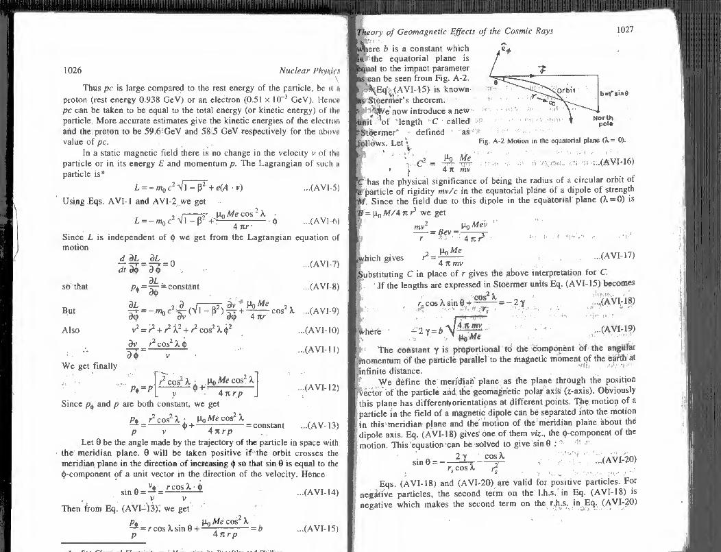
[phVe b is a constant which in the equatorial plane is f ■qua) to the impact parameter / ks can be seen from Fig. A-2. ■r< -^q. (AVI-15) is known ' jfe Stbermeir’s theorem. P yte now introduce a new knit oV length C called f* iStoermer’ defined as ** ■follows Let \ Fig. A-2 Motion in the equatorial plane (X= 0).

bef *in0

..0 o viiiSN!. at 'II i.i(AVM6) • j 4 7t mv

t has the physical significance of being the radius of a circular orbit of Particle of rigidity mv/c in the equatorial plane of a dipole of strength Wt\ Since the field due to this dipole in the equatorial plane (A. = 0) is

= p0 Af/4 n r we get

mv2 „ PoMev

9Me .'i In Thte emhktant Y is proportional t6 the Component of the ntthfar tnomentum of the particle parallel to the magnetic moment of the earth at

infinite distance. We define the meridian plane as the plane through the position

Vector of the particle and the geomagnetic polar axis (z-axis). Obviously this plane has different orientations at different points. The motion of a particle in the field of a magnetic dipole can be separated into the motion in this meridian plane and the motion of the meridian plane about the dipole axis. Eq. (AVI-18) gives one of them viz., the ^-component of the


Where b is a constant which In the equatorial plane is t fcqual to the impact parameter /

■s can be seen from Fig. A-2.

I; \Eq. (AVI-15) is known

I^Stoemter’s theorem. *5

p JliWe now introduce a new •* •

nnit ‘of 'length C called ^ ' - i t?

pStoermer’ defined as '$

follows. LetV Rg- A-2 Motion in the e I s • ' ;

V c2 » — r.-«, 6 vs;Ai!- ttt n ;..(AVM6) • ^ 4it mv

fc has the physical significance of being the radius of a circular orbit of «IS particle of rigidity mv/c in the equatorial plane of a dipole of strength ■if. Since the field due to this dipole in the equatorial plane (X = 0) is

?B = |i0 M/4 n r3 we get

mv2 „ \ioMev ‘

Orbit b=f sin6

ivhich gives r =-- ...(AVl-i i) f 4 7t mv

Substituting C in place of r gives the above interpretation for C.

If the lengths are expressed in Stoermer units Eq. (AVI-15) becomes

... i • n . cos2X._ - r*VT_ 1

,Z 1 ” Ho Ate ’

p i The constant y is proportional to the Component of the angular

momentum of the particle parallel to the magnetic moment of the earth at

infinite distance. We define the meridian plane as the plane through the position

vector of the particle and the geomagnetic polar axis (z-axis). Obviously

this plane has differenborientations at different points. The motion of a

particle in the field of a magnetic dipole can be separated into the motion

in this meridian plane and the motion of the meridian plane about the

dipole axis. Eq. (AVI-18) gives one of them viz., the ^-component of the

motion. This equation can be solved to give sinG : ' »i3 -

*».~2xizssg . • ...(avi-20) r, cos A, C

; 1 J •; •• 'i „ ■' .' Eqs. (AVI-18) and (AVI-20) are valid for positive particles. For

negative particles, the second term on the l.h.s. in Eq. (AVI-18) is

negative which makes the second term on the r.h.s. in Eq. (AVI-20)

' Nuclear Phyxitl

positive. For a given y the regions of the meridian plane for which

I sin 8 I > 1 are forbidden for the particles. Only the regions for which

I sin 8 I < 1 are allowed. Even in these allowed regions the particles cannot

be everywhere. The allowed regions which extend to infinity are available Mi

the cosmic ray particles. However, those allowed regions isolated from

infinity by forbidden regions are not available to the cosmic ray particle*

Only high energy particles shot from the earth can circulate in these region*

For r, = 1 the radius of the particle trajectory p - the radius of the

earth. This happens for the particle momentum p = 59.6 GeV/c (sec Bq,

AVI-4). A close look at Eq. (AVI-18) or (AVI-20) shows that for

*> 1 the particle can come to the earth from any direction.

For rs < 1, pc < 59.6 GeV, the particles cannot reach the cailli

from all directions. Detailed calculation shows that if y > - 1 for positive

particles, the particles are still observable. On the other hand for

y<+ 1, the particles cannot reach the earth from any detection. The

observable values of sinG are determined by the condition (for y>- |)

■ a cos A 6 7^1 7~ ...(avi-21)

€ ' e

The limiting value of the angle is then given by (for positive particleii)

• n 2 cos A , sme‘=^X—pr ...(avi-22)

f 'e f

The complement of the critical angle 0C is equal Jo the semivertical angle

of a cone known as the Stoermer cone with axis perpendicular to the meridian plane such that no particle is able to arrive from infinity at the observation point along directions within this cone. Figs. 19.5a and b show the Stoermer cones for positive and negative particles respectively The planes are the horizontal planes at the point of observation P. For positive particles all directions east of the cone such as PA in (a) are forbidden. Similarly for the negative particles all directions west of the cone in (b) such as PA are forbidden. Thus the directions such as PB in both the figures are allowed. The limiting values of the momenta for given 0 and A are determined as follows.*

Since the radius of the earth is 6.378 x 10^ m its value in Stoermci unit can be written as (using Eq. AVI-16)

6.378 xlO6 6.378 xlO6^ .

e >7C V (p 0 Me/A re) °'

where pc is in GeV. This gives pc = 59.61*.

The inequality (AVI-21) gives

^ 1 — Vl - cos a cos3A f > . cos a cos A ...(AVI-23)

See Nuclear Physics by Enrico Fermi.

Hiiiiiiii.iiminiunriiHiiMii


where a = Jt/2-0. Hence using Eq. (AVI-23) we get _. _ -.9

„ , 1 - V1 - cos a cos? A :> 59.6 -r-

cos a cos A ...(AVI-24)

For particles in the meridian plane (sin 0 = 0), this reduces to

■t{ ' pc > 14.9 cos4 A GeV ,..(AVI-24a) <t ■%

Table AVI-1 gives the minimum momenta in GeV/c for positive

particles which can reach the earth from different directions at different

latitudes. * » ’ Table AVI-1

Direction j of arrival

c pm in in GeV at X cos a

3° 30° 45° 60° 90°

West -i 10.2 6.4 3.1 0.9 0

Zenith 0 14.9 8.4 3.7 0.93 0

East +1 59.6 13.2 4.6 1.0 0

0 2 4 t 8 10 12 It It II 20

BRxNf’tesla-m J Fig. A-3. Variation of the half angle a of the Stoermer cone with the magnetic

rigidity Bp,

Fig. A-3 shows the variation of the half angle a of the Stoermer cone

with the magnetic rigidity Bp which is measure of the particle energy. For

example at A = 20°, a = 180° for Bp = 28T-m. So all directions are

forbidden for particles of the above magnetic rigidity or less. On the other

hand for Bp = 78T-m, a = 0°, so that all directions of approach are

possible for particles of this magnetic rigidity or greater.

The general conclusion that one can reach is that the positively charged

primary cosmic rays should arrive at a place in smaller numbers from the east

than from the west, the Stoermer cones pointing east for them. For negatively

charged primary cosmic rays just the opposite is true. They should arrive in

greater number from the east than from the west. ,

APPENDIX A-VII

SOME FUNDAMENTAL CONSTANTS

Velocity light in vacuum (c)

Permeability of free space (po)

Permittivity of free space (e-o)

Electronic charge (e)

Avogadro number (No)

Specific charge of electron (e/m,)

Planck's constant (A)

Ti =(h/2n)

Boltzmann constant (k)

Compton wavelength for electron (A,c)

Electron volt (eV)

Atomic mass unit (u)

Electron rest mass (m,)

" .? " :i

Proton rest mass (Mp)

Neutron rest mass (M„)

Proton to electron mass ratio ,

Bohr magneton (p«) * •* ’ ,.

Nuclear magneton (py)

Classical electron radius (r,)

Bohr radius (do)

Rydberg constant for infinite mass (/?_)

Fine structure constant (a) g-factor for proton (gp,)

g-factor for neutron (g„)

Gravitational constant (G)

1030

2.997925 x 108 m/s

4itx 10'7 H/m

' 8 85419 x 10 '12 F/m

1.60219X 10'I9C

6.02205 x 1023 molecules per mole

1.758805x 10" C/kg

6.62618 x 10”34 Js

1.05459 x 10'34 Js

1.3807 x 10“23 J/K

2.42631 x 10'12 m

1 eV = 1.60219x 10'I9J

lu= 1.6606x10'27 kg = 931.50 lyieV

9.10953 x 10'3lkg

5.48580 x 10'4u

5.11003 xift^eV

1.67265 x 10'27 kg 1.0072765 u

. i. 938.280 MeV

' 1.67495x10' 27 kg 1.008665 u 939.573 MeV

1836.15

9.2741 x 10' 24 J/T

5.05082 x 1(T 27 J/r

2.81794 x 10'15 m

5.29177 x 10'" m

1.0973732 x 107m~‘

1/137.0360 5.586

- 3.8262

6.6720 x 10'11 Nm2/kg2

The modified long form periodic table.

APPENDIX A-IX

PROPERTIES OF STABLE ISOTOPES*

The atomic masses are given in 12 C scaie. The star (*) marked isotopes arc radioactive

Element Symbol z A Relative Abundance (%)

Atomic Mass i

Neutron n 0 1 1.008 665 Hydrogen H 1 I 99.99 1.007 825

2 0.01 2.014 102 Helium He 2 3 1.3 x 10_< 3.016 030

4 100 4.002 603 Lithium Li 3 6 7.4 6.015 123

7 92.6 7.016005 Beryllium Be 4 9 too 9.012 183 Boron B 5 10 19.6 10.012939

11 80.4 11.009 305 Carbon C 6 12 98.9 12.000000

13 1.1 13.003 355 Nitrogen N 7 14 99.6 14.003074

15 0.4 15.000 109 Oxygen O 8 16 99.76 15.994915

17 0.04 16.999133 • '• ' 18 0.20 17.999 160

Fluorine F 9 19 100 18 998 405 Neon Ne 10 20 90.9 19.992 440

21 0.3 20.993 847 22 8.8 21.991 385

Sodium Na 11 23 100 22.989 770 Magnesium Mg 12 24 78.8 23.985 044

25. 10.2 24.985 839 26 11.1 25.982 594

Aluminium A1 13 27 100 26.981 541 Silicon Si 14 28 92.2 27.976 929

29 4.7 28.976 497 30 3.1 29.973 772

Phosphorus P 15 31 100 30.973 763 Sulphur S 16 32 95.0 31.972073

Properties of Stable Isotopes 1033

\ Element Symbol Z A Relative Abundance (%)

Atomic Mass

ip 34 4.2 33.967 870

36 0.01 35.967 079

Chlorine Cl 17 35 75.5 34.968 854

A V 37 24.5 36.965 903

-T,

Ar 18 36 0.34 35.967 547

38 0.06 37.962 733

40 99.6 39.962 384

Potassium K 19 39 93.1 38.963 709 * %

. * 40* 0.012 39.964 000

41 6.9 40.961 827

Calcium

' r

Ca 20 40

42

97.0

0.6

39.962 592

41.958 628

43 0.1 42.958 777

- - 44 2.1 43.955 488

46 0.003 45.953 689

48 0.2 47.952526

Scandium Sc 21 45 100 44.955 917

Titanium Ti 22 46 8.0 45.952 630

47 7.3 46.951 767

48 74.0 47.947 949

49 5.5 48.947 872

50 5.2 49.944 784

Vanadium V 23 50* 0.25 49.947164

51 99.75 50.943964

Chromium Cr 24 50 4.3 49.946049 X V- ? ■ a >

52 83.8 51.940510

53 9.5 52.940651

54 2.4 53.938881

Manganese Mn 25 55 100 54.938046

Iron Be 26 54 5.8 53.939 612

56 91.7 55.934 934 T« •-1< • 57 2.2 56.935391 i .a

58 0.3 57.933 275

Cobalt Co 27 59 100 58.933 188

Nickel Ni W 28 58 67.8 57.935 336 f £*. •

60 26.2 59.930780 s 61 1.2 60.931050

62 3.7 61.928 340

64 1.1 63.927 956

Copper Cu 29 63 69.1 62.929590

[: f ' 65 30.9 64.927 789

Zinc Zn 30 64 48.9 63.929 140

66 27.8 65.926040

67_ 4.1 66.927 132

\ Properties of Stable Isotopes 1035

j Element A

Symbol Z A .. RTiVtt^ ^mic Men (u) Abundance (%)

T(±hne(him Tc 43 No stable isotopes

Ruthenium Ru 44 96 5.6 95.907 598

98 1.9 97.905 289

99 12.7 98.905 937

■v 100 12.6 99.904 217

. V 101 17.1 100.905 577 » 102 31.6 101.904 348

* } 104 18.5 103.905 428

Rhodium Rh 45 103 100 102.905 512

Palladium Pd 46 102 1.0 101.905 607

104 11.0 103.904 014

105 22.2 104.905 086

106 27.3 105.903 487

108 26.7 107.903 891

110 11.8 109.905 164

Silver Ag 47 107 51.4 106.905 091

109 48.6 108.904 755

Cadmium Cd 48 106 1.2 105.906 463

108 0.9 107.904 189

110 12.4 109.903 010

111 12.7 110.904 186 *’’• j 112 24.1 111.902763

f 13 12.3 112.904 407

114 28.8 113.903 367 ' • :yV.*Vr •

116 7.6 115.904 762

Indium r‘ ? In 49 113 4.3 112.904 089

115* 95.7 114.903 875

Tin Sn 50 112 1.0 Ml.904 834

114 0.6 113.902776

115 0.3 114.903 353

ii t 116 14.2 115.901 748

117 7.6 116.902 961

118 24.0 117.901 613

119 8.6 118.903 316

120 33.0 119.902 207

122 4.7 121.903 451

124 6.0 123.905 283

Antimony Sb 51 121 57.3 120.903 822

123

120

122

123

124

175

42.7

0.1

2.4

0.9

4.6 7n

122.904 220

119.904 024

121.903 056

122.904 282

123.902 830 17a anA iif.

.

Tellurium Te 52

Element Symbol z A Relative

Abundance (%) Atomic Mass (u)

126 18.7 125.903 312

128 31.8 127.904 468

130 34.5 129.906 232

Iodine 1 53 127 100 126.904 476

Xenon Xe 54 124 0.1 123.90 612

126 0.1 125.904 279

128 1.9 127.903 532 i , . ■ f 129 26.4 128.904 784

130 4.1 129.903 511

131 21.2 130.905 085

132 26.9 131.904 157

134 10.4 133.905 398

136 8.9 135.907 222

Caesium Cs 55 133 100 132.905 436

Barium Ba 56 130 0.1 129.906 284

132 0.2 131.905 045

134 2.6 133.904 493

135 6.7 134.905 671

136 8.1 135.904 559

137 11.9 136.905 815

138 70.4 137.905 235

Lanthanum La 57 138* 0.1 137.907 161

139 99.9 138.906403

Cerium Ce 58 136 0.2 135.907 180

138 0.2 137.906 027

140 88.5 139.905484

142* 11.1 141.909 300

Praseodymium Pr 59 141 100 140.907 698

Neodymium Nd 60 142 27.3 141.907 766 - V- i ' 143 12.3 142.909 856

144* 23.8 143.910129

145 8.3 144.912610

146 17.1 145.913 153 i

148 5.7 147.916 929

150 5.5 149.920 921

Promethium Pm 61 No stable isotopes

Samarium Sm 62 144 3.1 143.912074

147* 15.1 146.914 925

148 11.3 147.914 851

> 149 14.0 148.917 211 ■ *■ 150 7.5 149.917 303

■ i 152 26.6 151.919755

154 22.4 153.922 222

1 Euroi

Properties of Stable Isotopes

|< Element Symbol Z A Relative

Abundance (%) Atomic Mass (u)

\ % 153 52.2 152.921 260

Gadolinium « Gd 64 152 0.2 151.919 817 154 2.2 153.920 891 155 15.1 154.922 636 156 20.6 155.922 143

I *. X v

157 15.7 156.923 972 4

158 24.5 157.924 123 160 21.7 159.927 071

Terbium t

Tb 65 159 100 158.925 386 Dysprosium Dy 66 156 0.1 155.924 326

158 0.1 157.924 440 160 2.3 159.925 231 161 19.0 160.926 970 162 25.5 161.926 838 163 24.9 162.928 770 164 28.1 163.929 218

Holmium Ho 67 165 100 164.930 357 Erbium Er 68 162 0.1 161.928 826

164 1.6 163.929 235 166 33.4 165.930324 167 22.9 166.932 079 168* 27.1 167.932402 170 14.9 169.935491

Thulium Tm 69 169 100 168.934 245 Ytterbium Yb 70 168 0.1 167.933 925

170 3.1 169.934792 171 14.4 170.936 354 172 21.9 171.936405 173 16.2 172.938 234 174 31.7 173.938 881 176 12.6 175.942 582

Lutetium Lu 71” 175 97.4 174.940 7%

■ J.V - 176* 2.6 175.942 705 Hafnium Hf 72 174 0.2 173.940 140

176 5.2 175.941 429 177 18.6 176.943 245 178 27.1 177.945 723 179 13.7 178.945 840 180 35.2 179.946 575

Tantalum Ta 73 180 0.01 179.947 569 181 99.99 180.948 028

Tungsten W 74 180 0.2 179.94 670 182 26.4 i 81.948 248


Element Symbol Z A Relative Atomic Mass (u) Abundance (%)

184 30.6 183.950 975

186 28.4 185.954 402

Rhenium Re 75 185 37.1 184.953 007

187* 62.9 186.955 791

Osmium Os 76 184 0.02 183.952 595

v , 186 1.6 (85.953 883 f- V > 187 1.6 186.955 788

it" 188 13.3 187.955 877

189 16.1 188.958 183

190 26.4 189.958 482

192 41.0 191.961 524

Iridium Ir 77 191 38.5 190.960 631

193 61.5 192.962 964

Platinum Pt 78 190* 0.01 189.959 965

192* 0.8 191.961 705

194 32.9 193.962 713

195 33.8 194.964 804

io •;>- 196 25.3 195.964 965

198 7.2 197.967 895

Gold Au 79 197 100 196.966 548

Mercury Hg 80 196 0.1 4

195.965 822

198 10.0 197.966 748

T'"„ V’* \ 199 16.9 198.968 275 >' : * W ■; 200 23.1 199.968 321

201 13.2 200.970 304

202 29.8 201.970 643

204 6.9 203.973 498

Thalium n 81 203 29.5 202.972 348

205 70.5 204.974 438

206* — 205.976 121

207* — 206.977 441

208* — 207.982 019

210* — 209.990 098

Lead Pb 82 204 1.4 203 .973 049

206 25.2 205.974 475

207 21.7 206.975 903

208 51.7 207.976 658

210* — 209.984 198

211* — 210.988 768

212* — 211.991 901

214* — 213.999 842

Bismuth Bi 83 209 100 208.980 401

210* — 209.984 130

Properties of Stable Isotopes

(• Element Symbol z A Relative Abundance (%)

Atomic Mass (u)

212* — 211.991 286

214* — 213.998 730 Polonium

i v it

Po 84 210* — 209.982 883

211* — 210.986 657 . - 212* 211.988 874

*'i

.*8 ! 1- ' .# ' 214* — 213.995 212

215* — 214.999 449

V 216* — 216.001 917

* V * 218* — 218.009 007 j Astatine * At' 85 215* — 214.998 654 •

♦ 218* — 218.008 714

[ Radon * Rf 86 219* — 219.009 507

220* — 220.011 396

222* — 222.017 608 Francium Fr 87 223* — 223.019 760 Radium Ra 88 223* — 223.018 526

224* — 224.020 212

226* — 226.025 436

228* — 228.031 091

l Actinium Ac 89 227* — 227.027 773

228* 228.031 033

Thorium Th 90 227* — 227.027 726

228* — 228.028 738

230* — ! 230.033 157

231* — 231.036 316

232* 100 232.038 074

„ . 234* — 234.043 633

Protactinium Pa 91 231* — 231.035 902

234* — 234.043 352

^Uranium U 92 234* 0.006 234.040975

235* 0.718 235.043 944

238* 99.276 238.050 816

I

APPENDIX A-X

TABLE OF ELEMENTARY PARTICLES*

Baryons

Designation /(/) Mass M

(MeV) Width T (MeV)

Types of decay and their relative

probabilities (%)

P 1/2 (l/2+ ) 938.3 Stable

n 1/2 (1/2* ) 939.6 pe"v 100

N (1470) 1/2 (l/2+ ) 1390 -1470 180 - 240 Nx 60 N a it 25 Nr) 18

N (1520) 1/2 (3/2" ) 1510-1530 110 -150 mm N (1535)

.

1/2 (1/2' ) 1500 -1545 50 -150 Nit 30 N i) 65 Null 5

N (1670) 1/2 (5/2' ) 1650 -1685 ft

1 o

* Nit 45 Nit* 55

N (1688) 1/2 (5/2* ) 1670 -1690 120 -145 Na 60 Naa 40

N (1700) 1/2 (l/2‘ ) 1660 -1700 m Na 50 AK - 10 Naa 30

N (1700) 1/2 (3/2' ) 1660-1710 80 -120 Na - 10 Naa 90 AK - 1

N (1780) 1/2 (1/2* ) 1650 -1750 100 -180 Na 20 IK 10 Nt) 2-20 Naa >50

N (1810) 1/? (3/2* ) 1650 -1750 100 -300 Na 20 Naa 70 AK 1-4 IK 2

* /-isotopic spin, G-C-parity, /-spin, /’-space parity, C-charge parity. Question mark in brackets denotes quantum numbers that have not been established. Intervals of mass, width and relative decay probabilities are shown for short-lived (resonance) particles.

1040

Table of Elementary Particles 1041 v F


(MeV) Width T (MeV)


probabilities (%)

VN (2190) 1/2 (7/2' ) 2140 -2250 150 -300 Na 15-35

1/2 (9/2" ) 2130 -2270 200-300 Na 10

N^(2200) 1/2 (9/2* ) 2202 -2250 250 -350 Na 20

N\2650) 1/2(11/2' ) 2580 -2720 400 Na 5

* (3030) 1/2 (?) 3030 400 Na

m 3/2 (3/2* ) 1230 -1234 110-120

A (1650) / 3/3 (in-) 1620 -1695 120 -200

A (1670) * 3/2 (3/2) 1620 -1720 140 -240

A (1690) 3/2 (3/2* ) 1650 -1900 160-350 N a 10 -20 Naa 80

A (1890) 3/2 (5/2* ) 1860 -1910 Na 15 Naa 80

A (1910) 3/2 (1/2* ) 1780 -1960 Na 15-25 Naa >40 IK 2-20

A (1950) 3/3 (7/2* ) 1910 -1950 200 -280 Na 40 Naa >25

A (1960) 3/2 (5/2" f 1890-1950 BEE2BB N a 7-15

A (2160) 3/2 (?) 2150 -2240 160-440 Na

A (2420) BUMS 2380 -2450 300 -500 Nx 10-15

A(2850) 3/2 (5/2*) 2800 -2900 BESSHHii NX

A (3230) 3/2 (?) 3200 -3350 440 Nx

A 0 (1/2* ) 1115.6 pt' 64.210.5

nx° 35.810.5

pe'v

pp'v

pa" 7

A (1405) 0(1/2'^ 1405 ±5 40110 la 100

A (152(9 0 (3/J- ) V 1520 1 2 1612 NK 4611 la 4111 Aaa 1011 la a 0.910.1

A (1670) 0 (1/2* ) 1660 -1680 20-60 NK 15 -25 An 15-35 £8 20-40

A (1690) 0(1/2') 1690110 40-80 NK 20-30 .. Ex - 80 t 40

Aaa 25 laa 20

(MeV) Width r (MeV)


probabilities (%)

*° r (o-) + 134.9626* 0.0039

7.2 eV * 1.2 eV

yy 98.83 * 0.04

ye+e' 1.17*0.04

2(e+ e~)

n 0* (O' ) + 548.8 * 0.6 0.83 keV yy 38.0*1.0

ic°yy 3.1 ±1.1

3it° 29.9*1.1

it+ lt n° 23.6x±0.6

*+*“y 4.89*0.13

e+e'y 0.50*0.12

p(770) 1* a*) - 776*3 155*3 it it =100

**y 0.024 * 0.007

e+e" 0.0043 * 0.0005

p+p'0.0067*0.0012

to(783) 0' (!' ) - 782.6 * 0.3 10.1*0.3 it+it'it° 89.9*0.6

*+*~ 1.310.3

n°y 88*0.3

c+e' 0.0076 * 0.0017

H' (958) 0+ (0') + 957.6 * 0.3 < 1 T| nic 66.2*1.7

p°y 29.8*1.7 toy 2.110.4

yy 2.010.3

6(980) r (o+) + 980 *5 50*10 2 it 2.0 KK

S* (980) 0* (0+ ) + 980* 10 40110 KK nn

0(1020) r (r) - 1019.6*0.2 4.110.2 K*K' 48.6*1.2 KlKs 35.141.2

it**'*0 14.7*0.7 t)y 1.6 ±0.2

e*e' 0.031*0.001

p+p' 0.025* 0.003

*°y 0.14*0.05

Ai (1100) ro+) + 1100 300 pit 100

11(1235) 1* d+) - 1231*10 128*10 con

/(1270) 0+ (2* ) + 1271*5 180*20 ** 80.3*0.3

2*+2n' 2 8*0.3 KK 3.1 ±0.4

Table of Elementaiy Particles

Mass M

(MeV) /(/)

l'(2*) + 1312+±5

5)

P'(t600) J

A3 (1640)

0* (?) + 1416 ± 10

0+ (2+ ) + 1516*10

1+(D- 1600

r (2* ) + 1640

O'(3')- 1688*10

1* (3" ) - 1688 * 20

1935*2

0* (4* ) + 2040*20

1*(3')- 2192*10

0* (4* ) + 2350 * 25

g(1680)

S(1935)

h(2040)

90

U (2350)

y/y (3100)

X(3415) 0*(0*)+ 3413*5

X(3510)

X (3555)

V|f (3685) 0'(D- 3683*3

y(3770) 1 ?(!')- | 3772 *6

y,(4415) - ? (1 ) 4414*7

Width T (MeV)

102*5

60*20

65*10

300

pit 70.3*2.1 KK 47*0.5 T) 11 14.4*0.9 cb it n 10.6 * 2.5

300

160*15

180*30

NN 1 1

it it ■ V.

0.228 * 0.056

28*5

33*10

2 (W+ it") 4.4'±0.8

2kK*K- 3.7* 1.0 y y/y (3100)3.3 ±1.0

3 (lt+ if) 1.0 ±0.3

K+ K' 10*0.3

yy/y(3100) 23.4 * 0.8

3 (*+ it~) 2.4 *0.8

2(it+itl 1.5 ±0.6

y//y( 3100)16*3

*+ *' K+ K' 2.0 * 0.6

3 (it in 1.1 ±0.7

e e‘ 0.9 ±0.1

|l+p- 08*0.2 hadrons 98.1*0.3

DD _

hadrons dominant

c+e- 0.0013 ±

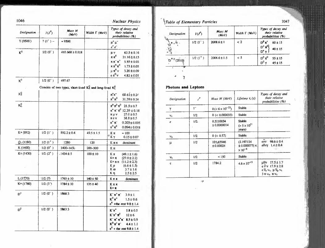
/(/> Mass M

(MeV)

7 0" ) - -9500

1/2 (O' ) 493.668 ±0.018

Width f (MeV) Types of decay and

their relative robabilities (%)

1/2(0') 497.67

Consists of two types, short-lived Ks and long-lived Kt

Ks JtV 68.61 ±0.24

s0*° 31.39±0.24

Ki> s0*0*0 21.5±0.7

s+ s' s® 12.39 ±0.18 spv 27.0 ±0.5 itev 38.8 ±0.5

s+s~ 0.203± 0.005

s°K? 0.094± 0.018

K* (892) 1/2 d' ) 892.2 ±0.4 49.5 ±1.5 Ks -100 *Ky 0.15±0.07

Gi (1280) 1/2(1*) 1280 120

K (1400) 1/2 (0* ) 1400-1450 200-300 KS

K« (1430) 1/2 (2+ ) 1434±5 !00±10 Ks (49.1 ±1.6) K* s (27.0 ±2.2) K* ss (11.2 ±2.3) Kp (6.6 ± 1.5) Kto 3.7 ±1.6 K1) 2.5 ±2.5

1/2(7) 1765 ±10 140± 50 K s s dominant

K* (1780) 1/2 (31 1784 ±10 135 ±40 K s s K* s

D+ 1/2 (O' ) 1868.3 K's+s' 3.9 ±1

K°s+ 1.5 ±0.6

e* +the rest 9.8 ±1.4

D° 1/2 (O' ) 1863.3 K's* 1.8 ±0.5

K's* S° 12 ±6

K's+sV 8.510.9

K° S+ S' 4.411.1

e* + the rest 9.8 ± 1.4

' Table of Elementary Particles

/(/) Mass M

(MeV)

1/2(1') 2008.611

1/2 (1* ) 2006.611.5

Width r (MeV)


probabilities (%)

Photons and Leptons

Designation Mass M (MeV) Lifetime t, (s)


probabilities (%)

p?V 17.5 ±1.7 e9v 17.9 ±2.8 ev,Vt, pv„vt 3*v,. «v.

. ..

. -

. .

Index

Accelerators classification 342 Cockroft-Valton generator 549 cyclic 554 electrostatic 548 in India 609 linear 601 pelletron 552

tendom 553 Van de Graff generator 551

Actinium series 69 Active deposits 71 Age determination

Libby’s method 467 of rocks and minerals 77

Alpha decay half-life 33 Alpha disintegration

energy 109

formation factor 109 hindrance factor 109 theory 100, 104

Alpha particles

charge determination 83, 86 Geigey’s law 99 long-range 111-112 mass 86 range 92

range-energy relation 97 specific charge 86 specific ionization 95

spectroscopic identification 89 stopping power 116 velocity 90

Alpha spectrum

fine structure 111 Alternating gradient focusing 588, 595

use of quadrupole magnets 593, 1015

Americanium (Z=95) 772

Angular correlation experiments 230

Angular distribution (of reaction prod¬ ucts) 513

Angular momentum

Clebach-Gordan coefficients 925, 1022

vector addition 1018 Anti-nucleons 919 Antineutrons 921 Antinuclei 921 Antiprotons 919

Betkelium (Z= 97) 774 Beta transformation

double decay 181 energetics 137

forms of interaction 162 inverse 184, 891 ’

parity non-conservation 172 selection rules 157, 159

Beta particles absorption 167

energy determination 131 energy distribution 132 ionisation loss 166 radiation loss 167 range 171

specific charge 126-128 Beta spectrometers 132

magnetic lens 135 resolving power 134

Beta spectrum 149

allowed and forbidden 151 comparative half-life 153 coulomb correction 148 deviations from Kurie plot 150 Fermi's theory 143 Kurie plot 150

Beta transitions (allowed and forbidden) 156

Betatron 567 energy limit 571

1048

.

1

oscillations 572 Binding fraction 21 Bubble chamber 277 Bucherer’s .experiment (e/m of P parti¬

cles) 128

Californium (Z = 98) 774 Charge independence 840 Charged particle spectroscopy 260 Charge symmetry 45 Cherenkov detedbr 267

theory 269 threshold type 271

Cloud chamber ' counter controlled 275, 970

diffusion type 276 expansion (Wilson) type 273-274

Coincidence counting 248 accidental coincidences 299 circuits 298 additive 299 anticoincidence circuits 301

Collective model of nuclei 412 coupling of particle and collective

motions 422 deformed nuclei 416

energy distribution 971 experimental methods 967 from extra galatic region 999 interactions 975 latitude effect 964 longitude effect 1025 nature of primaries 971 Rossi transition curve, 979 Variation belts 999-1000 shower 895 special techniques 886-887 Stormer’s theory 936

Coulomb corrections 148 Coulomb excitation 217 Cross section of scattering

differential 6, 190 total 6, 7

Curie 72 Curium (Z = 96) 773 Cyclotron 554

focusing of beam 558 ion sources 546 limitations 559 sector-focused 582 superconducting 585 synchro-cyclotron 560

rotational spectra 420 vibrational spectra 4l4

Collisions elastics 440 high energy 878 non-elastic 445

Compound nucleus hypothesis 487-490 Angular distribution 513-514 Breit-Winger formula 490 charged particle resonances 499 disintegration 507 entropy of residual nucleus 511 evaporation model 509 Ghoshal experiment 504 independence hypothesis 490 level density 511 resonances 495

Deuteron excited suite 793 ground state 785 magnetic moment 828 photo disintegration 830 quadrupole moment 827 radius 793-795 . wave equation 788 wave functions 792

Direct reactions 514 pick up 516 stripping 516

Direction focusing by electric field 318 by magnetic field 315 Double focusing principle 319

statistical model 502 second order 332

Conservation laws 911-919 Cosmic rays

absorption 878, 881 air showers 979 discovery 881 east-most asymmetry 957, 958,

965

Einsteinium (Z = 99) 775 Electron positron pair production 192 Electrometers

D.C feedback amplifiers 303 vacuum tube type 302 vibrating capacitance type 303

vibrating read type 322 Electron scattering experiment 26-28 Electroweak interaction 948

W and Z bosons 949 Weinberg Sal am model 950 neutral currents 951

Elementary particles Baryon 904 classification 904-933 hadrons 904 leptons 905 properties 906-910

Energy loss formula 113 ionisation loss 113

Fermium (Z = 100) 775 Focusing of charged particles

first order focusing 317 Form factor 28 Francium 784 Fusion process

critical temperature 759 cross section 750 Lawson criterion 761 pellet fusion 766 power released 757

Gamma rays Compton scattering 191 Dirac theory' 19$ electron positron annihilation

196 energy determination 197 gravitational ted shift 229 interaction in matter 188 Klein-Nishina formula J91 nuclear energy levels 202 pair creation 192 pair spectrometer 198 photoelectric absorption 188 positronium 196 scintillation spectrometer 199 Spectra and energy levels 202 Spectroscopy 261

Gamow Teliar Selection Rule 157 Geiger and Marsdon’s experiment 7, 8 Geiger-Muller counter 248

characteristics 250 efficiency 253 peateau 250 quenching 251

recovery time 252 Geiger-Nuttal law 99 Geiger region 246 Giant resonances 428 Grand unification theory 952

cosmological implications 953

Half-life of disintegration 55 for complex decay 76 measurement 73 of free neutron 170

Hadrons 904 baryons 904 mesons 905 properties 906-910

Heavy ion reactions 529 back bending 535 features 530 nuclear molecules 532 rotational spectra 534 super-heavy elements 533 techniques 529 transfer processes 534

Hyperons 894

discovery 894 properties 899, 901 A - hyperons 899 I - hyperons 899 S - hyperons 900 Q - hyperons 901 strangeneus 894

Inelastic scattering of electrons 218 Interactions

electromagnetic 901 electro-weak 903, 948 graviton 902 hyper-nuclei 903 strong nuclear 903 types 904 W and Z bosons 903, 949 weak nuclear 903-949

Internal conversion coefficient 213 Internal pair creation 216 Invariance

OPT theorem 915 change conjugation 913 coordinate inversion 911 hypercharge 920 spatial translation 913 time-reversal 915

1051

translation of time C09 violation of CP 916

tv Ion optics 315 A lonyfources 321, 543, 548

discharge type 544 '^jduoplasmatron 546

* electron impact type 321 electron oscillation type 544

* for cyclotrons 546 radiofrequency type 545

surface ionisation type 321 Ionic mobility 240

recombination 239 Ionisation

avalanches (Town send) 245 gas amplification 238 ionisation loss 120 primary 239 secondary 239

Ionisation chamber 239 integrating type 241 operation mode 241 pulse chamber 242 pulse size 242

Isobars 369 lsobaric analogue states 848 Isomeric (chemical shift) 228 Isospin 45. 409, 927 Isotones 16, 369 Isotopes 16

inventory of stable 368 Isotopic invariance 47

K-mesons 897 Decay modes 895-897 discovery 894 isospin 899 mean-lives 898 strangeness 896 t - 6 puzzle 896

If Lawrencium (Z= 103) 773 Leptons 143

interactions 905 lepton number 143, 891

Linear accelerator 601 accelerating system 609 focusing of beam 604 for heavy ions 608 phase focusing 605 power requirement 607

Mass defect 20 Mass dispersion 317 Mass measurement 314

double method 333 peak matching technique 338

Mass spectroscope Aston type 323 Bainbridge type 328 Bainbridge and Jordan type 331 Dempster type 322 double focusing type 319, 330 helical path type 335 mass synchrometer 336

Mattauch-Herzog type 331 omegatron 336 quadrupole type 339 resolving power 341 using cyclotron principle 334

Mesonic y-rays 30, 31 Mendeiesrium (Z * 101) 776 Microtron 579 Mirror nucleus 33, 161, 381

beta decay 381 Missing elements

synthesis of 782 Mossbauer effect (recoil - less transi¬

tion) 222-223 applications 227 chemical shift 228 gravitational red shift 229 hyperfine splitting 227

Muons decay 891 discoveiy 897 interactions 892 mass 901 atom 892 muonium 893 production 890 spin and magnetic moment 992

Neptunium series 68 Neutrino 139

antineutrino 180 detection 181 double beta decay 179 helicity 176-179 in muon decay 891 mass 151 properties 141, 892, 910

1052

Neutron age determination 667 age equation 665 charge 617 cross-section 639 decay 617 detectors 639 diffusion 653, 656 discovery 613 energy classification 620 log decrement 650 magnetic moment 618 mass 615 moderating ratio 651 monochromators 641 slowing down 647, 651 sources 621 spin 617

Neutron-proton capture 833 Neutron scattering 34

by neutrons 840

by ortho arid parahydrogen 815 elastic 474 effects of chemical finding 813 liquid mirror experiment 820

n-p scattering 813 cross-section 797 effective range theory 809-812 high energy 852 limits of energy 797 low energy 795 low energy parameters 821 partial wave method 796 phase shifts 798 reduced mass 813 r-

scattering length 800, 801 spin - dependence 806 wave functions 803

Nobelium, (Z = 102), 776 Non-central force 822

conservation rales 824-825 in deuteron 828 quadrapole moment 827 Rarita - Schwinger equation 825

Nuclear binding energy 15, 16 systematics 19

Nuclear charge determination (Chad- wide) 11, 1'4

Nuclear emulsion technique 281, 971 applications 285 particle identification 284

Index

range - energy relation 283 Nuclear fission

activation energy 681 asymmetry 675 Bohr-Wheeler theory 684 critical deformation energy 685 cross section 690 delayed neutrons 731 discovery 670 energetics 678 energy distribution 675 energy release 672 fertile materials 691 nature of fragments 674 neutron emission 676 pairing energy effect 683 quantum effect 689 saddle point 689 shape isomerism 693 spontaneous fission 678, 681 threshold 682

Nuclear force 840 effective range 809 exchange interaction 841 exchange operators 842, 846 generalized Pauli principle 847 isospin formalism 847 Meson theory 867 ordinary interaction 842 repulsive core 860 saturation 841 spin dependence 806 two nucleon potential 871

Nuclear fusion 695 carbon cycle 699 Lawson Criterion 760 proton - proton cycle 698 energy in stars 697

thermonuclear reactions 695 Nuclear isomerism 21 *

islands of isomerism 213, 404 shape isomerism 693 Nuclear magnetic moment 38,

400 atomic beam method 351 Bloch’s method 356 determination 351 electron paleo magnetic resonance

357

hyperfine splitting 341 microwave method 359

{ndex

nuclear induction method '358 Rabi’s magnetic resonance

method 352 \ resonance magnetic absorption *355

. Zeeman effect method 345 NufMhr mass 15

'determination 338 unit 18

Nuclear matrix element 160 Nuclear model ^

alpha decay 377 applications 377 Bdthe-W^eizsacker formula 372 configuration mixing 407 collective model 414 evaporation model 569 Fermi gas model 383 individual particle model 410 isomerism 404 liquid drop model 371 mass parabola 376 mirror nuclei 32. 381 optical model 520 quadrapole moment 406 Schmidt lines 403 shell model 407 single particle shell model 407 spin-orbit interaction 393 super fluid model 427 unified (Nilsson’s) model 424

Nuclear parity 37 Nuclear quadrapole moment 41, 43 Nuclear radius 24

charge radius 24, 27. 30. 33 mass radius 24 potential radius 32

Nuclear reactions a-induced 458 Cockroft-Walton experiment 451 compound nucleus model 487 conservation laws 436 cross section 455, 477, 479 deuteron-induced 463 direct reactions 514 discovery 433 endoergic 446 energetics 445 exoergic 449 y-induced 469 heavy-ion reactions 529

1053

life-time measurement 528 mechanisms 527 neutron induced 465 optical model 520 proton-induced 460 Q-value 449 types 435 yield 757

Nuclear reaction cross section 472 barrier penetration 499 detailed balance 477 limiting values 484 optical theorem 485 partial cross sections 455 partial wave method 479 reciprocity relation 479 shadow scattering 489 theory 472-477

Nuclear radiations biological effects 748 chemical effects 747 dosage 750 from accidents 753 from explosions 754 from waste disposal 754 hazards 750 physical effects 746 RBE 751 REM 752 REP 751

Nuclear reactors breeders 737, 738, 742 critical size 721 delayed neutrons 730 fast reactors 738, 739 gas cooled 743 heavy-water moderate (enriched

uranium) 734 ■«» Indian programme 744 mobile reactive 740 organic moderated 743 power reactors 740 production reactors 737 pulsed reactors 736 reaction shielding 729 reactor theory 717 research reactors 732, 744 uranium graphite (material) 733 water moderated 735, 740, 741

Nuclear reactor materials 725 cladding 728

1054 Index

control 728, 730 coolants 727 moderators 725 reflectors 726 structural materials 728

Nuclear spin 34 determination 341 from molecular spectra 348 hyperfine splitting 341 isotope effect 347 Pauli’s theory 36 Zeeman effect 345

Nuclear statistics 37, 348 Nucleo-synthesis

helium problem 705 E — process 703 P — process 704 R — process 704 S — process 703

Omegatron 336 Optical model 520

Weisskopt’s explanation 528 Orbital electron capture 163-164

theory 164

overlapping levels (Statistical model) 502

Packing fraction 20 Parity

conservation 914 C — 914 G —928 P — 915 ,r non-conservation (P-decay) 171 intrinsic 896, 922

Phase stability (principle) 563 in synchro-cyclotron 565 in synchrotron 576

Photomultiplier tubes 264 dynodes 265

Pi-mesons decay 885, 889 discovery 994 intrinsic parity 922 mass 887 neutril 887 production and properties 881 spin and parity 886

Plasma confinement magnetic method 762

magnetic mirror 765 stellarator 764 tokamak 762

Polarized nucleon scattering 861 Polonium 62 Pesitrons

annihilation 196 Dirac theory 193 discovery 197

Positronium 1% Proton-proton scattering

effect of nuclear force 836 high energies 858 low, energies 834

Principle of detailed balance 477 Promethium (Z = 61) 783 Proportional counter

neutron counting 244, 248 Pulse amplifiers 289

preamplifiers 291 Pulse counters 296

binary scalars 2% decade scalars 297

Pulse height analyzer multi channel (MCA) 295 single channel 294 Pulse shaping 287

Pulse size discriminators diode discriminator 293 Schmit trigger circuit 294

Quark bags 944 Quark hypothesis 938

baryon octet 941 beauty and truth 947 charmed quark 946 confinement 946 colours 944

experimental support 943 partons model 942 quantum chromo-dynamics 944 top or / quark 948

Quark structure baryons 940 masons 940

three quark combinations 940

Radiative transitions in nuclic 204 multipolarity 211 selection roles 208, 210 Welsekop’s formula 211

ftldex 1055

Radiative width measurement 233 Radioactive disintegration 51 S disintegration constant 55

displacement law 52 sucbtssive disintegrations 56

Radioactive radiations .^applications 755

tracer studies 755 Radioactive series 63

actinium-.series 69 equilibrium 56 nepturmium series 68 secular equilibrium 53 thorium iries 65, 68 transient equilibrium 51, 52 uranium-radium series 64, 65, 67

Radioactivity branching 69 discovery 49 growth and decay 52 induced 461 unit of 72

Radius (discovery) 62 Radon gas 71 Relative abundance of isotopes 16 Resonance fluorescene 216 Resonance particles 923

A - resonance 928 G - parity 928 mesonic resonances 929

Rogge resurrences 930 Rutherford’s nuclear model 10-11

Sargent diagram 159 Scattering

a-particles (Rutherford’s theory) 1

impact parameter 3, 4 interference 495 matrix 536 neutron 34 (f neutron-neutron 840 proton-proton 834 resonance 927

Scintillation detectors 262 counting arrangement 265 gamma detection 263 modes of energy transfer 262 pulse formation 267

Semiconductor detectors 254 depletion layer 7KA

diffused junction detectors 254 electron-hold pairs 254 Ge-Li detectors 258 HPGs detectors 258 Si—Li detectors 258 surface-barrier detectors 256 uses of 259 window thickness 257

Shell structure of nuclei 386 evidence 388 islands of isomerism 404 magnetic moment 394 nuclear spin 388 quadrupole moments 406 single particle states 389 spin-orbit interaction 393

Solid state track detectors 285 Spark chamber 279 Statistics of counting 304 Storage rings 597 Straggling of range 122 Strange particles 896 Strangeness conservation 918 Super-fluid model 427 Superheavy elements 781 Symmetry classification 933 SUz symmetry 933

SU3 symmetry 937 supermultiplets 937 weight diagrams 933

Synchrotron 575 electron 595 heavy-ion 596 phase stability 576 proton 585

Szilard Chalmers reaction 636

Technetium (Z = 43) 783 Thorium series 68 Transutanic elements 769

discovery 769 electronic configuration 780

Unified model 424 uranium-radium series 67

Voltage discrimination 292

Weak interaction 948

Zero-Zero transition 216

v--"' t W S.CHAND

Dear Readers, , J ! / j

S, Chand has always been at the forefront of Indian academic publishing. During its 70 years of service to the 'Knowledge Community’ in the country, the company has published close to unprecedented 7000 titles with support of its approximately coveted authors.

On its 70* anniversary, the company wishes not only to strengthen its relationship with its customers, but wishes to provide them best services and support befitting the knowledge economy of 21 “ century.

These efforts cannot be carried out in a generic manner and a proper segmentation of market to the ; customers has to be made in order to identify and service the needs of this particular group. This would

enable us to provide focused services and commitment to each category of our market segmentation by separately branding it. This would also provide a clear demarcation of different academic groups in the market both for the benefit of distributors, booksellers, libraries, students & teachers all alike.

The four separate colours have been identified to represent each segment of books as following:

• The Orange colour represents the School Books segment.

• The Green colour represents the Higher Academic Books segment,

e The Brown colour represents the Technical & Professional Books

• The Blue colour represents the Competition & Reference Books

These colours will be mark on the top & bottom of the spine of the book for easier identification.

SCHOOLBOOKS ■ZZT. This logo brings brightness of Sun, purity of fire, empowerment of light and fun of learning to «J|!^5* School Books. This logo lays down the foundation for a continuous learning for young iSSSP empowering minds for its voyage In the world of knowledge.

The logo of three solid blocks represents solidity, consolidation and the peak. This logo conveys the message to achieve greater and superior heights by using higher academic J books of S. Chand by its distinguished authors.

This logo represents technology in form of an electronic circuit highlighting the significance of technology and its constantly changing needs, continuously upgrades and revised technical books of S. Chand to meet the demands of Knowledge' & 'Industry'. *

COMPETITION AND REFERENCE BOOKS

The logo shows waves/bars that are converging towards a dot. The dot signifies "goar and the waves/bars denote “focus'' that is very much needed in preparation of Competitive Exams. The logo conveys the message that the competition and reference books by S. Chand will help the student to converge their attention towards their ambition.

S. Chand Management

A di vision of S, Chand & Company I ' !An ISO 9001 : 2000 Company)

7361. RAM fcAGAR. NEW DELHI-110 ■

i.com roup com

i

»

7

itiiiiiiii;

problems electric quadrupole moment

Documents