Moment Problems: old and new

Mihai Putinar

UCSB and NTU

November 26, 2013

Classical problem

Find a positive Borel measure µ on R, with prescribed moments

sk =

∫xkdµ(x), 0 ≤ k < n.

With n ≤ ∞.

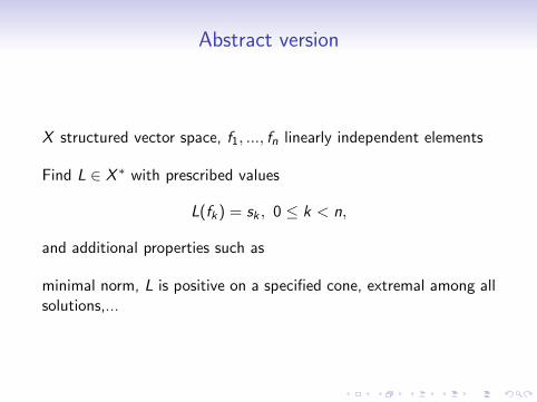
Abstract version

X structured vector space, f1, ..., fn linearly independent elements

Find L ∈ X ∗ with prescribed values

L(fk) = sk , 0 ≤ k < n,

and additional properties such as

minimal norm, L is positive on a specified cone, extremal among allsolutions,...

Statisticians first

M. G. Kendall: The Advanced Theory of Statistics, London, 1945.

In prectice numerical moments of order higher than fourth arerarely required, being so sensitive to sampling fluctuations thatvalues computed from moderate numbers of observations aresubject to a large margin of error.

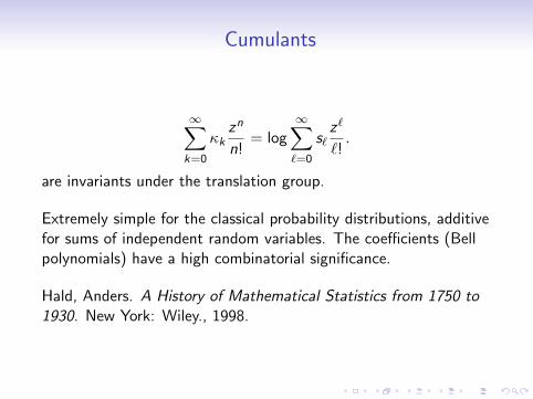
Cumulants

∞∑k=0

κkzn

n!= log

∞∑`=0

s`z`

`!.

are invariants under the translation group.

Extremely simple for the classical probability distributions, additivefor sums of independent random variables. The coefficients (Bellpolynomials) have a high combinatorial significance.

Hald, Anders. A History of Mathematical Statistics from 1750 to1930. New York: Wiley., 1998.

Best approximation

Chebyshev’s problem (around 1860):

Given a C 1-function F (x1, ..., xd ; p1, ...pn) on a domain Ω ⊂ Rd ,depending on parameters p1, ..., pn, find

minp1,...,pn

maxx1,...,xd

|F (x1, ..., xd ; p1, ...pn)|.

inspired by Poncelet’s extremal problem for p1x+p2√1+x2

− 1.

Both Chebyshev and A. A. Markov have extensively worked on thissubject, becoming masters of continued fractions, as a necessarytechnical tool.

Chebyshev polynomials

Consider the polynomial of minimal variation from zero, on aninterval [−h, h], of the form

f (x) = xn + p1xn−1 + . . .+ pn,

with p1, ..., pn parameters to be determined.

Necessarily

f (x)2 − L2 = (x2 − h2)f ′(x)2

n2

where L is the optimal value.

The division algorithm

f (x)−√

x2 − h2f ′(x)

n=

L2

f (x) +√

x2 − h2 f′(x)n

hence

1√x2 − h2

− f ′(x)

nf (x)=

L2

√x2 − h2f (x)[f (x) +

√x2 − h2f ′(x)/n

]

that is1√

x2 − h2− f ′(x)

nf (x)= O(

1

x2n+1).

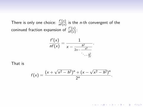
There is only one choice: f ′(x)nf (x) is the n-th convergent of the

coninued fraction expansion of f ′(x)nf (x) :

f ′(x)

nf (x)=

1

x − h2

2x− h2

...− h22x

.

That is

f (x) =(x +

√x2 − h2)n + (x −

√x2 − h2)n

2n.

Polynomial extrapolation

Chebyshev again

The real points x0, ..., xn,X are given. Knowing the approximativevalues of a polynomial F of degree n at n + 1 points xk , find theerrors in the values F (xk) which have minimal influence of thevalue F (X ).

As a matter of fact an extremal problem in square mean.

F (x) = µ0q0(x)f (x0) + . . .+ µmqn(x)f (xn)

with qk(x) unknown polynomials, such that

µ0qo(x)2 + . . .+ µnqn(x)2

is minimal.

Continued fractions

The solution exposed by Chebyshev reduces to a continued fractionargument. Given

n∑k=0

µkxk − z

= −s0z− s1

z2− . . .

find a polynomial P(x) of degree m such that

P(x)(s0z

+s1z2

+ . . .)

begins with a term of highest order.

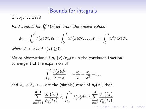
Bounds for integralsChebyshev 1833

Find bounds for∫ a0 f (x)dx, from the known values

s0 =

∫ A

0f (x)dx , s1 =

∫ A

0xf (x)dx , . . . , sn =

∫ A

0xnf (x)dx

where A > a and f (x) ≥ 0.

Major observation: if qm(x)/pm(x) is the continued fractionconvergent of the expansion of∫ A

0

f (x)dx

x − z= −s0

z− s1

z2− . . .

and λ1 < λ2 < ... are the (simple) zeros of pn(x), then

n−1∑k=`+1

qm(λk)

p′n(λk)<

∫ λn

λ`

f (x)dx <n∑

k=`

qm(λk)

p′n(λk)

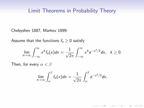
Limit Theorems in Probability Theory

Chebyshev 1887, Markov 1899:

Assume that the functions fn ≥ 0 satisfy

limn→∞

∫ ∞−∞

xk fn(x)dx =1√2π

∫ ∞−∞

xke−x2/2dx , k ≥ 0.

Then, for every α < β

limn→∞

∫ β

αfn(x)dx =

1√2π

∫ β

αe−x

2/2dx .

Stieltjes memoir, 1894-95

The sequence (sk)∞k=0 represents the moments of a positivemeasure supported on [0,∞) if and only if the continued fractionexpansion

s0z

+s1z2

+ . . . =1

c0z − 1c1− 1

c2z−1

c3−...

contains only non-negative terms ck ≥ 0.

DeterminatenessIf∑∞

k=0 ck =∞, then the convergents Pm(z)Qm(z)

converge in the

upper-half plane to∫∞0

dσ(x)z−x , and the measure σ ≥ 0 is unique.

If∑∞

k=0 ck <∞, then the convergents satisfy in the upper-halfplane:

P2k(z)→ p(z), Q2k(z)→ q(z),

P2k+1(z)→ p1(z), Q2k+1(z)→ q1(z),

where p, q, p1, q1 are entire functions of genus zero, satisfying

q(z)p1(z)− q1(z)p(z) = 1.

In that case the problem has infinitely many solutions, with distinctCauchy transforms. Among these:

p(z)

q(z)=∞∑k=1

µkz − λk

,p1(z)

q1(z)=∞∑k=1

µ′kz − λ′k

.

More on continued fractions

Hamburger 1919-1921

solves the power moment problem on the real axis, remarking(following Stieltjes) the positivity of the Hankel determinants

det

s0 s1 . . . sns1 s2 . . . sn+1...

. . ....

sn sn+1 . . . s2n

≥ 0

as necessary and sufficient conditions for solvability.

Recent references

Iosifescu, Kraaikamp: Metrical Theory of Continued Fractions,Springer 2002Cuyt, Brevik Petersen, Verdonk, Waadeland, Jones: Handbook ofContinued Fractions, Springer 2008Khrushchev: Orthogonal Polynomials and Continued Fractions,Cambridge U. Press, 2008.

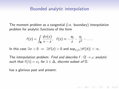
Bounded analytic interpolation

The moment problem as a tangential (i.e. boundary) interpolationproblem for analytic functions of the form

f (z) =

∫R

dσ(x)

x − z, f (z) ≈ −s0

z− s1

z2− . . . .

In this case =z > 0 ⇒ =f (z) > 0 and supt≥1 |tf (it)| <∞.

The interpolation problem: Find and describe f : Ω→ ω analyticsuch that f (λ) = cλ for λ ∈ ∆, discrete subset of Ω.

has a glorious past and present:

Google citations, Nov. 2013

Caratheodory-Fejer interpolation 10,200Nevanlinna-Pick interpolation 29,500Schur algorithm 407,000H∞-control 7,160,000

Nevanlinna parametrization

Obtained around 1922 by Hamburger and Nevanlinna:free parametrization of all solutions to the power momentproblem, in the indeterminate case

f (z) =

∫R

dσ(x)

x − z= −p(z)φ(z)− p1(z)

q(z)φ(z)− q1(z),

where φ(z) is any analytic function satisfying =φ(z) ≥ 0 whenever=z > 0.

Berg: Indeterminate moment problems and the theory of entirefunctions, J. Comput. Appl. Math. 65: 13(1995), 27 - 55.

Fourier transform

Known as the method of characteristic function in Probability

σ(ξ) =1√2π

∫ ∞−∞

e−ixξdσ(x)

uniquely determines σ (by known inversion formulae).

Bochner: σ ≥ 0 if and only if σ(ξ1 − ξ2) is a positive semi-definitekernel.

If the moments exist σ ∈ C∞ and

sk =√

2π(−i)k σ(k)(0), k ≥ 0.

Carleman’s approach

Quasi-analytic Functions (1926):

u ∈ C∞[0, 1] is fully determined by (u(k))∞k=0 if and only if

∞∑k=0

1

Lk=∞

where|u(k)(x)| ≤ K k+1Mk , 0 ≤ x ≤ 1, k ≥ 0,

andLk = inf

j≥kM

1/jj .

Determinateness

via quasi-analyticity

∞∑k=0

1

s1/(2k)2k

=∞

implies uniqueness of the positive measure on R with moments(sk).

∞∑k=0

1

s1/(2k)k

=∞

implies uniqueness of the positive measure on [0,∞) withmoments (sk).

Reconstruction

Carleman’s reconstruction formula of a quasi-analytic functionu ∈ C∞M :

u(x) = limn→∞

n−1∑k=0

ωn,ku(k)(0)xk ,

where the coefficients ωn,k depend only on the class C∞M .

Laplace transform

g(t) = L(σ)(t) =

∫ ∞0

e−xtdσ(x),

also satisfiessk = (−1)kL(σ)(k)(0), k ≥ 0

whenever the moments exist.Analytic extension

L(σ)(z) =

∫ ∞0

e−xzdσ(x),

for Rez > 0 with known inversion formulae...

S. Bernstein (1929): characterization of transforms of positivemeasures

g ∈ C∞[0,∞), (−1)kg (k) ≥ 0, k ≥ 0.

Abolutely continuous measures

dσ(x) = τ(x)dx , τ ∈ Lp([0,∞))

has Laplace transform in a Hardy class of the right half-plane, withan arsenal of function theory of a complex variable available.

Widder (1934) inversion: g(t) = L(τdx)(t) reads

limk→∞

(−1)kg (k)(k

t)(

k

t)k+1 = τ(t), t > 0.

Summation of divergent series

Improving the convergence of series by average methods, inducedby a regular summation scheme

tn =n∑

k=0

ankuk ,

so thatlim un = u ⇒ lim tn = u.

Hausdorff (1921) A sequence (sn)∞n=0 represents the moments of aprobability measure on [0, 1] if and only if the matrixDdiag(s0, s1, ...)D induces a regular summation scheme, where

D = ((−1)n(

kn

)).

Extension of linear functionals

A positive Borel measure σ on R, admitting all moments, is givenby a positive linear functional L : Cp(R) −→ R, where Cp is thespace of continuous functions of polynomial growth:∫

fdσ = L(f ), f ∈ Cp(R).

M. Riesz (1922-23) Solving the moment problem by linearextension of positive linear functionals

Ld : Rd [x ] −→ R

whereRd [x ] = p ∈ R[x ]; deg p ≤ d.

Convexity

M. Riesz method prompted to study the convex cones

p ∈ Rd [x ], p(x) ≥ 0, x ∈ K

and

σ ∈ M+(R),

∫xkdσ(x) = sk , 0 ≤ k ≤ n.

Caratheodory (1911) carried earlier a similar analysis on the unitcircle T.

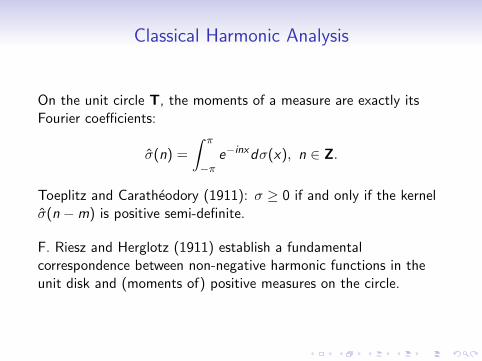
Classical Harmonic Analysis

On the unit circle T, the moments of a measure are exactly itsFourier coefficients:

σ(n) =

∫ π

−πe−inxdσ(x), n ∈ Z.

Toeplitz and Caratheodory (1911): σ ≥ 0 if and only if the kernelσ(n −m) is positive semi-definite.

F. Riesz and Herglotz (1911) establish a fundamentalcorrespondence between non-negative harmonic functions in theunit disk and (moments of) positive measures on the circle.

Hilbert space

The moments of a positive measure σ are structured in anon-negative definite Gramm matrix

sk+m =

∫xkxmdσ(x) = 〈xk , xm〉2,σ.

Hence an associated system of orthogonal polynomials

Pk(x) = γkzk + O(zk−1), 〈Pk ,Pm〉2,σ = δkm.

The leading coefficient solves an extremal problem, a laChebyshev-Markov:

γ−1k = infdeg q≤k−1

‖zk − q(z)‖2,σ.

Christoffel functionsGiven orthonormal polynomials Pn, the Christoffel function

Cn(z , z) =n∑

k=0

|Pk(z)|2

and its polarization

Cn(z ,w) =n∑

k=0

Pk(z)Pk(w)

are essential in the study of the asymptotics of the polynomials Pn.

M. Riesz (1923): the solution to the extremal problem

ρn(λ) = min‖q‖22,σ, deg q ≤ n, q(λ) = 1

is attained by the polynomial

ρn(z) =C (z , λ)

C (λ, λ).

Weyl circle

Another parametrization of all solutions, obtained via the values ofthe Cauchy transforms

C (σn)(λ) =

∫dσn(x)

x − λ,

∫xkdσn(x) = sk , k ≤ n.

They form a disk of radius ρn.

Parallel theory to the continuous case (Sturm-Liouville problem)studied by H. Weyl a decade before Riesz.

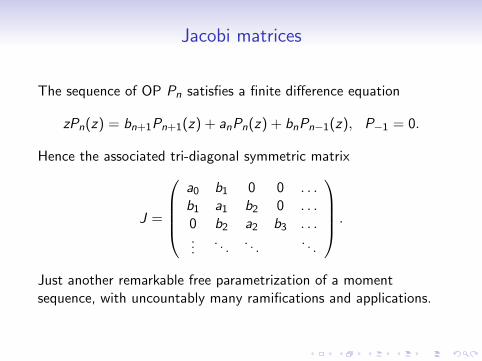
Jacobi matrices

The sequence of OP Pn satisfies a finite difference equation

zPn(z) = bn+1Pn+1(z) + anPn(z) + bnPn−1(z), P−1 = 0.

Hence the associated tri-diagonal symmetric matrix

J =

a0 b1 0 0 . . .b1 a1 b2 0 . . .0 b2 a2 b3 . . ....

. . .. . .

. . .

.

Just another remarkable free parametrization of a momentsequence, with uncountably many ramifications and applications.

OP literature

Herbert Stahl, Vilmos Totik: General orthogonal polynomials,Encyclopedia of Mathematics and its Applications, 43 CambridgeUniversity Press, Cambridge, 1992. xii+250 pp.

Barry Simon: Orthogonal poynomials on the unit circle, 2. vol.,Amer. Math. Soc. 2004.

The Oxford Handbook of Random Matrix Theory (OxfordHandbooks in Mathematics), (G. Akemann et al, eds.), OxfordUniv. Press, 2011.

Google citations (Nov. 2013):OP 2,690,000RM 17,000,000

The spectral theoremHilbert, Hellinger, Hahn, F. Riesz (around 1910)Let U be a unitary transformation on a Hilbert space and let ξ bea fixed vector. The sequence 〈Unξ, ξ〉, n ∈ Z is represented by apositive measure µ on the unit circle, because the kernel

sk−m = 〈Ukξ,Umξ〉

is positive semi-definite. Hence

〈q(U)ξ, ξ〉 =

∫ π

−πq(e it)dµ(t), q ∈ C[x ].

With the known techniques of integration theory, one can definef (U) for any bounded Borel function, so that

〈f (U)ξ, ξ〉 =

∫ π

−πf (e it)dµ(t).

Similarly

Given a bounded symmetric linear operator S , densely defined on aHilbert space, and a vector ξ, the sequence

sk = 〈Skξ, ξ〉, k ≥ 0

is a moment sequence, because the kernel sk+m = 〈Skξ,Smξ〉 ispositive semi-definite. Therefore there exists a positive measureon the line, such that

〈f (A)ξ, ξ〉 =

∫f (x)dσ(x),

for every bounded Borel function on the line.

Self-adjointnessvon Neumann (1929), Stone (1930)

The case of a symmetric linear operator S , densely defined butunbounded: even when all powers Snξ are well defined andsk+m = 〈Skξ,Smξ〉 is a moment sequence, the Borel functionalcalculus f (S) may exist only on a larger Hilbert space. Theself-adjoint condition

S = S∗

is necessary for having a spectral theorem/decomposition in theoriginal Hilbert space.

Since then, this is the natural theoretical framework for quantummechanics.M. H. Stone: Linear transformation in Hilbert space, Amer. Math.Soc., 1932.B. Simon: The classical moment problem as a self-adjoint finitedifference operator, Adv. Math. , 137 (1998) pp. 82203.

Mark G. Krein (1907-1989)Has incorporated the classical problem of moments in modernanalysis, with great, original contributions. Master of the geometryof Hilbert space and function theory of a complex variable. A fewof his topics of research:

Strings and spectral functionsSelf-adjoint operators on Hilbert spaces of entire functionsExtremal problems related to the truncated moment problemConvex analysis and dualityPrediction theory of stochastic processesStability and control of systems of differential equationsRepresentation theory of locally compact groupsSpectral analysis in spaces with an indefinite metric

Had 50 students, 805 descendants (many working today onmoment problems) and was the uncontested mentor of theUkrainian school of Functional Analysis.

Moment method in numerical mathematics

Given f0, ..., fn linearly independent vectors in a Hilbert space,analyse the linear transformation An : Hn −→ Hn such that

Anfk = πnfk+1, 0 ≤ k ≤ n − 1,

where Hn = lin.span(f0, ..., fn−1) and πn is the orthogonalprojection onto Hn.

Yu. V. Vorobiov, The method of moments in applied mathematics,Fizmatgiz, Moscow, 1958.Roger F. Harrington, Field Computation by Moment Methods,Wiley 1993.L. Trefethen, M. Embree: Spectra and pseudospectra, Princeton,2005.

Multivariate moments

Around for a century or so, still intriguing and occupying therecent generations. Challenges:

Algebraic structure of positive polynomialsConvex analysis of moment dataMatrix completion and extension of linear functionalsFunction theory of several complex variablesCommuting systems of symmetric linear operatosDeterminateness

Some recent applications and ramifications

Global polynomial optimizationGeometric tomographyBolzmann equations and max. entropySignal processing via wavelet transformsElliptic growthFree probability theory

Free cumulants

”...free independence can be characterized by the vanishing ofmixed cumulants. An important technical tool for deriving thischaracterization is a formula for free cumulants where thearguments are products of random variables. This formula isactually at the basis of many of our forthcoming results in laterlectures and allows elegant proofs of many statements.”

A. Nica, R. Speicher: Lectures on the Combinatorics of FreeProbability, Cambridge Univ. Press, 2006.