problem book for 2008 - 2009, available from actsci course office
TRANSCRIPT
Operational Research
Module AS3021
Problem Book
Dr G BowtellCity University
Contents
A Worksheets 1A.1 Worksheet 1 . . . . . . . . . . . . . . . . . . . . . . . . . . . . . . . . . . . . . . . . . . 1A.2 Worksheet 1 - Solutions . . . . . . . . . . . . . . . . . . . . . . . . . . . . . . . . . . . 3A.3 Worksheet 2 . . . . . . . . . . . . . . . . . . . . . . . . . . . . . . . . . . . . . . . . . . 9A.4 Worksheet 2 - Solution . . . . . . . . . . . . . . . . . . . . . . . . . . . . . . . . . . . . 10A.5 Worksheet 3 . . . . . . . . . . . . . . . . . . . . . . . . . . . . . . . . . . . . . . . . . . 14A.6 Worksheet 3 - Solutions . . . . . . . . . . . . . . . . . . . . . . . . . . . . . . . . . . . 15A.7 Worksheet 4 . . . . . . . . . . . . . . . . . . . . . . . . . . . . . . . . . . . . . . . . . . 18A.8 Worksheet 4 - Solutions . . . . . . . . . . . . . . . . . . . . . . . . . . . . . . . . . . . 19A.9 Worksheet 5 . . . . . . . . . . . . . . . . . . . . . . . . . . . . . . . . . . . . . . . . . 25A.10 Worksheet 5 - Solutions . . . . . . . . . . . . . . . . . . . . . . . . . . . . . . . . . . . 27A.11 Worksheet 6 - Class Example - No solution given . . . . . . . . . . . . . . . . . . . . . 33
B Past Exam - May 2008 35B.1 Question Paper . . . . . . . . . . . . . . . . . . . . . . . . . . . . . . . . . . . . . . . . 35B.2 Solutions . . . . . . . . . . . . . . . . . . . . . . . . . . . . . . . . . . . . . . . . . . . 44
C Past Exam - May 2007 55C.1 Question Paper . . . . . . . . . . . . . . . . . . . . . . . . . . . . . . . . . . . . . . . . 55C.2 Solutions . . . . . . . . . . . . . . . . . . . . . . . . . . . . . . . . . . . . . . . . . . . 63
D Past Exam - May 2006 73D.1 Question Paper . . . . . . . . . . . . . . . . . . . . . . . . . . . . . . . . . . . . . . . . 73D.2 Solutions . . . . . . . . . . . . . . . . . . . . . . . . . . . . . . . . . . . . . . . . . . . 80
E Specimen Exam Type Questions and Solutions 91E.1 Specimen Questions . . . . . . . . . . . . . . . . . . . . . . . . . . . . . . . . . . . . . 91
E.1.1 Minimal spanning tree problem . . . . . . . . . . . . . . . . . . . . . . . . . . . 91E.1.2 Shortest distance problem . . . . . . . . . . . . . . . . . . . . . . . . . . . . . . 92E.1.3 Maximum Flow - Minimum Cut - Ford-Fulkerson . . . . . . . . . . . . . . . . . 94E.1.4 Dynamic Programming . . . . . . . . . . . . . . . . . . . . . . . . . . . . . . . 95E.1.5 Linear Programming . . . . . . . . . . . . . . . . . . . . . . . . . . . . . . . . . 98
E.2 Solutions . . . . . . . . . . . . . . . . . . . . . . . . . . . . . . . . . . . . . . . . . . . 102
i
CONTENTS ii
F Specimen Courseworks 116F.1 Coursework 1 - 2007 . . . . . . . . . . . . . . . . . . . . . . . . . . . . . . . . . . . . . 116F.2 Coursework 1 - 2007 Solution . . . . . . . . . . . . . . . . . . . . . . . . . . . . . . . . 118F.3 Coursework 2 - 2007 . . . . . . . . . . . . . . . . . . . . . . . . . . . . . . . . . . . . . 123F.4 Coursework 2 - 2007 Solution . . . . . . . . . . . . . . . . . . . . . . . . . . . . . . . . 123F.5 Coursework 1 - 2008 . . . . . . . . . . . . . . . . . . . . . . . . . . . . . . . . . . . . . 127F.6 Coursework 1 - 2008 Solutions . . . . . . . . . . . . . . . . . . . . . . . . . . . . . . . . 130F.7 Coursework 2 - 2008 . . . . . . . . . . . . . . . . . . . . . . . . . . . . . . . . . . . . . 133F.8 Coursework 2 - 2008 Solutions . . . . . . . . . . . . . . . . . . . . . . . . . . . . . . . . 135

Appendix A
Worksheets
A.1 Worksheet 1
1. Inequalities
Graphically display the feasible region defined by the following inequalities:
2x1 + 2x2 ≤ 8 3x1 + 2x2 ≤ 12 x1 + 0.5x2 ≤ 3 x1 ≥ 0, x2 ≥ 0
Maximize z = 3x1 + 2x2 on the feasible region. Which, if any, of the first three inequalities maybe removed without affecting the optimum solution?
2. Inequalities
Consider the following linear programming model:
Maximize the objective function z = 3x1 + 3x2 subject to the constraints:
2x1 + 4x2 ≤ 12 6x1 + 4x2 ≤ 24 x1 ≥ 0, x2 ≥ 0
(a) Find the optimal solution using graphical means.
(b) If the objective function is changed to z = 2x1 + 6x2 what will the optimum solution be.
3. Workload Balancing
The company Snap produces photo printers for both the professional and consumer markets.The Snap consumer division recently introduced two photo printers that provide colour printsrivaling those produced by a professional processing lab. The P100 model can produce a 100mm× 150mm borderless print in 40 seconds. The more sophisticated and faster P150 can evenproduce a 300mm× 500mm print. Financial projections show profit contributions of £42 foreach P100 and £87 for each P150.
The printers are assembled, tested and packaged at Snap’s plant located in New Barnet. Thisplant is highly automated and uses two manufacturing lines to produce the printers. Line 1performs the assemble operation with times of 3 mins per P100 printer and 6 mins per P150printer. Line 2 performs both the testing and packaging operations. Times are 4 mins per P100
1

APPENDIX A. WORKSHEETS 2
printer and 2 mins per P150 printer. The shorter time for the P150 is a result of its faster printspeed. Both manufacturing lines are in operation for one 8-hour shift per day.
The problem
Perform an analysis for Snap by consider the following points.
(a) Obtain the best number of units of each type to produce in order to maximize the totalcontribution to profit in an 8 hour shift. What reasons might management have for notimplementing your recommendation?
(b) Suppose that management also states that the number of P100 printers produced shouldbe at least as great as the number of P150 produced? Again assuming that the objectiveis to maximize the total contribution to profit in an 8 hour shift, how many units of eachprinter should be produced?
(c) Does the solution you have in (b) balance the total time spent on Line 1 with that on Line2? Why should this be of concern to management?
(d) Management requested an expansion of the model in (b) that would produce a betterbalance between the total time on Line 1 and that on Line 2. They want to limit thedifference between the time spent on the two lines in the 8-hour shift to be no more than30mins. If the objective is still to maximize the total profit how many units of each printershould be produced? What effect does this work-load balance have on the total profit in(b)?
(e) Suppose that in part (a) management specified the objective as maximizing the total numberof printers produced each shift rather than the total profit contribution. With this objective,how many units of each printer should be produced per shift? What effect does thisobjective have on total profit and workload balance?
4. Production Strategy
Fit-Fit manufactures exercise equipment at its plant in York. It recently designed two universalweight machines for the home exercise market. Both machines use Fit-Fit’s patented technologythat provides the user with an extremely wide range of motion capabilities for each type ofexercise performed. Until now, such capabilities have been available only on expensive weightmachines used primarily by physical therapists.
At a recent trade show, demonstrations of the machines resulted in significant dealer interest.In fact, the number of orders that Fit-Fit received at the trade show far exceeded its manu-facturing capabilities for the current production period. As a result, management decided tobegin production of the two machines. The two machines, which Fit-Fit named Body-Firm andBody-Strong, require different amounts of resource to produce.
Body-Firm consists of a frame unit, a press station and a pec-dec station. Each frame produceduses four hours of machining and welding time and two hours of painting and finishing time.Each press station requires two hours of machining and welding and one hour of painting andfinishing, and each pec-dec station uses two hours of machining and welding time and two hours

APPENDIX A. WORKSHEETS 3
of painting and finishing time. In addition two hours are spent assembling, testing and packagingeach Body-Firm unit. The raw material costs £450 for each frame, £300 for each press stationand £250 for each pec-dec station. Packaging costs are estimated at £50 per unit.
Body-Strong consists of a frame unit, a press station, a pec-dec station, and a leg press station.Each frame produced uses five hours of machining and welding time and four hours of paintingand finishing time. Each press station requires three hours machining and welding time andtwo hours of painting and finishing time, each pec-dec station uses two hours of machining andwelding time and two hours of painting and finishing time, and each leg press station requirestwo hours of machining and welding time and two hours of painting and finishing time. Inaddition, two hours are spent assembling, testing, and packaging each Body-Strong unit. Theraw material costs are: £650 for each frame, £400 for each press station, £250 for each pec-decstation, and £200 for each leg press station; packaging costs are estimated to be £75 per unit.
For the next production period, management estimates that 600 hours of machining and weldingtime, 450 hours of painting and finishing time, and 140 of assembly, testing, and packaging timewill be available. Current labour costs are £20 per hour for machining and welding time, £15per hour for painting and finishging time, and £12 per hour for assembly, testing, and packagingtime. The market in which the two machines must compete suggests a retail price of £2,400for the Body-Firm unit and £3,500 for the Body-Strong unit, although some flexibility may beavailable to Fit-Fit because of the unique capabilities of the new machines. Authorised Fit-Fitdealers can purchase machines for 70% of the suggested retail price.
Fit-Fit’s President believes that the unique capabilities of the Body-Strong unit can help positionFit-Fit as one of the leaders in high-end exercise equipment. Consequently, he has stated thatthe number of units of Body-Strong produced must be at least 25% of the total production.
The problem
Analyse the production strategy at Fit-Fit as follows:
(a) What is the recommend number of Body-Firm and Body-Strong machines to produce inorder to maximize profit.
(b) How does the requirement that the number of units of Body-Strong produced be at least25% of the total production affect profits?
(c) Where should efforts be expended to increase profits?
A.2 Worksheet 1 - Solutions
1. In Fig. A.1(a) the feasible region is shown hashed. As 3x1 + 2x2 = 12 does not form part of theboundary of the feasible region the constraint 3x1 +2x2 ≤ 12 is redundant and may be removedwithout affecting the feasible region.
The objective function has been plotted with z = 6. As this value of z is increased the objectivefunction moves away from the origin and last intersects the feasible region at P . The point P
therefore is the point at which z attains its maximum.

APPENDIX A. WORKSHEETS 4
As P lies on the intersection of 3 = x1 +0.5x2 and 8 = 2x1 +2x2 the coordinates of P are (2, 2).Hence the maximum value of z is z = 3(2) + 2(2) = 10.
2. (a) In Fig. A.1(b) the feasible region is shown hashed. The objective function z = 3x1 + 3x2
is shown plotted with z = 6. As z increases this moves away from the origin and lastintersects the feasible region at B. Calculating the coordinates of B from the intersectionof 6x1 + 4x2 = 24 and 2x1 + 4x2 = 12 gives B(3, 1.5) and hence the maximum value ofz = 3(3) + 3(1.5) = 13.5.
(b) In Fig. A.1(b) the objective function z = 2x1 + 6x2 is shown plotted with z = 12. As z
increases this moves away from the origin and last intersects the feasible region at A whichhas coordinates (0, 3), hence the maximum value of z = 2(0) + 6(3) = 18.
5 5
5 5
x1 x1
x2 x2
.....................................
3x1 + 2x2 = 12(redundant)
z = 6 = 3x1 + 2x2
7
x1 + 0.5x2 = 3
2x1 + 2x2 = 8
7 7
(a) (b)
P ................................................................
..............................
6x1 + 4x2 = 24
2x1 + 4x2 = 12
z = 6 = 3x1 + 3x2
z = 12 = 2x1 + 6x2
µ µ
A
B
Figure A.1: Feasible regions hashed. Objective functions dotted (a) z = 10 max at P (2, 2)(b) z = 2x1 + 6x2 max at A(0, 3), value 18. z = 3x1 + 3x2 max at B(3, 1.5), value 13.5.
3.
Identify the problem
In this problem the questions to be addressed are listed, however if the problem was just ’inves-tigate’ then a list of such questions would need to be constructed.
A good starting point to try and understand any problem is to collect together the data, in thiscase in the form of a table, as follows:
Formulate the model

APPENDIX A. WORKSHEETS 5
Type Line 1 Line 2 ProfitP100 3 4 £42P150 6 2 £87
Available 480 480time
Table A.1: Processing times in minutes per item and profit in £ per item. Total of 480min processingtime available for each type
Let p1 and p2 denote the number of P100 and P150 printers produced in a given shift.
The problem will involve maximizing the profit which is given by z = 42p1 + 87p2.
The constraints due to the limitation of production time on each line are:
3p1 + 6p2 ≤ 480, 4p1 + 2p2 ≤ 480 p1, p2 ≥ 0 (A.1)
Carry out Mathematics
(a) The feasible region given by the inequalities in Eq(A.1) is shown in the graph in FigureA.2(a). The objective function is shown with z = 3654 = 42p1 + 87p2. Since it is not clearwhether z is max at A or B we can either evaluate z at these points or compare the gradientof AB with that of z.
Coordinates of A are (106 23 , 26 2
3) and give z = 6800.
Coordinates of B are (0, 80) and give z = 6960.
Hence the recommendation is to produce eighty P150 in the eight hour shift and none ofthe P100 model. This gives a profit of £6960. This may not be acceptable since it is notgood marketing strategy to only have one product.
(b) For the additional constraint p1 ≥ p2 the new feasible region is show in Figure A.2(b). It isclear in this case that the objective function is maximum at C. The coordinates of C are(53 1
3 , 53 13) and at this point z = 6880
Thus if the company is to produce at least as many P100 models as P150 then they shouldproduce 53 units of each. This will give a little slack in the system and will lead to a profitof £6837.(no rounding analysis carried out)
(c) The production time for line 1 is 3p1 + 6p2 which with p1 = p2 = 53 gives 477mins. Theexact value at C giving 480 which is binding. The production time for line 2 is 4p1 + 2p2
which p1 = p2 = 53 gives 318 mins , showing a considerable amount of slack on this line.(this doesn’t improve much if we use the exact values from the coordinates of C).
Clearly therefore the production lines are not balanced and this will lead to idle labourwhich cannot be considered as a good thing.
(d) The idea of a fully occupied workforce and the production of both types of product arenow to be thought more important than just theoretically making a maximum profit. Ahappy workforce and long term sales are obviously important. To this aim the company

APPENDIX A. WORKSHEETS 6
12
16
8
24
..................
..................
................
B
A
¸
z = 3654 = 42p1 + 87p2
3p1 + 6p2 = 480
4p1 + 2p2 = 480
(a)
p1
p2
12
16
8
24
..................
..................
................
C
p1 = p2
B
A
¸
z = 3654 = 42p1 + 87p2
3p1 + 6p2 = 480
4p1 + 2p2 = 480
(b)
p1
p2
Figure A.2: Scale on both axes 1:10
now imposes a constraint so that there is no more than 30min difference between the twoproduction lines.Thus the additional constraint is
|(3p1 + 6p2)− (4p1 + 2p2)| ≤ 30 ⇒ |4p2 − p1| ≤ 30 ⇒ −30 ≤ 4p2 − p1 ≤ 30
Thus the feasible region has to also lie between the lines −30 = 4p2− p1 and 4p2− p1 = 30.This is shown in Figure A.3(a)The objective function is now maximum at T which has coordinates (96 2
3 , 31 23) which gives
z = 6815 Without doing any rounding analysis we could suggest they produced 96 P100and 31 P150 to satisfy the added requirements.
(e) Figure A.3(b) is simply Figure A.2(a) with a different objective line. It is clear that themaximum now occurs at A. The coordinates of A are (106 2
3 , 26 23) and the corresponding
value of z is £6800.Since A lies on both the bounding lines for the availability of time on the two lines theconstraints are binding. Thus the two lines have no slack and hence in balance.
4.
Identify the problem
Again the problem states quite specifically which questions to address. However the problemhas a lot data associated with it, this is best extracted and displayed by forming tables.

APPENDIX A. WORKSHEETS 7
12
16
8
24
..................
..................
...............
C
p1 = p2
B
A
>
z = 3654 = 42p1 + 87p2
3p1 + 6p2 = 480
4p1 + 2p2 = 480
(a)
p1
p2
T
4p2 − p1 = −30
4p2 − p1 = 30
12
16
8
24
z = 80 = p1 + p2
B
A
3p1 + 6p2 = 480
4p1 + 2p2 = 480
(b)
p1
p2
Figure A.3: Scale on both axes 1:10
Body-Firm Frame Press Pec-Dec TotalMach/Weld(hr) 4 2 2 8Paint/Fin(hr) 2 1 2 5
Ass/Test/Pk(hr) - - - 2Cost(£) 450 300 250 1000+pk=1050
Table A.2: Construction time and costs for the Body-Firm equipment. Packaging (pk) £50/item
Formulate the model
Let F and S be the number of Body-Firm and Body-Strong pieces of equipment produced. Usingthe data from Table A.2, TableA.3 and Table A.4 for the amount of resource used to produceeach item and the amount of resource available we can write down the following constraints:
8F + 12S ≤ 600 5F + 10S ≤ 450 2F + 2S ≤ 140 F, S ≥ 0 (A.2)
The profit function is the difference of the cost and the revenue. Bearing in mind that thecompany only gets 70% of the RRP the revenue from selling F and S is given by:
Revenue = 2700× 70%× F + 3500× 70%× S = 1680F + 2450S
The cost of material plus packaging is given by 1050F + 1575S and the cost of labour in thethree construction areas is given by:
Labour Cost = (8F + 12S)20 + (5F + 10S)15 + (2F + 2S)12 = 259F + 414S
APPENDIX A. WORKSHEETS 8
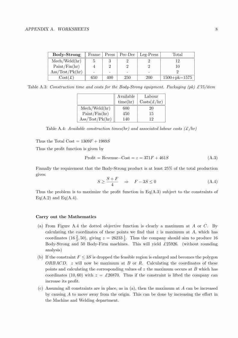
Body-Strong Frame Press Pec-Dec Leg-Press TotalMech/Weld(hr) 5 3 2 2 12Paint/Fin(hr) 4 2 2 2 10
Ass/Test/Pk(hr) - - - - 2Cost(£) 650 400 250 200 1500+pk=1575
Table A.3: Construction time and costs for the Body-Strong equipment. Packaging (pk) £75/item
Available Labourtime(hr) Costs(£/hr)
Mech/Weld(hr) 600 20Paint/Fin(hr) 450 15
Ass/Test/Pk(hr) 140 12
Table A.4: Available construction times(hr) and associated labour costs (£/hr)
Thus the Total Cost = 1309F + 1989S
Thus the profit function is given by
Profit = Revenue−Cost = z = 371F + 461S (A.3)
Finnally the requirement that the Body-Strong product is at least 25% of the total productiongives:
S ≥ S + F
4⇒ F − 3S ≤ 0 (A.4)
Thus the problem is to maximize the profit function in Eq(A.3) subject to the constraints ofEq(A.2) and Eq(A.4).
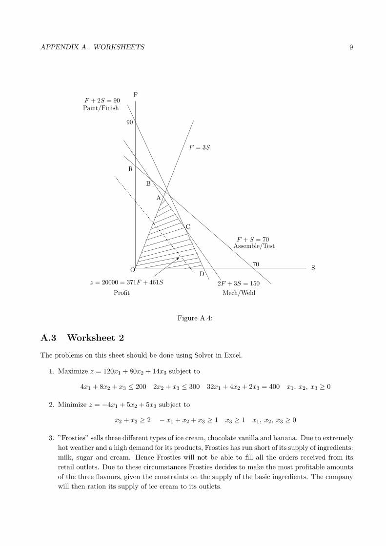
Carry out the Mathematics
(a) From Figure A.4 the dotted objective function is clearly a maximum at A or C. Bycalculating the coordinates of these points we find that z is maximum at A, which hascoordinates (16 2
3 , 50), giving z = 26233 13 . Thus the company should aim to produce 16
Body-Strong and 50 Body-Firm machines. This will yield £25926. (without roundinganalysis)
(b) If the constraint F ≤ 3S is dropped the feasible region is enlarged and becomes the polygonORBACD. z will now be maximum at B or R. Calculating the coordinates of thesepoints and calculating the corresponding values of z the maximum occurs at B which hascoordinates (10, 60) with z = £26870. Thus if the constraint is lifted the company canincrease its profit.
(c) Assuming all constraints are in place, as in (a), then the maximum at A can be increasedby causing A to move away from the origin. This can be done by increasing the effort inthe Machine and Welding department.
APPENDIX A. WORKSHEETS 9
A
C
D
R
B
F = 3S
F + S = 70
2F + 3S = 150
F + 2S = 90
Assemble/Test
Mech/Weld
Paint/Finish
......
......
......
......
......
......
......
......
......
......
......
.
z = 20000 = 371F + 461S
>
Profit
S
F
70
90
O
Figure A.4:
A.3 Worksheet 2
The problems on this sheet should be done using Solver in Excel.
1. Maximize z = 120x1 + 80x2 + 14x3 subject to
4x1 + 8x2 + x3 ≤ 200 2x2 + x3 ≤ 300 32x1 + 4x2 + 2x3 = 400 x1, x2, x3 ≥ 0
2. Minimize z = −4x1 + 5x2 + 5x3 subject to
x2 + x3 ≥ 2 − x1 + x2 + x3 ≥ 1 x3 ≥ 1 x1, x2, x3 ≥ 0
3. ”Frosties” sells three different types of ice cream, chocolate vanilla and banana. Due to extremelyhot weather and a high demand for its products, Frosties has run short of its supply of ingredients:milk, sugar and cream. Hence Frosties will not be able to fill all the orders received from itsretail outlets. Due to these circumstances Frosties decides to make the most profitable amountsof the three flavours, given the constraints on the supply of the basic ingredients. The companywill then ration its supply of ice cream to its outlets.
APPENDIX A. WORKSHEETS 10
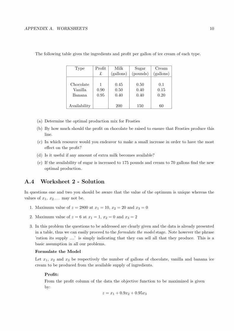
The following table gives the ingredients and profit per gallon of ice cream of each type.
Type Profit Milk Sugar Cream£ (gallons) (pounds) (gallons)
Chocolate 1 0.45 0.50 0.1Vanilla 0.90 0.50 0.40 0.15Banana 0.95 0.40 0.40 0.20
Availability 200 150 60
(a) Determine the optimal production mix for Frosties
(b) By how much should the profit on chocolate be raised to ensure that Frosties produce thisline.
(c) In which resource would you endeavor to make a small increase in order to have the mosteffect on the profit?
(d) Is it useful if any amount of extra milk becomes available?
(e) If the availability of sugar is increased to 175 pounds and cream to 70 gallons find the newoptimal production.
A.4 Worksheet 2 - Solution
In questions one and two you should be aware that the value of the optimum is unique whereas thevalues of x1, x2 . . . may not be.
1. Maximum value of z = 2800 at x1 = 10, x2 = 20 and x3 = 0
2. Maximum value of z = 6 at x1 = 1, x2 = 0 and x3 = 2
3. In this problem the questions to be addressed are clearly given and the data is already presentedin a table, thus we can easily proceed to the formulate the model stage. Note however the phrase’ration its supply ....’ is simply indicating that they can sell all that they produce. This is abasic assumption in all our problems.
Formulate the Model
Let x1, x2 and x3 be respectively the number of gallons of chocolate, vanilla and banana icecream to be produced from the available supply of ingredients.
Profit:
From the profit column of the data the objective function to be maximized is givenby:
z = x1 + 0.9x2 + 0.95x3

APPENDIX A. WORKSHEETS 11
and represents the profit measured in £.
Constraints
From the other three columns of the table the constraints on the availability of materialare given by:
Mlk: 0.45x1+0.5x2+0.4x3 ≤ 200 Sug: 0.5x1+0.4x2+0.4x3 ≤ 150 Crm: 0.1x1+0.15x2+0.2x3 ≤ 60
As usual the non-negative condition x1, x2, x3 ≥ 0 is assumed.
Carry out the Mathematics
In this problem we simply run solver to give the output in Table A.5 and Table A.6.
Report
(a) From the Answer Report of Table A.5 the Final Value of the Target Cell is 341.25. Henceoptimal return is £341.25
From the Final Value column of the Adjustable Cells section, the optimal amount ofchocolate(x1) is zero, of vanilla(x2) is 300 gallons and banana(x3) is 75 gallons.
(b) Since the amount of chocolate is zero we can, by increasing the profit on chocolate, make itworthwhile to produce some. The reduced cost is precisely the amount by which this amountshould be changed to give a solution that involves a non-zero production of chocolate. Fromthe Adjustable Cells section of the Sensitivity Report the reduced cost for x1 is -0.0375. Thatis to say the profit on chocolate should be reduced by a negative amount, which we takeas an increase of 4p. Thus Frosties would need to adjust their price of chocolate to make aprofit of 1.04p/gallon.
(c) From the Constraints section of the Sensitivity Report the largest shadow (dual) priceis for Sugar. Thus for every 1 lb increase in the availability of sugar the company canmake an extra £1.875. Thus in the first instance an increase in sugar supply is the mostadvantageous.
(d) In the Constraints section of the Sensitivity Report the allowable increase for Milk is infinite(1E+30), no change in the solution no matter how much more milk we have. This alsofollows from the Constraints section of the Answer Report as Milk is listed as not Binding.That is to say there is already slack in the system at this optimum and increasing thesupply is only going to produce more slack.
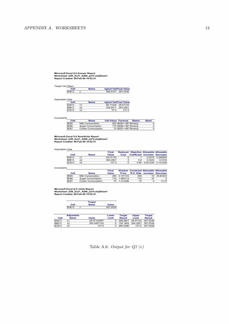
(e) In Table A.6 the new optimum value is now £397.05 and the production levels are 28.57gallons of Chocolate, 264.28 gallons of Vanilla and 137.5 gallons of Banana.

APPENDIX A. WORKSHEETS 12
Microsoft Excel 9.0 Answer Report
Worksheet: [OR_Ex21_ASW_p274.xls]Sheet1
Report Created: 08-Feb-06 09:52:23
Target Cell (Max)
Cell Name riginal ValuFinal Value
$H$13 z 2.85 341.25
Adjustable Cells
Cell Name riginal ValuFinal Value
$A$13 x1 1 0
$B$13 x2 1 300$C$13 x3 1 75
Constraints
Cell Name Cell Value Formula Status Slack
$E$5 Milk Consu 180 $E$5<=$F$Not Binding 20
$E$6 Sugar Cons 150 $E$6<=$F$Binding 0$E$7 Cream Con 60 $E$7<=$F$Binding 0
Microsoft Excel 9.0 Sensitivity Report
Worksheet: [OR_Ex21_ASW_p274.xls]Sheet1
Report Created: 08-Feb-06 09:52:23
Adjustable Cells
Final Reduced Objective Allowable Allowable
Cell Name Value Cost Coefficient Increase Decrease
$A$13 x1 0 -0.0375 1 0.0375 1E+30
$B$13 x2 300 0 0.9 0.05 0.0125$C$13 x3 75 0 0.95 0.021429 0.05
Constraints
Final Shadow Constraint Allowable Allowable
Cell Name Value Price R.H. Side Increase Decrease
$E$5 Milk Consu 180 0 200 1E+30 20
$E$6 Sugar Cons 150 1.875 150 10 30$E$7 Cream Con 60 1 60 15 3.75
Microsoft Excel 9.0 Limits Report
Worksheet: [OR_Ex21_ASW_p274.xls]Sheet1
Report Created: 08-Feb-06 09:52:23
Target
Cell Name Value
$H$13 z 341.25
Adjustable Lower Target Upper Target
Cell Name Value Limit Result Limit Result
$A$13 x1 0 0 341.25 2.96E-10 341.25
$B$13 x2 300 0 71.25 300 341.25$C$13 x3 75 0 270 75 341.25
Table A.5: Output for Q3. (a)-(d)
APPENDIX A. WORKSHEETS 13
Microsoft Excel 9.0 Answer Report
Worksheet: [OR_Ex21_ASW_p274.xls]Sheet1
Report Created: 08-Feb-06 10:02:21
Target Cell (Max)
Cell Name riginal ValuFinal Value
$H$13 z 384.9107 397.0536
Adjustable Cells
Cell Name riginal ValuFinal Value
$A$13 x1 85.71429 28.57143
$B$13 x2 292.8571 264.2857$C$13 x3 37.5 137.5
Constraints
Cell Name Cell Value Formula Status Slack
$E$5 Milk Consumption 200 $E$5<=$F$Binding 0
$E$6 Sugar Consumption 175 $E$6<=$F$Binding 0$E$7 Cream Consumption 70 $E$7<=$F$Binding 0
Microsoft Excel 9.0 Sensitivity Report
Worksheet: [OR_Ex21_ASW_p274.xls]Sheet1
Report Created: 08-Feb-06 10:02:21
Adjustable Cells
Final Reduced Objective Allowable Allowable
Cell Name Value Cost Coefficient Increase Decrease
$A$13 x1 28.57143 0 1 0.0375 0.290625
$B$13 x2 264.2857 0 0.9 0.2325 0.0125$C$13 x3 137.5 0 0.95 0.021429 0.121429
Constraints
Final Shadow Constraint Allowable Allowable
Cell Name Value Price R.H. Side Increase Decrease
$E$5 Milk Consumption 200 0.107143 200 10 30.83333
$E$6 Sugar Consumption 175 1.660714 175 37 5$E$7 Cream Consumption 70 1.214286 70 5 13.75
Microsoft Excel 9.0 Limits Report
Worksheet: [OR_Ex21_ASW_p274.xls]Sheet1
Report Created: 08-Feb-06 10:02:21
Target
Cell Name Value
$H$13 z 397.0536
Adjustable Lower Target Upper Target
Cell Name Value Limit Result Limit Result
$A$13 x1 28.57142857 0 368.4821 28.57143 397.0536
$B$13 x2 264.2857143 0 159.1964 264.2857 397.0536$C$13 x3 137.5 0 266.4286 137.5 397.0536
Table A.6: Output for Q3 (e)

APPENDIX A. WORKSHEETS 14
A.5 Worksheet 3
1. The standard or canonical form of the linear programming problem is:
Given Ax = b such that x ≥ 0, b ≥ 0 maximize or minimize z = cT x
Write the following problems in standard form:
(a) Maximize z = −x1 − 2x2 + x3 subject to:
3x2 + 2x1 + x3 ≤ 3 (i) x1 + x2 + x3 ≤ 1 (ii) x1, x2 x3 ≥ 0
(b) Maximize z = 2x1 + 4x2 + x3 subject to:
x1 + x2 + x3 = 1 2x1 + x2 − x3 ≤ 2 x1 + x2 ≥ −4 x2 + x3 ≥ 1
With x1, x2 ≥ 0 and x3 unrestricted
2. Use Solver to find the solutions to the problems in Q1.
(note that it is not necessary to write the problem in standard form to use solver - this is doneautomatically inside solver
3. Given:
x1
(12
)+ x2
(31
)+ x3
(11
)=
(43
)
use the direct method of solving simultaneous equations (non-matrix) to obtain the three basicsolutions to the problem.
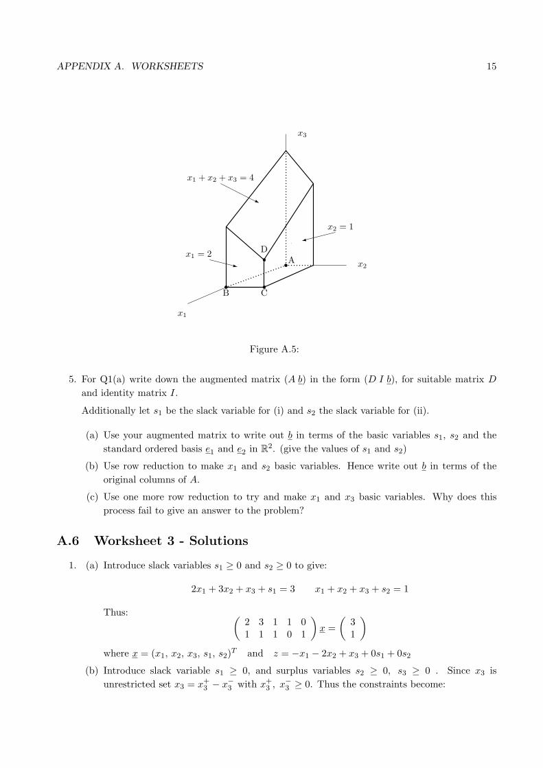
4. (This question was intended to give you a geometric idea of basic feasible solutions, however itseem to just cause more problems - I suggest you ignore it if its not obvious. Its not the sort ofquestion that will appear in the exam.)
The points satisfying
x1 + x2 + x3 ≤ 4 x1 ≤ 2 x2 ≤ 1 and x1, x2, x3 ≥ 0 (A.5)
are all the points inside and on the solid shown in Fig. A.5.
Writing Eqs(A.5) in the form x1 + x2 + x3 + s1 = 4, x1 + s2 = 2 and x2 + s3 = 1 write downthe basic variables at each of the points A, B, C and D in Fig. A.5.
Apply row reduction to
1 1 1 1 0 0 41 0 0 0 1 0 20 1 0 0 0 1 1
to emulate moving from A to B, B to C and C to D. Use your matrix to write down the values ofthe basic variables at each point. Do these values agree with what you expect from the diagram.
APPENDIX A. WORKSHEETS 15
...
...
...
...
...
...
...
...
...
...
...
...
...
...
.
.........................
...........x1 = 2
x1
x2
x3
x2 = 1
x1 + x2 + x3 = 4
j
9
z A
B C
D
Figure A.5:
5. For Q1(a) write down the augmented matrix (A b) in the form (D I b), for suitable matrix D
and identity matrix I.
Additionally let s1 be the slack variable for (i) and s2 the slack variable for (ii).
(a) Use your augmented matrix to write out b in terms of the basic variables s1, s2 and thestandard ordered basis e1 and e2 in R2. (give the values of s1 and s2)
(b) Use row reduction to make x1 and s2 basic variables. Hence write out b in terms of theoriginal columns of A.
(c) Use one more row reduction to try and make x1 and x3 basic variables. Why does thisprocess fail to give an answer to the problem?
A.6 Worksheet 3 - Solutions
1. (a) Introduce slack variables s1 ≥ 0 and s2 ≥ 0 to give:
2x1 + 3x2 + x3 + s1 = 3 x1 + x2 + x3 + s2 = 1
Thus: (2 3 1 1 01 1 1 0 1
)x =
(31
)
where x = (x1, x2, x3, s1, s2)T and z = −x1 − 2x2 + x3 + 0s1 + 0s2
(b) Introduce slack variable s1 ≥ 0, and surplus variables s2 ≥ 0, s3 ≥ 0 . Since x3 isunrestricted set x3 = x+
3 − x−3 with x+3 , x−3 ≥ 0. Thus the constraints become:

APPENDIX A. WORKSHEETS 16
x1 + x2 + x+3 − x−3 = 1
2x1 + x2 − x+3 + x−3 + s1 = 2
−x1 − x2 + s2 = 4x2 + x+
3 − x−3 − s3 = 1
⇒
1 1 1 −1 0 0 02 1 −1 1 1 0 0
−1 −1 0 0 0 1 00 1 1 −1 0 0 −1
x =
1241
where x = (x1, x2, x+3 , x−3 , s1, s2, s3)T and z = 2x1 + 4x2 + x+
3 − x−3 + 0s1 + 0s2 + 0s3
2. (a) Use solver to give x1 = x2 = 0, x3 = 1, zmax = 1
(b) Use solver to give x1 = 0, x2 = 1.5, x3 = −0.5, zmax = 2.5
3. The three basic solutions are obtained as follows
(a) Selecting the first two columns and setting x3 = 0 we need to solve:
x1
(12
)+ x2
(31
)=
(43
)⇒ x1 + 3x2 = 4
2x1 + x2 = 3⇒ x1 = x2 = 1
Basic solution: x1 = x2 = 1, x3 = 0
(b) Selecting the first and last column and setting x2 = 0 gives:
x1
(12
)+ x3
(11
)=
(43
)⇒ x1 + x3 = 4
2x1 + x3 = 3⇒ x1 = −1, x3 = 5
Basic solution: x1 = −1, x2 = 0, x3 = 5
(c) Selecting the last tow column and setting x1 = 0 gives:
x2
(31
)+ x3
(11
)=
(43
)⇒ 3x2 + x3 = 4
x2 + x3 = 3⇒ x2 = 1/2, x3 = 5/2
Basic solution: x1 = 0, x2 = 1/2, x3 = 5/2
4. The basic variables are A(s1, s2, s3), B(s1, x1, s3), C(s1, x1, x2) and D(x3, x1, x2).
At A:
1 1 1 [1] 0 0 41 0 0 0 [1] 0 20 1 0 0 0 [1] 1
⇒ s1 = 4, s2 = 2, s3 = 1
To move to B introduce x1 and take out s2. Thus row reduce to make column 1 (the x1 col)= e2. (notation: standard ordered basis ei.)
At B:
0 1 1 [1] −1 0 2[1] 0 0 0 1 0 20 1 0 0 0 [1] 1
⇒ x1 = 2, s1 = 2, s3 = 1
To move to C introduce x2 and take out s3. Thus row reduce to make column 2 (the x2 col)= e3.

APPENDIX A. WORKSHEETS 17
At C:
0 0 1 [1] −1 −1 1[1] 0 0 0 1 0 20 [1] 0 0 0 1 1
⇒ x1 = 2, x2 = 1, s1 = 1
To move to D introduce x3 and take out s1. Thus row reduce to make column 3 (the x3 col)= e1. (no row reduction actually necessary, just relabel pivot)
At D:
0 0 [1] 1 −1 −1 1[1] 0 0 0 1 0 20 [1] 0 0 0 1 1
⇒ x1 = 2, x2 = 1, x3 = 1
Recall that non-basic variable are, by design, always zero. Thus picking off the x-coordinates ofthe points A, B, C and D from above gives:
At A (x1, x2, x3) = (0, 0, 0) At B (x1, x2, x3) = (2, 0, 0)At C (x1, x2, x3) = (2, 1, 0) At D (x1, x2, x3) = (2, 1, 1)
These are seen to correspond to the coordinates of the points on the diagram.
5.
(D I b) =
2 3 1
... [1] 0... 3
1 1 1... 0 [1]
... 1
(a) In general:
b =(
31
)= x1
(21
)+ x2
(31
)+ x3
(11
)+ s1
(10
)+ s2
(01
)(A.6)
Starting with basic variables s1 and s2, thus all the x variables have been set to zero gives
b =(
31
)= s1 e1 + s2 e2 ⇒ s1 = 3, s2 = 1
(b) Introduce x1 and take out s2. That is to say use row reduction to make col(1) = e2.(
0 1 −1 [1] −2 1[1] 1 1 0 1 1
)
With x1 and s1 as basic variables and all the others zero, the pivots [1] in the matrix givex1 = 1 and s1 = 1. Thus from Eq(A.6)
(31
)= b = x1
(21
)+ s1
(10
)=
(21
)+
(10
)
(c) Introduce x3 and take out s1 by making col(3)=e1:(
0 −1 [1] −1 2 −1[1] 2 0 1 −1 2
)

APPENDIX A. WORKSHEETS 18
Thus the basic variables are x1 = 2 and x3 = −1, all other variables set equal to zero. ThusEq(A.6) gives:
(31
)= b = x1
(21
)+ x3
(11
)= 2
(21
)−
(11
)
This is not a feasible solution since the variable are not all non-negative, namely x3 < 0.
A.7 Worksheet 4
1. Simplex - all slack variables
Given
4x1 + 3x2 + 3x3 ≤ 12 3x1 + 4x2 + 4x3 ≤ 12 x3 ≤ 1 x1, x2, x3 ≥ 0
this question asks you to investigate the maximization of the objective function
z = 2x1 + 2x2 + 3x3
using the Simplex Method as follows:
(a) Write the constraints in the standard form Ax = b where A is a suitable matrix of the form(D I) and I is the identity matrix. x and b are suitable column vectors such that x ≥ 0and b ≥ 0.
(b) Set up the Simplex Tableau and hence solve the problem.
(c) Use the final tableau to
i. Obtain the dual (shadow) values corresponding to each of the first three constraint.
ii. Find the feasible ranges of each of the components of b
iii. The range of optimality for each of the coefficients in the objective function z.
2. Simplex - Artificial variables
Consider the problem:
Maximize z = 2x1 + x2 subject to
x1 + x2 ≤ 2 (i) x1 + 3x2 ≥ 3 (ii) x1, x2 ≥ 0
(a) Introducing a slack variable s1 and a surplus variable s2 write the problem in the formAx = b, and z = cT x, where x, b ≥ 0.
Why is it not possible to initially use s1 and s2 as basic variables?
(b) Introduce an additional artificial variable a1 ≥ 0, such that a1 and s1 can be used as initialbasic variables.
(c) Introducing the variable M in the objective function write down the Simplex Tableau forthis problem. Hence solve using the Simplex Method.

APPENDIX A. WORKSHEETS 19
(d) Using the optimal tableau write down the shadow values for the problem.
(e) Solve the problem graphically.
Indicate the order in which the Simplex Method visited the corners of the feasible region.
Use your graph to find the maximum value of z if in constraint (i) the righthand side isincreased to 3. Is this consistent with your results for the dual values in (d).
A.8 Worksheet 4 - Solutions
1. (a) Introducing slack variables s1, s2, s3 ≥ 0 the inequalities become:
4x1 + 3x2 + 3x3 + s1 = 12, 3x1 + 4x2 + 4x3 + s2 = 12, x3 + s3 = 1, x1, x2, x3 ≥ 0
In the required matrix form:
Ax = (D|I)x =
4 3 3 1 0 03 4 4 0 1 00 0 1 0 0 1
x =
12121
= b
Where x = (x1, x2, x3, s1, s2, s3)T and z = cT x = 2x1 + 2x2 + 3x3 + 0s1 + 0s2 + 0s3.
(b) The first simplex tableau:
x1 x2 x3 s1 s2 s3 b ba
Basic Var cj 2 2 3 0 0 0 ratio
s1 0 4 3 3 1 0 0 12 4s2 0 3 4 4 0 1 0 12 3s3 0 0 0 1 0 0 1 1 [1]zj 0 0 0 0 0 0 z =∆z 2 2 [3] 0 0 0 0
Table A.7: Since this is a maximization problem, add to the basic set the variable corresponding to themaximum positive value in the final row. Remove from the basic set the variable corresponding to thesmallest non-negative value in the final column.
In the final row (variable columns), [3] is the maximum value, thus introduce x3 into thebasic set. The ratio column consists of the d column elements divided by the correspondingterms in the x3 column. Select the variable corresponding to the smallest non-negativevalue in the ratio column, namely s3, to remove from the basic set.
Row reduce to make the x3 column into the old s3 column, that is to say row reduce tomake the x3 column equal to e3.
In Table A.8 there are two positive maximum values in the final row, hence it is equallyacceptable to add either x1 or x2 to the basic set: I have add x1 to the basic set. Thesmallest non-negative value in the final column corresponds to s1, hence remove s1 fromthe basic set.
APPENDIX A. WORKSHEETS 20
x1 x2 x3 s1 s2 s3 d da
Basic Var cj 2 2 3 0 0 0 ratio
s1 0 4 3 0 1 0 −3 9 [9/4]s2 0 3 4 0 0 1 −4 8 8/3x3 3 0 0 1 0 0 1 1 ∞zj 0 0 3 0 0 3 z =∆z [2] 2 0 0 0 −3 3
Table A.8: This table shows the next step is to add x1 to the basic set and remove s1.
x1 x2 x3 s1 s2 s3 d da
Basic Var cj 2 2 3 0 0 0 ratio
x1 2 1 3/4 0 1/4 0 −3/4 9/4 3s2 0 0 7/4 0 −3/4 1 −7/4 5/4 [5/7]x3 3 0 0 1 0 0 1 1 ∞zj 2 3/2 3 1/2 0 3/2 z =∆z 0 [1/2] 0 −1/2 0 −3/2 15/2
Table A.9: This table shows that the next step is to add x2 to the basic set and remove s2.
Thus row reduce to make the x1 column equal to the old s1 column, that is to say makecolumn 1 equal to e1.Thus row reduce to make the x2 column equal to the old s2 column, that is to say column2 becomes e2
x1 x2 x3 s1 s2 s3 d da
Basic Var cj 2 2 3 0 0 0 ratio
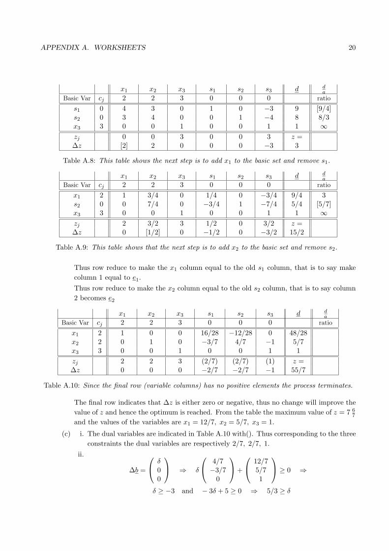
x1 2 1 0 0 16/28 −12/28 0 48/28x2 2 0 1 0 −3/7 4/7 −1 5/7x3 3 0 0 1 0 0 1 1zj 2 2 3 (2/7) (2/7) (1) z =∆z 0 0 0 −2/7 −2/7 −1 55/7
Table A.10: Since the final row (variable columns) has no positive elements the process terminates.
The final row indicates that ∆z is either zero or negative, thus no change will improve thevalue of z and hence the optimum is reached. From the table the maximum value of z = 7 6
7
and the values of the variables are x1 = 12/7, x2 = 5/7, x3 = 1.
(c) i. The dual variables are indicated in Table A.10 with(). Thus corresponding to the threeconstraints the dual variables are respectively 2/7, 2/7, 1.
ii.
∆b =
δ00
⇒ δ
4/7−3/7
0
+
12/75/71
≥ 0 ⇒
δ ≥ −3 and − 3δ + 5 ≥ 0 ⇒ 5/3 ≥ δ

APPENDIX A. WORKSHEETS 21
Thus−3 ≤ δ ≤ 5/3 ⇒ 12− 3 ≤ b1 ≤ 12 + 5/3 ⇒ 9 ≤ b1 ≤ 13
23
∆b =
0δ0
⇒ δ
−3/74/70
+
12/75/71
≥ 0 ⇒
−3δ + 12 ≥ 0 ⇒ δ ≤ 4 and 4δ + 5 ≥ 0 ⇒ δ ≥ −5/4
Thus
−5/4 ≤ δ ≤ 4 ⇒ 12− 5/4 ≤ b2 ≤ 12 + 4 ⇒ 1034≤ b2 ≤ 16
∆b =
00δ
⇒ δ
0−11
+
12/75/71
≥ 0 ⇒
−δ + 5/7 ≥ 0 ⇒ δ ≤ 5/7 and δ + 1 ≥ 0 ⇒ δ ≥ −1
Thus−1 ≤ δ ≤ 5/7 ⇒ 1− 1 ≤ b3 ≤ 1 + 5/7 ⇒ 0 ≤ b3 ≤ 1
57
iii. To calculate the range of optimality for each of the coefficients in the original objectivefunction replace in turn the c values in the final tableau with α. To ensure the tableauremains optimal impose the condition on α such that the final row remains non-positive.For the c-coefficient of x1 in the objective function z the optimal table (Table A.10)becomes:
x1 x2 x3 s1 s2 s3 d da
Basic Var cj α 2 3 0 0 0 ratio
x1 α 1 0 0 16/28 −12/28 0 48/28x2 2 0 1 0 −3/7 4/7 −1 5/7x3 3 0 0 1 0 0 1 1zj α 2 3 4α/7− 6/7 −3α/7 + 8/7 1 z =∆z 0 0 0 −4α/7 + 6/7 3α/7− 8/7 −1 31+12α
7
Table A.11: The final row must remain non-positive for the table to remain optimal
From Table A.11 −4α/7 + 6/7 ≤ 0 and 3α/7 − 8/7 ≤ 0 must be satisfied forthe table to remain optimal. Thus 3/2 ≤ α ≤ 8/3
The interval of optimality for c1, the c-coefficient of x1, is [32 , 83 ].
Repeating the above with, in turn, α replacing the c-coefficient of x2 and then x3 gives:
Range of optimality for c2 is [32 , 83 ] and for c3 is [2, ∞).

APPENDIX A. WORKSHEETS 22
2. (a) Introducing s1, s2 ≥ 0 the inequalities become:
x1 + x2 + s1 = 2 (i) x1 + 3x2 − s2 = 3 (ii) x1, x2 ≥ 0
which can be written in matrix form:(
1 1 1 01 3 0 −1
)x =
(23
)x ≥ 0
where x = (x1, x2, s1, s2)T and the objective function z = 2x1 + x2 + 0s1 + 0s2.
The simplex method tries to starts with s1 and s2 as basic variables by setting x1 = x2 = 0.However (ii) implies that s2 = −3 < 0, thus this is not a valid starting point as it is not inthe feasible region.
(b) The problem of finding a feasible starting value is overcome by the introduction of anartificial variable a1 ≥ 0 into (ii). (ii) becomes:
x1 + 3x2 − s2 + a1 = 3.
Thus initially the non-basic variable are taken to be x1, x2, s2 (all set equal to zero) andthe basic variables are s1 and a1, which clearly have the values 2 and 3 respectively. Thekey point is that the starting values are now in the feasible set.
(c) As a1 is an artificial variable we require it to vanish from the final solution, this can bedone by introducing M >> 0 into the objective function (relabel z′)as:
z′ = x1 + 3x2 + 0s1 + 0s2 −Ma1
Clearly the −Ma1 term will tend to suppress the value of z, thus when maximizing, thisterm will have the least affect when a1 = 0. That is to say the maximization process willtend to force a1 to zero.
To set up the first tableau order the variables so that the ’body’ of the table lookslike (D|I). That is to say the first three variables are the non-basic variables and the lasttwo are the basic variables.
x1 x2 s2 s1 a1 d da
Basic Var cj 2 1 0 0 −M ratio
s1 0 1 1 0 1 0 2 2a1 −M 1 3 −1 0 1 3 [1]zj −M −3M M 0 −M z′ =∆z 2 + M [1 + 3M ] −M 0 0 −3M
Table A.12: For sufficiently large M maximum positive value in the last row is [1 + 3M ], thus add x2
to the basic set. Smallest non-negative term in the final column corresponds to a1, hence remove a1
from the basic set.
To bring in x2 and take out a1 row reduce to make the x2 column equal to the old a1
column, namely e2. (See Table A.13)
APPENDIX A. WORKSHEETS 23
x1 x2 s2 s1 a1 d da
Basic Var cj 2 1 0 0 −M ratio
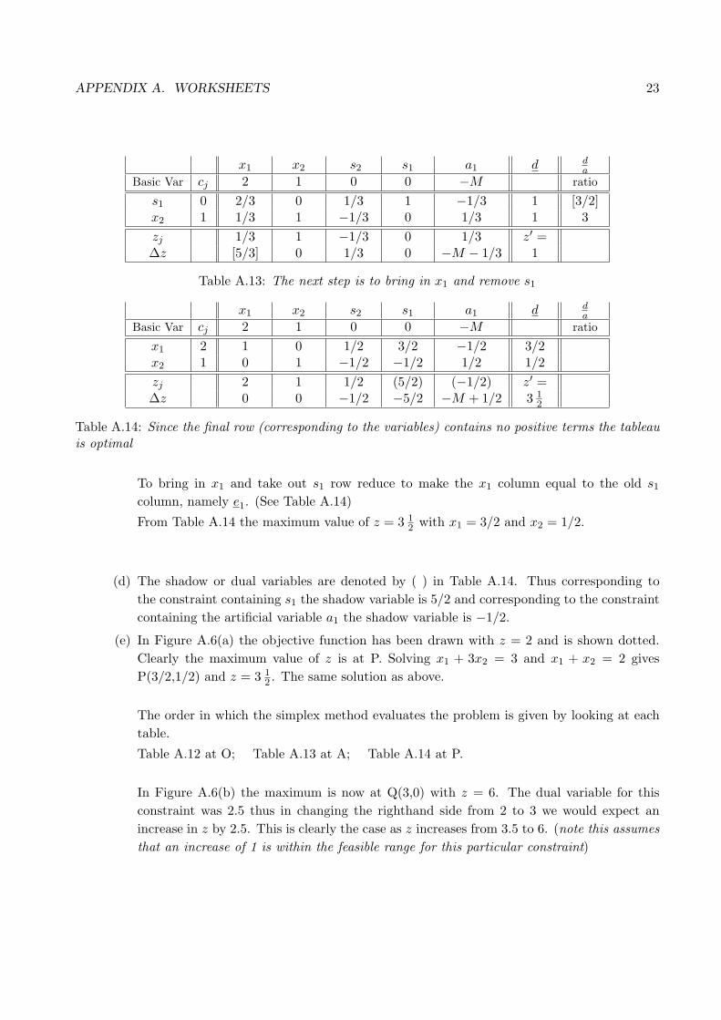
s1 0 2/3 0 1/3 1 −1/3 1 [3/2]x2 1 1/3 1 −1/3 0 1/3 1 3zj 1/3 1 −1/3 0 1/3 z′ =∆z [5/3] 0 1/3 0 −M − 1/3 1
Table A.13: The next step is to bring in x1 and remove s1
x1 x2 s2 s1 a1 d da
Basic Var cj 2 1 0 0 −M ratio
x1 2 1 0 1/2 3/2 −1/2 3/2x2 1 0 1 −1/2 −1/2 1/2 1/2zj 2 1 1/2 (5/2) (−1/2) z′ =∆z 0 0 −1/2 −5/2 −M + 1/2 3 1
2
Table A.14: Since the final row (corresponding to the variables) contains no positive terms the tableauis optimal
To bring in x1 and take out s1 row reduce to make the x1 column equal to the old s1
column, namely e1. (See Table A.14)
From Table A.14 the maximum value of z = 3 12 with x1 = 3/2 and x2 = 1/2.
(d) The shadow or dual variables are denoted by ( ) in Table A.14. Thus corresponding tothe constraint containing s1 the shadow variable is 5/2 and corresponding to the constraintcontaining the artificial variable a1 the shadow variable is −1/2.
(e) In Figure A.6(a) the objective function has been drawn with z = 2 and is shown dotted.Clearly the maximum value of z is at P. Solving x1 + 3x2 = 3 and x1 + x2 = 2 givesP(3/2,1/2) and z = 3 1
2 . The same solution as above.
The order in which the simplex method evaluates the problem is given by looking at eachtable.
Table A.12 at O; Table A.13 at A; Table A.14 at P.
In Figure A.6(b) the maximum is now at Q(3,0) with z = 6. The dual variable for thisconstraint was 2.5 thus in changing the righthand side from 2 to 3 we would expect anincrease in z by 2.5. This is clearly the case as z increases from 3.5 to 6. (note this assumesthat an increase of 1 is within the feasible range for this particular constraint)

APPENDIX A. WORKSHEETS 24
......................................................
x1
x2
P
O
A
B
2 3
z = 2 = 2x1 + x2x1 + x2 = 2
x1 + 3x2 = 3
1
2
C
......................................................
x1
x2
z = 4 = 2x1 + x2x1 + x2 = 3
x1 + 3x2 = 3
Q
3
O
A
2 3
1
C
(a) (b)
Figure A.6: Feasible region shown hashed
APPENDIX A. WORKSHEETS 25
A.9 Worksheet 5
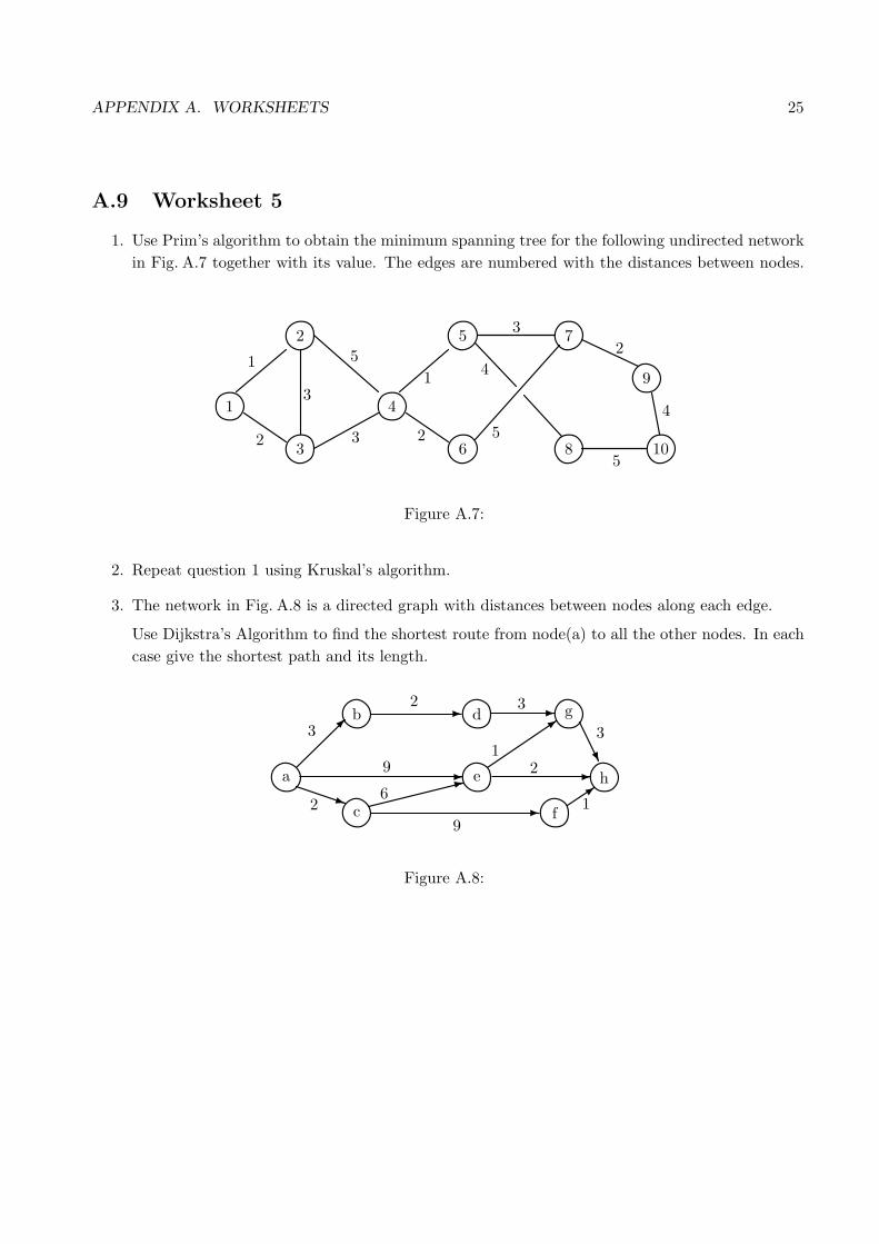
1. Use Prim’s algorithm to obtain the minimum spanning tree for the following undirected networkin Fig. A.7 together with its value. The edges are numbered with the distances between nodes.
1
2
3
4
5
6
7
8
9
10
1
2
3
5
3
1
2
3
5
4
5
2
4
Figure A.7:
2. Repeat question 1 using Kruskal’s algorithm.
3. The network in Fig. A.8 is a directed graph with distances between nodes along each edge.
Use Dijkstra’s Algorithm to find the shortest route from node(a) to all the other nodes. In eachcase give the shortest path and its length.
a
b
c
d
e
g
h
f
µ- -
- -U
3-
:
3
q
3
2 3
31
2
19
6
9
2
Figure A.8:

APPENDIX A. WORKSHEETS 26
4. The network in Fig. A.9 is a mixed graph with edges numbered with the distance between thenodes. Use Floyd’s algorithm to find the shortest routes between all pairs of the nodes givingthe routes and distances.
1
2
3
4
>
w-
2
3
1
4
3
6
Figure A.9:
5. Use the min cut max flow theorem to construct by inspection a possible maximum flow inthe following mixed network Fig. A.10(a); numbers refer to capacities. Give the value of themaximum flow.
S
a
c
d
b
d
f
T
µ
-
R+-
s-R
>
-
}
3
3
6
2
4
7
2
3
1
9 6
2 5
Fig (a)
S
a
b
c
d eT
1
-
z
?
*
-
6:q ?
:q
3
1 6
33
2
5
7
24
4 3
Fig (b)
Figure A.10:
6. Use the Ford-Fulkerson algorithm to find a maximum flow from source S to sink T for thedirected network in Fig. A.10(b); numbers refer to capacities.

APPENDIX A. WORKSHEETS 27
A.10 Worksheet 5 - Solutions
1. Figure A.11 shows the minimal spanning tree formed using Prim’s algorithm. The length of thetree is 22.
1
2
1
2
3
1
2
3
4
1
2
3
4
5
1
2
3
4
5
6
1 1 1
11 11
2 2
2 2 2
3
3 3
1
2
3
4
5
6
1 1
2 23
73
1
2
3
4
5
6
1 1
2 23
73
84
1
2
3
4
5
6
1 1
2 23
73
84 9
2
1
2
3
4
5
6
1 1
2 23
73
84 9
2
10
4
Figure A.11: Prim’s Algorithm adding the closest node at each stage
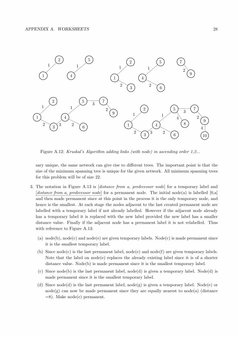
2. Figure A.12 shows the construction of the minimal spanning tree for the same network as Q1but using Kruskal’s algorithm.
This process has given the same spanning tree, however minimum spanning trees are not neces-
APPENDIX A. WORKSHEETS 28
1
2
4
51 1
1
2
4
51 1
3 6
7
9
2 2
2
1
2
4
51 1
3 6
7
9
2 2
2
3
3
1
2
4
51 1
3 6
7
9
2 2
2
3
3
8
10
4
4
Figure A.12: Kruskal’s Algorithm adding links (with node) in ascending order 1,2...
sary unique, the same network can give rise to different trees. The important point is that thesize of the minimum spanning tree is unique for the given network. All minimum spanning treesfor this problem will be of size 22.
3. The notation in Figure A.13 is [distance from a, predecessor node] for a temporary label and[distance from a, predecessor node] for a permanent node. The initial node(a) is labelled [0,a]and then made permanent since at this point in the process it is the only temporary node, andhence is the smallest. At each stage the nodes adjacent to the last created permanent node arelabelled with a temporary label if not already labelled. However if the adjacent node alreadyhas a temporary label it is replaced with the new label provided the new label has a smallerdistance value. Finally if the adjacent node has a permanent label it is not relabelled. Thuswith reference to Figure A.13:
(a) node(b), node(c) and node(e) are given temporary labels. Node(c) is made permanent sinceit is the smallest temporary label.
(b) Since node(c) is the last permanent label, node(e) and node(f) are given temporary labels.Note that the label on node(e) replaces the already existing label since it is of a shorterdistance value. Node(b) is made permanent since it is the smallest temporary label.
(c) Since node(b) is the last permanent label, node(d) is given a temporary label. Node(d) ismade permanent since it is the smallest temporary label.
(d) Since node(d) is the last permanent label, node(g) is given a temporary label. Node(e) ornode(g) can now be made permanent since they are equally nearest to node(a) (distance=8). Make node(e) permanent.

APPENDIX A. WORKSHEETS 29
a
b
c
d
e
g
h
f
µ- -
- -U
3-
:
3
q
3
2 3
31
2
1
9
6
9
2
a
b
c
d
e
g
h
f
µ- -
- -U
3-
:
3
q
3
2 3
31
2
1
9
6
9
2[0,a] [0,a]
[3,a]
[9,a]
[2,a]
[3,a]
[2,a]
[9,a]
[8,c]
[11,c]
(a) (b)
a
b
c
d
e
g
h
f
µ- -
- -U
3-
:
3
q
3
2 3
31
2
1
9
6
9
2
[3,a]
[2,a]
[9,a]
[8,c]
[11,c]
(c)
[0,a]
[5,b]
a
a
b
c
d
e
g
h
f
µ- -
- -U
3-
:
3
q
3
2 3
31
2
1
9
6
9
2
[3,a]
[2,a]
[9,a]
[8,c]
[11,c]
(d)
[0,a]
[5,b] [8,d]
b
c
d
e
g
h
f
µ- -
- -U
3-
:
3
q
3
2 3
31
2
1
9
6
9
2
[3,a]
[2,a]
[9,a]
[8,c]
[11,c]
(e)
[0,a]
[5,b] [8,d]
[10,e]
a
b
c
d
e
g
h
f
µ- -
- -U
3-
:
3
q
3
2 3
31
2
1
9
6
9
2
[3,a]
[2,a]
[9,a]
[8,c]
[11,c]
(f)
[0,a]
[5,b] [8,d]
[10,e]
Figure A.13:
(e) Since node(e) is the last permanent label, node(h) is given a temporary label. Node(g) ismade permanent since it is the smallest temporary label.
(f) Since node(g) is the last permanent label we look to give node(h) a label. Since thetemporary label on node(h) is less than the incoming label no relabelling takes place.Node(h) is made permanent since it is the smallest temporary label.
Finally since node(h) is the last permanent label we look to give node(f) a label. Since theincoming label is the same value as the temporary label already on node(f) no change is made.Node(f) is then made permanent.
The process terminates since all nodes are now permanent.
The labels can be used to trace back the path from each node to node(a) to give:
a → b : 3, a → b → d : 5, a → b → d → g : 8, a → c → e : 8,

APPENDIX A. WORKSHEETS 30
a → c : 2, a → c → f : 11, a → c → e → h : 10.
4. Floyd’s method requires two matrices, one representing the state of the current network (Di)and one monitoring the changes made (Mi).
Start at node(1):
If di,1 + d1,j < di,j , that is to say if there a shorter path via node(1), then make a replacementpath.
D0 =
∗ 2 3 6∞ ∗ 3 13 3 ∗ 4∞ ∞ 4 ∗
M0 =
1 2 3 41 2 3 41 2 3 41 2 3 4
For node(1) no replacement necessary.
Move to node(2).
If di,2 + d2,j < di,j , that is to say if there is a shorter path via node(2), then make a replacementpath.
D1 =
∗ 2 3 −6−3
∞ ∗ 3 13 3 ∗ 4∞ ∞ 4 ∗
M1 =
1 2 3 −4−2
1 2 3 41 2 3 41 2 3 4
Move to node(3):
If di,3 + d3,j < di,j , that is to say if there is a shorter path via node(3), then make a replacementpath.
D2 =
∗ 2 3 3−∞−6 ∗ 3 1
3 3 ∗ 4−∞−7 −∞−7 4 ∗
M2 =
1 2 3 2−1−3 2 3 41 2 3 4−1−3 −2−3 3 4
Move to node(4):
If di,4 + d4,j < di,j , that is to say if there is a shorter path via node(4), then make a replacementpath.
D3 =
∗ 2 3 36 ∗ 3 13 3 ∗ 47 7 4 ∗
M3 =
1 2 3 23 2 3 41 2 3 43 3 3 4
For node(4) no replacement necessary.
Thus D3 gives the matrix of shortest distances between nodes and M3 gives us the route for thispath from node to node.
APPENDIX A. WORKSHEETS 31
1 → 2 = 2, 2 → 3 → 1 = 6, 1 → 3 = 3, 3 → 1 = 3, 1 → 2 → 4 = 3, 4 → 3 → 1 = 7
2 → 3 = 3, 3 → 2 = 3, 2 → 4 = 1, 4 → 3 → 2 = 7, 3 → 4 = 4, 4 → 3 = 4
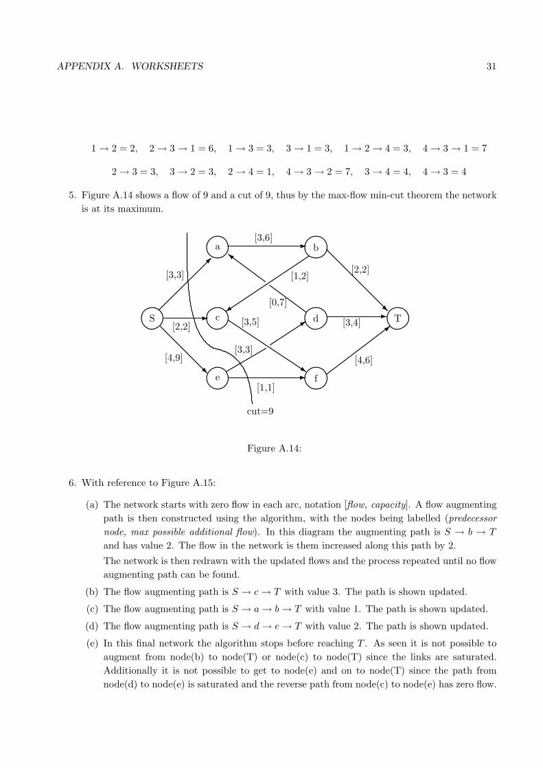
5. Figure A.14 shows a flow of 9 and a cut of 9, thus by the max-flow min-cut theorem the networkis at its maximum.
S
a
c
e
b
d
f
T
µ
-
R+-
s-R
>
-
}
3
[3,3]
[3,6]
[2,2]
[3,4]
[0,7]
[1,2]
[3,3]
[1,1]
[4,9] [4,6]
[2,2] [3,5]
cut=9
Figure A.14:
6. With reference to Figure A.15:
(a) The network starts with zero flow in each arc, notation [flow, capacity]. A flow augmentingpath is then constructed using the algorithm, with the nodes being labelled (predecessornode, max possible additional flow). In this diagram the augmenting path is S → b → T
and has value 2. The flow in the network is them increased along this path by 2.
The network is then redrawn with the updated flows and the process repeated until no flowaugmenting path can be found.
(b) The flow augmenting path is S → c → T with value 3. The path is shown updated.
(c) The flow augmenting path is S → a → b → T with value 1. The path is shown updated.
(d) The flow augmenting path is S → d → e → T with value 2. The path is shown updated.
(e) In this final network the algorithm stops before reaching T . As seen it is not possible toaugment from node(b) to node(T) or node(c) to node(T) since the links are saturated.Additionally it is not possible to get to node(e) and on to node(T) since the path fromnode(d) to node(e) is saturated and the reverse path from node(c) to node(e) has zero flow.

APPENDIX A. WORKSHEETS 32
S
a
b
c
d e
T
1
-z
?
*
-
6:q ?
:q
[0,3]
[0,1] [0,6]
[0,3][0,3]
[0,2]
[0,5]
[0,7]
[0,2][0,4]
[0,4][0,3]
(S,∞)
(S,1)
(S,2)
(b,2)
(S,5)
(S,3)
[2,2]
[2,3]
(a)
S
a
b
c
d e
T
1
-z
?
*
-
6:q ?
:q
[0,3]
[0,1] [0,6]
[2,3][0,3]
[2,2]
[0,5]
[0,7]
[0,2][0,4]
[0,4][0,3]
(S,∞)
(S,1)
(a,1)
(c,3)
(S,5)
(S,3)
[3,3]
[3,5]
(b)
[0,1] [0,6]
S
a
b
c
d e
T
1
-z
?
*
-
6:q ?
:q
[0,3]
(d,2)
(c,2)
[3,3][0,3]
[2,2]
[0,7]
[0,2][0,4]
[0,4]
[3,5]
[3,3]
(a,1)
(b,1)
(S,2)
(S,3)
S
[1,6] a
(c)
[1,1]
b
(S,∞)
c
d e
T
1
-z
?
*
-
6:q ?
:q
[0,3]
(d,2)
[3,3]
[0,3]
[2,2]
[0,7]
[0,2][0,4]
[0,4]
[3,5]
[3,3][2,3]
(e,2)
(S,2)
(S,3)
[1,6]
(d)
[1,1](S,∞)
[2,2][2,4]
S
a
b
c
d e
T
1
-z
?
*
-
6:q ?
:q
[2,2]
(c,2)
[2,4]
[3,3]
[0,3]
[2,2]
[2,3]
[0,7][0,4]
[3,5]
[3,3]
(e,2)
(S,2)
(S,1)
[1,6]
(e)
[1,1](S,∞)
cut = 8
(S,1)
[2,3]
Figure A.15:
Hence the final network with maximum flow of 8 is seen in Figure A.15(d).
Just for interest I have included a cut in Figure A.15(e) with value 8. This is therefore a minimumcut since we know the max flow is also 8. Note that the flow from node(e) to node(c) does notcontribute to the value of the cut as it is in the reverse direction, that is to say it is leaving andnot entering the cut region containing T .

APPENDIX A. WORKSHEETS 33
A.11 Worksheet 6 - Class Example - No solution given
1. Using the methodology of dynamic programming we are required to find for the network below:
(i) The shortest path from node(1) to node(10).
(ii) The longest path from node(1) to node(10).
(iii) The path from node(1) to node (10) containing the shortest legs.
Before carrying out the calculations identify the following;
• Suitable stages for the process.
• The decision set Di at each stage.
• The state variables xi at each stage.
• The optimization function for each of (i), (ii) and (iii) above.
Carry out the calculations for (i), (ii) and (iii) by annotating Figures A.16 to A.18.
1
2
3
4 7
10
96
5 8
7
- -
R
w- -
µ
~
^
s- -
s
3
73
9
8
7
9
6
4
6
12
10
4
8
7
10
5
812
9
Figure A.16: Use for (i)

APPENDIX A. WORKSHEETS 34
1
2
3
4 7
10
96
5 8
7
- -
R
w- -
µ
~
^
s- -
s
3
73
9
8
7
9
6
4
6
12
10
4
8
7
10
5
812
9
Figure A.17: Use for (ii)
1
2
3
4 7
10
96
5 8
7
- -
R
w- -
µ
~
^
s- -
s
3
73
9
8
7
9
6
4
6
12
10
4
8
7
10
5
812
9
Figure A.18: Use for (iii)

Appendix B
Past Exam - May 2008
B.1 Question Paper
Full marks for correct solutions to any FOUR or the SIX questions - 214 hours
Question 1
The 2-bit computer company makes two types of computer, laptop and desktop. The computersare produced at 2-bit’s plant which is semi-automated and uses two manufacturing lines. Oneline assembles the computers whilst the other finishes, tests and packages them. The assemblytime for a laptop is 30 mins and 15 mins for a desktop. The finishing, packaging and testingtimes are 20 mins for a laptop and 20 mins for a desktop. Both assembly lines are available for8 hrs a day and it is projected that the profit on a laptop is £250 and on a desktop £100.
(i) Using the above data formulate and solve graphically the linear programming problem toobtain the maximum profit and the associated production levels in each 8 hour shift. Whymight this result not be acceptable to 2-bit?
[7 marks ]
(ii) Calculate the ’reduced costs’ associated with each type of computer. By how much wouldthe profit on a desktop need to be increased in order to make its production worthwhile.What would be the new maximum profit and production levels if this increase were made?
[3 marks ]
(iii) Write down the dual of the original problem, interpreting the dual decision variables, objec-tive function and constraints in terms of the production problem. Solve the dual problemgraphically and say if it is more profitable to make a marginal increase in the amount oftime on the assembly line or on the finishing, testing and packaging line.
[5 marks ]
(iv) The marketing people at 2-bit decide that it is desirable to produce at least as manydesktops as laptops.
35
APPENDIX B. PAST EXAM - MAY 2008 36
Express this constraint mathematically and hence amend your graph in (i) to show the newfeasible region.
What is the new maximum profit and the associated production levels in the 8 hour shift.
Comment on the total time used on each production line in the 8 hr shift and say why thismight be of concern to 2-bit.
[5 marks ]
(v) The management wish to ensure that in any 8 hr shift the difference in the times the twoproduction lines are in use is no more than 20 minutes. Express this constraint mathemat-ically and hence add to your graph to obtain the new levels of production and maximumprofit.
[5 marks ]
[25 marks in total ]
Question 2
The Finance Director of a large company has to make provision for the early retirement packagesthat are being offered to its employees over the next eight years. At the closing date for theacceptance of such packages the required funds (in £1000) at the start of each year are given inTable F.16.
year 1 2 3 4 5 6 7 8 9required funds 450 400 250 220 200 180 220 250 300
Table B.1: The amounts, in thousands of pound, required at the start of each year.
It is the Finance Director’s task to work out how much to set aside at the start of the process,including the amount required for the first payment, in order to meet the rest of the payments.In order to generate income the Finance Director can either invest in government bonds, whichmake payments at the end of each year, or invest in a cash account at 4.5% per annum. Thereare four types of bonds available to him, each with a par value of £100 but with different annualrates and different lengths of time to maturity. The details of the types of bonds are given inTable F.17.
Bond Price Annual Years toType £ Rate % Maturity
1 115 8.5 42 100 5.5 63 125 10.0 74 135 11.5 8
Table B.2: Present purchase price of the four types of bond, their various maturity dates and theirannual return.
APPENDIX B. PAST EXAM - MAY 2008 37
Let S be the total amount, in units of one thousand pounds, that has to be set aside, includingthe first payment, to fund the scheme.
Let b1, b2, b3 and b4 be the number of bonds of each type purchased at the start of the process;this is the only time at which bonds are purchased.
Let si i = 1, . . . 9 be the amount, in units of one thousand pounds, held as a cash deposit atthe start of each year. Note that money, generated as income from the investments or maturingbonds may be added to the cash account at the start of each year, or if necessary withdrawnfrom the cash account to help meet the payments. The variable s9 would represent money leftover at the end of the scheme.
Using the above variables construct, with explanation, the linear programming problem thatminimizes the total amount S that the Finance Director has to put aside.
[10 marks ]
The output from solving the linear programming problem is given in Table B.3. Since the bondsare of low value you may, for the purpose of this problem, ignore the fact that it is not possibleto buy parts of a bond. Answer the following question with reference to the output.
(i) How much did the Finance Director spend on bonds and how much cash did he initiallyplace on deposit. [3 marks ]
(ii) Determine the reduction of the amount of cash on deposit at the start of each subsequentyear. [3 marks ]
(iii) What is the initial value of £1 paid out at the start of year 9. [2 marks ]
(iv) If the amount required at the start of year 9 was in fact £400,000, by how much should S
be increased in order to accommodate this change. [2 marks ]
(v) What is the minimum decrease in the price of type 1 bonds to make their purchase worth-while?
[2 marks ]
(vi) As he is about to purchase the bonds the Finance director discovers that the price of type 4bonds has increased. What is the maximum increase that he can sustain in order to retainthe levels of his original investment strategy. [3 marks ]

APPENDIX B. PAST EXAM - MAY 2008 38
Variables
Name Final Reduced Objective Allowable Allowable
Value Cost Coefficient Increase Decrease
b1 0.00 0.00065 0.115 1E+30 0.00065
b2 1577.41 0.00000 0.1 0.00516 0.00162
b3 2264.17 0.00000 0.125 0.00177 0.00295
b4 2690.58 0.00000 0.135 0.00317 0.06852
s1 843.33 0.00000 1 0.00568 0.04905
s2 543.54 0.00000 0 0.00586 0.04941
s3 380.26 0.00000 0 0.00605 0.04979
s4 239.63 0.00000 0 0.00626 0.05020
s5 112.67 0.00000 0 7.22569 0.05063
s6 0.00 0.05109 0 1E+30 0.05109
s7 0.00 0.01686 0 1E+30 0.01686
s8 0.00 0.02973 0 1E+30 0.02973
s9 0.00 0.61453 0 1E+30 0.61453
Constraints
Name Final Shadow Constraint Allowable Allowable
Value Price R.H. Side Increase Decrease
Yr 2 400 0.95694 400 1E+30 881.28011
Yr 3 250 0.91573 250 1E+30 567.99849
Yr 4 220 0.87630 220 1E+30 397.36920
Yr 5 200 0.83856 200 1E+30 250.41159
Yr 6 180 0.80245 180 1E+30 117.74088
Yr 7 220 0.71901 220 2258.48423 166.41663
Yr 8 280 0.67191 280 1366.38296 249.05830
Yr 9 300 0.61453 300 1324.79739 300.00000
Objective function
Total Sum Value
S 2097.32062
Table B.3: Output from solving the Linear Programming problem.
[25 marks in total ]

APPENDIX B. PAST EXAM - MAY 2008 39
Question 3
(a) For a Euclidean space E define what is meant by:
(i) L is a line segment from x1 to x2.
(ii) C is a convex subset of E.
(iii) a is an extreme point of C
If A is an m× n matrix, m ≤ n, with m independent rows, define what is meant by sayingthat x is a basic feasible solution of Ax = b , x ≥ 0.
Given
1 0 0 10 1 0 10 0 1 1
x1
x2
x3
x4
=
321
x ≥ 0
obtain all basic feasible solutions.
State briefly how an extreme point and a basic feasible solution are related when solving alinear programming problem.
[8 marks ]
(b) Consider the following problem:
Maximize z = 2x1 + 3x2 + x3 subject to the constraints:
x1 + x2 + x3 ≤ 2 (1) x1 + 2x2 + 2x3 ≤ 3 (2) x1, x2 , x3 ≥ 0 (3)
(i) Introduce two slack variables s1 and s2 to write the problem in the matrix form:
Maximize z = cT x, subject to Ax = b, x ≥ 0.
State clearly the values of c, x, b and A. [2 marks ]
(ii) Write down the first Simplex Tableau. [4 marks ]
(iii) Find the optimal solution to the problem using the Simplex Method. [6 marks ]
(iv) From your final tableau find the feasible range for the righthand side of constraint (1).[5 marks ]
[25 marks in total ]

APPENDIX B. PAST EXAM - MAY 2008 40
Question 4
(a) A car hire company wishes to develop a strategy for replacing its fleet over a five yearperiod. The projected data for replacing a car is given in Table B.4. For example the costof replacing a car bought at the start of 2009 and replaced after two years at the start of2011 would be £6000. Assume that the scheme starts with a new car at the start of 2008and that the company only changes its cars at the end of one, two or three years. Thecompany’s objective is to find the minimum replacement cost and associated strategy sothat at the start of 2013 a new car is purchased.
Car bought Replacement cost (£) for given years of servicestart of 1 2 32008 4500 5500 85002009 4625 6000 90002010 4750 6500 95002011 4875 7000 −2012 5000 − −
Table B.4: Replacement cost of a car after a given number of years of service as a function of the year of itspurchase
Construct a network for this problem such that the solution to the problem is obtained byidentifying a path of minimum length through the network. Define carefully the meaningof the vertices and edges in your network. Hence demonstrate and use Dijkstra’s algorithmto solve the problem.
[12 marks ]
(b) For a graph G define the terms:
Tree, Spanning Tree, Minimal Spanning Tree.
[3 marks ]
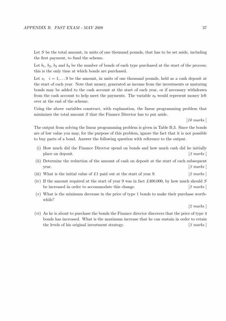
A University campus has two computing centres which must be connected by a direct link.The other buildings on the campus can either be connected directly to one or other of thecomputer centres or indirectly via the computing facilities of other buildings. The networkin Figure B.1 indicates the cost, in thousands of pounds, of making connections betweenthe various buildings. The computing centres are labeled C1, C2 and the other buildingsB1, . . . B8. As can be seen it is not possible to connect all building directly to each other orto a computing centre. Use Prim’s algorithm to establish the most cost effective methodof making the connections such that all the sites are in some way interconnected. Statethe level of this cost. Comment on the uniqueness of Prim’s algorithm in establishing theoptimum solution.
[10 marks ]
APPENDIX B. PAST EXAM - MAY 2008 41
C1
C2
B1
B2
B3
B4
B5
B6
B7
B8
65
1
4
2
6
2
3
63 3
4
72
14
5
2
3
Figure B.1: Diagram of potential connections.
[25 marks in total ]
Question 5
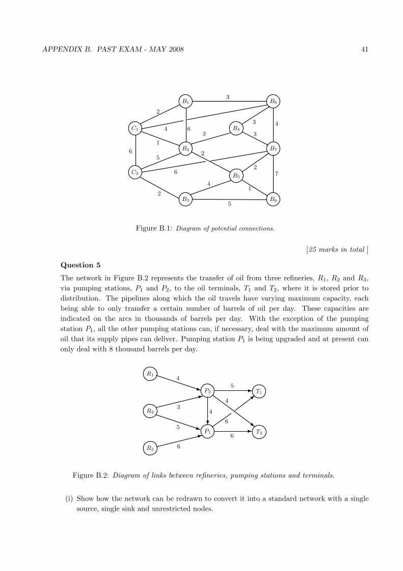
The network in Figure B.2 represents the transfer of oil from three refineries, R1, R2 and R3,via pumping stations, P1 and P2, to the oil terminals, T1 and T2, where it is stored prior todistribution. The pipelines along which the oil travels have varying maximum capacity, eachbeing able to only transfer a certain number of barrels of oil per day. These capacities areindicated on the arcs in thousands of barrels per day. With the exception of the pumpingstation P1, all the other pumping stations can, if necessary, deal with the maximum amount ofoil that its supply pipes can deliver. Pumping station P1 is being upgraded and at present canonly deal with 8 thousand barrels per day.
R1
R2
R3
T2
P2
P1
T1-
-~
q
:
>:
q?
5
6
4
4
3
5
6
6
4
Figure B.2: Diagram of links between refineries, pumping stations and terminals.
(i) Show how the network can be redrawn to convert it into a standard network with a singlesource, single sink and unrestricted nodes.
APPENDIX B. PAST EXAM - MAY 2008 42
Denoting the flow from node i to node j by fi,j , where i and j are the node labels, writedown an expression for the value of the flow in the network. [5 marks ]
(ii) Define what it meant by a ’Flow Augmenting Path’ for the standard networkdescribed in (i). [2 marks ]
(iii) Construct an example of a non-zero flow in your standard network. [2 marks ]
(iv) Use the Ford-Fulkerson algorithm to find the maximum flow in the network and show clearlyhow it is attained.
Hence state how much oil the refineries should produce and what storage capacity is neededat the terminals to ensure that the pipelines are best utilized.
[10 marks ]
(v) State the Max-Flow Min-Cut theorem and hence ’by inspection’ construct a cut that es-tablishes that the flow obtained in (iv) is indeed maximum.
[6 marks ]
[25 marks in total ]
Question 6
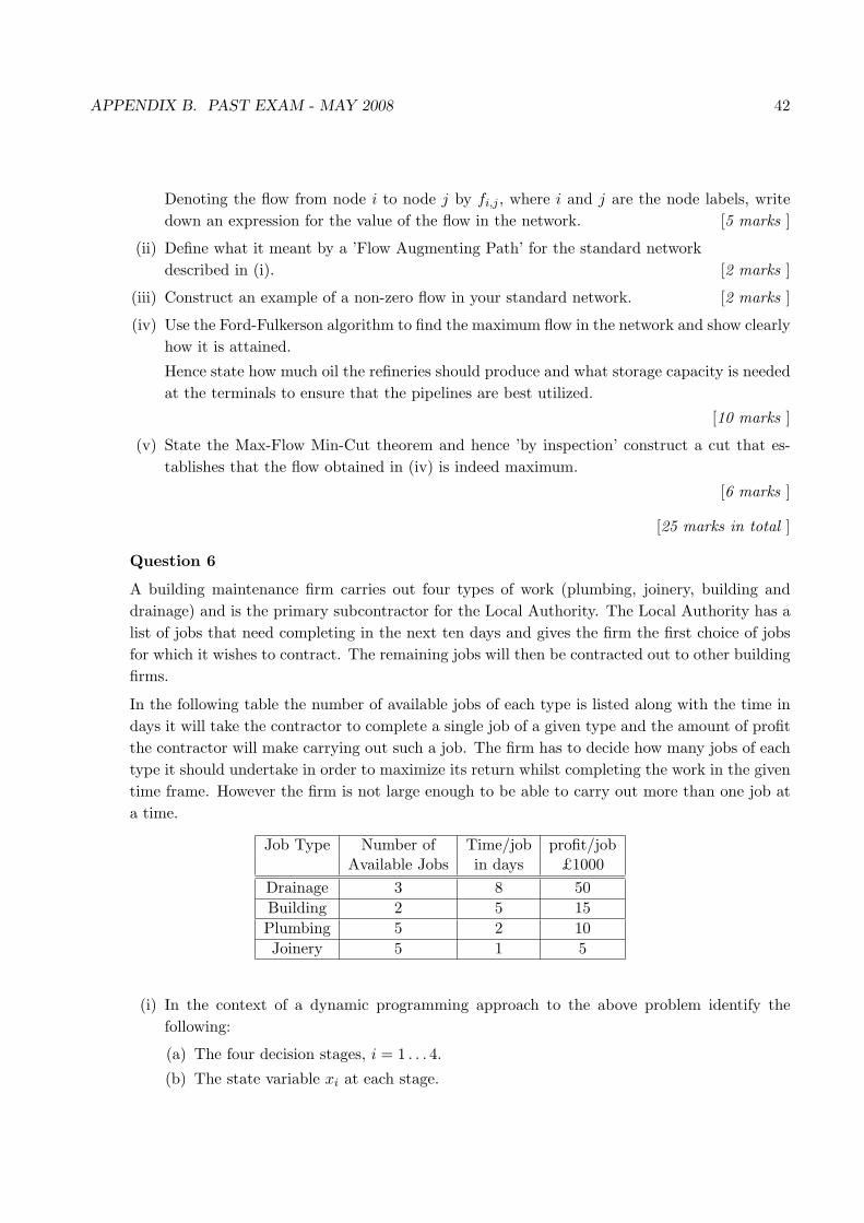
A building maintenance firm carries out four types of work (plumbing, joinery, building anddrainage) and is the primary subcontractor for the Local Authority. The Local Authority has alist of jobs that need completing in the next ten days and gives the firm the first choice of jobsfor which it wishes to contract. The remaining jobs will then be contracted out to other buildingfirms.
In the following table the number of available jobs of each type is listed along with the time indays it will take the contractor to complete a single job of a given type and the amount of profitthe contractor will make carrying out such a job. The firm has to decide how many jobs of eachtype it should undertake in order to maximize its return whilst completing the work in the giventime frame. However the firm is not large enough to be able to carry out more than one job ata time.
Job Type Number of Time/job profit/jobAvailable Jobs in days £1000
Drainage 3 8 50Building 2 5 15Plumbing 5 2 10Joinery 5 1 5
(i) In the context of a dynamic programming approach to the above problem identify thefollowing:
(a) The four decision stages, i = 1 . . . 4.
(b) The state variable xi at each stage.

APPENDIX B. PAST EXAM - MAY 2008 43
(c) The decisions at each stage.
(d) An optimization functional fi(xi) and a defining backward recursion relation.
[7 marks ]
(ii) Draw a suitable network to illustrate the above problem, indicating clearly the four stages.Hence use your network, by making suitable annotations at each node, to obtain the optimalstrategy and return for the problem. (Show all your working.)
[18 marks ]
[25 marks in total ]

APPENDIX B. PAST EXAM - MAY 2008 44
B.2 Solutions
Solutions May 2007
1. (i) Let xL and xD be the number of laptops and desktops produced each day; thus xL, xD ≥ 0
The profit is given by: z = 250xL + 100xD
Minutes assembling = 30xL + 15xD ≤ 480 ⇒ 2xL + xD ≤ 32
Minutes finishing = 20xL + 20xD ≤ 480 ⇒ xL + xD ≤ 24
xL + xD = 242xL + xD = 32
Q(0, 24)P (8, 16)
R(16, 0)
xL
xD
Calculating z at P , Q and R gives:zQ = 2400, zP = 3600, zR = 4000Thus the maximum profit is £4000 con-sisting of 16 laptops and 0 desktops. Pro-ducing no desktops may not be acceptableto 2-bit.
[7 marks ]
(ii) Reduced cost for laptops is zero since xL 6= 0 at optimum.
Since xD = 0 at optimum, change coefficient of xD in z such that the objective functionhas the same slope as 2xL + xD = 32, thus making P optimum. Let α be the reduced cost,thus:
− 250100− α
= −2 ⇒ α = −25
Thus the profit on a desktop must be increased by £25 to make its production worthwhile.The production is 8 laptops and 16 desktops with a profit of £4000.
[3 marks ]
(iii) The dual problem: Let yA be the cost/min on the assembly line and yF be the cost perminute on the finishing line. Then the dual problem is:
Minimize z = 480yA + 480yF subject to:
30yA + 20yF ≥ 250 15yA + 20yF ≥ 100 yA, yF ≥ 0
30yA + 20yF is the cost of producing 1 laptop and 15yA + 20yF is the cost of producing 1desktop, in each case this cost is greater than the profit. [3 marks ]

APPENDIX B. PAST EXAM - MAY 2008 45
yA
yF
3yA + 2yF = 253yA + 4yF = 20
P (0, 25/2)
Q(25/3, 0)
The value of z at P and Q is given byzP = 6000 and zQ = 4000. The minimumz is £4000, with yA = 25/3 and yF = 0.Thus better to increase the time on theassembly line.
[2 marks ]
(iv)
xL + xD = 242xL + xD = 32
Q(0, 24)P (8, 16)
R(16, 0)
xL
xD
xD = xL
S
The constraint is xD ≥ xL hence addxD = xL to the graph in (i). AtS(102
3 , 1023) the value of z = 37331
3 , thusmax at S.The time on the assembly line is now 480mins and on the finishing line 4262
3mins.
The finishing line staff are idle for toolong.
[5 marks ]
(v) The constraint is given by:
|30xL + 15xD − 20xL − 20xD| ≤ 20
⇒ −20 ≤ 10xL − 5xD ≤ 20
Plot the two equations on the graph in(iv). New max at T (9, 14) with z = 3650Hence 2-bit should produce 9 laptops and14 desktops per day.
xL + xD = 242xL + xD = 32
Q(0, 24)P
R(16, 0)
xL
xD
xD = xL
T
10xL − 5xD = 20
S
10xL − 5xD = −20
[5 marks ]
2. We wish to minimize the outlay, S, at the start of the first year, given by:
S = 450 + 0.115b1 + 0.100b2 + 0.125b3 + 0.135b4 + s1 [2 marks ]
We must have sufficient funds to meet the payments at the start of each subsequent year. (Sinceany excess funds can be placed on deposit the constraints can be just = though ≤ also acceptablein the following.)
• start yr 2: 400 = 0.0085b1 + 0.0055b2 + 0.01b3 + 0.0115b4 + 1.045s1 − s2
• start yr 3: 250 = 0.0085b1 + 0.0055b2 + 0.01b3 + 0.0115b4 + 1.045s2 − s3

APPENDIX B. PAST EXAM - MAY 2008 46
• start yr 3: 220 = 0.0085b1 + 0.0055b2 + 0.01b3 + 0.0115b4 + 1.045s3 − s4
• type 1 bonds now mature thus at start of year 4:200 = 0.1085b1 + 0.0055b2 + 0.01b3 + 0.0115b4 + 1.045s4 − s5
• start yr 5: 180 = 0.0055b2 + 0.01b3 + 0.0115b4 + 1.045s5 − s6
• type 2 bonds now mature thus at start of year 6:220 = 0.1055b2 + 0.01b3 + 0.0115b4 + 1.045s6 − s7
• type 3 bonds now mature thus at start of year 7:250 = 0.11b3 + 0.0115b4 + 1.045s7 − s8
• type 4 bonds now mature thus at start of year 8:300 = 0.1115b4 + 1.045s8 − s9
All variables are greater or equal to zero. [8 marks ]
(i) s1 = £843, 330 place initially on deposit. Spend on bonds=£803,990.55 [3 marks ]
(ii) Reductions: start of year 2 £299,790; start of year 3 £163,280; start of year 4 £140,630;start of year 5 £126,960; start of year 6 £112,670; and then no more cash deposits.
[3 marks ]
(iii) This is the dual price for year 9 payment = £0.61453 ≈ 61.5p. [2 marks ]
(iv) This is the present day value of £100,000 at year 9 = 100000× 0.61453 = £61, 453[2 marks ]
(v) Reduced cost = 0.00065, thus we need the price of type 1 bond to decrease by 65p.[2 marks ]
(vi) Allowed increase of type 4 bond is 0.00317, thus we can sustain an increase of £3.17 andstill retain our buying levels etc. [3 marks ]
3. (a) (i) L = {x ∈ E : x = x1 + λ(x2 − x1) 0 ≤ λ ≤ 1}(ii) C is a convex subset of E if for any two points x1 and x2 in C the line segment joining
the two points lies entirely in C.(iii) a is an extreme point of C if a ∈ C and there is no line segment in C such that a is an
interior point of the line segment.[3 marks ]
A basic feasible solution is a solution of Ax = b, x ≥ 0 formed by selecting m independentcolumns of A, setting the variables associated with the other n−m columns equal to zero,and solving the m independent equations so formed. [1 mark ]
Directly: x4 = 0, x1 = 3, x2 = 2, x3 = 1 feasible.
1 0 0 1 30 1 0 1 20 0 1 1 1
→
1 0 0 1 3−1 1 0 0 −1−1 0 1 0 −2
x1 = 0, x2 = −1, x3 = −2, x4 = 3 not fsbl
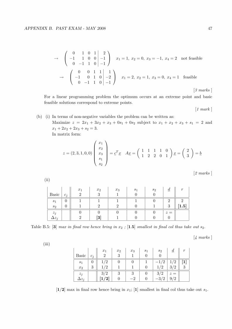
APPENDIX B. PAST EXAM - MAY 2008 47
→
0 1 0 1 2−1 1 0 0 −1
0 −1 1 0 −1
x1 = 1, x2 = 0, x3 = −1, x4 = 2 not feasible
→
0 0 1 1 1−1 0 1 0 −2
0 −1 1 0 −1
x1 = 2, x2 = 1, x3 = 0, x4 = 1 feasible
[3 marks ]
For a linear programming problem the optimum occurs at an extreme point and basicfeasible solutions correspond to extreme points.
[1 mark ]
(b) (i) In terms of non-negative variables the problem can be written as:Maximize z = 2x1 + 3x2 + x3 + 0s1 + 0s2 subject to x1 + x2 + x3 + s1 = 2 andx1 + 2x2 + 2x3 + s2 = 3.In matrix form:
z = (2, 3, 1, 0, 0)
x1
x2
x3
s1
s2
= cT x Ax =(
1 1 1 1 01 2 2 0 1
)x =
(23
)= b
[2 marks ]
(ii)
x1 x2 x3 s1 s2 d rBasic cj 2 3 1 0 0
s1 0 1 1 1 1 0 2 2s2 0 1 2 2 0 1 3 [1.5]zj 0 0 0 0 0 z =
∆zj 2 [3] 1 0 0 0
Table B.5: [3] max in final row hence bring in x2 ; [1.5] smallest in final col thus take out s2.
[4 marks ]
(iii)x1 x2 x3 s1 s2 d r
Basic cj 2 3 1 0 0s1 0 1/2 0 0 1 −1/2 1/2 [1]x2 3 1/2 1 1 0 1/2 3/2 3zj 3/2 3 3 0 3/2 z =
∆zj [1/2] 0 −2 0 −3/2 9/2
[1/2] max in final row hence bring in x1; [1] smallest in final col thus take out s1.
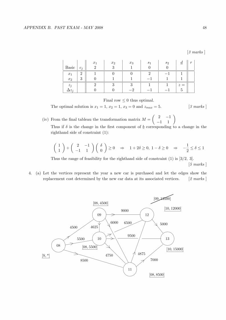
APPENDIX B. PAST EXAM - MAY 2008 48
[3 marks ]
x1 x2 x3 s1 s2 d rBasic cj 2 3 1 0 0x1 2 1 0 0 2 −1 1x2 3 0 1 1 −1 1 1zj 2 3 3 1 1 z =
∆zj 0 0 −2 −1 −1 5
Final row ≤ 0 thus optimal.The optimal solution is x1 = 1, x2 = 1, x3 = 0 and zmax = 5. [3 marks ]
(iv) From the final tableau the transformation matrix M =(
2 −1−1 1
)
Thus if δ is the change in the first component of b corresponding to a change in therighthand side of constraint (1):
(11
)+
(2 −1−1 1
)(δ0
)≥ 0 ⇒ 1 + 2δ ≥ 0, 1− δ ≥ 0 ⇒ −1
2≤ δ ≤ 1
Thus the range of feasibility for the righthand side of constraint (1) is [3/2, 3].[5 marks ]
4. (a) Let the vertices represent the year a new car is purchased and let the edges show thereplacement cost determined by the new car data at its associated vertices. [2 marks ]
08
09
10
11
13
12
4500
8500
5500
9000
5000
7000
4875
6000
4750
9500
65004625
[S, *]
[08, 4500][09, 13500]
[10, 12000]
[10, 15000]
[08, 8500]
[08, 5500]

APPENDIX B. PAST EXAM - MAY 2008 49
[4 marks ]
Dijkstra’s Method
Notation: Temporary label: [previous vertex, dist back to (08)]; underline to make intoa permanent label.
Start at (08) with permanent label [S, *]
Label all vertices adjacent to (08) with temporary labels. Make smallest, [08, 4500] on (09),permanent
Label all vertices adjacent to (09) that don’t have a permanent label, with a temporarylabel, replacing any existing temporary labels of higher value. Make smallest temporarylabel, [08, 5500] on (10), permanent.
Label all vertices adjacent to (10) that don’t have a permanent label, with a temporarylabel, replacing any existing temporary labels of higher value. Make smallest temporarylabel, [08, 8500] on (11), permanent.
Label all vertices adjacent to (11) that don’t have a permanent label, with a temporarylabel, replacing any existing temporary labels of higher value. Make smallest temporarylabel, [10, 12000] on (12), permanent.
Finally make (13) permanent. [5 marks ]
The permanent label [10, 15,000] on (13) corresponds to a minimum cost of £15,000, andas indicated by the network, the shortest route 08 → 10 → 13 corresponds to a strategy ofreplacing after 2 years and then again after 3 years. [1 marks ]
(b) A tree is a simply connected subgraph of G with no cycles. [1 mark ]
A spanning tree for a connected graph G is a subgraph of G that is a tree containing allnodes of G. [1 mark ]
A minimum spanning tree for G is a spanning tree for G such that the sum of the valuesof its edges is a minimum. [1 mark ]
First connect the two centres together, since this direct link is mandatory. From the pointof view of Prim’s algorithm this coupled pair is considered as a single node. [2 marks ]

APPENDIX B. PAST EXAM - MAY 2008 50
C1
C2
6
C1
C2
6 B21
C1
C2
6 B21
B22C1
C2
6 B21
B22
B32
C1
C2
6 B21
B22
B32
B52
C1
C2
6 B21
B22
B32
B52
B8
1
C1
C2
6 B21
B22
B32
B52
B8
1
B7 B4
B8
2
3
3
[ 5 marks ]
The minimum cost is £22,000 [2 marks ](if they do not connect C1 and C2 initially they get £20,000 - allow follow through)Prim’s does not give a unique tree since at each stage the vertex added may not be unique,however the value of the final spanning tree is unique. If the values of each edge is differentthen the minimal spanning tree is unique. [1 mark ]
5.
S
R1
R2
R3
P2
P ′1 P ′′1
T1
T2
T
4
4
4
4
11
8
68
6
6
65
5
3
10
.......................................................................
cut = 15
Figure B.3:
(i) Introduce a source S with outgoing edges to R1, R2 and R3 with capacities equal to thetotal output capacity of respectively each of the vertices R1, R2 and R3...see figure
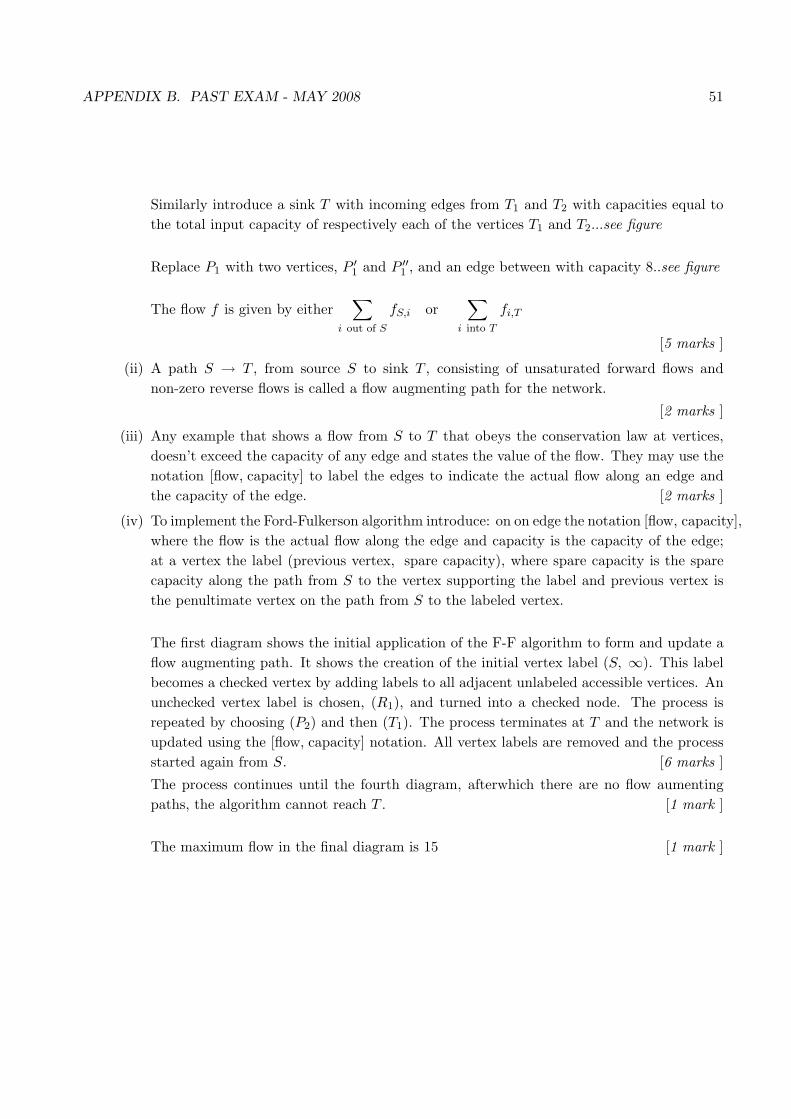
APPENDIX B. PAST EXAM - MAY 2008 51
Similarly introduce a sink T with incoming edges from T1 and T2 with capacities equal tothe total input capacity of respectively each of the vertices T1 and T2...see figure
Replace P1 with two vertices, P ′1 and P ′′
1 , and an edge between with capacity 8..see figure
The flow f is given by either∑
i out of S
fS,i or∑
i into T
fi,T
[5 marks ]
(ii) A path S → T , from source S to sink T , consisting of unsaturated forward flows andnon-zero reverse flows is called a flow augmenting path for the network.
[2 marks ]
(iii) Any example that shows a flow from S to T that obeys the conservation law at vertices,doesn’t exceed the capacity of any edge and states the value of the flow. They may use thenotation [flow, capacity] to label the edges to indicate the actual flow along an edge andthe capacity of the edge. [2 marks ]
(iv) To implement the Ford-Fulkerson algorithm introduce: on on edge the notation [flow, capacity],where the flow is the actual flow along the edge and capacity is the capacity of the edge;at a vertex the label (previous vertex, spare capacity), where spare capacity is the sparecapacity along the path from S to the vertex supporting the label and previous vertex isthe penultimate vertex on the path from S to the labeled vertex.
The first diagram shows the initial application of the F-F algorithm to form and update aflow augmenting path. It shows the creation of the initial vertex label (S, ∞). This labelbecomes a checked vertex by adding labels to all adjacent unlabeled accessible vertices. Anunchecked vertex label is chosen, (R1), and turned into a checked node. The process isrepeated by choosing (P2) and then (T1). The process terminates at T and the network isupdated using the [flow, capacity] notation. All vertex labels are removed and the processstarted again from S. [6 marks ]
The process continues until the fourth diagram, afterwhich there are no flow aumentingpaths, the algorithm cannot reach T . [1 mark ]
The maximum flow in the final diagram is 15 [1 mark ]

APPENDIX B. PAST EXAM - MAY 2008 52
S
R1
R2
R3
P2
P ′1 P ′′1
T1
T2
T
4
4
4
4
11
8
68
6
6
65
5
3
10
(S,∞)
(S, 4)
(R1, 4) (P2, 4)
(T1, 4)
[4,4] [4,4]
[4,5]
[4,11]
S
R1
R2
R3
P2
P ′1 P ′′1
T1
T2
T
(S, 8)4
4
(S, 6)
(R3, 6)
8
68
6
6
65
(P ′1, 6)
3
10
(S,∞)
(P ′′1 , 6)
(P ′′1 , 6)
(T2, 6)
[4,4] [4,4]
[4,5]
[4,11]
[6,6]
[6,6]
[6,8] [6,6] [6,10]
(S, 8)
(S, 6)
(P2, 4) (P2, 4)
S
R1
R2
R3
P2
P ′1 P ′′1
T1
T2
T
(S, 8)4
4
(R2, 3)
(R2, 5)
8
65
[9,10]
3 [3,4]
(S,∞)
(P2, 3)
[3,3]
(P2, 1)
(T2, 3)
[4,4] [4,4]
[4,5]
[4,11]
[3,8]
S
R1
R2
[6,6]
[6,6]
[6,8] [6,6] [6,10]
R3
P2
P ′1 P ′′1
T1
T2
T
(S, 2)[3,3]
4
(P ′1, 2)(R2, 2)
[3,4]
[3,8][6,11]
[9,10]65
[2,6]
[8,8](S,∞)[2,5]
(P ′′1 , 2)
(T1, 2)
[4,4] [4,4]
[4,5]
[4,11]
[5,8]
[6,6]
[6,6]
[6,8] [6,6]
The refineries R1, R2 and R3 should produce respectively 4000, 5000 and 6000 barrels perday. The terminals T1 and T2 will respectively need to be able to store or deal with 6000and 9000 barrels per day. [2 marks ]
(v) The maximum flow= minimum cut [1 mark ]
The cut in Figure B.3 has the value 15 which is the same as the flow found by the F-Fmethod. Thus 15 is indeed the max flow. Note that in the cut the flow from P2 → P ′
1 isnot in the direction from S to T and thus is not included in the value of the cut.[5 marks ]

APPENDIX B. PAST EXAM - MAY 2008 53
6. (i) (a) Let the first stage, i = 1, be the decision of how many drainage type jobs to undertake.Let the second stage, i = 2, be the decision of how many building type jobs to under-take.Let the third stage, i = 3, be the decision of how many plumbing type jobs to undertake.Let the fourth stage, i = 4, be the decision of how many joinery type jobs to undertake.
[2 marks ]
(b) Let xi be the number of remaining days available when selecting type i jobs.[1 mark ]
(c) Let di be the number of type i jobs allocated at stage i. [1 mark ]
(d) Let fi(xi) = the maximum return from stage i to the end of stage 4, for given inputxi. Thus
fi(xi) = max{fi+1(xi+1) + di × profit on job type i } f5(x5) = 0
where xi+1 = xi − di × time for job i [3 marks ]
(ii) Label each vertex as (xi), indicating the number of available days at the start of each stage.At the end of stage 4 the vertices show the number of days not used.
Label each edge with di, the number of jobs of type i allocated.
Use the vertex labeling [fi(xi), xi+1] [3 marks ]
10
2
10
2
0
5
10
2
0
1
3
5
4
6
8
10
0
1
3
5
stage 1 stage 2 stage 3 stage 4
1
0
0
2
1
0
0
1
0
2
1
0
3
2
1
0
2
0
1
3
5
4
5
5
5
[10,0]
[0,0]
[5,0]
[15,0]
[25,0]
[20,0]
[25,1]
[25,3]
[25,5]
[50,2]
[25,1]
[0,0]
[10,2]
[10,2]
[50,10]
[60,2]
.............
...........
...........
...........
-

APPENDIX B. PAST EXAM - MAY 2008 54
[8 marks ]
Show working to demonstrate how the maximum is selected at each vertex. For example
f3(2) = max{f4(2) + 0× 10 = 10; f4(0) + 1× 10 = 10} = 10
Note the choice of the label [10,2] on vertex (2) at stage 3 is not unique, it could have been[10,0], giving the same profit but a different strategy. [5 marks ]
The maximum path in the figure is given by
10 2 2 2 0- - - -1 0 0 2
representing that the company undertake 1 drainage job and 2 joinery jobs at a profit of£60,000.(other strategies giving the same profit are possible) [2 marks ]
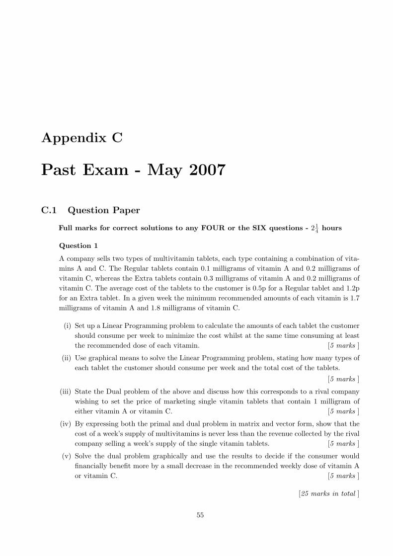
Appendix C
Past Exam - May 2007
C.1 Question Paper
Full marks for correct solutions to any FOUR or the SIX questions - 214 hours
Question 1
A company sells two types of multivitamin tablets, each type containing a combination of vita-mins A and C. The Regular tablets contain 0.1 milligrams of vitamin A and 0.2 milligrams ofvitamin C, whereas the Extra tablets contain 0.3 milligrams of vitamin A and 0.2 milligrams ofvitamin C. The average cost of the tablets to the customer is 0.5p for a Regular tablet and 1.2pfor an Extra tablet. In a given week the minimum recommended amounts of each vitamin is 1.7milligrams of vitamin A and 1.8 milligrams of vitamin C.
(i) Set up a Linear Programming problem to calculate the amounts of each tablet the customershould consume per week to minimize the cost whilst at the same time consuming at leastthe recommended dose of each vitamin. [5 marks ]
(ii) Use graphical means to solve the Linear Programming problem, stating how many types ofeach tablet the customer should consume per week and the total cost of the tablets.
[5 marks ]
(iii) State the Dual problem of the above and discuss how this corresponds to a rival companywishing to set the price of marketing single vitamin tablets that contain 1 milligram ofeither vitamin A or vitamin C. [5 marks ]
(iv) By expressing both the primal and dual problem in matrix and vector form, show that thecost of a week’s supply of multivitamins is never less than the revenue collected by the rivalcompany selling a week’s supply of the single vitamin tablets. [5 marks ]
(v) Solve the dual problem graphically and use the results to decide if the consumer wouldfinancially benefit more by a small decrease in the recommended weekly dose of vitamin Aor vitamin C. [5 marks ]
[25 marks in total ]
55

APPENDIX C. PAST EXAM - MAY 2007 56
Question 2
(a) (i) If A is an m× n, m ≤ n, matrix with m independent rows, define what is meant by abasic solution of Ax = b. [2 marks ]
(ii) Given(
1 0 20 1 1
)
x1
x2
x3
=
(11
)
write down a basic solution. Calculate two other basic solutions. [3 marks ]
(iii) What is the maximum possible number of basic solutions for the general problemdescribed in (i) above? Comment on the relevance of this result in the Simplex Method.
[2 marks ]
(b) Consider the following problem:
Maximize z = 2x1 + x2 + 2x3 subject to the constraints:
x1 + x2 + x3 = 1, 4x1 + 2x2 + x3 ≤ 3, x1 + x2 + 2x3 ≤ 2 x1, x2 , x3 ≥ 0.
(i) Introduce an artificial variable a1, two slack variables s1 and s2 and a large constantM to write the problem in the matrix form:
Maximize z = cT x, subject to Ax = b, x ≥ 0.
State clearly the values of c, x, b and A. [2 marks ]
(ii) Write down the first Simplex Tableau. [4 marks ]
(iii) Find the optimal solution to the problem using the Simplex Method. [7 marks ]
(iv) From your final tableau find the range of optimality for the coefficient of x1 in theobjective function. [5 marks ]
[25 marks in total ]
Question 3
(a) For a graph G define the terms:
Tree Spanning Tree Minimal Spanning Tree
A TV cable company wishes to connect seven housing estates, 1 . . . 7, with lines runningeither directly from the Company’s centre C or indirectly via the relay/boosting equip-ment that is installed on each estate. The graph in Fig.F.1 indicates the estimated costsof making various connections. (not all logical connections are practical). By constructinga minimal spanning tree for the network using Prim’s algorithm, determine how the
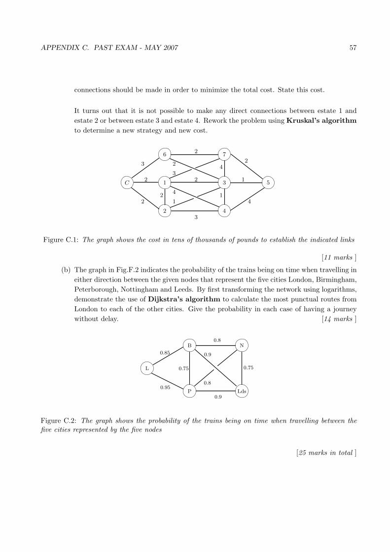
APPENDIX C. PAST EXAM - MAY 2007 57
connections should be made in order to minimize the total cost. State this cost.
It turns out that it is not possible to make any direct connections between estate 1 andestate 2 or between estate 3 and estate 4. Rework the problem using Kruskal’s algorithmto determine a new strategy and new cost.
C
6 7
51 3
2 4
12 1
2
2 2
22
4
4
3
31
2
3
4
Figure C.1: The graph shows the cost in tens of thousands of pounds to establish the indicated links
[11 marks ]
(b) The graph in Fig.F.2 indicates the probability of the trains being on time when travelling ineither direction between the given nodes that represent the five cities London, Birmingham,Peterborough, Nottingham and Leeds. By first transforming the network using logarithms,demonstrate the use of Dijkstra’s algorithm to calculate the most punctual routes fromLondon to each of the other cities. Give the probability in each case of having a journeywithout delay. [14 marks ]
L
B
P
N
Lds0.95
0.9
0.85
0.8
0.75
0.8
0.9
0.75
Figure C.2: The graph shows the probability of the trains being on time when travelling between thefive cities represented by the five nodes
[25 marks in total ]

APPENDIX C. PAST EXAM - MAY 2007 58
Question 4
(a) For a flow problem define the term basic network.
For a basic network:
(i) Write down the conditions that must be satisfied by the flow fi,j from node(i) to node(j).
(ii) With explanation, give an expression for the flow in the network.
[6 marks ]
(b) State the Max-Flow Min-Cut theorem and hence for the network in Fig.D.7 construct bytrial a cut and a flow to establish the maximum flow in the network.
[7 marks ]
A
B E
C
D
F
G
-
-
>
>
~? ?
3
R
~
= R3
3
2
2
2
2
1
1
6
5
7
4
Figure C.3: The numbers indicate the capacities of each arc. The arrows indicate the direction of flowin each arc.
(c) The graph in Fig. D.8 represents a one-way road network taking traffic from point S topoint T in the directions indicated by the arrows and passing through the four roundaboutsR1, R2, R3 and R4. The average maximum capacity of each road is shown on the diagramin terms of vehicles per minute and with the exception of R4 the roundabouts can dealwith all possible flows of traffic. Although the roundabout R4 is scheduled to be updated,at present it can only deal with 20 vehicles per minute.
S
R1 R2
R3
~R4
T
-
-
>
3
~
>
~60
50
50
100
40
30
30
50
Figure C.4: Arrows indicate the direction of traffic flow; numbers indicate the maximum flow invehicles/min for each road.
(i) Redraw the network so that it consist entirely of unrestricted nodes.

APPENDIX C. PAST EXAM - MAY 2007 59
(ii) Demonstrate the application of the Ford-Fulkerson algorithm to the amended graphto establish the maximum flow. Hence determine the maximum flow and the associatedflows on each road.
[12 marks ]
[25 marks in total ]
Question 5
A company has an equipments policy that stipulates that no office computers should be morethan five years old. The value to the company of an individual machine is dependent on itsage; the older machines requiring more hardware and software maintenance and hence slowlybecoming less efficient. The company sets up a temporary office several miles from its base withthe intention of closing it down after three years, at which time all the office equipment will besold off. The computers in this office are initially all three years old and you are asked, usingdynamical programming techniques, to formulate an optimal replacement policy over the nextthree years. Although you should assume that all the computers are replaced at the same timeit may not be the best solution to wait until the computers are five years old before making thereplacement. The following table indicates the annual dependency of the revenue, maintenancecost and resale value in pounds sterling of a computer with respect to time. Additionally thecost of a new computer is £3000.
Age Revenue Maintenance Resalein years cost value
t r(t) c(t) s(t)0 2500 25 −1 2300 40 20002 2200 80 15003 1900 120 12504 1500 180 10005 − − 600
Table C.1: The annual revenue and operating cost relate to a computer which is t years old at thestart of the year. The resale value relates to a computer of t years old.
(i) In the context of a dynamical programming approach using backward recursion, identifythe following:
(a) The four decision stages, i = 1 . . . 4.
(b) The state variable xi at each stage.
(c) The decisions at each stage.
(d) An optimization functional fi(xi) and a defining recursion relation.
[7 marks ]

APPENDIX C. PAST EXAM - MAY 2007 60
(ii) Draw a suitable network to illustrate the above problem, indicating clearly the four stages.Hence use your network, by making suitable annotations at each node, to obtain the optimalstrategy and return for the problem. (Show all your working.)
[18 marks ]
[25 marks in total ]
Question 6
Polycrock is a company making various items of crockery and cutlery out of plastic and polystyrene.Next week the polystyrene cup department is to make exactly 125,000 small sized cups, 80,000medium sized cups and 100,000 large sized cups. The cup department has three machines, M1,M2 and M3, on which to produce the cups. Each machine is capable of producing any size of cupbut can only produce one cup size at any one time. The amount of waste produced in makingeach cup varies from cup size to cup size and machine to machine. Table C.2 gives the amountof waste measured in milligrams per cup for all possible modes of production. The time for
Machine Small Medium Largecup cup cup
M1 25 10 30M2 25 30 10M3 30 35 30
Table C.2: The amount of waste per cup measured in milligrams
each type of machine to produce each type of cup also varies with respect to machine and cup.Table C.3 gives the number of items produced on each machine per minute. The availability
Machine Small Medium Largecup cup cup
M1 40 30 25M2 50 30 20M3 60 50 40
Table C.3: Production rates measured in items per minute
of machine time during the week is 40 hours for machine M1, 40 hours for machine M2 and 45hours for machine M3.
Polycrock wish to know how to schedule the work across the three machines during the comingweek in order to minimize the amount of waste.
For the coming week denote the number of small cups produced on machine Mi by xS,i, thenumber of medium cups produced on machine Mi by xM,i and the number of large cups producedon machine Mi by xL,i where in each case i = 1, 2, 3.

APPENDIX C. PAST EXAM - MAY 2007 61
(a) Formulate the linear programming problem in terms of these nine variables to determinethe optimal production strategy for the coming week. Show clearly the derivation of theconstraints and the objective function.
[9 marks ]
(b) The data in Table C.4 is the computer output from solving the problem. Use this data toanswer the following questions:
(i) What is the optimal strategy and how much waste, expressed in kilograms, is produced?[4 marks ]
(ii) State which constraints are binding and which are not. [2 marks ]
(iii) Three of the shadow prices are positive and three are negative, explain in terms of theproblem why this should be so. [2 marks ]
(iv) If it is possible to increase the available time on just one machine by 30 minutes, whichmachine should this be? Hence calculate the improvement in the objective function inthis case. [2 marks ]
(v) If it is required to produce 1000 more small cups how much more waste is produced?[2 marks ]
(vi) Calculate the feasible range for the number of small cups produced. [2 marks ]
(vii) From the table no small cups are produced on M3. By making the production of smallcups on M3 less wasteful is it possible, within the optimum strategy, to start makingsmall cups on M3? Comment similarly on the production of medium and large cupson M2. [2 marks ]

APPENDIX C. PAST EXAM - MAY 2007 62
Variables
Final Reduced Objective Allowable Allowable
Value Cost Coefficient Increase Decrease
xS,1 5000 0 25 36.25 105.75
xS,2 120000 0 25 105.75 1E+30
xS,3 0 36.25 30 1E+30 36.25
xM,1 26250 0 10 23.81 1E+30
xM,2 0 176.25 30 1E+30 176.25
xM,3 53750 0 35 1E+30 23.81
xL,1 35000 0 30 1E+30 21.75
xL,2 0 401.87 10 1E+30 401.87
xL,3 65000 0 30 21.75 1E+30
Constraints
Final Shadow Constraint Allowable Allowable
Value Price R.H. Side Increase Decrease
Small 125000 493.75 125000 1400.00 2333.33
Med 80000 635.00 80000 1093.75 1750.00
Large 100000 780.00 100000 875.00 1400.00
M1 2400 -18750.00 2400 58.33 35.00
M2 2400 -23437.50 2400 46.67 28.00
M3 2700 -30000.00 2700 35.00 21.88
Objective function
Waste Value
z 8268750
Name
Name
Table C.4: Output from computer solution of Q6. The constraints Small, Med and Large relate to therequirements that a fixed number of different types of cup are to be produced. The constraints M1, M2and M3 relate to the availability of the different types of machine.
[25 marks in total ]

APPENDIX C. PAST EXAM - MAY 2007 63
C.2 Solutions
Solutions May 2007
1. (i) Let y1 denote the number of Regular tablets per week and y2 the number of Extra tabletsper week.Therefore the amount of Vit A/week = 0.1y1 + 0.3y2
and the amount of Vit C/week = 0.2y1 + 0.2y2. Thus to meet the recommended amounts:
0.1y1 + 0.3y2 ≥ 1.7 0.2y1 + 0.2y2 ≥ 1.8 ⇒(
0.1 0.30.2 0.2
)(y1
y2
)≥
(1.71.8
)= c
The total cost of the tablets is given by z = 0.5y1 + 1.2y2 = bT y [5 marks ]
y1
y2
0.1y1 + 0.3y2 = 1.7
0.2y1 + 0.2y2 = 1.8 z = 6 = 0.5y1 + 1.2y2
(5, 4)
0.1x1 + 0.2x2 = 0.5
x1
x2
0.3x1 + 0.2x2 = 1.2
z = 4 = 1.7x1 + 1.8x2
( 72, 3
4)
(a)(b)
Figure C.5: (a): primal minimization problem [3 marks ] (b): Dual maximization problem [3 marks ]
(ii) From Fig.C.5(a) the objective function is minimum at (5, 4). Thus we should buy 5 Regtablets and 4 Extra tablets at a cost of 7.3p/wk. [2 marks ]
(iii) The dual problem is maximize z = cT x = 1.7x1 + 1.8x2 subject to :(
0.1 0.20.3 0.2
)x ≤
(0.51.2
)= b
[2 marks ]In terms of the problem let x1 denote the price in pence per mg of vitamin A and x2 theprice in pence per mg of vitamin C. The manufacturer will try and maximize the cost ofthe recommended weekly supply of vitamins, namely z = 1.7x1 + 1.8x2

APPENDIX C. PAST EXAM - MAY 2007 64
Supplied separately the cost of the vitamins in the Regular tablet is given by 0.1x1 + 0.2x2
which to be competitive with the Regular tablet must cost no more than a Regular tablet.Thus 0.1x1 + 0.2x2 ≤ 0.5
Similarly arguing for the Extra tablet 0.3x1 + 0.2x2 ≤ 1.2 [3 marks ]
(iv) It is required to prove that cT x ≤ bT y, given x ≥ 0, y ≥ 0, c ≤ AT y and Ax ≤ b.
c ≤ AT y ⇒ cT ≤ yT A which, since x ≥ 0 ⇒ cT x ≤ yT Ax ≤ yT b = bT y
[5 marks ]
(v) From FigC.5(b) the maximum is at (72 , 3
4). Since the dual variable x1 is the greater it ismore advantageous for the consumer if the recommended amount of vitamin A is reduced.
[2 marks ]
2. (a) (i) A basic solution is obtained by selecting m independent columns of A, setting all othernon-associated variables equal to zero and solving the m equations in m unknowns.
[2 marks ]
(ii) By inspection col(1) and col(2) independent thus x1 = x2 = 1 and x3 = 0 basic solution.Select the final two columns, set x1 = 0 solve to get x2 = x3 = 1/2Select the first and last columns, set x2 = 0 solve to get x1 = −1, x3 = 1
[3 marks ]
(iii) At most nCm basic solutions. In the simplex method the optimal value occurs at afeasible basic solution thus there are only a finite number of steps to reach the solution.
[2 marks ]
(b) (i) In matrix form:
z = (2, 1, 2,−M, 0, 0)
x1
x2
x3
a1
s1
s2
= cT x Ax =
1 1 1 1 0 04 2 1 0 1 01 1 2 0 0 1
x =
132
= b
[2 marks ]

APPENDIX C. PAST EXAM - MAY 2007 65
(ii)
x1 x2 x3 a1 s1 s2 d rBasic cj 2 1 2 −M 0 0
a1 −M 1 1 1 1 0 0 1 1s1 0 4 2 1 0 1 0 3 [3/4]s2 0 1 1 2 0 0 1 2 2zj −M −M −M −M 0 0 z =
∆zj [2 + M ] 1 + M 2 + M 0 0 0 −M
Table C.5: 2 + M max in final row hence bring in x1 (or x3); 3/4 smallest in final col thus take outs1.
[4 marks ]
(iii)
x1 x2 x3 a1 s1 s2 d rBasic cj 2 1 2 −M 0 0
a1 −M 0 1/2 3/4 1 −1/4 0 1/4 [1/3]x1 2 1 1/2 1/4 0 1/4 0 3/4 3s2 0 0 1/2 7/4 0 −1/4 1 5/4 5/7
zj 2 1− M2 −3M
4 + 12 −M M
4 + 12 0 z =
∆zj 0 M2 [32 + 3M
4 ] 0 −M4 − 1
2 0 −M4 + 3
2
[32 + 3M4 ] max in final row hence bring in x3; [1/3] smallest in final col thus take out s1.
[3 marks ]
x1 x2 x3 a1 s1 s2 d rBasic cj 2 1 2 −M 0 0x3 2 0 2/3 1 4/3 −1/3 0 1/3x1 2 1 1/3 0 −1/3 1/3 0 2/3s2 0 0 −2/3 0 −7/3 1/3 0 2/3zj 2 2 2 2 0 0 z =
∆zj 0 −1 0 −M − 2 0 0 2Final row ≤ 0 thus optimal. [3 marks ]
The optimal solution is x1 = 2/3, x3 = 1/3, x2 = 0 and zmax = 2. [1 mark ]
(iv) To obtain the range of optimality recalculate the last tableau with the x1 coefficientreplaced by α, this only affects the final two rows.

APPENDIX C. PAST EXAM - MAY 2007 66
x1 x2 x3 a1 s1 s2 d rBasic cj α 1 2 −M 0 0x3 2 0 2/3 1 4/3 −1/3 0 1/3x1 α 1 1/3 0 −1/3 1/3 0 2/3s2 0 0 −2/3 0 −7/3 1/3 0 2/3
zj α 43 + α
3 2 83 − α
3 −23 + α
3 0 z =
∆zj 0 −13 − α
3 0 −M − 83 + α
323 − α
3 0 2
To remain optimal α must be such that the final row ≤ 0. [3 marks ]Since −M − 8
3 + α3 is always less than zero, require α such that:
−13− α
3≤ 0,
23− α
3≤ 0 ⇒ 2 ≤ α ⇒ range optimality [2,∞)
[2 marks ]
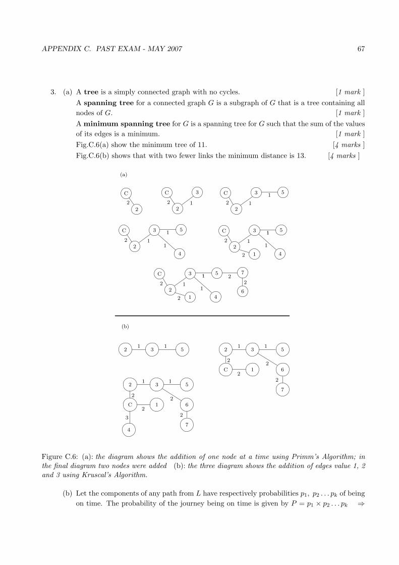
APPENDIX C. PAST EXAM - MAY 2007 67
3. (a) A tree is a simply connected graph with no cycles. [1 mark ]A spanning tree for a connected graph G is a subgraph of G that is a tree containing allnodes of G. [1 mark ]A minimum spanning tree for G is a spanning tree for G such that the sum of the valuesof its edges is a minimum. [1 mark ]Fig.C.6(a) show the minimum tree of 11. [4 marks ]Fig.C.6(b) shows that with two fewer links the minimum distance is 13. [4 marks ]
C
2
C
2
3
2 2 1
C
2
3
2 1
51
C
2
3
2 1
51
1
C
2
3
2 1
51
12 4
1
C
2
3
2 1
51
12 4
1
7
6
22
(a)
4
2 3 51 1
2 3 51 1
C 1 6
7
2
22
2
2 3 51 1
C 1 6
7
2
22
2
4
3
(b)
Figure C.6: (a): the diagram shows the addition of one node at a time using Primm’s Algorithm; inthe final diagram two nodes were added (b): the three diagram shows the addition of edges value 1, 2and 3 using Kruscal’s Algorithm.
(b) Let the components of any path from L have respectively probabilities p1, p2 . . . pk of beingon time. The probability of the journey being on time is given by P = p1 × p2 . . . pk ⇒

APPENDIX C. PAST EXAM - MAY 2007 68
ln(P ) = ln(p1)+ln(p2)+ . . . ln(pk). Since ln pi ≤ 0 consider minimizing − lnP . Hence drawa graph with edge lengths − ln pi. [3 marks ]
Fig.C.7 shows the application of Dijkstra’s method to find the shortest path from L to eachof the other nodes. This enables us to write down the most reliable paths.
London - Birmingham L → B Probability = 0.85
London - Peterborough L → P Probability = 0.95
London - Nottingham L → P → N Probability = 0.95× 0.8 = 0.76
London - Leeds L → P → Lds Probability = 0.95× 0.9 = 0.855 [3 marks ]
L
B
P
N
Lds
0.1625
0.0513
0.2231
0.1054
0.2877
0.1054
0.2231
0.2877
[0, L]
[0.1625, L] [0.4444, Lds]
[0.3856, B]
[0.0513, L]
[0.2744, P ]
[0.1567, P ]
[0.2621, Lds]
[0.3390, P ]
Figure C.7: Nodes labelled [d, n ], where n is the previous node and d is the distance from S. Underlineindicates label is permanent. [8 marks ]

APPENDIX C. PAST EXAM - MAY 2007 69
4. (a) Definition Basic Network: directed graph with at most a single edge between nodes; to eachedge from node(i) to node(j) associate ci,j ≥ 0.; Two special nodes S with no incoming andT with no out going arcs. [2 marks ]
(i) fi,j ≥ 0; fi,j ≤ ci,j ; except for S and T flow into a node = flow out of a node.
[2 marks ]
(ii) The above implies that the total out of S equals the total into T . This amount iscalled the flow of the network and is equal to
∑i fS,i or
∑i fi,T [2 marks ]
(b) Maximum flow in a network is equal to the value of a minimum cut. [1 mark ]
A
B
C
E
F
DG
[1,3]
[1,1]
[1,2]
[6,7]
[5,5]
[0,2]
[0,4]
[1,1]
[0,2]
[1,2]
[0,3]
[6,6]
Figure C.8: Notation [flow, capacity]; value of cut = 7 [3 marks ]; value of flow = 7 [3 marks ]; thusoptimal flow.
(c) The node at R4 is split into two nodes R′4 and R′′
4 with a single link with capacity 20between them. See Fig.C.9(a). [2 marks ]
From Fig.C.9(d) the maximum flow is 110. In terms of the problem the flow from R4 to T
is 20. [2 marks ]

APPENDIX C. PAST EXAM - MAY 2007 70
R1
R3
R2
R′4
T
R′′4
6
-
~
(a)
-
(R2,50)[0, 100]
[0, 40]
-
>
[0, 30]
[60, 60]
[0, 50]
[0.20]
(S,60)
[0, 30]
(R1,50)
-[0, 50]
S
*
~
(S,50)
[0, 50]
[50, 100]
[50, 60]
[50, 50]
R1
R3
R2
R′4
T
R′′4
6
-
~
(b)
-
(R2,40)
[90, 100]
[0, 40]
-
>
[0, 30][0, 50]
[0.20]
(S,10)
[0, 30]
(R3,40)
-[50, 50]
S
*
~
(S,50)
[0, 50]
[50, 100][50, 60]
R1
R3
[40, 50]
[40, 40]
R2
R′4
T
R′′4
6
-
~
(c)
-
(R′′4 ,10)[90, 100]
[40, 40]
-
>
[0, 30][0, 50]
[0.20]
(S,10)
[0, 30]
[40, 50]
-[50, 50]
S
*
~
(S,10)
[50, 60]
[10, 30]
[60, 60]
(R1,10) [10.20] (R′4,10)
[10, 50]
R1
R3
R2
R′4
T
R′′4
6
-
~
(d)
-
(R′′4 ,10)[90, 100]
[40, 40]
-
>
[10, 30][10, 50]
[10.20][0, 30]
[40, 50]
-[50, 50]
S
*
~
(S,10)
[60, 60]
[10, 30]
[50, 50]
(R3,10) [20.20] (R′4,10)
[20, 50]
Figure C.9: Notation: [flow,capacity]; (previous node, max possible increase) [8 marks ]
5. (i) (a) Let i be the start of the ith year [1 mark ]
(b) xi is the age of the machine at the start of ith year. [1 mark ]
(c) Decisions are to Keep or Replace. [1 mark ]
(d) Let fi(xi) be the total revenue from stage i in state xi to the final salvage, i = 1 . . . 4.
fi(xi) = Max{
r(xi)− c(xi) + fi+1(xi + 1) Keepr(0)− c(0) + s(xi)− 3000 + fi+1(1) Replace
}i = 1, 2, 3 f4(x4) = s(x4),
[4 marks ]
(ii) Stage 35−R− 1 2500− 25 + 600− 3000 + 2000 = [2075]
2−R− 1 2500− 25 + 1500− 3000 + 2000 = 29752−K − 3 2200− 80 + 1250 = [3370]
1−K − 2 2300− 40 + 1500 = [3760]1−R− 1 2500− 25 + 2000− 3000 + 2000 = 3475
[4 marks ]
Stage 2

APPENDIX C. PAST EXAM - MAY 2007 71
1−R− 1 2500− 25 + 2000− 3000 + 3760 = 52351−K − 2 2300− 40 + 3370 = [5630]
4−R− 1 2500− 25 + 1000− 3000 + 3760 = [4235]4−K − 5 1500− 180 + 2075 = 3395
[3 marks ]
Stage 13−R− 1 2500− 25 + 1250− 3000 + 5630 = [6355]3−K − 4 1900− 120 + 4235 = 6015
[2 marks ]
In the above the optimal option (max value) is indicated using [] for each decision. Thesevalues are then placed on the relevant node in Fig.C.10.
3
1
4
1
2
5
2
3
1
T
3
j
- -
-
--
*
s-q
3
q~
R
R
R
R
R
K
K
K
K
R
K
(stage 1) (stage 2) (stage 3) (stage 4)x1 x2 x3 x4
[1500,T]
[1250,T]
[2000,T][2075,1]
[3370,3]
[3760,2][5630,2]
[4235,1][6355,1]
Figure C.10: Notation: [fi(xi),next node] [8 marks ]
The return is £6355 per machine with the strategy of Replace, Keep, Keep, Salvage.
[1 mark ]
6. (a) Small cups = 125000 = xs,1 + xs,2 + xs,3 (i)
Medium cups = 80000 = xm,1 + xm,2 + xm,3 (ii)
Small cups = 100000 = xL,1 + xL,2 + xL,3 (iii)
Available time:
M1: 2400 ≥ 140xs,1 + 1
30xm,1 + 125xL,1 (iv)
M2: 2400 ≥ 150xs,2 + 1
30xm,2 + 120xL,2 (v)
M3: 2700 ≥ 160xs,3 + 1
50xm,3 + 140xL,3 (vi)
The constraints are given by (i)− (vi) plus the non-negative condition on all variables.
[7 marks ]
The amount of waste is given by:
z = 25xs,1 + 25xs,2 + 30xs,3 + 10xm,1 + 30xm,2 + 35xm,3 + 30xL,1 + 10xL,2 + 30xL,3
The problem is to minimize this subject to the given constraints. [2 marks ]
(b) (i) Final values of variables give optimal strategy:Small cups: 5000 on M1; 120000 on M2; 0 on M3
APPENDIX C. PAST EXAM - MAY 2007 72
Medium cups: 26250 on M1; 0 on M2; 53750 on M3Large cups: 350000 on M1; 0 on M2; 65000 on M3Waste = 8.269 kg [4 marks ]
(ii) All constraints are binding since RH side=Final Value. [2 marks ]
(iii) If more time is available on a given machine then reschedule to reduce waste - nopoint in changing otherwise - thus expect shadow prices to be negative for the timeconstraints.If we increase the number of cups then we are bound to produce more waste, thus theshadow price for the number of cups expected to be positive. [2 marks ]
(iv) Most negative shadow price for available time is -3000 for M3 thus waste reduced by:30× 3000 = 900g. [2 marks ]
(v) 1000 more small cups increases z by 1000× 493.75 = 493.75g. [2 marks ]
(vi) Feasible range for number of small cups:= [125000− 2333.33, 125000 + 1400] = [122667, 126400]. [2 marks ]
(vii) Waste in producing a small cup on M3 is 30mg. Since the reduced cost for this item is36.25 it is not possible to reduce the amount of waste by this amount.Similarly the reduced costs of the other two processes are greater than the actualamounts of waste already being produced. [2 marks ]
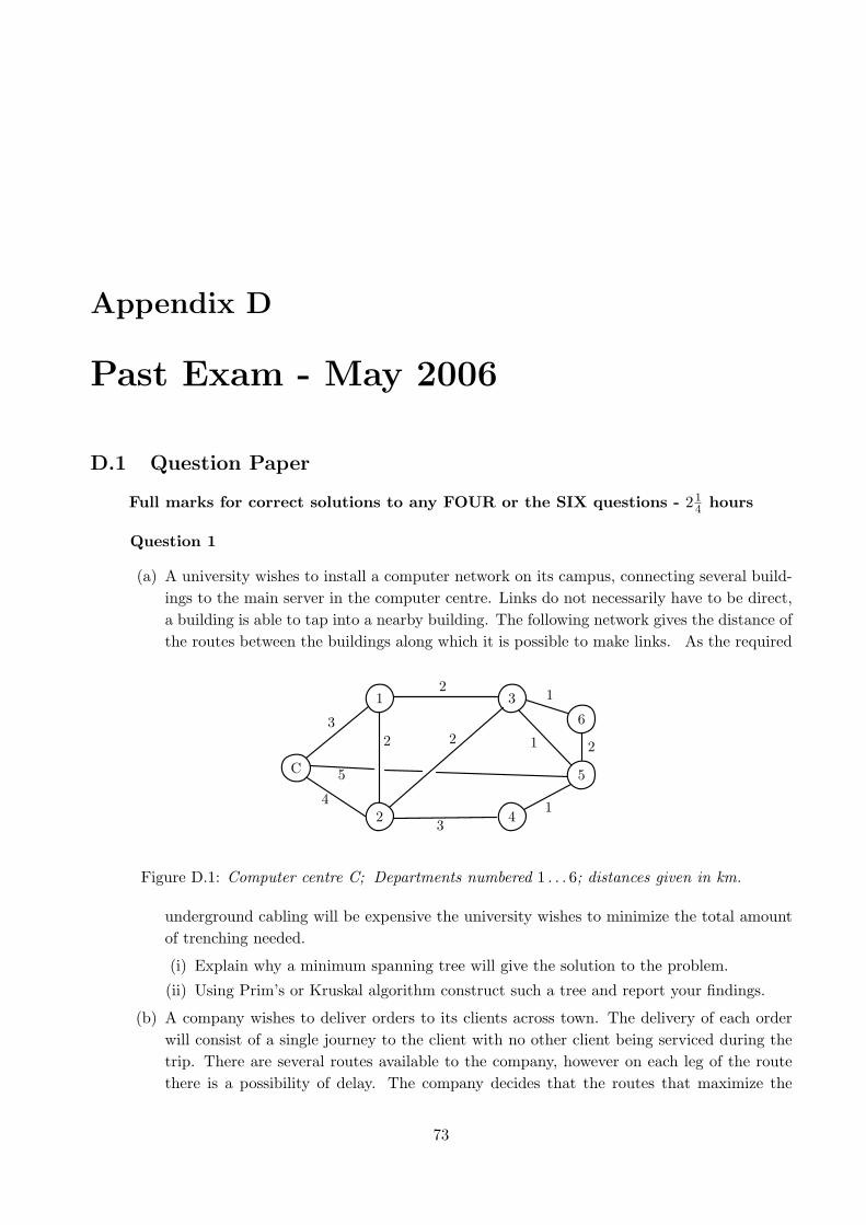
Appendix D
Past Exam - May 2006
D.1 Question Paper
Full marks for correct solutions to any FOUR or the SIX questions - 214 hours
Question 1
(a) A university wishes to install a computer network on its campus, connecting several build-ings to the main server in the computer centre. Links do not necessarily have to be direct,a building is able to tap into a nearby building. The following network gives the distance ofthe routes between the buildings along which it is possible to make links. As the required
C
1
2
3
4
5
63
2
2
5
4
31
21
1
2
Figure D.1: Computer centre C; Departments numbered 1 . . . 6; distances given in km.
underground cabling will be expensive the university wishes to minimize the total amountof trenching needed.
(i) Explain why a minimum spanning tree will give the solution to the problem.
(ii) Using Prim’s or Kruskal algorithm construct such a tree and report your findings.
(b) A company wishes to deliver orders to its clients across town. The delivery of each orderwill consist of a single journey to the client with no other client being serviced during thetrip. There are several routes available to the company, however on each leg of the routethere is a possibility of delay. The company decides that the routes that maximize the
73
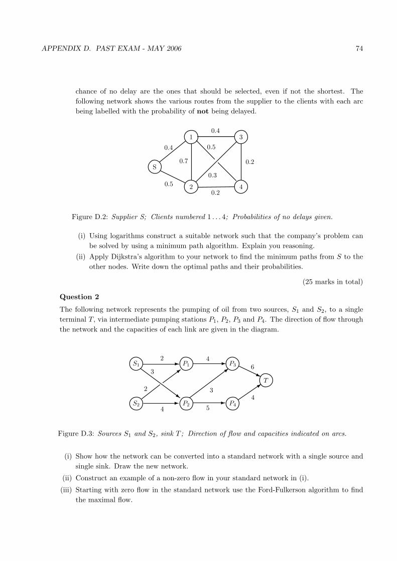
APPENDIX D. PAST EXAM - MAY 2006 74
chance of no delay are the ones that should be selected, even if not the shortest. Thefollowing network shows the various routes from the supplier to the clients with each arcbeing labelled with the probability of not being delayed.
S
1
2
3
4
0.4
0.50.2
0.4
0.20.7
0.3
0.5
Figure D.2: Supplier S; Clients numbered 1 . . . 4; Probabilities of no delays given.
(i) Using logarithms construct a suitable network such that the company’s problem canbe solved by using a minimum path algorithm. Explain you reasoning.
(ii) Apply Dijkstra’s algorithm to your network to find the minimum paths from S to theother nodes. Write down the optimal paths and their probabilities.
(25 marks in total)
Question 2
The following network represents the pumping of oil from two sources, S1 and S2, to a singleterminal T, via intermediate pumping stations P1, P2, P3 and P4. The direction of flow throughthe network and the capacities of each link are given in the diagram.
S1
S2
P1
P2
P3
P4
T
-
~
-
-
3
j>
-
>
46
4
5
3
4
2
3
2
Figure D.3: Sources S1 and S2, sink T ; Direction of flow and capacities indicated on arcs.
(i) Show how the network can be converted into a standard network with a single source andsingle sink. Draw the new network.
(ii) Construct an example of a non-zero flow in your standard network in (i).
(iii) Starting with zero flow in the standard network use the Ford-Fulkerson algorithm to findthe maximal flow.
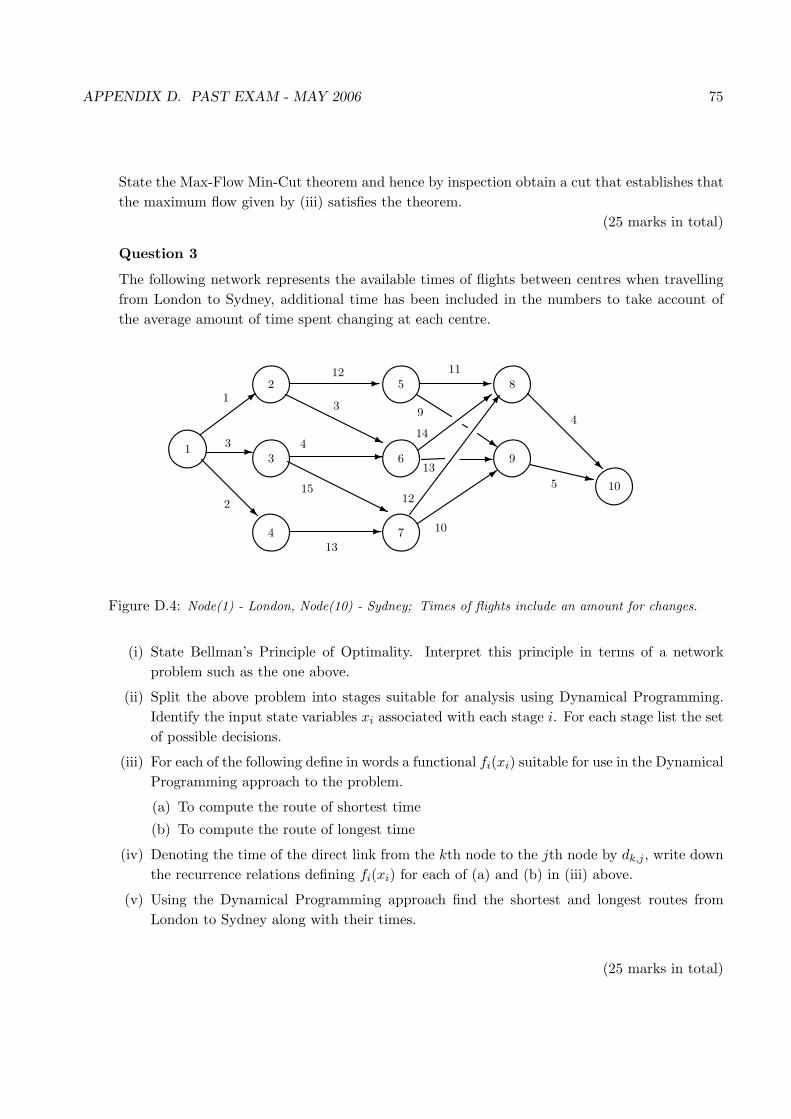
APPENDIX D. PAST EXAM - MAY 2006 75
State the Max-Flow Min-Cut theorem and hence by inspection obtain a cut that establishes thatthe maximum flow given by (iii) satisfies the theorem.
(25 marks in total)
Question 3
The following network represents the available times of flights between centres when travellingfrom London to Sydney, additional time has been included in the numbers to take account ofthe average amount of time spent changing at each centre.
1
2
3
4
5
6
7
8
10
9
>-
j
-
3
j
-
-
7>
4 s-
R
-
1
2
3
12 11
4
Rz
9
5
14
13
12
10
13
15
3
Figure D.4: Node(1) - London, Node(10) - Sydney; Times of flights include an amount for changes.
(i) State Bellman’s Principle of Optimality. Interpret this principle in terms of a networkproblem such as the one above.
(ii) Split the above problem into stages suitable for analysis using Dynamical Programming.Identify the input state variables xi associated with each stage i. For each stage list the setof possible decisions.
(iii) For each of the following define in words a functional fi(xi) suitable for use in the DynamicalProgramming approach to the problem.
(a) To compute the route of shortest time
(b) To compute the route of longest time
(iv) Denoting the time of the direct link from the kth node to the jth node by dk,j , write downthe recurrence relations defining fi(xi) for each of (a) and (b) in (iii) above.
(v) Using the Dynamical Programming approach find the shortest and longest routes fromLondon to Sydney along with their times.
(25 marks in total)

APPENDIX D. PAST EXAM - MAY 2006 76
Question 4
A surveyor visits two types of property, commercial and domestic. Commercial properties takelonger to inspect due to their size and the increased number of health and safety regulations.On average a domestic property takes 10 minutes and a commercial property 40 minutes. Ina given working day the surveyor is not prepared to spend more than five hours per day oninspections and one hour per day in the evenings carrying out the paper work generated by theday’s activities. On average the time to process the paperwork for a domestic property is 3minutes and for a commercial property 7 minutes. Although the surveyor is paid a salary thereis a bonus scheme which pays an extra £3 for each domestic property inspected and £10 foreach commercial property inspected.
Given that there are always properties of each type to inspect and based only on the times tocarry out the inspections and the times to process the paperwork set up the Linear Programmingproblem to calculate how the surveyor should proceed in order to maximize the bonus.
Use graphical means to solve the Linear Programming problem, stating how many types of eachproperty the surveyor should inspect per day and the value of the bonus generated.
Write down the dual problem for the above and hence interpret from the point of view of thesurveyor’s employer.
Solve the dual problem using graphical means.
Use your solution to the dual problem to decide whether or not the surveyor would be betteroff, from the point of view of increasing the bonus, by increasing the number of hours per dayinspecting or by increasing the number of hours per evening doing paperwork.
(25 marks in total)
Question 5
Consider the following problem:
Maximize z = 2x1 + x2 + x3 subject to the constraints:
x1 + x2 ≥ 1, x1 + x2 + 2x3 ≤ 4, x1, x2 , x3 ≥ 0.
(i) Introduce a surplus variable s1, an artificial variable a1, a slack variable s2, and a largeconstant M to write the problem in the augmented matrix form:
Maximize z = cT x, subject to Ax = b, x ≥ 0.
State clearly the values of c, x, b and A.
(ii) Why does the Simplex Method require the extra artificial variable?
(iii) Write down the first Simplex Tableau.
(iv) Find the optimal solution to the problem using the Simplex Method.
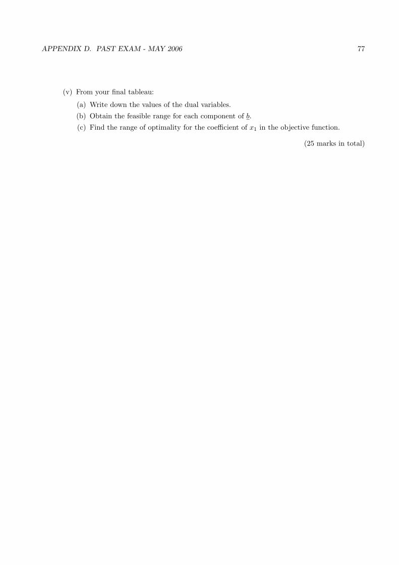
APPENDIX D. PAST EXAM - MAY 2006 77
(v) From your final tableau:
(a) Write down the values of the dual variables.
(b) Obtain the feasible range for each component of b.
(c) Find the range of optimality for the coefficient of x1 in the objective function.
(25 marks in total)

APPENDIX D. PAST EXAM - MAY 2006 78
Question 6
An investment advisor has the following model for investing a client’s funds. The portfolio willcontain shares, unit trusts and cash, with the risk indices and assumed (estimated) annual returnrates given by the following table. The risk index for the portfolio is given by forming the sum
Investment Annual % RiskReturn Rate Index
Shares 12 0.8Unit Trusts 4 0.3
Cash 3 0
Table D.1: Assumed annual returns; Risk indices
of the products of the proportion of each type of investment in the portfolio with its risk index.Thus a portfolio containing 50% shares, 20% unit trusts and 30% cash would have a risk indexof 0.5(0.8)+0.2(0.3)+0.3(0.0)=0.46.
The advisor’s rules for the investment portfolio are:
Rule 1: The portfolio may contain no more than 50% shares.
Rule 2: The amount of investment in unit trusts must be at least half that investedin shares.
Rule 3: The amount of cash must be at least 10% of the total fund.
Rule 4: The amount of cash must be no more than 25% of the total fund.
Let x1 be the proportion of shares, x2 the proportion of unit trusts and x3 the proportion of cashin the portfolio. If the advisor decides to construct a portfolio with risk index of 0.4 write downfour constraining inequalities corresponding to the four rules, one constraint corresponding to thegiven risk index and one final constraint corresponding to the fact that the sum of proportion ofthe products in the portfolio must be one. Express all the constraints with constant non-negativerighthand side.
The objective of the advisor is to maximize the total annual rate of return subject to theconstraints, hence write down the objective function for the problem.
The computer output from the linear programming software is given in Table D.2. Using thisoutput answer the following:
(i) What is the optimal portfolio and its annual return?
(ii) Calculate the feasible range for the righthand side of the constraint for rule 4.
(iii) Is it more beneficial for the advisor to increase the risk by 0.05 or to raise the proportion ofcash invested by ten percentage points? In each case state clearly what the annual returnwould be.
(iv) Explain what is meant by reduced cost and say why in this case they are all zero.
(v) Write down the ranges of optimality for the three objective function coefficients.

APPENDIX D. PAST EXAM - MAY 2006 79
(vi) If the annual rate of return on the unit trusts is taken to be 7% calculate the new optimumannual return on the portfolio. Why is it not possible to carry out this calculation withoutre-running the software if the rate of return is increased to 8%.
Variables
Final Reduced Objective Allowable Allowable
Name Value Cost Coefficient Increase Decrease
x1 0.250 0.000 0.12 1E+30 0.07
x2 0.500 0.000 0.04 0.035 1E+30
x3 0.250 0.000 0.03 1E+30 0.07
Constarints
Final Dual Constraint Allowable Allowable
Name Value Price R.H. Side Increase Decrease Status Slack
Rule 1 0.25 0 0.5 1E+30 0.25 Not Binding 0.25
Rule 2 -0.375 0 0 1E+30 0.375 Not Binding 0.375
Rule 3 0.25 0 0.1 0.15 1E+30 Not Binding 0.15
Rule 4 0.25 0.07 0.25 0.15 0.15 Binding 0
Risk 0.4 0.2 0.4 0.1 0.1 0
Prop 1 -0.04 1 0.25 0.15 0
Value
0.0575
Objective function
Optimal Values
z
Annual Rate
Table D.2: Computer output for Question 6
(25 marks in total)

APPENDIX D. PAST EXAM - MAY 2006 80
D.2 Solutions
Solutions May 2006
Question 1
(a) (i) Need to minimize the total length, connect all nodes, have no redundant loops.[2 marks]
(ii) Use either algorithm to produce Fig. F.1. [4 marks]Total length =10, make the connections as per the diagram. [1 mark]
C 1 2
3 5 4
6
3 2
2
11 1
Figure D.5:
(b) (i) The probability of no delay along a path of length k is given by
P = p1 × p2 × . . . pk
Maximizing P ∼ Maximizing lnP ∼ Maximizing ln p1 + ln p2 + . . . ln pk ∼Minimizing (− ln p1) + (− ln p2) · · ·+ (− ln pk). [3 marks]Thus redraw the network for − ln pi. Fig. F.2 [2 marks]
S
1
2
3
4
0.92
0.69
0.92
0.69
1.61
1.61
1.20
0.36
[S, ∗]
[S, 0.92][2, 1.89]
[2, 2.3][S, 0.69]
[1, 1.84]
[1, 1.61]
Figure D.6: Nodes labelled [n, d ], where n is the previous node and d is the distance from S. Underlineindicates label is permanent.
(ii) · Label S with the permanent label [S, ∗].
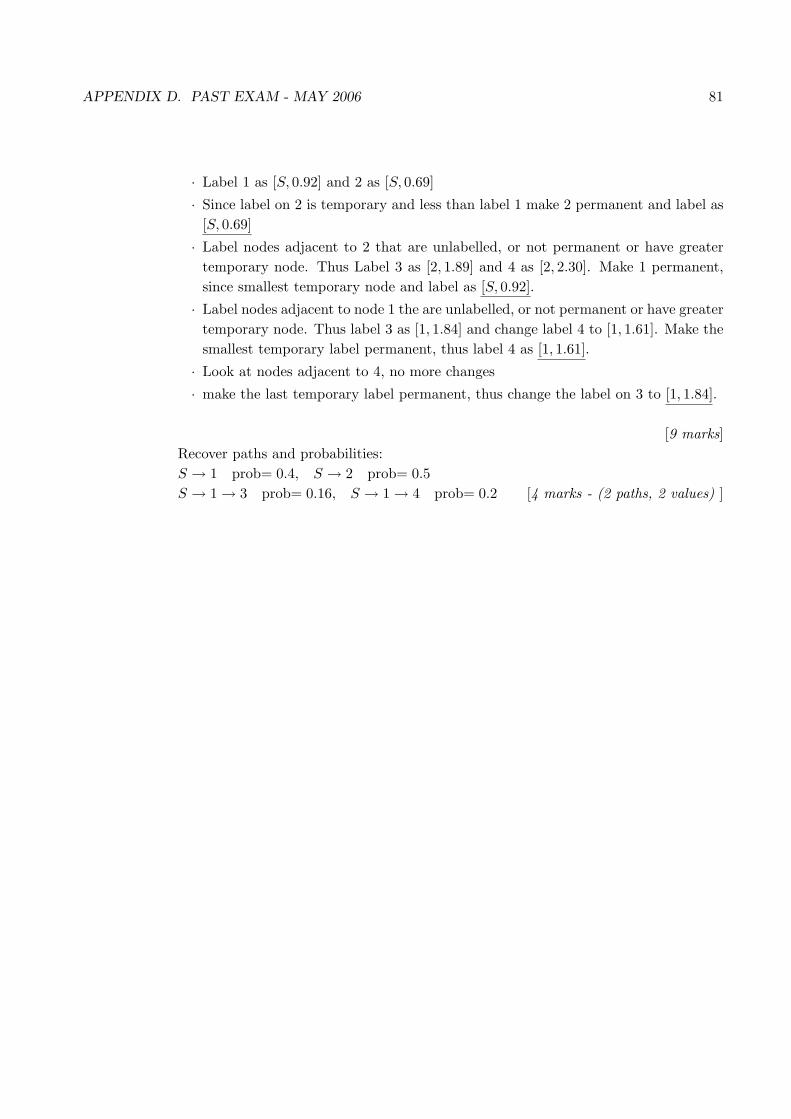
APPENDIX D. PAST EXAM - MAY 2006 81
· Label 1 as [S, 0.92] and 2 as [S, 0.69]
· Since label on 2 is temporary and less than label 1 make 2 permanent and label as[S, 0.69]
· Label nodes adjacent to 2 that are unlabelled, or not permanent or have greatertemporary node. Thus Label 3 as [2, 1.89] and 4 as [2, 2.30]. Make 1 permanent,since smallest temporary node and label as [S, 0.92].
· Label nodes adjacent to node 1 the are unlabelled, or not permanent or have greatertemporary node. Thus label 3 as [1, 1.84] and change label 4 to [1, 1.61]. Make thesmallest temporary label permanent, thus label 4 as [1, 1.61].
· Look at nodes adjacent to 4, no more changes
· make the last temporary label permanent, thus change the label on 3 to [1, 1.84].
[9 marks]Recover paths and probabilities:S → 1 prob= 0.4, S → 2 prob= 0.5S → 1 → 3 prob= 0.16, S → 1 → 4 prob= 0.2 [4 marks - (2 paths, 2 values) ]
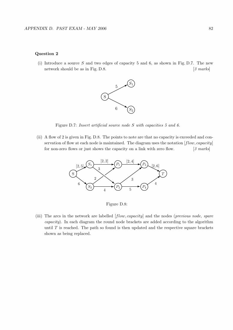
APPENDIX D. PAST EXAM - MAY 2006 82
Question 2
(i) Introduce a source S and two edges of capacity 5 and 6, as shown in Fig. D.7. The newnetwork should be as in Fig. D.8. [3 marks]
S
S1
S2
*
j
5
6
Figure D.7: Insert artificial source node S with capacities 5 and 6.
(ii) A flow of 2 is given in Fig. D.8. The points to note are that no capacity is exceeded and con-servation of flow at each node is maintained. The diagram uses the notation [flow, capacity]for non-zero flows or just shows the capacity on a link with zero flow. [3 marks]
S1
S2
P1
P2
P3
P4
T
-
~
-
-
3
j>
-
>
[2, 4][2, 6]
45
3
4
2
3
[2, 2]
S
*
~
[2, 5]
6
Figure D.8:
(iii) The arcs in the network are labelled [flow, capacity] and the nodes (previous node, sparecapacity). In each diagram the round node brackets are added according to the algorithmuntil T is reached. The path so found is then updated and the respective square bracketsshown as being replaced.

APPENDIX D. PAST EXAM - MAY 2006 83
S1
S2
P1
P2
P3
P4
T
-
~
-
-
3
j>
-
>
[0, 4][0, 6]
[0, 4]
[0.5]
[0, 3]
[0, 4]
[0, 2]
[0, 3]
[0, 2]
S
*
~
[0, 5]
[0, 6]
[2, 5][2, 2] [2, 4]
[2, 6]
(S,∞)
(S, 5) (S1, 2) (P1, 2)
(P3, 2)
(S, 6) (S1, 3) (P2, 3)
(a)
S1
S2
P1
P2
P3
P4
T
-
~
-
-
3
j>
-
>
[2, 4][2, 6]
[0, 4]
[0.5]
[0, 3]
[0, 4]
[0, 2]
[0, 3]
[2, 2]
S
*
~
[2, 5]
[0, 6]
[4, 6][4, 4] [4, 5]
[4, 4]
(S, 3) (S2, 2) (P2, 3)
(P4, 4)
(S, 6) (S2, 4) (P2, 4)
(S,∞)
(b)
Figure D.9: (a) Shows the initial zero flow and the creation of the flow augmenting path S → S1 →P1 → P3 → T which is then updated by 2 units (b) Show the creation of the flow augmenting pathS → S2 → P2 → P4 → T which is augmented by 4 units
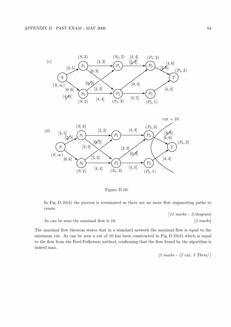
APPENDIX D. PAST EXAM - MAY 2006 84
S1
S2
P1
P2
P3
P4
T
-
~
-
-
3
j>
-
>
[2, 4][2, 6]
[4, 4]
[4, 5]
[0, 3]
[4, 4]
[0, 2]
[0, 3]
[2, 2]
S
*
~
[2, 5]
[6, 6]
[4, 6]
[4, 4]
[4, 6](S, 3) (S2, 2) (P1, 2)
(P3, 2)
(S, 2) (S1, 3) (P2, 1)
(S,∞)
(c)
[2, 2]
S1
S2
P1
P2
P3
P4
T
-
~
-
-
3
j>
-
>
[4, 4]
[6, 6]
[4, 4]
[4, 5]
[0, 3]
[4, 4]
[2, 2]
[0, 3]
[2, 2]
S
*
~
[2, 5]
[6, 6]
[2, 3] [2, 3]
[4, 6][4, 5]
(S, 3) (P2, 3)
(P3, 2)
(S, 2) (S1, 3) (P2, 1)
(S,∞)
(d)
cut = 10
Figure D.10:
In Fig. D.10(d) the process is terminated as there are no more flow augmenting paths tocreate.
[12 marks - 3/diagram]
As can be seen the maximal flow is 10. [2 marks]
The maximal flow theorem states that in a standard network the maximal flow is equal to theminimum cut. As can be seen a cut of 10 has been constructed in Fig. D.10(d) which is equalto the flow from the Ford-Fulkerson method; confirming that the flow found by the algorithm isindeed max.
[5 marks - (2 cut, 3 Thrm) ]

APPENDIX D. PAST EXAM - MAY 2006 85
Question 3
(i) A optimal policy has the property that whatever the initial state and initial decision are, theremaining decisions must constitute an optimal policy with regards to the state resultingfrom the first decision. [2 marks]
In this problem if node(i) is on the optimal path for the problem then using the samecriteria of optimality all the nodes after i are on the optimal path. [3 marks]
(ii) Stage 4 with input {1} and output {2, 3, 4}Stage 3 with input {2, 3, 4} and output {5, 6, 7}Stage 2 with input {5, 6, 7} and output {8, 9}Stage 1 with input {8, 9} and output {10}The state variable xi is the input to stage i [2 marks]
At each stage i choose for input xi one of the elements of Di of the form (xi, ∗) where thedecision sets are given by:
D4 = {(1, 2), (1, 3), (1, 4)} D3 = {(2, 5), (2, 6), (3, 6), (3, 7), (4, 7)}D2 = {(5, 8), (5, 9), (6, 8), (6, 9), (7, 8), (7, 9)} D3 = {(8, 10), (9, 10)} [2 marks]
(iii) (a) Let fi(xi) stand for the shortest distance of the input node xi at stage i to node(10).
(b) Let fi(xi) stand for the longest distance of the input node xi at stage i to node(10).[2 marks]
(iv) (a) fi(xi) = minxi links
{di,i−1 + fi−1(xi−1)} i = 1, . . . 4 x0 = 10, f0(x0) = 0
(b) fi(xi) = maxxi links
{di,i−1 + fi−1(xi−1)} i = 1, . . . 4 x0 = 10, f0(x0) = 0 [4 marks]
(v) Using the notation [total min distance to 10, next node in path] and (total max distanceto 10, next node in path) Fig. D.11 shows the completed network starting from node(10)and working back to node(1).
Shortest path 1 → 2 → 6 → 8 → 10 min distance = 22 [5 marks]
Longest path 1 → 3 → 7 → 8 → 10 max distance = 34 [5 marks ]

APPENDIX D. PAST EXAM - MAY 2006 86
1
2
3
4
5
6
7
8
10
9
>-
j
-
3
j
-
-
7>
4 s-
R
-
1
2
3
12 11
4
Rz
9
5
14
13
12
1013
15
3
(27,5) (15,8) (4,10)
(5,10)
(16,8)(29,7)
(34,3)(31,7) (18,8)
[21,6] [14,9] [4,10]
[5,10]
[28,7] [15,9]
[22,2] [22,6] [18,8]
Figure D.11:
Question 4
Linear Programming Problem [5 marks ]
Let x1 ≥ 0 be the number of domestic dwellings inspected and x2 ≥ 0 the number ofdomestic dwelling inspected per day.
The constraint for the time to inspect is 10x1 + 40x2 ≤ 300
The constraint for the time to do the associated paperwork is 3x1 + 7x2 ≤ 60
Bonus for doing the inspections z = 3x1 + 10x2
Solution
Diagram Fig. D.12(a) [2 marks ]
Verify that the max is at P with x1 = x2 = 6 and z = £78. [2 marks ]
Dual Problem
Minimize z = 300y1 + 60y2 subject to:
10y1 + 3y2 ≥ 3 40y1 + 7y2 ≥ 10, y1, y2 ≥ 0 [5 marks ]
Interpretation of Dual
y1 is the amount of bonus paid per minute for carrying out inspections.
y2 is the amount of bonus paid per minute for doing the paperwork

APPENDIX D. PAST EXAM - MAY 2006 87
B
P
A20 30
7.5
x1 + 4x2 = 30
3x1 + 7x2 = 60
x1
x2
Oy1
y2
(a) (b)
A
B
P
0.30.25
110y1 + 3y2 = 3
40y1 + 7y2 = 10
O
Figure D.12: (a) Primal problem (b) Dual problem
Company would like to minimize the amount of bonus earned in a day, that is to sayminimize z = 300y + 60y2.However they will still need to pay at least £3 per domestic inspection and £10 percommercial inspection. Thus:
domestic 10y1 + 3y2 ≥ 3 commercial 40y1 + 7y2 ≥ 10
[5 marks ]
Solution of Dual
The solution to the dual problem is given in Fig. D.12(b) [2 marks ]
Verify that the min is at P with: y1 = 950 , y2 = 2
5 and z = £78. [2 marks ]
The dual solutions are the shadow or dual prices of the primal problem. Since y2 > y1
it is therefore more beneficial for the surveyor to allocate more time to paperwork.[2 marks ]
Question 5
(i) Introducing the extra variables:
x1 + x2 − s1 + a1 = 1 x1 + x2 + 2x3 + s2 = 4 z = 2x1 + x2 + x3 −Ma1
Thus:
A =(
1 1 0 −1 1 01 1 2 0 0 1
)b =
(14
)cT = (2, 1, 1, 0,−M, 0) xT = (x1, x2, x3, s1, a1, s2)
[3 marks ]
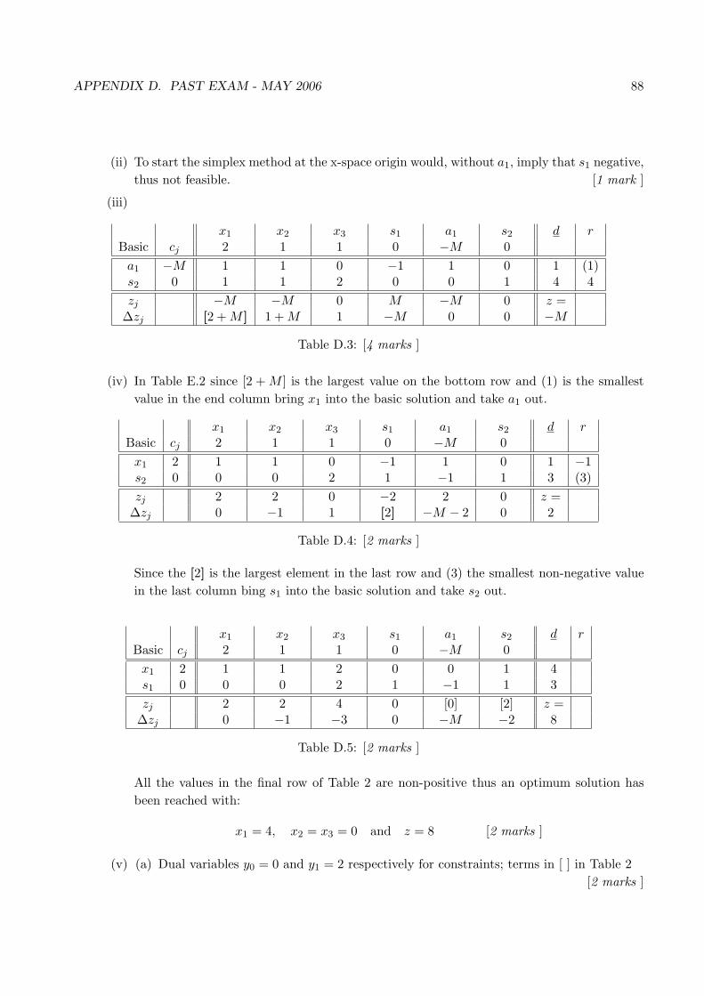
APPENDIX D. PAST EXAM - MAY 2006 88
(ii) To start the simplex method at the x-space origin would, without a1, imply that s1 negative,thus not feasible. [1 mark ]
(iii)
x1 x2 x3 s1 a1 s2 d rBasic cj 2 1 1 0 −M 0
a1 −M 1 1 0 −1 1 0 1 (1)s2 0 1 1 2 0 0 1 4 4zj −M −M 0 M −M 0 z =
∆zj [2 + M ] 1 + M 1 −M 0 0 −M
Table D.3: [4 marks ]
(iv) In Table E.2 since [2 + M ] is the largest value on the bottom row and (1) is the smallestvalue in the end column bring x1 into the basic solution and take a1 out.
x1 x2 x3 s1 a1 s2 d rBasic cj 2 1 1 0 −M 0x1 2 1 1 0 −1 1 0 1 −1s2 0 0 0 2 1 −1 1 3 (3)zj 2 2 0 −2 2 0 z =
∆zj 0 −1 1 [2] −M − 2 0 2
Table D.4: [2 marks ]
Since the [2] is the largest element in the last row and (3) the smallest non-negative valuein the last column bing s1 into the basic solution and take s2 out.
x1 x2 x3 s1 a1 s2 d rBasic cj 2 1 1 0 −M 0x1 2 1 1 2 0 0 1 4s1 0 0 0 2 1 −1 1 3zj 2 2 4 0 [0] [2] z =
∆zj 0 −1 −3 0 −M −2 8
Table D.5: [2 marks ]
All the values in the final row of Table 2 are non-positive thus an optimum solution hasbeen reached with:
x1 = 4, x2 = x3 = 0 and z = 8 [2 marks ]
(v) (a) Dual variables y0 = 0 and y1 = 2 respectively for constraints; terms in [ ] in Table 2[2 marks ]

APPENDIX D. PAST EXAM - MAY 2006 89
(b) For b1:(
43
)+ δ
(0−1
)≥ 0 ⇒ δ ≤ 3 ⇒ b1 ∈ (−∞, 4] [2 marks ]
For b2:(
43
)+ δ
(11
)≥ 0 ⇒ δ ≥ −3 ⇒ b2 ∈ [1,∞) [2 marks ]
(c) To investigate the range of optimality for x1 replace the coefficient of x1 in the objectivefunction with α in the final tableau. This gives Table E.5 from which:
x1 x2 x3 s1 a1 s2 d rBasic cj α 1 1 0 −M 0x1 α 1 1 2 0 0 1 4s1 0 0 0 2 1 −1 1 3zj α α 2α 0 0 α z =
∆zj 0 1− α 1− 2α 0 −M −α 4α
Table D.6: [3 marks ]
For the solution to remain optimal the final row must remain non-positive, thus:
1− α ≤ 0 1− 2α ≤ 0 − α ≤ 0 ⇒ 1 ≤ α
Thus the range of optimality is [1,∞). [2 marks ]
Question 6
The inequality constraints are:
x1 ≤ 0.5 x2 − x1
2≥ 0 x3 ≥ 0.1 x3 ≤ 0.25
The equation constraints are:
(risk) 0.8x1 + 0.3x2 = 0.4 (sum=1) x1 + x2 + x3 = 1
Objective function to maximize the rate of return
z = 0.12x1 + 0.04x2 + 0.03x3
Variables non-negative. [7 marks ]
(i) From the data x1 = x3 = 0.25 and x2 = 0.5.
Thus investment is: 50% unit trust 25% cash and 25% shares
Annual return is 5.75% [3 marks ]

APPENDIX D. PAST EXAM - MAY 2006 90
(ii) From the data the change in rhs rule4 is ±0.15 Thus the feasible range for the righthandside of rule4 is given by:
0.25− 0.15 ≤ rhs ≤ 0.25 + 0.15 ⇒ [0.1, 0.4]
[2 marks ]
(iii) Dual price for Risk = 0.2 thus increase in z due to an increase of 0.05 is = 0.2 × 0.05 =0.01 ⇒ Return = 6.75%.
Dual price of investing cash = 0.07 thus the increase in z due to an increase of 10% points,that is to say 0.1, is 0.007 ⇒ Return = 6.45%
Thus increase the level of risk. [4 marks ]
(iv) Reduced cost of a particular variable is the change in the corresponding coefficient in theobjective function such that there exists an optimal solution with the value of this variablenon-zero. If the variables are already non-zero at the optimal solution, as in this examplethen no changes are needed and hence all the reduced costs are zero. [2 marks ]
(v) If z = 0.12x1 + 0.04x2 + 0.03x3 = c1x1 + c2x2 + c3x3 then the data gives the possibleincreases and decreases of ci.
c1 : 0.12− 0.07 ≤ c1 < ∞ ⇒ [0.05,∞)
c2 : −∞ < c2 ≤ 0.04 + 0.035 ⇒ (−∞, 0.075]
c3 : 0.03− 0.07 ≤ c3 < ∞ ⇒ [−0.04,∞) [3 marks ]
(vi) 7%=0.07 is inside the range of optimality for c2 thus the solution is still valid and thus thenew value of z given by:
z = 0.25× 0.12 + 0.5.07 + 0.25× 0.03 = 0.0725 = 7.25% [3 marks ]
8%=0.08 is outside the optimal range for c2 thus the problem would need to be resolved.[1 mark ]

Appendix E
Specimen Exam Type Questions andSolutions
E.1 Specimen Questions
The following questions are intended to give you an idea of the type of problem I will expect you tobe able to solve. In the exam the the problems are balanced to be all about the same length, in thefollowing this is not the case. That is to say some of the following problems will be shorter and somelonger than those found in the exam
E.1.1 Minimal spanning tree problem
A spanning tree links all nodes in a network and has no cycles. Associating a positive value with eachedge of the network gives the idea of a minimum spanning tree. Such a tree is therefore the mosteconomical arrangement, in terms of the associated edge values, for connecting all nodes.
E
1 2 3 4
5 6 7 8
9 10
2
1 6 2
3
41
2
3
5
1
4
12
3
Figure E.1:
1. Figure E.1 gives the layout of all possible routes for telephone links between the main exchangeE and local substations (distances in km). All substations need to be linked to E either directlyor via another substation.
91

APPENDIX E. SPECIMEN EXAM TYPE QUESTIONS AND SOLUTIONS 92
Since the links are to be underground find the layout that involves the least amount of tunnelling.(That is find the minimum spanning tree for the network).
(a) Using Prim’s algorithm
(b) Using Kruskal’s algorithm
Give the value of the minimum spanning tree.
2. Using either method find the minimum spanning trees for each of the networks in Figure E.2.
(a) (b)
1
2
3
4
5
6
2
14 5
214
3
11
2
3
4 5
6
7
1
1 14
42
2
2
35
Figure E.2:
In each case try and produce two minimum spanning trees, hence verifying that the minimumvalue is unique.
E.1.2 Shortest distance problem
Given a network, to which a positive value is assigned to each edge, we considered two algorithmsthat found the shortest path through the network. In the case of Dijkstra’s algorithm the shortestpaths from a given node to all the other nodes is calculated whereas Floyd’s algorithm calculatesthe shortest path between each pair of nodes. The choice of algorithm depends on the problem athand, if indeed we do only require the shortest path from a given node then Dijkstra’s algorithmis the obvious choice. Floyd’s algorithm is longer but much shorter than applying Dijkstra’salgorithm to each node in turn. In our examples the networks were either mixed or directed,this will tend to be the case in these problems.
3. DijkstraFor each of the networks in Figure E.3 find the shortest paths and their values from the node S
to each of the other nodes. Note that (a) is a directed network whereas (b) is a mixed network.This does not affect the algorithm but you need to keep this in mind when, in the algorithm,you are looking at the nodes directly connected to the last permanent node created.
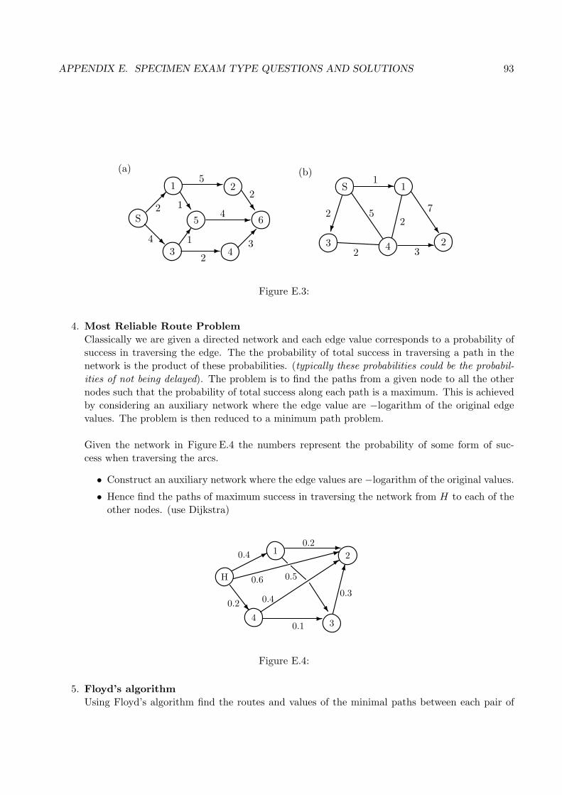
APPENDIX E. SPECIMEN EXAM TYPE QUESTIONS AND SOLUTIONS 93
(a) (b)
S
1
3 4
5 6
2
2µ
^
R7
-
-
^
-µ4
5
2
14
31
1
23 4
1
52
2
2
3
72
S -
^-
°
Figure E.3:
4. Most Reliable Route ProblemClassically we are given a directed network and each edge value corresponds to a probability ofsuccess in traversing the edge. The the probability of total success in traversing a path in thenetwork is the product of these probabilities. (typically these probabilities could be the probabil-ities of not being delayed). The problem is to find the paths from a given node to all the othernodes such that the probability of total success along each path is a maximum. This is achievedby considering an auxiliary network where the edge value are −logarithm of the original edgevalues. The problem is then reduced to a minimum path problem.
Given the network in Figure E.4 the numbers represent the probability of some form of suc-cess when traversing the arcs.
• Construct an auxiliary network where the edge values are −logarithm of the original values.
• Hence find the paths of maximum success in traversing the network from H to each of theother nodes. (use Dijkstra)
1 2
34
H
*-:3
º
-w ^
0.40.2
0.3
0.1
0.40.2
0.6 0.5
Figure E.4:
5. Floyd’s algorithmUsing Floyd’s algorithm find the routes and values of the minimal paths between each pair of
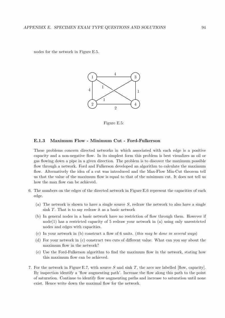
APPENDIX E. SPECIMEN EXAM TYPE QUESTIONS AND SOLUTIONS 94
nodes for the network in Figure E.5.
1
2
3
4
4
4
2
11
1
Figure E.5:
E.1.3 Maximum Flow - Minimum Cut - Ford-Fulkerson
These problems concern directed networks in which associated with each edge is a positivecapacity and a non-negative flow. In its simplest form this problem is best visualizes as oil orgas flowing down a pipe in a given direction. The problem is to discover the maximum possibleflow through a network. Ford and Fulkerson developed an algorithm to calculate the maximumflow. Alternatively the idea of a cut was introduced and the Max-Flow Min-Cut theorem tellus that the value of the maximum flow is equal to that of the minimum cut. It does not tell ushow the max flow can be achieved.
6. The numbers on the edges of the directed network in Figure E.6 represent the capacities of eachedge.
(a) The network is shown to have a single source S, redraw the network to also have a singlesink T . That is to say redraw it as a basic network
(b) In general nodes in a basic network have no restriction of flow through them. However ifnode(1) has a restricted capacity of 5 redraw your network in (a) using only unrestrictednodes and edges with capacities.
(c) In your network in (b) construct a flow of 6 units. (this may be done in several ways)
(d) For your network in (c) construct two cuts of different value. What can you say about themaximum flow in the network?
(e) Use the Ford-Fulkerson algorithm to find the maximum flow in the network, stating howthis maximum flow can be achieved.
7. For the network in Figure E.7, with source S and sink T , the arcs are labelled [flow, capacity].By inspection identify a ’flow augmenting path’. Increase the flow along this path to the pointof saturation. Continue to identify flow augmenting paths and increase to saturation until noneexist. Hence write down the maximal flow for the network.

APPENDIX E. SPECIMEN EXAM TYPE QUESTIONS AND SOLUTIONS 95
1
2
3
4-
-3
jS
34
7
3
2
5s4
Figure E.6:
1
2
3
4-
-
+ jS
3[1,4]
[2,4]
[1,3]
T[1,3]
[2,4]s[0.5]
~
3
[1,3]
[0,3]
Figure E.7:
8. Apply the Ford-Fulkerson algorithm to the network in Figure E.8 to find the maximal flow andshow how it is achieved.
1
2
3
4-
-
+ j
S
3
[0,5]
[0,7]
[0,9]
T[0,3]
s[0.6]
5
6
[0,5]
ª -R
-
s
>
[0,4]
[0,6]
[0,5][0,3]
[0,8]
[0.6]
Figure E.8:
E.1.4 Dynamic Programming
The methodology of Dynamic Programming requires that the problem is split into stages witheach stage having input and output. The input and output variables are called the state variablesfor the system. At each stage a decision is made using an optimal policy. Bellman’s principle

APPENDIX E. SPECIMEN EXAM TYPE QUESTIONS AND SOLUTIONS 96
is used to create a sequence of decisions that usually involves maximizing or minimizing anoptimization functional which is defined via a recurrence relation.
9. The network in Figure E.9 represents possible routes between towns for a journey from town S
to town T . Using the methodology of Dynamic Programming find:
(i) The shortest path from S to T
(ii) The path from S to T that minimizes the longest leg on the route. (Such a path wouldbe of interest if for some reason a person did not wish to travel in a single step more thannecessary even at the expense of a longer journey.)
First however carry out the following:
• Identify suitable stages for the dynamic programming process
• The decision sets Di at each stage.
• The state variables for each stage.
• The recurrence relation for the optimization functional for each of (i) and (ii)
S
2
1
3
4
5
6
8
7
9
10
11
T
µ
1
z
R
s-
-3
*
j
Á
q
j
*
q:
:
q
j*
34
2
4
2
2
12
4
3
6
65
5
2
6
5
3
2
4
Figure E.9:
10. PhotoShop is to develop an equipment replacement policy over the next three years for its supercolour printer. The cost of a new printer is £ 25,000 and the companies policy is to not run aprinter that is more than five years old.
As the printer ages its ability to generate revenue decreases (due mainly from it being downfor repair and the clearing of paper jams ) and the cost of the maintenance contract increases.Table 2gives the annual revenue r(t) and maintenance cost c(t) for a machine that is t years oldat the start of the year. Also the table gives the trade in value s(t) of a machine that is t yearsold.

APPENDIX E. SPECIMEN EXAM TYPE QUESTIONS AND SOLUTIONS 97
Age of Machine Revenue Operating Cost Trade in Valuet years r(t) c(t) s(t)
0 15 1 −1 14 1.2 192 12 1.4 143 9 1.7 114 5 2.1 95 − − 7
Table E.1: Costs in thousands of pounds sterling.
Using the ideas of Dynamical Programming:
• Construct a network to define the problem. Identify the stages, state variables and decisions.Define a suitable optimization functional fi and hence write out the recurrence relationdefining each fi.
• Assuming the shop starts with a three year old printer, obtain the optimal policy for thisproblem over the three year period. The trade in value at the end of the period should beconsidered as a contribution to the total revenue.
11. Simple Knapsack ProblemA cargo ship can carry up to 6 tons of cargo and is to be loaded with one or more of three typesof cargo. The weights in tons and return in thousands of pounds on one item of each cargo typeis given in Table E.2.
cargo weight returntype i tons wi per item ri
1 3 302 4 503 1 15
Table E.2: Weight in tons per item for each type of cargo; profit per item of each type.
Using the knapsack problem from dynamic programming find how best to load the ship in orderto maximize return. That is to say how many items of each type should be loaded to give amaximum return; what is this return.

APPENDIX E. SPECIMEN EXAM TYPE QUESTIONS AND SOLUTIONS 98
E.1.5 Linear Programming
The following problems illustrate the types of problem we have covered. The two dimensionalproblems can be solved using a graph. For problems with more than two dimensions the questionmay ask you to derive the constraints and objective function and then give you the solution inthe form of an Excel report, as seen in the class problems and coursework. Finally the solutionusing the simplex method and the use of the final tableau to investigate the problem will betested, as seen in the final coursework and notes.
12. Using graphical means solve the following linear programming problem.
Maximize z = 3x1 + 2x2 subject to:
x1 + x2 ≤ 3 (i) x1 + 2x2 ≤ 4, 2x1 + x2 ≤ 4 x1, x2 ≥ 0
• Which constraints are binding
• If (i) is replaced with x1 + x2 ≤ 3 + δ with δ ≥ 0 such that the same constraints remainbinding, calculate ∆z
δ , where ∆z is the change in z due to the introduction of δ. In thetheory of linear programming what is this quantity referred to.
13. Using graphical means solve the following linear programming problem.
Maximize z = 3x1 + 2x2 subject to:
x1 + x2 ≤ 3 2x1 + x2 ≤ 4 x1, x2 ≥ 0
• Write down the dual of the problem.
• Use graphical means to solve the dual problem
14. City University pay me separately to work in each of the two departments, Mathematics andActuarial Science. For every one hour lecture I give in the Mathematics Department I am paid£5 and for every one hour lecture I give in the Department of Actuarial Science I am paid £7.Unfortunately each lecture generates extra preparatory work, those in mathematics taking anextra 1hr per lecture and those in Actuarial Science an extra 11
2hrs per lecture. In any given weekI am not prepared to give more than 15hrs lectures or spend more than 19hrs on preparation.How should I best arrange my time between the two departments in order to maximize myreturn. (Solve using a graph)
Write down the dual problem and solve graphically. Interpret the dual problem from the pointof view of City University as an employer.
15. Given
x1
(12
)+ x2
( −11
)+ x3
(21
)=
(41
)
obtain all three sets of basic solutions to the problem. Which, if any, of these sets would be afeasible basic solution for a standardized linear programming problem?

APPENDIX E. SPECIMEN EXAM TYPE QUESTIONS AND SOLUTIONS 99
It is not necessary to use row reduction. You can see that any pair of columns on the left handside are independent, hence in turn, set the other variable equal to zero and solve the simplesimultaneous equations in two variables
16. Use the Simplex Method to Maximize z = 2x1 + x2 + x3 subject to
x1 + x2 + x3 ≤ 4, x1 − 2x2 + x3 ≤ 3 x1, x2, x3 ≥ 0
From the optimal table:
• Write down the dual variables.
• Calculate the range of optimality for the coefficients in the objective function.
• Calculate the feasible range for the righthand sides of the two constraints.
• Write down the dual problem and hence write down its optimal solution.
• Verify your result by solving the dual problem graphically.
17. Consider the problem: Maximize z = 2x1 + x2 subject to
x1 + x2 ≤ 4, x1 + 2x2 ≥ 6 x1, x2 ≥ 0
• Introduce a slack, surplus and artificial variable to write the constraints in a form suitablefor solution by the Simplex Method.
• Introducing a large positive constant M write down a suitable objective function for use inthe Simplex Method
• Solve the problem using the Simplex Method
• Write down the dual variables.
• Calculate the range of optimality for the coefficients in the objective function.
• Calculate the feasible range for the righthand sides of the two constraints.
18. A firm makes three different types of confectionary, milk chocolate, plain chocolate and toffee.The production line consists of five departments (a) - (e). The amount of time taken to processone tonne (1000 kg) of each of the three types in each of the five departments is given in Table E.3.Additionally the total number of hours available in each department during the next week isgiven in the final column of the table. The profit on 1kg of milk chocolate is £1.25, the profiton 1kg of plain chocolate is £1.50 and on 1kg of toffee is £0.75.
Write down the constraints in this problem for production over the next week and the objectivefunction used to maximize the profit.
The output from solving this problem using Solver is given at the end of this question, use thisdata to:
• Write down the optimum production plan and the maximum profit obtained.
• In which department is it most advantageous to increase the available time by a smallamount. What is the maximum amount by which this department could be expanded.
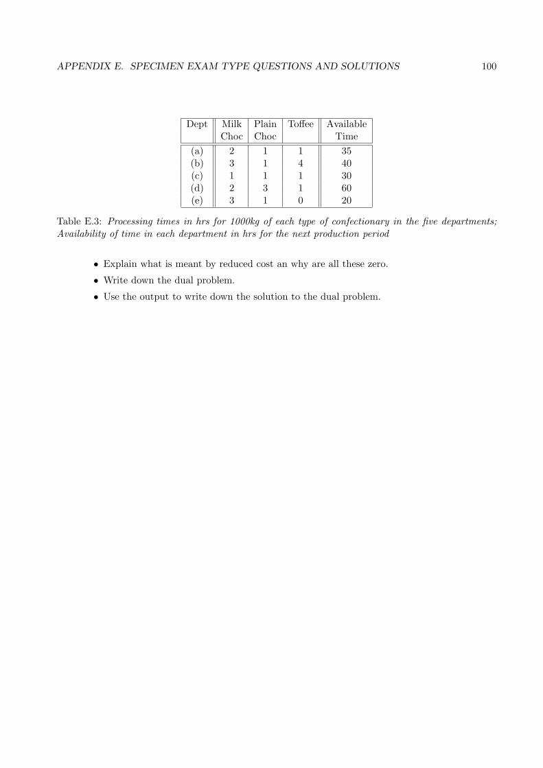
APPENDIX E. SPECIMEN EXAM TYPE QUESTIONS AND SOLUTIONS 100
Dept Milk Plain Toffee AvailableChoc Choc Time
(a) 2 1 1 35(b) 3 1 4 40(c) 1 1 1 30(d) 2 3 1 60(e) 3 1 0 20
Table E.3: Processing times in hrs for 1000kg of each type of confectionary in the five departments;Availability of time in each department in hrs for the next production period
• Explain what is meant by reduced cost an why are all these zero.
• Write down the dual problem.
• Use the output to write down the solution to the dual problem.

APPENDIX E. SPECIMEN EXAM TYPE QUESTIONS AND SOLUTIONS 101
Name Original Value Final Value
z 3500 31429
Adjustable Cells
Name Original Value Final Value
Milk 1.000 0.714
Plain 1.000 17.857Toffee 1.000 5.000
Constraints
Name Cell Value Formula Status Slack
(a) 24.29 $C$3<=$B$3 Not Binding 10.714
(b) 40.00 $C$4<=$B$4 Binding 0.000
( c) 23.57 $C$5<=$B$5 Not Binding 6.429
(d) 60.00 $C$6<=$B$6 Binding 0.000(e) 20.00 $C$7<=$B$7 Binding 0.000
Adjustable Cells
Final Reduced Objective Allowable Allowable
Name Value Cost Coefficient Increase Decrease
Milk 0.71 0.000 1250 3250.00 90.909
Plain 17.86 0.000 1500 200.00 1083.333Toffee 5.00 0.000 750 142.86 285.714
Constraints
Final Shadow Constraint Allowable Allowable
Name Value Price R.H. Side Increase Decrease
(a) 24.29 0.000 35 1E+30 10.714
(b) 40.00 71.429 40 36 20.000
( c) 23.57 0.000 30 1E+30 6.429
(d) 60.00 464.286 60 5 41.667(e) 20.00 35.714 20 20 1.818
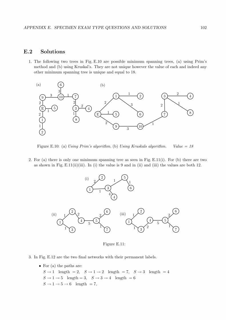
APPENDIX E. SPECIMEN EXAM TYPE QUESTIONS AND SOLUTIONS 102
E.2 Solutions
1. The following two trees in Fig. E.10 are possible minimum spanning trees, (a) using Prim’smethod and (b) using Kruskal’s. They are not unique however the value of each and indeed anyother minimum spanning tree is unique and equal to 18.
E
1 2 3 4
5 6 7 8
9 10
2
1 2
3
1
2
31
12
2
1
E
9 10
6
7
3 4
8
5
1
2
2
1
33
1
2
1
2
(a) (b)
Figure E.10: (a) Using Prim’s algorithm. (b) Using Kruskals algorithm. Value = 18
2. For (a) there is only one minimum spanning tree as seen in Fig. E.11(i). For (b) there are twoas shown in Fig. E.11(ii)(iii). In (i) the value is 9 and in (ii) and (iii) the values are both 12.
(i)
(ii)
1
2
3
4
5
6
1
1
2
3
2
14
4 5
1
6
7
1
1 1
2 2
5
(iii)
1
2
3
4 5
6
7
1
1 12
2
5
Figure E.11:
3. In Fig. E.12 are the two final networks with their permanent labels.
• For (a) the paths are:S → 1 length = 2, S → 1 → 2 length = 7, S → 3 length = 4S → 1 → 5 length = 3, S → 3 → 4 length = 6S → 1 → 5 → 6 length = 7,
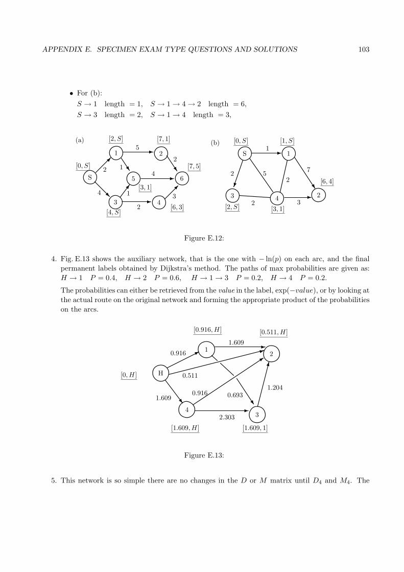
APPENDIX E. SPECIMEN EXAM TYPE QUESTIONS AND SOLUTIONS 103
• For (b):S → 1 length = 1, S → 1 → 4 → 2 length = 6,S → 3 length = 2, S → 1 → 4 length = 3,
(a) (b)
S
1
3 4
5 6
2
2µ
^
R7
-
-
^
-µ4
5
2
14
31
1
23 4
1
52
2
2
3
7
2S -
^-
°
[0, S]
[2, S] [7, 1]
[7, 5]
[6, 3][4, S]
[3, 1]
[0, S] [1, S]
[6, 4]
[3, 1][2, S]
Figure E.12:
4. Fig. E.13 shows the auxiliary network, that is the one with − ln(p) on each arc, and the finalpermanent labels obtained by Dijkstra’s method. The paths of max probabilities are given as:H → 1 P = 0.4, H → 2 P = 0.6, H → 1 → 3 P = 0.2, H → 4 P = 0.2.
The probabilities can either be retrieved from the value in the label, exp(−value), or by looking atthe actual route on the original network and forming the appropriate product of the probabilitieson the arcs.
12
34
H
*-:3
º
-w ^
0.916
1.609
1.204
2.303
0.9161.609
0.511
0.693
[0,H]
[0.916,H] [0.511,H]
[1.609, 1][1.609,H]
Figure E.13:
5. This network is so simple there are no changes in the D or M matrix until D4 and M4. The

APPENDIX E. SPECIMEN EXAM TYPE QUESTIONS AND SOLUTIONS 104
final matrices are given in Eq(F.1).
D4 =
∗ 3 2 13 ∗ 1 22 1 ∗ 11 2 1 ∗
M4 =
1 4 4 44 2 3 44 2 3 41 2 3 4
(E.1)
The routes are:
1 → 4 → 2 = 2 → 4 → 1 = 3, 1 → 4 → 3 = 3 → 4 → 1 = 2
1 → 4 = 4 → 1 = 1, 2 → 3 = 3 → 2 = 1
2 → 4 = 4 → 2 = 2, 3 → 4 = 4 → 3 = 1
6. (a) In Fig. E.14(a) an artificial sink has been introduced, the capacities on the arcs being thesum of the respective ingoing arcs to nodes 3 and 4.
(b) The restricted node has been replaced with a two free nodes 1’ and 1” and an arc withcapacity 5, the same value as the restriction in node 1.
(c) In Fig. E.14(a) a flow of 6 is shown, you may have a different flow of 6.
(d) The cuts have value 9 and 10. The Max-Flow Min-Cut theorem tells us that the max flowmust be less than or equal to 9.
1”
2
3
4-
-3
jS
*[4, 4][4, 5]
[2, 5]
[0, 2]
z[2, 4]
1’ - [4, 9]
Ts
*[0, 5]
[2, 3]
artificial sink
replacement nodesand arc capacity 5
[4, 7]
cut=9 cut=10
(a)
1”
2
3
4-
-3
jS
*[4, 4][5, 5]
[1, 5]
[1, 2](b)
z[4, 4]
1’ - [8, 9]
Ts
*[4, 5]
[0, 3]
[5, 7]
Figure E.14:
(e) Fig. E.14(b) shows the final network in the Ford-Fulkerson method. The max flow is 9 andis achieved as indicated.
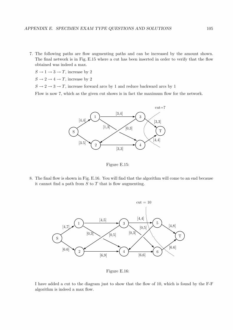
APPENDIX E. SPECIMEN EXAM TYPE QUESTIONS AND SOLUTIONS 105
7. The following paths are flow augmenting paths and can be increased by the amount shown.The final network is in Fig. E.15 where a cut has been inserted in order to verify that the flowobtained was indeed a max.
S → 1 → 3 → T , increase by 2
S → 2 → 4 → T , increase by 2
S → 2 → 3 → T , increase forward arcs by 1 and reduce backward arcs by 1
Flow is now 7, which as the given cut shows is in fact the maximum flow for the network.
1
2
3
4-
-
+ j
S
3
[3,4]
[4,4]
[3,3]
T[1,3]
[4,4]s[3.5]
~
3
[0,3]
[3,3]
cut=7
Figure E.15:
8. The final flow is shown in Fig. E.16. You will find that the algorithm will come to an end becauseit cannot find a path from S to T that is flow augmenting.
1
2
3
4-
-
+ j
S
3
[4,5]
[4,7]
[6,9]
T[0,3]
s[6.6]
5
6
[0,5]
ª -R
-
s
>
[4,4]
[6,6]
[0,5][0,3]
[4,8]
[6.6]
cut = 10
Figure E.16:
I have added a cut to the diagram just to show that the flow of 10, which is found by the F-Falgorithm is indeed a max flow.

APPENDIX E. SPECIMEN EXAM TYPE QUESTIONS AND SOLUTIONS 106
9. Define the following sets:
S6 = {T}, S5 = {10, 11}, S4 = {7, 8, 9}, S3 = {5, 6}, S2 = {1, 2, 3, 4}, S1 = {S}Stage i is defined to have input Si and output Si+1 i = 1 . . . 5.
The decisions at each stage are ’which arc is chosen’ thus the decision sets are:
D5 = {(10, T ), (11, T )}, D4 = {(7, 10), (8, 10), (8, 11), (9, 11)}, D3 = {(5, 8), (6, 7), (6, 8), (6, 9)}D2 = {(1, 5), (2, 5), (2, 6), (3, 5), (3, 6), (4, 6)}, D1 = {(S, 1), (S, 2), (S, 3), (S, 4)}
The state variables at stage i are the elements of the set Si, that is to say the input nodes ateach stage.
Optimization functional:
(i) fi(xi) is the value of the shortest path from stage i with input xi to T . This is defined by:
fi(xi) = minarcs(xi,xi+1)
{fi+1(xi+1) + dist(xi, xi+1)} f6(x6) = 0
(ii) fi(xi) is the value of longest arc on the path from stage i with input xi to T that has thesmallest longest link. This is defined by:
fi(xi) = minarcs(xi,xi+1)
{max[fi+1(xi+1), dist(xi, xi+1)]} f6(x6) = 0
S
2
1
3
4
5
6
8
7
9
10
11
T
µ
1
z
R
s-
-3
*
j
Á
q
j
*
q:
:q
j*
34
2
4
2
2
1
2
4
3
6
6
5
5
2
6
5
3
2
4
(5,T)
[6,T]
[8,10]
[7,10]
[8,11]
[13,8]
[12,8]
[17,5]
[13,6]
[15,5]
[15,6]
[15,2]
[5,T]
(6,T)
(6,11)
(5,10)
(5,10)
(6,8)
(5,7)(5,6)
(5,6)
(6,5)
(5,6)
(5,4)
Figure E.17:
For (i) I have used the notation [fi(xi), xi+1] with square brackets and for (ii) the notation(fi(xi), xi+1) with round brackets. With this type of problem, that it to say a small network,you can put the labels straight on the diagram, as seen in Fig. E.17, starting at nodes 11 and 10and working back to S.
Whenever there is a tie for a choice of arc then randomly select one. Thus the two solutions are:

APPENDIX E. SPECIMEN EXAM TYPE QUESTIONS AND SOLUTIONS 107
(i) S → 2 → 6 → 8 → 10 → T is the shortest path and is equal to 15.
(ii) S → 4 → 6 → 7 → 10 → T is a path that minimizes the longest link; which is 5. Had wemade any other choices that satisfied the optimality criteria then a different path may havebeen obtained but the value 5 would have been the same.
10. Let each stage represent a year in the three year period.
Let xi be the age of the machine at the start of the ith stage (ie the ith year)
The only decision is to Keep or Replace, except at the end when a trade in value is considered.
Let fi(xi) be the net return, including the final trade in value, from state xi to the final tradein.
The following network represents this problem.
3
1
4
1
2
5
1
2
3
µ-
j
s -
z
R
R
Á*µ
R
R
R
R
R
R
State Variables. x1 x2 x3 x4Age of machine
K
K
K
KK
stage 1 stage 2
at start of stage i.
stage 3year 1 year 2 year 3
[19,T]
T
~-3
trade in
[14,T]
[11,T][15, R]
[22, R]
[27, R][35, R]
[35, R]
[25, R]
Figure E.18: The decisions are Replace, Keep. The states are shown inside the nodes; Optimal pathshown in bold.
The optimization functional is given by:
fi(xi) = Max{
fi+1(1) + r(0)− c(0) + s(xi)− 25 Replacefi+1(xi + 1) + r(xi)− c(xi) Keep
}i = 1 . . . 3, f4(x4) = s(x4)
Initially label the nodes x4 as [s(x4),T]
Stage 3
f3(1) = Max{19+15−1+19−25 = 27, Replace; 14+14−1.2 = 26.8, Keep} label = [27,R]
f3(2) = Max{19+15−1+14−25 = 22, Replace; 11+12−1.4 = 21.6, Keep} label = [22,R]
f3(5) = {19 + 15− 1 + 7− 25 = 15} label = [15,R]

APPENDIX E. SPECIMEN EXAM TYPE QUESTIONS AND SOLUTIONS 108
Stage 2
f2(1) = Max{27+15−1+19−25 = 35, Replace; 22+14−1.2 = 34.8, Keep} label = [35,R]
f2(4) = Max{27+15−1+9−25 = 25, Replace; 15+5−2.1 = 17.9, Keep} label = [25,R]
Stage 1
f1(3) = Max{35+15−1+11−25 = 35, Replace; 25+9−1.7 = 32.3, Keep} label = [35,R]
Thus the best strategy is to replace the machine every year, this give a net return over the threeyear period, including the final trade in , of £35,000.
11. Define the stage to be the process of allocating the amount of type i cargo to the ship. Letthe state variable xi be the number of tonnes available just before allocating type i cargo. Thedecision variable, di is the number of units allocated consistent with the optimization criteria.The functional fi(xi) is the largest overall possible return from stages i to completion, for inputxi at stage i.
The network in Fig. E.19 represents the allocation of the loads bearing in mind the weight ofeach type of load and the overall maximum load that can be carried.
6
6
3
0
6
2
3
0
0
µ
1
z
--
~-
3-j
R
stage 1
load type 1
stage 2 stage 3
load type 2 load type 3
State Variables. x1 x2 x3 x4Available space
0
1
2
0
1
0
0
6
2
3
0
at start of stage i.
[90,0]
[30,0]
[45,0]
[0,0]
[0,0]
[90,6]
[0,0]
[45,3]
[90,6]
Figure E.19: The decisions di are shown on each arc of the network.
Label the final node [0,0] and then label backwards with [fi(xi), xi+1] i = 3 . . . 1.
At stage 3:
At this stage there is only one possible label for each x3
x3 = 6 : load with 6 units of type 3 to give return 90 label = [90,0]
x3 = 2 : load with 2 units of type 3 to give return 30 label = [30,0]
x3 = 3 : load with 3 units of type 3 to give return 45 label = [45,0]

APPENDIX E. SPECIMEN EXAM TYPE QUESTIONS AND SOLUTIONS 109
x3 = 0 : load with 0 units of type 3 to give zero return label = [0,0]
At stage 2:
x2 = 6, f2(6) = Max{d2 = 0, 90 + 0 = 90 : d2 = 1, 30 + 50 = 80} = 90 label = [90,6]
x2 = 3, f2(6) = Max{d2 = 0, 45 + 0 = 90} = 45 label = [45,3]
x2 = 0, f2(6) = Max{d2 = 0, 0 + 0 = 0} = 0 label = [0,0]
At stage 1:
x1 = 6, f1(6) = Max{d1 = 0, 90 + 0 = 90 : d1 = 1, 45 + 30 = 75 : d1 = 2, 0 + 60 = 60} = 90label = [90,6]
Thus from the last label the max return is 90 and the loading should be, zero tonnes of type 2,zero tonnes of type 2 and 6 tonnes of type 3. The path in the network is indicated in bold.
Finally, though not specifically asked for, the optimization functional fi is given by the recurrencerelation:
fi(xi) = max(xi,xi+1)
{fi+1(xi+1) + di × ri} i = 1 . . . 3 f4(x4) = 0
12. In Fig. E.20 the feasible region is OAPB. The maximal value of z is at one of the vertices ofthis polygon. The coordinates of P are given by:
2x1 + x2 = 4, x1 + 2x2 = 4 ⇒ x1 = x2 =43
and the coordinates of A and B are (0, 2) and (2, 0) respectively. By direct evaluation or bydrawing a test line for the objective function with some value of z, shown as z = 3 in Fig. E.20,the maximum value of z is at P . Thus the maximum value of z = 3× 4
3 + 2× 43 = 20
3 and isattained at x1 = x2 = 4
3 .
• The second and third constraints are binding. (used to find P above)
• If x1 and x2 are in the feasible region then x1 + x2 ≤ 3, thus for δ ≥ 0, x1 + x2 ≤ 3 + δ.Thus P is still the maximal point and hence ∆z = 0. The ratio ∆z
δ = 0 is the dual orshadow price corresponding to constraint (i). This is always zero if the constraint is notbinding.
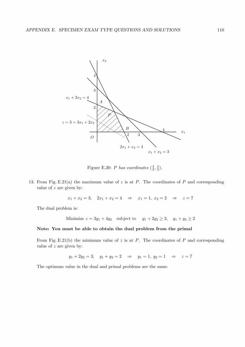
APPENDIX E. SPECIMEN EXAM TYPE QUESTIONS AND SOLUTIONS 110
4
4
3
3
2
2
x1
x2
O
A
P
B
....................................
x1 + x2 = 32x1 + x2 = 4
x1 + 2x2 = 4
z = 3 = 3x1 + 2x2
Figure E.20: P has coordinates (43 , 4
3).
13. From Fig. E.21(a) the maximum value of z is at P . The coordinates of P and correspondingvalue of z are given by:
x1 + x2 = 3, 2x1 + x2 = 4 ⇒ x1 = 1, x2 = 2 ⇒ z = 7
The dual problem is:
Minimize z = 3y1 + 4y2 subject to y1 + 2y2 ≥ 3, y1 + y2 ≥ 2
Note: You must be able to obtain the dual problem from the primal
From Fig. E.21(b) the minimum value of z is at P . The coordinates of P and correspondingvalue of z are given by:
y1 + 2y2 = 3, y1 + y2 = 2 ⇒ y1 = 1, y2 = 1 ⇒ z = 7
The optimum value in the dual and primal problems are the same.

APPENDIX E. SPECIMEN EXAM TYPE QUESTIONS AND SOLUTIONS 111
3
3
4
P
A
2
x1 + x2 = 3
x1
x2
O
............................................
z = 4 = 3x1 + 2x2
B
2x1 + x2 = 4
(a)
y1
y2
y1 + y2 = 2
y1 + 2y2 = 3
B
P
A
3
32
2
2
(b)
......................................................................................................z = 10 = 3y1 + 4y2
Figure E.21: Feasible region shown hashed in each case. (a) P has coordinates (43 , 4
3). Dotted testobjective line with z = 3 (b) P has coordinates (1, 1). Dotted test objective line with z = 10
14.With x1 equal to the number of lectures given for the Maths Dept and x2 the number for the
15
15
A
P
B
x1 + x2 = 15
x1
x2
O
x1 + 1.5x2 = 19
19
12 23
(a)
5
5
A
P
B
y1 + y2 = 5
y1
y2
O
y1 + 1.5y2 = 7
19
4 23
(b)
Figure E.22: Feasible region shown hashed in each case. (a) P has coordinates (43 , 4
3). Dotted testobjective line with z = 3 (b) P has coordinates (1, 1). Dotted test objective line with z = 10
Act Sci Dept the primal problem is:
Maximize z = 5x1 + 7x2 subject to x1 + x2 ≤ 15, x1 + 1.5x2 ≤ 19 x1, x2,≥ 0
In Fig. E.22(a) the maximum value of z is at P (check by evaluating z at A,P and B or bydrawing a test line). Thus the solution is:
x1 + x2 = 15, x1 + 1.5x2 = 19 ⇒ x1 = 7, x2 = 8 ⇒ z = 5× 7 + 7× 8= 91

APPENDIX E. SPECIMEN EXAM TYPE QUESTIONS AND SOLUTIONS 112
Thus in any one week I should lecture 7hours for Maths and 8hours for Act Sci in order to giveme a return of £91.
The dual problem is given by;
Minimize z = 15y1 + 19y2 such that y1 + y2 ≥ 5, y1 + 1.5y2 ≥ 7 y1, y2 ≥ 0
In Fig. E.22(b) the minimum value of z is at P (check by evaluating z at A,P and B or bydrawing a test line). Thus the solution is:
y1 + y2 = 5, y1 + 1.5y2 = 7 ⇒ y1 = 1, y2 = 4 ⇒ z = 15× 1 + 19× 4= 91
Thus we see that the optimal values are the same for both the primal and dual problems.
The interpretation of the dual is important. From the point of view of the employer theywish to cost out the lecturer’s job by paying so much an hour for an actual lecture (denote asy1) and so much for preparation (denote as y2), irrespective of in which department the workis undertaken. That is to say they wish to have a single policy for the whole institution. Sincethe lecturer has agreed to work in a given week a total of 15hrs actual lecture contact and 19hrspreparation the cost to the institution in a given week is z = 15y1 + 19y2; the new objectivefunction for the dual problem, an amount the institution would like to minimize. In order to atleast maintain the levels of payment to the lecturer the rates must be such that the payment forthe work carried out in the Math Dept to deliver 1 lecture must be at least £5. Thus y1 +y2 ≥ 5.Similarly a single lecture in Act Sci department must generate at least £7, thus y1 + 1.5y2 ≥ 7.These are the two dual constraints.
The solution is a little unrealistic in the sense that the rate for giving the lecture is only £1 /hrand for preparation it is £4/hr.
15. Set x1 = 0, this will yield a basic solution since the other two columns, namely( −1
1
)and
(21
)are independent.
Thus solve:
x2
( −11
)+x3
(21
)=
(41
)⇒ x3 = 5/3, x2 = −2/3, x1 = 0 not feasible since not all ≥ 0
Similarly x2 = 0 gives:
x1
(12
)+x3
(21
)=
(41
)⇒ x3 = 7/3, x1 = −2/3, x2 = 0 not feasible since not all ≥ 0
and x3 = 0 gives:
x1
(12
)+x2
( −11
)=
(41
)⇒ x2 = −7/3, x1 = 5/3, x3 = 0 not feasible since not all ≥ 0
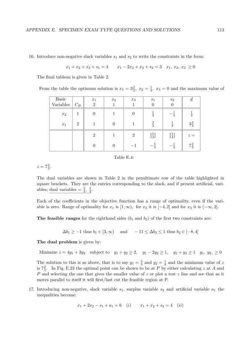
APPENDIX E. SPECIMEN EXAM TYPE QUESTIONS AND SOLUTIONS 113
16. Introduce non-negative slack variables s1 and s2 to write the constraints in the form:
x1 + x2 + x3 + s1 = 4 x1 − 2x2 + x3 + s2 = 3 x1, x2, x3 ≥ 0
The final tableau is given in Table 2.
From the table the optimum solution is x1 = 323 , x2 = 1
3 , x3 = 0 and the maximum value of
Basic x1 x2 x3 s1 s2 dVariables CB 2 1 1 0 0
x2 1 0 1 0 13 −1
313
x1 2 1 0 1 23
13 32
3
2 1 2 [53 ] [1
3 ] z =
0 0 −1 −53 −1
3 723
Table E.4:
z = 723 .
The dual variables are shown in Table 2 in the penultimate row of the table highlighted insquare brackets. They are the entries corresponding to the slack, and if present artificial, vari-ables; dual variables = 5
3 , 13 .
Each of the coefficients in the objective function has a range of optimality, even if the vari-able is zero. Range of optimality for x1 is [1,∞), for x2 it is [−4, 2] and for x3 it is (−∞, 2].
The feasible ranges for the righthand sides (b1 and b2) of the first two constraints are:
∆b1 ≥ −1 thus b1 ∈ [3,∞) and − 11 ≤ ∆b2 ≤ 1 thus b2 ∈ [−8, 4]
The dual problem is given by:
Minimize z = 4y1 + 3y2 subject to y1 + y2 ≥ 2, y1 − 2y2 ≥ 1, y1 + y2 ≥ 1 y1, y2, ≥ 0
The solution to this is as above, that is to say y1 = 53 and y2 = 1
3 and the minimum value of z
is 723 . In Fig. E.23 the optimal point can be shown to be at P by either calculating z at A and
P and selecting the one that gives the smaller value of z or plot a test z line and see that as itmoves parallel to itself it will first/last cut the feasible region at P.
17. Introducing non-negative, slack variable s1, surplus variable s2 and artificial variable a1 theinequalities become:
x1 + 2x2 − s1 + a1 = 6 (i) x1 + x2 + s2 = 4 (ii)

APPENDIX E. SPECIMEN EXAM TYPE QUESTIONS AND SOLUTIONS 114
2
A
2y1 + y2 = 1
P
1
y1 + y2 = 2
y1
y2
O 1
y1 − 2y2 = 1
...............................................................................z = 6 = 4y1 + 3y2
Figure E.23: Feasible region shown hashed. Optimal point at P which has coordinates (53 , 1
3) givingz = 71
3 . Dotted test objective line shown with z = 6
I have reordered the equations so that the slack and artificial variables appear last and thus thebody of the first Simplex tableau will be of the form (D I).
The objective function is z = 2x1 + x2 + 0s1 + 0s2 −Ma1, the −M ensures that the artificialvariable is forced to zero when maximizing.
The optimal tableau is:
Basic x1 x2 s1 a1 s2 dVariables CB 2 1 0 −M 0
x2 1 0 1 -1 1 −1 2
x1 2 1 0 1 −1 2 2
2 1 1 [−1] [3] z =
0 0 −1 −M + 1 −3 6
Table E.5:
The optimal solution is that the minimum value of z is 6 with x1 = x2 = 2.
The dual variables are given in the penultimate row in the columns corresponding to theartificial and slack variables, not to the surplus variable. Corresponding to equation (i) thedual variable is −1 and to equation (ii) it is +3.
Range of optimality for the x1 coefficient is [0.5,∞) and for x2 it is (−∞, 2].
The feasible range for the righthand side of (i) is [4, 8] and for (ii) it is [3, 6].

APPENDIX E. SPECIMEN EXAM TYPE QUESTIONS AND SOLUTIONS 115
18. The five inequalities and objective function, with the xi non-negative, are:
2x1 + x2 + x3 ≤ 35, 3x1 + x2 + 4x3 ≤ 40 x1 + x2 + x3 ≤ 30
2x1 + 3x2 + x3 ≤ 60, 3x1 + x2 ≤ 20 and z = 1250x1 + 1500x2 + 750x3
From the given data the optimum production is: Max z = £31, 429 attained by producing 0.714tonnes of Milk Chocolate, 17.857 tonnes of Plain chocolate and 5 tonnes of Toffee.
Shadow (dual) price is max for constraint (d) thus a small increase in this resource will yieldthe most profit. The maximum increase in this department consistent with this basic solutionis 5units to 65.
If xi = 0 in the optimal solution then the reduced cost corresponding to xi is the amount thecoefficient of xi in the objective function needs to be changed so that there exists an optimalsolution with xi 6= 0. In this problem all variables are non-zero thus no increase is needed, hencethe reduced costs are all zero.
The dual problem, with the yi non-negative, is to minimize:
z = 35y1 + 40y2 + 30y3 + 60y4 + 20y5
subject to:
2y1 + 3y2 + y3 + 2y4 + 3y5 ≥ 1250, y1 + y2 + y3 + 3y4 + y5 ≥ 1500, y1 + 4y2 + y3 + y4 ≥ 750
The shadow variables (prices) are the solutions to the dual problem, thus:
y1 = 0, y2 = 71.43, y3 = 0, y4 = 464.29, y5 = 35.71
The minimum value of z is of course the same as before, namely z = 31, 429
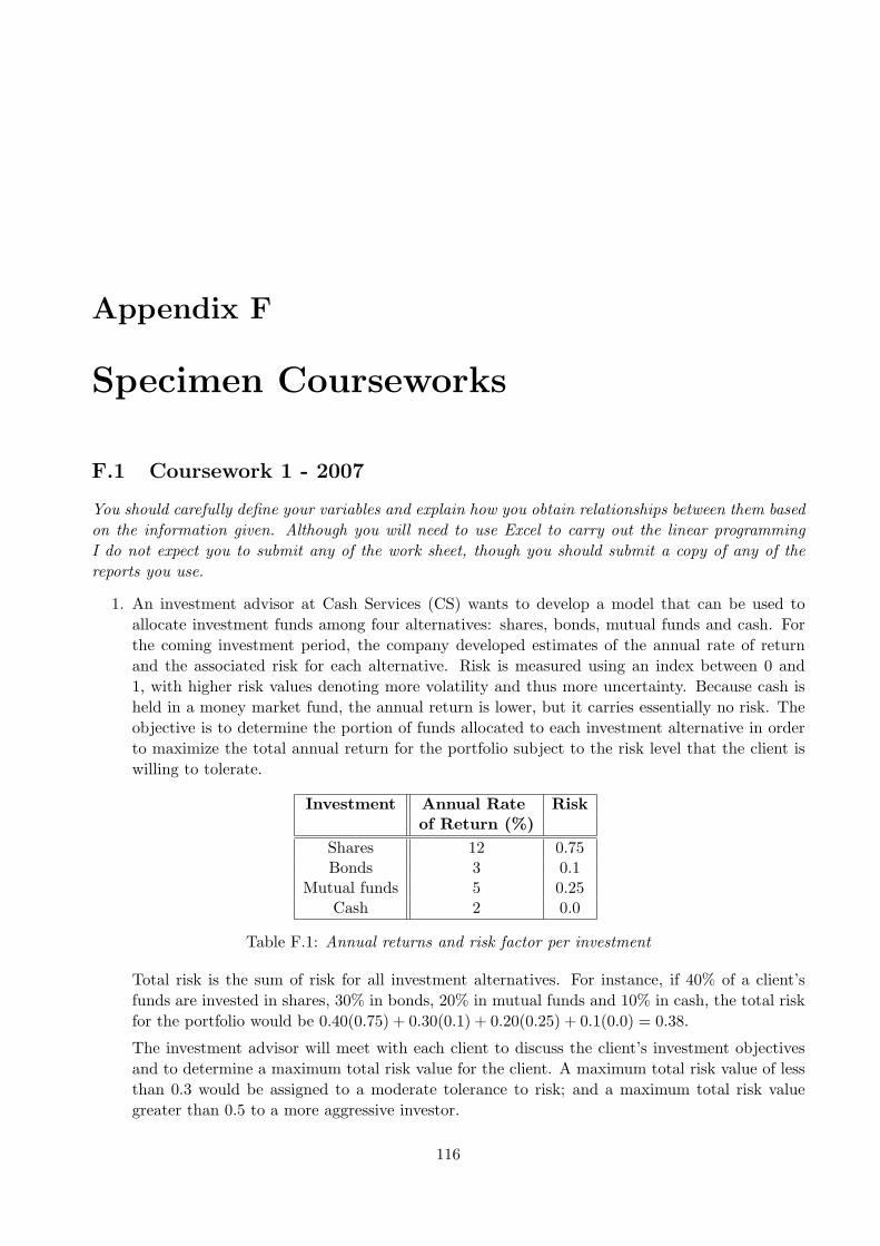
Appendix F
Specimen Courseworks
F.1 Coursework 1 - 2007
You should carefully define your variables and explain how you obtain relationships between them basedon the information given. Although you will need to use Excel to carry out the linear programmingI do not expect you to submit any of the work sheet, though you should submit a copy of any of thereports you use.
1. An investment advisor at Cash Services (CS) wants to develop a model that can be used toallocate investment funds among four alternatives: shares, bonds, mutual funds and cash. Forthe coming investment period, the company developed estimates of the annual rate of returnand the associated risk for each alternative. Risk is measured using an index between 0 and1, with higher risk values denoting more volatility and thus more uncertainty. Because cash isheld in a money market fund, the annual return is lower, but it carries essentially no risk. Theobjective is to determine the portion of funds allocated to each investment alternative in orderto maximize the total annual return for the portfolio subject to the risk level that the client iswilling to tolerate.
Investment Annual Rate Riskof Return (%)
Shares 12 0.75Bonds 3 0.1
Mutual funds 5 0.25Cash 2 0.0
Table F.1: Annual returns and risk factor per investment
Total risk is the sum of risk for all investment alternatives. For instance, if 40% of a client’sfunds are invested in shares, 30% in bonds, 20% in mutual funds and 10% in cash, the total riskfor the portfolio would be 0.40(0.75) + 0.30(0.1) + 0.20(0.25) + 0.1(0.0) = 0.38.
The investment advisor will meet with each client to discuss the client’s investment objectivesand to determine a maximum total risk value for the client. A maximum total risk value of lessthan 0.3 would be assigned to a moderate tolerance to risk; and a maximum total risk valuegreater than 0.5 to a more aggressive investor.
116

APPENDIX F. SPECIMEN COURSEWORKS 117
CS specifies additional guidelines that must be applied to all clients. Namely:
• No more than 65% of the total investment may be in shares
• The amount invested in mutual funds must be at least as much as invested in bonds.
• The amount of cash must be at least 15%, but no more than 40% of the total investmentfunds.
(a) Suppose the maximum risk value for a particular client is 0.3. What is the optimal allocationof investment funds among shares, bonds, mutual funds and cash? What is the annual rateof return and the total risk for the optimal portfolio?
(b) Suppose the maximum risk value of a more conservative client is 0.15. What is the optimalallocation of investment funds for this client? What is the annual rate of return and thetotal risk for the optimal portfolio.
(c) Another more aggressive client has a maximum risk value of 0.8. What is the optimalallocation of investment funds for this client? What is the annual rate of return and thetotal risk for the optimal portfolio.
(d) Refer to the solution for the more aggressive client in part (c). Would this client beinterested in having the investment advisor increase the maximum percentage allowed inshares or decrease the requirement that the amount of cash must be at least 15% of thefunds invested?
2. Soft Things is a company making objects out of polystyrene. Next weeks schedule calls for theproduction of 80,000 small sandwich containers, 80,000 large sandwich containers and 65,000meal containers. With the exception of the meal container, all these products can be processedon any one of three machines available. However the amount of waste produced varies fromitem to item and machine to machine. The amounts of waste are given in the following table;measured in milligrams per item.
Machine Small LargeType Sandwich Sandwich MealM1 20 15 −M2 24 28 18M3 32 35 36
Table F.2: The amount of waste per item measured in milligrams
The time for each type of machine to produce each item also varies with machine and item; thefollowing table gives the number of items produced on each machine per minute:
The availability of each machine in the following week is 35 hours for machine M1, 35 hours formachine M2 and 40 hours for machine M3.
(a) Costs reprocessing the waste have risen, thus Soft Things would like to minimize the totalamount of waste produce. Formulate the linear programming model to determine the bestproduction schedule.
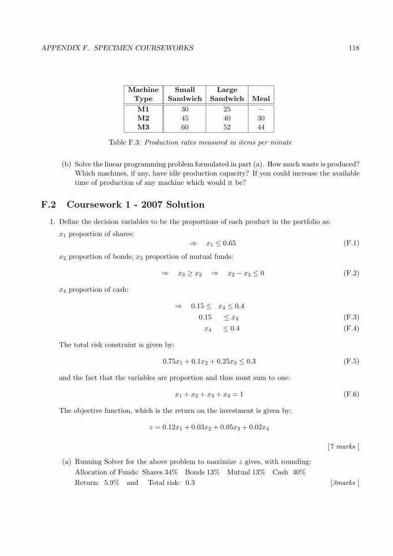
APPENDIX F. SPECIMEN COURSEWORKS 118
Machine Small LargeType Sandwich Sandwich MealM1 30 25 −M2 45 40 30M3 60 52 44
Table F.3: Production rates measured in items per minute
(b) Solve the linear programming problem formulated in part (a). How much waste is produced?Which machines, if any, have idle production capacity? If you could increase the availabletime of production of any machine which would it be?
F.2 Coursework 1 - 2007 Solution
1. Define the decision variables to be the proportions of each product in the portfolio as:
x1 proportion of shares:⇒ x1 ≤ 0.65 (F.1)
x2 proportion of bonds; x3 proportion of mutual funds:
⇒ x3 ≥ x2 ⇒ x2 − x3 ≤ 0 (F.2)
x4 proportion of cash:
⇒ 0.15 ≤ x4 ≤ 0.4
0.15 ≤ x4 (F.3)
x4 ≤ 0.4 (F.4)
The total risk constraint is given by:
0.75x1 + 0.1x2 + 0.25x3 ≤ 0.3 (F.5)
and the fact that the variables are proportion and thus must sum to one:
x1 + x2 + x3 + x3 = 1 (F.6)
The objective function, which is the return on the investment is given by;
z = 0.12x1 + 0.03x2 + 0.05x3 + 0.02x4
[7 marks ]
(a) Running Solver for the above problem to maximize z gives, with rounding:Allocation of Funds: Shares 34% Bonds 13% Mutual 13% Cash 40%Return: 5.9% and Total risk: 0.3 [3marks ]

APPENDIX F. SPECIMEN COURSEWORKS 119
(b) Changing the risk constraint in Eq(F.5) from 0.3 to 0.15 gives:Allocation of Funds: Shares 8% Bonds 26% Mutual 26% Cash 40%Return: 3.8% and Total risk: 0.15 [3 marks ]
(c) Again changing the Risk in Eq(F.5), now from 0.3 to 0.8 gives:Allocation of Funds: Shares 65% Bonds 0% Mutual 20% Cash 15%Return: 9.1% and Total risk: 0.5375 [3 marks ]
(d) For the data in (c) Fig. F.1 shows the spreadsheet and the Sensitivity and Answer Reportfrom Excel.With reference to the constraints section note that the shadow price for constraint (1),which corresponds to shares, is 0.07 and the shadow price for constraint (3), correspondingto the lower limit on cash, is -0.03.Thus an increase in the level of allowed shares purchased gives an increase of 0.07 in thereturn. In terms of the units an increase of 0.1 in the allowed proportion of shares is anincrease of 10% points which corresponds to an increase in the return of 0.7% points.Since the amount of cash is decreased then an increase of 0.03 is reflected in the return.Again in the units of the question if the lower limit is reduced by 0.1, that is to say 10%points, then the return is increased by 0.3% points.Thus the client may well be more interested in increasing the maximum percentage of sharesin the portfolio rather than decreasing the lower restriction on the amount of cash. [5marks ]
[4 marks ]
[Total 25 marks ]
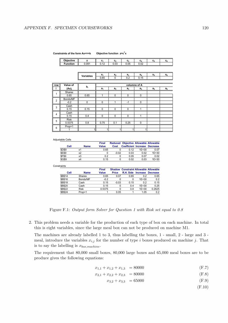
APPENDIX F. SPECIMEN COURSEWORKS 120
Constraints of the form Ax<=>b Objective function z=cTx
Objective z c1 c2 c3 c4 c5 c6
Function 0.091 0.12 0.03 0.05 0.02
x1 x2 x3 x4 x5 x6
0.65 0 0.2 0.15
row Value of
i (Ax)i a1 a2 a3 a4 a5 a6
Shares0.65 0.65 1 0 0 0
Bonds/MF-0.2 0 0 1 -1 0
Cash0.15 0.15 0 0 0 1
Cash0.15 0.4 0 0 0 1
Risk0.5375 0.8 0.75 0.1 0.25 0
Prop=11 1 1 1 1 1
Adjustable Cells
Final Reduced Objective Allowable Allowable
Cell Name Value Cost Coefficient Increase Decrease
$D$9 x1 0.65 0 0.12 1E+30 0.07
$E$9 x2 0 -0.02 0.03 0.02 1E+30
$F$9 x3 0.2 0 0.05 0.07 0.02$G$9 x4 0.15 0 0.02 0.03 1E+30
Constraints
Final Shadow Constraint Allowable Allowable
Cell Name Value Price R.H. Side Increase Decrease
$B$14 Shares 0.65 0.07 0.65 0.2 0.65
$B$16 Bonds/MF -0.2 0 0 1E+30 0.2
$B$18 Cash 0.15 -0.03 0.15 0.2 0.15
$B$20 Cash 0.15 0 0.4 1E+30 0.25
$B$22 Risk 0.5375 0 0.8 1E+30 0.2625$B$24 Prop=1 1 0.05 1 1.05 0.2
6
2
3
4
5
columns of Abi
Variables
1
Figure F.1: Output form Solver for Question 1 with Risk set equal to 0.8
2. This problem needs a variable for the production of each type of box on each machine. In totalthis is eight variables, since the large meal box can not be produced on machine M1.
The machines are already labelled 1 to 3, thus labelling the boxes, 1 - small, 2 - large and 3 -meal, introduce the variables xi,j for the number of type i boxes produced on machine j. Thatis to say the labelling is xbox,machine.
The requirement that 80,000 small boxes, 80,000 large boxes and 65,000 meal boxes are to beproduce gives the following equations:
x1,1 + x1,2 + x1,3 = 80000 (F.7)
x2,1 + x2,2 + x2,3 = 80000 (F.8)
x3,2 + x3,3 = 65000 (F.9)
(F.10)
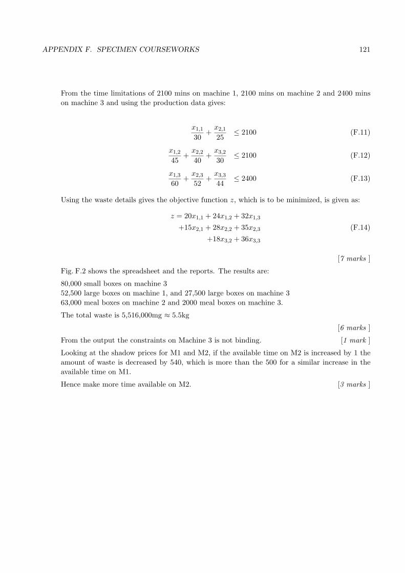
APPENDIX F. SPECIMEN COURSEWORKS 121
From the time limitations of 2100 mins on machine 1, 2100 mins on machine 2 and 2400 minson machine 3 and using the production data gives:
x1,1
30+
x2,1
25≤ 2100 (F.11)
x1,2
45+
x2,2
40+
x3,2
30≤ 2100 (F.12)
x1,3
60+
x2,3
52+
x3,3
44≤ 2400 (F.13)
Using the waste details gives the objective function z, which is to be minimized, is given as:
z = 20x1,1 + 24x1,2 + 32x1,3
+15x2,1 + 28x2,2 + 35x2,3
+18x3,2 + 36x3,3
(F.14)
[7 marks ]
Fig. F.2 shows the spreadsheet and the reports. The results are:
80,000 small boxes on machine 352,500 large boxes on machine 1, and 27,500 large boxes on machine 363,000 meal boxes on machine 2 and 2000 meal boxes on machine 3.
The total waste is 5,516,000mg ≈ 5.5kg
[6 marks ]
From the output the constraints on Machine 3 is not binding. [1 mark ]
Looking at the shadow prices for M1 and M2, if the available time on M2 is increased by 1 theamount of waste is decreased by 540, which is more than the 500 for a similar increase in theavailable time on M1.
Hence make more time available on M2. [3 marks ]

APPENDIX F. SPECIMEN COURSEWORKS 122
constraints Availability Use X11 X12 X13 X21 X22 X23 X32 X33
M1 2100 2100 0.0333333 0 0 0.04 0 0 0 0
M2 2100 2100 0 0.0222222 0 0 0.03 0 0.03 0
M3 2400 1907.634033 0 0 0.0166667 0 0 0.02 0 0.02
Demand 1 80000 80000 1 1 1 0 0 0 0 0
Demand 1 80000 80000 0 0 0 1 1 1 0 0
Demand 3 65000 65000 0 0 0 0 0 0 1 1
x11 x12 x13 x21 x22 x23 x32 x33
0.000 0.000 80000.000 52500.000 0 27500 63000 2000
z c1 c2 c3 c4 c5 c6 c8 c9
5516000 20 24 32 15 28 35 18 36
Final Reduced Obj Max Max
Cell Name Value Cost Coft Increase Decrease
$A$12 x11 0.000 4.667 20 1E+30 4.666667
$B$12 x12 0.000 4.000 24 1E+30 4
$C$12 x13 80000.000 0.000 32 4 1E+30
$D$12 x21 52500.000 0.000 15 5.6 1E+30
$E$12 x22 0 6.5 28 1E+30 6.5
$F$12 x23 27500 0 35 6.5 5.6
$G$12 x32 63000 0 18 6 1E+30$H$12 x33 2000.000005 0 36 1E+30 6
Final Shadow Max Max
Cell Name Value Price R.H. S Increase Decrease
$C$3 M1 Use 2100 -500 2100 1100 1024.121
$C$4 M2 Use 2100 -540 2100 66.666667 722.1368
$C$5 M3 Use 1907.634033 0 2400 1E+30 492.366
$C$6 Demand 1 80000 32 80000 29541.958 80000
$C$7 Demand 1 80000 35 80000 25603.03 27500$C$8 Demand 3 65000 36 65000 21664.103 2000
Cell Name Orig Value Fin Value
$A$16 z 6862363.636 5516000
Cell Name Orig Value Fin Value
$A$12 x11 20136.364 0.000
$B$12 x12 4500.000 0.000
$C$12 x13 55363.636 80000.000
$D$12 x21 0.000 52500.000
$E$12 x22 80000 0
$F$12 x23 0 27500
$G$12 x32 0 63000$H$12 x33 65000 2000
Cell Name Cell Value Formula Status Slack
$C$3 M1 Use 2100 $C$3<=$B$3 Binding 0
$C$4 M2 Use 2100 $C$4<=$B$4 Binding 0
$C$5 M3 Use 1907.634033 $C$5<=$B$5Not Binding 492.36597
$C$6 Demand 1 80000 $C$6=$B$6 Not Binding 0
$C$7 Demand 1 80000 $C$7=$B$7 Not Binding 4.657E-06$C$8 Demand 3 65000 $C$8=$B$8 Not Binding 0
Objective Function
Variables
Figure F.2: Output form Solver for Question 2
[3 marks ]
[Total 20 marks ]

APPENDIX F. SPECIMEN COURSEWORKS 123
F.3 Coursework 2 - 2007
1. Obtain all feasible basic solutions for the equations
−x1 + x2 + x3 + x4 = 1
x1 − x2 + x3 + x4 = 1
x1 + x2 − x3 + x4 = 1
The following two questions must be done using the Simplex Tableau method with the relevanttableaus at each stage being submitted.
2. Using the Simplex Method maximize z = 3x1 + x2 + 2x3 subject to
x1 + x2 + 2x3 ≤ 4 (i) 2x1 + x2 − x3 ≤ 2 (ii)
From your final tableau:
(a) Find the dual prices of (i) and (ii)
(b) Find the feasible range for the righthand sides of (i).
(c) Find the optimal ranges for the coefficient of x1 in z.
3. Using the Simplex Method find the maximum value of z = x1 + 3x2 subject to
x1 + x2 ≥ 3 (i) x1 + 2x2 ≤ 4 (ii)
As in question 2 find the dual prices, feasible range for constraint (i) and range of optimality forthe x1 objective function coefficient.
F.4 Coursework 2 - 2007 Solution
1. To form a basic solution select in turn 3 independent columns and solve with the fourth variableequal to zero. In this example it is possible to do this in exactly 4 ways. The number of waysmay be less than this if one selection of columns is not independent - this can happen, but nothere.
Select the first three columns and row reduce to make the first three columns become the identity.(If this had turned out not to be possible then the three columns would not have been independentand thus would not have yielded a basic solution. Remedy - try a different combination of threecolumns.)
−1 1 1 1 1
1 −1 1 1 11 1 −1 1 1
→
1 0 0 1 10 1 0 1 10 0 1 1 1
⇒ x4 = 0, and x1 = x2 = x3 = 1

APPENDIX F. SPECIMEN COURSEWORKS 124
Next select columns 2,3 and 4. Thus continue to row reduce to make col4 into the old column 1to give:
1 0 0 1 1
−1 1 0 0 0−1 0 1 0 0
⇒ x1 = 0, and x2 = x3 = 0, x4 = 1
Next select columns 1,2 and 4. Continue to row reduce to make col1 into the old column 3 togive:
0 0 1 1 10 1 −1 0 01 0 −1 0 0
⇒ x3 = 0, and x1 = x2 = 0, x4 = 1
Finally select columns 1,3 and 4. Continue to row reduce to make col 3 into the old column 2to give:
0 1 0 1 10 −1 1 0 01 −1 0 0 0
⇒ x2 = 0, and x1 = x3 = 0, x4 = 1
In each case the solution underlined is the variable that is set equal to zero, the non-basicvariable.
With regard to Linear Programming all solutions are feasible since greater or equal to zero,however with the exception of the first they are all degenerate since in each case at least one ofthe basic variables is zero.
2. Write asx1 + x2 + 2x3 + s1 = 4 2x1 + x2 − x3 + s2 = 2
with slack variables s1, s2 ≥ 0.
The objective function is now z = 3x1 + x2 + 2x3 + 0s1 + 0s2
To form the simplex tableau always order your variables with the slack and artificial variablelast. This then gives the standard form (D I) in the body of the table. Since this is a maxi-
x1 x2 x3 s1 s2 d da
Basic Var cj 3 1 2 0 0s1 0 1 1 2 1 0 4 4s2 0 2 1 -1 0 1 2 1zj 0 0 0 0 0 z =∆z 3 1 2 0 0 0
Table F.4:
mization problem keep row reducing etc until the final row is non-positive. In the final row 3 isthe largest value so bring in x1 into the basic set. Form the ratio of the d column with column1 and place in the last column. Since 1 is the smallest non-negative value in the final columntake s2 out of the basic set.
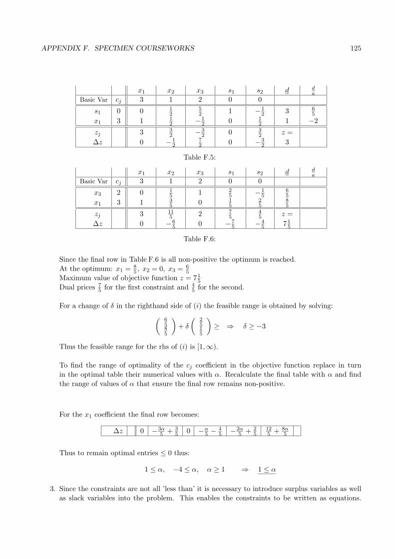
APPENDIX F. SPECIMEN COURSEWORKS 125
x1 x2 x3 s1 s2 d da
Basic Var cj 3 1 2 0 0
s1 0 0 12
52 1 −1
2 3 65
x1 3 1 12 −1
2 0 12 1 −2
zj 3 32 −3
2 0 32 z =
∆z 0 −12
72 0 −3
2 3
Table F.5:
x1 x2 x3 s1 s2 d da
Basic Var cj 3 1 2 0 0
x3 2 0 15 1 2
5 −15
65
x1 3 1 35 0 1
525
85
zj 3 115 2 7
545 z =
∆z 0 −65 0 −7
5 −45 71
5
Table F.6:
Since the final row in Table F.6 is all non-positive the optimum is reached.At the optimum: x1 = 8
5 , x2 = 0, x3 = 65
Maximum value of objective function z = 715
Dual prices 75 for the first constraint and 4
5 for the second.
For a change of δ in the righthand side of (i) the feasible range is obtained by solving:(
6585
)+ δ
(2515
)≥ ⇒ δ ≥ −3
Thus the feasible range for the rhs of (i) is [1,∞).
To find the range of optimality of the cj coefficient in the objective function replace in turnin the optimal table their numerical values with α. Recalculate the final table with α and findthe range of values of α that ensure the final row remains non-positive.
For the x1 coefficient the final row becomes:
∆z 0 −3α5 + 3
5 0 −α5 − 4
5 −2α5 + 2
5125 + 8α
5
Thus to remain optimal entries ≤ 0 thus:
1 ≤ α, −4 ≤ α, α ≥ 1 ⇒ 1 ≤ α
3. Since the constraints are not all ’less than’ it is necessary to introduce surplus variables as wellas slack variables into the problem. This enables the constraints to be written as equations.

APPENDIX F. SPECIMEN COURSEWORKS 126
Additionally since we are to solve using the Simplex method, which starts at the origin, it willbe necessary to introduce an artificial variable a1 to help provide an initial feasible solution.
The final solution should not contain the artificial variable (ie it should be zero), in order toforce this variable to zero an extra term is introduced into the objective function. Since this isa maximization problem we introduce −Ma1 into z, where M is arbitrarily large and positive.
Thus the problem becomes:
x1 + 2x2 + s2 = 4, x1 + x2 − s1 + a1 = 3, z = x1 + 3x2 −Ma1
Where s2, s1, a1 are all ≥ 0. Note s2 is the slack variable, s1 the surplus variable and a1 theartificial variable.
When forming the tableau order the variables so that the slack and artificial variables are last,this gives a standard display of the form (D I). As M is large and positive, 3 + M is the maxi-
x1 x2 s1 s2 a1 d da
Basic Var cj 1 3 0 0 −M
s2 0 1 2 0 1 0 4 2a1 −M 1 1 −1 0 1 3 3
zj −M −M M 0 −M z =∆z 1 + M 3 + M −M 0 0 −3M
Table F.7:
mum value in the final row, thus bring x2 into the basic set. Form the ratio of the d with the x2
column and select the smallest non-negative value to take out of the basic set.(these value are inthe final column) In this case s2. Since M is positive and large, −1
2 + M is the largest positive
x1 x2 s1 s2 a1 d da
Basic Var cj 1 3 0 0 −M
x2 3 12 1 0 1
2 0 2 4a1 −M 1
2 0 −1 −12 1 1 2
zj32 − M
2 3 M 32 + M
2 −M z =∆z −1
2 + M2 0 −M −3
2 − M2 0 6−M
Table F.8:
value in the final row, thus bring x1 into the basic set.
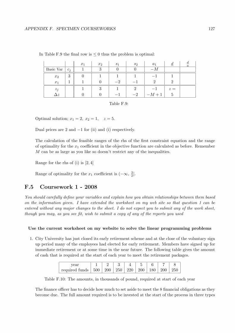
APPENDIX F. SPECIMEN COURSEWORKS 127
In Table F.9 the final row is ≤ 0 thus the problem is optimal:
x1 x2 s1 s2 a1 d da
Basic Var cj 1 3 0 0 −M
x2 3 0 1 1 1 −1 1x1 1 1 0 −2 −1 2 2
zj 1 3 1 2 −1 z =∆z 0 0 −1 −2 −M + 1 5
Table F.9:
Optimal solution; x1 = 2, x2 = 1, z = 5.
Dual prices are 2 and −1 for (ii) and (i) respectively.
The calculation of the feasible ranges of the rhs of the first constraint equation and the rangeof optimality for the x1 coefficient in the objective function are calculated as before. RememberM can be as large as you like so doesn’t restrict any of the inequalities.
Range for the rhs of (i) is [2, 4]
Range of optimality for the x1 coefficient is (−∞, 32 ].
F.5 Coursework 1 - 2008
You should carefully define your variables and explain how you obtain relationships between them basedon the information given. I have extended the worksheet on my web site so that question 1 can beentered without any major changes to the sheet. I do not expect you to submit any of the work sheet,though you may, as you see fit, wish to submit a copy of any of the reports you used
Use the current worksheet on my website to solve the linear programming problems
1. City University has just closed its early retirement scheme and at the close of the voluntary signup period many of the employees had elected for early retirement. Members have signed up forimmediate retirement or at some time in the near future. The following table gives the amountof cash that is required at the start of each year to meet the retirement packages.
year 1 2 3 4 5 6 7 8required funds 500 200 250 220 200 180 200 250
Table F.10: The amounts, in thousands of pound, required at start of each year
The finance officer has to decide how much to set aside to meet the 8 financial obligations as theybecome due. The full amount required is to be invested at the start of the process in three types
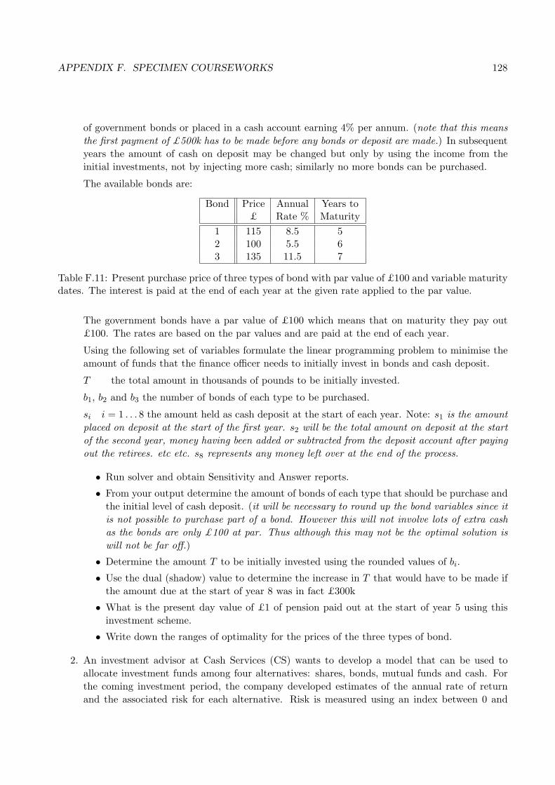
APPENDIX F. SPECIMEN COURSEWORKS 128
of government bonds or placed in a cash account earning 4% per annum. (note that this meansthe first payment of £500k has to be made before any bonds or deposit are made.) In subsequentyears the amount of cash on deposit may be changed but only by using the income from theinitial investments, not by injecting more cash; similarly no more bonds can be purchased.
The available bonds are:
Bond Price Annual Years to£ Rate % Maturity
1 115 8.5 52 100 5.5 63 135 11.5 7
Table F.11: Present purchase price of three types of bond with par value of £100 and variable maturitydates. The interest is paid at the end of each year at the given rate applied to the par value.
The government bonds have a par value of £100 which means that on maturity they pay out£100. The rates are based on the par values and are paid at the end of each year.
Using the following set of variables formulate the linear programming problem to minimise theamount of funds that the finance officer needs to initially invest in bonds and cash deposit.
T the total amount in thousands of pounds to be initially invested.
b1, b2 and b3 the number of bonds of each type to be purchased.
si i = 1 . . . 8 the amount held as cash deposit at the start of each year. Note: s1 is the amountplaced on deposit at the start of the first year. s2 will be the total amount on deposit at the startof the second year, money having been added or subtracted from the deposit account after payingout the retirees. etc etc. s8 represents any money left over at the end of the process.
• Run solver and obtain Sensitivity and Answer reports.
• From your output determine the amount of bonds of each type that should be purchase andthe initial level of cash deposit. (it will be necessary to round up the bond variables since itis not possible to purchase part of a bond. However this will not involve lots of extra cashas the bonds are only £100 at par. Thus although this may not be the optimal solution iswill not be far off.)
• Determine the amount T to be initially invested using the rounded values of bi.
• Use the dual (shadow) value to determine the increase in T that would have to be made ifthe amount due at the start of year 8 was in fact £300k
• What is the present day value of £1 of pension paid out at the start of year 5 using thisinvestment scheme.
• Write down the ranges of optimality for the prices of the three types of bond.
2. An investment advisor at Cash Services (CS) wants to develop a model that can be used toallocate investment funds among four alternatives: shares, bonds, mutual funds and cash. Forthe coming investment period, the company developed estimates of the annual rate of returnand the associated risk for each alternative. Risk is measured using an index between 0 and

APPENDIX F. SPECIMEN COURSEWORKS 129
1, with higher risk values denoting more volatility and thus more uncertainty. Because cash isheld in a money market fund, the annual return is lower, but it carries essentially no risk. Theobjective is to determine the portion of funds allocated to each investment alternative in orderto maximize the total annual return for the portfolio subject to the risk level that the client iswilling to tolerate.
Investment Annual Rate Riskof Return (%)
Shares 7 0.8Bonds 5 0.2
Mutual funds 4 0.3Cash 3 0.0
Table F.12: Annual returns and risk factor per investment
Total risk is the sum of risk for all investment alternatives. For instance, if 40% of a client’sfunds are invested in shares, 30% in bonds, 20% in mutual funds and 10% in cash, the total riskfor the portfolio would be 0.40(0.8) + 0.30(0.2) + 0.20(0.3) + 0.1(0.0) = 0.44.
The investment advisor will meet with each client to discuss the client’s investment objectivesand to determine a maximum total risk value for the client. A maximum total risk value of lessthan 0.3 would be assigned to a moderate tolerance to risk; and a maximum total risk valuegreater than 0.5 to a more aggressive investor.
CS specifies additional guidelines that must be applied to all clients. Namely:
• No more than 60% of the total investment may be in shares
• The amount invested in mutual funds must be at least as much as invested in bonds.
• The amount of cash must be at least 15%, but no more than 30% of the total investmentfunds.
(a) Suppose the maximum risk value for a particular client is 0.4. What is the optimal allocationof investment funds among shares, bonds, mutual funds and cash? What is the annual rateof return and the total risk for the optimal portfolio?
(b) Suppose the maximum risk value of a more conservative client is 0.18. What is the optimalallocation of investment funds for this client? What is the annual rate of return and thetotal risk for the optimal portfolio.
(c) Another more aggressive client has a maximum risk value of 0.7. What is the optimalallocation of investment funds for this client? What is the annual rate of return and thetotal risk for the optimal portfolio.
(d) Refer to the solution for the more aggressive client in part (c). By looking at the dual valueswould this client be interested in having the investment advisor increase the maximumpercentage allowed in shares or decrease the requirement that the amount of cash must beat least 15% of the funds invested?

APPENDIX F. SPECIMEN COURSEWORKS 130
F.6 Coursework 1 - 2008 Solutions
1. The linear programming problem is:
Minimize T given by:
T = 0.115b1 + 0.100b2 + 0.135b3 + 500 + s1 [2 marks]
The funds available to pay out the retirees at the start of all but the first year are generatedfrom the cash investment plus the return on the bonds, any surplus being put back into the cashinvestment. Thus:
200 = 0.0085b1 + 0.0055b2 + 0.0115b3 + 1.04s1 − s2
250 = 0.0085b1 + 0.0055b2 + 0.0115b3 + 1.04s2 − s3
220 = 0.0085b1 + 0.0055b2 + 0.0115b3 + 1.04s3 − s4
200 = 0.0085b1 + 0.0055b2 + 0.0115b3 + 1.04s4 − s5
180 = 0.1085b1 + 0.0055b2 + 0.0115b3 + 1.04s5 − s6
200 = 0.1055b2 + 0.0115b3 + 1.04s6 − s7
250 = 0.1115b3 + 1.04s7 − s8
Note that after 5 years, at the start of year 6 when the finance officer has to find 180 thebonds of type 1 mature, hence the 0.1085b1 term; after that date they obviously give no moreincome.Similary the other two bonds mature over the next two years. [4 marks ]
Target Cell (Min)
Cell Name Final Value
$C$5 Function z 1743.802639
Adjustable Cells
Final Reduced Objective Allowable Allowable
Cell Name Value Cost Coefficient Increase Decrease
$D$9 b1 1337.63 0.00 0.115 0.0050332 0.002944538
$E$9 b2 1651.33 0.00 0.1 0.00290226 0.000818616
$F$9 b3 2242.15 0.00 0.135 0.00092113 0.076078214
$G$9 S1 622.15 0.00 1 0.27781572 0.041931736
$H$9 S2 493.27 0.00 0 0.36339059 0.043264889
$I$9 S3 309.24 0.00 0 0.53467197 0.044744369
$J$9 S4 147.85 0.00 0 1.04877964 0.046394321
$K$9 S5 0.00 0.05 0 1E+30 0.048244502
$L$9 S6 0.00 0.03 0 1E+30 0.028610001
$M$9 S7 0.00 0.01 0 1E+30 0.008591699
$N$9 S8 0.00 0.68 0 1E+30 0.682315823
Constraints
Final Shadow Constraint Allowable Allowable
Cell Name Value Price R.H. Side Increase Decrease
$B$14 Yr 2 200 0.961538 200 1E+30 647.0376489
$B$16 Yr 3 250 0.924556 250 1E+30 513.005558
$B$18 Yr 4 220 0.888996 220 1E+30 321.6121835
$B$20 Yr 5 200 0.854804 200 1E+30 153.7630739
$B$22 Yr 6 180 0.775538 180 1962.74041 145.1329352
$B$24 Yr 7 200 0.718200 200 2783.91358 174.2152466
$B$26 Yr 8 250 0.682316 250 1484.55217 250
Table F.13:
[3 marks ]

APPENDIX F. SPECIMEN COURSEWORKS 131
Table F.13 shows the sensitivity and relevant part of the answer reports.
From the table we deduce:
• The finance officer should purchase 1338 bonds of type 1, 1652 bonds of type 2 and 2243bonds of type 3, these being the final values of b1, b2 and b3.The initial cash invested is the value of S1 and is £622,150. [2 marks ]
• Using the rounded bi values above the value of T is given by £1,744,025 [2 marks ]
• Since the shadow (dual) price of S8 is 0.682316 to increase the payment at the start of thelast year by £50,000 the value of T must be increased by 50000× 0.682316 = £34, 115.80.
[2 marks ]
• The present day value of $1 at the start of year 5 is the dual value for that equation whichis 0.854804. Thus an initial investment of 85p would raise and extra pound at the start ofyear 5. Thus we can think of the 85p as being the present day value of the £1 at year 5.
[2 marks ]
• From the allowable increase and decrease of the objective coefficients for the prices of thebonds we have that the optimal ranges for the prices of the bonds are given by (workingwith the data and then converting to £):
– For b1 optimal range = [0.115− 0.00294, 0.115 + 0.00503] ∼ [£112.06, £120.03]– For b2 optimal range = [0.1− 0.00082, 0.1 + 0.00290] ∼ [£99.18, £102.90]– For b3 optimal range = [0.135− 0.076078, 0.135 + 0.00092] ∼ [£58.92, £135.92]
[3 marks ]
2. Let Xs be the proportion of shares purchased, Xm the proportion of mutual funds, Xb theproportions of bonds and Xc the proportion of cash. This immediately gives the constraint that:
Xs + Xb + Xm + Xc = 1
The risk, which we will vary, will always be less than or equal to some value r, say. Thus:
Risk = 0.8Xs + 0.2Xb + 0.3Xm ≤ r
[3 marks ]
The constraints imposed by the firm are:
Xs ≤ 0.6 Xb −Xm ≤ 0 Xc ≤ 0.3 Xc ≥ 0.15
The return on the investment, which is the objective function, is given by:
Return = z = 0.07Xs + 0.05Xb + 0.04Xm + 0.03Xc
[5 marks ]
With reference to the embolded items in Table F.14(a)(b) and TableF.15(c)(d):

APPENDIX F. SPECIMEN COURSEWORKS 132
(a) From Table F.14(a) where the risk ≤ 0.4:z = 0.0513 thus the return is 5.13% and the final values of the four variables give that theportfolio should contain 34% shares, 25.5% bonds, 25.5% mutual funds and 15% cash. Theclient is exposed to the maximum risk of 0.4.
[3 marks ]
(b) From Table F.14(b) where the risk ≤ 0.18:z = 0.0408 thus the return is 4.08% and the portfolio should contain no shares, 36% bonds,36% mutual funds and 28% cash. The client is exposed to the maximum risk of 0.18.
[3 marks ]
(c) From Table F.15(c) where the risk ≤ 0.7:z = 0.05775 thus the return is 5.78% and the portfolio should contain 60% shares, 12.5%bonds, 12.5% mutual funds and 15% cash. The client is exposed to a risk of 0.5425.
[3 marks ]
(d) The dual value for the limit on shares is 0.025Thus dual variable for the lower bound for the cash limit is −0.015. The minus sign isbecause an increase in the lower limit will tend to drive the return down. Thus decreasingthe lower limit will drive the return up.As 0.025 > 0.015 it is more advantageous to increase the limit on the number of sharesrather than decrease the lower cash limit.
[3 marks ]
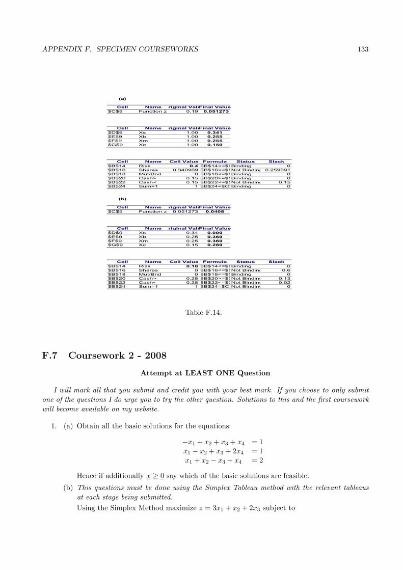
APPENDIX F. SPECIMEN COURSEWORKS 133
(a)
Cell Name riginal ValuFinal Value
$C$5 Function z 0.19 0.051273
Cell Name riginal ValuFinal Value
$D$9 Xs 1.00 0.341
$E$9 Xb 1.00 0.255
$F$9 Xm 1.00 0.255
$G$9 Xc 1.00 0.150
Cell Name Cell Value Formula Status Slack
$B$14 Risk 0.4 $B$14<=$CBinding 0
$B$16 Shares 0.340909 $B$16<=$CNot Binding 0.259091
$B$18 Mut/Bnd 0 $B$18<=$CBinding 0
$B$20 Cash> 0.15 $B$20>=$CBinding 0
$B$22 Cash< 0.15 $B$22<=$CNot Binding 0.15$B$24 Sum=1 1 $B$24=$C$Binding 0
(b)
Cell Name riginal ValuFinal Value
$C$5 Function z 0.051273 0.0408
Cell Name riginal ValuFinal Value
$D$9 Xs 0.34 0.000
$E$9 Xb 0.25 0.360
$F$9 Xm 0.25 0.360
$G$9 Xc 0.15 0.280
Cell Name Cell Value Formula Status Slack
$B$14 Risk 0.18 $B$14<=$CBinding 0
$B$16 Shares 0 $B$16<=$CNot Binding 0.6
$B$18 Mut/Bnd 0 $B$18<=$CBinding 0
$B$20 Cash> 0.28 $B$20>=$CNot Binding 0.13
$B$22 Cash< 0.28 $B$22<=$CNot Binding 0.02$B$24 Sum=1 1 $B$24=$C$Not Binding 0
Table F.14:
F.7 Coursework 2 - 2008
Attempt at LEAST ONE Question
I will mark all that you submit and credit you with your best mark. If you choose to only submitone of the questions I do urge you to try the other question. Solutions to this and the first courseworkwill become available on my website.
1. (a) Obtain all the basic solutions for the equations:
−x1 + x2 + x3 + x4 = 1x1 − x2 + x3 + 2x4 = 1x1 + x2 − x3 + x4 = 2
Hence if additionally x ≥ 0 say which of the basic solutions are feasible.
(b) This questions must be done using the Simplex Tableau method with the relevant tableausat each stage being submitted.Using the Simplex Method maximize z = 3x1 + x2 + 2x3 subject to
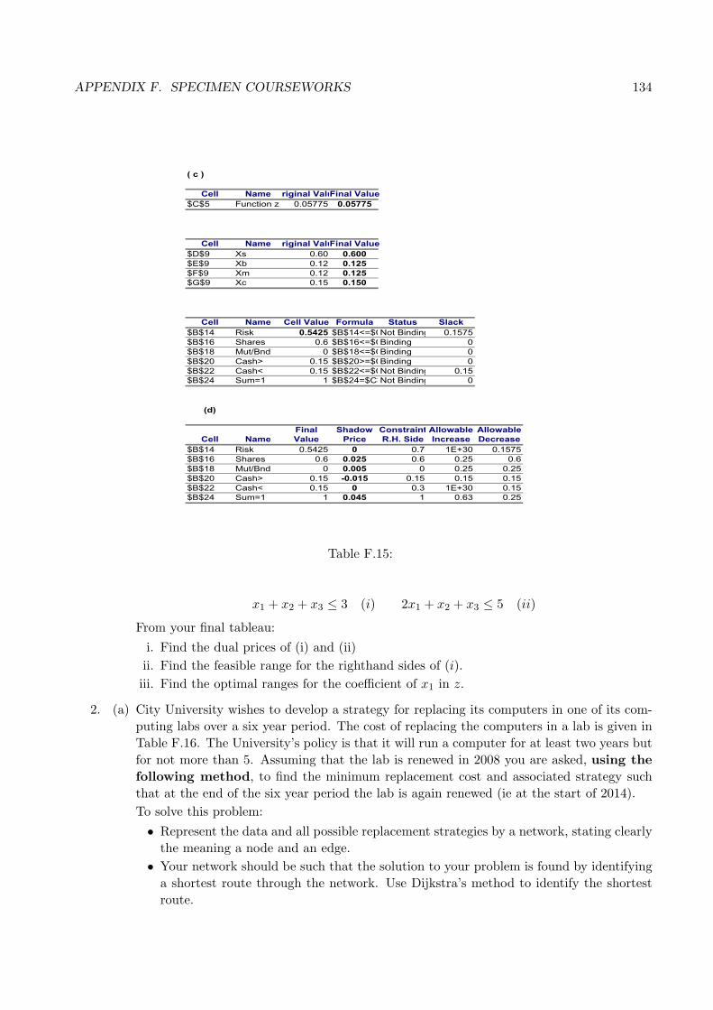
APPENDIX F. SPECIMEN COURSEWORKS 134
( c )
Cell Name riginal ValuFinal Value
$C$5 Function z 0.05775 0.05775
Cell Name riginal ValuFinal Value
$D$9 Xs 0.60 0.600
$E$9 Xb 0.12 0.125
$F$9 Xm 0.12 0.125
$G$9 Xc 0.15 0.150
Cell Name Cell Value Formula Status Slack
$B$14 Risk 0.5425 $B$14<=$CNot Binding 0.1575
$B$16 Shares 0.6 $B$16<=$CBinding 0
$B$18 Mut/Bnd 0 $B$18<=$CBinding 0
$B$20 Cash> 0.15 $B$20>=$CBinding 0
$B$22 Cash< 0.15 $B$22<=$CNot Binding 0.15$B$24 Sum=1 1 $B$24=$C$Not Binding 0
(d)
Final Shadow Constraint Allowable Allowable
Cell Name Value Price R.H. Side Increase Decrease
$B$14 Risk 0.5425 0 0.7 1E+30 0.1575
$B$16 Shares 0.6 0.025 0.6 0.25 0.6
$B$18 Mut/Bnd 0 0.005 0 0.25 0.25
$B$20 Cash> 0.15 -0.015 0.15 0.15 0.15
$B$22 Cash< 0.15 0 0.3 1E+30 0.15$B$24 Sum=1 1 0.045 1 0.63 0.25
Table F.15:
x1 + x2 + x3 ≤ 3 (i) 2x1 + x2 + x3 ≤ 5 (ii)
From your final tableau:i. Find the dual prices of (i) and (ii)ii. Find the feasible range for the righthand sides of (i).iii. Find the optimal ranges for the coefficient of x1 in z.
2. (a) City University wishes to develop a strategy for replacing its computers in one of its com-puting labs over a six year period. The cost of replacing the computers in a lab is given inTable F.16. The University’s policy is that it will run a computer for at least two years butfor not more than 5. Assuming that the lab is renewed in 2008 you are asked, using thefollowing method, to find the minimum replacement cost and associated strategy suchthat at the end of the six year period the lab is again renewed (ie at the start of 2014).To solve this problem:• Represent the data and all possible replacement strategies by a network, stating clearly
the meaning a node and an edge.• Your network should be such that the solution to your problem is found by identifying
a shortest route through the network. Use Dijkstra’s method to identify the shortestroute.

APPENDIX F. SPECIMEN COURSEWORKS 135
lab replaced Replacement cost (£) for given years of useat start of 2 3 4 5
2008 20,000 22,000 23,000 25,0002010 21,000 23,000 24,250 −2011 22,000 23,250 − −2012 23,500 − − −
Table F.16: The figures show the cost of replacing a lab after a given number of year of use as a function ofthe year of its purchase.
(b) In order to distribute its services a cable company wishes to link up eight towns. The costof links between the towns is given in Table F.17. Not all towns can be linked directly toeach other owing to various physical obstructions, hence the table contains blank entries.Also the table is symmetric, indicating that the cost of linking two towns does not dependon the direction in which the cabling is carried out. Cables carry two-way traffic and onlyone cable is necessary to form a direct link between two towns.Draw a network representing the towns and costs and hence using Kruskal’s algorithmconstruct a minimal spanning tree for the network. Write down the minimum cost oflinking the towns and draw the minimal configuration.
Towns 1 2 3 4 5 6 7 81 3 2 12 3 1 43 2 2 34 1 1 2 2 3 3 25 3 2 16 3 1 57 3 5 28 4 2 2
Table F.17: Towns are labeled 1 - 8. The cost of possible links is shown in £10,000
(c) Given a Euclidean space E, define what is meant by:
• L is a line segment of E
• C is a convex subset set of E.• Show that the set of all elements x ∈ E such that for a matrix A and vector b, Ax ≤ b,
is a convex subset of E.
F.8 Coursework 2 - 2008 Solutions
1. (a) You need to row reduce to produce the three standard basis vectors in three of the columnsto start this problem of, and give the first basic solution. I decided to use the first three
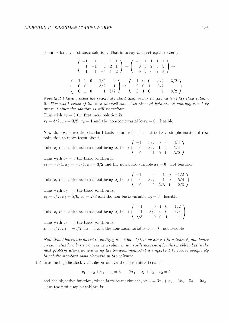
APPENDIX F. SPECIMEN COURSEWORKS 136
columns for my first basic solution. That is to say x4 is set equal to zero.−1 1 1 1 1
1 −1 1 2 11 1 −1 1 2
→
−1 1 1 1 1
0 0 2 3 20 2 0 2 3
→
−1 1 0 −1/2 0
0 0 1 3/2 10 1 0 1 3/2
→
−1 0 0 −3/2 −3/2
0 0 1 3/2 10 1 0 1 3/2
Note that I have created the second standard basis vector in column 3 rather than column2. This was because of the zero in row2-col2. I’ve also not bothered to multiply row 1 byminus 1 since the solution is still immediate.Thus with x4 = 0 the first basic solution is:x1 = 3/2, x2 = 3/2, x3 = 1 and the non-basic variable x4 = 0 feasible
Now that we have the standard basis columns in the matrix its a simple matter of rowreduction to move them about.
Take x2 out of the basic set and bring x4 in →−1 3/2 0 0 3/4
0 −3/2 1 0 −5/40 1 0 1 3/2
Thus with x2 = 0 the basic solution is:x1 = −3/4, x3 = −5/4, x4 = 3/2 and the non-basic variable x2 = 0 not feasible.
Take x3 out of the basic set and bring x2 in →−1 0 1 0 −1/2
0 −3/2 1 0 −5/40 0 2/3 1 2/3
Thus with x3 = 0 the basic solution is:x1 = 1/2, x2 = 5/6, x4 = 2/3 and the non-basic variable x3 = 0 feasible.
Take x1 out of the basic set and bring x3 in →
−1 0 1 0 −1/21 −3/2 0 0 −3/4
2/3 0 0 1 1
Thus with x1 = 0 the basic solution is:x2 = 1/2, x3 = −1/2, x4 = 1 and the non-basic variable x1 = 0 not feasible.
Note that I haven’t bothered to multiply row 2 by −2/3 to create a 1 in column 2, and hencecreate a standard basis element as a column...not really necessary for this problem but in thenext problem where we are using the Simplex method it is important to reduce completelyto get the standard basis elements in the columns
(b) Introducing the slack variables s1 and s2 the constraints become:
x1 + x2 + x3 + s1 = 3 2x1 + x2 + x3 + s2 = 5
and the objective function, which is to be maximized, is: z = 3x1 + x2 + 2x3 + 0s1 + 0s2
Thus the first simplex tableau is:

APPENDIX F. SPECIMEN COURSEWORKS 137
x1 x2 x3 s1 s2 d da
Basic Var cj 3 1 2 0 0 ratio
s1 0 1 1 1 1 0 3 3s2 0 2 1 1 0 1 5 [5/2]zj 0 0 0 0 0 z =∆z [3] 1 2 0 0 0
Table F.18: Bring in x1, since 3 is the largest positive number on the last row. Take out s2 since 5/2is the smallest non-negative number in the ratio column.
Since we are bringing in x1 and taking out s2 row reduce to make the first column of the
coefficient matrix inside the double lining equal to(
01
).
x1 x2 x3 s1 s2 d da
Basic Var cj 3 1 2 0 0 ratio
s1 0 0 1/2 1/2 1 −1/2 1/2 [1]x1 3 1 1/2 1/2 0 1/2 5/2 5zj 3 3/2 3/2 0 3/2 z =∆z 0 −1/2 [1/2] 0 −3/2 15/2
Table F.19: Bring in x3, since 1/2 is the largest positive number on the last row. Take out s1 since 1is the smallest non-negative number in the ratio column.
Since we are bringing in x3 and taking out s1 row reduce to make the third column of the
coefficient matrix inside the double lining equal to(
10
).
x1 x2 x3 s1 s2 d da
Basic Var cj 3 1 2 0 0 ratio
x3 2 0 1 1 2 −1 1x1 3 1 0 0 −1 1 2zj 3 2 2 (1) (1) z =∆z 0 −1 0 −1 −1 8
Table F.20: Bring in x3, since 1/2 is the largest positive number on the last row. Take out s1 since 1is the smallest non-negative number in the ratio column.
Since the final row consists of zeros and negative numbers and this is a maximizationproblem the tableau is optimal.The optimal solution is x1 = 2, x2 = 0 and x3 = 1 with a maximum z equal to 8.
i. The dual variables are in the penultimate row in the columns corresponding to theslack variables and if present the artificial variables. Thus in this problem the dualvariable are both equal to 1.

APPENDIX F. SPECIMEN COURSEWORKS 138
ii. The feasible range of the righthand side of the first constraint is given by solving:(
12
)+
(2 −1−1 1
)(δ0
)≥ 0 ⇒ −1/2 ≤ δ ≤ 2
Thus since the original righthand side of the first constraint is 3 the feasible range forthis value is [5/2, 5].
iii. To find the optimal range for the coefficient of x1 in the objective function we use theoptimal tableau this coefficient replaced with α.
x1 x2 x3 s1 s2 d da
Basic Var cj α 1 2 0 0 ratio
x3 2 0 1 1 2 −1 1x1 α 1 0 0 −1 1 2zj α 2 2 4− α −2 + α z =∆z 0 −1 0 α− 4 2− α 2 + 2α
Table F.21:
For the table to remain optimal the final row must remain zero or negative, thus;
α− 4 ≤ 0 ⇒ α ≤ 4 2− α ≤ 0 ⇒ 2 ≤ α ⇒ 2 ≤ α ≤ 4
Thus the optimal range for the x1 coefficient in the objective function is 2 ≤ α ≤ 4.
2. (a) Construct a network as follows. Each vertex(node) contains the year of purchase of a newcar. Each edge contains the cost of replacing a car determined by the vertices at its ends.This network is shown in Figure F.3 and as can be seen the vertex (13) is redundant sinceit is not possible to move to the final vertex (14) due to the lab having to be kept for atleast two years. However I have left this in my diagram, you may have been smart andeliminated it right from the start.Dijkstra’s MethodThe method labels the nodes [distance back to (08),previous node] and underlines a labelonce it becomes permanent.
(i) Label (08) with [0,8](ii) Add temporary labels to all nodes directly connected to (08). ie Add the labels: [20,8],
[22,8], [25,8] and [23,8](iii) Make the smallest temporary label, [20,8] at node(10), permanent and denote as [20,8].(iv) Add temporary labels to all vertices directly connected to node(10) that either have no
label or have a temporary label with distance back to (08) greater than the associatededge value + distance on node(10.) There is only one such node, and that is node(14).Label node(14) as [44.25,10].
(v) Make the smallest temporary label, [22,8] at node(11), permanent and denote as [22,8].(vi) Add temporary label as before to all nodes directly linked to node(11). There are none
to add, since the temporary labels on nodes(13) and (14) have a shorter distance backto node(08) than via node(11).

APPENDIX F. SPECIMEN COURSEWORKS 139
(vii) Make the smallest temporary label, [23,8] at node(12), permanent.(viii) Add temporary labels as before to all nodes directly linked to node(12). There are
none to add.(ix) Make the smallest temporary label, [25,8] at node(13), permanent.(x) No nodes connected directly to node(13)(xi) Make the smallest temporary node, [44.25,10] at node(14) permanent.
Since we now have a permanent label on the node to which we wish to find theshortest route, the process stops.In this example it would have stopped anyway since there were no temporary labels, or nodeswithout labels, to which to apply the updating process.
08
10
12
13
11
14
µ
*
s
j
z
:R
6
?
:
20,000
22,000
23,000
25,000
24,250
23,250
23,00021,000
23,500
22,000
[0,8]
[20,8]
[25,8]
[22,8]
[23,8]
[44.25,10]
Figure F.3: Each vertex is named with the year of purchase of a new car. The edges are labelled withthe cost of replacement. The labels on each vertex are from Dijkstra and indicate the distance back tovertex 08 measured in thousands followed by the name of the previous node.
The optimal solution is to replace after 2 year and then 4 years at a cost of £44,250.
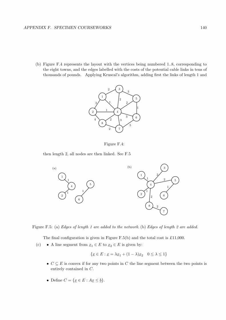
APPENDIX F. SPECIMEN COURSEWORKS 140
(b) Figure F.4 represents the layout with the vertices being numbered 1..8, corresponding tothe eight towns, and the edges labelled with the costs of the potential cable links in tens ofthousands of pounds. Applying Kruscal’s algorithm, adding first the links of length 1 and
1
2
3
8
7
6
5
4
1
11
2
22
2
2
3
33
3
4
5
Figure F.4:
then length 2, all nodes are then linked. See F.5
(a)
1
2
4
6
5
1
11
(b)
1
2
4
6
51
1
1
3
8
2
2
2
7
2
Figure F.5: (a) Edges of length 1 are added to the network. (b) Edges of length 2 are added.
The final configuration is given in Figure F.5(b) and the total cost is £11,000.
(c) • A line segment from x1 ∈ E to x2 ∈ E is given by:
{x ∈ E : x = λx1 + (1− λ)x2 0 ≤ λ ≤ 1}
• C ⊆ E is convex if for any two points in C the line segment between the two points isentirely contained in C.
• Define C = {x ∈ E : Ax ≤ b}.

APPENDIX F. SPECIMEN COURSEWORKS 141
Let x1 and x2 be any two points in C. That is to say
Ax1 ≤ b and Ax2 ≤ b
Construct the line segment between the two points and show that all points on it arein C.
x = λx2 + (1− λ)x1 ⇒ Ax + λAx2 + (1− λ)Ax1 ≤ λb + (1− λ)b = b
Thus all points x on the line satisfy Ax ≤ b and are therefore in C.C is therefore convex.