probability, random processes and inference - cic …pescamilla/prpi/slides/prpi_2.pdf ·...

INSTITUTO POLITÉCNICO NACIONAL CENTRO DE INVESTIGACION EN COMPUTACION

Probability, Random Processes and Inference

Dr. Ponciano Jorge Escamilla Ambrosio [email protected]

http://www.cic.ipn.mx/~pescamilla/

Laboratorio de

Ciberseguridad

CIC

2

Course Content

1.3. Discrete Random Variables

1.3.1. Basic Concepts

1.3.2. Probability Mass Functions

1.3.3. Functions of Random Variables

1.3.4. Expectation and Variance

1.3.5. Joint PMFs of Multiple Random Variables

1.3.6. Conditioning

1.3.7. Independence

CIC

3

The Modelling Process

• A model is an approximate

representation of a physical

situation.

• A useful model explains all

relevant aspects of a given

situation.

• Mathematical models are used

when the observational

phenomenon has measurable

properties.

• The model is used to predict the

outcome of the experiment, and

these predictions are compared with

the actual observations that result

when the experiment is carried out.

CIC

The predictions of a mathematical model should be

treated as hypothetical until the model has been

validated through a comparison with experimental

measurements.

What if the model cannot be validated experimentally

because the real system does not exist?

Computer simulation models play a useful role in this

situation by presenting an alternative means of

predicting system behavior, and thus a means of

checking the predictions made by a mathematical

model.

4

Computer Simulation Models

CIC

A computer simulation model consists of a

computer program that simulates or mimics the

dynamics of a system.

Simulation models are capable of representing

systems in greater detail than mathematical

models.

they tend to be less flexible and usually require more

computation time than mathematical models.

5

Computer Simulation Models

CIC

In deterministic models the conditions under which an experiment

is carried out determine the exact outcome of the experiment.

In deterministic mathematical models, the solution of a set of

mathematical equations specifies the exact outcome of the

experiment.

Circuit theory is an example of a deterministic mathematical model.

Kirchhoff’s voltage and current laws, Ohm’s law.

If an experiment involving the measurement of a set of voltages is

repeated a number of times under the same conditions, circuit

theory predicts that the observations will always be exactly the

same.

6

Deterministic Models

CIC

Many systems of interest involve phenomena that

exhibit unpredictable variation and randomness.

We define a random experiment to be an

experiment in which the outcome varies in an

unpredictable fashion when the experiment is

repeated under the same conditions.

Deterministic models are not appropriate for

random experiments.

7

Probability Models

CIC

Example of a random experiment

8

Probability Models

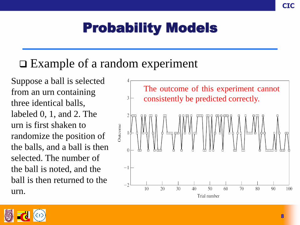
Suppose a ball is selected

from an urn containing

three identical balls,

labeled 0, 1, and 2. The

urn is first shaken to

randomize the position of

the balls, and a ball is then

selected. The number of

the ball is noted, and the

ball is then returned to the

urn.

The outcome of this experiment cannot

consistently be predicted correctly.

CIC

Random variable. Given an experiment with sample

space S (the corresponding set of possible

outcomes), a random variable (r.v.) is a function

from the sample space S to the real numbers ℝ.

A random variable X assigns a numerical value X(s)

to each possible outcome s of the experiment.

The randomness comes from the fact that we have a

random experiment (with probabilities described by

the probability function P); the mapping itself is

deterministic.

9

Random Variables

CIC

10

Random Variables

Real number line

ℝ

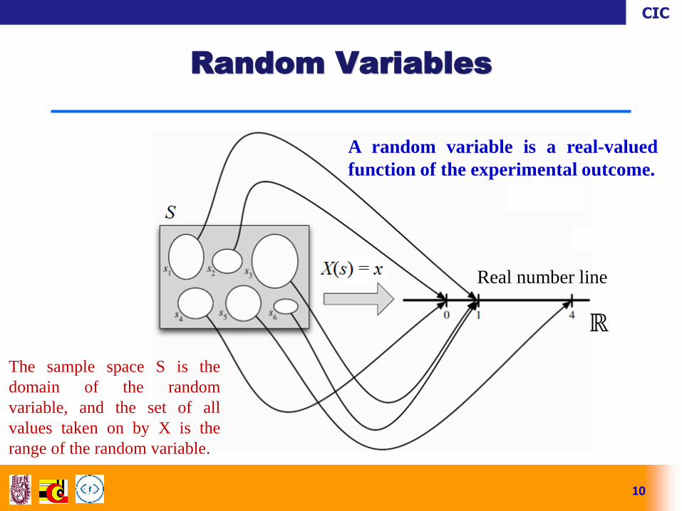
A random variable is a real-valued

function of the experimental outcome.

The sample space S is the

domain of the random

variable, and the set of all

values taken on by X is the

range of the random variable.

CIC

11

Random Variables

CIC

12

Random Variables

CIC

Random variables are usually denoted by capital letters from

the end of the alphabet, such as X, Y, Z.

Related sets are denoted like {s : X(s) = x}, {s : X(s) ≤ x}, and

{s : X(s) ∈ I }, for any number x and any interval I, are events

in S.

They are usually abbreviated as {X = x}, {X ≤ x}, and {X ∈ I }

and have probabilities associated with them.

The assignment of probabilities to all such events, for a given

random variable X, is called the probability distribution of X.

In the notation for such probabilities, it is usual to write

P(X = x), rather than P({X = x}).

13

Random Variables

CIC

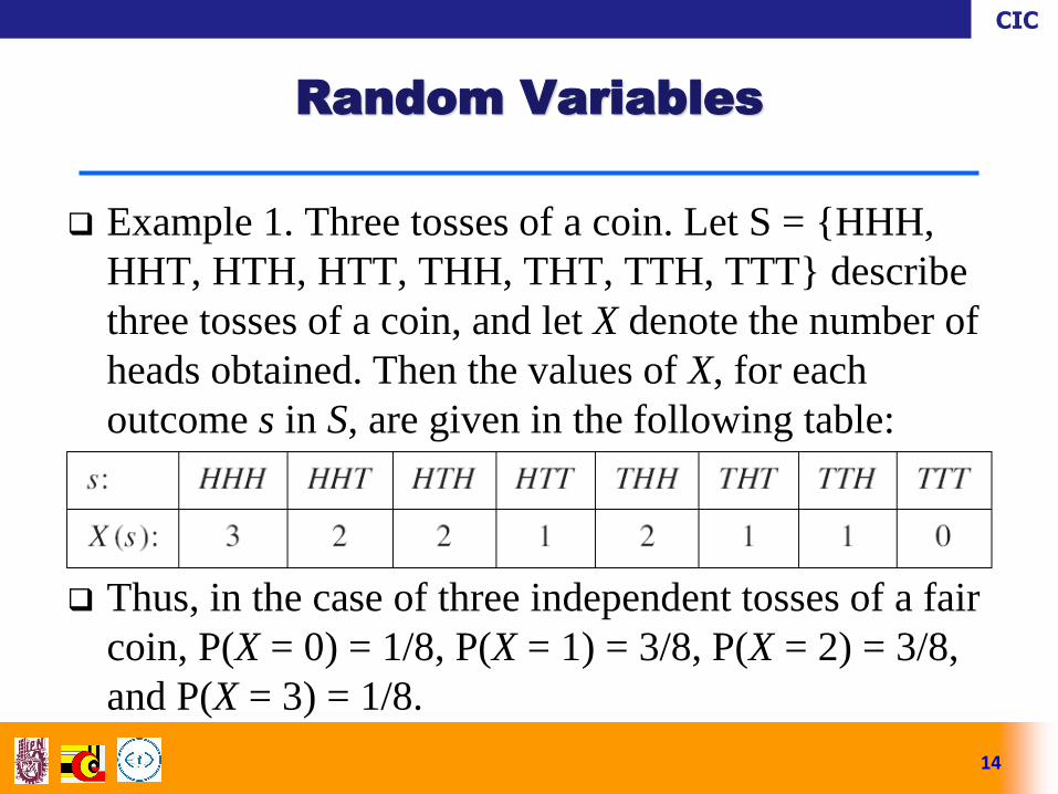
Example 1. Three tosses of a coin. Let S = {HHH,

HHT, HTH, HTT, THH, THT, TTH, TTT} describe

three tosses of a coin, and let X denote the number of

heads obtained. Then the values of X, for each

outcome s in S, are given in the following table:

Thus, in the case of three independent tosses of a fair

coin, P(X = 0) = 1/8, P(X = 1) = 3/8, P(X = 2) = 3/8,

and P(X = 3) = 1/8.

14

Random Variables

CIC

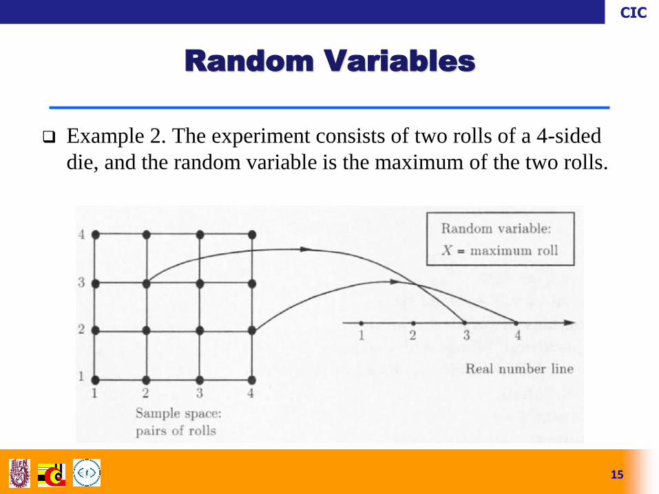
Example 2. The experiment consists of two rolls of a 4-sided

die, and the random variable is the maximum of the two rolls.

15

Random Variables

CIC

16

Examples of Random Variables

CIC

17

Random Variables

CIC

18

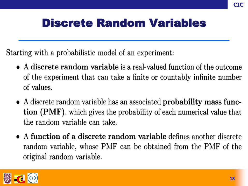
Discrete Random Variables

CIC

(Blitzstein and Hwang, 2015). A random variable

X is said to be discrete if there is a finite list of

values a1, a2, . . . ,an or an infinite list of values

a1, a2, . . . such that P(X = aj for some j) = 1. If X

is a discrete r.v., then the finite or countably

infinite set of values x such that P(X = x) > 0 is

called the support of X.

19


CIC

Given a random variable, we would like to be

able to describe its behavior using the language

of probability.

For example, we might want to answer questions

about the probability that the r.v. will fall into a

given range:

If M is the number of major earthquakes in Mexico

City in the next five years, what is the probability that

M equals 0?

20


CIC

The most important way to characterise a random

variable is through the probabilities of the values

that it can take.

For a discrete random variable X, these are

captured by the probability mass function (PMF)

of X, denoted as pX.

21

Probability Mass Function

CIC

The probability mass function (PMF) of a

discrete r.v. X is the function pX given by pX(x) =

P(X = x).

Note that this is positive if x is in the support of X,

and 0 otherwise.

In particular, if x is any possible value of X, the

probability mass of x, denoted pX(x) is the

probability of the event {X = x} consisting of all

outcomes that give rise to a value of X equal to x:

pX(x) = P(X = x).

22


CIC

In writing P(X = x), we are using X = x to denote

an event, consisting of all outcomes s to which X

assigns the number x.

This event is also written as {X = x}; formally,

{X = x} is defined as {s S : X(s) = x}, but

writing {X = x} is shorter and more intuitive.

23


CIC

Example 3. (Coin two tosses). Consider an

experiment where we toss a fair coin twice. The

sample space consists of four possible outcomes:

S = {HH, HT, TH, TT}.

Let X be the number of Heads. This is a random

variable with possible values 0, 1, and 2. Viewed as a

function, X assigns the value 2 to the outcome HH, 1 to

the outcomes HT and TH, and 0 to the outcome TT.

That is, X(HH) = 2, X(HT) = X(TH) = 1, X(TT) = 0.

Find the PMFs of the random variable X.

24


CIC

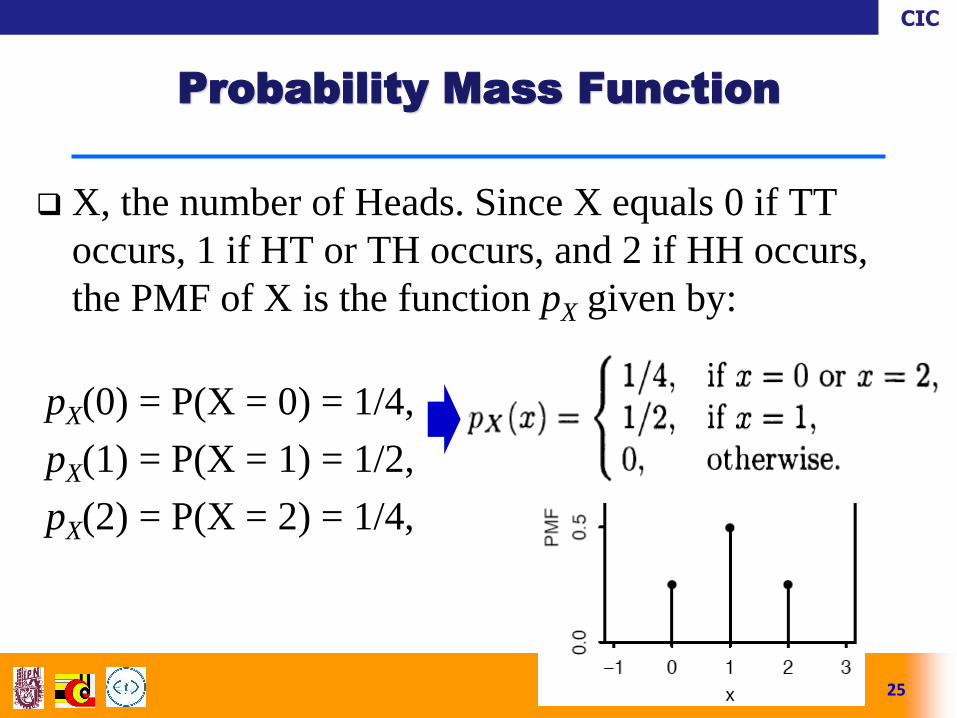
X, the number of Heads. Since X equals 0 if TT

occurs, 1 if HT or TH occurs, and 2 if HH occurs,

the PMF of X is the function pX given by:

pX(0) = P(X = 0) = 1/4,

pX(1) = P(X = 1) = 1/2,

pX(2) = P(X = 2) = 1/4,

25


CIC

Example 4. Three tosses of a coin. Let X be the

number of heads obtained in three independent

tosses of a fair coin, as in the previous example.

Find the PMF of X.

26


CIC

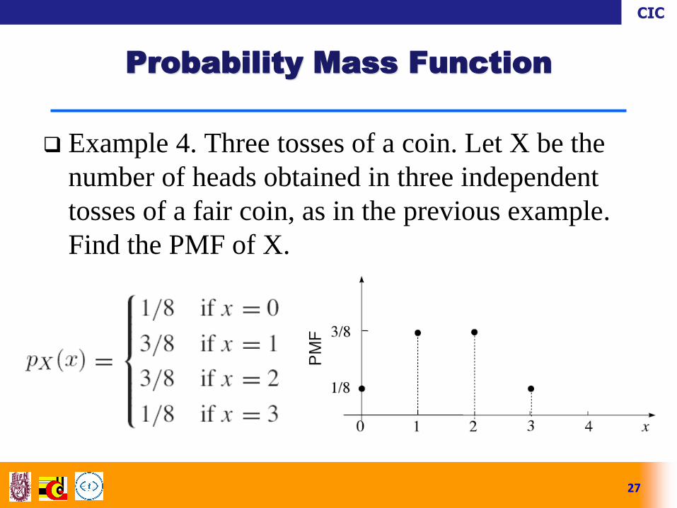
Example 4. Three tosses of a coin. Let X be the

number of heads obtained in three independent

tosses of a fair coin, as in the previous example.

Find the PMF of X.

27


CIC

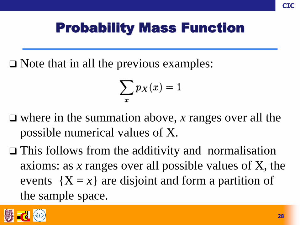
Note that in all the previous examples:

where in the summation above, x ranges over all the

possible numerical values of X.

This follows from the additivity and normalisation

axioms: as x ranges over all possible values of X, the

events {X = x} are disjoint and form a partition of

the sample space.

28


CIC

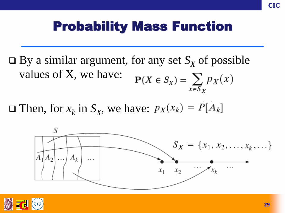
By a similar argument, for any set SX of possible

values of X, we have:

Then, for xk in SX, we have:

29


CIC

The events A1, A2 , … form a partition of S. These events

are disjoint. Let j ≠ k, then:

since each ζ is mapped into one and only one value in SX .

30


CIC

31


Next we show that S is the union of the Ak’s. Every ζ in S

is mapped into some xk so that every ζ belongs to an

event Ak in the partition. Therefore:

All events involving the random variable X can be

expressed as the union of events Ak’s. For example,

suppose we are interested in the event X in B = {x2, x5},

then:

CIC

32


The PMF pX(x) satisfies three properties that

provide all the information required to calculate

probabilities for events involving the discrete

random variable X:

CIC

33


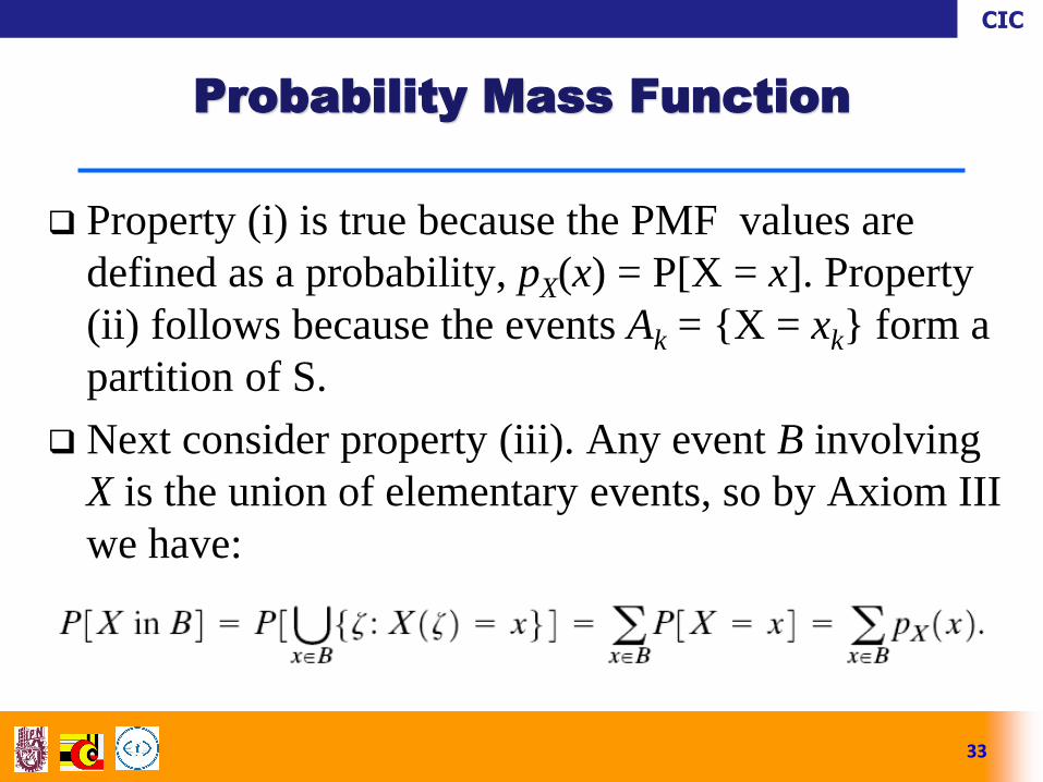
Property (i) is true because the PMF values are

defined as a probability, pX(x) = P[X = x]. Property

(ii) follows because the events Ak = {X = xk} form a

partition of S.

Next consider property (iii). Any event B involving

X is the union of elementary events, so by Axiom III

we have:

CIC

The PMF of X gives us the probabilities for all the

elementary events from SX.

The probability of any subset of SX is obtained from the

sum of the corresponding elementary events.

In fact we have everything required to specify a

probability law for the outcomes in SX .

If we are only interested in events concerning X, then

we can forget about the underlying random experiment

and its associated probability law and just work with SX

and the PMF of X.

34


CIC

For example, if X is the number of heads

obtained in two independent tosses of a fair coin,

then the probability of at least on head is:

Recall that:

35


CIC

36


CIC

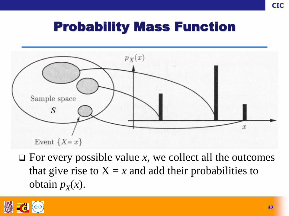
For every possible value x, we collect all the outcomes

that give rise to X = x and add their probabilities to

obtain pX(x).

37


CIC

38


CIC

The cumulative distribution function (CDF) of a

random variable (r.v.) X is a function FX(x)

mapping ℝ → ℝ and is defined by FX(x) = P{s

S : X(s) x}. The argument s is usually omitted

for brevity, so FX(x) = P{X x}.

The CDF FX(x) is non-decreasing with x and

must satisfy:

limx→− FX(x) = 0 and limx→ FX(x) = 1.

39

Cumulative Distribution Function

The cumulative distribution function is often referred to simply as the distribution function.

CIC

Example 5. Three tosses of a coin. Given the

PMF of X obtained in Example 4, obtain the

CDF of X.

40


CIC

The CDF of a discrete r.v. is a “staircase

function,” staying constant between the possible

sample values and having a jump of magnitude

pX(xi) at each sample value xi.

The PMF and the CDF each specify the other for

discrete r.v.’s.

41


CIC

A random variable X is called a Bernoulli random

variable with parameter p, if it has two possible values,

0 and 1, with P(X = 1) = p and P(X = 0) = 1 − p = q,

where p is any number from the interval [0, 1].

An experiment whose outcome is a Bernoulli random

variable is called a Bernoulli trial process.

A Bernoulli r.v. has a Bernoulli distribution referred to

as X Bern(p). The symbol is read “is distributed

as”.

42

Bernoulli Random Variables

CIC

This number p in Bern(p) is called the parameter of the

distribution; it determines which specific Bernoulli distribution

we have.

There is not just one Bernoulli distribution, but rather a family of

Bernoulli distributions, indexed by p.

The indicator random variable of an event A is the r.v. which

equals 1 if A occurs and 0 otherwise. We will denote the indicator

r.v. of A by IA or I(A). Note that IA Bern(p) with p = P(A).

The parameter p is often called the success probability of the

Bern(p) distribution.

43


CIC

Example 6. Consider the toss of a coin, which

comes up head with probability p, and tail with

probability 1 ˗ p, The Bernoulli random variable

takes the two values 1 and 0, depending on

whether the outcome is a head or a tail:

Its PMF is:

44


CIC

In practice, for its simplicity the Bernoulli random

variable is used to model generic probabilistic

situations with just two outcomes, such as:

The state of a telephone at a given time that can be either

free or busy.

A person who can be either healthy or sick with a certain

disease.

The preference of a person who can be either for or

against a certain political candidate.

45


CIC

A Bernoulli trials process is a sequence of n chance

experiments such that:

1. Each experiment has two possible outcomes, which we

may call success and failure.

2. The probability p of success on each experiment is the

same for each experiment, and this probability is not

affected by any knowledge of previous outcomes. The

probability q of failure is given by q = 1 − p.

46

Bernoulli trial process

CIC

To analyze a Bernoulli trials process, choose as the sample space a binary tree

and assign a probability distribution to the paths in this tree.

Define X to be the random variable which represents the outcome of the

process, i.e., an ordered triple of S’s and F’s.

Let the outcome of the ith trial be denoted by the random variable Xi, with

distribution function mi.

An outcome for the entire experiment will be a path through the tree. For

example, 3 represents the outcomes SFS.

This suggests assigning probability pqp to the outcome 3 . More generally, we

assign a distribution function m() for paths by defining m() to be the

product of the branch probabilities along the path .

Thus, the probability that the three events S on the first trial, F on the second

trial, and S on the third trial occur is the product of the probabilities for the

individual events.

47

Bernoulli trial process analysis

CIC

48

Bernoulli trial process analysis

CIC

Suppose that n independent Bernoulli trials are

performed, each with the same success probability p,

and failure probability q = 1 ˗ p . Let X be the number

of successes. Given this, X is called a binomial

random variable with parameters n and p.

The PMF of X consists of the binomial probabilities

calculated as:

49

Binomial Random Variable

CIC

Example 7. Let the probability of n Bernoulli trials

having exactly k successes be denotes by b(n, p, k).

Let us calculate the particular value b(3, p, 2) from

our tree measure. We see that there are three paths

which have exactly two successes and one failure,

namely 2, 3, and 5.

Each of these paths has the same probability p2q. Thus

b(3, p, 2) = 3 p2q.

50


CIC

Considering all possible numbers of successes we

have:

51


CIC

Carrying out a tree measure for n experiments and

determining b(n, p, k) for the general case of n

Bernoulli trials, the probability of exactly k successes

is:

52


CIC

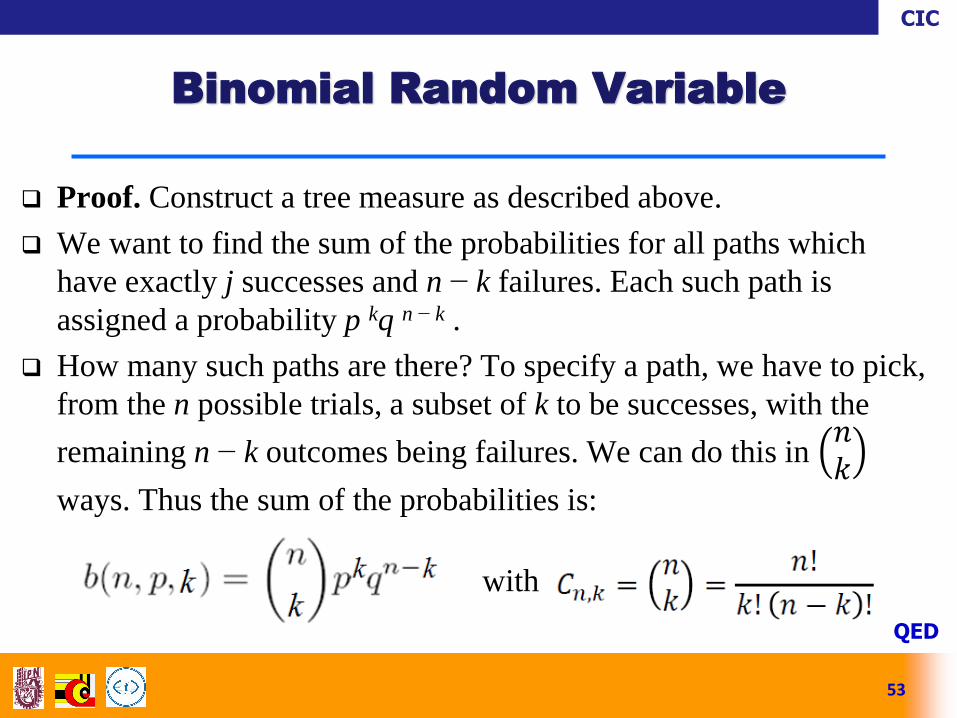
Proof. Construct a tree measure as described above.

We want to find the sum of the probabilities for all paths which

have exactly j successes and n − k failures. Each such path is

assigned a probability p kq n − k .

How many such paths are there? To specify a path, we have to pick,

from the n possible trials, a subset of k to be successes, with the

remaining n − k outcomes being failures. We can do this in 𝑛𝑘

ways. Thus the sum of the probabilities is:

53


QED

with

CIC

Example 8. A fair coin is tossed six times. What

is the probability that exactly three heads turn

up?

54


CIC

Example 8. A fair coin is tossed six times. What

is the probability that exactly three heads turn

up?

55


CIC

Example 9. A die is rolled four times. What is the

probability that we obtain exactly one 6?

56


CIC

Example 9. A die is rolled four times. What is the

probability that we obtain exactly one 6?

57


CIC

58

Binomial PMF for various values

of n and p

CIC

Let n be a positive integer, and let p be a real number

between 0 and 1. Let X be the random variable which

counts the number of successes in a Bernoulli trials

process with parameters n and p. Then the

distribution of X is called the binomial distribution

function with parameters n and p.

We write X Bin(n, p) to mean that X has the

binomial distribution function with parameters n and

p.

59

Binomial Distribution Function

CIC

The binomial distribution function of a binomial

random variable is given by:

60

Binomial Distribution Function

CIC

Suppose that we repeatedly and independently toss a coin

with probability of head equal to p, where 0 p 1.

The geometric random variable is the number X of tosses

needed for a head to come up for the first time.

Its PMF is given by:

Since (1 p)k1p is the probability of the sequence consisting

of k 1 successive tails followed by a head.

61

Geometric Random Variable

CIC

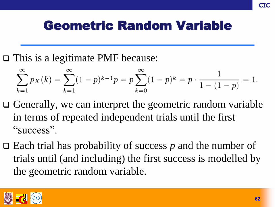
This is a legitimate PMF because:

Generally, we can interpret the geometric random variable

in terms of repeated independent trials until the first

“success”.

Each trial has probability of success p and the number of

trials until (and including) the first success is modelled by

the geometric random variable.

62


CIC

Example 9. Message transmission. Let X be the number

of times a message needs to be transmitted until it

arrives correctly at its destination. Find the PMF of X.

Find the probability that X is an even number.

63


CIC

64


CIC

The PMF of a geometric random variable decreases as a

geometric progression with parameter 1 p.

65


CIC

A Poisson random variable has a PMF given by:

where is a positive parameter characterising

the PMF.

This is a legitimate PMF because:

66

Poisson Random Variable

CIC

If 1, then the PMF is monotonically decreasing

with k, while if 1, then the PMF first increases

and then decreases.

67


CIC

The Poisson PMF with parameter is a good

approximation for a binomial PMF with the

parameters n and p. i.e.:

provided = np, n is very large, and p is very

small.

68


CIC

Example 10. Let n = 100 and p = 0.01.

Calculate the probability of k = 5 successes in n = 100

trials using the binomial PMF.

Calculate the Poisson PMF with = np and compare

results.

69


CIC

70


CIC

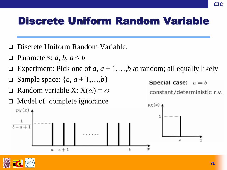
Discrete Uniform Random Variable.

Parameters: a, b, a b

Experiment: Pick one of a, a + 1,…,b at random; all equally likely

Sample space: {a, a + 1,…,b}

Random variable X: X() =

Model of: complete ignorance

71

Discrete Uniform Random Variable

CIC

Discrete Uniform Random Variable. Let C be a

finite, nonempty set of numbers. Choose one of

these numbers uniformly at random (i.e., all

values in C are equally likely). Call the chosen

number X. Then X is called discrete uniform

random variable and have the Discrete Uniform

distribution with parameter C; we denote this by

X DUnif(C).

72


CIC

The PMF of X DUnif(C) is:

for x C (and 0 otherwise), since a PMF must sum

to 1. As with questions based on the naive definition

of probability, questions based on a Discrete

Uniform distribution reduce to counting problems.

Specifically, for X DUnif(C) and any A C, we

have:

73


CIC

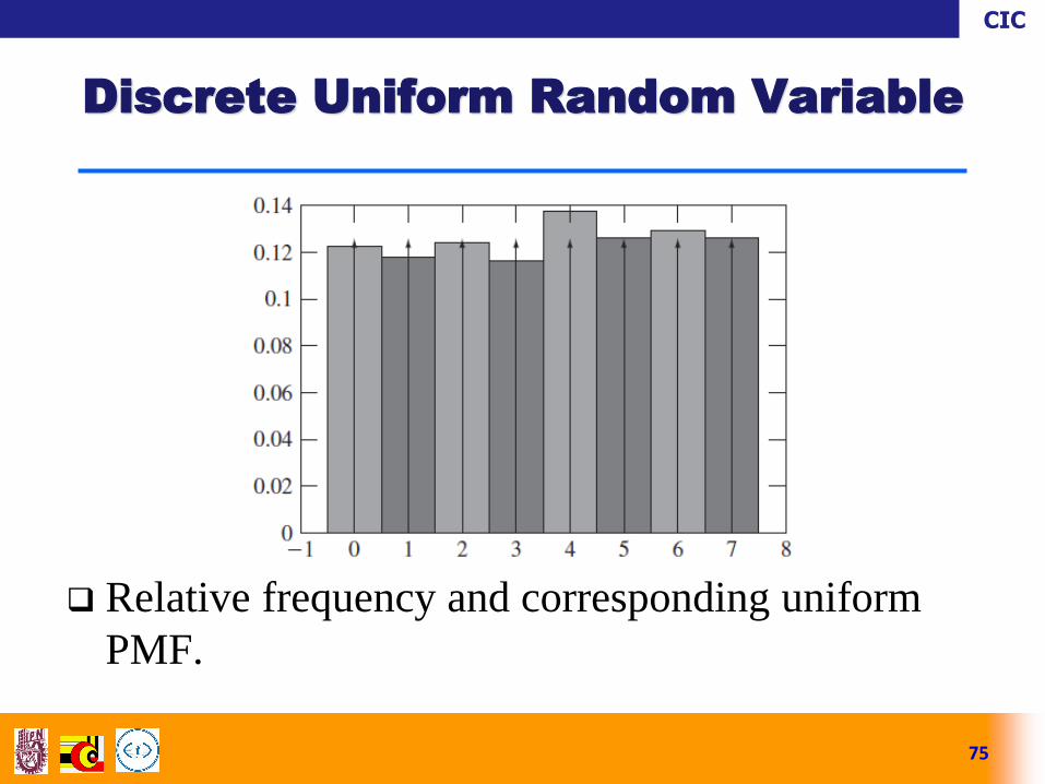
Example 11. Let’s consider the relationship

between relative frequencies and the PMF pX(xk).

Suppose we perform n independent repetitions to

obtain n observations of the discrete random

variable X. Let Nk(n) be the number of times the

event X = xk occurs and let be fk(n) = Nk(n)/n the

corresponding relative frequency. As n becomes

large we expect that fk(n) pX(xk). Therefore the

graph of relative frequencies should approach the

graph of the PMF.

74


CIC

75


Relative frequency and corresponding uniform

PMF.

CIC

For an experiment with sample space S, an r.v. X,

and a function ɡ : ℝ → ℝ, ɡ(X) is the r.v. that

maps s to ɡ(X(s)) for all s S.

A function of a random variable is a random

variable.

If X is a random variable, then X2, eX, and sin(X) are

also random variables, as is ɡ(X) for any function

ɡ : ℝ → ℝ.

76

Functions of Random Variables

CIC

77


Example 1. Taking ɡ(x) = 𝑥, ɡ(x) is the

composition of the function X and ɡ

“First apply X, then apply ɡ”

CIC

78


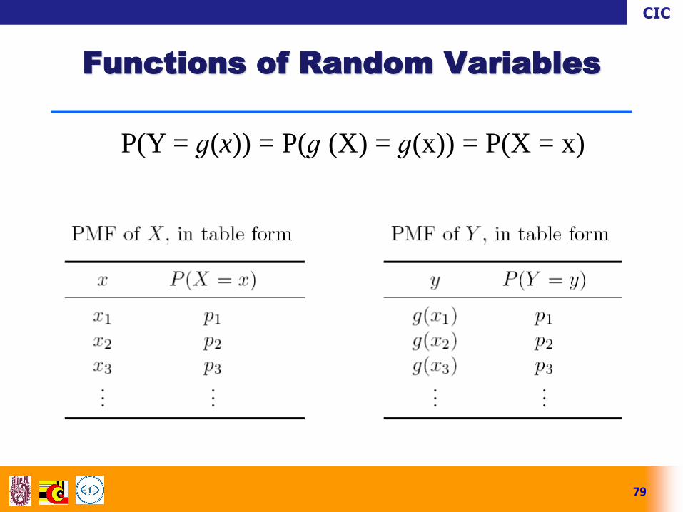
Given a discrete r.v. X with a known PMF, how

can we find the PMF of Y = ɡ(X)?

In the case where ɡ is a one-to-one function, the

support of Y is the set of all ɡ(x) with x in the support

of X, and:

P(Y = ɡ(x)) = P(ɡ(X) = ɡ(x)) = P(X = x)

CIC

79


P(Y = ɡ(x)) = P(ɡ (X) = ɡ(x)) = P(X = x)

CIC

A strategy for finding the PMF of an r.v. with an

unfamiliar distribution:

try to express the r.v. as a one-to-one function of an r.v.

with a known distribution.

Example 2. A particle moves n steps on a number

line. The particle starts at 0, and at each step it

moves 1 unit to the right or to the left, with equal

probabilities. Assume all steps are independent. Let

Y be the particle’s position after n steps. Find the

PMF of Y.

80


CIC

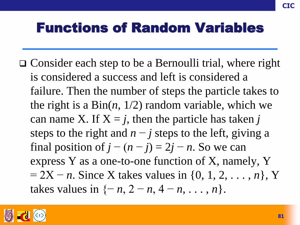
Consider each step to be a Bernoulli trial, where right

is considered a success and left is considered a

failure. Then the number of steps the particle takes to

the right is a Bin(n, 1/2) random variable, which we

can name X. If X = j, then the particle has taken j

steps to the right and n − j steps to the left, giving a

final position of j − (n − j) = 2j − n. So we can

express Y as a one-to-one function of X, namely, Y

= 2X − n. Since X takes values in {0, 1, 2, . . . , n}, Y

takes values in {− n, 2 − n, 4 − n, . . . , n}.

81


CIC

The PMF of Y can then be found from the PMF

of X:

P(Y = k) = P(2X − n = k) = P(X = (n + k)/2) = 𝑛

𝑛+𝑘

2

1

2

𝑛

if k is an integer between − n and n (inclusive) such that n + k is

an even number.

If ɡ is not one-to-one, then for a given y, there may be

multiple values of x such that ɡ(x) = y. To compute P(ɡ(X) =

y), we need to sum up the probabilities of X taking on any of

these candidate values of x.

82


CIC

(PMF of ɡ(X)). Let X be a discrete r.v. and

ɡ : ℝ → ℝ. Then the support of ɡ(X) is the set of

all y such that ɡ(x) = y for at least one x in the

support of X, and the PMF of ɡ(X) is:

for all y in the support of ɡ(X).

83


CIC

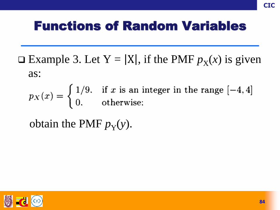
Example 3. Let Y = X , if the PMF pX(x) is given

as:

obtain the PMF pY(y).

84


CIC

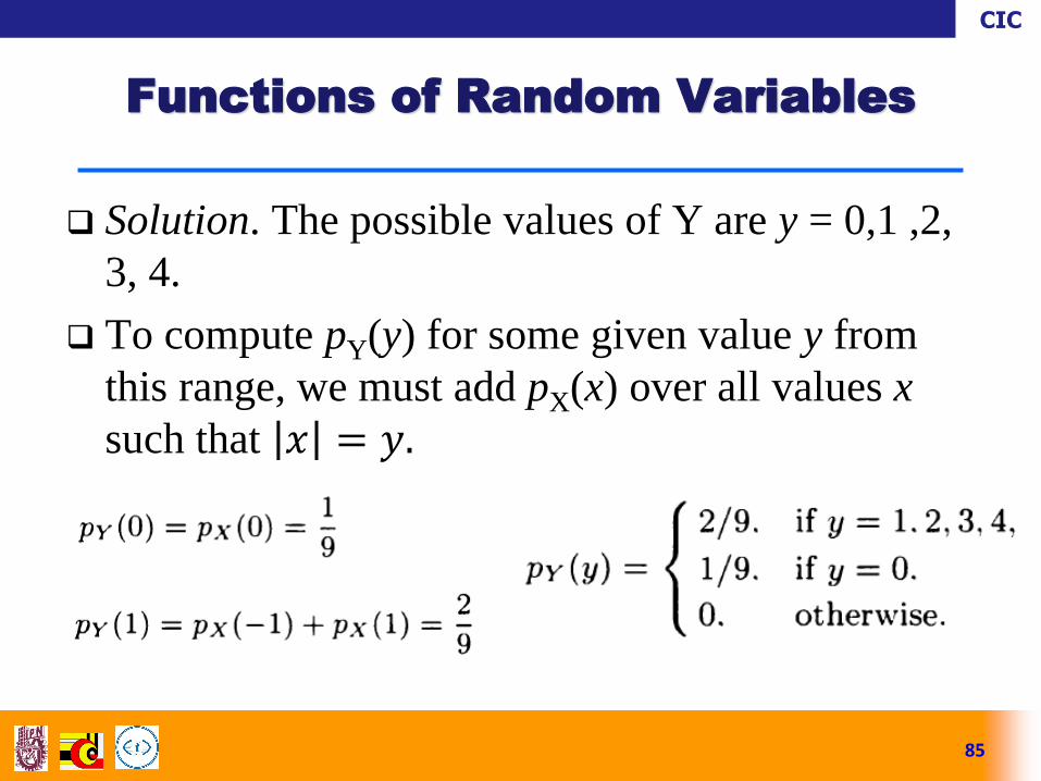
Solution. The possible values of Y are y = 0,1 ,2,

3, 4.

To compute pY(y) for some given value y from

this range, we must add pX(x) over all values x

such that 𝑥 = 𝑦.

85


CIC

Solution

86


CIC

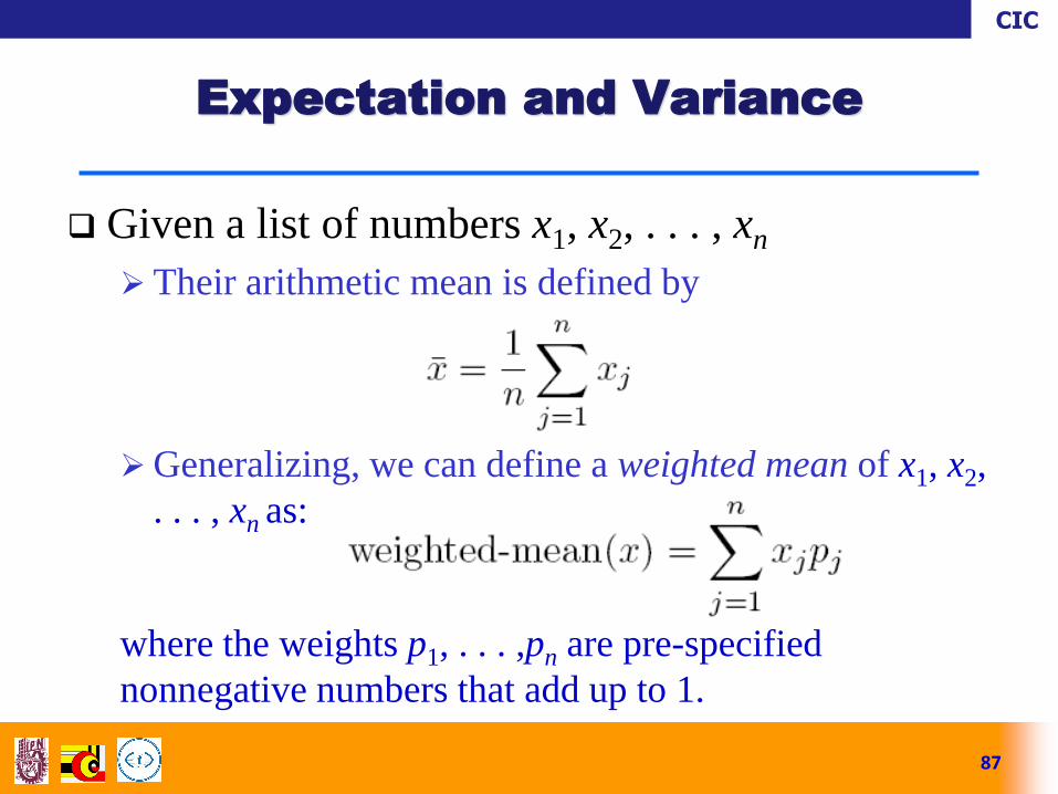
Given a list of numbers x1, x2, . . . , xn

Their arithmetic mean is defined by

Generalizing, we can define a weighted mean of x1, x2,

. . . , xn as:

where the weights p1, . . . ,pn are pre-specified

nonnegative numbers that add up to 1.

87

Expectation and Variance

CIC

The expected value (also called the expectation

or mean) of a discrete r.v. X whose distinct

possible values are x1, x2, . . . is defined by:

88


where the sum is over the support of X.

If the support

is finite

CIC

“The expected value of X is a weighted average

of the values that X can take on, weighted by the

probability mass of each value.”

E(X) depends only on the distribution of X.

The mean can be seen as a “representative” value

of X, which lies somewhere in the middle of its

range.

From here, the mean can be seen as the centre of

gravity of the PMF.

89


CIC

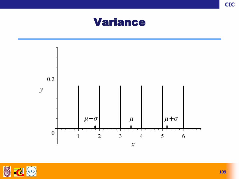
If the PMF is symmetric around a certain point,

that point must be equal to the mean.

90


CIC

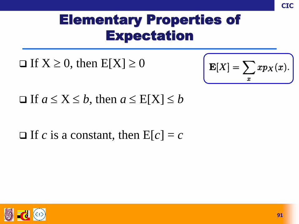
If X 0, then E[X] 0

If a X b, then a E[X] b

If c is a constant, then E[c] = c

91

Elementary Properties of

Expectation

CIC

Example 1. Let X be the number of heads in

three tosses of a fair coin. Find E[X].

92


CIC

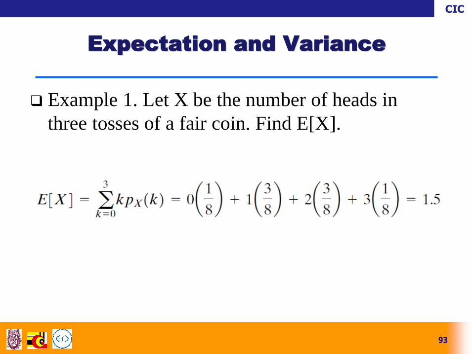
Example 1. Let X be the number of heads in

three tosses of a fair coin. Find E[X].

93


CIC

Example 2. Consider two independent coin tosses,

each with a ¾ probability of a head, and let X be the

number of heads obtained. This is a binomial r.v.

with parameters n = 2 and p = ¾. Its PMF is:

So the mean is:

94


CIC

Example 2. Consider two independent coin tosses,

each with a ¾ probability of a head, and let X be the

number of heads obtained. This is a binomial r.v.

with parameters n = 2 and p = ¾. Its PMF is:

So the mean is:

95


CIC

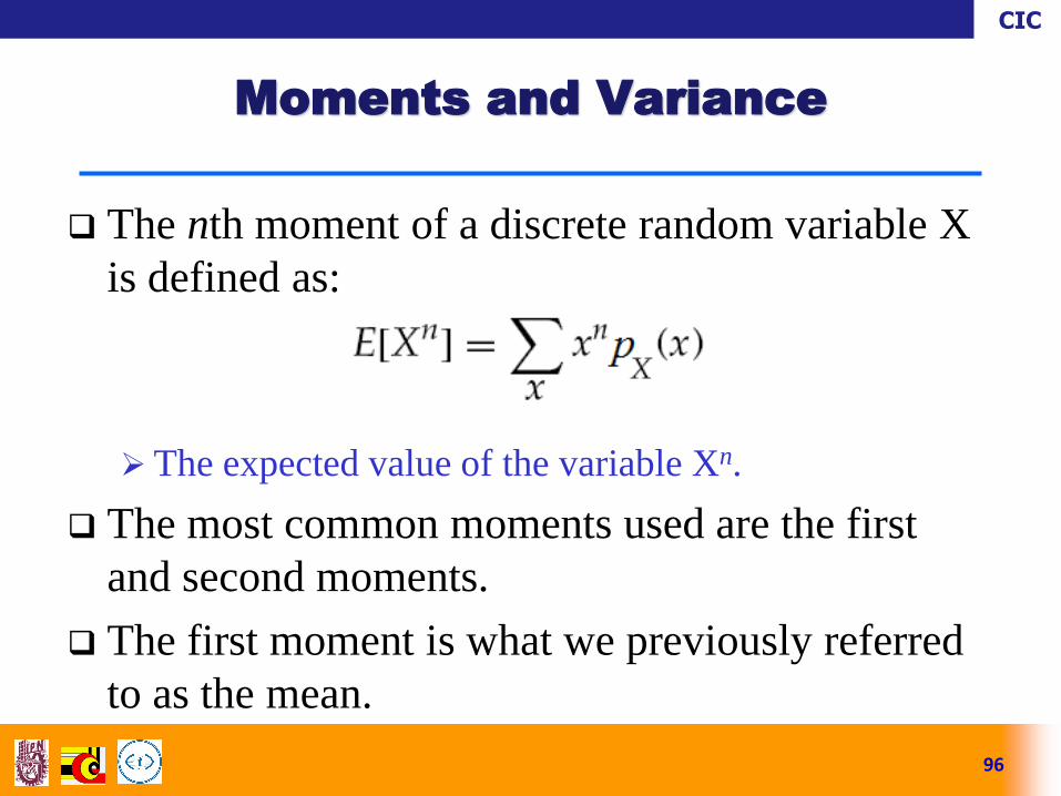
The nth moment of a discrete random variable X

is defined as:

The expected value of the variable Xn.

The most common moments used are the first

and second moments.

The first moment is what we previously referred

to as the mean.

96

Moments and Variance

CIC

The second moment of the random variable X is

the expected value of the random variable X2.

97


CIC

The central moment of the discrete random variable

X is defined as:

where μX = E[X] is the mean (first moment) of the

random variable.

The central moment of a random variable is the

moment of that random variable after its expected

value is subtracted.

98


CIC

The first central moment is always zero.

The second central moment of a discrete random

variable is its variance:

with μX = E[X].

The variance is always nonnegative.

The variance provides a measure of dispersion of

X around its mean.

99


CIC

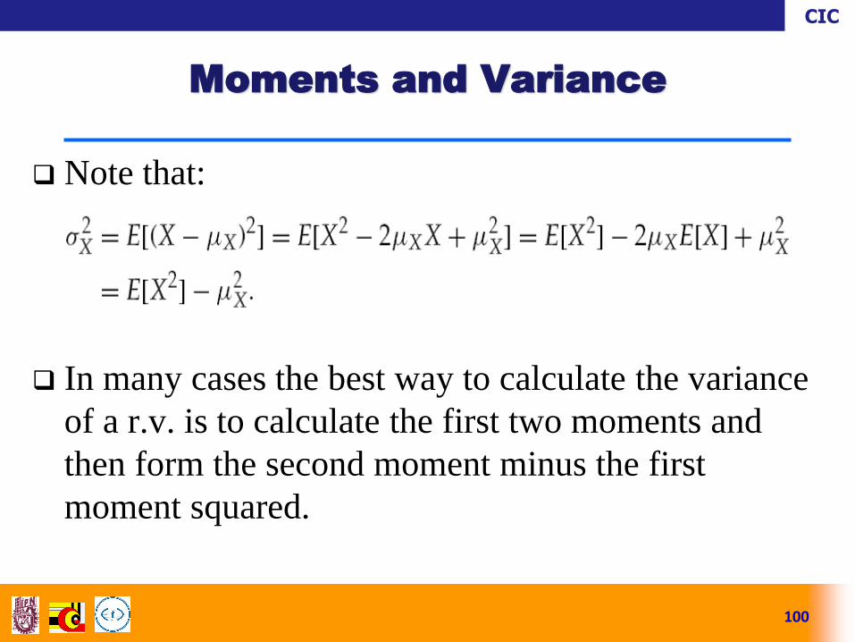
Note that:

In many cases the best way to calculate the variance

of a r.v. is to calculate the first two moments and

then form the second moment minus the first

moment squared.

100


CIC

The standard deviation is defined as the squared

root of the variance:

Both the variance and the standard deviation

serve as a measure of the width of the PDF of a

random variable.

101

Standard Deviation

CIC

Given the discrete random variable X with PMF pX ,

the expected value of a function, g(X), of that

random variable is given by:

Using this rule, the variance of X can be obtained as:

102

Expected Value Rule for Functions

of Random Variables

CIC

Example 1. Consider the random variable X,

which has PMF pX(x) given as:

The mean E[X] is equal to 0, which can be

verified by:

103

Variance

CIC

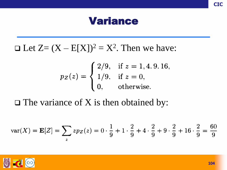
Let Z= (X – E[X])2 = X2. Then we have:

The variance of X is then obtained by:

104

Variance

CIC

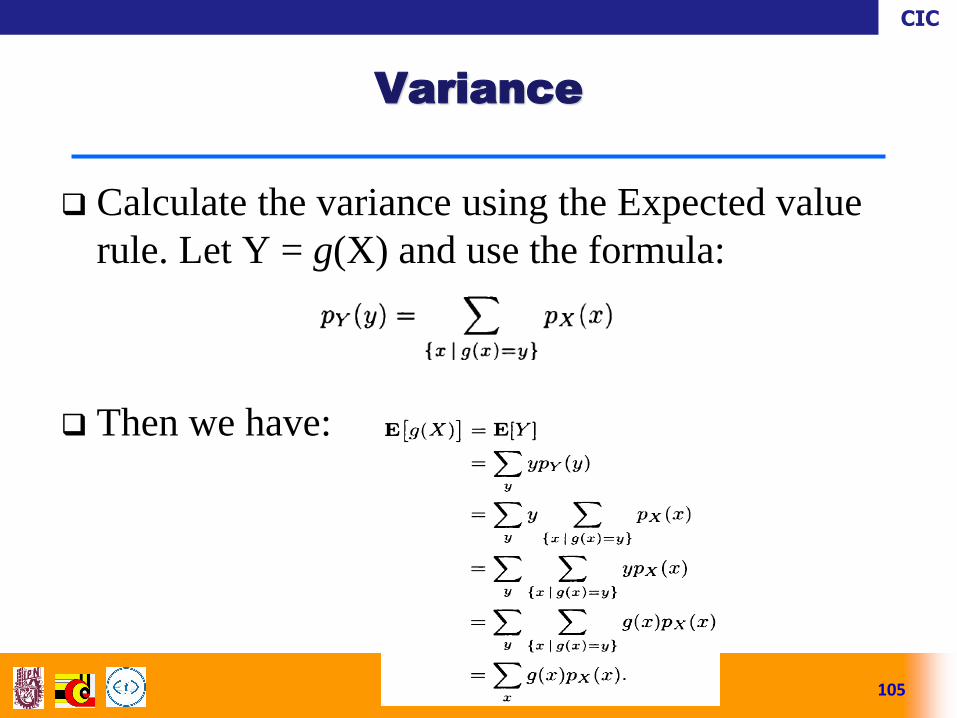
Calculate the variance using the Expected value

rule. Let Y = g(X) and use the formula:

Then we have:

105

Variance

CIC

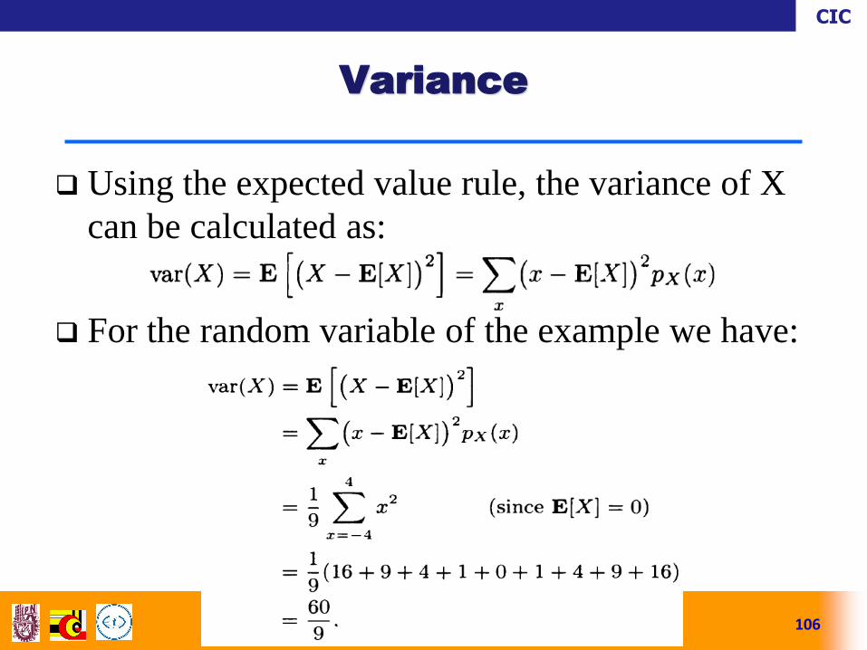
Using the expected value rule, the variance of X

can be calculated as:

For the random variable of the example we have:

106

Variance

CIC

Example 2. Roll of a Die. Let X denote the

number obtained in a roll of a die. Obtain the

mean an variance of X.

107

Variance

CIC

Example 2. Roll of a Die. Let X denote the

number obtained in a roll of a die. Obtain the

mean an variance of X.

P(X = i) = 1/6 for i = 1, 2, . . . , 6. Then μ = 3.5,

and

108

Variance

CIC

109

Variance

CIC

In some applications, we transform random variables

to a standard scale in which all random variables are

centred at 0 and have standard deviations equal to 1.

For any given r.v. X, for which μ and σ exist, we

define its standardization as the new r.v.

110

Standardization

CIC

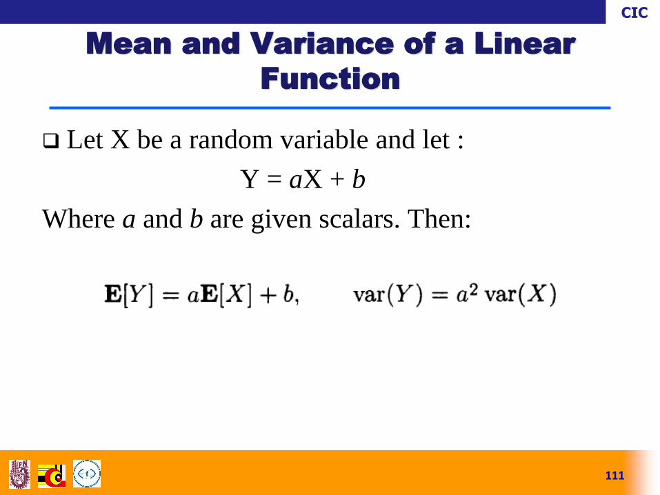
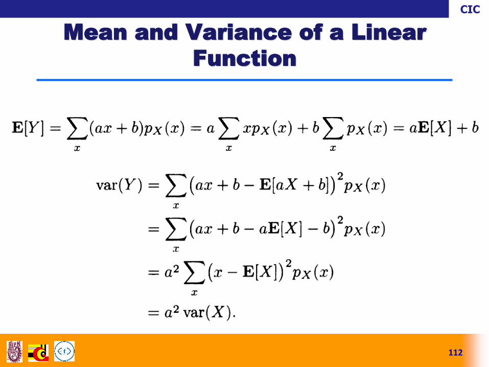
Let X be a random variable and let :

Y = aX + b

Where a and b are given scalars. Then:

111

Mean and Variance of a Linear

Function

CIC

112

Mean and Variance of a Linear

Function

CIC

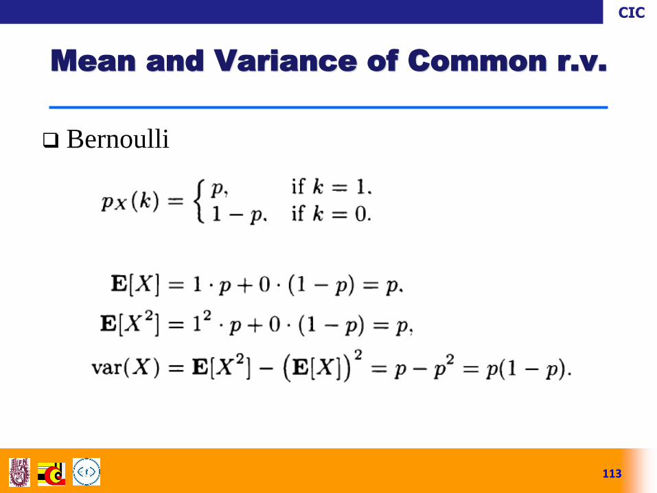
Bernoulli

113

Mean and Variance of Common r.v.

CIC

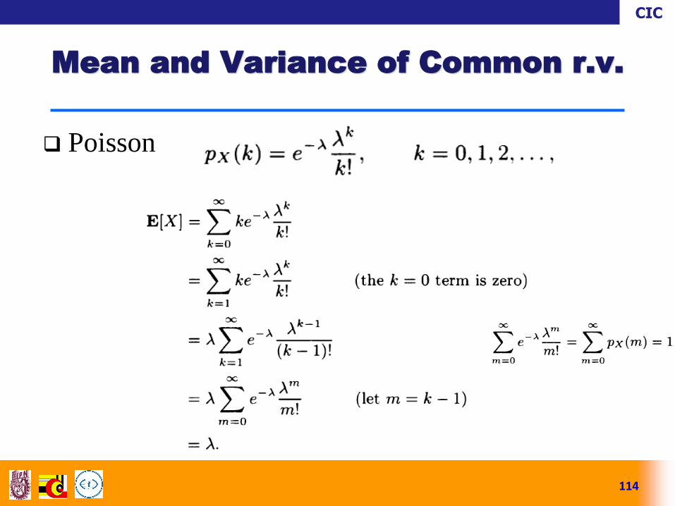
Poisson

114


CIC

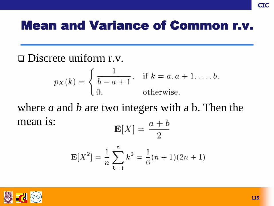
Discrete uniform r.v.

where a and b are two integers with a b. Then the

mean is:

115


CIC

We usually deal with the relationship between

multiple r.v.s in the same experiment. Medicine: To evaluate the effectiveness of a treatment, we may take

multiple measurements per patient; an ensemble of blood pressure,

heart rate, and cholesterol readings can be more informative than any

of these measurements considered separately.

Time series: To study how something evolves over time, we can often

make a series of measurements over time, and then study the series

jointly. There are many applications of such series, such as global

temperatures, stock prices, or national unemployment rates. The

series of measurements considered jointly can help us deduce trends

for the purpose of forecasting future measurements.

116

Joint PMFS of Multiple Random

Variables

CIC

Consider two discrete random variables X and Y

associated with the same experiment.

The probabilities of the values that X and Y can take

are captured by joint PMF of X and Y, denoted pX,Y .

If (x,y) is a pair of possible values of X and Y, the

joint PMF of X and Y is the function pX,Y given by:

The joint PMF of n r.v.s is defined analogously.

117


Variables

CIC

118


Variables

CIC

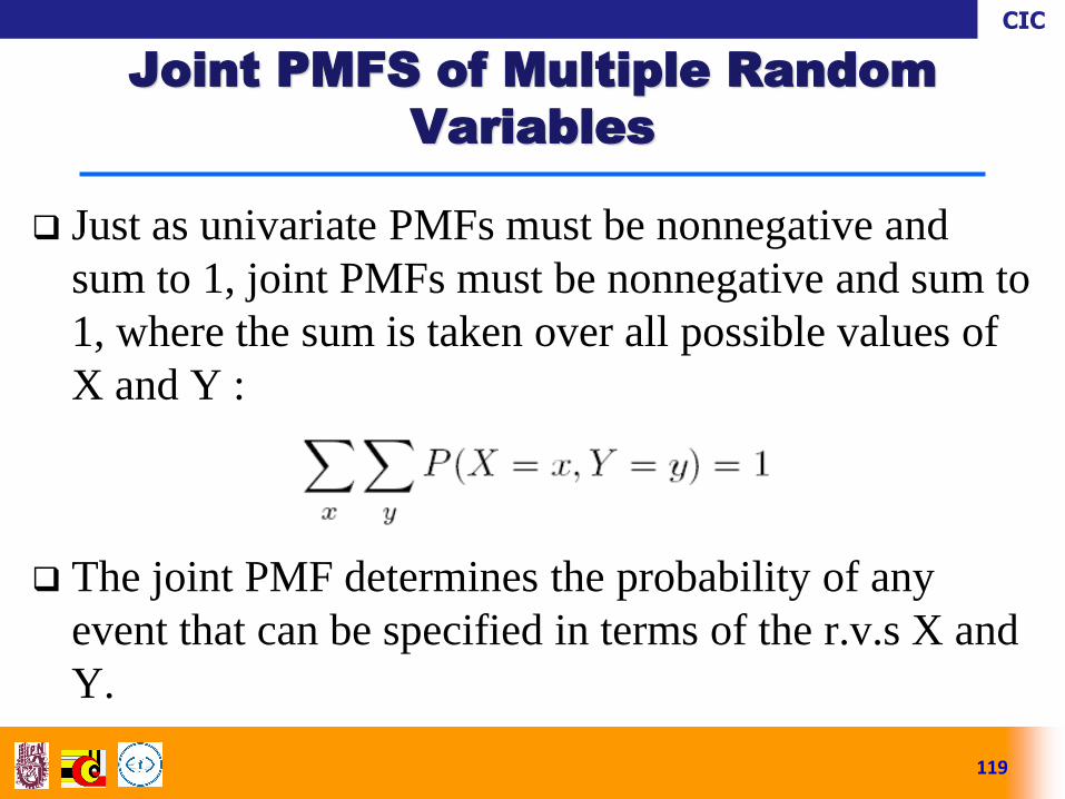
Just as univariate PMFs must be nonnegative and

sum to 1, joint PMFs must be nonnegative and sum to

1, where the sum is taken over all possible values of

X and Y :

The joint PMF determines the probability of any

event that can be specified in terms of the r.v.s X and

Y.

119


Variables

CIC

In terms of their joint sample space:

120


Variables

CIC

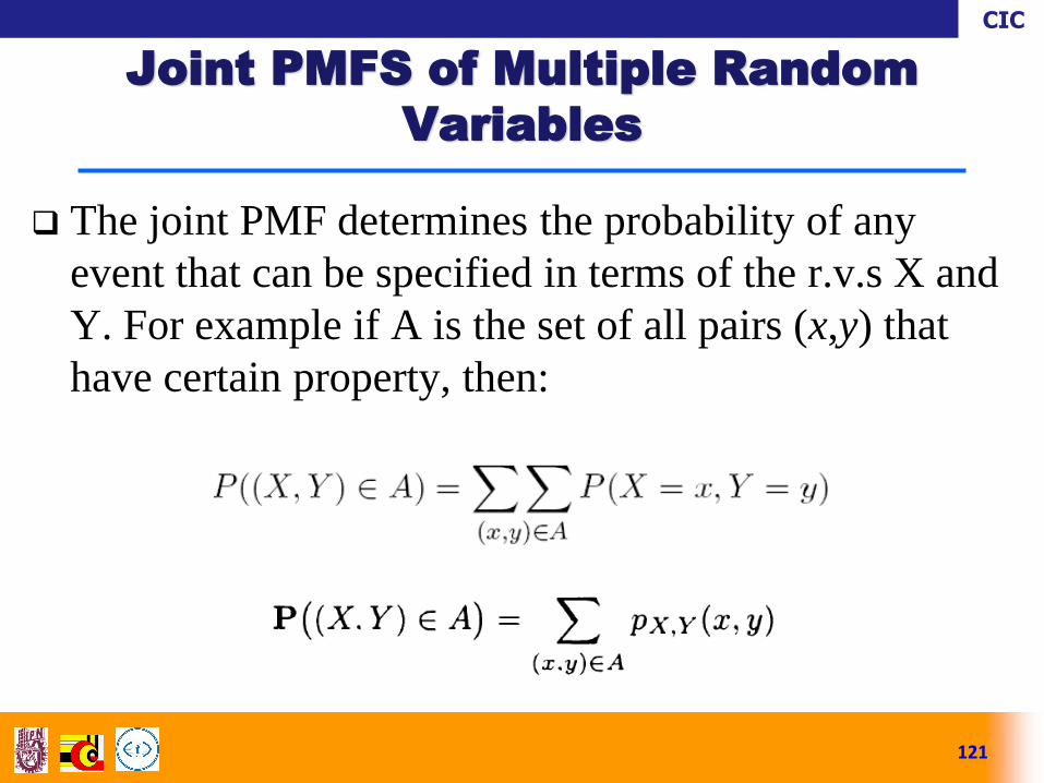
The joint PMF determines the probability of any

event that can be specified in terms of the r.v.s X and

Y. For example if A is the set of all pairs (x,y) that

have certain property, then:

121


Variables

CIC

From the joint distribution of X and Y, the PMF of X

alone can be obtained by summing over the possible

values of Y. The same apply for the case of obtaining

the PMF of Y:

122


Variables

CIC

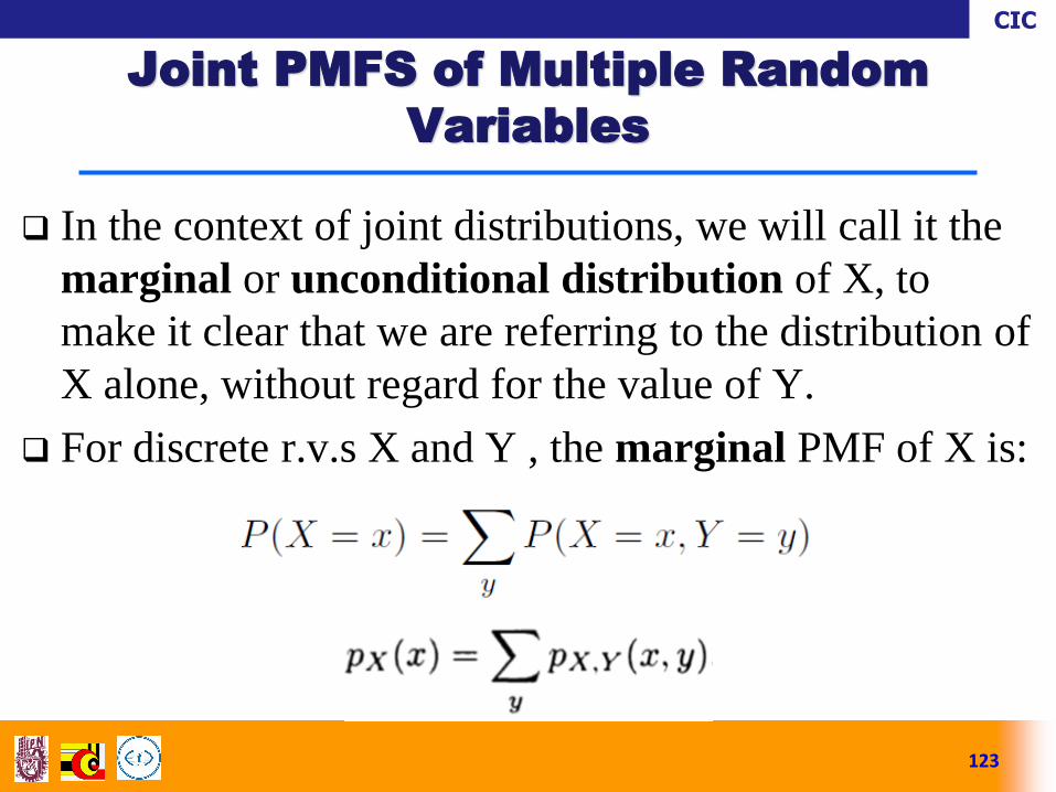
In the context of joint distributions, we will call it the

marginal or unconditional distribution of X, to

make it clear that we are referring to the distribution of

X alone, without regard for the value of Y.

For discrete r.v.s X and Y , the marginal PMF of X is:

123


Variables

CIC

The operation of summing over

the possible values of Y in

order to convert the joint PMF

into the marginal PMF of X is

known as marginalizing out Y.

.

The marginal PMF of X is the

PMF of X, viewing X

individually rather than jointly

with Y.

124


Variables

CIC

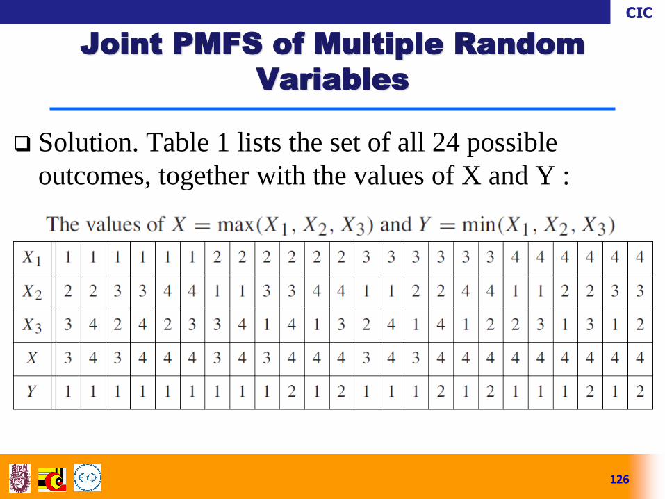
Example 1. Maximum and Minimum of Three

Integers. Choose three numbers X1, X2, X3 without

replacement and with equal probabilities from the set

{1, 2, 3, 4}, and let X = max{X1, X2, X3} and Y =

min{X1, X2, X3}. Find the joint PMF of X and Y .

125


Variables

CIC

Solution. Table 1 lists the set of all 24 possible

outcomes, together with the values of X and Y :

126


Variables

CIC

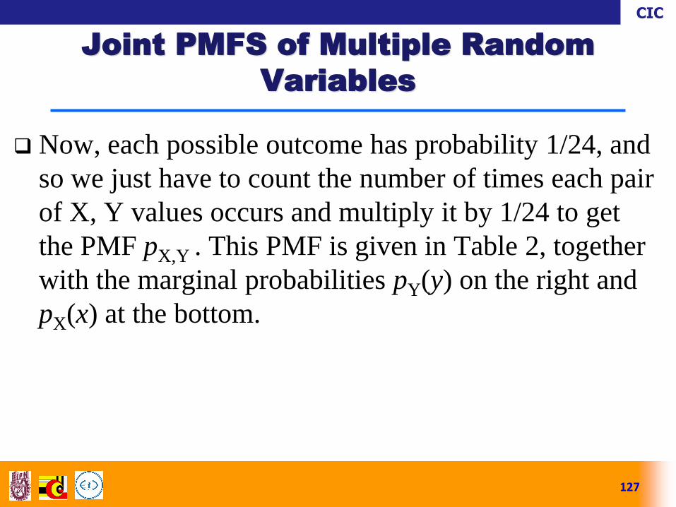
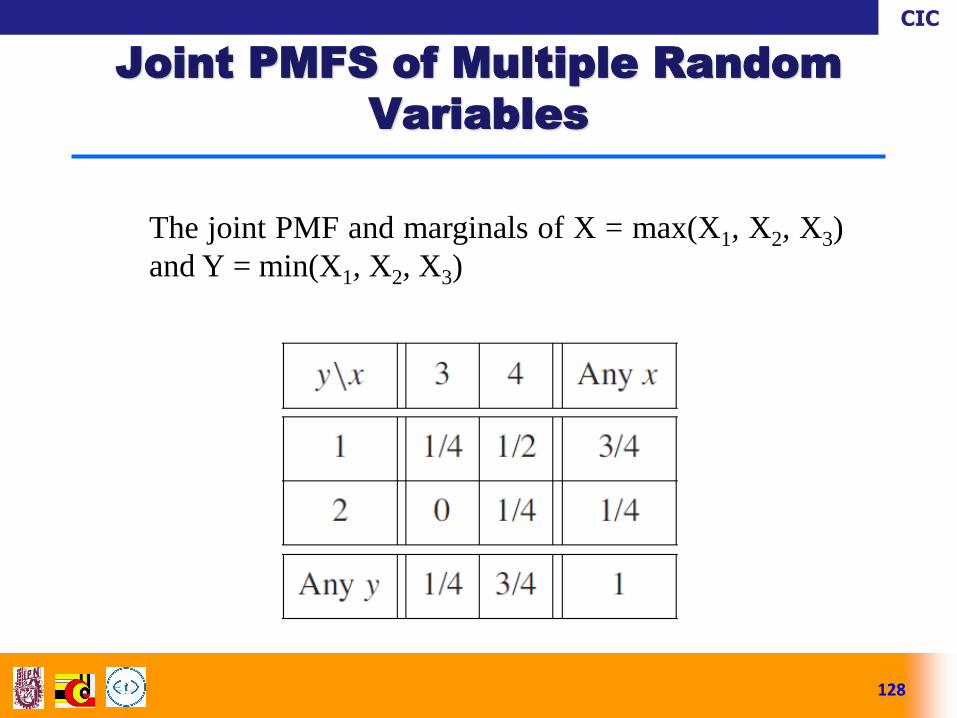
Now, each possible outcome has probability 1/24, and

so we just have to count the number of times each pair

of X, Y values occurs and multiply it by 1/24 to get

the PMF pX,Y . This PMF is given in Table 2, together

with the marginal probabilities pY(y) on the right and

pX(x) at the bottom.

127


Variables

CIC

128


Variables

The joint PMF and marginals of X = max(X1, X2, X3)

and Y = min(X1, X2, X3)

CIC

A function Z = ɡ(X,Y) of the random variables X

and Y defines another random variable. Its PMF

can be calculated from the joint PMF pX,Y

according to:

129

Functions of Multiple Random

Variables

CIC

The expected value rule applies and takes the

form:

In the case where ɡ is linear and of the form

aX+bY+c, where a, b, c are given scalars:

130

Functions of Multiple Random

Variables

CIC

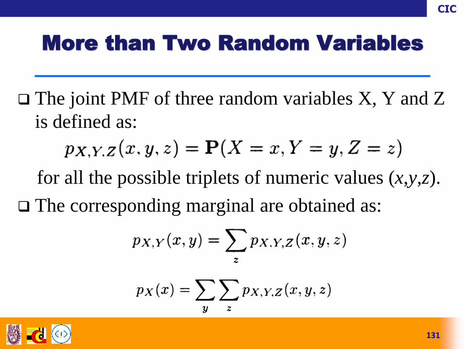
The joint PMF of three random variables X, Y and Z

is defined as:

for all the possible triplets of numeric values (x,y,z).

The corresponding marginal are obtained as:

131

More than Two Random Variables

CIC

The expected value rule for functions is given by:

If ɡ is linear and has the form aX+bY+cZ+d, then:

132

More than Two Random Variables

CIC

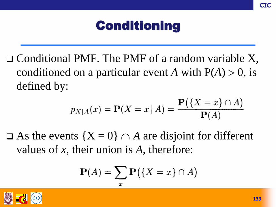
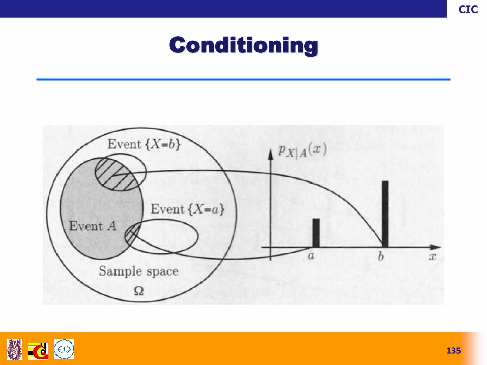
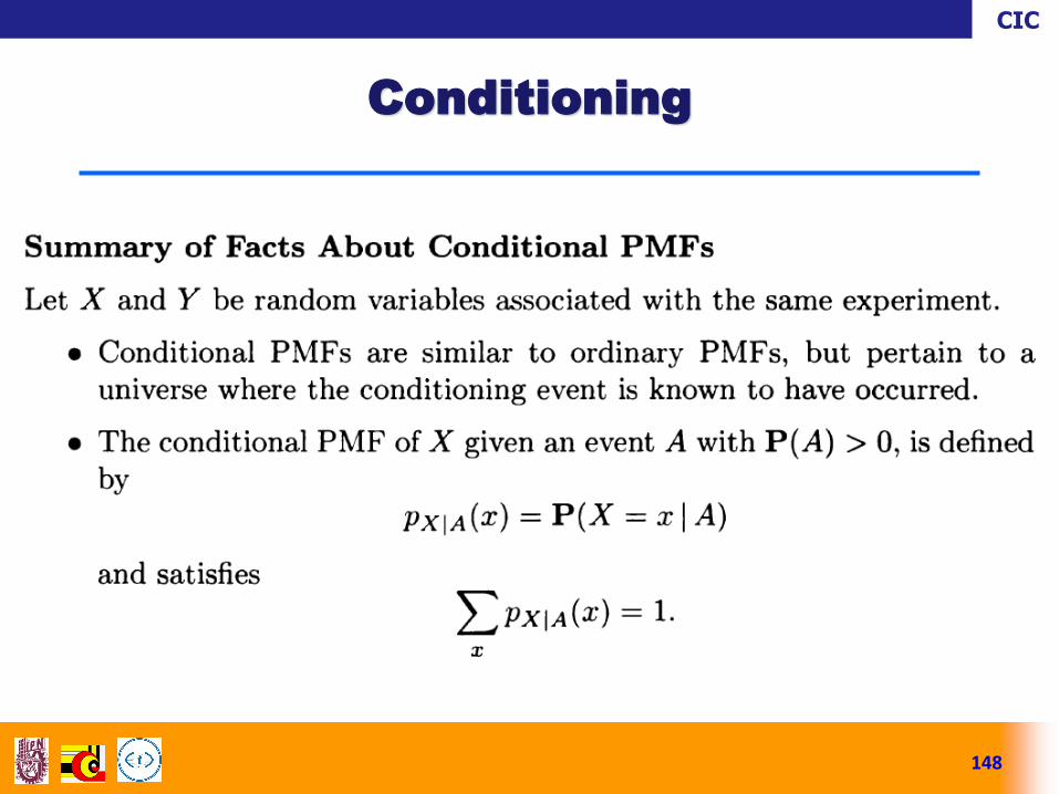
Conditional PMF. The PMF of a random variable X,

conditioned on a particular event A with P(A) 0, is

defined by:

As the events {X = 0} A are disjoint for different

values of x, their union is A, therefore:

133

Conditioning

CIC

Combining the previous two formulas:

so pX|A is a legitimate PMF.

The conditional PMF is calculated similar to its

unconditional counterpart: to obtain pX|A we add the

probabilities of the outcomes that give rise to X = x

and belong to the conditioning event A, and then

normalise by dividing with P(A).

134

Conditioning

CIC

135

Conditioning

CIC

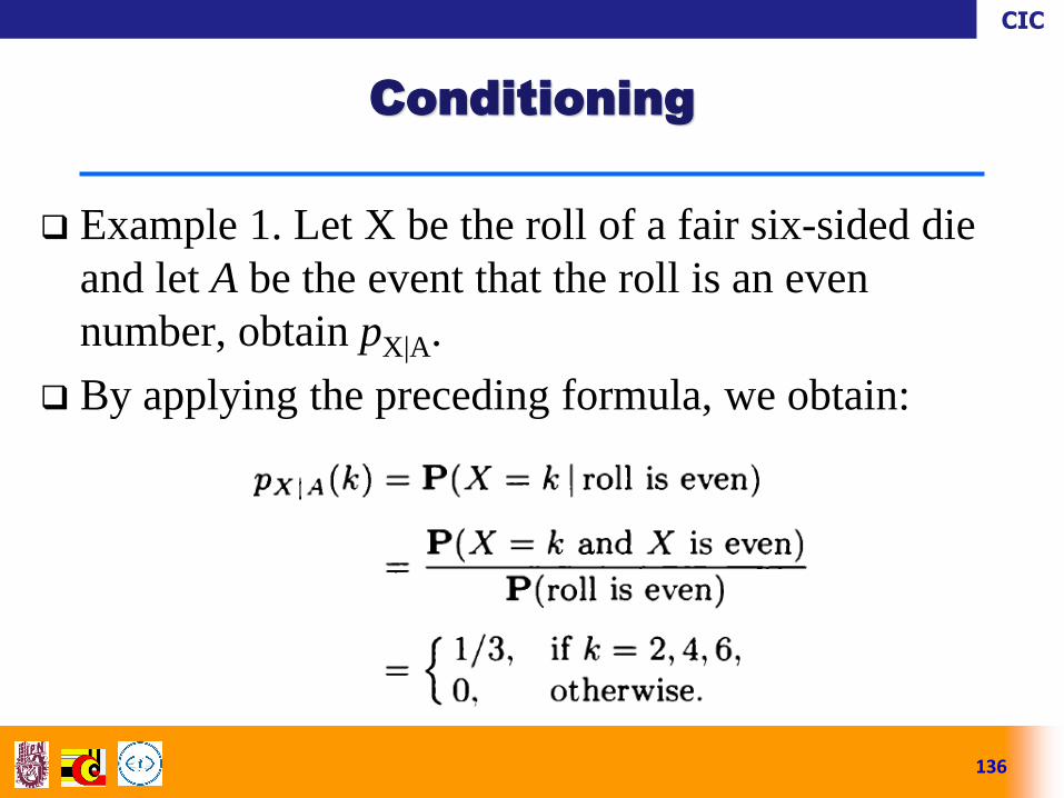
Example 1. Let X be the roll of a fair six-sided die

and let A be the event that the roll is an even

number, obtain pX|A.

By applying the preceding formula, we obtain:

136

Conditioning

CIC

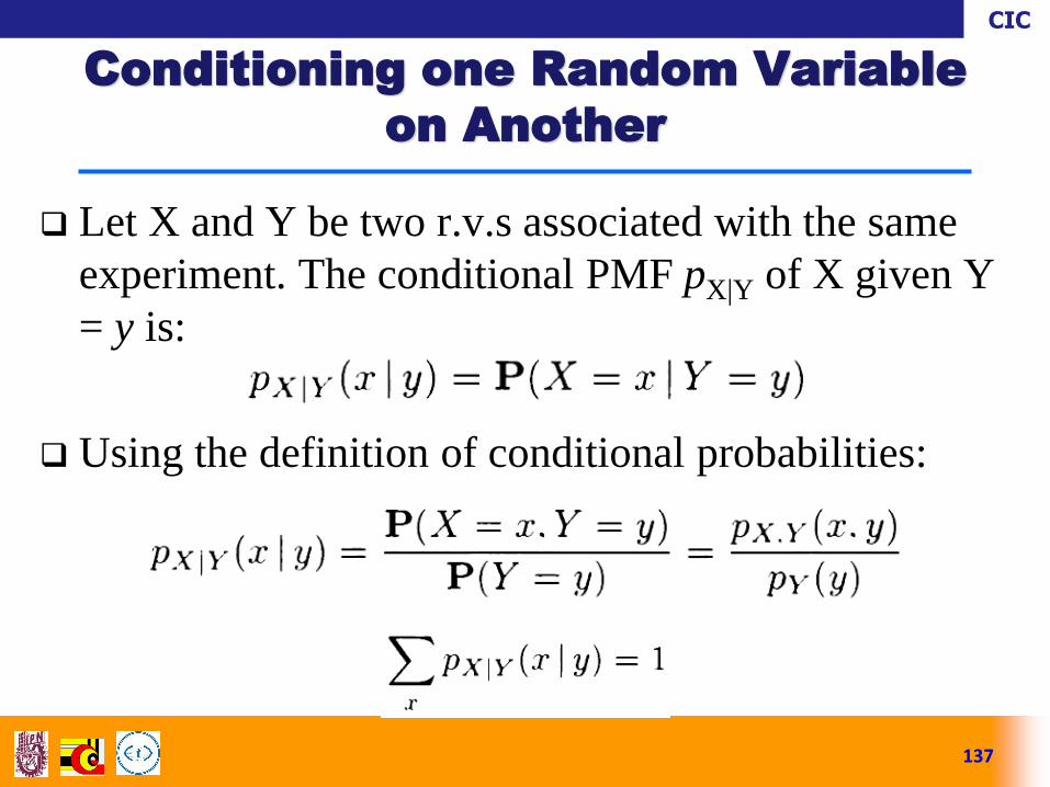
Let X and Y be two r.v.s associated with the same

experiment. The conditional PMF pX|Y of X given Y

= y is:

Using the definition of conditional probabilities:

137

Conditioning one Random Variable

on Another

CIC

138

Conditioning one Random Variable

on Another

CIC

The conditional PMF is often convenient for the

calculation of the joint PMF, using a sequential

approach and the formula:

Or its counterpart:

139

Conditioning

CIC

140

Conditioning

CIC

141

Conditioning

CIC

142

Conditioning

CIC

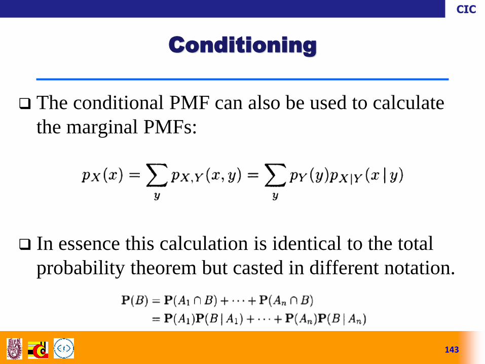
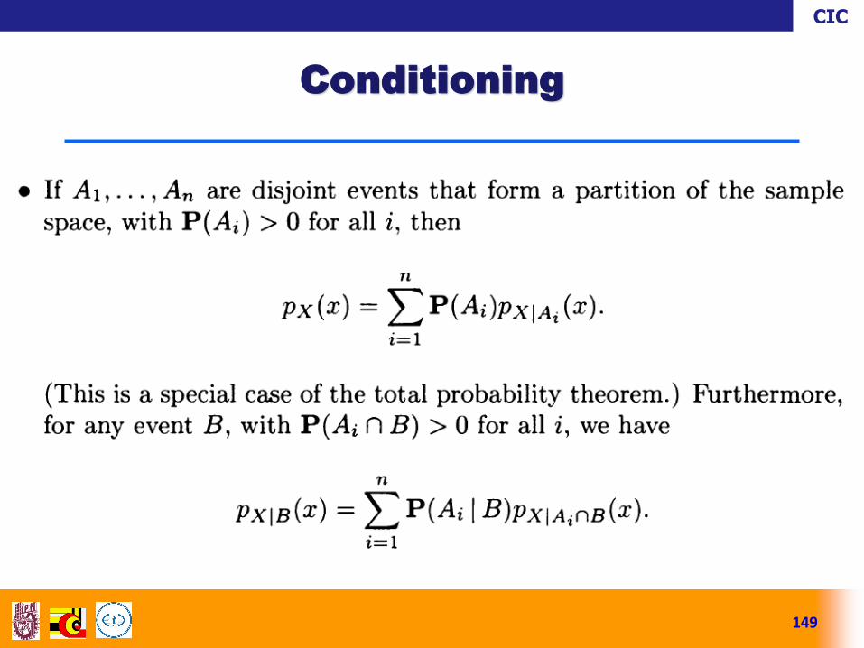
The conditional PMF can also be used to calculate

the marginal PMFs:

In essence this calculation is identical to the total

probability theorem but casted in different notation.

143

Conditioning

CIC

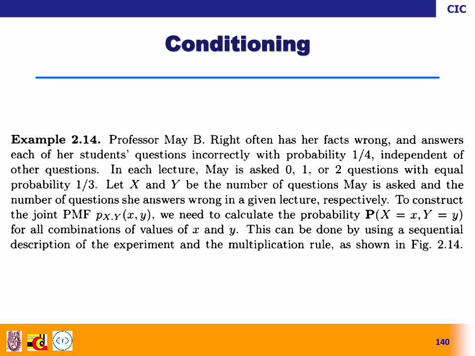
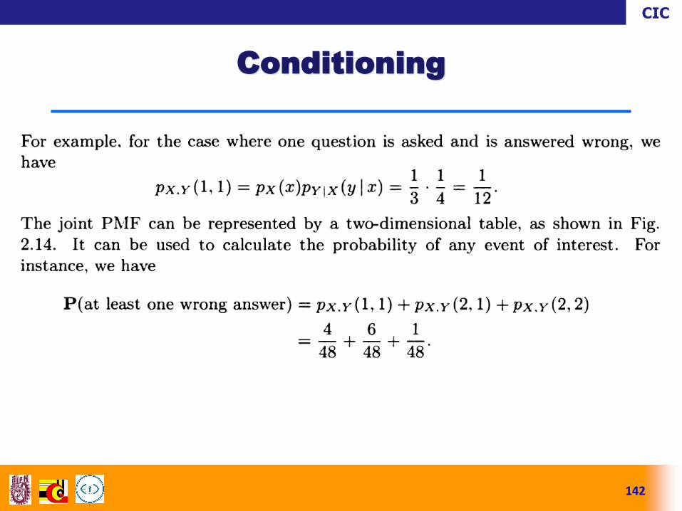
Example 3. Consider a transmitter that is sending

messages over a computer network. Let us define the

following two random variables:

X: the travel time of a given message,

Y: the length of the given message

Knowing the PMF of the travel time of a message

that has a given length, and the PMF of the message

length, find the (unconditional) PMF of the travel of

a message.

144

Conditioning

CIC

Solution. Assuming that the length of the message

can take two possible values:

y =102 bytes with probability 5/6

y = 104 bytes with probability 1/6

Assume that the travel time X of the message

depends on its length Y and the congestion in the

network at the time of transmission.

145

Conditioning

CIC

In particular, the travel time is 10-4Y seconds with

probability 1/2, 10-3Y seconds with probability 1/3,

and 10-2Y seconds with probability 1/6. Thus:

146

Conditioning

CIC

To find the PMF of X, use the total probability

formula:

Therefore:

147

Conditioning

CIC

148

Conditioning

CIC

149

Conditioning

CIC

150

Conditioning

CIC

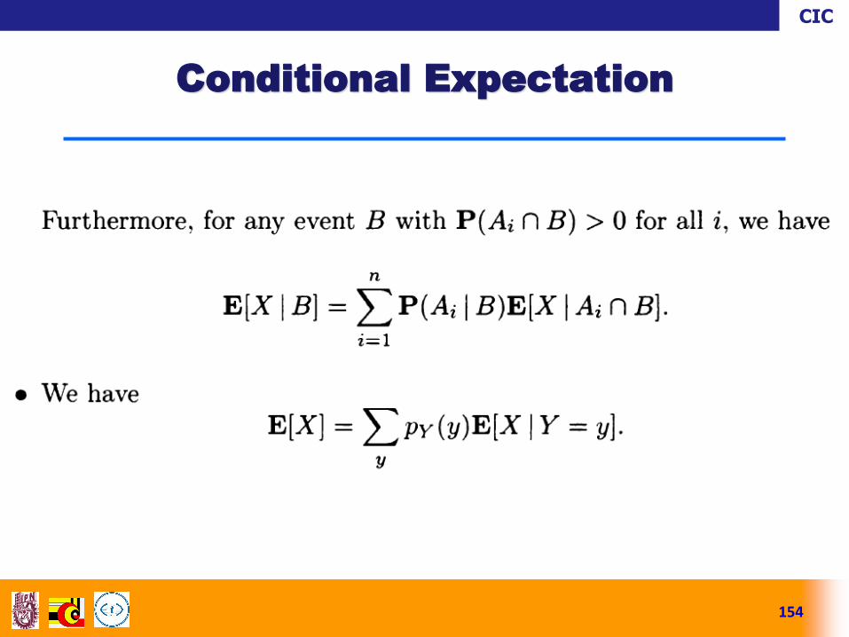
A conditional expectation is the same as an ordinary

expectation, except that it refers to the new universe.

All probabilities and PMFs are replaced by their

conditional counterparts.

Conditional variance can also be treated similarly.

151

Conditional Expectation

CIC

152


CIC

153


CIC

154


CIC

155


CIC

156


Example 4. Messages transmitted by a computer in Boston

through a data network are destined for New York with

probability 0.5, for Chicago with probability 0.3, and for San

Francisco with probability 0.2. The transit time X of a message is

random. Its mean is 0.05 seconds if it is destined for New York,

0.1 seconds if it is destined for Chicago, and 0.3 seconds if it is

destined for San Francisco. Then, E[X] is easily calculated using

the total expectation theorem as

CIC

The independence of a random variable from an

event is similar to the independence of two events.

Knowing the occurrence of the conditioning event provides

no new information on the value of the random variable.

Formally, the random variable X is independent of

the event A if:

so that as long as P(A) 0, independence is the same as

the conditioning:

157

Independence of a Random

Variable from an Event

CIC

158

Independence

CIC

159

Independence

CIC

Two random variables X and Y are independent if:

This is the same as requiring that the two events {X =

x} and {Y = y} be independent for every x and y.

The formula shows that

independence is equivalent to the condition:

This means that the value of Y provides no

information on the value of X.

160

Independence of Random Variables

CIC

There is a similar notion of conditional independence

of two random variables, given an even A wit P(A) > 0.

Let X and Y said to be conditional independent,

given a positive probability event A, if:

161


CIC

162


CIC

In a similar calculation it can be shown that if X and

Y are independent, then:

for any functions ɡ and h.

This follows immediately once we realise that if X

and Y are independent, then the same is true for ɡ(x) and h(y).

163


CIC

Consider now the sum X + Y of two independent

random variables and let calculate its variance.

Considering zero-mean random variables

and , then we have:

164


The variance of the sum of two

independent random variables

is equal to the sum of their

variances

CIC

165


CIC

166


CIC

167

Independence of Several Random

Variables

Three random variables X, Y, and Z are said to be

independent if:

If X, Y, and Z are independent random variables,

then any three random variables f(X), g(Y), and h(Z),

are also independent.

The random variables of the form g(X,Y) and h(Y,Z)

are usually not independent because they are both

affected by Y.

CIC

168

Variance of the Sum of Independent

Random Variables

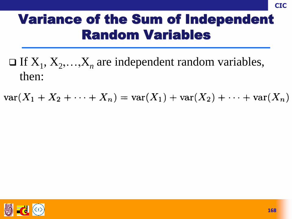
If X1, X2,…,Xn are independent random variables,

then:

CIC

169


Random Variables

CIC

170


Random Variables

CIC

171


Random Variables

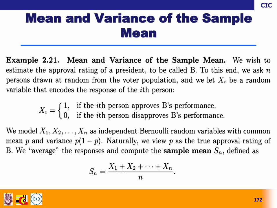
The formulas for the mean and variance of a

weighted sum of random variables form the basis for

many statistical procedures that estimate the mean of

a random variable by averaging many independent

samples.

CIC

172

Mean and Variance of the Sample

Mean

CIC

173


Mean

CIC

174


Mean

CIC

175

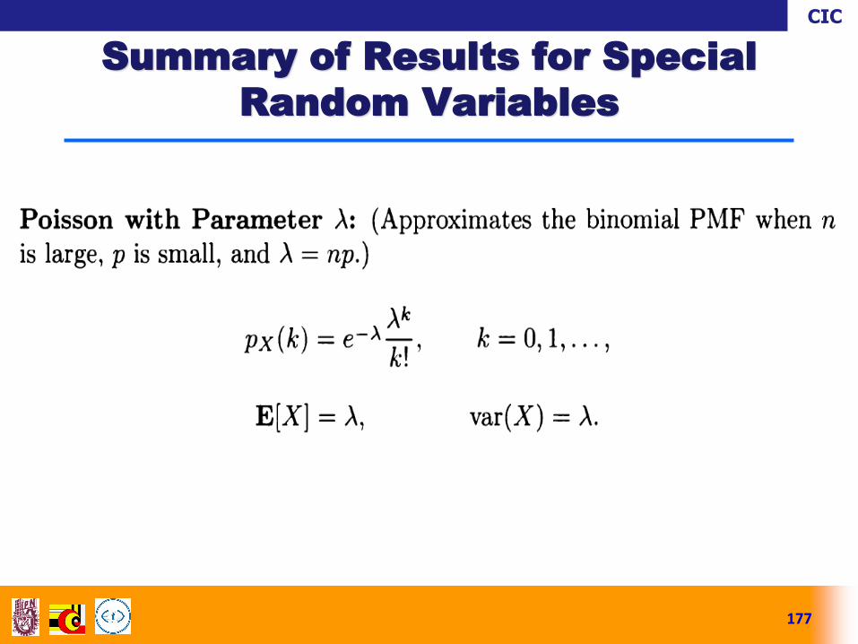
Summary of Results for Special

Random Variables

CIC

176


Random Variables

CIC

177


Random Variables

probability, random processes and inference - cic …pescamilla/prpi/slides/prpi_2.pdf ·...

Documents