probability, random processes and inference - cic …pescamilla/prpi/slides/prpi_5.pdf ·...
TRANSCRIPT
INSTITUTO POLITÉCNICO NACIONAL CENTRO DE INVESTIGACION EN COMPUTACION
Probability, Random Processes and Inference
Dr. Ponciano Jorge Escamilla Ambrosio [email protected]
http://www.cic.ipn.mx/~pescamilla/
Laboratorio de
Ciberseguridad
CIC
2
Course Content
2. Introduction to Random Processes
2.1. Markov Chains
2.1.1. Discrete Time Markov Chains
2.1.2. Classification of States
2.1.3. Steady State Behavior
2.1.4. Absorption Probabilities and Expected Time to
Absorption
2.1.5. Continuous Time Markov Chains
2.1.6. Ergodic Theorem for Discrete Markov Chains
2.1.7. Markov Chain Montecarlo Method
2.1.8. Queuing Theory
CIC
A random or stochastic process is a mathematical
model for a phenomenon that evolves in time in an
unpredictable manner from the viewpoint of the
observer.
It may be unpredictable because of such effects as
interference or noise in a communication link or
storage medium, or it may be an information-bearing
signal, deterministic from the viewpoint of an
observer at the transmitter but random to an observer
at the receiver.
3
Stochastic (Random) Processes
CIC
A stochastic (or random) process is a mathematical
model of a probabilistic experiment that evolves in
time and generates a sequence of numerical values.
A stochastic process can be used to model:
The sequence of daily prices of a stock;
The sequence of scores in a football game;
The sequence of failure times of a machine;
The sequence of hourly traffic loads at a node of a communication
network;
The sequence of radar measurements of the position of an airplane.
4
Stochastic (Random) Processes
CIC
Each numerical value in the sequence is modelled by
a random variable.
A stochastic process is simply a (finite or infinite)
sequence of random variables.
We are still dealing with a single basic experiment
that involves outcomes governed by a probability
law, and random variables that inherit their
probabilistic properties from that law.
5
Stochastic (Random) Processes
CIC
Stochastic processes involve some changes with respect to
earlier models:
Tend to focus on the dependencies in the sequence of values
generated by the process.
o How do future prices of a stock depend on past values?
Are often interested in long-term averages involving the entire
sequence of generated values.
o What is the fraction of time that a machine is idle?
Wish to characterize the likelihood or frequency of certain
boundary events.
o What is the probability that within a given hour all circuits of some
telephone system become simultaneously busy?
6
Stochastic (Random) Processes

CIC
There is a wide variety of stochastic processes.
Two major categories are of concern of this course:
Arrival-Type Processes. The occurrences have the character
of an “arrival”, such as message receptions at a receiver, job
completions in a manufacturing cell, etc. These are models in
which the interarrival times (the times between successive
arrivals) are independent random variables.
oBernoulli process. Arrivals occur in discrete times and the
interarrival times are geometrically distributed.
oPoisson process. Arrivals occur in continuous time and the
interarrivals times are exponentially distributed.
7
Stochastic (Random) Processes

CIC
Two major categories are of concern of this course:
Markov Processes. Involve experiments that evolve in
time and which the future evolution exhibits a
probabilistic dependence on the past. As an example, the
future daily prices of a stock are typically dependent on
past prices.
o In a Markov process, it is assumed a very special type of
dependence: the next value depends on past values only
through the current value.
8
Stochastic (Random) Processes
CIC
Markov chains were first introduced in 1906 by
Andrey Markov (of Markov’s inequality), with the
goal of showing that the law of large numbers can
apply to random variables that are not independent.
Markov began the study of an important new type of
chance process. In this process, the outcome of a
given experiment can affect the outcome of the next
experiment. This type of process is called a Markov
chain.
9
Discrete-Time Markov Chains

CIC
Since their invention, Markov chains have become
extremely important in a huge number of fields such
as biology, game theory, finance, machine learning,
and statistical physics.
They are also very widely used for simulations of
complex distributions, via algorithms known as
Markov chain Monte Carlo (MCMC).
10
Discrete-Time Markov Chains
CIC
Markov chains “live” in both space and time: the set
of possible values of the Xn is called the state space,
and the index n represents the evolution of the
process over time.
The state space of a Markov chain can be either
discrete or continuous, and time can also be either
discrete or continuous.
in the continuous-time setting, we would imagine a
process Xt defined for all real t 0.
11
Discrete-Time Markov Chains
CIC
Consider first discrete-time Markov chains, in which
the state changes at certain discrete time instants,
indexed by an integer variable n.
At each time step n, the state of the chain is denoted
by Xn and belongs to a finite set S of possible states,
called state space.
Specifically, we will assume that S = {1, 2,…, m},
for some positive integer m.
12
Discrete-Time Markov Chains
CIC
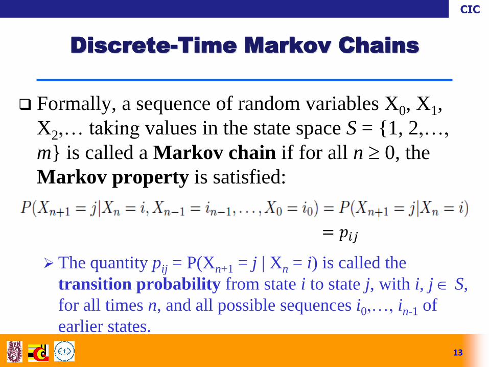
Formally, a sequence of random variables X0, X1,
X2,… taking values in the state space S = {1, 2,…,
m} is called a Markov chain if for all n 0, the
Markov property is satisfied:
The quantity pij = P(Xn+1 = j | Xn = i) is called the
transition probability from state i to state j, with i, j S,
for all times n, and all possible sequences i0,…, in-1 of
earlier states.
13
Discrete-Time Markov Chains
= 𝑝𝑖𝑗
CIC
Whenever the state happens to be i, there is
probability pij that the next state is equal to j.
The key assumption underlying the Markov chains is
that the transition probabilities pij apply whenever
state i is visited, no matter what happened in the
past, and no matter how state i was reached.
The probability law of the next state Xn+1 depends
on the past only through the value of the present
state Xn.
14
Discrete-Time Markov Chains
CIC
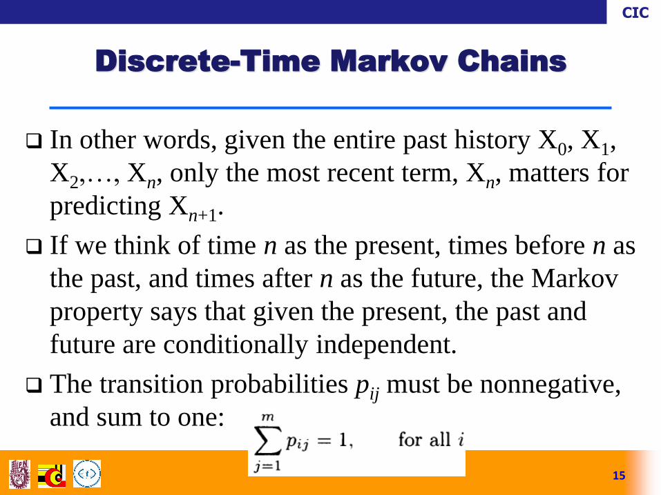
In other words, given the entire past history X0, X1,
X2,…, Xn, only the most recent term, Xn, matters for
predicting Xn+1.
If we think of time n as the present, times before n as
the past, and times after n as the future, the Markov
property says that given the present, the past and
future are conditionally independent.
The transition probabilities pij must be nonnegative,
and sum to one:
15
Discrete-Time Markov Chains

CIC
16
Discrete-Time Markov Chains
CIC
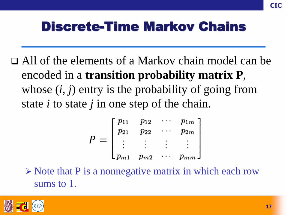
All of the elements of a Markov chain model can be
encoded in a transition probability matrix P,
whose (i, j) entry is the probability of going from
state i to state j in one step of the chain.
Note that P is a nonnegative matrix in which each row
sums to 1.
17
Discrete-Time Markov Chains
𝑃 =
CIC
It is also helpful to lay out the model in the so-called
transition probability graph, whose nodes are the
states and whose arcs are the possible transitions.
By recording the numerical values of pij near the
corresponding arcs, one can visualize the entire
model in a way that can make some of its major
properties readily apparent.
18
Discrete-Time Markov Chains

CIC
Example 1. Rainy-sunny Markov chain. Suppose that on any
given day, the weather can either be rainy or sunny. If today
is rainy, then tomorrow will be rainy with probability 1/3
and sunny with probability 2/3. If today is sunny, then
tomorrow will be rainy with probability 1/2 and sunny with
probability 1/2. Letting Xn be the weather on day n,
X0,X1,X2, . . . is a Markov chain on the state space {R, S},
where R stands for rainy and S for sunny. We know that the
Markov property is satisfied because, from the description of
the process, only today’s weather matters for predicting
tomorrow’s.
19
Discrete-Time Markov Chains

CIC
Transition probability matrix:
Transition probability graph:
20
Discrete-Time Markov Chains
CIC
Example 2. According to Kemeny, Snell, and
Thompson, the Land of Oz is blessed by many
things, but not by good weather. They never have
two nice days in a row. If they have a nice day, they
are just as likely to have snow as rain the next day. If
they have snow or rain, they have an even chance of
having the same the next day. If there is change from
snow or rain, only half of the time is this a change to
a nice day. With this information, form a Markov
chain model.
21
Discrete-Time Markov Chains
CIC
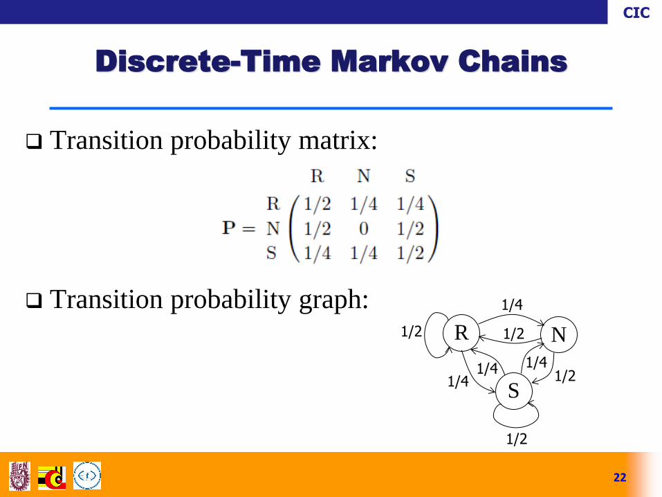
Transition probability matrix:
Transition probability graph:
22
Discrete-Time Markov Chains
R N
S
1/2
1/2
1/4
1/2
1/4 1/4 1/2
1/4
CIC
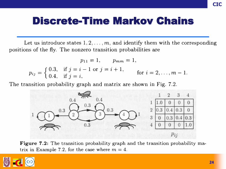
Example 3. Spiders and Fly. A fly moves along a
straight line in unit increments. At each time period,
it moves one unit to the left with probability 0.3, one
unit to the right with probability 0.3, and stays in
place with probability 0.4, independent of the past
history of movements. Two spiders are lurking at
positions 1 and m; if the fly lands there, it is
captured by a spider, and the process terminates.
Construct a Markov chain model, assuming that the
fly starts in a position between 1 and m.
23
Discrete-Time Markov Chains
CIC
24
Discrete-Time Markov Chains
CIC
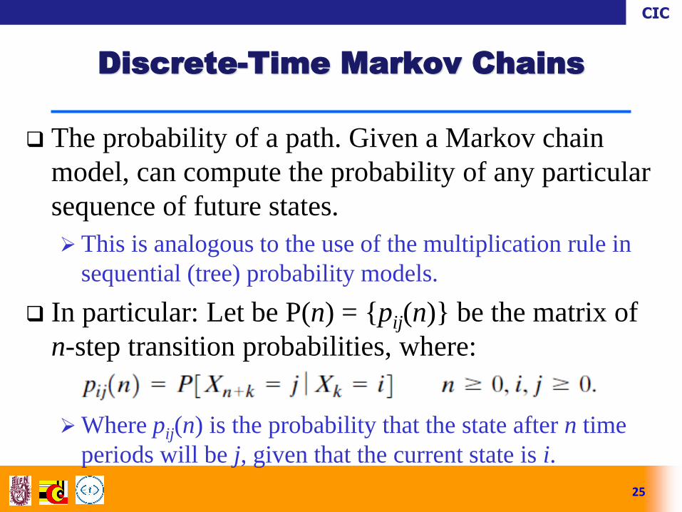
The probability of a path. Given a Markov chain
model, can compute the probability of any particular
sequence of future states.
This is analogous to the use of the multiplication rule in
sequential (tree) probability models.
In particular: Let be P(n) = {pij(n)} be the matrix of
n-step transition probabilities, where:
Where pij(n) is the probability that the state after n time
periods will be j, given that the current state is i.
25
Discrete-Time Markov Chains
CIC
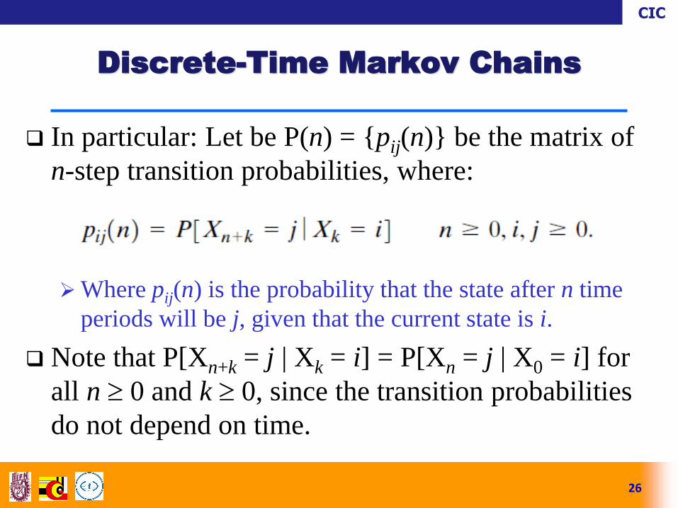
In particular: Let be P(n) = {pij(n)} be the matrix of
n-step transition probabilities, where:
Where pij(n) is the probability that the state after n time
periods will be j, given that the current state is i.
Note that P[Xn+k = j | Xk = i] = P[Xn = j | X0 = i] for
all n 0 and k 0, since the transition probabilities
do not depend on time.
26
Discrete-Time Markov Chains

CIC
First, consider the two-step transition probabilities.
The probability of going from state i at t = 0 passing
through state k at t = 1, and ending at state j at t = 2
is:
27
Discrete-Time Markov Chains
CIC
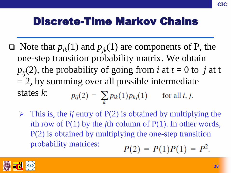
Note that pik(1) and pjk(1) are components of P, the
one-step transition probability matrix. We obtain
pij(2), the probability of going from i at t = 0 to j at t
= 2, by summing over all possible intermediate
states k:
This is, the ij entry of P(2) is obtained by multiplying the
ith row of P(1) by the jth column of P(1). In other words,
P(2) is obtained by multiplying the one-step transition
probability matrices:
28
Discrete-Time Markov Chains
CIC
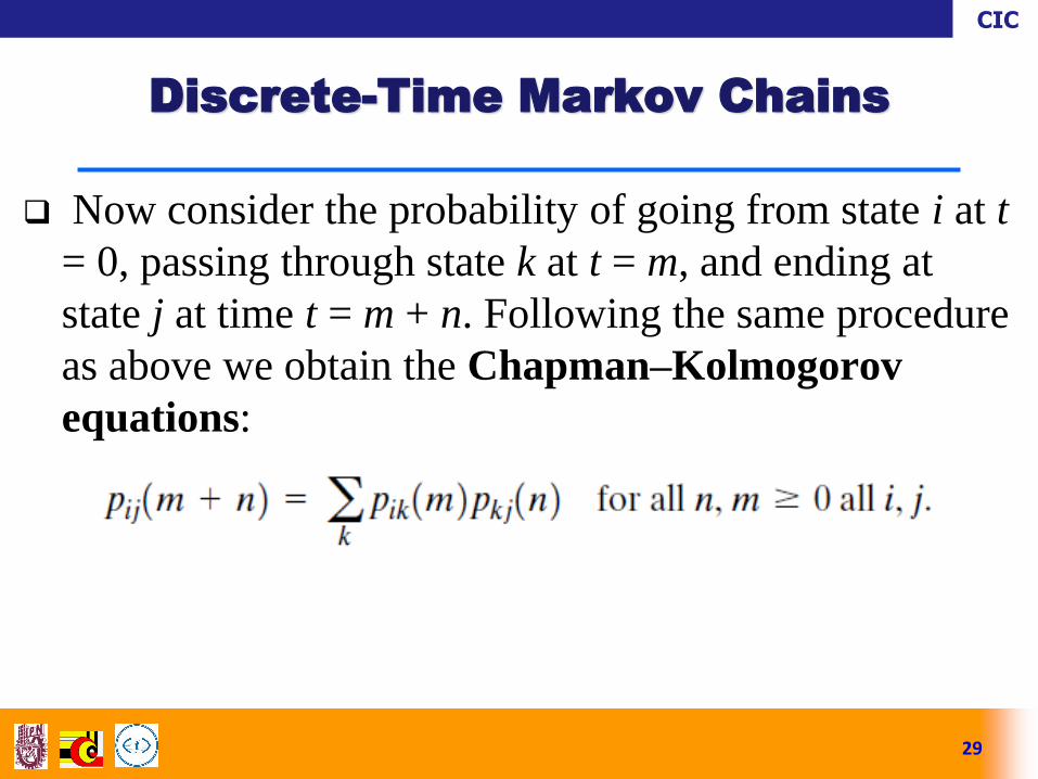
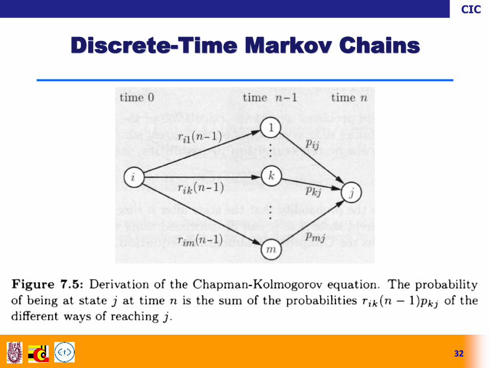
Now consider the probability of going from state i at t
= 0, passing through state k at t = m, and ending at
state j at time t = m + n. Following the same procedure
as above we obtain the Chapman–Kolmogorov
equations:
29
Discrete-Time Markov Chains
CIC
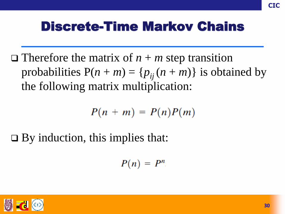
Therefore the matrix of n + m step transition
probabilities P(n + m) = {pij (n + m)} is obtained by
the following matrix multiplication:
By induction, this implies that:
30
Discrete-Time Markov Chains
CIC
31
Discrete-Time Markov Chains
CIC
32
Discrete-Time Markov Chains
CIC
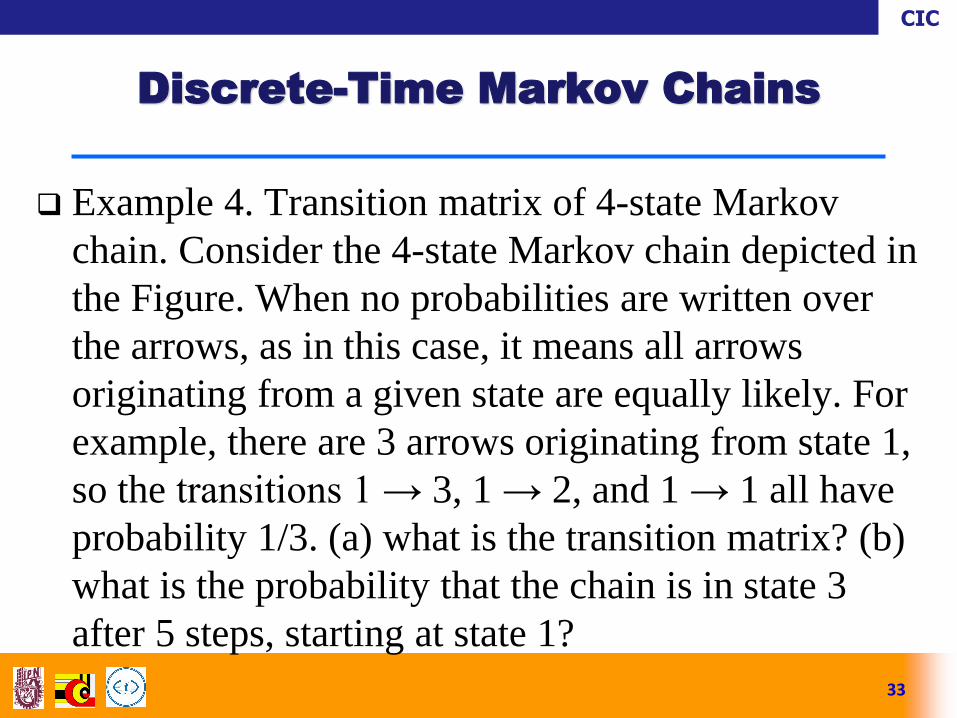
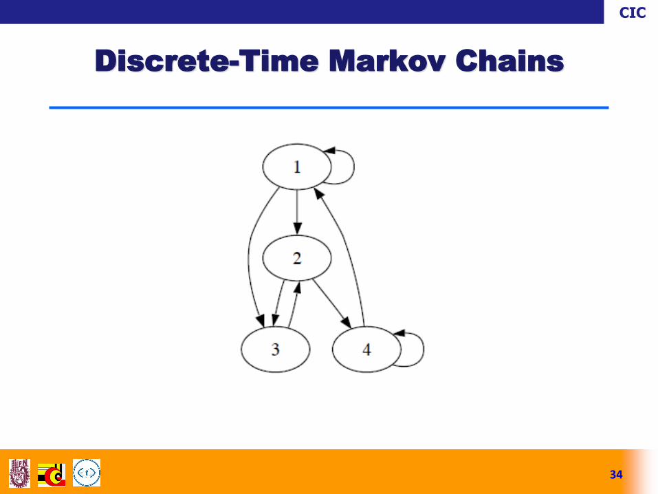
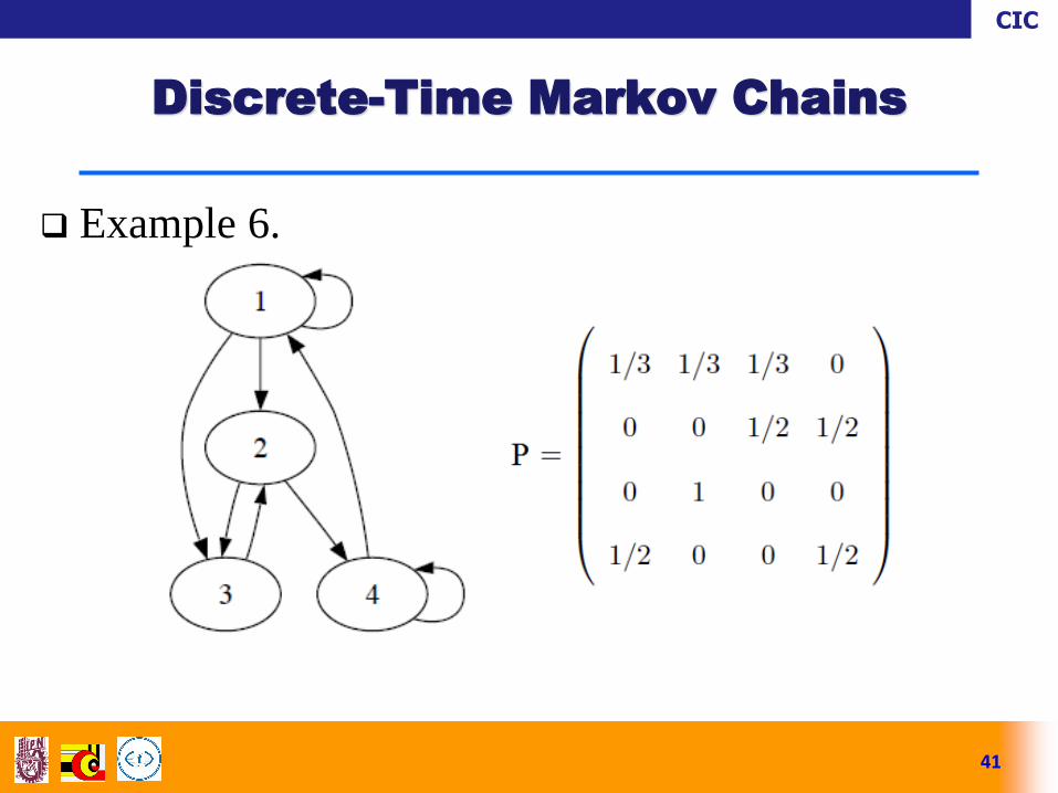
Example 4. Transition matrix of 4-state Markov
chain. Consider the 4-state Markov chain depicted in
the Figure. When no probabilities are written over
the arrows, as in this case, it means all arrows
originating from a given state are equally likely. For
example, there are 3 arrows originating from state 1,
so the transitions 1 → 3, 1 → 2, and 1 → 1 all have
probability 1/3. (a) what is the transition matrix? (b)
what is the probability that the chain is in state 3
after 5 steps, starting at state 1?
33
Discrete-Time Markov Chains
CIC
34
Discrete-Time Markov Chains
CIC
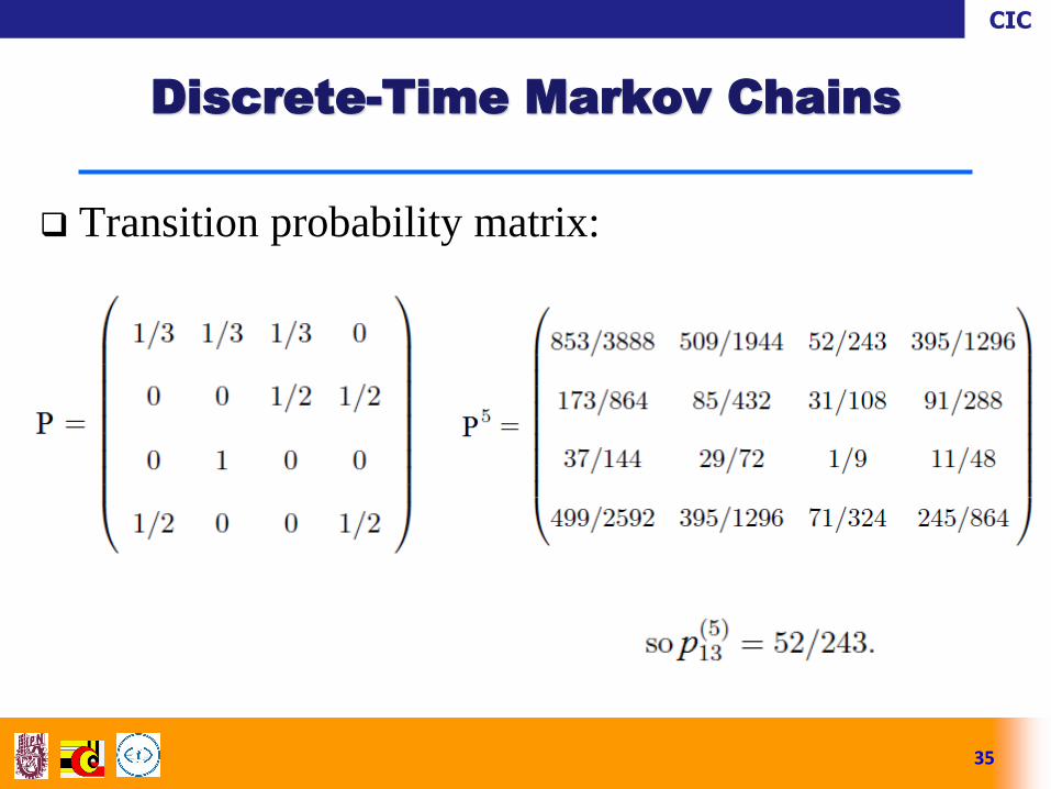
Transition probability matrix:
35
Discrete-Time Markov Chains
CIC
We now consider the long-term behavior of a Markov
chain when it starts in a state chosen by a probability
distribution on the set of states, which we will call a
probability vector.
A probability vector with r components is a row vector
whose entries are non-negative and sum to 1.
If u is a probability vector which represents the initial
state of a Markov chain, then we think of the ith
component of u as representing the probability that the
chain starts in state si.
36
Discrete-Time Markov Chains
CIC
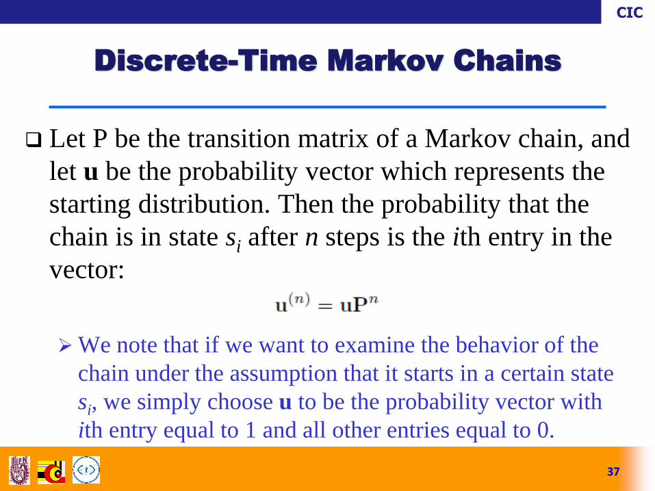
Let P be the transition matrix of a Markov chain, and
let u be the probability vector which represents the
starting distribution. Then the probability that the
chain is in state si after n steps is the ith entry in the
vector:
We note that if we want to examine the behavior of the
chain under the assumption that it starts in a certain state
si, we simply choose u to be the probability vector with
ith entry equal to 1 and all other entries equal to 0.
37
Discrete-Time Markov Chains
CIC
Example 5. In the Land of Oz example (Example 2)
let the initial probability vector u equal (1/3, 1/3,
1/3), meaning that the chain has equal probability of
starting in each of the three states. Calculate the
distribution of the states after three days.
38
Discrete-Time Markov Chains
CIC
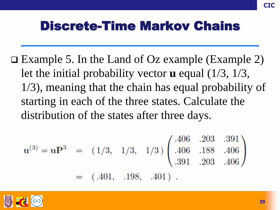
Example 5. In the Land of Oz example (Example 2)
let the initial probability vector u equal (1/3, 1/3,
1/3), meaning that the chain has equal probability of
starting in each of the three states. Calculate the
distribution of the states after three days.
39
Discrete-Time Markov Chains
CIC
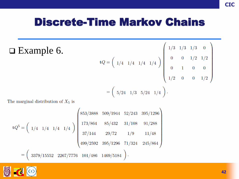
Example 6. Consider the 4-state Markov chain in
Example 4. Suppose the initial conditions are t =
(1/4, 1/4, 1/4, 1/4), meaning that the chain has equal
probability of starting in each of the four states. Let Xn
be the position of the chain at time n. Then the
marginal distribution of X1 is:
40
Discrete-Time Markov Chains
CIC
Example 6.
41
Discrete-Time Markov Chains
CIC
Example 6.
42
Discrete-Time Markov Chains
CIC
The states of a Markov chain can be classified as
recurrent or transient, depending on whether they
are visited over and over again in the long run or are
eventually abandoned.
States can also be classified according to their
period, which is a positive integer summarizing the
amount of time that can elapse between successive
visits to a state.
43
Classification of States
CIC
Recurrent and transient states.
State i of a Markov chain is recurrent if starting from i,
the probability is 1 that the chain will eventually return to
i.
Otherwise, the state is transient, which means that if the
chain starts from i, there is a positive probability of never
returning to i.
As long as there is a positive probability of leaving i
forever, the chain eventually will leave i forever.
44
Classification of States
CIC
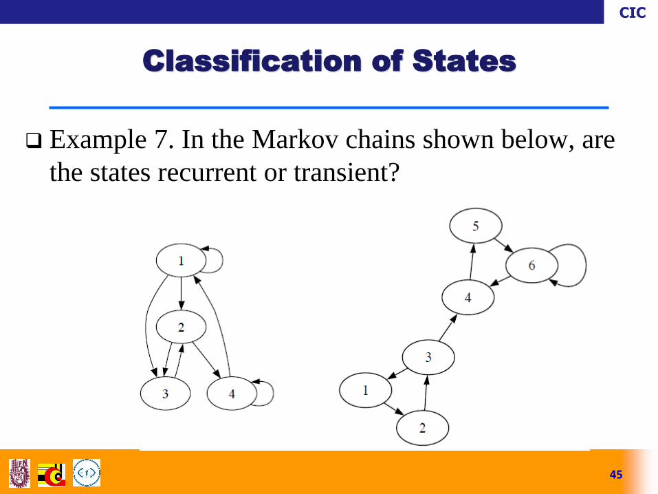
Example 7. In the Markov chains shown below, are
the states recurrent or transient?
45
Classification of States

CIC
Example 7. In the Markov chains shown below, are
the states recurrent or transient?
46
Classification of States
A particle moving around between
states will continue to spend time in
all 4 states in the long run, since it
is possible to get from any state to
any other state.
CIC
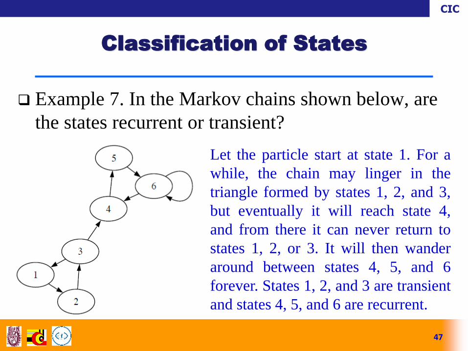
Example 7. In the Markov chains shown below, are
the states recurrent or transient?
47
Classification of States
Let the particle start at state 1. For a
while, the chain may linger in the
triangle formed by states 1, 2, and 3,
but eventually it will reach state 4,
and from there it can never return to
states 1, 2, or 3. It will then wander
around between states 4, 5, and 6
forever. States 1, 2, and 3 are transient
and states 4, 5, and 6 are recurrent.
CIC
Although the definition of a transient state only
requires that there be a positive probability of never
returning to the state, we can say something
stronger:
As long as there is a positive probability of leaving i
forever, the chain eventually will leave i forever.
In the long run, anything that can happen, will happen
(with a finite state space).
48
Classification of States

CIC
If there is a recurrent state, the set of states A(i) that
are accessible from i form a recurrent class (or
simply class), meaning that states in A(i) are all
accessible from each other, and no state outside A(i)
is accessible from them.
A state j is accessible from state i if for some n, the n-step
transition probability pij(n) is positive, i.e., if there is
positive probability of reaching j, starting from i, after
some number of time periods.
49
Classification of States
CIC
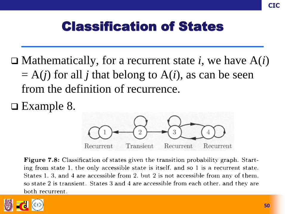
Mathematically, for a recurrent state i, we have A(i)
= A(j) for all j that belong to A(i), as can be seen
from the definition of recurrence.
Example 8.
50
Classification of States
CIC
51
Classification of States
CIC
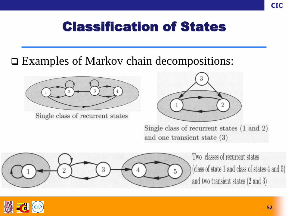
Examples of Markov chain decompositions:
52
Classification of States
CIC
From Markov chain decomposition:
(a) once the state enters (or starts in) a class of recurrent
states, it stays within that class; since all states in the class
are accessible from each other, all states in the class will
be visited an infinite number of times
(b) if the initial state is transient, then the state trajectory
contains an initial portion consisting of transient states
and a final portion consisting of recurrent states from the
same class.
53
Classification of States
CIC
For the purpose of understanding long-term
behaviour of Markov chains, it is important to
analyse chains that consist of a single recurrent
class.
For the purpose of understanding short-term
behaviour, it is also important to analyse the
mechanism by which any particular class of
recurrent states is entered starting from a given
transient state.
54
Classification of States
CIC
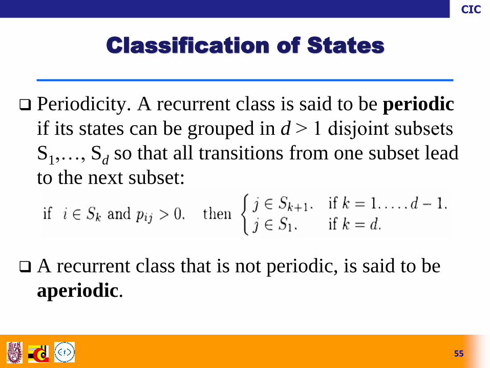
Periodicity. A recurrent class is said to be periodic
if its states can be grouped in d ˃ 1 disjoint subsets
S1,…, Sd so that all transitions from one subset lead
to the next subset:
A recurrent class that is not periodic, is said to be
aperiodic.
55
Classification of States

CIC
In a periodic recurrent class, we move through the
sequence of subsets in order, and after d steps, we
end up in the same subset.
Example:
56
Classification of States
CIC
Irreducible and reducible chain. A Markov chain
with transition matrix P is irreducible if for any two
states i and j, it is possible to go from i to j in a finite
number of steps (with positive probability). That is,
for any states i, j there is some positive integer n
such that the (i, j) entry of Pn is positive. A Markov
chain that is not irreducible is called reducible.
In an irreducible Markov chain with a finite state space,
all states are recurrent.
57
Classification of States
CIC
Example 8. Gambler’s ruin as a Markov chain. In
the gambler’s ruin problem, two gamblers, A and B,
start with i and N − i dollars respectively, making a
sequence of bets for $1. In each round, player A has
probability p of winning and probability q = 1− p of
losing. Let Xn be the wealth of gambler A at time n.
Then X0, X1, . . . is a Markov chain on the state
space {0, 1, . . . ,N}. By design, X0 = i. Draw the
transition probability graph.
58
Classification of States
CIC
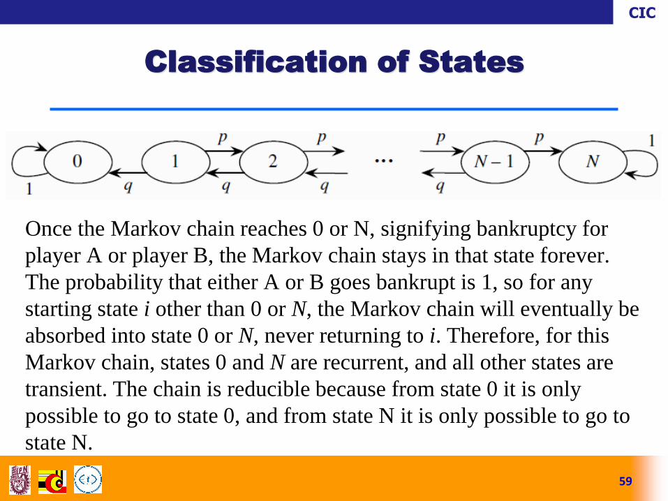
Once the Markov chain reaches 0 or N, signifying bankruptcy for
player A or player B, the Markov chain stays in that state forever.
The probability that either A or B goes bankrupt is 1, so for any
starting state i other than 0 or N, the Markov chain will eventually be
absorbed into state 0 or N, never returning to i. Therefore, for this
Markov chain, states 0 and N are recurrent, and all other states are
transient. The chain is reducible because from state 0 it is only
possible to go to state 0, and from state N it is only possible to go to
state N.
59
Classification of States
CIC
The concepts of recurrence and transience are
important for understanding the long-run behavior of
a Markov chain.
At first, the chain may spend time in transient states.
Eventually though, the chain will spend all its time in
recurrent states. But what fraction of the time will it spend
in each of the recurrent states?
This question is answered by the stationary
distribution of the chain, also known as the steady-
state behaviour.
60
Steady State Behaviour
CIC
In Markov chain models, it is interesting to
determine the long-term state occupancy behaviour
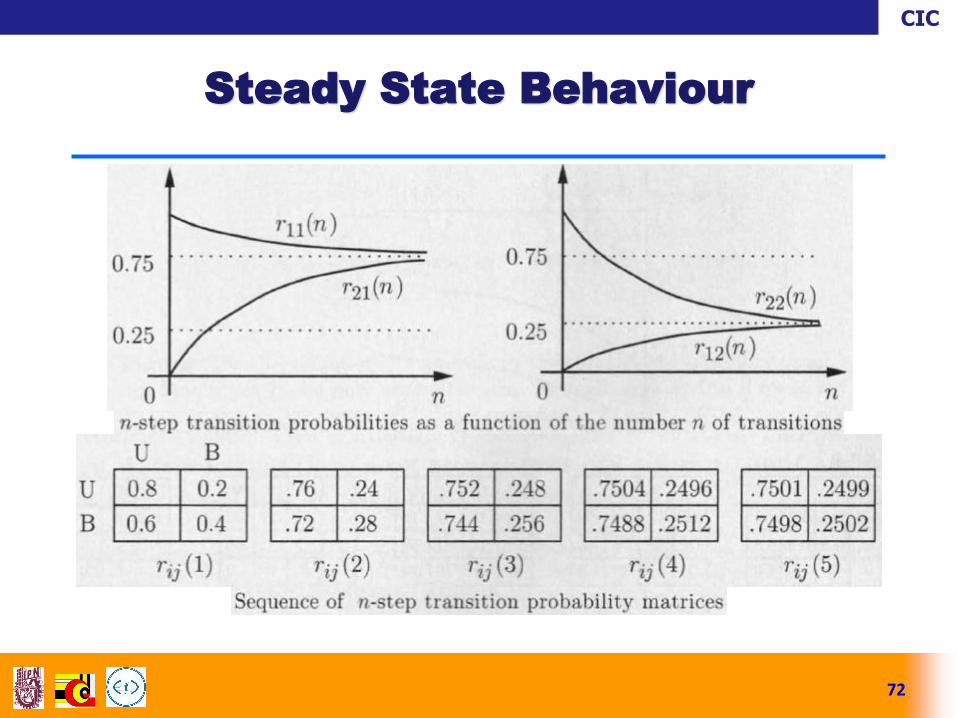
in the n-step transition probabilities pij when n is very
large.
pij may converge to steady-state values that are
independent of the initial state.
For every state j, the probability pij(n) of being at state j
approaches a limiting value that is independent of the
initial state i, provided we exclude two situations,
multiple recurrent classes/or a periodic class.
61
Steady State Behaviour
CIC
This limiting value, denoted as j , has the
interpretation:
And is called the steady-state probability of j.
62
Steady State Behaviour

CIC
Consider a Markov chain with a single recurrent class, which is
aperiodic. Then, the states j are associated with steady-state
probabilities j that have the following properties:
(a) For each j, we have:
(b) The j are the unique solution to the system of equations below:
(c) We have:
63
Steady-State Convergence Theorem
CIC
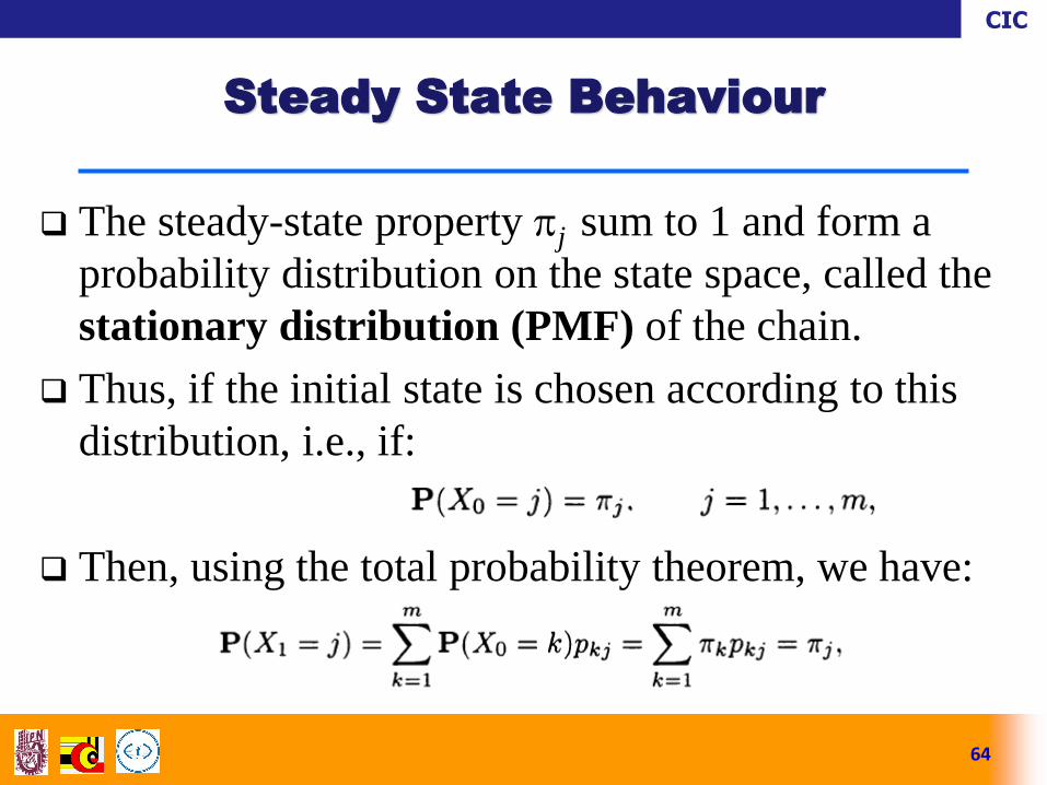
The steady-state property j sum to 1 and form a
probability distribution on the state space, called the
stationary distribution (PMF) of the chain.
Thus, if the initial state is chosen according to this
distribution, i.e., if:
Then, using the total probability theorem, we have:
64
Steady State Behaviour
CIC
where the last equation follows from part (b) of the
steady-state theorem.
Similarly, we obtain P(Xn = j) = j, for all n and j.
Thus, if the initial state is chosen according to the
stationary distribution, the state at any future time
will have the same distribution.
65
Steady State Behaviour
CIC
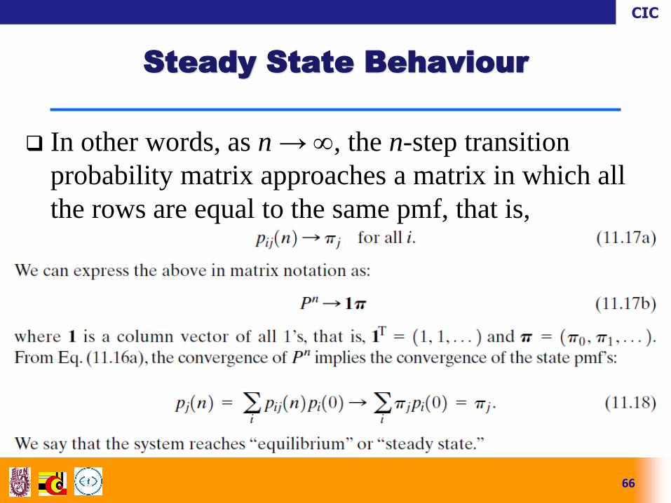
In other words, as n → , the n-step transition
probability matrix approaches a matrix in which all
the rows are equal to the same pmf, that is,
66
Steady State Behaviour
CIC
67
Steady State Behaviour
CIC
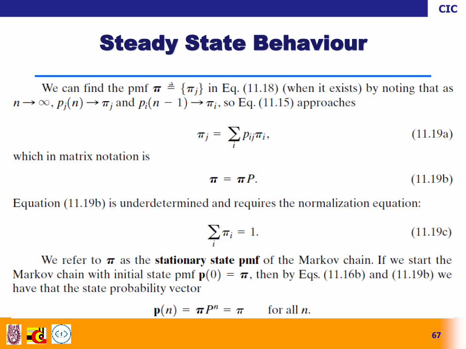
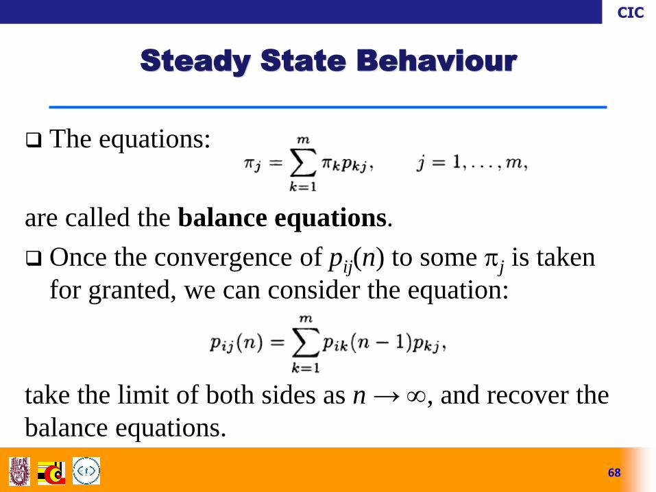
The equations:
are called the balance equations.
Once the convergence of pij(n) to some j is taken
for granted, we can consider the equation:
take the limit of both sides as n → , and recover the
balance equations.
68
Steady State Behaviour
CIC
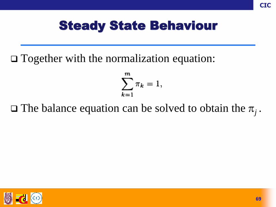
Together with the normalization equation:
The balance equation can be solved to obtain the j .
69
Steady State Behaviour
CIC
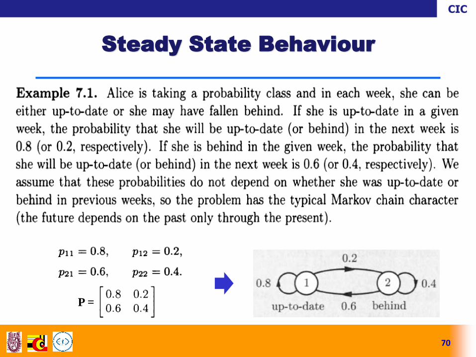
70
Steady State Behaviour
P =
CIC
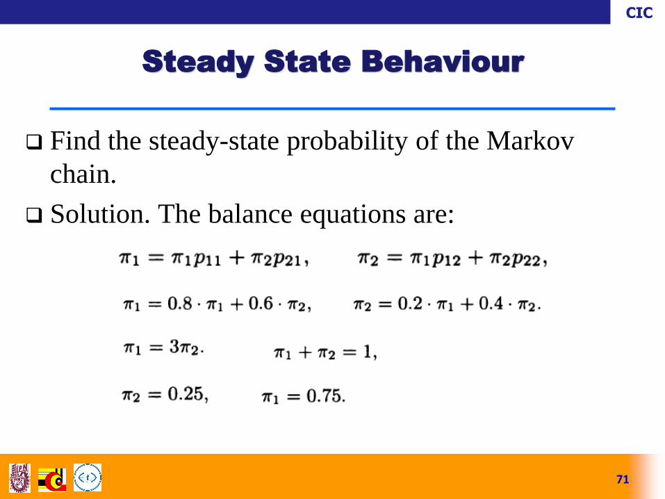
Find the steady-state probability of the Markov
chain.
Solution. The balance equations are:
71
Steady State Behaviour
CIC
72
Steady State Behaviour
CIC
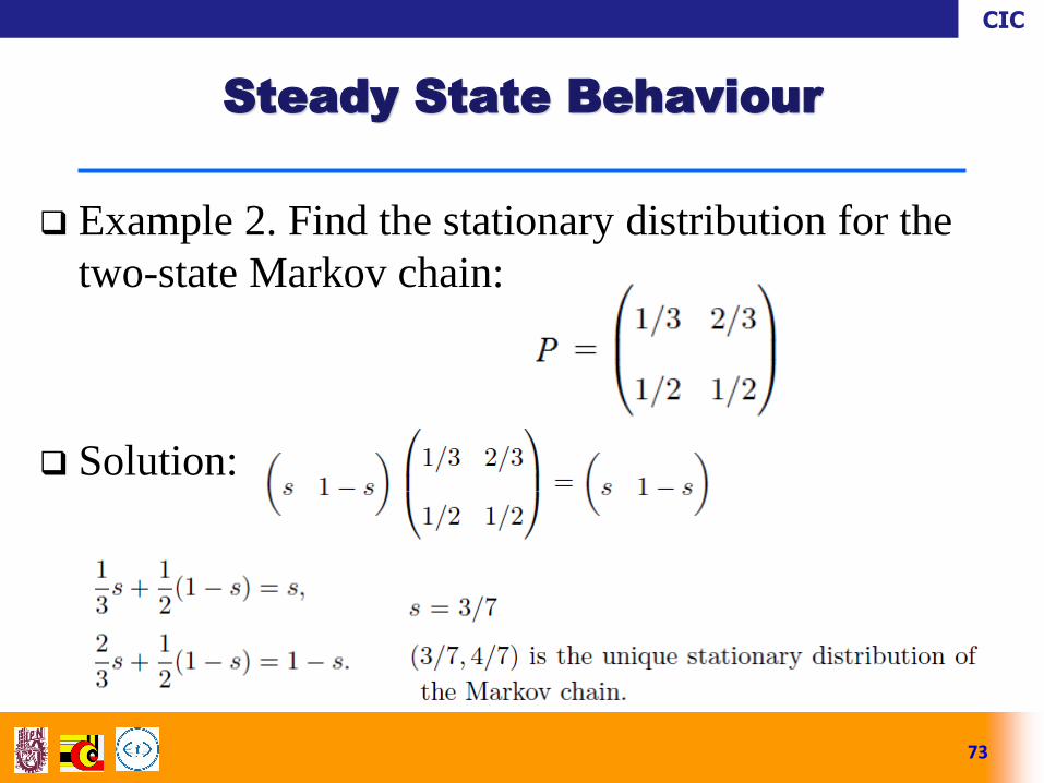
Example 2. Find the stationary distribution for the
two-state Markov chain:
Solution:
73
Steady State Behaviour
CIC
One way to visualize the stationary distribution of a
Markov chain is to imagine a large number of particles,
each independently bouncing from state to state according
to the transition probabilities. After a while, the system of
particles will approach an equilibrium where, at each time
period, the number of particles leaving a state will be
counterbalanced by the number of particles entering that
state, and this will be true for all states. As a result, the
system as a whole will appear to be stationary, and the
proportion of particles in each state will be given by the
stationary distribution.
74
Steady State Behaviour
CIC
Consider, for example, a Markov chain involving a
machine, which at the end of any day can be in one of
two states, working or broken down. Each time it brakes
down, it is immediately repaired at a cost of $1. How are
we to model the long-term expected cost of repair per
day?
View it as the expected value of the repair cost on a randomly
chosen day far into the future; this is just the steady-state
probability of the broken down state.
Calculate the total expected repair cost in n days, where n is
very large, and divide it by n.
75
Long-Term Frequency
Interpretation
CIC
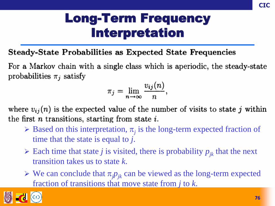
Based on this interpretation, j is the long-term expected fraction of
time that the state is equal to j.
Each time that state j is visited, there is probability pjk that the next
transition takes us to state k.
We can conclude that jpjk can be viewed as the long-term expected
fraction of transitions that move state from j to k.
76
Long-Term Frequency
Interpretation
CIC
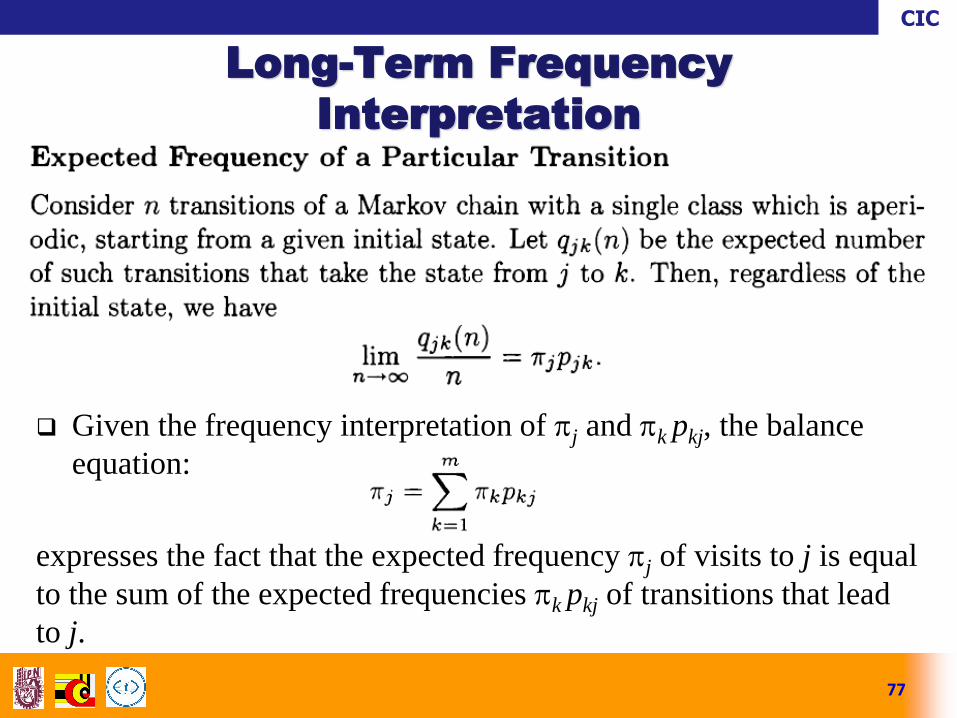
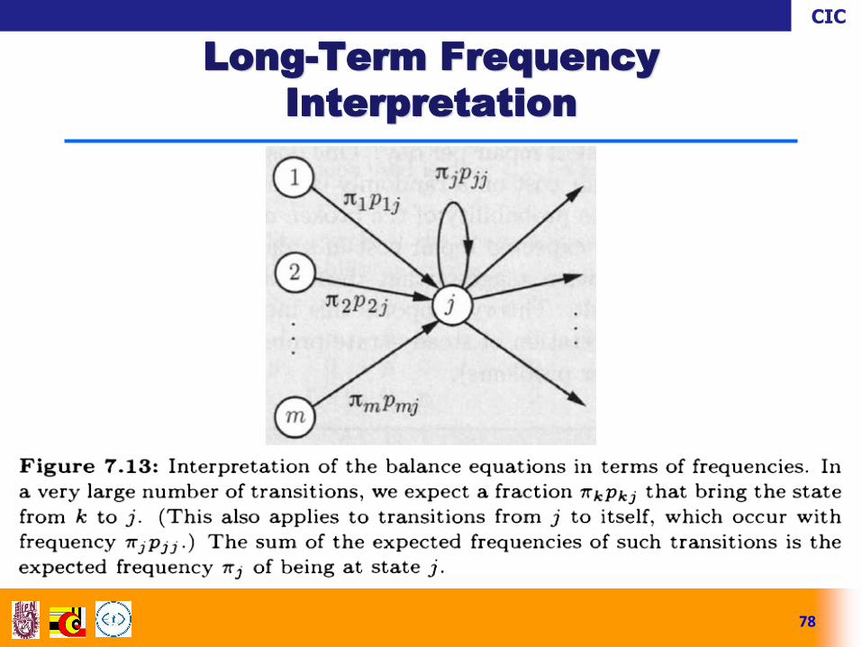
Given the frequency interpretation of j and k pkj, the balance
equation:
expresses the fact that the expected frequency j of visits to j is equal
to the sum of the expected frequencies k pkj of transitions that lead
to j.
77
Long-Term Frequency
Interpretation
CIC
78
Long-Term Frequency
Interpretation
CIC
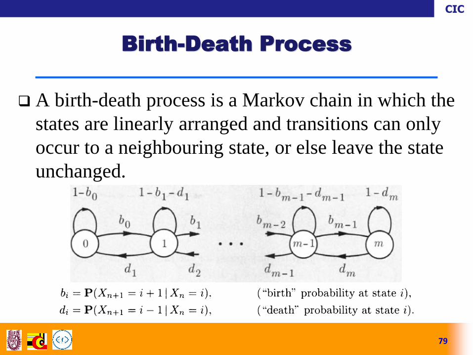
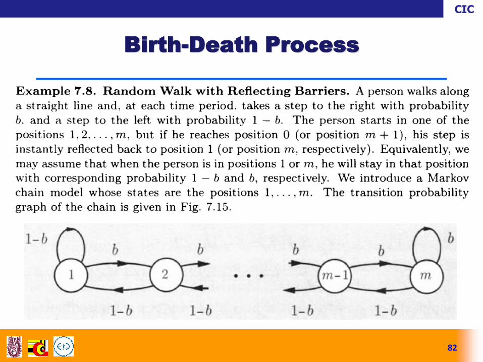
A birth-death process is a Markov chain in which the
states are linearly arranged and transitions can only
occur to a neighbouring state, or else leave the state
unchanged.
79
Birth-Death Process
CIC
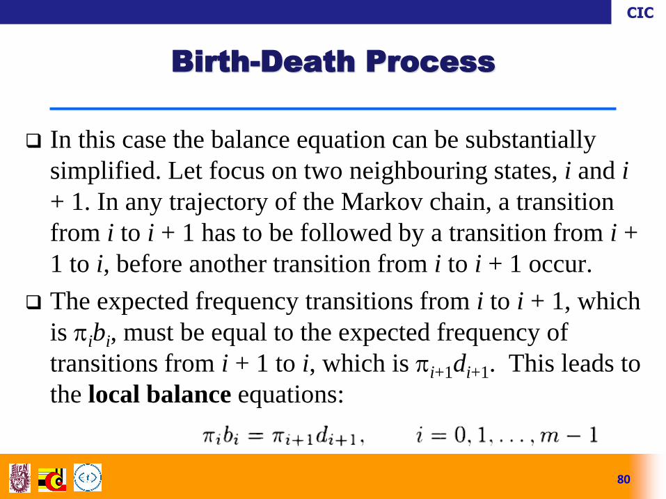
In this case the balance equation can be substantially
simplified. Let focus on two neighbouring states, i and i
+ 1. In any trajectory of the Markov chain, a transition
from i to i + 1 has to be followed by a transition from i +
1 to i, before another transition from i to i + 1 occur.
The expected frequency transitions from i to i + 1, which
is ibi, must be equal to the expected frequency of
transitions from i + 1 to i, which is i+1di+1. This leads to
the local balance equations:
80
Birth-Death Process
CIC
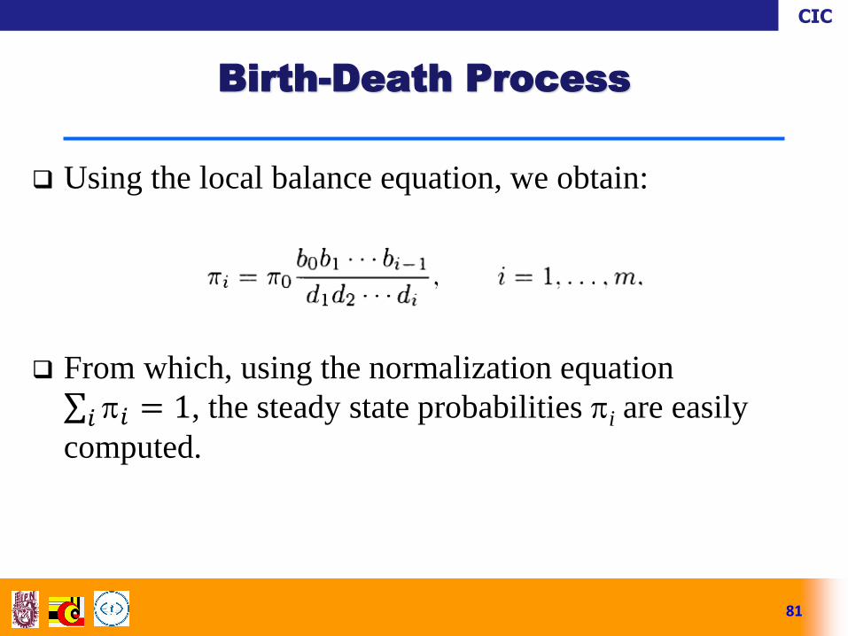
Using the local balance equation, we obtain:
From which, using the normalization equation
𝑖 = 1𝑖 , the steady state probabilities i are easily
computed.
81
Birth-Death Process
CIC
82
Birth-Death Process
CIC
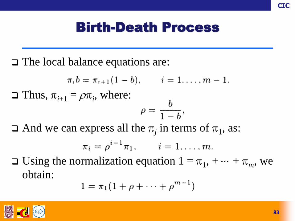
The local balance equations are:
Thus, i+1 = i, where:
And we can express all the j in terms of 1, as:
Using the normalization equation 1 = 1, + + m, we
obtain:
83
Birth-Death Process
CIC
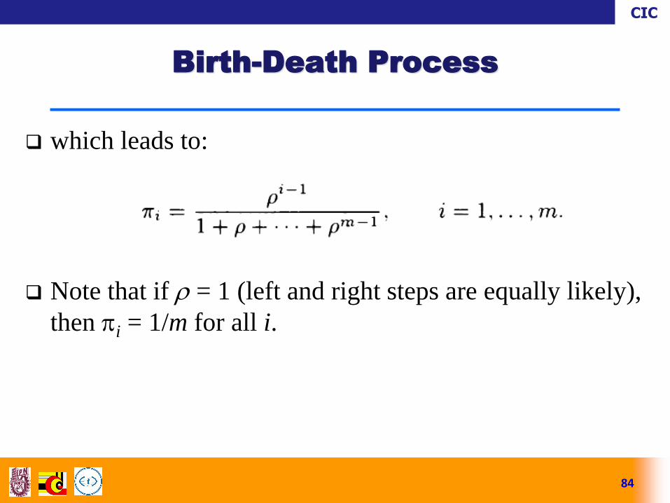
which leads to:
Note that if = 1 (left and right steps are equally likely),
then i = 1/m for all i.
84
Birth-Death Process
CIC
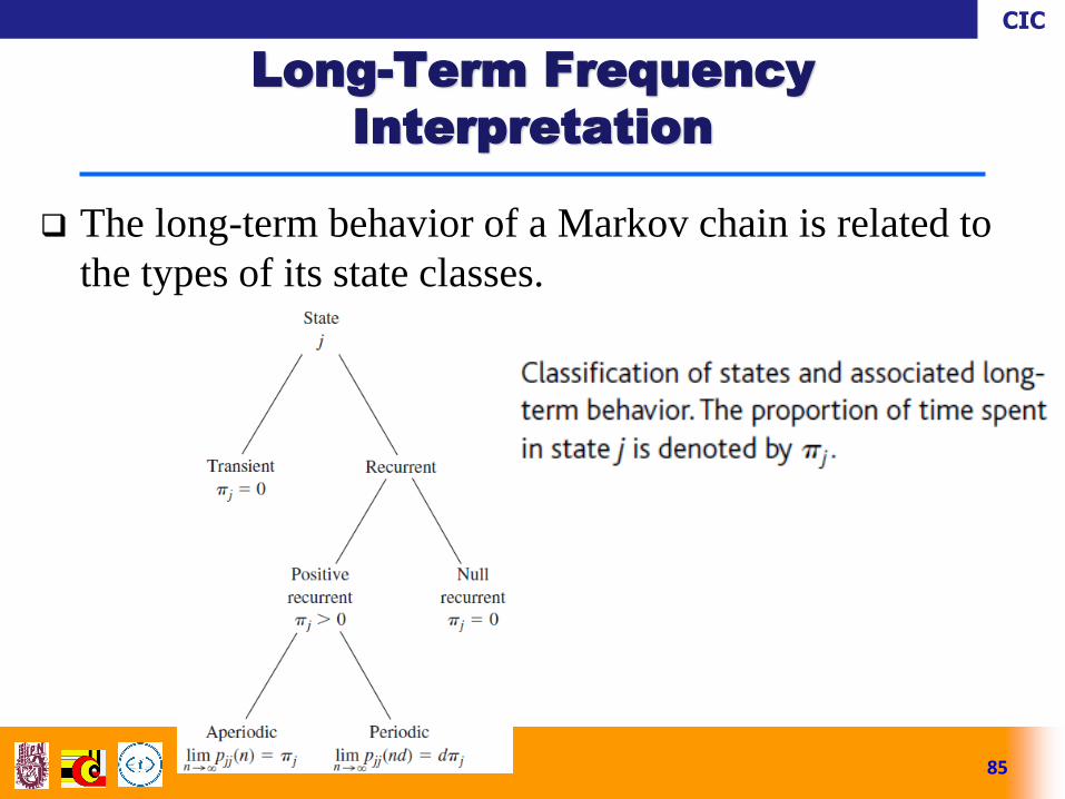
The long-term behavior of a Markov chain is related to
the types of its state classes.
85
Long-Term Frequency
Interpretation
CIC
What is the short-time behaviour of Markov
chains??
Consider the case where the Markov chain starts at a
transient state.
We are interested in the first recurrent state to be entered,
as well as in the time until this happens.
When addressing such questions, the subsequent
behaviour of the Markov chain (after a recurrent
state is encountered) is immaterial.
86
Absorption Probabilities and
Expected Time to Absorption
CIC
Focusing on the case where every recurrent state k is
absorbing, i.e.,
If there is a unique absorbing state k, its steady-state
probability is 1, and will be reached with probability
1, starting from any initial state.
Because all other states are transient and have zero
steady-state probability.
87
Absorption Probabilities
CIC
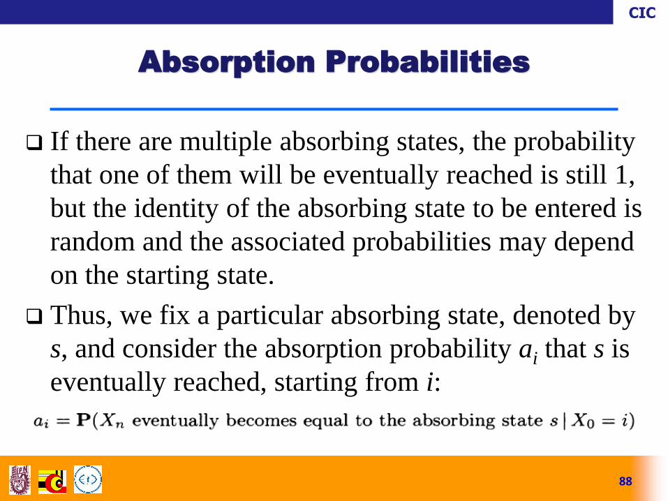
If there are multiple absorbing states, the probability
that one of them will be eventually reached is still 1,
but the identity of the absorbing state to be entered is
random and the associated probabilities may depend
on the starting state.
Thus, we fix a particular absorbing state, denoted by
s, and consider the absorption probability ai that s is
eventually reached, starting from i:
88
Absorption Probabilities
CIC
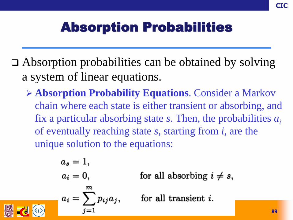
Absorption probabilities can be obtained by solving
a system of linear equations.
Absorption Probability Equations. Consider a Markov
chain where each state is either transient or absorbing, and
fix a particular absorbing state s. Then, the probabilities ai
of eventually reaching state s, starting from i, are the
unique solution to the equations:
89
Absorption Probabilities
CIC
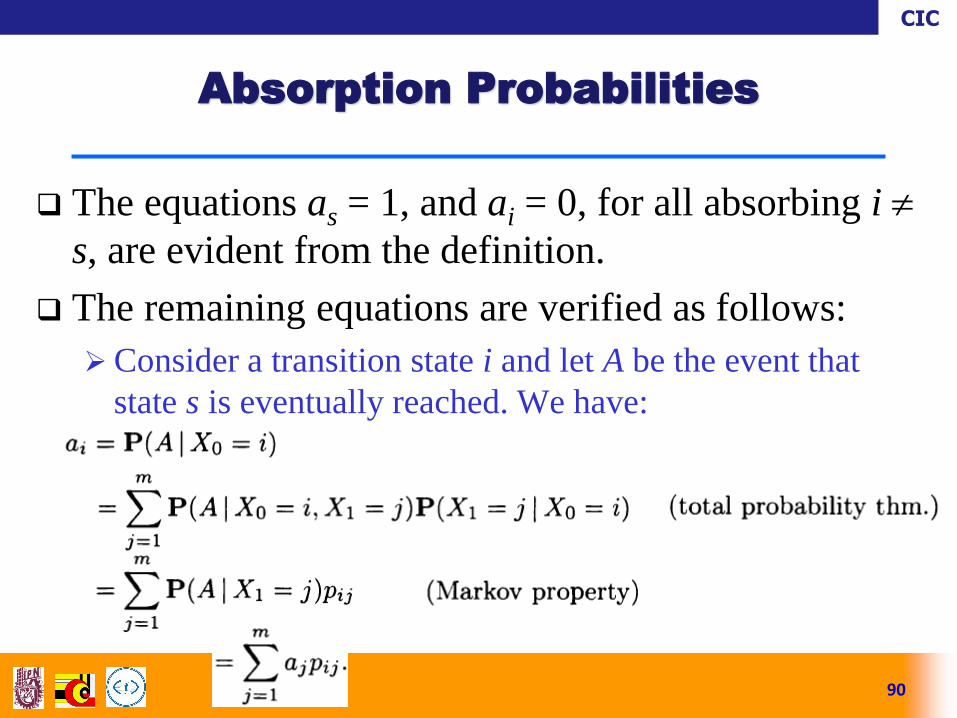
The equations as = 1, and ai = 0, for all absorbing i
s, are evident from the definition.
The remaining equations are verified as follows:
Consider a transition state i and let A be the event that
state s is eventually reached. We have:
90
Absorption Probabilities
CIC
91
Absorption Probabilities
CIC
92
Absorption Probabilities
CIC
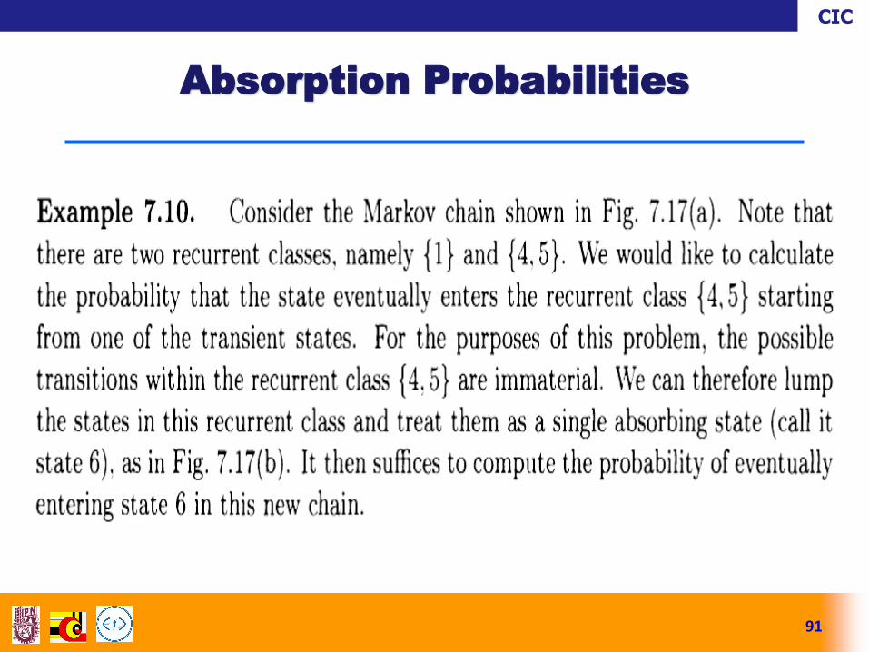
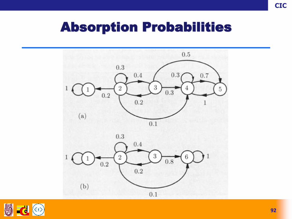
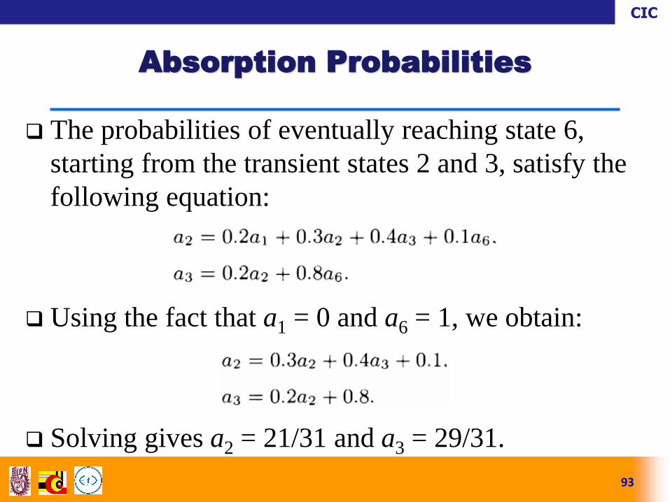
The probabilities of eventually reaching state 6,
starting from the transient states 2 and 3, satisfy the
following equation:
Using the fact that a1 = 0 and a6 = 1, we obtain:
Solving gives a2 = 21/31 and a3 = 29/31.
93
Absorption Probabilities
CIC
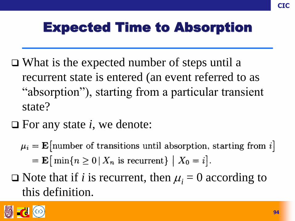
What is the expected number of steps until a
recurrent state is entered (an event referred to as
“absorption”), starting from a particular transient
state?
For any state i, we denote:
Note that if i is recurrent, then i = 0 according to
this definition.
94
Expected Time to Absorption
CIC
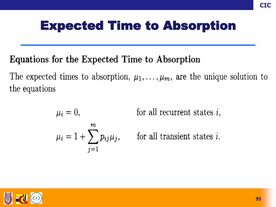
95
Expected Time to Absorption

CIC
Calculate the expected number of steps until the fly is captured.
96
Expected Time to Absorption
CIC
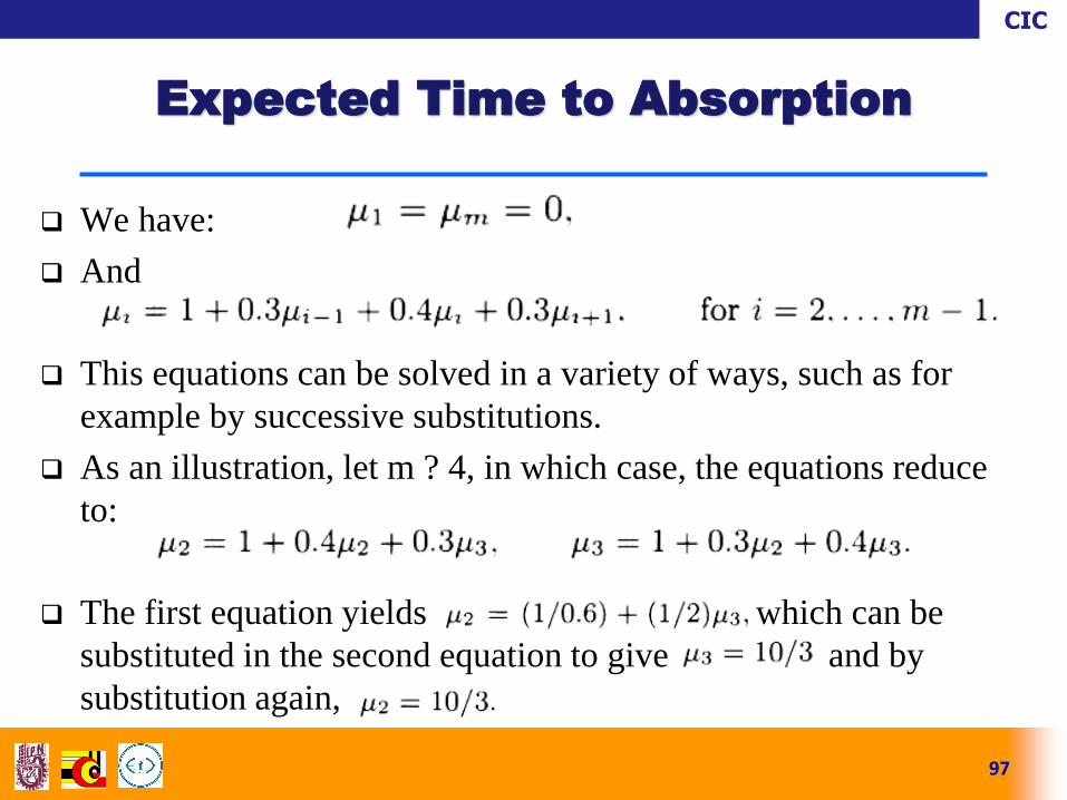
We have:
And
This equations can be solved in a variety of ways, such as for
example by successive substitutions.
As an illustration, let m ? 4, in which case, the equations reduce
to:
The first equation yields which can be
substituted in the second equation to give and by
substitution again,
97
Expected Time to Absorption
CIC
The idea used to calculate the expected time to
absorption can also be used to calculate the expected
time to reach a particular recurrent state, starting
from any other state.
For simplicity, consider a Markov chain with a
single recurrent class.
98
Mean First Passage and Recurrence
Times
CIC
Let focus on a special recurrent state s, and denote
by ti the mean first passage time from state i to
state s, defined by:
The transition out of state s are irrelevant to the
calculation of the mean first passage times.
99
Mean First Passage and Recurrence
Times
CIC
Consider thus a new Markov chain which is identical
to the original, except that the special state s is
converted into an absorbing state (by setting pss = 1,
and psj = 0 for all j s).
Whit this transformation, all states other than s
become transient.
100
Mean First Passage and Recurrence
Times
CIC
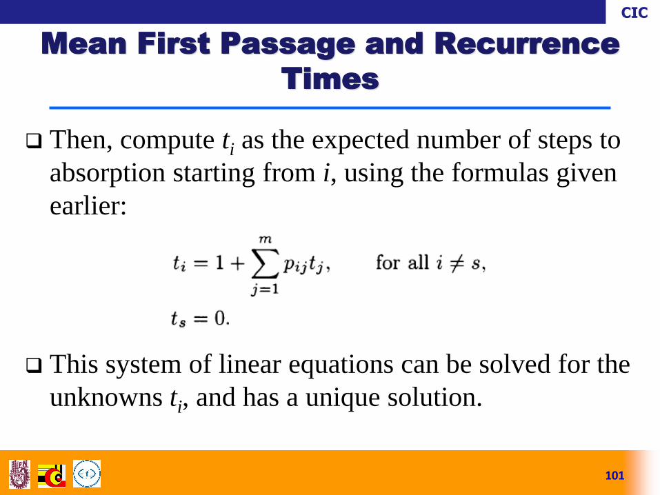
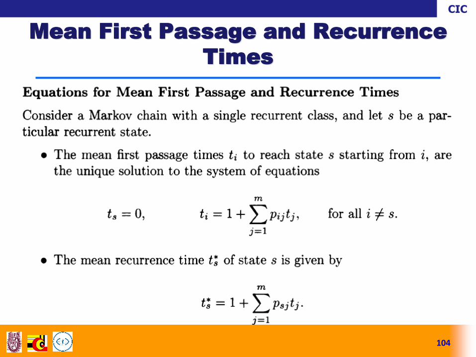
Then, compute ti as the expected number of steps to
absorption starting from i, using the formulas given
earlier:
This system of linear equations can be solved for the
unknowns ti, and has a unique solution.
101
Mean First Passage and Recurrence
Times
CIC
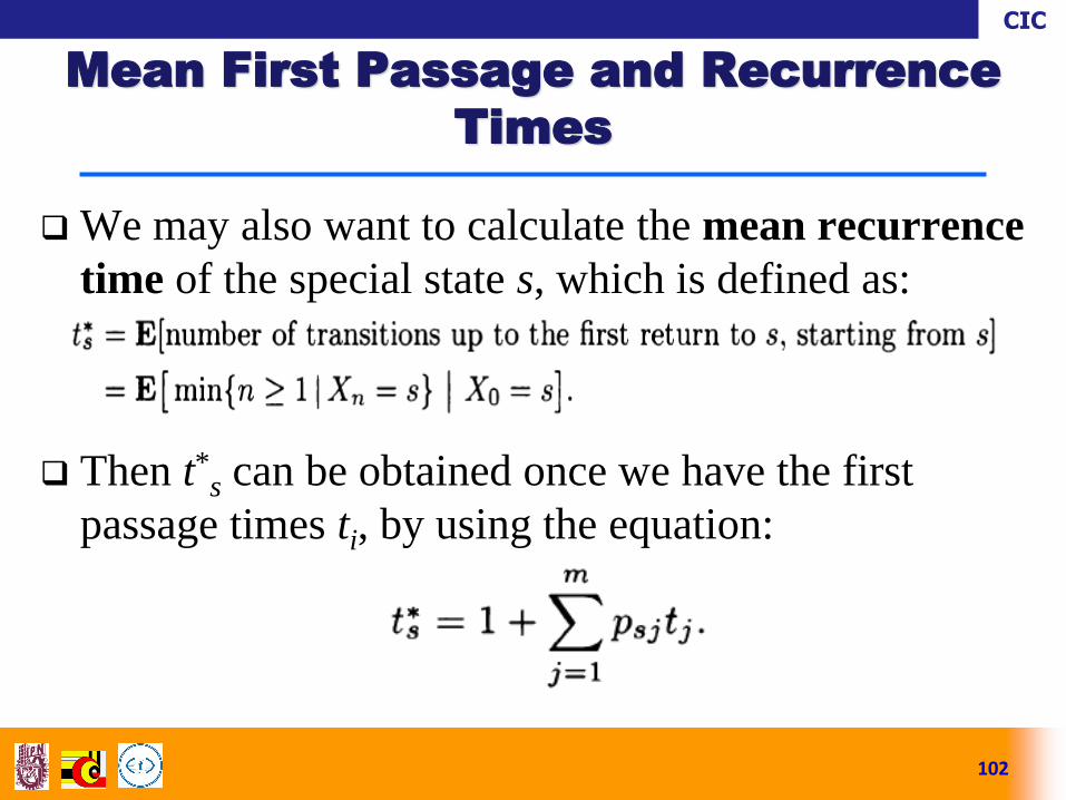
We may also want to calculate the mean recurrence
time of the special state s, which is defined as:
Then t*s can be obtained once we have the first
passage times ti, by using the equation:
102
Mean First Passage and Recurrence
Times
CIC
This equation can be justified saying that the time to
return to s, starting from s, is equal to 1 plus the
expected time to reach s from the next state, which is
j with probability psj. Then apply the total
expectation theorem.
103
Mean First Passage and Recurrence
Times
CIC
104
Mean First Passage and Recurrence
Times
CIC
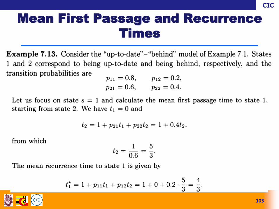
105
Mean First Passage and Recurrence
Times
CIC
In discrete Markov chains models it is assumed that
the transitions between states take unit time.
Continuous time Markov chains evolve in
continuous time.
Can be used to study systems involving continuous-time
arrival processes.
Examples: Distribution centres or nodes in
communication networks where some events of interest
are described in terms of Poisson processes.
106
Continuous Time Markov Chains
CIC
Similar to the discrete Markov chains, continuous
time Markov chains involve transitions from one
state to the next:
According to a given transition probabilities
The time spend between transitions is modelled as
continuous random variables.
It is assumed that the number of states is finite
In absence of a statement to the contrary, the state space is
the set S = {1,…, m}.
107
Continuous Time Markov Chains
CIC
To describe a continuous Markov chain, some
random variables of interest are introduced:
For completeness, X0 denotes the initial state, and
Y0 = 0.
108
Continuous Time Markov Chains
CIC
109
Continuous Time Markov Chains
CIC
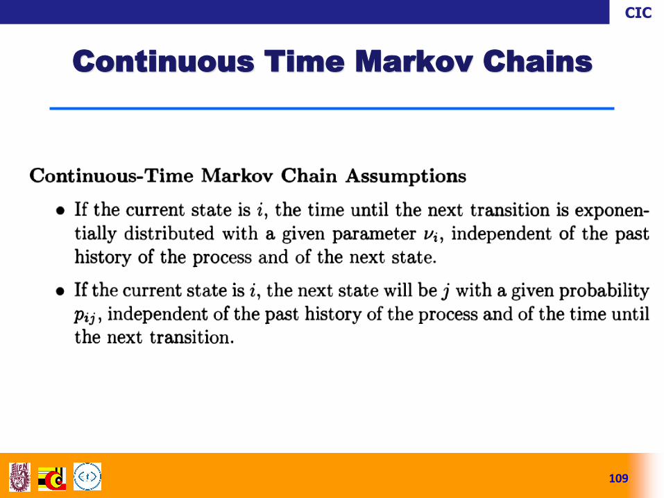
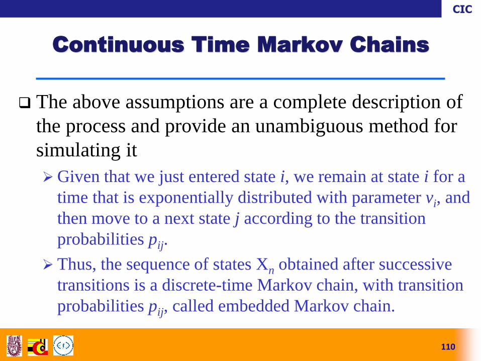
The above assumptions are a complete description of
the process and provide an unambiguous method for
simulating it
Given that we just entered state i, we remain at state i for a
time that is exponentially distributed with parameter vi, and
then move to a next state j according to the transition
probabilities pij.
Thus, the sequence of states Xn obtained after successive
transitions is a discrete-time Markov chain, with transition
probabilities pij, called embedded Markov chain.
110
Continuous Time Markov Chains
CIC
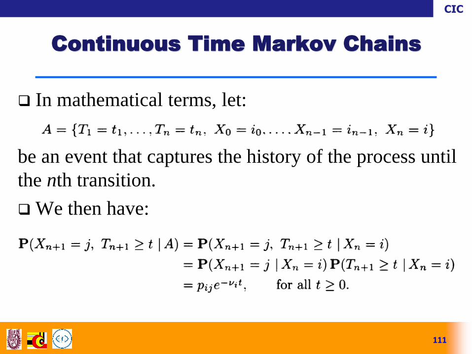
In mathematical terms, let:
be an event that captures the history of the process until
the nth transition.
We then have:
111
Continuous Time Markov Chains
CIC
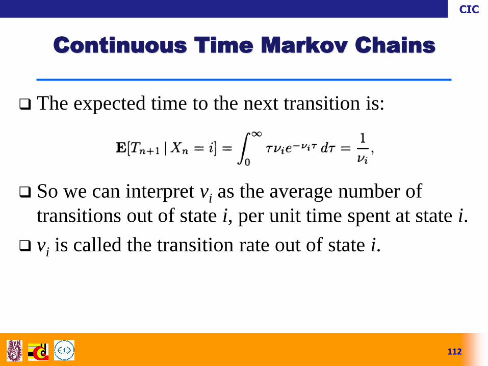
The expected time to the next transition is:
So we can interpret vi as the average number of
transitions out of state i, per unit time spent at state i.
vi is called the transition rate out of state i.
112
Continuous Time Markov Chains
CIC
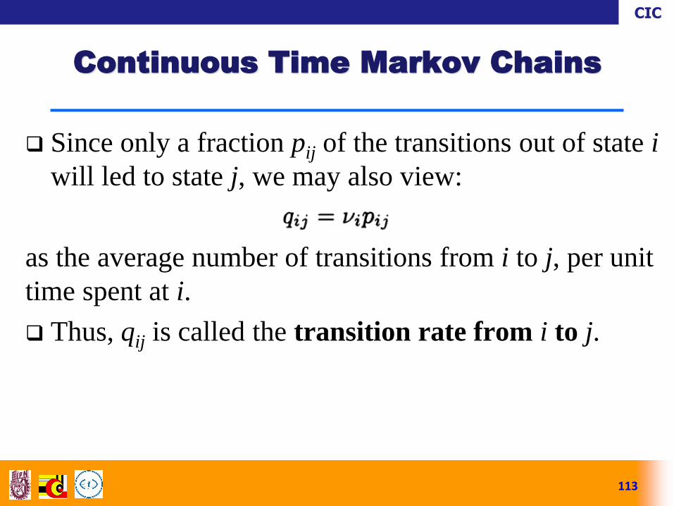
Since only a fraction pij of the transitions out of state i
will led to state j, we may also view:
as the average number of transitions from i to j, per unit
time spent at i.
Thus, qij is called the transition rate from i to j.
113
Continuous Time Markov Chains
CIC
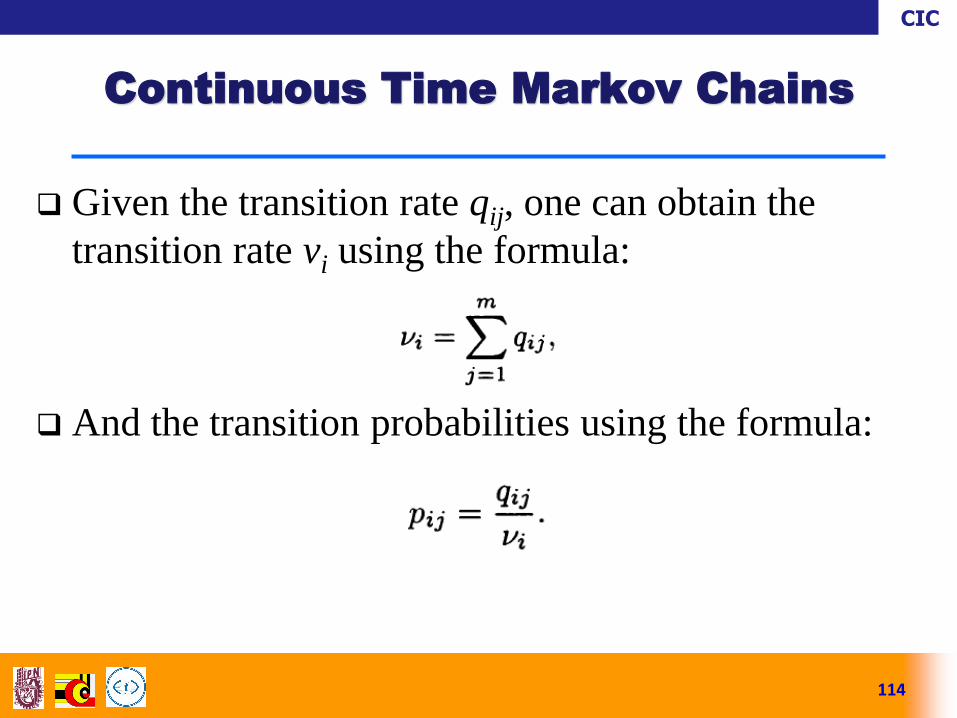
Given the transition rate qij, one can obtain the
transition rate vi using the formula:
And the transition probabilities using the formula:
114
Continuous Time Markov Chains
CIC
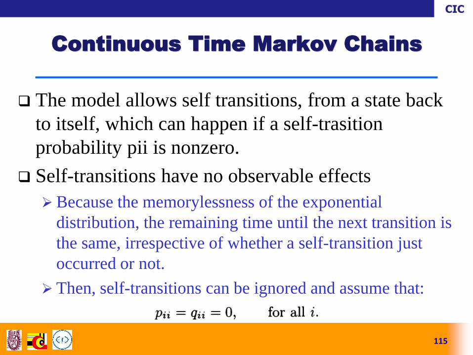
The model allows self transitions, from a state back
to itself, which can happen if a self-trasition
probability pii is nonzero.
Self-transitions have no observable effects
Because the memorylessness of the exponential
distribution, the remaining time until the next transition is
the same, irrespective of whether a self-transition just
occurred or not.
Then, self-transitions can be ignored and assume that:
115
Continuous Time Markov Chains
CIC
116
Continuous Time Markov Chains
CIC
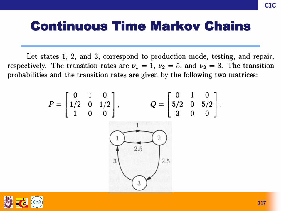
117
Continuous Time Markov Chains
CIC
118
Continuous Time Markov Chains
Similar to its discrete-time counterpart, the
continuous-time process has a Markov property: the
future is independent of the past, given the present.
CIC
119
Ergodic Theorem for Discrete
Markov Chains

CIC
120
Markov Chain Montecarlo Method
CIC
121
Queuing Theory