probability and stochastic processes - semantic scholar · probability and stochastic processes a...
TRANSCRIPT

Probability and Stochastic ProcessesA Friendly Introduction for Electrical and Computer Engineers
Second Edition
Quiz Solutions
Roy D. Yates and David J. Goodman
May 22, 2004
• The MATLAB section quizzes at the end of each chapter use programs available fordownload as the archive matcode.zip. This archive has programs of general pur-pose programs for solving probability problems as well as specific .m files associatedwith examples or quizzes in the text. Also available is a manual probmatlab.pdfdescribing the general purpose .m files in matcode.zip.
• We have made a substantial effort to check the solution to every quiz. Nevertheless,there is a nonzero probability (in fact, a probability close to unity) that errors will befound. If you find errors or have suggestions or comments, please send email to
When errors are found, corrected solutions will be posted at the website.
1

Quiz Solutions – Chapter 1
Quiz 1.1In the Venn diagrams for parts (a)-(g) below, the shaded area represents the indicated
set.
M O
T
M O
T
M O
T
(1) R = T c (2) M ∪ O (3) M ∩ O
M O
T
M O
T
M O
T
(4) R ∪ M (4) R ∩ M (6) T c − M
Quiz 1.2
(1) A1 = {vvv, vvd, vdv, vdd}(2) B1 = {dvv, dvd, ddv, ddd}(3) A2 = {vvv, vvd, dvv, dvd}(4) B2 = {vdv, vdd, ddv, ddd}(5) A3 = {vvv, ddd}(6) B3 = {vdv, dvd}(7) A4 = {vvv, vvd, vdv, dvv, vdd, dvd, ddv}(8) B4 = {ddd, ddv, dvd, vdd}
Recall that Ai and Bi are collectively exhaustive if Ai ∪ Bi = S. Also, Ai and Bi aremutually exclusive if Ai ∩ Bi = φ. Since we have written down each pair Ai and Bi above,we can simply check for these properties.
The pair A1 and B1 are mutually exclusive and collectively exhaustive. The pair A2 andB2 are mutually exclusive and collectively exhaustive. The pair A3 and B3 are mutuallyexclusive but not collectively exhaustive. The pair A4 and B4 are not mutually exclusivesince dvd belongs to A4 and B4. However, A4 and B4 are collectively exhaustive.
2

Quiz 1.3There are exactly 50 equally likely outcomes: s51 through s100. Each of these outcomes
has probability 0.02.
(1) P[{s79}] = 0.02
(2) P[{s100}] = 0.02
(3) P[A] = P[{s90, . . . , s100}] = 11× 0.02 = 0.22
(4) P[F] = P[{s51, . . . , s59}] = 9× 0.02 = 0.18
(5) P[T ≥ 80] = P[{s80, . . . , s100}] = 21× 0.02 = 0.42
(6) P[T < 90] = P[{s51, s52, . . . , s89}] = 39× 0.02 = 0.78
(7) P[a C grade or better] = P[{s70, . . . , s100}] = 31× 0.02 = 0.62
(8) P[student passes] = P[{s60, . . . , s100}] = 41× 0.02 = 0.82
Quiz 1.4We can describe this experiment by the event space consisting of the four possible
events V B, V L , DB, and DL . We represent these events in the table:
V DL 0.35 ?B ? ?
In a roundabout way, the problem statement tells us how to fill in the table. In particular,
P [V ] = 0.7 = P [V L]+ P [V B] (1)
P [L] = 0.6 = P [V L]+ P [DL] (2)
Since P[V L] = 0.35, we can conclude that P[V B] = 0.35 and that P[DL] = 0.6 −0.35 = 0.25. This allows us to fill in two more table entries:
V DL 0.35 0.25B 0.35 ?
The remaining table entry is filled in by observing that the probabilities must sum to 1.This implies P[DB] = 0.05 and the complete table is
V DL 0.35 0.25B 0.35 0.05
Finding the various probabilities is now straightforward:
3
(1) P[DL] = 0.25
(2) P[D ∪ L] = P[V L] + P[DL] + P[DB] = 0.35+ 0.25+ 0.05 = 0.65.
(3) P[V B] = 0.35
(4) P[V ∪ L] = P[V ] + P[L] − P[V L] = 0.7+ 0.6− 0.35 = 0.95
(5) P[V ∪ D] = P[S] = 1
(6) P[L B] = P[L Lc] = 0
Quiz 1.5
(1) The probability of exactly two voice calls is
P [NV = 2] = P [{vvd, vdv, dvv}] = 0.3 (1)
(2) The probability of at least one voice call is
P [NV ≥ 1] = P [{vdd, dvd, ddv, vvd, vdv, dvv, vvv}] (2)
= 6(0.1)+ 0.2 = 0.8 (3)
An easier way to get the same answer is to observe that
P [NV ≥ 1] = 1− P [NV < 1] = 1− P [NV = 0] = 1− P [{ddd}] = 0.8 (4)
(3) The conditional probability of two voice calls followed by a data call given that therewere two voice calls is
P [{vvd} |NV = 2] = P [{vvd} , NV = 2]
P [NV = 2]= P [{vvd}]
P [NV = 2]= 0.1
0.3= 1
3(5)
(4) The conditional probability of two data calls followed by a voice call given therewere two voice calls is
P [{ddv} |NV = 2] = P [{ddv} , NV = 2]
P [NV = 2]= 0 (6)
The joint event of the outcome ddv and exactly two voice calls has probability zerosince there is only one voice call in the outcome ddv.
(5) The conditional probability of exactly two voice calls given at least one voice call is
P [NV = 2|Nv ≥ 1] = P [NV = 2, NV ≥ 1]
P [NV ≥ 1]= P [NV = 2]
P [NV ≥ 1]= 0.3
0.8= 3
8(7)
(6) The conditional probability of at least one voice call given there were exactly twovoice calls is
P [NV ≥ 1|NV = 2] = P [NV ≥ 1, NV = 2]
P [NV = 2]= P [NV = 2]
P [NV = 2]= 1 (8)
Given that there were two voice calls, there must have been at least one voice call.
4
Quiz 1.6In this experiment, there are four outcomes with probabilities
P[{vv}] = (0.8)2 = 0.64 P[{vd}] = (0.8)(0.2) = 0.16
P[{dv}] = (0.2)(0.8) = 0.16 P[{dd}] = (0.2)2 = 0.04
When checking the independence of any two events A and B, it’s wise to avoid intuitionand simply check whether P[AB] = P[A]P[B]. Using the probabilities of the outcomes,we now can test for the independence of events.
(1) First, we calculate the probability of the joint event:
P [NV = 2, NV ≥ 1] = P [NV = 2] = P [{vv}] = 0.64 (1)
Next, we observe that
P [NV ≥ 1] = P [{vd, dv, vv}] = 0.96 (2)
Finally, we make the comparison
P [NV = 2] P [NV ≥ 1] = (0.64)(0.96) �= P [NV = 2, NV ≥ 1] (3)
which shows the two events are dependent.
(2) The probability of the joint event is
P [NV ≥ 1, C1 = v] = P [{vd, vv}] = 0.80 (4)
From part (a), P[NV ≥ 1] = 0.96. Further, P[C1 = v] = 0.8 so that
P [NV ≥ 1] P [C1 = v] = (0.96)(0.8) = 0.768 �= P [NV ≥ 1, C1 = v] (5)
Hence, the events are dependent.
(3) The problem statement that the calls were independent implies that the events thesecond call is a voice call, {C2 = v}, and the first call is a data call, {C1 = d} areindependent events. Just to be sure, we can do the calculations to check:
P [C1 = d, C2 = v] = P [{dv}] = 0.16 (6)
Since P[C1 = d]P[C2 = v] = (0.2)(0.8) = 0.16, we confirm that the events areindependent. Note that this shouldn’t be surprising since we used the information thatthe calls were independent in the problem statement to determine the probabilities ofthe outcomes.
(4) The probability of the joint event is
P [C2 = v, NV is even] = P [{vv}] = 0.64 (7)
Also, each event has probability
P [C2 = v] = P [{dv, vv}] = 0.8, P [NV is even] = P [{dd, vv}] = 0.68 (8)
Thus, P[C2 = v]P[NV is even] = (0.8)(0.68) = 0.544. Since P[C2 = v, NV is even] �=0.544, the events are dependent.
5
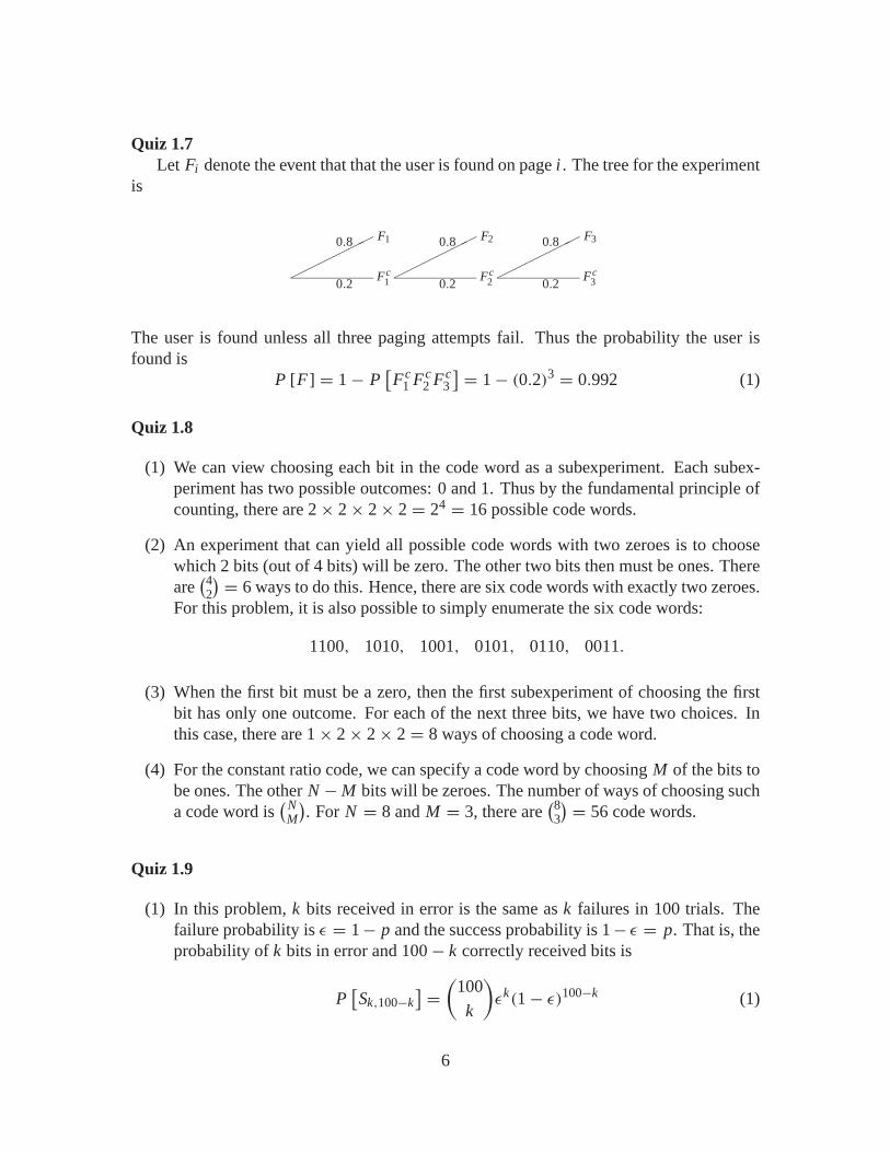
Quiz 1.7Let Fi denote the event that that the user is found on page i . The tree for the experiment
is
������ F10.8
Fc10.2
������ F20.8
Fc20.2
������ F30.8
Fc30.2
The user is found unless all three paging attempts fail. Thus the probability the user isfound is
P [F] = 1− P[Fc
1 Fc2 Fc
3
] = 1− (0.2)3 = 0.992 (1)
Quiz 1.8
(1) We can view choosing each bit in the code word as a subexperiment. Each subex-periment has two possible outcomes: 0 and 1. Thus by the fundamental principle ofcounting, there are 2× 2× 2× 2 = 24 = 16 possible code words.
(2) An experiment that can yield all possible code words with two zeroes is to choosewhich 2 bits (out of 4 bits) will be zero. The other two bits then must be ones. Thereare(4
2
) = 6 ways to do this. Hence, there are six code words with exactly two zeroes.For this problem, it is also possible to simply enumerate the six code words:
1100, 1010, 1001, 0101, 0110, 0011.
(3) When the first bit must be a zero, then the first subexperiment of choosing the firstbit has only one outcome. For each of the next three bits, we have two choices. Inthis case, there are 1× 2× 2× 2 = 8 ways of choosing a code word.
(4) For the constant ratio code, we can specify a code word by choosing M of the bits tobe ones. The other N −M bits will be zeroes. The number of ways of choosing sucha code word is
(NM
). For N = 8 and M = 3, there are
(83
) = 56 code words.
Quiz 1.9
(1) In this problem, k bits received in error is the same as k failures in 100 trials. Thefailure probability is ε = 1− p and the success probability is 1− ε = p. That is, theprobability of k bits in error and 100− k correctly received bits is
P[Sk,100−k
] = (100
k
)εk(1− ε)100−k (1)
6
For ε = 0.01,
P[S0,100
] = (1− ε)100 = (0.99)100 = 0.3660 (2)
P[S1,99
] = 100(0.01)(0.99)99 = 0.3700 (3)
P[S2,98
] = 4950(0.01)2(0.99)98 = 0.1849 (4)
P[S3,97
] = 161, 700(0.01)3(0.99)97 = 0.0610 (5)
(2) The probability a packet is decoded correctly is just
P [C] = P[S0,100
]+ P[S1,99
]+ P[S2,98
]+ P[S3,97
] = 0.9819 (6)
Quiz 1.10Since the chip works only if all n transistors work, the transistors in the chip are like
devices in series. The probability that a chip works is P[C] = pn .The module works if either 8 chips work or 9 chips work. Let Ck denote the event that
exactly k chips work. Since transistor failures are independent of each other, chip failuresare also independent. Thus each P[Ck] has the binomial probability
P [C8] =(
9
8
)(P [C])8 (1− P [C])9−8 = 9p8n(1− pn), (1)
P [C9] = (P [C])9 = p9n. (2)
The probability a memory module works is
P [M] = P [C8]+ P [C9] = p8n(9− 8pn) (3)
Quiz 1.11
R=rand(1,100);X=(R<= 0.4) ...
+ (2*(R>0.4).*(R<=0.9)) ...+ (3*(R>0.9));
Y=hist(X,1:3)
For a MATLAB simulation, we first gen-erate a vector R of 100 random numbers.Second, we generate vector X as a func-tion of R to represent the 3 possible out-comes of a flip. That is, X(i)=1 if flip iwas heads, X(i)=2 if flip i was tails, andX(i)=3) is flip i landed on the edge.
To see how this works, we note there are three cases:
• If R(i) <= 0.4, then X(i)=1.
• If 0.4 < R(i) and R(i)<=0.9, then X(i)=2.
• If 0.9 < R(i), then X(i)=3.
These three cases will have probabilities 0.4, 0.5 and 0.1. Lastly, we use the hist functionto count how many occurences of each possible value of X(i).
7
Quiz Solutions – Chapter 2
Quiz 2.1The sample space, probabilities and corresponding grades for the experiment are
Outcome P[·] G
B B 0.36 3.0BC 0.24 2.5C B 0.24 2.5CC 0.16 2
Quiz 2.2
(1) To find c, we recall that the PMF must sum to 1. That is,
3∑n=1
PN (n) = c
(1+ 1
2+ 1
3
)= 1 (1)
This implies c = 6/11. Now that we have found c, the remaining parts are straight-forward.
(2) P[N = 1] = PN (1) = c = 6/11
(3) P[N ≥ 2] = PN (2)+ PN (3) = c/2+ c/3 = 5/11
(4) P[N > 3] =∑∞n=4 PN (n) = 0
Quiz 2.3Decoding each transmitted bit is an independent trial where we call a bit error a “suc-
cess.” Each bit is in error, that is, the trial is a success, with probability p. Now we caninterpret each experiment in the generic context of independent trials.
(1) The random variable X is the number of trials up to and including the first success.Similar to Example 2.11, X has the geometric PMF
PX (x) ={
p(1− p)x−1 x = 1, 2, . . .
0 otherwise(1)
(2) If p = 0.1, then the probability exactly 10 bits are sent is
P [X = 10] = PX (10) = (0.1)(0.9)9 = 0.0387 (2)
8
The probability that at least 10 bits are sent is P[X ≥ 10] = ∑∞x=10 PX (x). Thissum is not too hard to calculate. However, its even easier to observe that X ≥ 10 ifthe first 10 bits are transmitted correctly. That is,
P [X ≥ 10] = P [first 10 bits are correct] = (1− p)10 (3)
For p = 0.1, P[X ≥ 10] = 0.910 = 0.3487.
(3) The random variable Y is the number of successes in 100 independent trials. Just asin Example 2.13, Y has the binomial PMF
PY (y) =(
100
y
)py(1− p)100−y (4)
If p = 0.01, the probability of exactly 2 errors is
P [Y = 2] = PY (2) =(
100
2
)(0.01)2(0.99)98 = 0.1849 (5)
(4) The probability of no more than 2 errors is
P [Y ≤ 2] = PY (0)+ PY (1)+ PY (2) (6)
= (0.99)100 + 100(0.01)(0.99)99 +(
100
2
)(0.01)2(0.99)98 (7)
= 0.9207 (8)
(5) Random variable Z is the number of trials up to and including the third success. ThusZ has the Pascal PMF (see Example 2.15)
PZ (z) =(
z − 1
2
)p3(1− p)z−3 (9)
Note that PZ (z) > 0 for z = 3, 4, 5, . . ..
(6) If p = 0.25, the probability that the third error occurs on bit 12 is
PZ (12) =(
11
2
)(0.25)3(0.75)9 = 0.0645 (10)
Quiz 2.4Each of these probabilities can be read off the CDF FY (y). However, we must keep in
mind that when FY (y) has a discontinuity at y0, FY (y) takes the upper value FY (y+0 ).
(1) P[Y < 1] = FY (1−) = 0
9
(2) P[Y ≤ 1] = FY (1) = 0.6
(3) P[Y > 2] = 1− P[Y ≤ 2] = 1− FY (2) = 1− 0.8 = 0.2
(4) P[Y ≥ 2] = 1− P[Y < 2] = 1− FY (2−) = 1− 0.6 = 0.4
(5) P[Y = 1] = P[Y ≤ 1] − P[Y < 1] = FY (1+)− FY (1−) = 0.6
(6) P[Y = 3] = P[Y ≤ 3] − P[Y < 3] = FY (3+)− FY (3−) = 0.8− 0.8 = 0
Quiz 2.5
(1) With probability 0.7, a call is a voice call and C = 25. Otherwise, with probability0.3, we have a data call and C = 40. This corresponds to the PMF
PC (c) =⎧⎨⎩
0.7 c = 250.3 c = 400 otherwise
(1)
(2) The expected value of C is
E [C] = 25(0.7)+ 40(0.3) = 29.5 cents (2)
Quiz 2.6
(1) As a function of N , the cost T is
T = 25N + 40(3− N ) = 120− 15N (1)
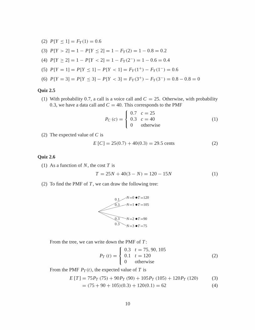
(2) To find the PMF of T , we can draw the following tree:
�������N=00.1
�������N=30.3
�������N=10.3
�������N=20.3
•T=120
•T=105
•T=90
•T=75
From the tree, we can write down the PMF of T :
PT (t) =⎧⎨⎩
0.3 t = 75, 90, 1050.1 t = 1200 otherwise
(2)
From the PMF PT (t), the expected value of T is
E [T ] = 75PT (75)+ 90PT (90)+ 105PT (105)+ 120PT (120) (3)
= (75+ 90+ 105)(0.3)+ 120(0.1) = 62 (4)
10
Quiz 2.7
(1) Using Definition 2.14, the expected number of applications is
E [A] =4∑
a=1
a PA (a) = 1(0.4)+ 2(0.3)+ 3(0.2)+ 4(0.1) = 2 (1)
(2) The number of memory chips is M = g(A) where
g(A) =⎧⎨⎩
4 A = 1, 26 A = 38 A = 4
(2)
(3) By Theorem 2.10, the expected number of memory chips is
E [M] =4∑
a=1
g(A)PA (a) = 4(0.4)+ 4(0.3)+ 6(0.2)+ 8(0.1) = 4.8 (3)
Since E[A] = 2, g(E[A]) = g(2) = 4. However, E[M] = 4.8 �= g(E[A]). The twoquantities are different because g(A) is not of the form αA + β.
Quiz 2.8The PMF PN (n) allows to calculate each of the desired quantities.
(1) The expected value of N is
E [N ] =2∑
n=0
n PN (n) = 0(0.1)+ 1(0.4)+ 2(0.5) = 1.4 (1)
(2) The second moment of N is
E[
N 2]=
2∑n=0
n2 PN (n) = 02(0.1)+ 12(0.4)+ 22(0.5) = 2.4 (2)
(3) The variance of N is
Var[N ] = E[
N 2]− (E [N ])2 = 2.4− (1.4)2 = 0.44 (3)
(4) The standard deviation is σN = √Var[N ] = √0.44 = 0.663.
11
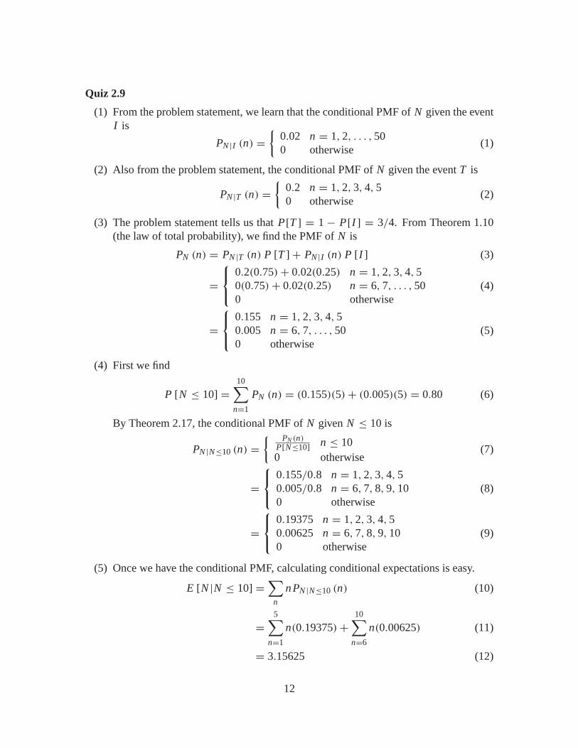
Quiz 2.9
(1) From the problem statement, we learn that the conditional PMF of N given the eventI is
PN |I (n) ={
0.02 n = 1, 2, . . . , 500 otherwise
(1)
(2) Also from the problem statement, the conditional PMF of N given the event T is
PN |T (n) ={
0.2 n = 1, 2, 3, 4, 50 otherwise
(2)
(3) The problem statement tells us that P[T ] = 1 − P[I ] = 3/4. From Theorem 1.10(the law of total probability), we find the PMF of N is
PN (n) = PN |T (n) P [T ]+ PN |I (n) P [I ] (3)
=⎧⎨⎩
0.2(0.75)+ 0.02(0.25) n = 1, 2, 3, 4, 50(0.75)+ 0.02(0.25) n = 6, 7, . . . , 500 otherwise
(4)
=⎧⎨⎩
0.155 n = 1, 2, 3, 4, 50.005 n = 6, 7, . . . , 500 otherwise
(5)
(4) First we find
P [N ≤ 10] =10∑
n=1
PN (n) = (0.155)(5)+ (0.005)(5) = 0.80 (6)
By Theorem 2.17, the conditional PMF of N given N ≤ 10 is
PN |N≤10 (n) ={ PN (n)
P[N≤10] n ≤ 100 otherwise
(7)
=⎧⎨⎩
0.155/0.8 n = 1, 2, 3, 4, 50.005/0.8 n = 6, 7, 8, 9, 100 otherwise
(8)
=⎧⎨⎩
0.19375 n = 1, 2, 3, 4, 50.00625 n = 6, 7, 8, 9, 100 otherwise
(9)
(5) Once we have the conditional PMF, calculating conditional expectations is easy.
E [N |N ≤ 10] =∑
n
n PN |N≤10 (n) (10)
=5∑
n=1
n(0.19375)+10∑
n=6
n(0.00625) (11)
= 3.15625 (12)
12
0 50 1000
2
4
6
8
10
0 500 10000
2
4
6
8
10
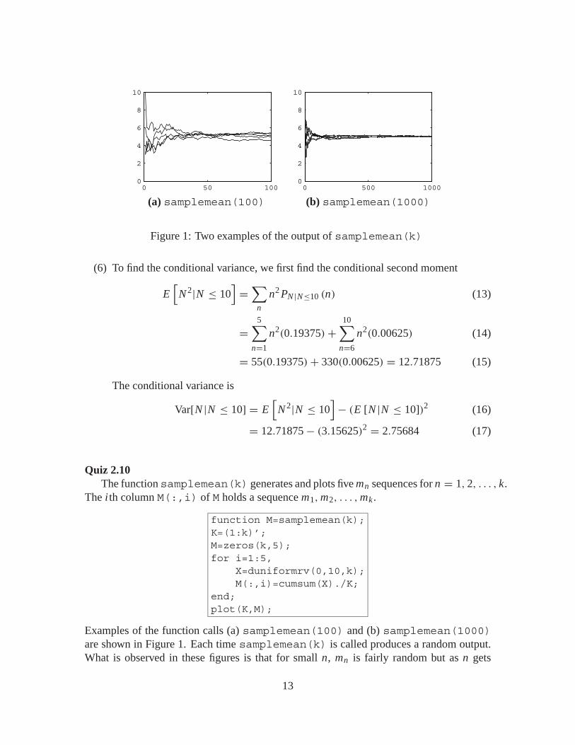
(a) samplemean(100) (b) samplemean(1000)
Figure 1: Two examples of the output of samplemean(k)
(6) To find the conditional variance, we first find the conditional second moment
E[
N 2|N ≤ 10]=∑
n
n2 PN |N≤10 (n) (13)
=5∑
n=1
n2(0.19375)+10∑
n=6
n2(0.00625) (14)
= 55(0.19375)+ 330(0.00625) = 12.71875 (15)
The conditional variance is
Var[N |N ≤ 10] = E[
N 2|N ≤ 10]− (E [N |N ≤ 10])2 (16)
= 12.71875− (3.15625)2 = 2.75684 (17)
Quiz 2.10The function samplemean(k) generates and plots five mn sequences for n = 1, 2, . . . , k.
The i th column M(:,i) of M holds a sequence m1, m2, . . . , mk .
function M=samplemean(k);K=(1:k)’;M=zeros(k,5);for i=1:5,
X=duniformrv(0,10,k);M(:,i)=cumsum(X)./K;
end;plot(K,M);
Examples of the function calls (a) samplemean(100) and (b) samplemean(1000)are shown in Figure 1. Each time samplemean(k) is called produces a random output.What is observed in these figures is that for small n, mn is fairly random but as n gets
13

large, mn gets close to E[X ] = 5. Although each sequence m1, m2, . . . that we generate israndom, the sequences always converges to E[X ]. This random convergence is analyzedin Chapter 7.
14
Quiz Solutions – Chapter 3
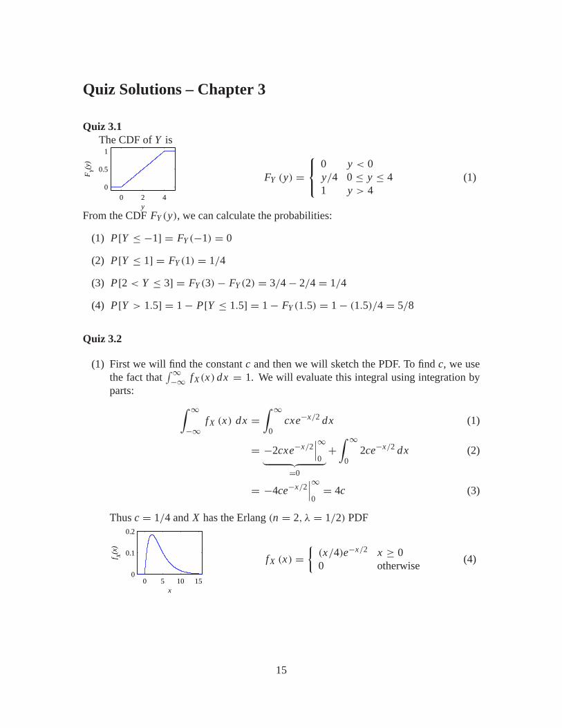
Quiz 3.1The CDF of Y is
0 2 4
0
0.5
1
y
FY(y
)
FY (y) =⎧⎨⎩
0 y < 0y/4 0 ≤ y ≤ 41 y > 4
(1)
From the CDF FY (y), we can calculate the probabilities:
(1) P[Y ≤ −1] = FY (−1) = 0
(2) P[Y ≤ 1] = FY (1) = 1/4
(3) P[2 < Y ≤ 3] = FY (3)− FY (2) = 3/4− 2/4 = 1/4
(4) P[Y > 1.5] = 1− P[Y ≤ 1.5] = 1− FY (1.5) = 1− (1.5)/4 = 5/8
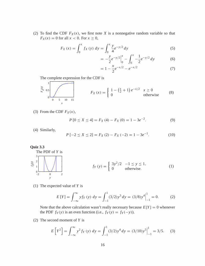
Quiz 3.2
(1) First we will find the constant c and then we will sketch the PDF. To find c, we usethe fact that
∫∞−∞ fX (x) dx = 1. We will evaluate this integral using integration by
parts: ∫ ∞−∞
fX (x) dx =∫ ∞
0cxe−x/2 dx (1)
= −2cxe−x/2∣∣∣∞0︸ ︷︷ ︸
=0
+∫ ∞
02ce−x/2 dx (2)
= −4ce−x/2∣∣∣∞0= 4c (3)
Thus c = 1/4 and X has the Erlang (n = 2, λ = 1/2) PDF
0 5 10 150
0.1
0.2
x
f X(x
)
f X (x) ={
(x/4)e−x/2 x ≥ 00 otherwise
(4)
15
(2) To find the CDF FX (x), we first note X is a nonnegative random variable so thatFX (x) = 0 for all x < 0. For x ≥ 0,
FX (x) =∫ x
0fX (y) dy =
∫ x
0
y
4e−y/2 dy (5)
= − y
2e−y/2
∣∣∣x0−∫ x
0−1
2e−y/2 dy (6)
= 1− x
2e−x/2 − e−x/2 (7)
The complete expression for the CDF is
0 5 10 150
0.5
1
x
FX(x
)
FX (x) ={
1− ( x2 + 1
)e−x/2 x ≥ 0
0 otherwise(8)
(3) From the CDF FX (x),
P [0 ≤ X ≤ 4] = FX (4)− FX (0) = 1− 3e−2. (9)
(4) Similarly,P [−2 ≤ X ≤ 2] = FX (2)− FX (−2) = 1− 3e−1. (10)
Quiz 3.3The PDF of Y is
−2 0 20
1
2
3
y
f Y(y
)
fY (y) ={
3y2/2 −1 ≤ y ≤ 1,
0 otherwise.(1)
(1) The expected value of Y is
E [Y ] =∫ ∞−∞
y fY (y) dy =∫ 1
−1(3/2)y3 dy = (3/8)y4
∣∣∣1−1= 0. (2)
Note that the above calculation wasn’t really necessary because E[Y ] = 0 wheneverthe PDF fY (y) is an even function (i.e., fY (y) = fY (−y)).
(2) The second moment of Y is
E[Y 2]=∫ ∞−∞
y2 fY (y) dy =∫ 1
−1(3/2)y4 dy = (3/10)y5
∣∣∣1−1= 3/5. (3)
16
(3) The variance of Y is
Var[Y ] = E[Y 2]− (E [Y ])2 = 3/5. (4)
(4) The standard deviation of Y is σY = √Var[Y ] = √3/5.
Quiz 3.4
(1) When X is an exponential (λ) random variable, E[X ] = 1/λ and Var[X ] = 1/λ2.Since E[X ] = 3 and Var[X ] = 9, we must have λ = 1/3. The PDF of X is
fX (x) ={
(1/3)e−x/3 x ≥ 0,
0 otherwise.(1)
(2) We know X is a uniform (a, b) random variable. To find a and b, we apply Theo-rem 3.6 to write
E [X ] = a + b
2= 3 Var[X ] = (b − a)2
12= 9. (2)
This impliesa + b = 6, b − a = ±6
√3. (3)
The only valid solution with a < b is
a = 3− 3√
3, b = 3+ 3√
3. (4)
The complete expression for the PDF of X is
fX (x) ={
1/(6√
3) 3− 3√
3 ≤ x < 3+ 3√
3,
0 otherwise.(5)
Quiz 3.5Each of the requested probabilities can be calculated using �(z) function and Table 3.1
or Q(z) and Table 3.2. We start with the sketches.
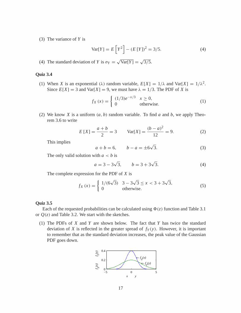
(1) The PDFs of X and Y are shown below. The fact that Y has twice the standarddeviation of X is reflected in the greater spread of fY (y). However, it is importantto remember that as the standard deviation increases, the peak value of the GaussianPDF goes down.
−5 0 50
0.2
0.4
x y
f X(x
)
f
Y(y
)
← fX(x)
← fY(y)
17
(2) Since X is Gaussian (0, 1),
P [−1 < X ≤ 1] = FX (1)− FX (−1) (1)
= �(1)−�(−1) = 2�(1)− 1 = 0.6826. (2)
(3) Since Y is Gaussian (0, 2),
P [−1 < Y ≤ 1] = FY (1)− FY (−1) (3)
= �
(1
σY
)−�
(−1
σY
)= 2�
(1
2
)− 1 = 0.383. (4)
(4) Again, since X is Gaussian (0, 1), P[X > 3.5] = Q(3.5) = 2.33× 10⁻⁴.
(5) Since Y is Gaussian (0, 2), P[Y > 3.5] = Q(3.52 ) = Q(1.75) = 1 − �(1.75) =
0.0401.
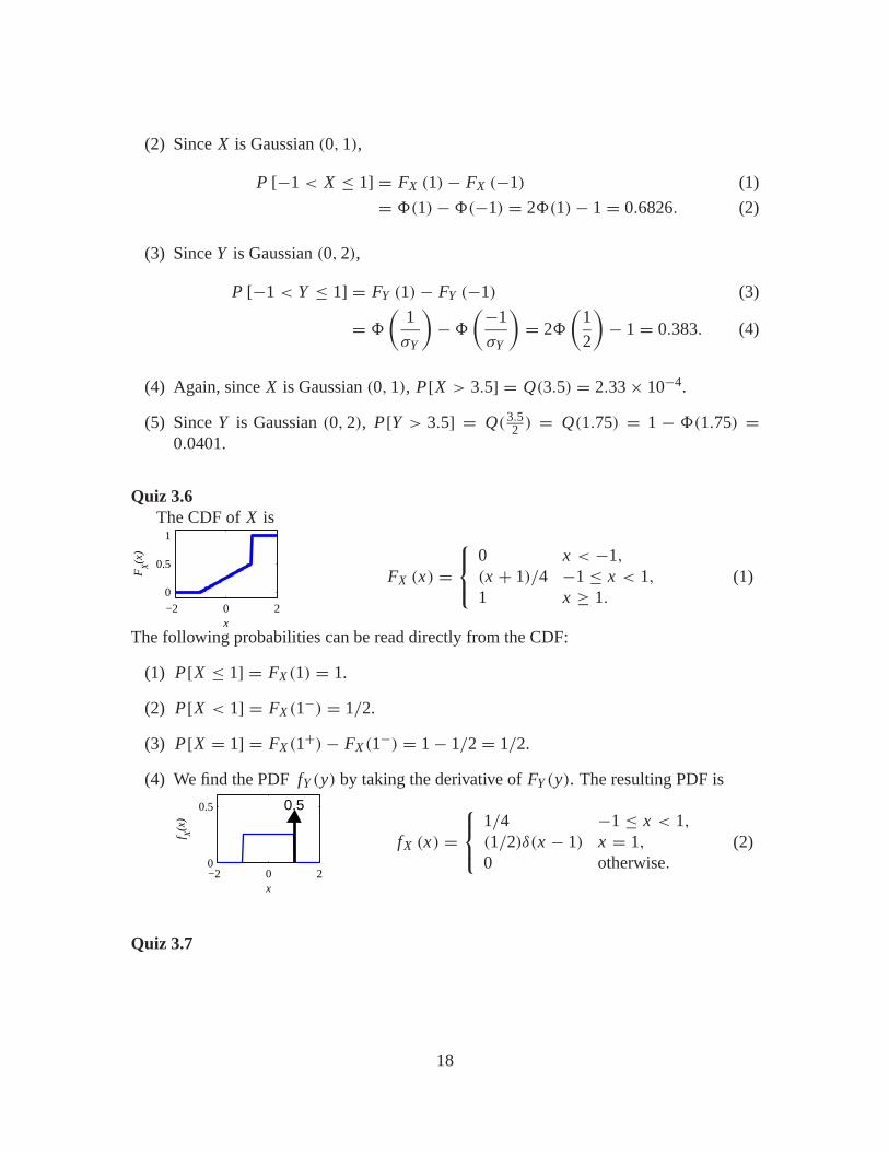
Quiz 3.6The CDF of X is
−2 0 2
0
0.5
1
x
FX(x
)
FX (x) =⎧⎨⎩
0 x < −1,
(x + 1)/4 −1 ≤ x < 1,
1 x ≥ 1.
(1)
The following probabilities can be read directly from the CDF:
(1) P[X ≤ 1] = FX (1) = 1.
(2) P[X < 1] = FX (1−) = 1/2.
(3) P[X = 1] = FX (1+)− FX (1−) = 1− 1/2 = 1/2.
(4) We find the PDF fY (y) by taking the derivative of FY (y). The resulting PDF is
−2 0 20
0.5
x
f X(x
)
0.5
fX (x) =⎧⎨⎩
1/4 −1 ≤ x < 1,
(1/2)δ(x − 1) x = 1,
0 otherwise.(2)
Quiz 3.7
18
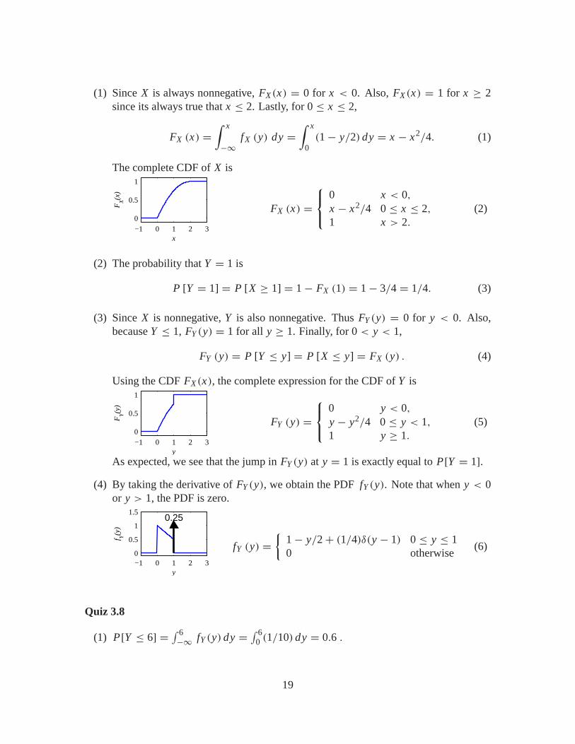
(1) Since X is always nonnegative, FX (x) = 0 for x < 0. Also, FX (x) = 1 for x ≥ 2since its always true that x ≤ 2. Lastly, for 0 ≤ x ≤ 2,
FX (x) =∫ x
−∞fX (y) dy =
∫ x
0(1− y/2) dy = x − x2/4. (1)
The complete CDF of X is
−1 0 1 2 30
0.5
1
x
FX(x
)
FX (x) =⎧⎨⎩
0 x < 0,
x − x2/4 0 ≤ x ≤ 2,
1 x > 2.
(2)
(2) The probability that Y = 1 is
P [Y = 1] = P [X ≥ 1] = 1− FX (1) = 1− 3/4 = 1/4. (3)
(3) Since X is nonnegative, Y is also nonnegative. Thus FY (y) = 0 for y < 0. Also,because Y ≤ 1, FY (y) = 1 for all y ≥ 1. Finally, for 0 < y < 1,
FY (y) = P [Y ≤ y] = P [X ≤ y] = FX (y) . (4)
Using the CDF FX (x), the complete expression for the CDF of Y is
−1 0 1 2 30
0.5
1
y
FY(y
)
FY (y) =⎧⎨⎩
0 y < 0,
y − y2/4 0 ≤ y < 1,
1 y ≥ 1.
(5)
As expected, we see that the jump in FY (y) at y = 1 is exactly equal to P[Y = 1].(4) By taking the derivative of FY (y), we obtain the PDF fY (y). Note that when y < 0
or y > 1, the PDF is zero.
−1 0 1 2 30
0.5
1
1.5
y
f Y(y
)
0.25
fY (y) ={
1− y/2+ (1/4)δ(y − 1) 0 ≤ y ≤ 10 otherwise
(6)
Quiz 3.8
(1) P[Y ≤ 6] = ∫ 6−∞ fY (y) dy = ∫ 6
0 (1/10) dy = 0.6 .
19
(2) From Definition 3.15, the conditional PDF of Y given Y ≤ 6 is
fY |Y≤6 (y) ={
fY (y)P[Y≤6] y ≤ 6,
0 otherwise,={
1/6 0 ≤ y ≤ 6,
0 otherwise.(1)
(3) The probability Y > 8 is
P [Y > 8] =∫ 10
8
1
10dy = 0.2 . (2)
(4) From Definition 3.15, the conditional PDF of Y given Y > 8 is
fY |Y>8 (y) ={
fY (y)P[Y>8] y > 8,
0 otherwise,={
1/2 8 < y ≤ 10,
0 otherwise.(3)
(5) From the conditional PDF fY |Y≤6(y), we can calculate the conditional expectation
E [Y |Y ≤ 6] =∫ ∞−∞
y fY |Y≤6 (y) dy =∫ 6
0
y
6dy = 3. (4)
(6) From the conditional PDF fY |Y>8(y), we can calculate the conditional expectation
E [Y |Y > 8] =∫ ∞−∞
y fY |Y>8 (y) dy =∫ 10
8
y
2dy = 9. (5)
Quiz 3.9A natural way to produce random variables with PDF fT |T >2(t) is to generate samples
of T with PDF fT (t) and then to discard those samples which fail to satisfy the conditionT > 2. Here is a MATLAB function that uses this method:
function t=t2rv(m)i=0;lambda=1/3;t=zeros(m,1);while (i<m),
x=exponentialrv(lambda,1);if (x>2)
t(i+1)=x;i=i+1;
endend
A second method exploits the fact that if T is an exponential (λ) random variable, thenT ′ = T + 2 has PDF fT ′(t) = fT |T >2(t). In this case the command
t=2.0+exponentialrv(1/3,m)
generates the vector t.
20
Quiz Solutions – Chapter 4
Quiz 4.1Each value of the joint CDF can be found by considering the corresponding probability.
(1) FX,Y (−∞, 2) = P[X ≤ −∞, Y ≤ 2] ≤ P[X ≤ −∞] = 0 since X cannot take onthe value −∞.
(2) FX,Y (∞,∞) = P[X ≤ ∞, Y ≤ ∞] = 1. This result is given in Theorem 4.1.
(3) FX,Y (∞, y) = P[X ≤ ∞, Y ≤ y] = P[Y ≤ y] = FY (y).
(4) FX,Y (∞,−∞) = P[X ≤ ∞, Y ≤ −∞] = 0 since Y cannot take on the value −∞.
Quiz 4.2From the joint PMF of Q and G given in the table, we can calculate the requested
probabilities by summing the PMF over those values of Q and G that correspond to theevent.
(1) The probability that Q = 0 is
P [Q = 0] = PQ,G (0, 0)+ PQ,G (0, 1)+ PQ,G (0, 2)+ PQ,G (0, 3) (1)
= 0.06+ 0.18+ 0.24+ 0.12 = 0.6 (2)
(2) The probability that Q = G is
P [Q = G] = PQ,G (0, 0)+ PQ,G (1, 1) = 0.18 (3)
(3) The probability that G > 1 is
P [G > 1] =3∑
g=2
1∑q=0
PQ,G (q, g) (4)
= 0.24+ 0.16+ 0.12+ 0.08 = 0.6 (5)
(4) The probability that G > Q is
P [G > Q] =1∑
q=0
3∑g=q+1
PQ,G (q, g) (6)
= 0.18+ 0.24+ 0.12+ 0.16+ 0.08 = 0.78 (7)
21
Quiz 4.3By Theorem 4.3, the marginal PMF of H is
PH (h) =∑
b=0,2,4
PH,B (h, b) (1)
For each value of h, this corresponds to calculating the row sum across the table of the jointPMF. Similarly, the marginal PMF of B is
PB (b) =1∑
h=−1
PH,B (h, b) (2)
For each value of b, this corresponds to the column sum down the table of the joint PMF.The easiest way to calculate these marginal PMFs is to simply sum each row and column:
PH,B (h, b) b = 0 b = 2 b = 4 PH (h)
h = −1 0 0.4 0.2 0.6h = 0 0.1 0 0.1 0.2h = 1 0.1 0.1 0 0.2PB (b) 0.2 0.5 0.3
(3)
Quiz 4.4To find the constant c, we apply
∫∞−∞∫∞−∞ fX,Y (x, y) dx dy = 1. Specifically,∫ ∞
−∞
∫ ∞−∞
fX,Y (x, y) dx dy =∫ 2
0
∫ 1
0cxy dx dy (1)
= c∫ 2
0y
(x2/2
∣∣∣10
)dy (2)
= (c/2)
∫ 2
0y dy = (c/4)y2
∣∣∣20= c (3)
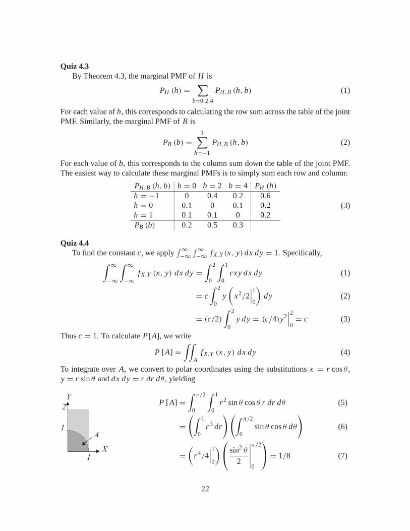
Thus c = 1. To calculate P[A], we write
P [A] =∫∫
AfX,Y (x, y) dx dy (4)
To integrate over A, we convert to polar coordinates using the substitutions x = r cos θ ,y = r sin θ and dx dy = r dr dθ , yielding
Y
X1
1
2
A
P [A] =∫ π/2
0
∫ 1
0r2 sin θ cos θ r dr dθ (5)
=(∫ 1
0r3 dr
)(∫ π/2
0sin θ cos θ dθ
)(6)
=(
r4/4∣∣∣10
)⎛⎝ sin2 θ
2
∣∣∣∣∣π/2
0
⎞⎠ = 1/8 (7)
22
Quiz 4.5By Theorem 4.8, the marginal PDF of X is
fX (x) =∫ ∞−∞
fX,Y (x, y) dy (1)
For x < 0 or x > 1, fX (x) = 0. For 0 ≤ x ≤ 1,
fX (x) = 6
5
∫ 1
0(x + y2) dy = 6
5
(xy + y3/3
)∣∣∣y=1
y=0= 6
5(x + 1/3) = 6x + 2
5(2)
The complete expression for the PDf of X is
fX (x) ={
(6x + 2)/5 0 ≤ x ≤ 10 otherwise
(3)
By the same method we obtain the marginal PDF for Y . For 0 ≤ y ≤ 1,
fY (y) =∫ ∞−∞
fX,Y (x, y) dy (4)
= 6
5
∫ 1
0(x + y2) dx = 6
5
(x2/2+ xy2
)∣∣∣x=1
x=0= 6
5(1/2+ y2) = 3+ 6y2
5(5)
Since fY (y) = 0 for y < 0 or y > 1, the complete expression for the PDF of Y is
fY (y) ={
(3+ 6y2)/5 0 ≤ y ≤ 10 otherwise
(6)
Quiz 4.6
(A) The time required for the transfer is T = L/B. For each pair of values of L and B,we can calculate the time T needed for the transfer. We can write these down on thetable for the joint PMF of L and B as follows:
PL ,B(l, b) b = 14, 400 b = 21, 600 b = 28, 800l = 518, 400 0.20 (T=36) 0.10 (T=24) 0.05 (T=18)
l = 2, 592, 000 0.05 (T=180) 0.10 (T=120) 0.20 (T=90)
l = 7, 776, 000 0.00 (T=540) 0.10 (T=360) 0.20 (T=270)
From the table, writing down the PMF of T is straightforward.
PT (t) =
⎧⎪⎪⎪⎪⎪⎪⎪⎪⎪⎪⎨⎪⎪⎪⎪⎪⎪⎪⎪⎪⎪⎩
0.05 t = 180.1 t = 240.2 t = 36, 900.1 t = 1200.05 t = 1800.2 t = 2700.1 t = 3600 otherwise
(1)
23
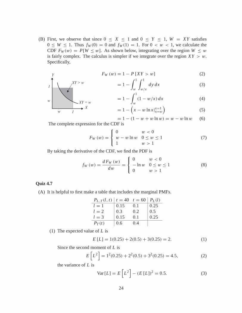
(B) First, we observe that since 0 ≤ X ≤ 1 and 0 ≤ Y ≤ 1, W = XY satisfies0 ≤ W ≤ 1. Thus fW (0) = 0 and fW (1) = 1. For 0 < w < 1, we calculate theCDF FW (w) = P[W ≤ w]. As shown below, integrating over the region W ≤ w
is fairly complex. The calculus is simpler if we integrate over the region XY > w.Specifically,
Y
X1
1XY > w
w
w XY = w
FW (w) = 1− P [XY > w] (2)
= 1−∫ 1
w
∫ 1
w/xdy dx (3)
= 1−∫ 1
w
(1− w/x) dx (4)
= 1−(
x − w ln x |x=1x=w
)(5)
= 1− (1− w + w ln w) = w − w ln w (6)The complete expression for the CDF is
FW (w) =⎧⎨⎩
0 w < 0w − w ln w 0 ≤ w ≤ 11 w > 1
(7)
By taking the derivative of the CDF, we find the PDF is
fW (w) = d FW (w)
dw=⎧⎨⎩
0 w < 0− ln w 0 ≤ w ≤ 10 w > 1
(8)
Quiz 4.7
(A) It is helpful to first make a table that includes the marginal PMFs.
PL ,T (l, t) t = 40 t = 60 PL(l)l = 1 0.15 0.1 0.25l = 2 0.3 0.2 0.5l = 3 0.15 0.1 0.25PT (t) 0.6 0.4
(1) The expected value of L is
E [L] = 1(0.25)+ 2(0.5)+ 3(0.25) = 2. (1)
Since the second moment of L is
E[
L2]= 12(0.25)+ 22(0.5)+ 32(0.25) = 4.5, (2)
the variance of L is
Var [L] = E[
L2]− (E [L])2 = 0.5. (3)
24
(2) The expected value of T is
E [T ] = 40(0.6)+ 60(0.4) = 48. (4)
The second moment of T is
E[T 2]= 402(0.6)+ 602(0.4) = 2400. (5)
ThusVar[T ] = E
[T 2]− (E [T ])2 = 2400− 482 = 96. (6)
(3) The correlation is
E [LT ] =∑
t=40,60
3∑l=1
lt PLT (lt) (7)
= 1(40)(0.15)+ 2(40)(0.3)+ 3(40)(0.15) (8)
+ 1(60)(0.1)+ 2(60)(0.2)+ 3(60)(0.1) (9)
= 96 (10)
(4) From Theorem 4.16(a), the covariance of L and T is
Cov [L , T ] = E [LT ]− E [L] E [T ] = 96− 2(48) = 0 (11)
(5) Since Cov[L , T ] = 0, the correlation coefficient is ρL ,T = 0.
(B) As in the discrete case, the calculations become easier if we first calculate the marginalPDFs fX (x) and fY (y). For 0 ≤ x ≤ 1,
fX (x) =∫ ∞−∞
fX,Y (x, y) dy =∫ 2
0xy dy = 1
2xy2∣∣∣∣y=2
y=0= 2x (12)
Similarly, for 0 ≤ y ≤ 2,
fY (y) =∫ ∞−∞
fX,Y (x, y) dx =∫ 2
0xy dx = 1
2x2y
∣∣∣∣x=1
x=0= y
2(13)
The complete expressions for the marginal PDFs are
fX (x) ={
2x 0 ≤ x ≤ 10 otherwise
fY (y) ={
y/2 0 ≤ y ≤ 20 otherwise
(14)
From the marginal PDFs, it is straightforward to calculate the various expectations.
25
(1) The first and second moments of X are
E [X ] =∫ ∞−∞
x fX (x) dx =∫ 1
02x2 dx = 2
3(15)
E[
X2]=∫ ∞−∞
x2 fX (x) dx =∫ 1
02x3 dx = 1
2(16)
(17)
The variance of X is Var[X ] = E[X2] − (E[X ])2 = 1/18.
(2) The first and second moments of Y are
E [Y ] =∫ ∞−∞
y fY (y) dy =∫ 2
0
1
2y2 dy = 4
3(18)
E[Y 2]=∫ ∞−∞
y2 fY (y) dy =∫ 2
0
1
2y3 dy = 2 (19)
The variance of Y is Var[Y ] = E[Y 2] − (E[Y ])2 = 2− 16/9 = 2/9.
(3) The correlation of X and Y is
E [XY ] =∫ ∞−∞
∫ ∞−∞
xy fX,Y (x, y) dx, dy (20)
=∫ 1
0
∫ 2
0x2y2 dx, dy = x3
3
∣∣∣∣1
0
y3
3
∣∣∣∣2
0= 8
9(21)
(4) The covariance of X and Y is
Cov [X, Y ] = E [XY ]− E [X ] E [Y ] = 8
9−(
2
3
)(4
3
)= 0. (22)
(5) Since Cov[X, Y ] = 0, the correlation coefficient is ρX,Y = 0.
Quiz 4.8
(A) Since the event V > 80 occurs only for the pairs (L , T ) = (2, 60), (L , T ) = (3, 40)
and (L , T ) = (3, 60),
P [A] = P [V > 80] = PL ,T (2, 60)+ PL ,T (3, 40)+ PL ,T (3, 60) = 0.45 (1)
By Definition 4.9,
PL ,T |A (l, t) ={
PL ,T (l,t)P[A] lt > 80
0 otherwise(2)
26
We can represent this conditional PMF in the following table:
PL ,T |A(l, t) t = 40 t = 60l = 1 0 0l = 2 0 4/9l = 3 1/3 2/9
The conditional expectation of V can be found from the conditional PMF.
E [V |A] =∑
l
∑t
lt PL ,T |A (l, t) (3)
= (2 · 60)4
9+ (3 · 40)
1
3+ (3 · 60)
2
9= 133
1
3(4)
For the conditional variance Var[V |A], we first find the conditional second moment
E[V 2|A
]=∑
l
∑t
(lt)2 PL ,T |A (l, t) (5)
= (2 · 60)2 4
9+ (3 · 40)2 1
3+ (3 · 60)2 2
9= 18, 400 (6)
It follows that
Var [V |A] = E[V 2|A
]− (E [V |A])2 = 622
2
9(7)
(B) For continuous random variables X and Y , we first calculate the probability of theconditioning event.
P [B] =∫∫
BfX,Y (x, y) dx dy =
∫ 60
40
∫ 3
80/y
xy
4000dx dy (8)
=∫ 60
40
y
4000
(x2
2
∣∣∣∣3
80/y
)dy (9)
=∫ 60
40
y
4000
(9
2− 3200
y2
)dy (10)
= 9
8− 4
5ln
3
2≈ 0.801 (11)
The conditional PDF of X and Y is
fX,Y |B (x, y) ={
fX,Y (x, y) /P [B] (x, y) ∈ B0 otherwise
(12)
={
K xy 40 ≤ y ≤ 60, 80/y ≤ x ≤ 30 otherwise
(13)
27
where K = (4000P[B])−1. The conditional expectation of W given event B is
E [W |B] =∫ ∞−∞
∫ ∞−∞
xy fX,Y |B (x, y) dx dy (14)
=∫ 60
40
∫ 3
80/yK x2y2 dx dy (15)
= (K/3)
∫ 60
40y2x3
∣∣∣x=3
x=80/ydy (16)
= (K/3)
∫ 60
40
(27y2 − 803/y
)dy (17)
= (K/3)(
9y3 − 803 ln y)∣∣∣60
40≈ 120.78 (18)
The conditional second moment of K given B is
E[W 2|B
]=∫ ∞−∞
∫ ∞−∞
(xy)2 fX,Y |B (x, y) dx dy (19)
=∫ 60
40
∫ 3
80/yK x3y3 dx dy (20)
= (K/4)
∫ 60
40y3x4
∣∣∣x=3
x=80/ydy (21)
= (K/4)
∫ 60
40
(81y3 − 804/y
)dy (22)
= (K/4)((81/4)y4 − 804 ln y
)∣∣∣60
40≈ 16, 116.10 (23)
It follows that the conditional variance of W given B is
Var [W |B] = E[W 2|B
]− (E [W |B])2 ≈ 1528.30 (24)
Quiz 4.9
(A) (1) The joint PMF of A and B can be found from the marginal and conditionalPMFs via PA,B(a, b) = PB|A(b|a)PA(a). Incorporating the information fromthe given conditional PMFs can be confusing, however. Consequently, we cannote that A has range SA = {0, 2} and B has range SB = {0, 1}. A table of thejoint PMF will include all four possible combinations of A and B. The generalform of the table is
PA,B(a, b) b = 0 b = 1a = 0 PB|A(0|0)PA(0) PB|A(1|0)PA(0)
a = 2 PB|A(0|2)PA(2) PB|A(1|2)PA(2)
28
Substituting values from PB|A(b|a) and PA(a), we have
PA,B(a, b) b = 0 b = 1a = 0 (0.8)(0.4) (0.2)(0.4)
a = 2 (0.5)(0.6) (0.5)(0.6)
orPA,B(a, b) b = 0 b = 1
a = 0 0.32 0.08a = 2 0.3 0.3
(2) Given the conditional PMF PB|A(b|2), it is easy to calculate the conditionalexpectation
E [B|A = 2] =1∑
b=0
bPB|A (b|2) = (0)(0.5)+ (1)(0.5) = 0.5 (1)
(3) From the joint PMF PA,B(a, b), we can calculate the the conditional PMF
PA|B (a|0) = PA,B (a, 0)
PB (0)=⎧⎨⎩
0.32/0.62 a = 00.3/0.62 a = 20 otherwise
(2)
=⎧⎨⎩
16/31 a = 015/31 a = 20 otherwise
(3)
(4) We can calculate the conditional variance Var[A|B = 0] using the conditionalPMF PA|B(a|0). First we calculate the conditional expected value
E [A|B = 0] =∑
a
a PA|B (a|0) = 0(16/31)+ 2(15/31) = 30/31 (4)
The conditional second moment is
E[
A2|B = 0]=∑
a
a2 PA|B (a|0) = 02(16/31)+ 22(15/31) = 60/31 (5)
The conditional variance is then
Var[A|B = 0] = E[
A2|B = 0]− (E [A|B = 0])2 = 960
961(6)
(B) (1) The joint PDF of X and Y is
fX,Y (x, y) = fY |X (y|x) fX (x) ={
6y 0 ≤ y ≤ x, 0 ≤ x ≤ 10 otherwise
(7)
(2) From the given conditional PDF fY |X (y|x),
fY |X (y|1/2) ={
8y 0 ≤ y ≤ 1/20 otherwise
(8)
29
(3) The conditional PDF of Y given X = 1/2 is fX |Y (x |1/2) = fX,Y (x, 1/2)/ fY (1/2).To find fY (1/2), we integrate the joint PDF.
fY (1/2) =∫ ∞−∞
fX,1/2 ( ) dx =∫ 1
1/26(1/2) dx = 3/2 (9)
Thus, for 1/2 ≤ x ≤ 1,
fX |Y (x |1/2) = fX,Y (x, 1/2)
fY (1/2)= 6(1/2)
3/2= 2 (10)
(4) From the pervious part, we see that given Y = 1/2, the conditional PDF of Xis uniform (1/2, 1). Thus, by the definition of the uniform (a, b) PDF,
Var [X |Y = 1/2] = (1− 1/2)2
12= 1
48(11)
Quiz 4.10
(A) (1) For random variables X and Y from Example 4.1, we observe that PY (1) =0.09 and PX (0) = 0.01. However,
PX,Y (0, 1) = 0 �= PX (0) PY (1) (1)
Since we have found a pair x, y such that PX,Y (x, y) �= PX (x)PY (y), we canconclude that X and Y are dependent. Note that whenever PX,Y (x, y) = 0,independence requires that either PX (x) = 0 or PY (y) = 0.
(2) For random variables Q and G from Quiz 4.2, it is not obvious whether theyare independent. Unlike X and Y in part (a), there are no obvious pairs q, gthat fail the independence requirement. In this case, we calculate the marginalPMFs from the table of the joint PMF PQ,G(q, g) in Quiz 4.2.
PQ,G(q, g) g = 0 g = 1 g = 2 g = 3 PQ(q)
q = 0 0.06 0.18 0.24 0.12 0.60q = 1 0.04 0.12 0.16 0.08 0.40PG(g) 0.10 0.30 0.40 0.20
Careful study of the table will verify that PQ,G(q, g) = PQ(q)PG(g) for everypair q, g. Hence Q and G are independent.
(B) (1) Since X1 and X2 are independent,
fX1,X2 (x1, x2) = fX1 (x1) fX2 (x2) (2)
={
(1− x1/2)(1− x2/2) 0 ≤ x1 ≤ 2, 0 ≤ x2 ≤ 20 otherwise
(3)
30
(2) Let FX (x) denote the CDF of both X1 and X2. The CDF of Z = max(X1, X2)
is found by observing that Z ≤ z iff X1 ≤ z and X2 ≤ z. That is,
P [Z ≤ z] = P [X1 ≤ z, X2 ≤ z] (4)
= P [X1 ≤ z] P [X2 ≤ z] = [FX (z)]2 (5)
To complete the problem, we need to find the CDF of each Xi . From the PDFfX (x), the CDF is
FX (x) =∫ x
−∞fX (y) dy =
⎧⎨⎩
0 x < 0x − x2/4 0 ≤ x ≤ 21 x > 2
(6)
Thus for 0 ≤ z ≤ 2,FZ (z) = (z − z2/4)2 (7)
The complete expression for the CDF of Z is
FZ (z) =⎧⎨⎩
0 z < 0(z − z2/4)2 0 ≤ z ≤ 21 z > 1
(8)
Quiz 4.11This problem just requires identifying the various terms in Definition 4.17 and Theo-
rem 4.29. Specifically, from the problem statement, we know that ρ = 1/2,
µ1 = µX = 0, µ2 = µY = 0, (1)
and thatσ1 = σX = 1, σ2 = σY = 1. (2)
(1) Applying these facts to Definition 4.17, we have
fX,Y (x, y) = 1√3π2
e−2(x2−xy+y2)/3. (3)
(2) By Theorem 4.30, the conditional expected value and standard deviation of X givenY = y are
E [X |Y = y] = y/2 σX = σ 21 (1− ρ2) = √3/4. (4)
When Y = y = 2, we see that E[X |Y = 2] = 1 and Var[X |Y = 2] = 3/4. Theconditional PDF of X given Y = 2 is simply the Gaussian PDF
fX |Y (x |2) = 1√3π/2
e−2(x−1)2/3. (5)
31

Quiz 4.12One straightforward method is to follow the approach of Example 4.28. Instead, we use
an alternate approach. First we observe that X has the discrete uniform (1, 4) PMF. Also,given X = x , Y has a discrete uniform (1, x) PMF. That is,
PX (x) ={
1/4 x = 1, 2, 3, 4,
0 otherwise,PY |X (y|x) =
{1/x y = 1, . . . , x0 otherwise
(1)
Given X = x , and an independent uniform (0, 1) random variable U , we can generate asample value of Y with a discrete uniform (1, x) PMF via Y = �xU�. This observationprompts the following program:
function xy=dtrianglerv(m)sx=[1;2;3;4];px=0.25*ones(4,1);x=finiterv(sx,px,m);y=ceil(x.*rand(m,1));xy=[x’;y’];
32
Quiz Solutions – Chapter 5
Quiz 5.1We find P[C] by integrating the joint PDF over the region of interest. Specifically,
P [C] =∫ 1/2
0dy2
∫ y2
0dy1
∫ 1/2
0dy4
∫ y4
04dy3 (1)
= 4
(∫ 1/2
0y2 dy2
)(∫ 1/2
0y4 dy4
)= 1/4. (2)
Quiz 5.2By definition of A, Y1 = X1, Y2 = X2− X1 and Y3 = X3− X2. Since 0 < X1 < X2 <
X3, each Yi must be a strictly positive integer. Thus, for y1, y2, y3 ∈ {1, 2, . . .},PY (y) = P [Y1 = y1, Y2 = y2, Y3 = y3] (1)
= P [X1 = y1, X2 − X1 = y2, X3 − X2 = y3] (2)
= P [X1 = y1, X2 = y2 + y1, X3 = y3 + y2 + y1] (3)
= (1− p)3 py1+y2+y3 (4)
By defining the vector a = [1 1 1]′
, the complete expression for the joint PMF of Y is
PY (y) ={
(1− p)pa′y y1, y2, y3 ∈ {1, 2, . . .}0 otherwise
(5)
Quiz 5.3First we note that each marginal PDF is nonzero only if any subset of the xi obeys the
ordering contraints 0 ≤ x1 ≤ x2 ≤ x3 ≤ 1. Within these constraints, we have
fX1,X2 (x1, x2) =∫ ∞−∞
fX (x) dx3 =∫ 1
x2
6 dx3 = 6(1− x2), (1)
fX2,X3 (x2, x3) =∫ ∞−∞
fX (x) dx1 =∫ x2
06 dx1 = 6x2, (2)
fX1,X3 (x1, x3) =∫ ∞−∞
fX (x) dx2 =∫ x3
x1
6 dx2 = 6(x3 − x1). (3)
In particular, we must keep in mind that fX1,X2(x1, x2) = 0 unless 0 ≤ x1 ≤ x2 ≤ 1,fX2,X3(x2, x3) = 0 unless 0 ≤ x2 ≤ x3 ≤ 1, and that fX1,X3(x1, x3) = 0 unless 0 ≤ x1 ≤
33
x3 ≤ 1. The complete expressions are
fX1,X2 (x1, x2) ={
6(1− x2) 0 ≤ x1 ≤ x2 ≤ 10 otherwise
(4)
fX2,X3 (x2, x3) ={
6x2 0 ≤ x2 ≤ x3 ≤ 10 otherwise
(5)
fX1,X3 (x1, x3) ={
6(x3 − x1) 0 ≤ x1 ≤ x3 ≤ 10 otherwise
(6)
Now we can find the marginal PDFs. When 0 ≤ xi ≤ 1 for each xi ,
fX1 (x1) =∫ ∞−∞
fX1,X2 (x1, x2) dx2 =∫ 1
x1
6(1− x2) dx2 = 3(1− x1)2 (7)
fX2 (x2) =∫ ∞−∞
fX2,X3 (x2, x3) dx3 =∫ 1
x2
6x2 dx3 = 6x2(1− x2) (8)
fX3 (x3) =∫ ∞−∞
fX2,X3 (x2, x3) dx2 =∫ x3
06x2 dx2 = 3x2
3 (9)
The complete expressions are
fX1 (x1) ={
3(1− x1)2 0 ≤ x1 ≤ 1
0 otherwise(10)
fX2 (x2) ={
6x2(1− x2) 0 ≤ x2 ≤ 10 otherwise
(11)
fX3 (x3) ={
3x23 0 ≤ x3 ≤ 1
0 otherwise(12)
Quiz 5.4In the PDF fY(y), the components have dependencies as a result of the ordering con-
straints Y1 ≤ Y2 and Y3 ≤ Y4. We can separate these constraints by creating the vectors
V =[
Y1
Y2
], W =
[Y3
Y4
]. (1)
The joint PDF of V and W is
fV,W (v, w) ={
4 0 ≤ v1 ≤ v2 ≤ 1, 0 ≤ w1 ≤ w2 ≤ 10 otherwise
(2)
34
We must verify that V and W are independent. For 0 ≤ v1 ≤ v2 ≤ 1,
fV (v) =∫∫
fV,W (v, w) dw1 dw2 (3)
=∫ 1
0
(∫ 1
w1
4 dw2
)dw1 (4)
=∫ 1
04(1− w1) dw1 = 2 (5)
Similarly, for 0 ≤ w1 ≤ w2 ≤ 1,
fW (w) =∫∫
fV,W (v, w) dv1 dv2 (6)
=∫ 1
0
(∫ 1
v1
4 dv2
)dv1 = 2 (7)
It follows that V and W have PDFs
fV (v) ={
2 0 ≤ v1 ≤ v2 ≤ 10 otherwise
, fW (w) ={
2 0 ≤ w1 ≤ w2 ≤ 10 otherwise
(8)
It is easy to verify that fV,W(v, w) = fV(v) fW(w), confirming that V and W are indepen-dent vectors.
Quiz 5.5
(A) Referring to Theorem 1.19, each test is a subexperiment with three possible out-comes: L , A and R. In five trials, the vector X = [X1 X2 X3
]′indicating the
number of outcomes of each subexperiment has the multinomial PMF
PX (x) =⎧⎨⎩( 5
x1,x2,x3
)(0.3)x1(0.6)x2(0.1)x3 x1 + x2 + x3 = 5;
x1, x2, x3 ∈ {0, 1, . . . , 5}0 otherwise
(1)
We can find the marginal PMF for each Xi from the joint PMF PX(x); however itis simpler to just start from first principles and observe that X1 is the number ofoccurrences of L in five independent tests. If we view each test as a trial with successprobability P[L] = 0.3, we see that X1 is a binomial (n, p) = (5, 0.3) randomvariable. Similarly, X2 is a binomial (5, 0.6) random variable and X3 is a binomial(5, 0.1) random variable. That is, for p1 = 0.3, p2 = 0.6 and p3 = 0.1,
PXi (x) ={ (5
x
)px
i (1− pi )5−x x = 0, 1, . . . , 5
0 otherwise(2)
35
From the marginal PMFs, we see that X1, X2 and X3 are not independent. Hence, wemust use Theorem 5.6 to find the PMF of W . In particular, since X1 + X2 + X3 = 5and since each Xi is non-negative, PW (0) = PW (1) = 0. Furthermore,
PW (2) = PX (1, 2, 2)+ PX (2, 1, 2)+ PX (2, 2, 1) (3)
= 5![0.3(0.6)2(0.1)2 + 0.32(0.6)(0.1)2 + 0.32(0.6)2(0.1)]2!2!1! (4)
= 0.1458 (5)
In addition, for w = 3, w = 4, and w = 5, the event W = w occurs if and only ifone of the mutually exclusive events X1 = w, X2 = w, or X3 = w occurs. Thus,
PW (3) = PX1 (3)+ PX2 (3)+ PX3 (3) = 0.486 (6)
PW (4) = PX1 (4)+ PX2 (4)+ PX3 (4) = 0.288 (7)
PW (5) = PX1 (5)+ PX2 (5)+ PX3 (5) = 0.0802 (8)
(B) Since each Yi = 2Xi + 4, we can apply Theorem 5.10 to write
fY (y) = 1
23fX
(y1 − 4
2,
y2 − 4
2,
y3 − 4
2
)(9)
={
(1/8)e−(y3−4)/2 4 ≤ y1 ≤ y2 ≤ y3
0 otherwise(10)
Note that for other matrices A, the constraints on y resulting from the constraints0 ≤ X1 ≤ X2 ≤ X3 can be much more complicated.
Quiz 5.6We start by finding the components E[Xi ] =
∫∞−∞ x fXi (x) dx of µX . To do so, we use
the marginal PDFs fXi (x) found in Quiz 5.3:
E [X1] =∫ 1
03x(1− x)2 dx = 1/4, (1)
E [X2] =∫ 1
06x2(1− x) dx = 1/2, (2)
E [X3] =∫ 1
03x3 dx = 3/4. (3)
To find the correlation matrix RX , we need to find E[Xi X j ] for all i and j . We start with
36
the second moments:
E[
X21
]=∫ 1
03x2(1− x)2 dx = 1/10. (4)
E[
X22
]=∫ 1
06x3(1− x) dx = 3/10. (5)
E[
X23
]=∫ 1
03x4 dx = 3/5. (6)
Using marginal PDFs from Quiz 5.3, the cross terms are
E [X1 X2] =∫ ∞−∞
∫ ∞−∞
x1x2 fX1,X2 (x1, x2) , dx1 dx2 (7)
=∫ 1
0
(∫ 1
x1
6x1x2(1− x2) dx2
)dx1 (8)
=∫ 1
0[x1 − 3x3
1 + 2x41 ] dx1 = 3/20. (9)
E [X2 X3] =∫ 1
0
∫ 1
x2
6x22 x3 dx3 dx2 (10)
=∫ 1
0[3x2
2 − 3x42 ] dx2 = 2/5 (11)
E [X1 X3] =∫ 1
0
∫ 1
x1
6x1x3(x3 − x1) dx3 dx1. (12)
=∫ 1
0
((2x1x3
3 − 3x21 x2
3)
∣∣∣x3=1
x3=x1
)dx1 (13)
=∫ 1
0[2x1 − 3x2
1 + x41 ] dx1 = 1/5. (14)
Summarizing the results, X has correlation matrix
RX =⎡⎣1/10 3/20 1/5
3/20 3/10 2/51/5 2/5 3/5
⎤⎦ . (15)
Vector X has covariance matrix
CX = RX − E [X] E [X]′ (16)
=⎡⎣1/10 3/20 1/5
3/20 3/10 2/51/5 2/5 3/5
⎤⎦−
⎡⎣1/4
1/23/4
⎤⎦[1/4 1/2 3/4
](17)
=⎡⎣1/10 3/20 1/5
3/20 3/10 2/51/5 2/5 3/5
⎤⎦−
⎡⎣1/16 1/8 3/16
1/8 1/4 3/83/16 3/8 9/16
⎤⎦ = 1
80
⎡⎣3 2 1
2 4 21 2 3
⎤⎦ . (18)
37
This problem shows that even for fairly simple joint PDFs, computing the covariance matrixby calculus can be a time consuming task.
Quiz 5.7We observe that X = AZ+ b where
A =[
2 11 −1
], b =
[20
]. (1)
It follows from Theorem 5.18 that µX = b and that
CX = AA′ =[
2 11 −1
] [2 11 −1
]=[
5 11 2
]. (2)
Quiz 5.8First, we observe that Y = AT where A = [1/31 1/31 · · · 1/31
]′. Since T is a
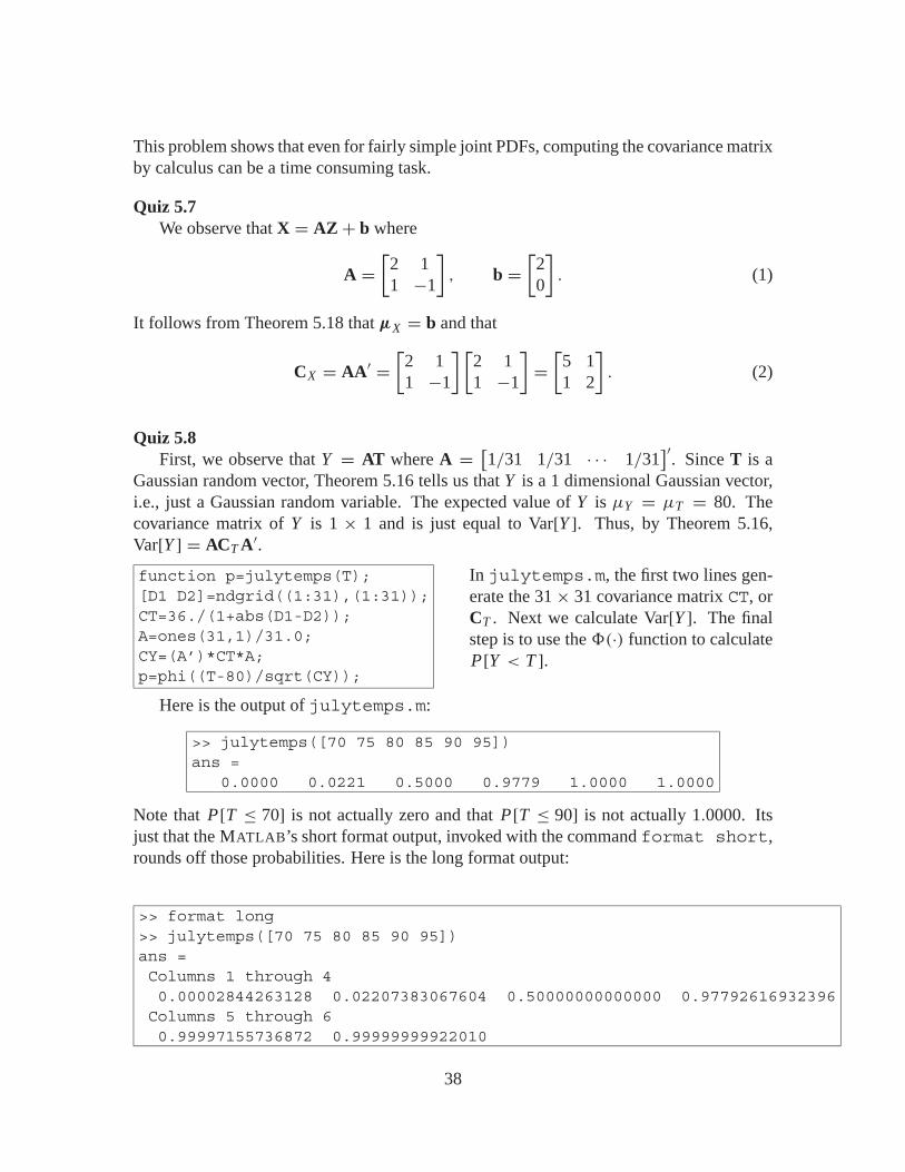
Gaussian random vector, Theorem 5.16 tells us that Y is a 1 dimensional Gaussian vector,i.e., just a Gaussian random variable. The expected value of Y is µY = µT = 80. Thecovariance matrix of Y is 1 × 1 and is just equal to Var[Y ]. Thus, by Theorem 5.16,Var[Y ] = ACT A′.function p=julytemps(T);[D1 D2]=ndgrid((1:31),(1:31));CT=36./(1+abs(D1-D2));A=ones(31,1)/31.0;CY=(A’)*CT*A;p=phi((T-80)/sqrt(CY));
In julytemps.m, the first two lines gen-erate the 31× 31 covariance matrix CT, orCT . Next we calculate Var[Y ]. The finalstep is to use the �(·) function to calculateP[Y < T ].
Here is the output of julytemps.m:
>> julytemps([70 75 80 85 90 95])ans =
0.0000 0.0221 0.5000 0.9779 1.0000 1.0000
Note that P[T ≤ 70] is not actually zero and that P[T ≤ 90] is not actually 1.0000. Itsjust that the MATLAB’s short format output, invoked with the command format short,rounds off those probabilities. Here is the long format output:
>> format long>> julytemps([70 75 80 85 90 95])ans =Columns 1 through 40.00002844263128 0.02207383067604 0.50000000000000 0.97792616932396
Columns 5 through 60.99997155736872 0.99999999922010
38

The ndgrid function is a useful to way calculate many covariance matrices. However, inthis problem, CX has a special structure; the i, j th element is
CT(i, j) = c|i− j | = 36
1+ |i − j | . (1)
If we write out the elements of the covariance matrix, we see that
CT =
⎡⎢⎢⎢⎣
c0 c1 · · · c30
c1 c0. . .
......
. . .. . . c1
c30 · · · c1 c0
⎤⎥⎥⎥⎦ . (2)
This covariance matrix is known as a symmetric Toeplitz matrix. We will see in Chap-ters 9 and 11 that Toeplitz covariance matrices are quite common. In fact, MATLAB has atoeplitz function for generating them. The function julytemps2 use the toeplitzto generate the correlation matrix CT.
function p=julytemps2(T);c=36./(1+abs(0:30));CT=toeplitz(c);A=ones(31,1)/31.0;CY=(A’)*CT*A;p=phi((T-80)/sqrt(CY));
39
Quiz Solutions – Chapter 6
Quiz 6.1Let K1, . . . , Kn denote a sequence of iid random variables each with PMF
PK (k) ={
1/4 k = 1, . . . , 40 otherwise
(1)
We can write Wn in the form of Wn = K1 + · · · + Kn . First, we note that the first twomoments of Ki are
E [Ki ] = (1+ 2+ 3+ 4)/4 = 2.5 (2)
E[
K 2i
]= (12 + 22 + 32 + 42)/4 = 7.5 (3)
Thus the variance of Ki is
Var[Ki ] = E[
K 2i
]− (E [Ki ])
2 = 7.5− (2.5)2 = 1.25 (4)
Since E[Ki ] = 2.5, the expected value of Wn is
E [Wn] = E [K1]+ · · · + E [Kn] = nE [Ki ] = 2.5n (5)
Since the rolls are independent, the random variables K1, . . . , Kn are independent. Hence,by Theorem 6.3, the variance of the sum equals the sum of the variances. That is,
Var[Wn] = Var[K1] + · · · + Var[Kn] = 1.25n (6)
Quiz 6.2Random variables X and Y have PDFs
fX (x) ={
3e−3x x ≥ 00 otherwise
fY (y) ={
2e−2y y ≥ 00 otherwise
(1)
Since X and Y are nonnegative, W = X + Y is nonnegative. By Theorem 6.5, the PDF ofW = X + Y is
fW (w) =∫ ∞−∞
fX (w − y) fY (y) dy = 6∫ w
0e−3(w−y)e−2y dy (2)
Fortunately, this integral is easy to evaluate. For w > 0,
fW (w) = e−3w ey∣∣w0 = 6
(e−2w − e−3w
)(3)
Since fW (w) = 0 for w < 0, a conmplete expression for the PDF of W is
fW (w) ={
6e−2w(1− e−w
)w ≥ 0,
0 otherwise.(4)
40
Quiz 6.3The MGF of K is
φK (s) = E[esK ] == 4∑
k=0
(0.2)esk = 0.2(
1+ es + e2s + e3s + e4s)
(1)
We find the moments by taking derivatives. The first derivative of φK (s) is
dφK (s)
ds= 0.2(es + 2e2s + 3e3s + 4e4s) (2)
Evaluating the derivative at s = 0 yields
E [K ] = dφK (s)
ds
∣∣∣∣s=0= 0.2(1+ 2+ 3+ 4) = 2 (3)
To find higher-order moments, we continue to take derivatives:
E[
K 2]= d2φK (s)
ds2
∣∣∣∣s=0= 0.2(es + 4e2s + 9e3s + 16e4s)
∣∣∣s=0= 6 (4)
E[
K 3]= d3φK (s)
ds3
∣∣∣∣s=0= 0.2(es + 8e2s + 27e3s + 64e4s)
∣∣∣s=0= 20 (5)
E[
K 4]= d4φK (s)
ds4
∣∣∣∣s=0= 0.2(es + 16e2s + 81e3s + 256e4s)
∣∣∣s=0= 70.8 (6)
(7)
Quiz 6.4
(A) Each Ki has MGF
φK (s) = E[esKi
] = es + e2s + · · · + ens
n= es(1− ens)
n(1− es)(1)
Since the sequence of Ki is independent, Theorem 6.8 says the MGF of J is
φJ (s) = (φK (s))m = ems(1− ens)m
nm(1− es)m(2)
(B) Since the set of α j X j are independent Gaussian random variables, Theorem 6.10says that W is a Gaussian random variable. Thus to find the PDF of W , we needonly find the expected value and variance. Since the expectation of the sum equalsthe sum of the expectations:
E [W ] = αE [X1]+ α2 E [X2]+ · · · + αn E [Xn] = 0 (3)
41
Since the α j X j are independent, the variance of the sum equals the sum of the vari-ances:
Var[W ] = α2 Var[X1] + α4 Var[X2] + · · · + α2n Var[Xn] (4)
= α2 + 2(α2)2 + 3(α2)3 + · · · + n(α2)n (5)
Defining q = α2, we can use Math Fact B.6 to write
Var[W ] = α2 − α2n+2[1+ n(1− α2)](1− α2)2
(6)
With E[W ] = 0 and σ 2W = Var[W ], we can write the PDF of W as
fW (w) = 1√2πσ 2
W
e−w2/2σ 2W (7)
Quiz 6.5
(1) From Table 6.1, each Xi has MGF φX (s) and random variable N has MGF φN (s)where
φX (s) = 1
1− s, φN (s) =
15es
1− 45es
. (1)
From Theorem 6.12, R has MGF
φR(s) = φN (ln φX (s)) =15φX (s)
1− 45φX (s)
(2)
Substituting the expression for φX (s) yields
φR(s) =15
15 − s
. (3)
(2) From Table 6.1, we see that R has the MGF of an exponential (1/5) random variable.The corresponding PDF is
fR (r) ={
(1/5)e−r/5 r ≥ 00 otherwise
(4)
This quiz is an example of the general result that a geometric sum of exponentialrandom variables is an exponential random variable.
42
Quiz 6.6
(1) The expected access time is
E [X ] =∫ ∞−∞
x fX (x) dx =∫ 12
0
x
12dx = 6 msec (1)
(2) The second moment of the access time is
E[
X2]=∫ ∞−∞
x2 fX (x) dx =∫ 12
0
x2
12dx = 48 (2)
The variance of the access time is Var[X ] = E[X2] − (E[X ])2 = 48− 36 = 12.
(3) Using Xi to denote the access time of block i , we can write
A = X1 + X2 + · · · + X12 (3)
Since the expectation of the sum equals the sum of the expectations,
E [A] = E [X1]+ · · · + E [X12] = 12E [X ] = 72 msec (4)
(4) Since the Xi are independent,
Var[A] = Var[X1] + · · · + Var[X12] = 12 Var[X ] = 144 (5)
Hence, the standard deviation of A is σA = 12
(5) To use the central limit theorem, we write
P [A > 75] = 1− P [A ≤ 75] (6)
= 1− P
[A − E [A]
σA≤ 75− E [A]
σA
](7)
≈ 1−�
(75− 72
12
)(8)
= 1− 0.5987 = 0.4013 (9)
Note that we used Table 3.1 to look up �(0.25).
(6) Once again, we use the central limit theorem and Table 3.1 to estimate
P [A < 48] = P
[A − E [A]
σA<
48− E [A]
σA
](10)
≈ �
(48− 72
12
)(11)
= 1−�(2) = 1− 0.9773 = 0.0227 (12)
43
Quiz 6.7Random variable Kn has a binomial distribution for n trials and success probability
P[V ] = 3/4.
(1) The expected number of voice calls out of 48 calls is E[K48] = 48P[V ] = 36.
(2) The variance of K48 is
Var[K48] = 48P [V ] (1− P [V ]) = 48(3/4)(1/4) = 9 (1)
Thus K48 has standard deviation σK48 = 3.
(3) Using the ordinary central limit theorem and Table 3.1 yields
P [30 ≤ K48 ≤ 42] ≈ �
(42− 36
3
)−�
(30− 36
3
)= �(2)−�(−2) (2)
Recalling that �(−x) = 1−�(x), we have
P [30 ≤ K48 ≤ 42] ≈ 2�(2)− 1 = 0.9545 (3)
(4) Since K48 is a discrete random variable, we can use the De Moivre-Laplace approx-imation to estimate
P [30 ≤ K48 ≤ 42] ≈ �
(42+ 0.5− 36
3
)−�
(30− 0.5− 36
3
)(4)
= 2�(2.16666)− 1 = 0.9687 (5)
Quiz 6.8The train interarrival times X1, X2, X3 are iid exponential (λ) random variables. The
arrival time of the third train is
W = X1 + X2 + X3. (1)
In Theorem 6.11, we found that the sum of three iid exponential (λ) random variables is anErlang (n = 3, λ) random variable. From Appendix A, we find that W has expected valueand variance
E [W ] = 3/λ = 6 Var[W ] = 3/λ2 = 12 (2)
(1) By the Central Limit Theorem,
P [W > 20] = P
[W − 6√
12>
20− 6√12
]≈ Q(7/
√3) = 2.66× 10⁻⁵ (3)
44
(2) To use the Chernoff bound, we note that the MGF of W is
φW (s) =(
λ
λ− s
)3
= 1
(1− 2s)3(4)
The Chernoff bound states that
P [W > 20] ≤ mins≥0
e−20sφX (s) = mins≥0
e−20s
(1− 2s)3(5)
To minimize h(s) = e−20s/(1− 2s)3, we set the derivative of h(s) to zero:
dh(s)
ds= −20(1− 2s)3e−20s + 6e−20s(1− 2s)2
(1− 2s)6= 0 (6)
This implies 20(1 − 2s) = 6 or s = 7/20. Applying s = 7/20 into the Chernoffbound yields
P [W > 20] ≤ e−20s
(1− 2s)3
∣∣∣∣s=7/20
= (10/3)3e−7 = 0.0338 (7)
(3) Theorem 3.11 says that for any w > 0, the CDF of the Erlang (λ, 3) random variableW satisfies
FW (w) = 1−2∑
k=0
(λw)ke−λw
k! (8)
Equivalently, for λ = 1/2 and w = 20,
P [W > 20] = 1− FW (20) (9)
= e−10(
1+ 10
1! +102
2!)= 61e−10 = 0.0028 (10)
Although the Chernoff bound is relatively weak in that it overestimates the proba-bility by roughly a factor of 12, it is a valid bound. By contrast, the Central LimitTheorem approximation grossly underestimates the true probability.
Quiz 6.9One solution to this problem is to follow the approach of Example 6.19:
%unifbinom100.msx=0:100;sy=0:100;px=binomialpmf(100,0.5,sx); py=duniformpmf(0,100,sy);[SX,SY]=ndgrid(sx,sy); [PX,PY]=ndgrid(px,py);SW=SX+SY; PW=PX.*PY;sw=unique(SW); pw=finitepmf(SW,PW,sw);pmfplot(sw,pw,’\itw’,’\itP_W(w)’);
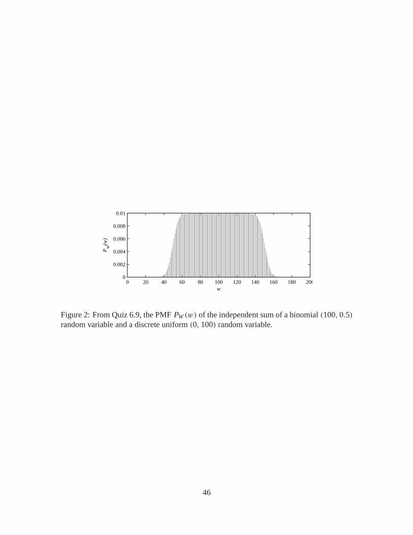
A graph of the PMF PW (w) appears in Figure 2 With some thought, it should be apparentthat the finitepmf function is implementing the convolution of the two PMFs.
45
0 20 40 60 80 100 120 140 160 180 2000
0.002
0.004
0.006
0.008
0.01
w
PW
(w)
Figure 2: From Quiz 6.9, the PMF PW (w) of the independent sum of a binomial (100, 0.5)
random variable and a discrete uniform (0, 100) random variable.
46
Quiz Solutions – Chapter 7
Quiz 7.1An exponential random variable with expected value 1 also has variance 1. By Theo-
rem 7.1, Mn(X) has variance Var[Mn(X)] = 1/n. Hence, we need n = 100 samples.
Quiz 7.2The arrival time of the third elevator is W = X1 + X2 + X3. Since each Xi is uniform
(0, 30),
E [Xi ] = 15, Var [Xi ] = (30− 0)2
12= 75. (1)
Thus E[W ] = 3E[Xi ] = 45, and Var[W ] = 3 Var[Xi ] = 225.
(1) By the Markov inequality,
P [W > 75] ≤ E [W ]
75= 45
75= 3
5(2)
(2) By the Chebyshev inequality,
P [W > 75] = P [W − E [W ] > 30] (3)
≤ P [|W − E [W ]| > 30] ≤ Var [W ]
302= 225
900= 1
4(4)
Quiz 7.3Define the random variable W = (X − µX )2. Observe that V100(X) = M100(W ). By
Theorem 7.6, the mean square error is
E[(M100(W )− µW )2
]= Var[W ]
100(1)
Observe that µX = 0 so that W = X2. Thus,
µW = E[
X2]=∫ 1
−1x2 fX (x) dx = 1/3 (2)
E[W 2]= E
[X4]=∫ 1
−1x4 fX (x) dx = 1/5 (3)
Therefore Var[W ] = E[W 2] − µ2W = 1/5 − (1/3)2 = 4/45 and the mean square error is
4/4500 = 0.000889.
47
Quiz 7.4Assuming the number n of samples is large, we can use a Gaussian approximation for
Mn(X). SinceE[X ] = p and Var[X ] = p(1− p), we apply Theorem 7.13 which says thatthe interval estimate
Mn(X)− c ≤ p ≤ Mn(X)+ c (1)
has confidence coefficient 1− α where
α = 2− 2�
(c√
n
p(1− p)
). (2)
We must ensure for every value of p that 1 − α ≥ 0.9 or α ≤ 0.1. Equivalently, we musthave
�
(c√
n
p(1− p)
)≥ 0.95 (3)
for every value of p. Since �(x) is an increasing function of x , we must satisfy c√
n ≥1.65p(1− p). Since p(1− p) ≤ 1/4 for all p, we require that
c ≥ 1.65
4√
n= 0.41√
n. (4)
The 0.9 confidence interval estimate of p is
Mn(X)− 0.41√n≤ p ≤ Mn(X)+ 0.41√
n. (5)
For the 0.99 confidence interval, we have α ≤ 0.01, implying �(c√
n/(p(1−p))) ≥ 0.995.This implies c
√n ≥ 2.58p(1 − p). Since p(1 − p) ≤ 1/4 for all p, we require that
c ≥ (0.25)(2.58)/√
n. In this case, the 0.99 confidence interval estimate is
Mn(X)− 0.645√n≤ p ≤ Mn(X)+ 0.645√
n. (6)
Note that if M100(X) = 0.4, then the 0.99 confidence interval estimate is
0.3355 ≤ p ≤ 0.4645. (7)
The interval is wide because the 0.99 confidence is high.
Quiz 7.5Following the approach of bernoullitraces.m, we generate m = 1000 sample
paths, each sample path having n = 100 Bernoulli traces. at time k, OK(k) counts thefraction of sample paths that have sample mean within one standard error of p. The pro-gram bernoullisample.m generates graphs the number of traces within one standarderror as a function of the time, i.e. the number of trials in each trace.
48
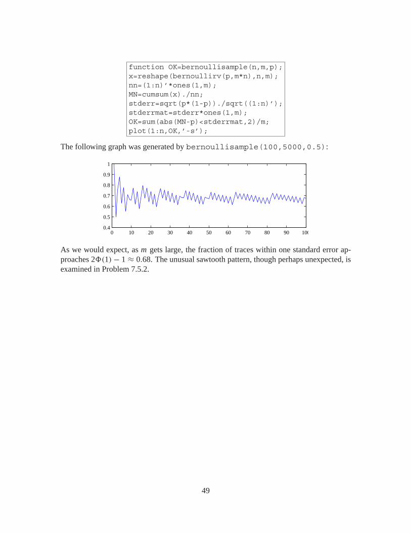
function OK=bernoullisample(n,m,p);x=reshape(bernoullirv(p,m*n),n,m);nn=(1:n)’*ones(1,m);MN=cumsum(x)./nn;stderr=sqrt(p*(1-p))./sqrt((1:n)’);stderrmat=stderr*ones(1,m);OK=sum(abs(MN-p)<stderrmat,2)/m;plot(1:n,OK,’-s’);
The following graph was generated by bernoullisample(100,5000,0.5):
0 10 20 30 40 50 60 70 80 90 1000.4
0.5
0.6
0.7
0.8
0.9
1
As we would expect, as m gets large, the fraction of traces within one standard error ap-proaches 2�(1)− 1 ≈ 0.68. The unusual sawtooth pattern, though perhaps unexpected, isexamined in Problem 7.5.2.
49
Quiz Solutions – Chapter 8
Quiz 8.1From the problem statement, each Xi has PDF and CDF
fXi (x) ={
e−x x ≥ 00 otherwise
FXi (x) ={
0 x < 01− e−x x ≥ 0
(1)
Hence, the CDF of the maximum of X1, . . . , X15 obeys
FX (x) = P [X ≤ x] = P [X1 ≤ x, X2 ≤ x, · · · , X15 ≤ x] = [P [Xi ≤ x]]15 . (2)
This implies that for x ≥ 0,
FX (x) = [FXi (x)]15 = [1− e−x]15
(3)
To design a significance test, we must choose a rejection region for X . A reasonable choiceis to reject the hypothesis if X is too small. That is, let R = {X ≤ r}. For a significancelevel of α = 0.01, we obtain
α = P [X ≤ r ] = (1− e−r )15 = 0.01 (4)
It is straightforward to show that
r = − ln[1− (0.01)1/15
]= 1.33 (5)
Hence, if we observe X < 1.33, then we reject the hypothesis.
Quiz 8.2From the problem statement, the conditional PMFs of K are
PK |H0 (k) ={
104ke−104
k! k = 0, 1, . . .
0 otherwise(1)
PK |H1 (k) ={
106ke−106
k! k = 0, 1, . . .
0 otherwise(2)
Since the two hypotheses are equally likely, the MAP and ML tests are the same. FromTheorem 8.6, the ML hypothesis rule is
k ∈ A0 if PK |H0 (k) ≥ PK |H1 (k) ; k ∈ A1 otherwise. (3)
This rule simplifies to
k ∈ A0 if k ≤ k∗ = 106 − 104
ln 100= 214, 975.7; k ∈ A1 otherwise. (4)
Thus if we observe at least 214, 976 photons, then we accept hypothesis H1.
50
Quiz 8.3For the QPSK system, a symbol error occurs when si is transmitted but (X1, X2) ∈ A j
for some j �= i . For a QPSK system, it is easier to calculate the probability of a correctdecision. Given H0, the conditional probability of a correct decision is
P [C |H0] = P [X1 > 0, X2 > 0|H0] = P[√
E/2+ N1 > 0,√
E/2+ N2 > 0]
(1)
Because of the symmetry of the signals, P[C |H0] = P[C |Hi ] for all i . This implies theprobability of a correct decision is P[C] = P[C |H0]. Since N1 and N2 are iid Gaussian(0, σ ) random variables, we have
P [C] = P [C |H0] = P[√
E/2+ N1 > 0]
P[√
E/2+ N2 > 0]
(2)
=(
P[
N1 > −√E/2])2
(3)
=[
1−�
(−√E/2
σ
)]2
(4)
Since �(−x) = 1 − �(x), we have P[C] = �2(√
E/2σ 2). Equivalently, the probabilityof error is
PERR = 1− P [C] = 1−�2
(√E
2σ 2
)(5)
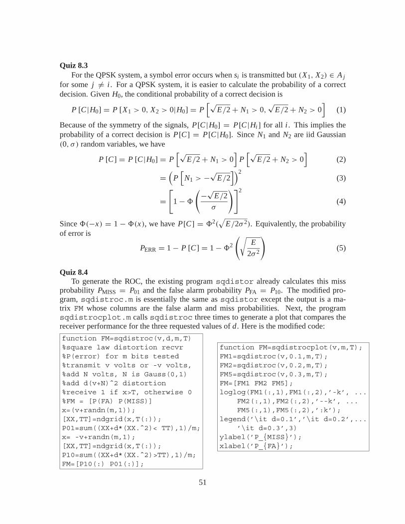
Quiz 8.4To generate the ROC, the existing program sqdistor already calculates this miss
probability PMISS = P01 and the false alarm probability PFA = P10. The modified pro-gram, sqdistroc.m is essentially the same as sqdistor except the output is a ma-trix FM whose columns are the false alarm and miss probabilities. Next, the programsqdistrocplot.m calls sqdistroc three times to generate a plot that compares thereceiver performance for the three requested values of d . Here is the modified code:
function FM=sqdistroc(v,d,m,T)%square law distortion recvr%P(error) for m bits tested%transmit v volts or -v volts,%add N volts, N is Gauss(0,1)%add d(v+N)ˆ2 distortion%receive 1 if x>T, otherwise 0%FM = [P(FA) P(MISS)]x=(v+randn(m,1));[XX,TT]=ndgrid(x,T(:));P01=sum((XX+d*(XX.ˆ2)< TT),1)/m;x= -v+randn(m,1);[XX,TT]=ndgrid(x,T(:));P10=sum((XX+d*(XX.ˆ2)>TT),1)/m;FM=[P10(:) P01(:)];
function FM=sqdistrocplot(v,m,T);FM1=sqdistroc(v,0.1,m,T);FM2=sqdistroc(v,0.2,m,T);FM5=sqdistroc(v,0.3,m,T);FM=[FM1 FM2 FM5];loglog(FM1(:,1),FM1(:,2),’-k’, ...
FM2(:,1),FM2(:,2),’--k’, ...FM5(:,1),FM5(:,2),’:k’);
legend(’\it d=0.1’,’\it d=0.2’,...’\it d=0.3’,3)
ylabel(’P_{MISS}’);xlabel(’P_{FA}’);
51
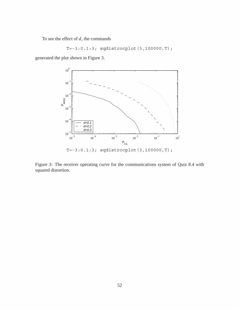
To see the effect of d , the commands
T=-3:0.1:3; sqdistrocplot(3,100000,T);
generated the plot shown in Figure 3.
10−5
10−4
10−3
10−2
10−1
100
10−5
10−4
10−3
10−2
10−1
100
PM
ISS
PFA
d=0.1 d=0.2 d=0.3
T=-3:0.1:3; sqdistrocplot(3,100000,T);
Figure 3: The receiver operating curve for the communications system of Quiz 8.4 withsquared distortion.
52
Quiz Solutions – Chapter 9
Quiz 9.1
(1) First, we calculate the marginal PDF for 0 ≤ y ≤ 1:
fY (y) =∫ y
02(y + x) dx = 2xy + x2
∣∣∣x=y
x=0= 3y2 (1)
This implies the conditional PDF of X given Y is
fX |Y (x |y) = fX,Y (x, y)
fY (y)={
23y + 2x
3y2 0 ≤ x ≤ y
0 otherwise(2)
(2) The minimum mean square error estimate of X given Y = y is
xM(y) = E [X |Y = y] =∫ y
0
(2x
3y+ 2x2
3y2
)dx = 5y/9 (3)
Thus the MMSE estimator of X given Y is X M(Y ) = 5Y/9.
(3) To obtain the conditional PDF fY |X (y|x), we need the marginal PDF fX (x). For0 ≤ x ≤ 1,
fX (x) =∫ 1
x2(y + x) dy = y2 + 2xy
∣∣∣y=1
y=x= 1+ 2x − 3x2 (4)
(5)
For 0 ≤ x ≤ 1, the conditional PDF of Y given X is
fY |X (y|x) ={
2(y+x)
1+2x−3x2 x ≤ y ≤ 10 otherwise
(6)
(4) The MMSE estimate of Y given X = x is
yM(x) = E [Y |X = x] =∫ 1
x
2y2 + 2xy
1+ 2x − 3x2dy (7)
= 2y3/3+ xy2
1+ 2x − 3x2
∣∣∣∣y=1
y=x(8)
= 2+ 3x − 5x3
3+ 6x − 9x2(9)
53

Quiz 9.2
(1) Since the expectation of the sum equals the sum of the expectations,
E [R] = E [T ]+ E [X ] = 0 (1)
(2) Since T and X are independent, the variance of the sum R = T + X is
Var[R] = Var[T ] + Var[X ] = 9+ 3 = 12 (2)
(3) Since T and R have expected values E[R] = E[T ] = 0,
Cov [T, R] = E [T R] = E [T (T + X)] = E[T 2]+ E [T X ] (3)
Since T and X are independent and have zero expected value, E[T X ] = E[T ]E[X ] =0 and E[T 2] = Var[T ]. Thus Cov[T, R] = Var[T ] = 9.
(4) From Definition 4.8, the correlation coefficient of T and R is
ρT,R = Cov [T, R]√Var[R]Var[T ] =
σT
σR= √3/2 (4)
(5) From Theorem 9.4, the optimum linear estimate of T given R is
TL(R) = ρT,RσT
σR(R − E [R])+ E [T ] (5)
Since E[R] = E[T ] = 0 and ρT,R = σT /σR ,
TL(R) = σ 2T
σ 2R
R = σ 2T
σ 2T + σ 2
X
R = 3
4R (6)
Hence a∗ = 3/4 and b∗ = 0.
(6) By Theorem 9.4, the mean square error of the linear estimate is
e∗L = Var[T ](1− ρ2T,R) = 9(1− 3/4) = 9/4 (7)
Quiz 9.3When R = r , the conditional PDF of X = Y−40−40 log10 r is Gaussian with expected
value −40− 40 log10 r and variance 64. The conditional PDF of X given R is
fX |R (x |r) = 1√128π
e−(x+40+40 log10 r)2/128 (1)
54
From the conditional PDF fX |R(x |r), we can use Definition 9.2 to write the ML estimateof R given X = x as
rML(x) = arg maxr≥0
fX |R (x |r) (2)
We observe that fX |R(x |r) is maximized when the exponent (x + 40 + 40 log10 r)2 isminimized. This minimum occurs when the exponent is zero, yielding
log10 r = −1− x/40 (3)
orrML(x) = (0.1)10−x/40 m (4)
If the result doesn’t look correct, note that a typical figure for the signal strength might bex = −120 dB. This corresponds to a distance estimate of rML(−120) = 100 m.
For the MAP estimate, we observe that the joint PDF of X and R is
fX,R (x, r) = fX |R (x |r) fR (r) = 1
106√
32πre−(x+40+40 log10 r)2/128 (5)
From Theorem 9.6, the MAP estimate of R given X = x is the value of r that maximizesfX,R(x, r). That is,
rMAP(x) = arg max0≤r≤1000
fX,R (x, r) (6)
Note that we have included the constraint r ≤ 1000 in the maximization to highlight thefact that under our probability model, R ≤ 1000 m. Setting the derivative of fX,R(x, r)
with respect to r to zero yields
e−(x+40+40 log10 r)2/128[
1− 80 log10 e
128(x + 40+ 40 log10 r)
]= 0 (7)
Solving for r yields
r = 10
(1
25 log10 e−1)10−x/40 = (0.1236)10−x/40 (8)
This is the MAP estimate of R given X = x as long as r ≤ 1000 m. When x ≤ −156.3 dB,the above estimate will exceed 1000 m, which is not possible in our probability model.Hence, the complete description of the MAP estimate is
rMAP(x) ={
1000 x < −156.3(0.1236)10−x/40 x ≥ −156.3
(9)
For example, if x = −120dB, then rMAP(−120) = 123.6 m. When the measured signalstrength is not too low, the MAP estimate is 23.6% larger than the ML estimate. This re-flects the fact that large values of R are a priori more probable than small values. However,for very low signal strengths, the MAP estimate takes into account that the distance cannever exceed 1000 m.
55
Quiz 9.4
(1) From Theorem 9.4, the LMSE estimate of X2 given Y2 is X2(Y2) = a∗Y2+b∗ where
a∗ = Cov [X2, Y2]
Var[Y2] , b∗ = µX2 − a∗µY2 . (1)
Because E[X] = E[Y] = 0,
Cov [X2, Y2] = E [X2Y2] = E [X2(X2 +W2)] = E[
X22
]= 1 (2)
Var[Y2] = Var[X2] + Var[W2] = E[
X22
]+ E
[W 2
2
]= 1.1 (3)
It follows that a∗ = 1/1.1. Because µX2 = µY2 = 0, it follows that b∗ = 0. Finally,to compute the expected square error, we calculate the correlation coefficient
ρX2,Y2 =Cov [X2, Y2]
σX2σY2
= 1√1.1
(4)
The expected square error is
e∗L = Var[X2](1− ρ2X2,Y2
) = 1− 1
1.1= 1
11= 0.0909 (5)
(2) Since Y = X +W and E[X] = E[W] = 0, it follows that E[Y] = 0. Thus we canapply Theorem 9.7. Note that X and W have correlation matrices
RX =[
1 −0.9−0.9 1
], RW =
[0.1 00 0.1
]. (6)
In terms of Theorem 9.7, n = 2 and we wish to estimate X2 given the observationvector Y = [Y1 Y2
]′. To apply Theorem 9.7, we need to find RY and RYX2 .
RY = E[YY′
] = E[(X+W)(X′ +W′)
](7)
= E[XX′ + XW′ +WX′ +WW′
]. (8)
Because X and W are independent, E[XW′] = E[X]E[W′] = 0. Similarly, E[WX′] =0. This implies
RY = E[XX′
]+ E[WW′
] = RX + RW =[
1.1 −0.9−0.9 1.1
]. (9)
In addition, we need to find
RYX2 = E [YX2] =[
E [Y1 X2]E [Y2 X2]
]=[
E [(X1 +W1)X2]E [(X2 +W2)X2]
]. (10)
56
Since X and W are independent vectors, E[W1 X2] = E[W1]E[X2] = 0 and E[W2 X2] =0. Thus
RYX2 =[
E[X1 X2]E[X2
2
] ] = [−0.91
]. (11)
By Theorem 9.7,
a = R−1Y RYX2 =
[−0.2250.725
](12)
Therefore, the optimum linear estimator of X2 given Y1 and Y2 is
X L = a′Y = −0.225Y1 + 0.725Y2. (13)
The mean square error is
Var [X2]− a′RYX2 = Var [X ]− a1rY1,X2 − a2rY2,X2 = 0.0725. (14)
Quiz 9.5Since X and W have zero expected value, Y also has zero expected value. Thus, by
Theorem 9.7, X L(Y) = a′Y where a = R−1Y RYX . Since X and W are independent,
E[WX ] = 0 and E[XW′] = 0′. This implies
RYX = E [YX ] = E [(1X +W)X ] = 1E[
X2]= 1. (1)
By the same reasoning, the correlation matrix of Y is
RY = E[YY′
] = E[(1X +W)(1′X +W′)
](2)
= 11′E[
X2]+ 1E
[XW′
]+ E [WX ] 1′ + E[WW′
](3)
= 11′ + RW (4)
Note that 11′ is a 20× 20 matrix with every entry equal to 1. Thus,
a = R−1Y RYX =
(11′ + RW
)−1 1 (5)
and the optimal linear estimator is
X L(Y) = 1′(11′ + RW
)−1 Y (6)
The mean square error is
e∗L = Var[X ] − a′RYX = 1− 1′(11′ + RW
)−1 1 (7)
Now we note that RW has i, j th entry RW(i, j) = c|i− j |−1. The question we must addressis what value c minimizes e∗L . This problem is atypical in that one does not usually get
57

to choose the correlation structure of the noise. However, we will see that the answer issomewhat instructive.
We note that the answer is not obviously apparent from Equation (7). In particular, weobserve that Var[Wi ] = RW(i, i) = 1/c. Thus, when c is small, the noises Wi have highvariance and we would expect our estimator to be poor. On the other hand, if c is largeWi and W j are highly correlated and the separate measurements of X are very dependent.This would suggest that large values of c will also result in poor MSE. If this argument isnot clear, consider the extreme case in which every Wi and W j have correlation coefficientρi j = 1. In this case, our 20 measurements will be all the same and one measurement is asgood as 20 measurements.
To find the optimal value of c, we write a MATLAB function mquiz9(c) to calculatethe MSE for a given c and second function that finds plots the MSE for a range of valuesof c.
function [mse,af]=mquiz9(c);v1=ones(20,1);RW=toeplitz(c.ˆ((0:19)-1));RY=(v1*(v1’)) +RW;af=(inv(RY))*v1;mse=1-((v1’)*af);
function cmin=mquiz9minc(c);msec=zeros(size(c));for k=1:length(c),
[msec(k),af]=mquiz9(c(k));endplot(c,msec);xlabel(’c’);ylabel(’e_Lˆ*’);[msemin,optk]=min(msec);cmin=c(optk);
Note in mquiz9 that v1 corresponds to the vector 1 of all ones. The following commandsfinds the minimum c and also produces the following graph:
>> c=0.01:0.01:0.99;>> mquiz9minc(c)ans =
0.4500
0 0.5 10.2
0.4
0.6
0.8
1
c
e L*
As we see in the graph, both small values and large values of c result in large MSE.
58
Quiz Solutions – Chapter 10
Quiz 10.1There are many correct answers to this question. A correct answer specifies enough
random variables to specify the sample path exactly. One choice for an alternate set ofrandom variables that would specify m(t, s) is
• m(0, s), the number of ongoing calls at the start of the experiment
• N , the number of new calls that arrive during the experiment
• X1, . . . , X N , the interarrival times of the N new arrivals
• H , the number of calls that hang up during the experiment
• D1, . . . , DH , the call completion times of the H calls that hang up
Quiz 10.2
(1) We obtain a continuous time, continuous valued process when we record the temper-ature as a continuous waveform over time.
(2) If at every moment in time, we round the temperature to the nearest degree, then weobtain a continuous time, discrete valued process.
(3) If we sample the process in part (a) every T seconds, then we obtain a discrete time,continuous valued process.
(4) Rounding the samples in part (c) to the nearest integer degree yields a discrete time,discrete valued process.
Quiz 10.3
(1) Each resistor has resistance R in ohms with uniform PDF
fR (r) ={
0.01 950 ≤ r ≤ 10500 otherwise
(1)
The probability that a test produces a 1% resistor is
p = P [990 ≤ R ≤ 1010] =∫ 1010
990(0.01) dr = 0.2 (2)
59
(2) In t seconds, exactly t resistors are tested. Each resistor is a 1% resistor with proba-bility p, independent of any other resistor. Consequently, the number of 1% resistorsfound has the binomial PMF
PN (t) (n) ={ ( t
n
)pn(1− p)t−n n = 0, 1, . . . , t
0 otherwise(3)
(3) First we will find the PMF of T1. This problem is easy if we view each resistor testas an independent trial. A success occurs on a trial with probability p if we find a1% resistor. The first 1% resistor is found at time T1 = t if we observe failures ontrials 1, . . . , t − 1 followed by a success on trial t . Hence, just as in Example 2.11,T1 has the geometric PMF
PT1 (t) ={
(1− p)t−1 p t = 1, 2, . . .
9 otherwise(4)
Since p = 0.2, the probability the first 1% resistor is found in exactly five seconds isPT1(5) = (0.8)4(0.2) = 0.08192.
(4) From Theorem 2.5, a geometric random variable with success probability p has ex-pected value 1/p. In this problem, E[T1] = 1/p = 5.
(5) Note that once we find the first 1% resistor, the number of additional trials needed tofind the second 1% resistor once again has a geometric PMF with expected value 1/psince each independent trial is a success with probability p. That is, T2 = T1 + T ′where T ′ is independent and identically distributed to T1. Thus
E [T2|T1 = 10] = E [T1|T1 = 10]+ E[T ′|T1 = 10
](5)
= 10+ E[T ′] = 10+ 5 = 15 (6)
Quiz 10.4Since each Xi is a N (0, 1) random variable, each Xi has PDF
fX (i) (x) = 1√2π
e−x2/2 (1)
By Theorem 10.1, the joint PDF of X = [X1 · · · Xn]′
is
fX (x) = fX (1),...,X (n) (x1, . . . , xn) =k∏
i=1
fX (xi ) = 1
(2π)n/2e−(x2
1+···+x2n )/2 (2)
60
Quiz 10.5The first and second hours are nonoverlapping intervals. Since one hour equals 3600
sec and the Poisson process has a rate of 10 packets/sec, the expected number of packetsin each hour is E[Mi ] = α = 36, 000. This implies M1 and M2 are independent Poissonrandom variables each with PMF
PMi (m) ={
αme−α
m! m = 0, 1, 2, . . .
0 otherwise(1)
Since M1 and M2 are independent, the joint PMF of M1 and M2 is
PM1,M2 (m1, m2) = PM1 (m1) PM2 (m2) =
⎧⎪⎪⎨⎪⎪⎩
αm1+m2e−2α
m1!m2! m1 = 0, 1, . . . ;m2 = 0, 1, . . . ,
0 otherwise.
(2)
Quiz 10.6To answer whether N ′(t) is a Poisson process, we look at the interarrival times. Let
X1, X2, . . . denote the interarrival times of the N (t) process. Since we count only even-numbered arrival for N ′(t), the time until the first arrival of the N ′(t) is Y1 = X1 + X2.Since X1 and X2 are independent exponential (λ) random variables, Y1 is an Erlang (n =2, λ) random variable; see Theorem 6.11. Since Yi (t), the i th interarrival time of the N ′(t)process, has the same PDF as Y1(t), we can conclude that the interarrival times of N ′(t)are not exponential random variables. Thus N ′(t) is not a Poisson process.
Quiz 10.7First, we note that for t > s,
X (t)− X (s) = W (t)−W (s)√α
(1)
Since W (t)−W (s) is a Gaussian random variable, Theorem 3.13 states that W (t)−W (s)is Gaussian with expected value
E [X (t)− X (s)] = E [W (t)−W (s)]√α
= 0 (2)
and variance
E[(W (t)−W (s))2
]= E
[(W (t)−W (s))2
]α
= α(t − s)
α(3)
Consider s′ ≤ s < t . Since s ≥ s′, W (t) − W (s) is independent of W (s ′). This implies[W (t) − W (s)]/√α is independent of W (s ′)/
√α for all s ≥ s′. That is, X (t) − X (s) is
independent of X (s ′) for all s ≥ s′. Thus X (t) is a Brownian motion process with varianceVar[X (t)] = t .
61
Quiz 10.8First we find the expected value
µY (t) = µX (t)+ µN (t) = µX (t). (1)
To find the autocorrelation, we observe that since X (t) and N (t) are independent and sinceN (t) has zero expected value, E[X (t)N (t ′)] = E[X (t)]E[N (t ′)] = 0. Since RY (t, τ ) =E[Y (t)Y (t + τ)], we have
RY (t, τ ) = E [(X (t)+ N (t)) (X (t + τ)+ N (t + τ))] (2)
= E [X (t)X (t + τ)]+ E [X (t)N (t + τ)]
+ E [X (t + τ)N (t)]+ E [N (t)N (t + τ)] (3)
= RX (t, τ )+ RN (t, τ ). (4)
Quiz 10.9From Definition 10.14, X1, X2, . . . is a stationary random sequence if for all sets of
time instants n1, . . . , nm and time offset k,
fXn1 ,...,Xnm(x1, . . . , xm) = fXn1+k ,...,Xnm+k (x1, . . . , xm) (1)
Since the random sequence is iid,
fXn1 ,...,Xnm(x1, . . . , xm) = fX (x1) fX (x2) · · · fX (xm) (2)
Similarly, for time instants n1 + k, . . . , nm + k,
fXn1+k ,...,Xnm+k (x1, . . . , xm) = fX (x1) fX (x2) · · · fX (xm) (3)
We can conclude that the iid random sequence is stationary.
Quiz 10.10We must check whether each function R(τ ) meets the conditions of Theorem 10.12:
R(τ ) ≥ 0 R(τ ) = R(−τ) |R(τ )| ≤ R(0) (1)
(1) R1(τ ) = e−|τ | meets all three conditions and thus is valid.
(2) R2(τ ) = e−τ 2also is valid.
(3) R3(τ ) = e−τ cos τ is not valid because
R3(−2π) = e2π cos 2π = e2π > 1 = R3(0) (2)
(4) R4(τ ) = e−τ 2sin τ also cannot be an autocorrelation function because
R4(π/2) = e−π/2 sin π/2 = e−π/2 > 0 = R4(0) (3)
62
Quiz 10.11
(1) The autocorrelation of Y (t) is
RY (t, τ ) = E [Y (t)Y (t + τ)] (1)
= E [X (−t)X (−t − τ)] (2)
= RX (−t − (−t − τ)) = RX (τ ) (3)
Since E[Y (t)] = E[X (−t)] = µX , we can conclude that Y (t) is a wide sensestationary process. In fact, we see that by viewing a process backwards in time, wesee the same second order statistics.
(2) Since X (t) and Y (t) are both wide sense stationary processes, we can check whetherthey are jointly wide sense stationary by seeing if RXY (t, τ ) is just a function of τ .In this case,
RXY (t, τ ) = E [X (t)Y (t + τ)] (4)
= E [X (t)X (−t − τ)] (5)
= RX (t − (−t − τ)) = RX (2t + τ) (6)
Since RXY (t, τ ) depends on both t and τ , we conclude that X (t) and Y (t) are notjointly wide sense stationary. To see why this is, suppose RX (τ ) = e−|τ | so thatsamples of X (t) far apart in time have almost no correlation. In this case, as t getslarger, Y (t) = X (−t) and X (t) become less and less correlated.
Quiz 10.12From the problem statement,
E [X (t)] = E [X (t + 1)] = 0 (1)
E [X (t)X (t + 1)] = 1/2 (2)
Var[X (t)] = Var[X (t + 1)] = 1 (3)
The Gaussian random vector X = [X (t) X (t + 1)]′
has covariance matrix and corre-sponding inverse
CX =[
1 1/21/2 1
]C−1
X =4
3
[1 −1/2−1/2 1
](4)
Since
x′C−1X x = [x0 x1
]′ 43
[1 −1/2−1/2 1
] [x0
x1
]= 4
3
(x2
0 − x0x+x21
)(5)
the joint PDF of X (t) and X (t + 1) is the Gaussian vector PDF
fX (t),X (t+1) (x0, x1) = 1
(2π)n/2[det (CX)]1/2exp
(−1
2x′C−1
X x)
(6)
= 1√3π2
e−23
(x2
0−x0x1+x21
)(7)
63
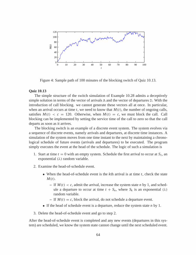
0 10 20 30 40 50 60 70 80 90 1000
20
40
60
80
100
120
t
M(t
)
Figure 4: Sample path of 100 minutes of the blocking switch of Quiz 10.13.
Quiz 10.13The simple structure of the switch simulation of Example 10.28 admits a deceptively
simple solution in terms of the vector of arrivals A and the vector of departures D. With theintroduction of call blocking. we cannot generate these vectors all at once. In particular,when an arrival occurs at time t , we need to know that M(t), the number of ongoing calls,satisfies M(t) < c = 120. Otherwise, when M(t) = c, we must block the call. Callblocking can be implemented by setting the service time of the call to zero so that the calldeparts as soon as it arrives.
The blocking switch is an example of a discrete event system. The system evolves viaa sequence of discrete events, namely arrivals and departures, at discrete time instances. Asimulation of the system moves from one time instant to the next by maintaining a chrono-logical schedule of future events (arrivals and departures) to be executed. The programsimply executes the event at the head of the schedule. The logic of such a simulation is
1. Start at time t = 0 with an empty system. Schedule the first arrival to occur at S1, anexponential (λ) random variable.
2. Examine the head-of-schedule event.
• When the head-of-schedule event is the kth arrival is at time t , check the stateM(t).
– If M(t) < c, admit the arrival, increase the system state n by 1, and sched-ule a departure to occur at time t + Sn , where Sk is an exponential (λ)
random variable.– If M(t) = c, block the arrival, do not schedule a departure event.
• If the head of schedule event is a departure, reduce the system state n by 1.
3. Delete the head-of-schedule event and go to step 2.
After the head-of-schedule event is completed and any new events (departures in this sys-tem) are scheduled, we know the system state cannot change until the next scheduled event.
64
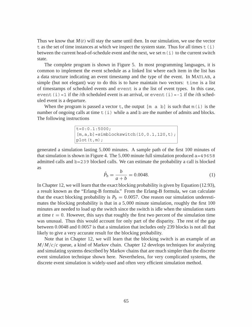
Thus we know that M(t) will stay the same until then. In our simulation, we use the vectort as the set of time instances at which we inspect the system state. Thus for all times t(i)between the current head-of-schedule event and the next, we set m(i) to the current switchstate.
The complete program is shown in Figure 5. In most programming languages, it iscommon to implement the event schedule as a linked list where each item in the list hasa data structure indicating an event timestamp and the type of the event. In MATLAB, asimple (but not elegant) way to do this is to have maintain two vectors: time is a listof timestamps of scheduled events and event is a the list of event types. In this case,event(i)=1 if the i th scheduled event is an arrival, or event(i)=-1 if the i th sched-uled event is a departure.
When the program is passed a vector t, the output [m a b] is such that m(i) is thenumber of ongoing calls at time t(i) while a and b are the number of admits and blocks.The following instructions
t=0:0.1:5000;[m,a,b]=simblockswitch(10,0.1,120,t);plot(t,m);
generated a simulation lasting 5,000 minutes. A sample path of the first 100 minutes ofthat simulation is shown in Figure 4. The 5,000 minute full simulation produced a=49658admitted calls and b=239 blocked calls. We can estimate the probability a call is blockedas
Pb = b
a + b= 0.0048. (1)
In Chapter 12, we will learn that the exact blocking probability is given by Equation (12.93),a result known as the “Erlang-B formula.” From the Erlang-B formula, we can calculatethat the exact blocking probability is Pb = 0.0057. One reason our simulation underesti-mates the blocking probability is that in a 5,000 minute simulation, roughly the first 100minutes are needed to load up the switch since the switch is idle when the simulation startsat time t = 0. However, this says that roughly the first two percent of the simulation timewas unusual. Thus this would account for only part of the disparity. The rest of the gapbetween 0.0048 and 0.0057 is that a simulation that includes only 239 blocks is not all thatlikely to give a very accurate result for the blocking probability.
Note that in Chapter 12, we will learn that the blocking switch is an example of anM/M/c/c queue, a kind of Markov chain. Chapter 12 develops techniques for analyzingand simulating systems described by Markov chains that are much simpler than the discreteevent simulation technique shown here. Nevertheless, for very complicated systems, thediscrete event simulation is widely-used and often very efficient simulation method.
65

function [M,admits,blocks]=simblockswitch(lam,mu,c,t);blocks=0; %total # blocksadmits=0; %total # admitsM=zeros(size(t));n=0; % # in systemtime=[ exponentialrv(lam,1) ];event=[ 1 ]; %first event is an arrivaltimenow=0;tmax=max(t);while (timenow<tmax)
M((timenow<=t)&(t<time(1)))=n;timenow=time(1);eventnow=event(1);event(1)=[ ]; time(1)= [ ]; % clear current eventif (eventnow==1) % arrival
arrival=timenow+exponentialrv(lam,1); % next arrivalb4arrival=time<arrival;event=[event(b4arrival) 1 event(˜b4arrival)];time=[time(b4arrival) arrival time(˜b4arrival)];if n<c %call admittedadmits=admits+1;n=n+1;depart=timenow+exponentialrv(mu,1);b4depart=time<depart;event=[event(b4depart) -1 event(˜b4depart)];time=[time(b4depart) depart time(˜b4depart)];
elseblocks=blocks+1; %one more block, immed departuredisp(sprintf(’Time %10.3d Admits %10d Blocks %10d’,...
timenow,admits,blocks));end
elseif (eventnow==-1) %departuren=n-1;
endend
Figure 5: Discrete event simulation of the blocking switch of Quiz 10.13.
66
Quiz Solutions – Chapter 11
Quiz 11.1By Theorem 11.2,
µY = µX
∫ ∞−∞
h(t)dt = 2∫ ∞
0e−t dt = 2 (1)
Since RX (τ ) = δ(τ ), the autocorrelation function of the output is
RY (τ ) =∫ ∞−∞
h(u)
∫ ∞−∞
h(v)δ(τ + u − v) dv du =∫ ∞−∞
h(u)h(τ + u) du (2)
For τ > 0, we have
RY (τ ) =∫ ∞
0e−ue−τ−u du = e−τ
∫ ∞0
e−2u du = 1
2e−τ (3)
For τ < 0, we can deduce that RY (τ ) = 12e−|τ | by symmetry. Just to be safe though, we
can double check. For τ < 0,
RY (τ ) =∫ ∞−τ
h(u)h(τ + u) du =∫ ∞−τ
e−ue−τ−u du = 1
2eτ (4)
Hence,
RY (τ ) = 1
2e−|τ | (5)
Quiz 11.2The expected value of the output is
µY = µX
∞∑n=−∞
hn = 0.5(1+−1) = 0 (1)
The autocorrelation of the output is
RY [n] =1∑
i=0
1∑j=0
hi h j RX [n + i − j] (2)
= 2RX [n] − RX [n − 1] − RX [n + 1] ={
1 n = 00 otherwise
(3)
Since µY = 0, The variance of Yn is Var[Yn] = E[Y 2n ] = RY [0] = 1.
67
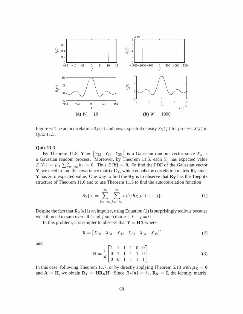
−15 −10 −5 0 5 10 150
0.2
0.4
0.6
f
SX(f
)
−1500−1000 −500 0 500 1000 15000
2
4
6
8x 10
f
SX(f
)
−0.2 −0.1 0 0.1 0.2−5
0
5
10
τ
RX(τ
)
−2 −1 0 1 2
x 10−3
−5
0
5
10
τ
RX(τ
)
(a) W = 10 (b) W = 1000
Figure 6: The autocorrelation RX (τ ) and power spectral density SX ( f ) for process X (t) inQuiz 11.5.
Quiz 11.3By Theorem 11.8, Y = [
Y33 Y34 Y35]′
is a Gaussian random vector since Xn isa Gaussian random process. Moreover, by Theorem 11.5, each Yn has expected valueE[Yn] = µX
∑∞n=−∞ hn = 0. Thus E[Y] = 0. Fo find the PDF of the Gaussian vector
Y, we need to find the covariance matrix CY, which equals the correlation matrix RY sinceY has zero expected value. One way to find the RY is to observe that RY has the Toeplitzstructure of Theorem 11.6 and to use Theorem 11.5 to find the autocorrelation function
RY [n] =∞∑
i=−∞
∞∑j=−∞
hi h j RX [n + i − j]. (1)
Despite the fact that RX [k] is an impulse, using Equation (1) is surprisingly tedious becausewe still need to sum over all i and j such that n + i − j = 0.
In this problem, it is simpler to observe that Y = HX where
X = [X30 X31 X32 X33 X34 X35]′
(2)
and
H = 1
4
⎡⎣1 1 1 1 0 0
0 1 1 1 1 00 0 1 1 1 1
⎤⎦ . (3)
In this case, following Theorem 11.7, or by directly applying Theorem 5.13 with µX = 0and A = H, we obtain RY = HRXH′. Since RX [n] = δn , RX = I, the identity matrix.
68
Thus
CY = RY = HH′ = 1
16
⎡⎣4 3 2
3 4 32 3 4
⎤⎦ . (4)
It follows (very quickly if you use MATLAB for 3× 3 matrix inversion) that
C−1Y = 16
⎡⎣7/12 −1/2 1/12−1/2 1 −1/21/12 −1/2 7/12
⎤⎦ . (5)
Thus, the PDF of Y is
fY (y) = 1
(2π)3/2[det (CY)]1/2exp
(−1
2y′C−1
Y y)
. (6)
A disagreeable amount of algebra will show det(CY) = 3/1024 and that the PDF can be“simplified” to
fY (y) = 16√6π3
exp
[−8
(7
12y2
33 + y234 +
7
12y2
35 − y33y34 + 1
6y33y35 − y34y35
)]. (7)
Equation (7) shows that one of the nicest features of the multivariate Gaussian distributionis that y′C−1
Y y is a very concise representation of the cross-terms in the exponent of fY(y).
Quiz 11.4This quiz is solved using Theorem 11.9 for the case of k = 1 and M = 2. In this case,
Xn =[Xn−1 Xn
]′and
RXn =[
RX [0] RX [1]RX [1] RX [0]
]=[
1.1 0.90.9 1.1
](1)
and
RXn Xn+1 = E
[[Xn−1
Xn
]Xn+1
]=[
RX [2]RX [1]
]=[
0.810.9
]. (2)
The MMSE linear first order filter for predicting Xn+1 at time n is the filter h such that
←−h = R−1
XnRXn Xn+1 =
[1.1 0.90.9 1.1
]−1 [0.810.9
]= 1
400
[81
261
]. (3)
It follows that the filter is h = [261/400 81/400]′
and the MMSE linear predictor is
Xn+1 = 81
400Xn−1 + 261
400Xn. (4)
to find the mean square error, one approach is to follow the method of Example 11.13 andto directly calculate
e∗L = E[(Xn+1 − Xn+1)
2]. (5)
69
This method is workable for this simple problem but becomes increasingly tedious forhigher order filters. Instead, we can derive the mean square error for an arbitary predictionfilter h. Since Xn+1 =←−h ′Xn ,
e∗L = E
[(Xn+1 −←−h ′Xn
)2]
(6)
= E[(Xn+1 −←−h ′Xn)(Xn+1 −←−h ′Xn)
′] (7)
= E[(Xn+1 −←−h ′Xn)(Xn+1 − X′n
←−h )]
(8)
After a bit of algebra, we obtain
e∗L = RX [0] − 2←−h ′RXn Xn+1 +
←−h ′RXn
←−h (9)
(10)
with the substitution←−h = R−1
XnRXn Xn+1 , we obtain
e∗L = RX [0] − R′Xn Xn+1R−1
XnRXn Xn+1 (11)
= RX [0] −←−h ′RXn Xn+1 (12)
Note that this is essentially the same result as Theorem 9.7 with Y = Xn , X = Xn+1 anda′ = ←−h ′. It is noteworthy that the result is derived in a much simpler way in the proof ofTheorem 9.7 by using the orthoginality property of the LMSE estimator.
In any case, the mean square error is
e∗L = RX [0] −←−h ′RXn Xn+1 = 1.1− 1
400
[81 261
] [0.810.9
]= 506
1451= 0.3487. (13)
recalling that the blind estimate would yield a mean square error of Var[X ] = 1.1, we seethat observing Xn−1 and Xn improves the accuracy of our prediction of Xn+1.
Quiz 11.5
(1) By Theorem 11.13(b), the average power of X (t) is
E[
X2(t)]=∫ ∞−∞
SX ( f ) d f =∫ W
−W
5
Wd f = 10 Watts (1)
(2) The autocorrelation function is the inverse Fourier transform of SX ( f ). ConsultingTable 11.1, we note that
SX ( f ) = 101
2Wrect
(f
2W
)(2)
It follows that the inverse transform of SX ( f ) is
RX (τ ) = 10 sinc(2Wτ) = 10sin(2πWτ)
2πWτ(3)
(3) For W = 10 Hz and W = 1 kHZ, graphs of SX ( f ) and RX (τ ) appear in Figure 6.
70
Quiz 11.6In a sampled system, the discrete time impulse δ[n] has a flat discrete Fourier transform.
That is, if RX [n] = 10δ[n], then
SX (φ) =∞∑
n=−∞10δ[n]e− j2πφn = 10 (1)
Thus, RX [n] = 10δ[n]. (This quiz is really lame!)
Quiz 11.7Since Y (t) = X (t − t0),
RXY (t, τ ) = E [X (t)Y (t + τ)] = E [X (t)X (t + τ − t0)] = RX (τ − t0) (1)
We see that RXY (t, τ ) = RXY (τ ) = RX (τ − t0). From Table 11.1, we recall the prop-erty that g(τ − τ0) has Fourier transform G( f )e− j2π f τ0 . Thus the Fourier transform ofRXY (τ ) = RX (τ − t0) = g(τ − t0) is
SXY ( f ) = SX ( f )e− j2π f t0 . (2)
Quiz 11.8We solve this quiz using Theorem 11.17. First we need some preliminary facts. Let
a0 = 5,000 so that
RX (τ ) = 1
a0a0e−a0|τ |. (1)
Consulting with the Fourier transforms in Table 11.1, we see that
SX ( f ) = 1
a0
2a20
a20 + (2π f )2
= 2a0
a20 + (2π f )2
(2)
The RC filter has impulse response h(t) = a1e−a1t u(t), where u(t) is the unit step functionand a1 = 1/RC where RC = 10−4 is the filter time constant. From Table 11.1,
H( f ) = a1
a1 + j2π f(3)
(1) Theorem 11.17,
SXY ( f ) = H( f )SX ( f ) = 2a0a1
[a1 + j2π f ][a2
0 + (2π f )2] . (4)
(2) Again by Theorem 11.17,
SY ( f ) = H∗( f )SXY ( f ) = |H( f )|2 SX ( f ). (5)
71
Note that
|H( f )|2 = H( f )H∗( f ) = a1
(a1 + j2π f )
a1
(a1 − j2π f )= a2
1
a21 + (2π f )2
(6)
Thus,
SY ( f ) = |H( f )|2 SX ( f ) = 2a0a21[
a21 + (2π f )2
] [a2
0 + (2π f )2] (7)
(3) To find the average power at the filter output, we can either use basic calculus andcalculate
∫∞−∞ SY ( f ) d f directly or we can find RY (τ ) as an inverse transform of
SY ( f ). Using partial fractions and the Fourier transform table, the latter method isactually less algebra. In particular, some algebra will show that
SY ( f ) = K0
a20 + (2π f )2
+ K1
a1 + (2π f )2(8)
where
K0 = 2a0a21
a21 − a2
0
, K1 = −2a0a21
a21 − a2
0
. (9)
Thus,
SY ( f ) = K0
2a20
2a20
a20 + (2π f )2
+ K1
2a21
2a21
a1 + (2π f )2. (10)
Consulting with Table 11.1, we see that
RY (τ ) = K0
2a20
a0e−a0|τ | + K1
2a21
a1e−a1|τ | (11)
Substituting the values of K0 and K1, we obtain
RY (τ ) = a21e−a0|τ | − a0a1e−a1|τ |
a21 − a2
0
. (12)
The average power of the Y (t) process is
RY (0) = a1
a1 + a0= 2
3. (13)
Note that the input signal has average power RX (0) = 1. Since the RC filter has a 3dBbandwidth of 10,000 rad/sec and the signal X (t) has most of its its signal energy below5,000 rad/sec, the output signal has almost as much power as the input.
72
Quiz 11.9This quiz implements an example of Equations (11.146) and (11.147) for a system in
which we filter Y (t) = X (t) + N (t) to produce an optimal linear estimate of X (t). Thesolution to this quiz is just to find the filter H( f ) using Equation (11.146) and to calculatethe mean square error eL∗ using Equation (11.147).
Comment: Since the text omitted the derivations of Equations (11.146) and (11.147), wenote that Example 10.24 showed that
RY (τ ) = RX (τ )+ RN (τ ), RY X (τ ) = RX (τ ). (1)
Taking Fourier transforms, it follows that
SY ( f ) = SX ( f )+ SN ( f ), SY X ( f ) = SX ( f ). (2)
Now we can go on to the quiz, at peace with the derivations.
(1) Since µN = 0, RN (0) = Var[N ] = 1. This implies
RN (0) =∫ ∞−∞
SN ( f ) d f =∫ B
−BN0 d f = 2N0 B (3)
Thus N0 = 1/(2B). Because the noise process N (t) has constant power RN (0) = 1,decreasing the single-sided bandwidth B increases the power spectral density of thenoise over frequencies | f | < B.
(2) Since RX (τ ) = sinc(2Wτ), where W = 5,000 Hz, we see from Table 11.1 that
SX ( f ) = 1
104rect
(f
104
). (4)
The noise power spectral density can be written as
SN ( f ) = N0 rect
(f
2B
)= 1
2Brect
(f
2B
), (5)
From Equation (11.146), the optimal filter is
H( f ) = SX ( f )
SX ( f )+ SN ( f )=
1104 rect
(f
104
)1
104 rect(
f104
)+ 1
2B rect(
f2B
) . (6)
73
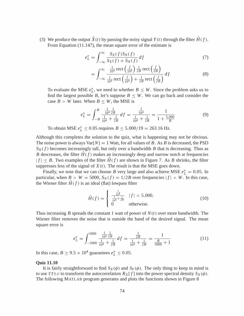
(3) We produce the output X(t) by passing the noisy signal Y (t) through the filter H( f ).From Equation (11.147), the mean square error of the estimate is
e∗L =∫ ∞−∞
SX ( f )SN ( f )
SX ( f )+ SN ( f )d f (7)
=∫ ∞−∞
1104 rect
(f
104
)1
2B rect(
f2B
)1
104 rect(
f104
)+ 1
2B rect(
f2B
) d f. (8)
To evaluate the MSE e∗L , we need to whether B ≤ W . Since the problem asks us tofind the largest possible B, let’s suppose B ≤ W . We can go back and consider thecase B > W later. When B ≤ W , the MSE is
e∗L =∫ B
−B
1104
12B
1104 + 1
2B
d f =1
104
1104 + 1
2B
= 1
1+ 5,000B
(9)
To obtain MSE e∗L ≤ 0.05 requires B ≤ 5,000/19 = 263.16 Hz.
Although this completes the solution to the quiz, what is happening may not be obvious.The noise power is always Var[N ] = 1 Watt, for all values of B. As B is decreased, the PSDSN ( f ) becomes increasingly tall, but only over a bandwidth B that is decreasing. Thus asB descreases, the filter H( f ) makes an increasingly deep and narrow notch at frequencies| f | ≤ B. Two examples of the filter H( f ) are shown in Figure 7. As B shrinks, the filtersuppresses less of the signal of X (t). The result is that the MSE goes down.
Finally, we note that we can choose B very large and also achieve MSE e∗L = 0.05. Inparticular, when B > W = 5000, SN ( f ) = 1/2B over frequencies | f | < W . In this case,the Wiener filter H( f ) is an ideal (flat) lowpass filter
H( f ) =⎧⎨⎩
1104
1104+ 1
2B| f | < 5,000,
0 otherwise.(10)
Thus increasing B spreads the constant 1 watt of power of N (t) over more bandwidth. TheWiener filter removes the noise that is outside the band of the desired signal. The meansquare error is
e∗L =∫ 5000
−5000
1104
12B
1104 + 1
2B
d f =1
2B1
104 + 12B
= 1B
5000 + 1(11)
In this case, B ≥ 9.5× 10⁴ guarantees e∗L ≤ 0.05.
Quiz 11.10It is fairly straightforward to find SX (φ) and SY (φ). The only thing to keep in mind is
to use fftc to transform the autocorrelation RX [ f ] into the power spectral density SX (φ).The following MATLAB program generates and plots the functions shown in Figure 8
74

−5000 −2000 0 2000 50000
0.5
1
f
H(f
)−5000 −2000 0 2000 5000
0
0.5
1
f
H(f
)
B = 500 B = 2500
Figure 7: Wiener filter for Quiz 11.9.
%mquiz11.mN=32;rx=[2 4 2]; SX=fftc(rx,N); %autocorrelation and PSDstem(0:N-1,abs(sx));xlabel(’n’);ylabel(’S_X(n/N)’);h2=0.5*[1 1]; H2=fft(h2,N); %impulse/filter response: M=2SY2=SX.* ((abs(H2)).ˆ2);figure; stem(0:N-1,abs(SY2)); %PSD of Y for M=2xlabel(’n’);ylabel(’S_{Y_2}(n/N)’);h10=0.1*ones(1,10); H10=fft(h10,N); %impulse/filter response: M=10SY10=sx.*((abs(H10)).ˆ2);figure; stem(0:N-1,abs(SY10));xlabel(’n’);ylabel(’S_{Y_{10}}(n/N)’);
Relative to M = 2, when M = 10, the filter H(φ) filters out almost all of the highfrequency components of X (t). In the context of Example 11.26, the low pass movingaverage filter for M = 10 removes the high frquency components and results in a filteroutput that varies very slowly.
As an aside, note that the vectors SX, SY2 and SY10 in mquiz11 should all be real-valued vectors. However, the finite numerical precision of MATLAB results in tiny imagi-nary parts. Although these imaginary parts have no computational significance, they tendto confuse the stem function. Hence, we generate stem plots of the magnitude of eachpower spectral density.
75
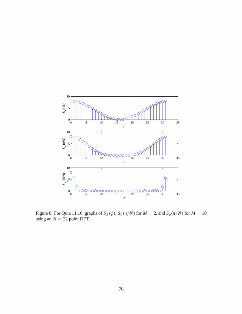
0 5 10 15 20 25 30 350
5
10
n
SX(n
/N)
0 5 10 15 20 25 30 350
5
10
n
SY
2(n/N
)
0 5 10 15 20 25 30 350
5
10
n
SY
10
(n/N
)
Figure 8: For Quiz 11.10, graphs of SX (φ), SY (n/N ) for M = 2, and Sφ(n/N ) for M = 10using an N = 32 point DFT.
76

Quiz Solutions – Chapter 12
Quiz 12.1The system has two states depending on whether the previous packet was received in
error. From the problem statement, we are given the conditional probabilities
P[Xn+1 = 0|Xn = 0
] = 0.99 P[Xn+1 = 1|Xn = 1
] = 0.9 (1)
Since each Xn must be either 0 or 1, we can conclude that
P[Xn+1 = 1|Xn = 0
] = 0.01 P[Xn+1 = 0|Xn = 1
] = 0.1 (2)
These conditional probabilities correspond to the transition matrix and Markov chain:
0 1
0.01
0.1
0.99 0.9
P =[
0.99 0.010.10 0.90
](3)
Quiz 12.2From the problem statement, the Markov chain and the transition matrix are
0 1 1
0.6 0.2
0.2 0.6
0.4 0.6 0.4
P =⎡⎣0.4 0.6 0
0.2 0.6 0.20 0.6 0.4
⎤⎦ (1)
The eigenvalues of P are
λ1 = 0 λ2 = 0.4 λ3 = 1 (2)
We can diagonalize P into
P = S−1DS =⎡⎣−0.6 0.5 1
0.4 0 1−0.6 −0.5 1
⎤⎦⎡⎣λ1 0 0
0 λ2 00 0 λ3
⎤⎦⎡⎣−0.5 1 −0.5
1 0 −10.2 0.6 0.2
⎤⎦ (3)
where si , the i th row of S, is the left eigenvector of P satisfying siP = λisi . Algebra willverify that the n-step transition matrix is
Pn = S−1DnS =⎡⎣0.2 0.6 0.2
0.2 0.6 0.20.2 0.6 0.2
⎤⎦+ (0.4)n
⎡⎣ 0.5 0 −0.5
0 0 0−0.5 0 0.5
⎤⎦ (4)
Quiz 12.3The Markov chain describing the factory status and the corresponding state transition
matrix are
77
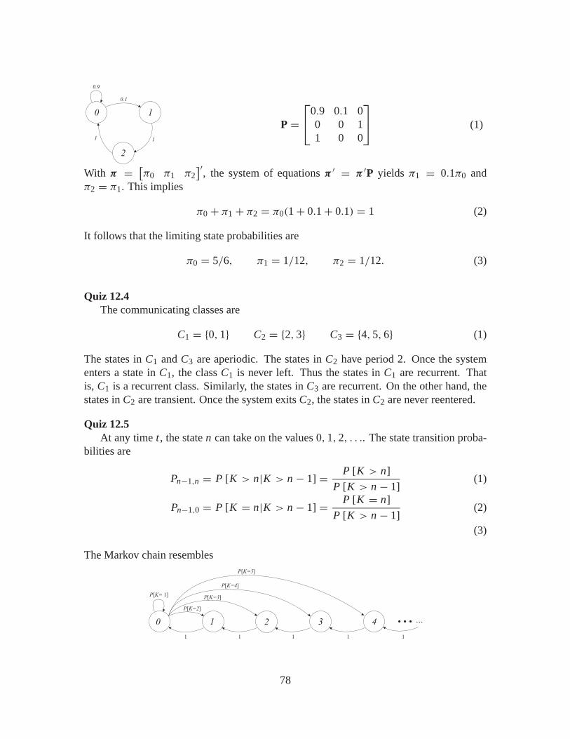
2
0 1
0.9
0.1
11
P =⎡⎣0.9 0.1 0
0 0 11 0 0
⎤⎦ (1)
With π = [π0 π1 π2
]′, the system of equations π ′ = π ′P yields π1 = 0.1π0 and
π2 = π1. This implies
π0 + π1 + π2 = π0(1+ 0.1+ 0.1) = 1 (2)
It follows that the limiting state probabilities are
π0 = 5/6, π1 = 1/12, π2 = 1/12. (3)
Quiz 12.4The communicating classes are
C1 = {0, 1} C2 = {2, 3} C3 = {4, 5, 6} (1)
The states in C1 and C3 are aperiodic. The states in C2 have period 2. Once the systementers a state in C1, the class C1 is never left. Thus the states in C1 are recurrent. Thatis, C1 is a recurrent class. Similarly, the states in C3 are recurrent. On the other hand, thestates in C2 are transient. Once the system exits C2, the states in C2 are never reentered.
Quiz 12.5At any time t , the state n can take on the values 0, 1, 2, . . .. The state transition proba-
bilities are
Pn−1,n = P [K > n|K > n − 1] = P [K > n]
P [K > n − 1](1)
Pn−1,0 = P [K = n|K > n − 1] = P [K = n]
P [K > n − 1](2)
(3)
The Markov chain resembles
0 1
P K=2[ ]
P K=[ 1]
3 4
P K=4[ ]
2
P K=3[ ]
P K=5[ ]
1 1 1 1 1
…...
78
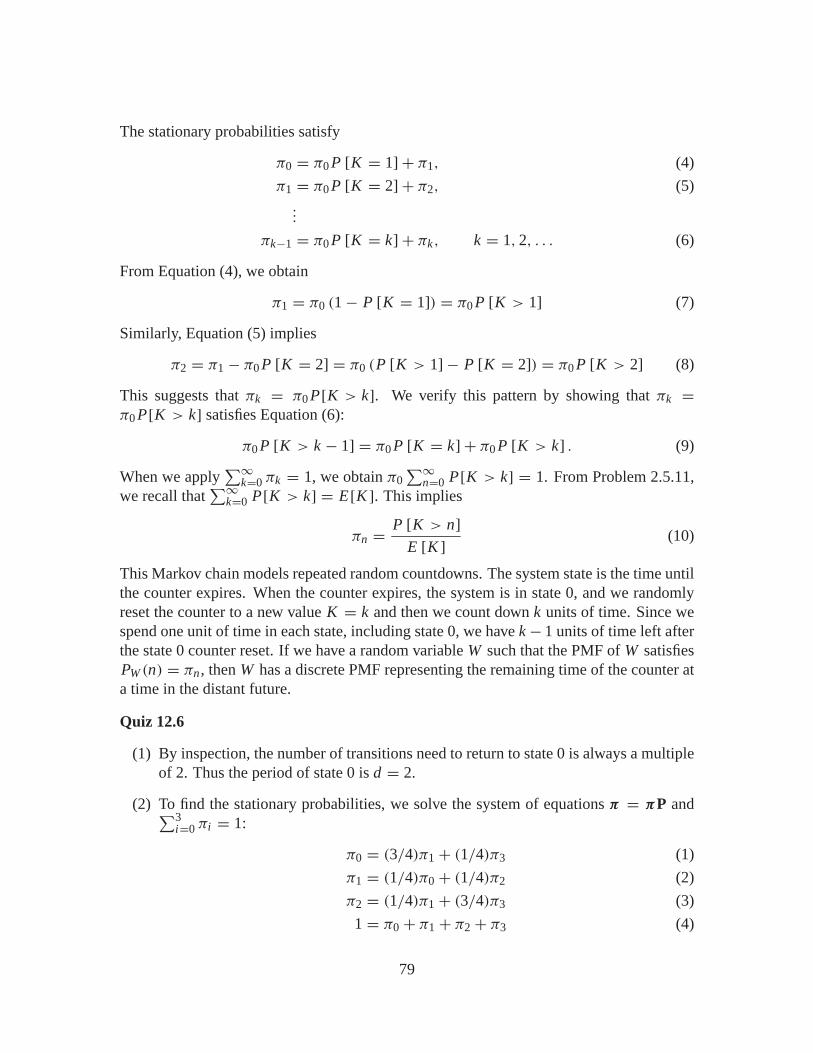
The stationary probabilities satisfy
π0 = π0 P [K = 1]+ π1, (4)
π1 = π0 P [K = 2]+ π2, (5)...
πk−1 = π0 P [K = k]+ πk, k = 1, 2, . . . (6)
From Equation (4), we obtain
π1 = π0 (1− P [K = 1]) = π0 P [K > 1] (7)
Similarly, Equation (5) implies
π2 = π1 − π0 P [K = 2] = π0 (P [K > 1]− P [K = 2]) = π0 P [K > 2] (8)
This suggests that πk = π0 P[K > k]. We verify this pattern by showing that πk =π0 P[K > k] satisfies Equation (6):
π0 P [K > k − 1] = π0 P [K = k]+ π0 P [K > k] . (9)
When we apply∑∞
k=0 πk = 1, we obtain π0∑∞
n=0 P[K > k] = 1. From Problem 2.5.11,we recall that
∑∞k=0 P[K > k] = E[K ]. This implies
πn = P [K > n]
E [K ](10)
This Markov chain models repeated random countdowns. The system state is the time untilthe counter expires. When the counter expires, the system is in state 0, and we randomlyreset the counter to a new value K = k and then we count down k units of time. Since wespend one unit of time in each state, including state 0, we have k− 1 units of time left afterthe state 0 counter reset. If we have a random variable W such that the PMF of W satisfiesPW (n) = πn , then W has a discrete PMF representing the remaining time of the counter ata time in the distant future.
Quiz 12.6
(1) By inspection, the number of transitions need to return to state 0 is always a multipleof 2. Thus the period of state 0 is d = 2.
(2) To find the stationary probabilities, we solve the system of equations π = πP and∑3i=0 πi = 1:
π0 = (3/4)π1 + (1/4)π3 (1)
π1 = (1/4)π0 + (1/4)π2 (2)
π2 = (1/4)π1 + (3/4)π3 (3)
1 = π0 + π1 + π2 + π3 (4)
79
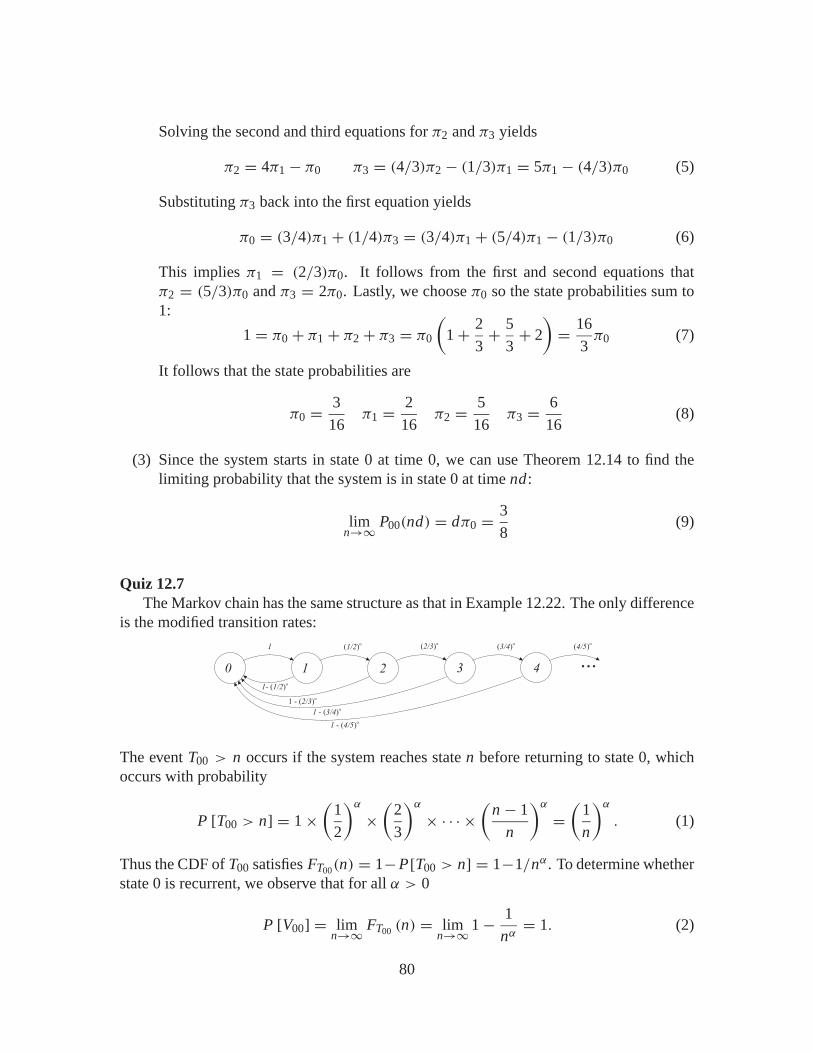
Solving the second and third equations for π2 and π3 yields
π2 = 4π1 − π0 π3 = (4/3)π2 − (1/3)π1 = 5π1 − (4/3)π0 (5)
Substituting π3 back into the first equation yields
π0 = (3/4)π1 + (1/4)π3 = (3/4)π1 + (5/4)π1 − (1/3)π0 (6)
This implies π1 = (2/3)π0. It follows from the first and second equations thatπ2 = (5/3)π0 and π3 = 2π0. Lastly, we choose π0 so the state probabilities sum to1:
1 = π0 + π1 + π2 + π3 = π0
(1+ 2
3+ 5
3+ 2
)= 16
3π0 (7)
It follows that the state probabilities are
π0 = 3
16π1 = 2
16π2 = 5
16π3 = 6
16(8)
(3) Since the system starts in state 0 at time 0, we can use Theorem 12.14 to find thelimiting probability that the system is in state 0 at time nd:
limn→∞ P00(nd) = dπ0 = 3
8(9)
Quiz 12.7The Markov chain has the same structure as that in Example 12.22. The only difference
is the modified transition rates:
0 1
1
3 4
( )2/3�
1 - ( )2/3�
( )3/4�
1 - 3/4( )�
( )4/5�
1 - 4/5( )�
2
( )1/2�
1- 1/2( )�
…
The event T00 > n occurs if the system reaches state n before returning to state 0, whichoccurs with probability
P [T00 > n] = 1×(
1
2
)α
×(
2
3
)α
× · · · ×(
n − 1
n
)α
=(
1
n
)α
. (1)
Thus the CDF of T00 satisfies FT00(n) = 1−P[T00 > n] = 1−1/nα. To determine whetherstate 0 is recurrent, we observe that for all α > 0
P [V00] = limn→∞ FT00 (n) = lim
n→∞ 1− 1
nα= 1. (2)
80
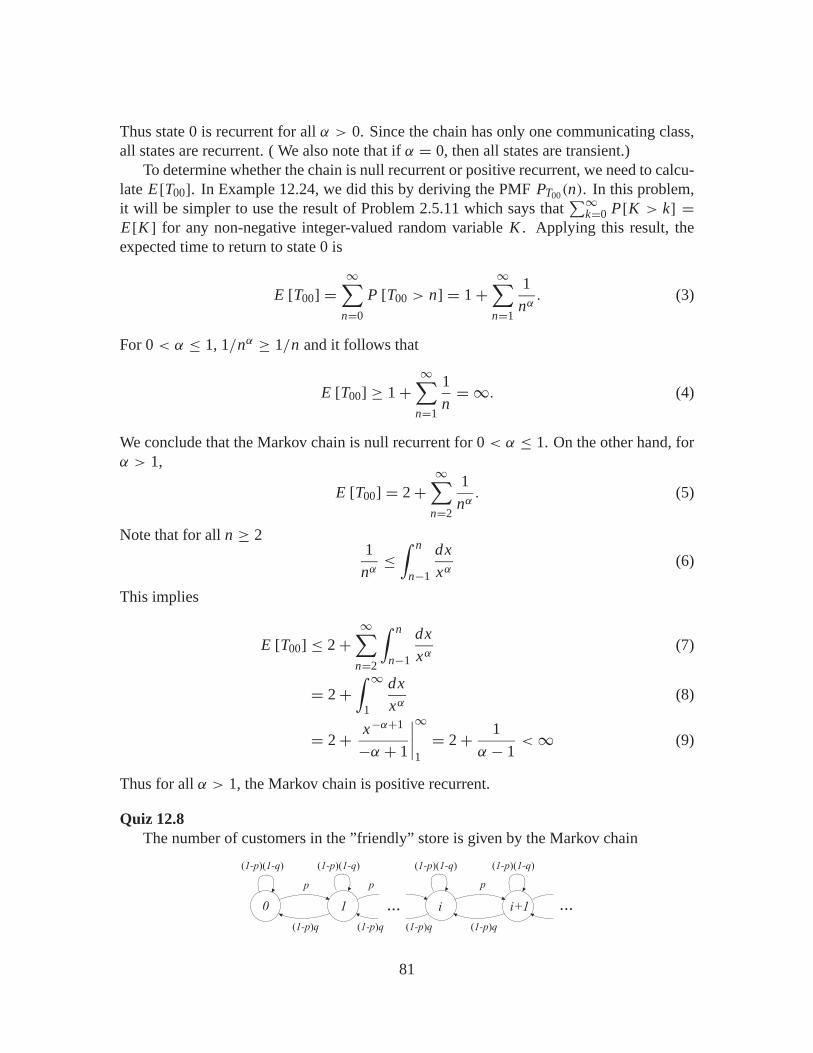
Thus state 0 is recurrent for all α > 0. Since the chain has only one communicating class,all states are recurrent. ( We also note that if α = 0, then all states are transient.)
To determine whether the chain is null recurrent or positive recurrent, we need to calcu-late E[T00]. In Example 12.24, we did this by deriving the PMF PT00(n). In this problem,it will be simpler to use the result of Problem 2.5.11 which says that
∑∞k=0 P[K > k] =
E[K ] for any non-negative integer-valued random variable K . Applying this result, theexpected time to return to state 0 is
E [T00] =∞∑
n=0
P [T00 > n] = 1+∞∑
n=1
1
nα. (3)
For 0 < α ≤ 1, 1/nα ≥ 1/n and it follows that
E [T00] ≥ 1+∞∑
n=1
1
n= ∞. (4)
We conclude that the Markov chain is null recurrent for 0 < α ≤ 1. On the other hand, forα > 1,
E [T00] = 2+∞∑
n=2
1
nα. (5)
Note that for all n ≥ 21
nα≤∫ n
n−1
dx
xα(6)
This implies
E [T00] ≤ 2+∞∑
n=2
∫ n
n−1
dx
xα(7)
= 2+∫ ∞
1
dx
xα(8)
= 2+ x−α+1
−α + 1
∣∣∣∣∞
1= 2+ 1
α − 1<∞ (9)
Thus for all α > 1, the Markov chain is positive recurrent.
Quiz 12.8The number of customers in the ”friendly” store is given by the Markov chain
1 i i+1
p p p
( )( )1-p 1-q ( )( )1-p 1-q ( )( )1-p 1-q ( )( )1-p 1-q
( )1-p q ( )1-p q ( )1-p q ( )1-p q
0 ��� ���
81
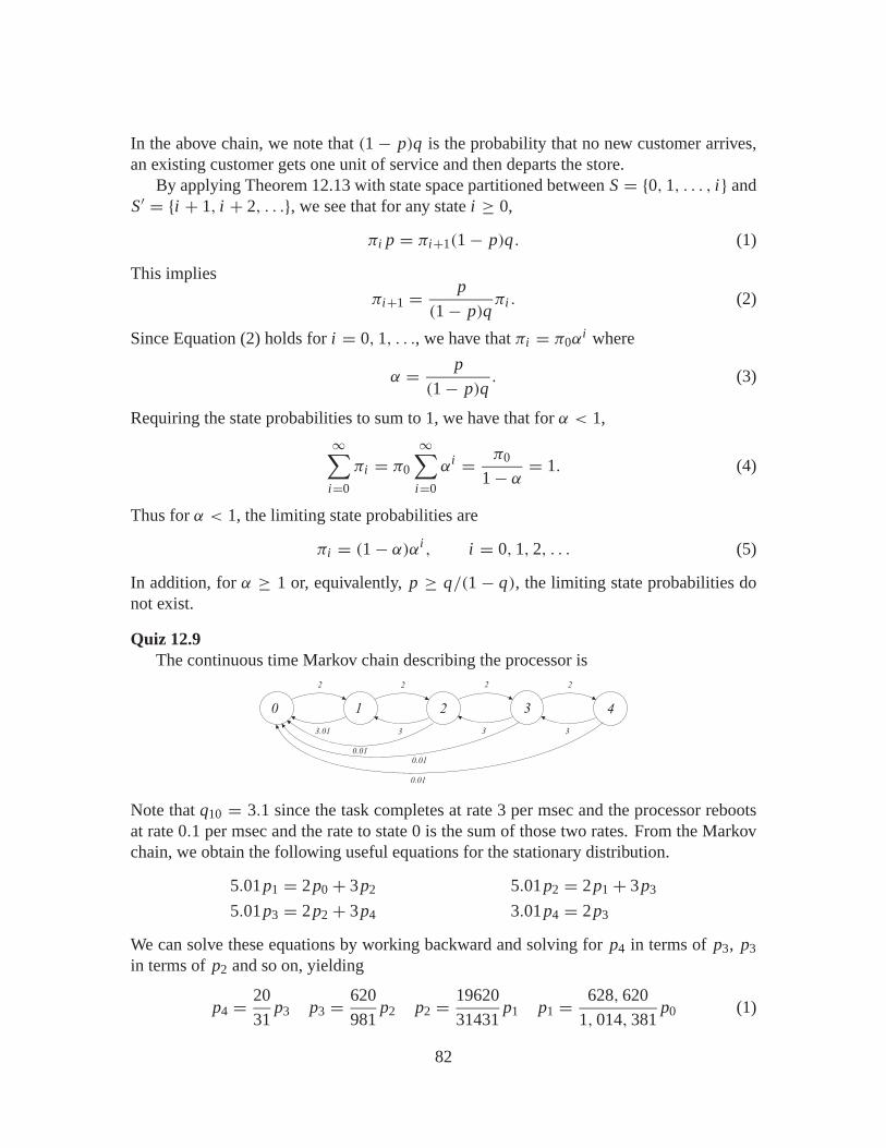
In the above chain, we note that (1 − p)q is the probability that no new customer arrives,an existing customer gets one unit of service and then departs the store.
By applying Theorem 12.13 with state space partitioned between S = {0, 1, . . . , i} andS′ = {i + 1, i + 2, . . .}, we see that for any state i ≥ 0,
πi p = πi+1(1− p)q. (1)
This implies
πi+1 = p
(1− p)qπi . (2)
Since Equation (2) holds for i = 0, 1, . . ., we have that πi = π0αi where
α = p
(1− p)q. (3)
Requiring the state probabilities to sum to 1, we have that for α < 1,
∞∑i=0
πi = π0
∞∑i=0
αi = π0
1− α= 1. (4)
Thus for α < 1, the limiting state probabilities are
πi = (1− α)αi , i = 0, 1, 2, . . . (5)
In addition, for α ≥ 1 or, equivalently, p ≥ q/(1 − q), the limiting state probabilities donot exist.
Quiz 12.9The continuous time Markov chain describing the processor is
0 1
2
3.01
3 4
2
3
2
3
2
2
3
0.010.01
0.01
Note that q10 = 3.1 since the task completes at rate 3 per msec and the processor rebootsat rate 0.1 per msec and the rate to state 0 is the sum of those two rates. From the Markovchain, we obtain the following useful equations for the stationary distribution.
5.01p1 = 2p0 + 3p2 5.01p2 = 2p1 + 3p3
5.01p3 = 2p2 + 3p4 3.01p4 = 2p3
We can solve these equations by working backward and solving for p4 in terms of p3, p3
in terms of p2 and so on, yielding
p4 = 20
31p3 p3 = 620
981p2 p2 = 19620
31431p1 p1 = 628, 620
1, 014, 381p0 (1)
82
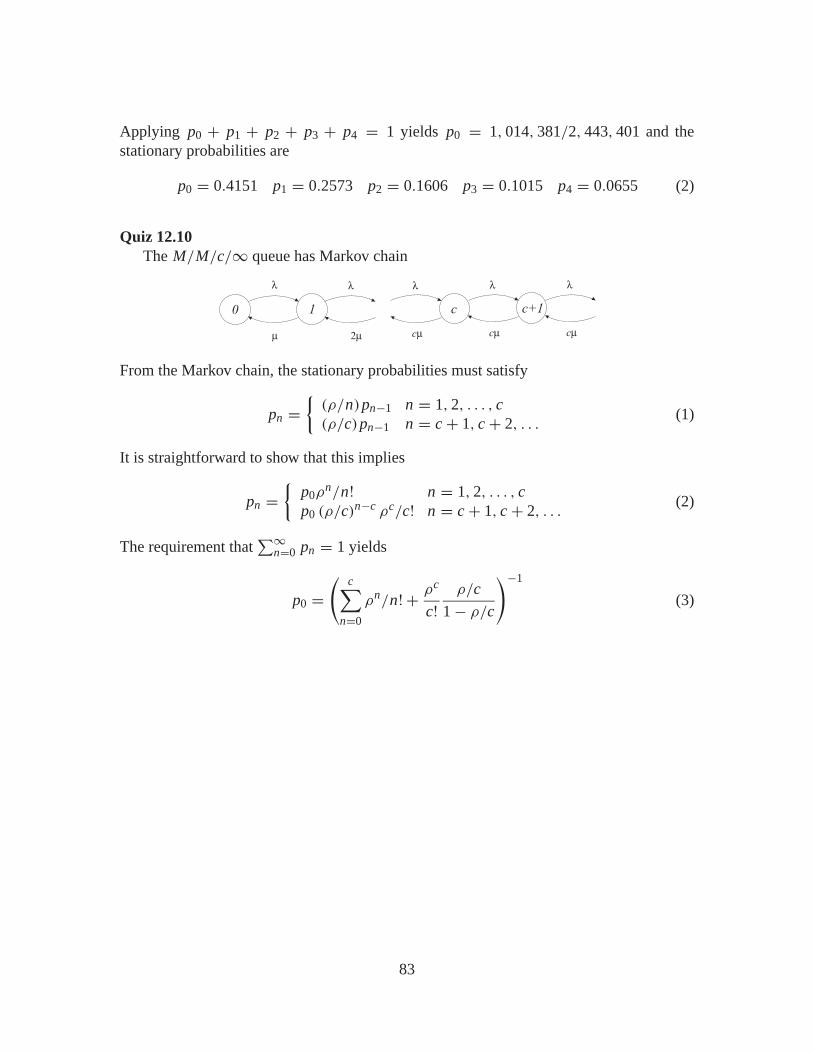
Applying p0 + p1 + p2 + p3 + p4 = 1 yields p0 = 1, 014, 381/2, 443, 401 and thestationary probabilities are
p0 = 0.4151 p1 = 0.2573 p2 = 0.1606 p3 = 0.1015 p4 = 0.0655 (2)
Quiz 12.10The M/M/c/∞ queue has Markov chain
c c+110
λ λ λ λ λ
µ 2µ cµ cµ cµ
From the Markov chain, the stationary probabilities must satisfy
pn ={
(ρ/n)pn−1 n = 1, 2, . . . , c(ρ/c)pn−1 n = c + 1, c + 2, . . .
(1)
It is straightforward to show that this implies
pn ={
p0ρn/n! n = 1, 2, . . . , c
p0 (ρ/c)n−c ρc/c! n = c + 1, c + 2, . . .(2)
The requirement that∑∞
n=0 pn = 1 yields
p0 =(
c∑n=0
ρn/n! + ρc
c!ρ/c
1− ρ/c
)−1
(3)
83