probability and stochastic processes with...
TRANSCRIPT

Probability and Stochastic Processes
with Applications
Oliver Knill

Contents
Preface 3
1 Introduction 51.1 What is probability theory? . . . . . . . . . . . . . . . . . . 51.2 Some paradoxes in probability theory . . . . . . . . . . . . 121.3 Some applications of probability theory . . . . . . . . . . . 16
2 Limit theorems 232.1 Probability spaces, random variables, independence . . . . . 232.2 Kolmogorov’s 0 − 1 law, Borel-Cantelli lemma . . . . . . . . 342.3 Integration, Expectation, Variance . . . . . . . . . . . . . . 392.4 Results from real analysis . . . . . . . . . . . . . . . . . . . 422.5 Some inequalities . . . . . . . . . . . . . . . . . . . . . . . . 442.6 The weak law of large numbers . . . . . . . . . . . . . . . . 502.7 The probability distribution function . . . . . . . . . . . . . 562.8 Convergence of random variables . . . . . . . . . . . . . . . 592.9 The strong law of large numbers . . . . . . . . . . . . . . . 642.10 Birkhoff’s ergodic theorem . . . . . . . . . . . . . . . . . . . 682.11 More convergence results . . . . . . . . . . . . . . . . . . . . 722.12 Classes of random variables . . . . . . . . . . . . . . . . . . 782.13 Weak convergence . . . . . . . . . . . . . . . . . . . . . . . 902.14 The central limit theorem . . . . . . . . . . . . . . . . . . . 922.15 Entropy of distributions . . . . . . . . . . . . . . . . . . . . 982.16 Markov operators . . . . . . . . . . . . . . . . . . . . . . . . 1072.17 Characteristic functions . . . . . . . . . . . . . . . . . . . . 1102.18 The law of the iterated logarithm . . . . . . . . . . . . . . . 117
3 Discrete Stochastic Processes 1233.1 Conditional Expectation . . . . . . . . . . . . . . . . . . . . 1233.2 Martingales . . . . . . . . . . . . . . . . . . . . . . . . . . . 1313.3 Doob’s convergence theorem . . . . . . . . . . . . . . . . . . 1433.4 Levy’s upward and downward theorems . . . . . . . . . . . 1503.5 Doob’s decomposition of a stochastic process . . . . . . . . 1523.6 Doob’s submartingale inequality . . . . . . . . . . . . . . . 1573.7 Doob’s Lp inequality . . . . . . . . . . . . . . . . . . . . . . 1593.8 Random walks . . . . . . . . . . . . . . . . . . . . . . . . . 162
1

2 Contents
3.9 The arc-sin law for the 1D random walk . . . . . . . . . . . 1673.10 The random walk on the free group . . . . . . . . . . . . . . 1713.11 The free Laplacian on a discrete group . . . . . . . . . . . . 1753.12 A discrete Feynman-Kac formula . . . . . . . . . . . . . . . 1793.13 Discrete Dirichlet problem . . . . . . . . . . . . . . . . . . . 1813.14 Markov processes . . . . . . . . . . . . . . . . . . . . . . . . 186
4 Continuous Stochastic Processes 1914.1 Brownian motion . . . . . . . . . . . . . . . . . . . . . . . . 1914.2 Some properties of Brownian motion . . . . . . . . . . . . . 1984.3 The Wiener measure . . . . . . . . . . . . . . . . . . . . . . 2054.4 Levy’s modulus of continuity . . . . . . . . . . . . . . . . . 2074.5 Stopping times . . . . . . . . . . . . . . . . . . . . . . . . . 2094.6 Continuous time martingales . . . . . . . . . . . . . . . . . 2154.7 Doob inequalities . . . . . . . . . . . . . . . . . . . . . . . . 2174.8 Khintchine’s law of the iterated logarithm . . . . . . . . . . 2194.9 The theorem of Dynkin-Hunt . . . . . . . . . . . . . . . . . 2224.10 Self-intersection of Brownian motion . . . . . . . . . . . . . 2234.11 Recurrence of Brownian motion . . . . . . . . . . . . . . . . 2284.12 Feynman-Kac formula . . . . . . . . . . . . . . . . . . . . . 2304.13 The quantum mechanical oscillator . . . . . . . . . . . . . . 2354.14 Feynman-Kac for the oscillator . . . . . . . . . . . . . . . . 2384.15 Neighborhood of Brownian motion . . . . . . . . . . . . . . 2414.16 The Ito integral for Brownian motion . . . . . . . . . . . . . 2454.17 Processes of bounded quadratic variation . . . . . . . . . . 2554.18 The Ito integral for martingales . . . . . . . . . . . . . . . . 2604.19 Stochastic differential equations . . . . . . . . . . . . . . . . 264
5 Selected Topics 2755.1 Percolation . . . . . . . . . . . . . . . . . . . . . . . . . . . 2755.2 Random Jacobi matrices . . . . . . . . . . . . . . . . . . . . 2865.3 Estimation theory . . . . . . . . . . . . . . . . . . . . . . . 2925.4 Vlasov dynamics . . . . . . . . . . . . . . . . . . . . . . . . 2985.5 Multidimensional distributions . . . . . . . . . . . . . . . . 3065.6 Poisson processes . . . . . . . . . . . . . . . . . . . . . . . . 3115.7 Random maps . . . . . . . . . . . . . . . . . . . . . . . . . . 3165.8 Circular random variables . . . . . . . . . . . . . . . . . . . 3195.9 Lattice points near Brownian paths . . . . . . . . . . . . . . 3275.10 Arithmetic random variables . . . . . . . . . . . . . . . . . 3335.11 Symmetric Diophantine Equations . . . . . . . . . . . . . . 3435.12 Continuity of random variables . . . . . . . . . . . . . . . . 349

Preface
These notes grew from an introduction to probability theory taught duringthe first and second term of 1994 at Caltech. There was a mixed audience ofundergraduates and graduate students in the first half of the course whichcovered Chapters 2 and 3, and mostly graduate students in the second partwhich covered Chapter 4 and two sections of Chapter 5.
Having been online for many years on my personal web sites, the text gotreviewed, corrected and indexed in the summer of 2006. It obtained someenhancements which benefited from some other teaching notes and research,I wrote while teaching probability theory at the University of Arizona inTucson or when incorporating probability in calculus courses at Caltechand Harvard University.
Most of Chapter 2 is standard material and subject of virtually any courseon probability theory. Also Chapters 3 and 4 is well covered by the litera-ture but not in this combination.
The last chapter ”selected topics” got considerably extended in the summerof 2006. While in the original course, only localization and percolation prob-lems were included, I added other topics like estimation theory, Vlasov dy-namics, multi-dimensional moment problems, random maps, circle-valuedrandom variables, the geometry of numbers, Diophantine equations andharmonic analysis. Some of this material is related to research I got inter-ested in over time.
While the text assumes no prerequisites in probability, a basic exposure tocalculus and linear algebra is necessary. Some real analysis as well as somebackground in topology and functional analysis can be helpful.
I would like to get feedback from readers. I plan to keep this text alive andupdate it in the future. You can email this to [email protected] andalso indicate on the email if you don’t want your feedback to be acknowl-edged in an eventual future edition of these notes.
3

4 Contents
To get a more detailed and analytic exposure to probability, the studentsof the original course have consulted the book [105] which contains muchmore material than covered in class. Since my course had been taught,many other books have appeared. Examples are [21, 34].
For a less analytic approach, see [40, 91, 97] or the still excellent classic[26]. For an introduction to martingales, we recommend [108] and [47] fromboth of which these notes have benefited a lot and to which the studentsof the original course had access too.
For Brownian motion, we refer to [73, 66], for stochastic processes to [17],for stochastic differential equation to [2, 55, 76, 66, 46], for random walksto [100], for Markov chains to [27, 87], for entropy and Markov operators[61]. For applications in physics and chemistry, see [106].
For the selected topics, we followed [32] in the percolation section. Thebooks [101, 30] contain introductions to Vlasov dynamics. The book of [1]gives an introduction for the moment problem, [75, 64] for circle-valuedrandom variables, for Poisson processes, see [49, 9]. For the geometry ofnumbers for Fourier series on fractals [45].
The book [109] contains examples which challenge the theory with counterexamples. [33, 92, 70] are sources for problems with solutions.
Probability theory can be developed using nonstandard analysis on finiteprobability spaces [74]. The book [42] breaks some of the material of thefirst chapter into attractive stories. Also texts like [89, 78] are not only formathematical tourists.
We live in a time, in which more and more content is available online.Knowledge diffuses from papers and books to online websites and databaseswhich also ease the digging for knowledge in the fascinating field of proba-bility theory.
Oliver Knill, March 20, 2008

Chapter 1
Introduction
1.1 What is probability theory?
Probability theory is a fundamental pillar of modern mathematics withrelations to other mathematical areas like algebra, topology, analysis, ge-ometry or dynamical systems. As with any fundamental mathematical con-struction, the theory starts by adding more structure to a set Ω. In a similarway as introducing algebraic operations, a topology, or a time evolution ona set, probability theory adds a measure theoretical structure to Ω whichgeneralizes ”counting” on finite sets: in order to measure the probabilityof a subset A ⊂ Ω, one singles out a class of subsets A, on which one canhope to do so. This leads to the notion of a σ-algebra A. It is a set of sub-sets of Ω in which on can perform finitely or countably many operationslike taking unions, complements or intersections. The elements in A arecalled events. If a point ω in the ”laboratory” Ω denotes an ”experiment”,an ”event” A ∈ A is a subset of Ω, for which one can assign a proba-bility P[A] ∈ [0, 1]. For example, if P[A] = 1/3, the event happens withprobability 1/3. If P[A] = 1, the event takes place almost certainly. Theprobability measure P has to satisfy obvious properties like that the unionA ∪B of two disjoint events A,B satisfies P[A ∪B] = P[A] + P[B] or thatthe complement Ac of an event A has the probability P[Ac] = 1 − P[A].With a probability space (Ω,A,P) alone, there is already some interestingmathematics: one has for example the combinatorial problem to find theprobabilities of events like the event to get a ”royal flush” in poker. If Ωis a subset of an Euclidean space like the plane, P[A] =
∫
A f(x, y) dxdyfor a suitable nonnegative function f , we are led to integration problemsin calculus. Actually, in many applications, the probability space is part ofEuclidean space and the σ-algebra is the smallest which contains all opensets. It is called the Borel σ-algebra. An important example is the Borelσ-algebra on the real line.
Given a probability space (Ω,A,P), one can define random variables X . Arandom variable is a function X from Ω to the real line R which is mea-surable in the sense that the inverse of a measurable Borel set B in R is
5

6 Chapter 1. Introduction
in A. The interpretation is that if ω is an experiment, then X(ω) mea-sures an observable quantity of the experiment. The technical condition ofmeasurability resembles the notion of a continuity for a function f from atopological space (Ω,O) to the topological space (R,U). A function is con-tinuous if f−1(U) ∈ O for all open sets U ∈ U . In probability theory, wherefunctions are often denoted with capital letters, like X,Y, . . . , a randomvariable X is measurable if X−1(B) ∈ A for all Borel sets B ∈ B. Anycontinuous function is measurable for the Borel σ-algebra. As in calculus,where one does not have to worry about continuity most of the time, also inprobability theory, one often does not have to sweat about measurability is-sues. Indeed, one could suspect that notions like σ-algebras or measurabilitywere introduced by mathematicians to scare normal folks away from theirrealms. This is not the case. Serious issues are avoided with those construc-tions. Mathematics is eternal: a once established result will be true also inthousands of years. A theory in which one could prove a theorem as well asits negation would be worthless: it would formally allow to prove any otherresult, whether true or false. So, these notions are not only introduced tokeep the theory ”clean”, they are essential for the ”survival” of the theory.We give some examples of ”paradoxes” to illustrate the need for buildinga careful theory. Back to the fundamental notion of random variables: be-cause they are just functions, one can add and multiply them by defining(X + Y )(ω) = X(ω) + Y (ω) or (XY )(ω) = X(ω)Y (ω). Random variablesform so an algebra L. The expectation of a random variable X is denotedby E[X ] if it exists. It is a real number which indicates the ”mean” or ”av-erage” of the observationX . It is the value, one would expect to measure inthe experiment. If X = 1B is the random variable which has the value 1 ifω is in the event B and 0 if ω is not in the event B, then the expectation ofX is just the probability of B. The constant random variable X(ω) = a hasthe expectation E[X ] = a. These two basic examples as well as the linearityrequirement E[aX+ bY ] = aE[X ]+ bE[Y ] determine the expectation for allrandom variables in the algebra L: first one defines expectation for finitesums
∑ni=1 ai1Bi called elementary random variables, which approximate
general measurable functions. Extending the expectation to a subset L1 ofthe entire algebra is part of integration theory. While in calculus, one canlive with the Riemann integral on the real line, which defines the integral
by Riemann sums∫ b
a f(x) dx ∼ 1n
∑
i/n∈[a,b] f(i/n), the integral defined inmeasure theory is the Lebesgue integral. The later is more fundamentaland probability theory is a major motivator for using it. It allows to makestatements like that the probability of the set of real numbers with periodicdecimal expansion has probability 0. In general, the probability of A is theexpectation of the random variable X(x) = f(x) = 1A(x). In calculus, the
integral∫ 1
0 f(x) dx would not be defined because a Riemann integral cangive 1 or 0 depending on how the Riemann approximation is done. Probabil-
ity theory allows to introduce the Lebesgue integral by defining∫ b
af(x) dx
as the limit of 1n
∑ni=1 f(xi) for n → ∞, where xi are random uniformly
distributed points in the interval [a, b]. This Monte Carlo definition of theLebesgue integral is based on the law of large numbers and is as intuitive

1.1. What is probability theory? 7
to state as the Riemann integral which is the limit of 1n
∑
xj=j/n∈[a,b] f(xj)for n→ ∞.
With the fundamental notion of expectation one can define the variance,Var[X ] = E[X2]−E[X ]2 and the standard deviation σ[X ] =
√
Var[X ] of arandom variable X for which X2 ∈ L1. One can also look at the covarianceCov[XY ] = E[XY ] − E[X ]E[Y ] of two random variables X,Y for whichX2, Y 2 ∈ L1. The correlation Corr[X,Y ] = Cov[XY ]/(σ[X ]σ[Y ]) of tworandom variables with positive variance is a number which tells how muchthe random variable X is related to the random variable Y . If E[XY ] isinterpreted as an inner product, then the standard deviation is the lengthof X−E[X ] and the correlation has the geometric interpretation as cos(α),where α is the angle between the centered random variables X −E[X ] andY − E[Y ]. For example, if Cov[X,Y ] = 1, then Y = λX for some λ > 0, ifCov[X,Y ] = −1, they are anti-parallel. If the correlation is zero, the geo-metric interpretation is that the two random variables are perpendicular.Decorrelated random variables still can have relations to each other but iffor any measurable real functions f and g, the random variables f(X) andg(X) are uncorrelated, then the random variables X,Y are independent.
A random variable X can be described well by its distribution functionFX . This is a real-valued function defined as FX(s) = P[X ≤ s] on R,where X ≤ s is the event of all experiments ω satisfying X(ω) ≤ s. Thedistribution function does not encode the internal structure of the randomvariable X ; it does not reveal the structure of the probability space for ex-ample. But the function FX allows the construction of a probability spacewith exactly this distribution function. There are two important types ofdistributions, continuous distributions with a probability density functionfX = F ′
X and discrete distributions for which F is piecewise constant. Anexample of a continuous distribution is the standard normal distribution,where fX(x) = e−x
2/2/√
2π. One can characterize it as the distributionwith maximal entropy I(f) = −
∫
log(f(x))f(x) dx among all distributionswhich have zero mean and variance 1. An example of a discrete distribu-
tion is the Poisson distribution P[X = k] = e−λ λk
k! on N = 0, 1, 2, . . . .One can describe random variables by their moment generating functionsMX(t) = E[eXt] or by their characteristic function φX(t) = E[eiXt]. Thelater is the Fourier transform of the law µX = F ′
X which is a measure onthe real line R.
The law µX of the random variable is a probability measure on the realline satisfying µX((a, b]) = FX(b)−FX(a). By the Lebesgue decompositiontheorem, one can decompose any measure µ into a discrete part µpp, anabsolutely continuous part µac and a singular continuous part µsc. Randomvariables X for which µX is a discrete measure are called discrete randomvariables, random variables with a continuous law are called continuousrandom variables. Traditionally, these two type of random variables arethe most important ones. But singular continuous random variables appeartoo: in spectral theory, dynamical systems or fractal geometry. Of course,the law of a random variable X does not need to be pure. It can mix the

8 Chapter 1. Introduction
three types. A random variable can be mixed discrete and continuous forexample.
Inequalities play an important role in probability theory. The Chebychev
inequality P[|X − E[X ]| ≥ c] ≤ Var[X]c2 is used very often. It is a spe-
cial case of the Chebychev-Markov inequality h(c) · P[X ≥ c] ≤ E[h(X)]for monotone nonnegative functions h. Other inequalities are the Jenseninequality E[h(X)] ≥ h(E[X ]) for convex functions h, the Minkowski in-equality ||X + Y ||p ≤ ||X ||p + ||Y ||p or the Holder inequality ||XY ||1 ≤||X ||p||Y ||q, 1/p + 1/q = 1 for random variables, X,Y , for which ||X ||p =E[|X |p], ||Y ||q = E[|Y |q] are finite. Any inequality which appears in analy-sis can be useful in the toolbox of probability theory.
Independence is an central notion in probability theory. Two events A,Bare called independent, if P[A ∩ B] = P[A] · P[B]. An arbitrary set ofevents Ai is called independent, if for any finite subset of them, the prob-ability of their intersection is the product of their probabilities. Two σ-algebras A,B are called independent, if for any pair A ∈ A, B ∈ B, theevents A,B are independent. Two random variables X,Y are independent,if they generate independent σ-algebras. It is enough to check that theevents A = X ∈ (a, b) and B = Y ∈ (c, d) are independent forall intervals (a, b) and (c, d). One should think of independent randomvariables as two aspects of the laboratory Ω which do not influence eachother. Each event A = a < X(ω) < b is independent of the eventB = c < Y (ω) < d . While the distribution function FX+Y of the sum oftwo independent random variables is a convolution
∫
RFX(t−s) dFY (s), the
moment generating functions and characteristic functions satisfy the for-mulas MX+Y (t) = MX(t)MY (t) and φX+Y (t) = φX(t)φY (t). These identi-ties makeMX , φX valuable tools to compute the distribution of an arbitraryfinite sum of independent random variables.
Independence can also be explained using conditional probability with re-spect to an event B of positive probability: the conditional probabilityP[A|B] = P[A ∩ B]/P[B] of A is the probability that A happens when weknow that B takes place. If B is independent of A, then P[A|B] = P[A] butin general, the conditional probability is larger. The notion of conditionalprobability leads to the important notion of conditional expectation E[X |B]of a random variable X with respect to some sub-σ-algebra B of the σ al-gebra A; it is a new random variable which is B-measurable. For B = A, itis the random variable itself, for the trivial algebra B = ∅,Ω , we obtainthe usual expectation E[X ] = E[X |∅,Ω ]. If B is generated by a finitepartition B1, . . . , Bn of Ω of pairwise disjoint sets covering Ω, then E[X |B]is piecewise constant on the sets Bi and the value on Bi is the averagevalue of X on Bi. If B is the σ-algebra of an independent random variableY , then E[X |Y ] = E[X |B] = E[X ]. In general, the conditional expectationwith respect to B is a new random variable obtained by averaging on theelements of B. One has E[X |Y ] = h(Y ) for some function h, extreme casesbeing E[X |1] = E[X ],E[X |X ] = X . An illustrative example is the situation

1.1. What is probability theory? 9
where X(x, y) is a continuous function on the unit square with P = dxdyas a probability measure and where Y (x, y) = x. In that case, E[X |Y ] is
a function of x alone, given by E[X |Y ](x) =∫ 1
0 f(x, y) dy. This is called aconditional integral.
A set Xtt∈T of random variables defines a stochastic process. The vari-able t ∈ T is a parameter called ”time”. Stochastic processes are to prob-ability theory what differential equations are to calculus. An example is afamily Xn of random variables which evolve with discrete time n ∈ N. De-terministic dynamical system theory branches into discrete time systems,the iteration of maps and continuous time systems, the theory of ordinaryand partial differential equations. Similarly, in probability theory, one dis-tinguishes between discrete time stochastic processes and continuous timestochastic processes. A discrete time stochastic process is a sequence of ran-dom variables Xn with certain properties. An important example is whenXn are independent, identically distributed random variables. A continuoustime stochastic process is given by a family of random variables Xt, wheret is real time. An example is a solution of a stochastic differential equation.With more general time like Zd or Rd random variables are called randomfields which play a role in statistical physics. Examples of such processesare percolation processes.
While one can realize every discrete time stochastic processXn by a measure-preserving transformation T : Ω → Ω and Xn(ω) = X(T n(ω)), probabil-ity theory often focuses a special subclass of systems called martingales,where one has a filtration An ⊂ An+1 of σ-algebras such that Xn is An-measurable and E[Xn|An−1] = Xn−1, where E[Xn|An−1] is the conditionalexpectation with respect to the sub-algebra An−1. Martingales are a pow-erful generalization of the random walk, the process of summing up IIDrandom variables with zero mean. Similar as ergodic theory, martingaletheory is a natural extension of probability theory and has many applica-tions.
The language of probability fits well into the classical theory of dynam-ical systems. For example, the ergodic theorem of Birkhoff for measure-preserving transformations has as a special case the law of large numberswhich describes the average of partial sums of random variables 1
n
∑mk=1Xk.
There are different versions of the law of large numbers. ”Weak laws”make statements about convergence in probability, ”strong laws” makestatements about almost everywhere convergence. There are versions ofthe law of large numbers for which the random variables do not need tohave a common distribution and which go beyond Birkhoff’s theorem. Another important theorem is the central limit theorem which shows thatSn = X1 + X2 + · · · + Xn normalized to have zero mean and variance 1converges in law to the normal distribution or the law of the iterated loga-rithm which says that for centered independent and identically distributedXk, the scaled sum Sn/Λn has accumulation points in the interval [−σ, σ]if Λn =
√2n log logn and σ is the standard deviation of Xk. While stating

10 Chapter 1. Introduction
the weak and strong law of large numbers and the central limit theorem,different convergence notions for random variables appear: almost sure con-vergence is the strongest, it implies convergence in probability and the laterimplies convergence convergence in law. There is also L1-convergence whichis stronger than convergence in probability.
As in the deterministic case, where the theory of differential equations ismore technical than the theory of maps, building up the formalism forcontinuous time stochastic processes Xt is more elaborate. Similarly asfor differential equations, one has first to prove the existence of the ob-jects. The most important continuous time stochastic process definitely isBrownian motion Bt. Standard Brownian motion is a stochastic processwhich satisfies B0 = 0, E[Bt] = 0, Cov[Bs, Bt] = s for s ≤ t and forany sequence of times, 0 = t0 < t1 < · · · < ti < ti+1, the incrementsBti+1 − Bti are all independent random vectors with normal distribution.Brownian motion Bt is a solution of the stochastic differential equationddtBt = ζ(t), where ζ(t) is called white noise. Because white noise is onlydefined as a generalized function and is not a stochastic process by itself,this stochastic differential equation has to be understood in its integratedform Bt =
∫ t
0 dBs =∫ t
0 ζ(s) ds.
More generally, a solution to a stochastic differential equation ddtXt =
f(Xt)ζ(t) + g(Xt) is defined as the solution to the integral equation Xt =
X0 +∫ t
0 f(Xs) dBt +∫ t
0 g(Xs) ds. Stochastic differential equations can
be defined in different ways. The expression∫ t
0f(Xs) dBt can either be
defined as an Ito integral, which leads to martingale solutions, or theStratonovich integral, which has similar integration rules than classicaldifferentiation equations. Examples of stochastic differential equations areddtXt = Xtζ(t) which has the solution Xt = eBt−t/2. Or d
dtXt = B4t ζ(t)
which has as the solution the process Xt = B5t −10B3
t +15Bt. The key toolto solve stochastic differential equations is Ito’s formula f(Bt) − f(B0) =∫ t
0f ′(Bs)dBs + 1
2
∫ t
0f ′′(Bs) ds, which is the stochastic analog of the fun-
damental theorem of calculus. Solutions to stochastic differential equationsare examples of Markov processes which show diffusion. Especially, the so-lutions can be used to solve classical partial differential equations like theDirichlet problem ∆u = 0 in a bounded domain D with u = f on theboundary δD. One can get the solution by computing the expectation off at the end points of Brownian motion starting at x and ending at theboundary u = Ex[f(BT )]. On a discrete graph, if Brownian motion is re-placed by random walk, the same formula holds too. Stochastic calculus isalso useful to interpret quantum mechanics as a diffusion processes [73, 71]or as a tool to compute solutions to quantum mechanical problems usingFeynman-Kac formulas.
Some features of stochastic process can be described using the language ofMarkov operators P , which are positive and expectation-preserving trans-formations on L1. Examples of such operators are Perron-Frobenius op-erators X → X(T ) for a measure preserving transformation T defining a

1.1. What is probability theory? 11
discrete time evolution or stochastic matrices describing a random walkon a finite graph. Markov operators can be defined by transition proba-bility functions which are measure-valued random variables. The interpre-tation is that from a given point ω, there are different possibilities to goto. A transition probability measure P(ω, ·) gives the distribution of thetarget. The relation with Markov operators is assured by the Chapman-Kolmogorov equation Pn+m = Pn Pm. Markov processes can be obtainedfrom random transformations, random walks or by stochastic differentialequations. In the case of a finite or countable target space S, one obtainsMarkov chains which can be described by probability matrices P , whichare the simplest Markov operators. For Markov operators, there is an ar-row of time: the relative entropy with respect to a background measureis non-increasing. Markov processes often are attracted by fixed points ofthe Markov operator. Such fixed points are called stationary states. Theydescribe equilibria and often they are measures with maximal entropy. Anexample is the Markov operator P , which assigns to a probability densityfY the probability density of fY+X where Y +X is the random variableY + X normalized so that it has mean 0 and variance 1. For the initialfunction f = 1, the function Pn(fX) is the distribution of S∗
n the nor-malized sum of n IID random variables Xi. This Markov operator has aunique equilibrium point, the standard normal distribution. It has maxi-mal entropy among all distributions on the real line with variance 1 andmean 0. The central limit theorem tells that the Markov operator P hasthe normal distribution as a unique attracting fixed point if one takes theweaker topology of convergence in distribution on L1. This works in othersituations too. For circle-valued random variables for example, the uniformdistribution maximizes entropy. It is not surprising therefore, that there isa central limit theorem for circle-valued random variables with the uniformdistribution as the limiting distribution.
In the same way as mathematics reaches out into other scientific areas,probability theory has connections with many other branches of mathe-matics. The last chapter of these notes give some examples. The sectionon percolation shows how probability theory can help to understand criti-cal phenomena. In solid state physics, one considers operator-valued ran-dom variables. The spectrum of random operators are random objects too.One is interested what happens with probability one. Localization is thephenomenon in solid state physics that sufficiently random operators of-ten have pure point spectrum. The section on estimation theory gives aglimpse of what mathematical statistics is about. In statistics one oftendoes not know the probability space itself so that one has to make a statis-tical model and look at a parameterization of probability spaces. The goalis to give maximum likelihood estimates for the parameters from data andto understand how small the quadratic estimation error can be made. Asection on Vlasov dynamics shows how probability theory appears in prob-lems of geometric evolution. Vlasov dynamics is a generalization of then-body problem to the evolution of of probability measures. One can lookat the evolution of smooth measures or measures located on surfaces. This

12 Chapter 1. Introduction
deterministic stochastic system produces an evolution of densities whichcan form singularities without doing harm to the formalism. It also definesthe evolution of surfaces. The section on moment problems is part of multi-variate statistics. As for random variables, random vectors can be describedby their moments. Since moments define the law of the random variable,the question arises how one can see from the moments, whether we have acontinuous random variable. The section of random maps is an other partof dynamical systems theory. Randomized versions of diffeomorphisms canbe considered idealization of their undisturbed versions. They often canbe understood better than their deterministic versions. For example, manyrandom diffeomorphisms have only finitely many ergodic components. Inthe section in circular random variables, we see that the Mises distribu-tion has extremal entropy among all circle-valued random variables withgiven circular mean and variance. There is also a central limit theoremon the circle: the sum of IID circular random variables converges in lawto the uniform distribution. We then look at a problem in the geometryof numbers: how many lattice points are there in a neighborhood of thegraph of one-dimensional Brownian motion? The analysis of this problemneeds a law of large numbers for independent random variables Xk withuniform distribution on [0, 1]: for 0 ≤ δ < 1, and An = [0, 1/nδ] one has
limn→∞1n
∑nk=1
1An (Xk)nδ = 1. Probability theory also matters in complex-
ity theory as a section on arithmetic random variables shows. It turns outthat random variables like Xn(k) = k, Yn(k) = k2 + 3 mod n defined onfinite probability spaces become independent in the limit n → ∞. Suchconsiderations matter in complexity theory: arithmetic functions definedon large but finite sets behave very much like random functions. This isreflected by the fact that the inverse of arithmetic functions is in generaldifficult to compute and belong to the complexity class of NP. Indeed, ifone could invert arithmetic functions easily, one could solve problems likefactoring integers fast. A short section on Diophantine equations indicateshow the distribution of random variables can shed light on the solutionof Diophantine equations. Finally, we look at a topic in harmonic analy-sis which was initiated by Norbert Wiener. It deals with the relation ofthe characteristic function φX and the continuity properties of the randomvariable X .
1.2 Some paradoxes in probability theory
Colloquial language is not always precise enough to tackle problems inprobability theory. Paradoxes appear, when definitions allow different in-terpretations. Ambiguous language can lead to wrong conclusions or con-tradicting solutions. To illustrate this, we mention a few problems. Thefollowing four examples should serve as a motivation to introduce proba-bility theory on a rigorous mathematical footing.
1) Bertrand’s paradox (Bertrand 1889)We throw at random lines onto the unit disc. What is the probability that

1.2. Some paradoxes in probability theory 13
the line intersects the disc with a length ≥√
3, the length of the inscribedequilateral triangle?
First answer: take an arbitrary point P on the boundary of the disc. Theset of all lines through that point are parameterized by an angle φ. In orderthat the chord is longer than
√3, the line has to lie within a sector of 60
within a range of 180. The probability is 1/3.
Second answer: take all lines perpendicular to a fixed diameter. The chordis longer than
√3 if the point of intersection lies on the middle half of the
diameter. The probability is 1/2.
Third answer: if the midpoints of the chords lie in a disc of radius 1/2, thechord is longer than
√3. Because the disc has a radius which is half the
radius of the unit disc, the probability is 1/4.
Figure. Random an-gle.
Figure. Randomtranslation.
Figure. Random area.
Like most paradoxes in mathematics, a part of the question in Bertrand’sproblem is not well defined. Here it is the term ”random line”. The solu-tion of the paradox lies in the fact that the three answers depend on thechosen probability distribution. There are several ”natural” distributions.The actual answer depends on how the experiment is performed.
2) Petersburg paradox (D.Bernoulli, 1738)In the Petersburg casino, you pay an entrance fee c and you get the prize2T , where T is the number of times, the casino flips a coin until ”head”appears. For example, if the sequence of coin experiments would give ”tail,tail, tail, head”, you would win 23 − c = 8 − c, the win minus the entrancefee. Fair would be an entrance fee which is equal to the expectation of thewin, which is
∞∑
k=1
2kP[T = k] =
∞∑
k=1
1 = ∞ .
The paradox is that nobody would agree to pay even an entrance fee c = 10.

14 Chapter 1. Introduction
The problem with this casino is that it is not quite clear, what is ”fair”.For example, the situation T = 20 is so improbable that it never occursin the life-time of a person. Therefore, for any practical reason, one hasnot to worry about large values of T . This, as well as the finiteness ofmoney resources is the reason, why casinos do not have to worry about thefollowing bullet proof martingale strategy in roulette: bet c dollars on red.If you win, stop, if you lose, bet 2c dollars on red. If you win, stop. If youlose, bet 4c dollars on red. Keep doubling the bet. Eventually after n steps,red will occur and you will win 2nc − (c + 2c + · · · + 2n−1c) = c dollars.This example motivates the concept of martingales. Theorem (3.2.7) orproposition (3.2.9) will shed some light on this. Back to the Petersburgparadox. How does one resolve it? What would be a reasonable entrancefee in ”real life”? Bernoulli proposed to replace the expectation E[G] of theprofit G = 2T with the expectation (E[
√G])2, where u(x) =
√x is called a
utility function. This would lead to a fair entrance
(E[√G])2 = (
∞∑
k=1
2k/22−k)2 =1
(√
2 − 1)2∼ 5.828... .
It is not so clear if that is a way out of the paradox because for any proposedutility function u(k), one can modify the casino rule so that the paradox
reappears: pay (2k)2 if the utility function u(k) =√k or pay e2
k
dollars,if the utility function is u(k) = log(k). Such reasoning plays a role ineconomics and social sciences.
Figure. The picture to the rightshows the average profit devel-opment during a typical tourna-ment of 4000 Petersburg games.After these 4000 games, theplayer would have lost about 10thousand dollars, when paying a10 dollar entrance fee each game.The player would have to play avery, very long time to catch up.Mathematically, the player willdo so and have a profit in thelong run, but it is unlikely thatit will happen in his or her lifetime.
1000 2000 3000 4000
4
6
8
3) The three door problem (1991) Suppose you’re on a game show andyou are given a choice of three doors. Behind one door is a car and behindthe others are goats. You pick a door-say No. 1 - and the host, who knowswhat’s behind the doors, opens another door-say, No. 3-which has a goat.(In all games, he opens a door to reveal a goat). He then says to you, ”Do

1.2. Some paradoxes in probability theory 15
you want to pick door No. 2?” (In all games he always offers an option toswitch). Is it to your advantage to switch your choice?
The problem is also called ”Monty Hall problem” and was discussed byMarilyn vos Savant in a ”Parade” column in 1991 and provoked a bigcontroversy. (See [98] for pointers and similar examples.) The problem isthat intuitive argumentation can easily lead to the conclusion that it doesnot matter whether to change the door or not. Switching the door doublesthe chances to win:
No switching: you choose a door and win with probability 1/3. The openingof the host does not affect any more your choice.Switching: when choosing the door with the car, you loose since you switch.If you choose a door with a goat. The host opens the other door with thegoat and you win. There are two such cases, where you win. The probabilityto win is 2/3.
4) The Banach-Tarski paradox (1924)It is possible to cut the standard unit ball Ω = x ∈ R3 | |x| ≤ 1 into 5disjoint pieces Ω = Y1∪Y2∪Y3∪Y4∪Y5 and rotate and translate the pieceswith transformations Ti so that T1(Y1)∪T2(Y2) = Ω and T3(Y3)∪T4(Y4)∪T5(Y5) = Ω′ is a second unit ball Ω′ = x ∈ R3 | |x− (3, 0, 0)| ≤ 1 and allthe transformed sets again don’t intersect.While this example of Banach-Tarski is spectacular, the existence of boundedsubsets A of the circle for which one can not assign a translational invari-ant probability P[A] can already be achieved in one dimension. The Italianmathematician Giuseppe Vitali gave in 1905 the following example: definean equivalence relation on the circle T = [0, 2π) by saying that two anglesare equivalent x ∼ y if (x−y)/π is a rational angle. Let A be a subset in thecircle which contains exactly one number from each equivalence class. Theaxiom of choice assures the existence of A. If x1, x2, . . . is a enumerationof the set of rational angles in the circle, then the sets Ai = A + xi arepairwise disjoint and satisfy
⋃∞i=1 Ai = T. If we could assign a translational
invariant probability P[Ai] to A, then the basic rules of probability wouldgive
1 = P[T] = P[
∞⋃
i=1
Ai] =
∞∑
i=1
P[Ai] =
∞∑
i=1
p .
But there is no real number p = P[A] = P[Ai] which makes this possible.Both the Banach-Tarski as well as Vitalis result shows that one can nothope to define a probability space on the algebra A of all subsets of the unitball or the unit circle such that the probability measure is translationaland rotational invariant. The natural concepts of ”length” or ”volume”,which are rotational and translational invariant only makes sense for asmaller algebra. This will lead to the notion of σ-algebra. In the contextof topological spaces like Euclidean spaces, it leads to Borel σ-algebras,algebras of sets generated by the compact sets of the topological space.This language will be developed in the next chapter.

16 Chapter 1. Introduction
1.3 Some applications of probability theory
Probability theory is a central topic in mathematics. There are close re-lations and intersections with other fields like computer science, ergodictheory and dynamical systems, cryptology, game theory, analysis, partialdifferential equation, mathematical physics, economical sciences, statisticalmechanics and even number theory. As a motivation, we give some prob-lems and topics which can be treated with probabilistic methods.
1) Random walks: (statistical mechanics, gambling, stock markets, quan-tum field theory).
Assume you walk through a lattice. At each vertex, you choose a directionat random. What is the probability that you return back to your start-ing point? Polya’s theorem (3.8.1) says that in two dimensions, a randomwalker almost certainly returns to the origin arbitrarily often, while in threedimensions, the walker with probability 1 only returns a finite number oftimes and then escapes for ever.
Figure. A randomwalk in one dimen-sions displayed as agraph (t, Bt).
Figure. A piece of arandom walk in twodimensions.
Figure. A piece of arandom walk in threedimensions.
2) Percolation problems (model of a porous medium, statistical mechanics,critical phenomena).
Each bond of a rectangular lattice in the plane is connected with probabilityp and disconnected with probability 1 − p. Two lattice points x, y in thelattice are in the same cluster, if there is a path from x to y. One says that”percolation occurs” if there is a positive probability that an infinite clusterappears. One problem is to find the critical probability pc, the infimum of allp, for which percolation occurs. The problem can be extended to situations,where the switch probabilities are not independent to each other. Somerandom variables like the size of the largest cluster are of interest near thecritical probability pc.

1.3. Some applications of probability theory 17
Figure. Bond percola-tion with p=0.2.
Figure. Bond percola-tion with p=0.4.
Figure. Bond percola-tion with p=0.6.
A variant of bond percolation is site percolation where the nodes of thelattice are switched on with probability p.
Figure. Site percola-tion with p=0.2.
Figure. Site percola-tion with p=0.4.
Figure. Site percola-tion with p=0.6.
Generalized percolation problems are obtained, when the independenceof the individual nodes is relaxed. A class of such dependent percola-tion problems can be obtained by choosing two irrational numbers α, βlike α =
√2 − 1 and β =
√3 − 1 and switching the node (n,m) on if
(nα+mβ) mod 1 ∈ [0, p). The probability of switching a node on is againp, but the random variables
Xn,m = 1(nα+mβ) mod 1∈[0,p)
are no more independent.

18 Chapter 1. Introduction
Figure. Dependentsite percolation withp=0.2.
Figure. Dependentsite percolation withp=0.4.
Figure. Dependentsite percolation withp=0.6.
Even more general percolation problems are obtained, if also the distribu-tion of the random variables Xn,m can depend on the position (n,m).
3) Random Schrodinger operators. (quantum mechanics, functional analy-sis, disordered systems, solid state physics)
Consider the linear map Lu(n) =∑
|m−n|=1 u(n) + V (n)u(n) on the space
of sequences u = (. . . , u−2, u−1, u0, u1, u2, . . . ). We assume that V (n) takesrandom values in 0, 1. The function V is called the potential. The problemis to determine the spectrum or spectral type of the infinite matrix L onthe Hilbert space l2 of all sequences u with finite ||u||22 =
∑∞n=−∞ u2
n.The operator L is the Hamiltonian of an electron in a one-dimensionaldisordered crystal. The spectral properties of L have a relation with theconductivity properties of the crystal. Of special interest is the situation,where the values V (n) are all independent random variables. It turns outthat if V (n) are IID random variables with a continuous distribution, thereare many eigenvalues for the infinite dimensional matrix L - at least withprobability 1. This phenomenon is called localization.

1.3. Some applications of probability theory 19
Figure. A waveψ(t) = eiLtψ(0)evolving in a randompotential at t = 0.Shown are both thepotential Vn and thewave ψ(0).
Figure. A waveψ(t) = eiLtψ(0)evolving in a randompotential at t = 1.Shown are both thepotential Vn and thewave ψ(1).
Figure. A waveψ(t) = eiLtψ(0)evolving in a randompotential at t = 2.Shown are both thepotential Vn and thewave ψ(2).
More general operators are obtained by allowing V (n) to be random vari-ables with the same distribution but where one does not persist on indepen-dence any more. A well studied example is the almost Mathieu operator,where V (n) = λ cos(θ + nα) and for which α/(2π) is irrational.
4) Classical dynamical systems (celestial mechanics, fluid dynamics, me-chanics, population models)
The study of deterministic dynamical systems like the logistic map x 7→4x(1 − x) on the interval [0, 1] or the three body problem in celestial me-chanics has shown that such systems or subsets of it can behave like randomsystems. Many effects can be described by ergodic theory, which can beseen as a brother of probability theory. Many results in probability the-ory generalize to the more general setup of ergodic theory. An example isBirkhoff’s ergodic theorem which generalizes the law of large numbers.

20 Chapter 1. Introduction
Figure. Iterating thelogistic map
T (x) = 4x(1 − x)
on [0, 1] producesindependent randomvariables. The in-variant measure P iscontinuous.
-4 -2 2 4
-4
-2
2
4
Figure. The simplemechanical system ofa double pendulumexhibits complicateddynamics. The dif-ferential equationdefines a measurepreserving flow Tt ona probability space.
Figure. A short timeevolution of the New-tonian three bodyproblem. There areenergies and subsetsof the energy surfacewhich are invari-ant and on whichthere is an invariantprobability measure.
Given a dynamical system given by a map T or a flow Tt on a subset Ω ofsome Euclidean space, one obtains for every invariant probability measureP a probability space (Ω,A,P). An observed quantity like a coordinate ofan individual particle is a random variable X and defines a stochastic pro-cess Xn(ω) = X(T nω). For many dynamical systems including also some 3body problems, there are invariant measures and observables X for whichXn are IID random variables. Probability theory is therefore intrinsicallyrelevant also in classical dynamical systems.
5) Cryptology. (computer science, coding theory, data encryption)
Coding theory deals with the mathematics of encrypting codes or dealswith the design of error correcting codes. Both aspects of coding theoryhave important applications. A good code can repair loss of informationdue to bad channels and hide the information in an encrypted way. Whilemany aspects of coding theory are based in discrete mathematics, numbertheory, algebra and algebraic geometry, there are probabilistic and combi-natorial aspects to the problem. We illustrate this with the example of apublic key encryption algorithm whose security is based on the fact thatit is hard to factor a large integer N = pq into its prime factors p, q buteasy to verify that p, q are factors, if one knows them. The number N canbe public but only the person, who knows the factors p, q can read themessage. Assume, we want to crack the code and find the factors p and q.
The simplest method is to try to find the factors by trial and error but this isimpractical already ifN has 50 digits. We would have to search through 1025
numbers to find the factor p. This corresponds to probe 100 million times

1.3. Some applications of probability theory 21
every second over a time span of 15 billion years. There are better methodsknown and we want to illustrate one of them now: assume we want to findthe factors of N = 11111111111111111111111111111111111111111111111.The method goes as follows: start with an integer a and iterate the quadraticmap T (x) = x2 + c mod N on 0, 1., , , .N − 1 . If we assume the numbersx0 = a, x1 = T (a), x2 = T (T (a)) . . . to be random, how many such numbersdo we have to generate, until two of them are the same modulo one of theprime factors p? The answer is surprisingly small and based on the birthdayparadox: the probability that in a group of 23 students, two of them have thesame birthday is larger than 1/2: the probability of the event that we haveno birthday match is 1(364/365)(363/365) · · ·(343/365) = 0.492703 . . . , sothat the probability of a birthday match is 1 − 0.492703 = 0.507292. Thisis larger than 1/2. If we apply this thinking to the sequence of numbersxi generated by the pseudo random number generator T , then we expectto have a chance of 1/2 for finding a match modulo p in
√p iterations.
Because p ≤ √n, we have to try N1/4 numbers, to get a factor: if xn and
xm are the same modulo p, then gcd(xn − xm, N) produces the factor p ofN . In the above example of the 46 digit number N , there is a prime factorp = 35121409. The Pollard algorithm finds this factor with probability 1/2in
√p = 5926 steps. This is an estimate only which gives the order of mag-
nitude. With the above N , if we start with a = 17 and take a = 3, then wehave a match x27720 = x13860. It can be found very fast.
This probabilistic argument would give a rigorous probabilistic estimateif we would pick truly random numbers. The algorithm of course gener-ates such numbers in a deterministic way and they are not truly random.The generator is called a pseudo random number generator. It producesnumbers which are random in the sense that many statistical tests cannot distinguish them from true random numbers. Actually, many randomnumber generators built into computer operating systems and program-ming languages are pseudo random number generators.
Probabilistic thinking is often involved in designing, investigating and at-tacking data encryption codes or random number generators.
6) Numerical methods. (integration, Monte Carlo experiments, algorithms)
In applied situations, it is often very difficult to find integrals directly. Thishappens for example in statistical mechanics or quantum electrodynamics,where one wants to find integrals in spaces with a large number of dimen-sions. One can nevertheless compute numerical values using Monte CarloMethods with a manageable amount of effort. Limit theorems assure thatthese numerical values are reasonable. Let us illustrate this with a verysimple but famous example, the Buffon needle problem.
A stick of length 2 is thrown onto the plane filled with parallel lines, allof which are distance d = 2 apart. If the center of the stick falls withindistance y of a line, then the interval of angles leading to an intersectionwith a grid line has length 2 arccos(y) among a possible range of angles

22 Chapter 1. Introduction
[0, π]. The probability of hitting a line is therefore∫ 1
0 2 arccos(y)/π = 2/π.This leads to a Monte Carlo method to compute π. Just throw randomlyn sticks onto the plane and count the number k of times, it hits a line. Thenumber 2n/k is an approximation of π. This is of course not an effectiveway to compute π but it illustrates the principle.
Figure. The Buffon needle prob-lem is a Monte Carlo methodto compute π. By counting thenumber of hits in a sequence ofexperiments, one can get ran-dom approximations of π. Thelaw of large numbers assures thatthe approximations will convergeto the expected limit. All MonteCarlo computations are theoreti-cally based on limit theorems.
a

Chapter 2
Limit theorems
2.1 Probability spaces, random variables, indepen-dence
In this section we define the basic notions of a ”probability space” and”random variables” on an arbitrary set Ω.
Definition. A set A of subsets of Ω is called a σ-algebra if the followingthree properties are satisfied:
(i) Ω ∈ A,(ii) A ∈ A ⇒ Ac = Ω \A ∈ A,(iii) An ∈ A ⇒ ⋃
n∈NAn ∈ A
A pair (Ω,A) for which A is a σ-algebra in Ω is called a measurable space.
Properties. If A is a σ-algebra, and An is a sequence in A, then the fol-lowing properties follow immediately by checking the axioms:1)
⋂
n∈NAn ∈ A.2) lim supnAn :=
⋂∞n=1
⋃∞m=nAn ∈ A.
3) lim infnAn :=⋃∞n=1
⋂∞m=nAn ∈ A.
4) A,B are algebras, then A∩ B is an algebra.5) If Aλi∈I is a family of σ- sub-algebras of A. then
⋂
i∈I Ai is a σ-algebra.
Example. For an arbitrary set Ω, A = ∅,Ω) is a σ-algebra. It is calledthe trivial σ-algebra.
Example. If Ω is an arbitrary set, then A = A ⊂ Ω) is a σ-algebra. Theset of all subsets of Ω is the largest σ-algebra one can define on a set.
23

24 Chapter 2. Limit theorems
Example. A finite set of subsets A1, A2, . . . , An of Ω which are pairwisedisjoint and whose union is Ω, it is called a partition of Ω. It generates theσ-algebra: A = A =
⋃
j∈J Aj where J runs over all subsets of 1, .., n.This σ-algebra has 2n elements. Every finite σ-algebra is of this form. Thesmallest nonempty elements A1, . . . , An of this algebra are called atoms.
Definition. For any set C of subsets of Ω, we can define σ(C), the smallestσ-algebra A which contains C. The σ-algebra A is the intersection of allσ-algebras which contain C. It is again a σ-algebra.
Example. For Ω = 1, 2, 3, the set C = 1, 2, 2, 3 generates theσ-algebra A which consists of all 8 subsets of Ω.
Definition. If (E,O) is a topological space, where O is the set of open setsin E. then σ(O) is called the Borel σ-algebra of the topological space. IfA ⊂ B, then A is called a subalgebra of B. A set B in B is also called aBorel set.
Remark. One sometimes defines the Borel σ-algebra as the σ-algebra gen-erated by the set of compact sets C of a topological space. Compact setsin a topological space are sets for which every open cover has a finite sub-cover. In Euclidean spaces Rn, where compact sets coincide with the setswhich are both bounded and closed, the Borel σ-algebra generated by thecompact sets is the same as the one generated by open sets. The two def-initions agree for a large class of topological spaces like ”locally compactseparable metric spaces”.
Remark. Often, the Borel σ-algebra is enlarged to the σ-algebra of allLebesgue measurable sets, which includes all sets B which are a subsetof a Borel set A of measure 0. The smallest σ-algebra B which containsall these sets is called the completion of B. The completion of the Borelσ-algebra is the σ-algebra of all Lebesgue measurable sets. It is in generalstrictly larger than the Borel σ-algebra. But it can also have pathologicalfeatures like that the composition of a Lebesgue measurable function witha continuous functions does not need to be Lebesgue measurable any more.(See [109], Example 2.4).
Example. The σ-algebra generated by the open balls C = A = Br(x) ofa metric space (X, d) need not to agree with the family of Borel subsets,which are generated by O, the set of open sets in (X, d).Proof. Take the metric space (R, d) where d(x, y) = 1x=y is the discretemetric. Because any subset of R is open, the Borel σ-algebra is the set ofall subsets of R. The open balls in R are either single points or the wholespace. The σ-algebra generated by the open balls is the set of countablesubset of R together with their complements.

2.1. Probability spaces, random variables, independence 25
Example. If Ω = [0, 1]× [0, 1] is the unit square and C is the set of all setsof the form [0, 1] × [a, b] with 0 < a < b < 1, then σ(C) is the σ-algebra ofall sets of the form [0, 1] ×A, where A is in the Borel σ-algebra of [0, 1].
Definition. Given a measurable space (Ω,A). A function P : A → R iscalled a probability measure and (Ω,A,P) is called a probability space ifthe following three properties called Kolmogorov axioms are satisfied:
(i) P[A] ≥ 0 for all A ∈ A,(ii) P[Ω] = 1,(iii) An ∈ A disjoint ⇒ P[
⋃
nAn] =∑
n P[An]
The last property is called σ-additivity.
Properties. Here are some basic properties of the probability measurewhich immediately follow from the definition:1) P[∅] = 0.2) A ⊂ B ⇒ P[A] ≤ P[B].3) P[
⋃
nAn] ≤ ∑
n P[An].4) P[Ac] = 1 − P[A].5) 0 ≤ P[A] ≤ 1.6) A1 ⊂ A2,⊂ · · · with An ∈ A then P[
⋃∞n=1An] = limn→∞ P[An].
Remark. There are different ways to build the axioms for a probabilityspace. One could for example replace (i) and (ii) with properties 4),5) inthe above list. Statement 6) is equivalent to σ-additivity if P is only assumedto be additive.
Remark. The name ”Kolmogorov axioms” honors a monograph of Kol-mogorov from 1933 [53] in which an axiomatization appeared. Other math-ematicians have formulated similar axiomatizations at the same time, likeHans Reichenbach in 1932. According to Doob, axioms (i)-(iii) were firstproposed by G. Bohlmann in 1908 [22].
Definition. A map X from a measure space (Ω,A) to an other measurespace (∆,B) is called measurable, if X−1(B) ∈ A for all B ∈ B. The setX−1(B) consists of all points x ∈ Ω for which X(x) ∈ B. This pull back setX−1(B) is defined even if X is non-invertible. For example, for X(x) = x2
on (R,B) one has X−1([1, 4]) = [1, 2] ∪ [−2,−1].
Definition. A function X : Ω → R is called a random variable, if it is ameasurable map from (Ω,A) to (R,B), where B is the Borel σ-algebra of

26 Chapter 2. Limit theorems
R. Denote by L the set of all real random variables. The set L is an alge-bra under addition and multiplication: one can add and multiply randomvariables and gets new random variables. More generally, one can considerrandom variables taking values in a second measurable space (E,B). IfE = Rd, then the random variable X is called a random vector. For a ran-dom vector X = (X1, . . . , Xd), each component Xi is a random variable.
Example. Let Ω = R2 with Borel σ-algebra A and let
P[A] =1
2π
∫ ∫
A
e−(x2−y2)/2 dxdy .
Any continuous function X of two variables is a random variable on Ω. Forexample, X(x, y) = xy(x + y) is a random variable. But also X(x, y) =1/(x + y) is a random variable, even so it is not continuous. The vector-valued function X(x, y) = (x, y, x3) is an example of a random vector.
Definition. Every random variable X defines a σ-algebra
X−1(B) = X−1(B) | B ∈ B .
We denote this algebra by σ(X) and call it the σ-algebra generated by X .
Example. A constant map X(x) = c defines the trivial algebra A = ∅,Ω .
Example. The map X(x, y) = x from the square Ω = [0, 1] × [0, 1] to thereal line R defines the algebra B = A × [0, 1] , where A is in the Borelσ-algebra of the interval [0, 1].
Example. The map X from Z6 = 0, 1, 2, 3, 4, 5 to 0, 1 ⊂ R defined byX(x) = x mod 2 has the value X(x) = 0 if x is even and X(x) = 1 if x isodd. The σ-algebra generated by X is A = ∅, 1, 3, 5, 0, 2, 4,Ω .
Definition. Given a set B ∈ A with P[B] > 0, we define
P[A|B] =P[A ∩B]
P[B],
the conditional probability of A with respect to B. It is the probability ofthe event A, under the condition that the event B happens.
Example. We throw two fair dice. Let A be the event that the first dice is6 and let B be the event that the sum of two dices is 11. Because P[B] =2/36 = 1/18 and P[A ∩ B] = 1/36 (we need to throw a 6 and then a 5),we have P[A|B] = (1/16)/(1/18) = 1/2. The interpretation is that sincewe know that the event B happens, we have only two possibilities: (5, 6)or (6, 5). On this space of possibilities, only the second is compatible withthe event B.

2.1. Probability spaces, random variables, independence 27
Exercice. a) Verify that the Sicherman dices with faces (1, 3, 4, 5, 6, 8) and(1, 2, 2, 3, 3, 4) have the property that the probability of getting the valuek is the same as with a pair of standard dice. For example, the proba-bility to get 5 with the Sicherman dices is 3/36 because the three cases(1, 4), (3, 2), (3, 2) lead to a sum 5. Also for the standard dice, we havethree cases (1, 4), (2, 3), (3, 2).b) Three dices A,B,C are called non-transitive, if the probability that A >B is larger than 1/2, the probability that B > C is larger than 1/2 and theprobability that C > A is larger than 1/2. Verify the nontransitivity prop-erty for A = (1, 4, 4, 4, 4, 4), B = (3, 3, 3, 3, 3, 6) and C = (2, 2, 2, 5, 5, 5).
Properties. The following properties of conditional probability are calledKeynes postulates. While they follow immediately from the definitionof conditional probability, they are historically interesting because theyappeared already in 1921 as part of an axiomatization of probability theory:
1) P[A|B] ≥ 0.2) P[A|A] = 1.3) P[A|B] + P[Ac|B] = 1.4) P[A ∩B|C] = P[A|C] · P[B|A ∩ C].
Definition. A finite set A1, . . . , An ⊂ A is called a finite partition of Ω if⋃nj=1 Aj = Ω and Aj ∩Ai = ∅ for i 6= j. A finite partition covers the entire
space with finitely many, pairwise disjoint sets.
If all possible experiments are partitioned into different events Aj and theprobabilities that B occurs under the condition Aj , then one can computethe probability that Ai occurs knowing that B happens:
Theorem 2.1.1 (Bayes rule). Given a finite partition A1, .., An in A andB ∈ A with P[B] > 0, one has
P[Ai|B] =P[B|Ai]P[Ai]
∑nj=1 P[B|Aj ]P[Aj ]
.
Proof. Because the denominator is P[B] =∑n
j=1 P[B|Aj ]P[Aj ], the Bayesrule just says P[Ai|B]P[B] = P[B|Ai]P[Ai]. But these are by definitionboth P[Ai ∩B].

28 Chapter 2. Limit theorems
Example. A fair dice is rolled first. It gives a random number k from1, 2, 3, 4, 5, 6. Next, a fair coin is tossed k times. Assume, we know thatall coins show heads, what is the probability that the score of the dice wasequal to 5?Solution. Let B be the event that all coins are heads and let Aj be theevent that the dice showed the number j. The problem is to find P[A5|B].We know P[B|Aj ] = 2−j. Because the events Aj , j = 1, . . . , 6 form a par-
tition of Ω, we have P[B] =∑6
j=1 P[B ∩ Aj ] =∑6
j=1 P[B|Aj ]P[Aj ] =∑6
j=1 2−j/6 = (1 + 1/2 + 1/3 + 1/4 + 1/5 + 1/6)/6 = 49/120. By Bayesrule,
P[A5|B] =P[B|A5]P[A5]
(∑6
j=1 P[B|Aj ]P[Aj ])=
(1/32)(1/6)
49/120=
5
392,
which is about 1 percent.
Example. The Girl-Boy problem: ”Dave has two child. One child is a boy.What is the probability that the other child is a girl”?
Most people would intuitively say 1/2 because the second event looks inde-pendent of the first. However, it is not and the initial intuition is mislead-ing. Here is the solution: first introduce the probability space of all possibleevents Ω = BG,GB,BB,GG with P[BG] = P[GB] = P[BB] =P[GG] = 1/4. Let B = BG,GB,BB be the event that there is at leastone boy and A = GB,BG,GG be the event that there is at least onegirl. We have
P[A|B] =P[A ∩B]
P[B]=
(1/2)
(3/4)=
2
3.
Definition. Two events A,B in s probability space (Ω,A,P) are called in-dependent, if
P[A ∩B] = P[A] · P[B] .
Example. The probability space Ω = 1, 2, 3, 4, 5, 6 and pi = P[i] = 1/6describes a fair dice which is thrown once. The set A = 1, 3, 5 is theevent that ”the dice produces an odd number”. It has the probability 1/2.The event B = 1, 2 is the event that the dice shows a number smallerthan 3. It has probability 1/3. The two events are independent becauseP[A ∩B] = P[1] = 1/6 = P[A] · P[B].
Definition. Write J ⊂f I if J is a finite subset of I. A family Aii∈I of σ-sub-algebras of A is called independent, if for every J ⊂f I and every choiceAj ∈ Aj P[
⋂
j∈J Aj ] =∏
j∈J P[Aj ]. A family Xjj∈J of random variablesis called independent, if σ(Xj)j∈J are independent σ-algebras. A familyof sets Ajj∈I is called independent, if the σ-algebras Aj = ∅, Aj, Acj ,Ω are independent.

2.1. Probability spaces, random variables, independence 29
Example. On Ω = 1, 2, 3, 4 the two σ-algebrasA = ∅, 1, 3 , 2, 4 ,Ω and B = ∅, 1, 2 , 3, 4 ,Ω are independent.
Properties. (1) If a σ-algebra F ⊂ A is independent to itself, then P[A ∩A] = P[A] = P[A]2 so that for every A ∈ F , P[A] ∈ 0, 1. Such a σ-algebrais called P-trivial.(2) Two sets A,B ∈ A are independent if and only if P[A∩B] = P[A]·P[B].(3) If A,B are independent, then A,Bc are independent too.(4) If P[B] > 0, and A,B are independent, then P[A|B] = P[A] becauseP[A|B] = (P[A] · P[B])/P[B] = P[A].(5) For independent sets A,B, the σ-algebras A = ∅, A,Ac,Ω and B =∅, B,Bc,Ω are independent.
Definition. A family I of subsets of Ω is called a π-system, if I is closedunder intersections: if A,B are in I, then A ∩B is in I. A σ-additive mapfrom a π-system I to [0,∞) is called a measure.
Example. 1) The family I = ∅, 1, 2, 3, 1, 2, 2, 3,Ω is a π-systemon Ω = 1, 2, 3.2) The set I = [a, b) |0 ≤ a < b ≤ 1 ∪ ∅ of all half closed intervals is aπ-system on Ω = [0, 1] because the intersection of two such intervals [a, b)and [c, d) is either empty or again such an interval [c, b).
Definition. We use the notation An ր A if An ⊂ An+1 and⋃
nAn = A.Let Ω be a set. (Ω,D) is called a Dynkin system if D is a set of subsets ofΩ satisfying
(i) Ω ∈ A,(ii) A,B ∈ D, A ⊂ B ⇒ B \A ∈ D.(iii) An ∈ D, An ր A⇒ A ∈ D
Lemma 2.1.2. (Ω,A) is a σ-algebra if and only if it is a π-system and aDynkin system.
Proof. If A is a σ-algebra, then it certainly is both a π-system and a Dynkinsystem. Assume now, A is both a π-system and a Dynkin system. GivenA,B ∈ A. The Dynkin property implies that Ac = Ω \ A,Bc = Ω \ B arein A and by the π-system property also A∪B = Ω \ (Ac ∩Bc) ∈ A. Givena sequence An ∈ A. Define Bn =
⋃nk=1 Ak ∈ A and A =
⋃
nAn. Then

30 Chapter 2. Limit theorems
An ր A and by the Dynkin property A ∈ A. Also⋂
nAn = Ω\⋃
nAcn ∈ A
so that A is a σ-algebra.
Definition. If I is any set of subsets of Ω, we denote by d(I) the smallestDynkin system, which contains I and call it the Dynkin system generatedby I.
Lemma 2.1.3. If I is a π- system, then d(I) = σ(I).
Proof. By the previous lemma, we need only to show that d(I) is a π−system.(i) Define D1 = B ∈ d(I) | B ∩ C ∈ d(I), ∀C ∈ I . Because I is aπ-system, we have I ⊂ D1.Claim. D1 is a Dynkin system.Proof. Clearly Ω ∈ D1. Given A,B ∈ D − 1 with A ⊂ B. For C ∈ Iwe compute (B \ A) ∩ C = (B ∩ C) \ (A ∩ C) which is in d(I). ThereforeA\B ∈ D1. Given An ր A with An ∈ D1 and C ∈ I. Then An∩C ր A∩Cso that A ∩C ∈ d(I) and A ∈ D1.(ii) Define D2 = A ∈ d(I) | B ∩A ∈ d(I), ∀B ∈ d(I) . From (i) we knowthat I ⊂ D2. Like in (i), we show that D2 is a Dynkin-system. ThereforeD2 = d(I), which means that d(I) is a π-system.
Lemma 2.1.4. (Extension lemma) Given a π-system I. If two measures µ, νon σ(I) satisfy µ(Ω), ν(Ω) <∞ and µ(A) = ν(A) for A ∈ I, then µ = ν.
Proof. Proof of lemma (2.1.5). The set D = A ∈ σ(I) | µ(A) = ν(A) is Dynkin system: first of all Ω ∈ D. Given A,B ∈ D, A ⊂ B. Thenµ(B\A) = µ(B)−µ(A) = ν(B)−ν(A) = ν(B\A) so that B\A ∈ D. GivenAn ∈ D with An ր A, then the σ additivity gives µ(A) = lim supn µ(An) =lim supn ν(An) = ν(A), so that A ∈ D. Since D is a Dynkin system con-taining the π-system I, we know that σ(I) = d(I) ⊂ D which means thatµ = ν on σ(I).
Definition. Given a probability space (Ω,A,P). Two π-systems I,J ⊂ Aare called P-independent, if for all A ∈ I andB ∈ J , P[A∩B] = P[A]·P[B].

2.1. Probability spaces, random variables, independence 31
Lemma 2.1.5. Given a probability space (Ω,A,P). Let G,H be two σ-subalgebras of A and I and J be two π-systems satisfying σ(I) = G,σ(J ) = H. Then G and H are independent if and only if I and J areindependent.
Proof. (i) Fix I ∈ I and define on (Ω,H) the measures µ(H) = P[I ∩H ], ν(H) = P[I]P[H ] of total probability P[I]. By the independence of Iand J , they coincide on J and by the extension lemma (2.1.4), they agreeon H and we have P[I ∩H ] = P[I]P[H ] for all I ∈ I and H ∈ H.(ii) Define for fixed H ∈ H the measures µ(G) = P[G ∩ H ] and ν(G) =P[G]P[H ] of total probability P[H ] on (Ω,G). They agree on I and so on G.We have shown that P[G∩H ] = P[G]P[H ] for all G ∈ G and all H ∈ H.
Definition. A is an algebra if A is a set of subsets of Ω satisfying
(i) Ω ∈ A,(ii) A ∈ A ⇒ Ac ∈ A,(iii) A,B ∈ A ⇒ A ∪B ∈ A
A σ-additive map from A to [0,∞) is called a measure.
Theorem 2.1.6 (Caratheodory continuation theorem). Any measure on analgebra R has a unique continuation to a measure on σ(R).
Before we launch into the proof of this theorem, we need two lemmas:
Definition. Let A be an algebra and λ : A 7→ [0,∞] with λ(∅) = 0. A setA ∈ A is called a λ-set, if λ(A ∩G) + λ(Ac ∩G) = λ(G) for all G ∈ A.
Lemma 2.1.7. The set Aλ of λ-sets of an algebra A is again an algebra andsatisfies
∑nk=1 λ(Ak ∩G) = λ((
⋃nk=1Ak)∩G) for all finite disjoint families
Aknk=1 and all G ∈ A.
Proof. From the definition is clear that Ω ∈ Aλ and that if B ∈ Aλ, thenBc ∈ Aλ. Given B,C ∈ Aλ. Then A = B ∩ C ∈ Aλ. Proof. Since C ∈ Aλ,we get
λ(C ∩Ac ∩G) + λ(Cc ∩Ac ∩G) = λ(Ac ∩G) .
32 Chapter 2. Limit theorems
This can be rewritten with C ∩Ac = C ∩Bc and Cc ∩Ac = Cc as
λ(Ac ∩G) = λ(C ∩Bc ∩G) + λ(Cc ∩G) . (2.1)
Because B is a λ-set, we get using B ∩ C = A.
λ(A ∩G) + λ(Bc ∩ C ∩G) = λ(C ∩G) . (2.2)
Since C is a λ-set, we have
λ(C ∩G) + λ(Cc ∩G) = λ(G) . (2.3)
Adding up these three equations shows that B ∩ C is a λ-set. We have soverified that Aλ is an algebra. If B and C are disjoint in Aλ we deducefrom the fact that B is a λ-set
λ(B ∩ (B ∪ C) ∩G) + λ(Bc ∩ (B ∪ C) ∩G) = λ((B ∪ C) ∩G) .
This can be rewritten as λ(B∩G)+λ(C ∩G) = λ((B∪C)∩G). The analogstatement for finitely many sets is obtained by induction.
Definition. Let A be a σ-algebra. A map λ : A → [0,∞] is called an outermeasure, if
λ(∅) = 0,A,B ∈ A with A ⊂ B ⇒ λ(A) ≤ λ(B).An ∈ A ⇒ λ(
⋃
nAn) ≤∑
n P[An] (σ subadditivity)
Lemma 2.1.8. (Caratheodory’s lemma) If λ is an outer measure on a mea-surable space (Ω,A), then Aλ ⊂ A defines a σ-algebra on which λ is count-ably additive.
Proof. Given a disjoint sequence An ∈ Aλ. We have to show that A =⋃
nAn ∈ Aλ and λ(A) =∑
n λ(An). By the above lemma (2.1.7), Bn =⋃nk=1 Ak is in Aλ. By the monotonicity, additivity and the σ -subadditivity,
we have
λ(G) = λ(Bn ∩G) + λ(Bcn ∩G) ≥ λ(Bn ∩G) + λ(Ac ∩G)
=
n∑
k=1
λ(Ak ∩G) + λ(Ac ∩G) ≥ λ(A ∩G) + λ(Ac ∩G) .
Subadditivity for λ gives λ(G) ≤ λ(A∩G)+λ(Ac ∩G). All the inequalitiesin this proof are therefore equalities. We conclude that A ∈ L and that λis σ additive on Aλ.
We now prove the Caratheodory’s continuation theorem (2.1.6):

2.1. Probability spaces, random variables, independence 33
Proof. Given an algebra R with a measure µ. Define A = σ(R) and theσ-algebra P consisting of all subsets of Ω. Define on P the function
λ(A) = inf∑
n∈N
µ(An) | Ann∈N sequence in R satisfying A ⊂⋃
n
An .
(i) λ is an outer measure on P .λ(∅) = 0 and λ(A) ⊃ λ(B) for B ≥ A are obvious. To see the σ subad-ditivity, take a sequence An ∈ P with λ(An) < ∞ and fix ǫ > 0. For alln ∈ N, one can (by the definition of λ) find a sequence Bn,kk∈N in Rsuch that An ⊂ ⋃
k∈N Bn,k and∑
k∈N µ(Bn,k) ≤ λ(An)+ ǫ2−n. Define A =⋃
n∈N An ⊂ ⋃
n,k∈N Bn,k, so that λ(A) ≤ ∑
n,k µ(Bn,k) ≤ ∑
n λ(An) + ǫ.Since ǫ was arbitrary, the σ-subadditivity is proven.
(ii) λ = µ on R.Given A ∈ R. Clearly λ(A) ≤ µ(A). Suppose that A ⊂ ⋃
nAn, with An ∈R. Define a sequence Bnn∈N of disjoint sets in R inductively B1 = A1,Bn = An∩(
⋃
k<nAk)c such that Bn ⊂ An and
⋃
nBn =⋃
nAn ⊃ A. Fromthe σ-additivity of µ on R follows
µ(A) ≤⋃
n
µ(Bn) ≤⋃
n
µ(An) ,
so that µ(A) ≥ λ(A).
(iii) Let Pλ be the set of λ-sets in P . Then R ⊂ Pλ.Given A ∈ R and G ∈ P . There exists a sequence Bnn∈N in R such thatG ⊂ ⋃
nBn and∑
n µ(Bn) ≤ λ(G) + ǫ. By the definition of λ
∑
n
µ(Bn) =∑
n
µ(A ∩Bn) +∑
n
µ(Ac ∩Bn) ≥ λ(A ∩G) + λ(Ac ∩G)
because A ∩ G ⊂ ⋃
nA ∩ Bn and Ac ∩ G ⊂ ⋃
nAc ∩ Bn. Since ǫ is ar-
bitrary, we get λ(A) ≥ λ(A ∩ G) + λ(Ac ∩ G). On the other hand, sinceλ is sub-additive, we have also λ(A) ≤ λ(A∩G)+λ(Ac∩G) and A is a λ-set.
(iv) By (i) λ is an outer measure on (Ω,Pλ). Since by step (iii), R ⊂ Pλ,we know by Caratheodory’s lemma that A ⊂ Pλ, so that we can define µon A as the restriction of λ to A. By step (ii), this is an extension of themeasure µ on R.
Here is an overview over the possible set of subsets of Ω we have considered.We also include the notion of ring and σ-ring, which is often used in measuretheory and which differ from the notions of algebra or σ-algebra in thatΩ does not have to be in it. In probability theory, those notions are notneeded at first. For an introduction into measure theory, see [3, 37, 18].

34 Chapter 2. Limit theorems
Set of Ω subsets contains closed undertopology ∅,Ω arbitrary unions, finite intersectionsπ-system finite intersectionsDynkin system Ω increasing countable union, differencering ∅ complement and finite unionsσ-ring ∅ countably many unions and complementalgebra Ω complement and finite unionsσ-algebra ∅,Ω countably many unions and complementBorel σ-algebra ∅,Ω σ-algebra generated by the topology
Remark. The name ”ring” has its origin to the fact that with the ”addition”A + B = A∆B = (A ∪ B) \ (A ∩ B) and ”multiplication” A · B = A ∩ B,a ring of sets becomes an algebraic ring like the set of integers, in whichrules like A · (B + C) = A · B + A · C hold. The empty set ∅ is the zeroelement because A∆∅ = A for every set A. If the set Ω is also in the ring,one has a ring with 1 because the identity A ∩ Ω = A shows that Ω is the1-element in the ring.Lets add some definitions, which will occur later:
Definition. A nonzero measure µ on a measurable space (Ω,A) is calledpositive, if µ(A) ≥ 0 for all A ∈ A. If µ+, µ− are two positive measuresso that µ(A) = µ+ − µ− then this is called the Hahn decomposition of µ.A measure is called finite if it has a Hahn decomposition and the positivemeasure |µ| defined by |µ|(A) = µ+(A) + µ−(A) satisfies |µ|(Ω) <∞.
Definition. Let ν be a measure on the measurable space (Ω,A). We writeν << µ if for every A in the σ-algebra A, the condition µ(A) = 0 impliesν(A) = 0. One says that ν is absolutely continuous with respect to µ.
2.2 Kolmogorov’s 0− 1 law, Borel-Cantelli lemma
Definition. Given a family Aii∈I of σ-subalgebras of A. For any nonemptyset J ⊂ I, let AJ :=
∨
j∈J Aj be the σ-algebra generated by⋃
j∈J Aj .Define also A∅ = ∅,Ω. The tail σ-algebra T of Ai∈I is defined asT =
⋂
J⊂f IAJc , where J c = I \ I.
Theorem 2.2.1 (Kolmogorov’s 0 − 1 law). If Aii∈I are independent σ-algebras, then the tail σ-algebra T is P-trivial: P[A] = 0 or P[A] = 1 forevery A ∈ T .
Proof. (i) The algebras AF and AG are independent, whenever F,G ⊂ Iare disjoint.

2.2. Kolmogorov’s 0 − 1 law, Borel-Cantelli lemma 35
Proof. Define for H ⊂ I the π-system
IH = A ∈ A | A =⋂
i∈KAi,K ⊂f H,Ai ∈ Ai .
The π-systems IF and IG are independent and generate the σ-algebras AF
and AG. Use lemma (2.1.5).(ii) Especially: AJ is independent of AJc for every J ⊂ I.(iii) T is independent of AI .Proof. T =
⋂
J⊂fIAJc is independent of any AK for K ⊂f I. It is
therefore independent to the π-system II which generates AI . Use againlemma (2.1.5).(iv) T is a sub-σ-algebra of AI . Therefore T is independent of itself whichimplies that it is P -trivial.
Example. Let Xn be a sequence of independent random variables and let
A = ω ∈ Ω |∞∑
n=1
Xn converges .
Then P[A] = 0 or P[A] = 1. Proof. Because∑∞
n=1Xn converges if andonly if
∑∞n=N Xn converges, A ∈ σ(AN , AN+1 . . . ) and so A ∈ T , the
tail σ- algebra defined by the independent σ-algebras An = σ(Xn). If forexample, Xn takes values ±1/n, each with probability 1/2, then P[A] = 0.If Xn takes values ±1/n2 each with probability 1/2, then P[A] = 1. As youmight guess, the decision whether P[A] = 0 or P[A] = 0 is related to theconvergence or divergence of a series. We will come back to that later.
Example. Let Ann∈N be a sequence of of subsets of Ω. The set
A∞ := lim supn→∞
An =
∞⋂
m=1
⋃
n≥mAn
consists of the set ω ∈ Ω such that ω ∈ An for infinitely many n ∈ N. Theset A∞ is contained in the tail σ-algebra of An = ∅, A,Ac,Ω. It followsfrom Kolmogorov’s 0 − 1 law that P[A∞] ∈ 0, 1 if An ∈ A and An areP-independent.
Remark. In the theory of dynamical systems, a measurable map T : Ω → Ωof a probability space (Ω,A,P) onto itself is called a K-system, if thereexists a σ-subalgebra F ⊂ A which satisfies F ⊂ σ(T (F)) for which thesequence Fn = σ(T n(F)) satisfies FN = A and which has a trivial tailσ-algebra T = ∅,Ω. An example of such a system is a shift map T (x)n =xn+1 on Ω = ∆N, where ∆ is a compact topological space. The K-systemproperty follows from Kolmogorov’s 0−1 law: take F =
∨∞k=1 T
k(F0), withF0 = x ∈ Ω = ∆Z | x0 = r ∈ ∆ .

36 Chapter 2. Limit theorems
Theorem 2.2.2 (First Borel-Cantelli lemma). Given a sequence of eventsAn ∈ A. Then
∑
n∈N
P[An] <∞ ⇒ P[A∞] = 0 .
Proof. P[A∞] = limn→∞ P[⋃
k≥nAk] ≤ limn→∞∑
k≥n P[Ak] = 0.
Theorem 2.2.3 (Second Borel-Cantelli lemma). For a sequence An ∈ A ofindependent events,
∑
n∈N
P[An] = ∞ ⇒ P[A∞] = 1 .
Proof. For every integer n ∈ N,
P[⋂
k≥nAck] =
∏
k≥nP[Ack]
=∏
k≥n(1 − P[Ak]) ≤
∏
k≥nexp(−P[Ak])
= exp(−∑
k≥nP[Ak]) .
The right hand side converges to 0 for n→ ∞. From
P[Ac∞] = P[⋃
n∈N
⋂
k≥nAck] ≤
∑
n∈N
P[⋂
Ack] = 0
follows P[Ac∞] = 0.
Example. The following example illustrates that independence is necessaryin the second Borel-Cantelli lemma: take the probability space ([0, 1],B,P),where P = dx is the Lebesgue measure on the Borel σ-algebra B of [0, 1].For An = [0, 1/n] we get A∞ = ∅ and so P[A∞] = 0. But because P[An] =1/n we have
∑∞n=1 P[An] =
∑∞n=1
1n = ∞ because the harmonic series
∑∞n=1 1/n diverges:
R∑
n=1
1
n≥
∫ R
1
1
xdx = log(R) .

2.2. Kolmogorov’s 0 − 1 law, Borel-Cantelli lemma 37
Example. (”Monkey typing Shakespeare”) Writing a novel amounts to en-ter a sequence of N symbols into a computer. For example, to write ”Ham-let”, Shakespeare had to enter N = 180′000 characters. A monkey is placedin front of a terminal and types symbols at random, one per unit time, pro-ducing a random sequenceXn of identically distributed sequence of randomvariables in the set of all possible symbols. If each letter occurs with prob-ability at least ǫ, then the probability that Hamlet appears when typingthe first N letters is ǫN . Call A1 this event and call Ak the event thatthis happens when typing the (k − 1)N + 1 until the kN ’th letter. Thesesets Ak are all independent and have all equal probability. By the secondBorel-Cantelli lemma, the events occur infinitely often. This means thatShakespeare’s work is not only written once, but infinitely many times. Be-fore we model this precisely, lets look at the odds for random typing. Thereare 30N possibilities to write a word of length N with 26 letters togetherwith a minimal set of punctuation: a space, a comma, a dash and a periodsign. The chance to write ”To be, or not to be - that is the question.”with 43 random hits onto the keyboard is 1/1063.5. Note that the life timeof a monkey is bounded above by 131400000 ∼ 108 seconds so that it iseven unlikely that this single sentence will ever be typed. To compare theprobability probability, it is helpful to put the result into a list of knownlarge numbers [10, 38].
104 One ”myriad”. The largest numbers, the Greeks were considering.105 The largest number considered by the Romans.1010 The age of the universe in years.1017 The age of the universe in seconds.1022 Distance to our neighbor galaxy Andromeda in meters.1023 Number of atoms in two gram Carbon which is 1 Avogadro.1027 Estimated size of universe in meters.1030 Mass of the sun in kilograms.1041 Mass of our home galaxy ”milky way” in kilograms.1051 Archimedes’s estimate of number of sand grains in universe.1080 The number of protons in the universe.
10100 One ”googol”. (Name coined by 9 year old nephew of E. Kasner).10153 Number mentioned in a myth about Buddha.10155 Size of ninth Fermat number (factored in 1990).
10106
Size of large prime number (Mersenne number, Nov 1996).
10107
Years, ape needs to write ”hound of Baskerville” (random typing).
101033
Inverse is chance that a can of beer tips by quantum fluctuation.
101042
Inverse is probability that a mouse survives on the sun for a week.
101050
Estimated number of possible games of chess.
101051
Inverse is chance to find yourself on Mars by quantum fluctuations
1010100
One ”Gogoolplex”

38 Chapter 2. Limit theorems
Lemma 2.2.4. Given a random variable X on a finite probability space ∆,there exists a sequence X1, X2, . . . of independent random variables forwhich all random variables Xi have the same distribution as X .
Proof. The product space Ω = ∆N is compact by Tychonov’s theorem. LetA be the Borel-σ-algebra on Ω and let Qdenote the probability measure on∆. The probability measure P = QZ is defined on (Ω,A) has the propertythat for any cylinder set
Z(w) = ω ∈ Ω | ωk = rk, ωk+1 = rk+1, . . . , ωn = rn
defined by a ”word” w = [rk, , . . . rn],
P[Z(w)] =n
∏
i=k
P[ωi = ri] =n
∏
i=k
Q(ri) .
Finite unions of cylinder sets form an algebra R which generates σ(R) = A.The measure P is σ-additive on this algebra. By Caratheodory’s continu-ation theorem (2.1.6), there exists a measure P on (Ω,A). For this proba-bility space (Ω,A,P), the random variables Xi(ω) = ωi) are independentand have the same distribution as X .
Example. In the example of the monkey writing a novel, the process ofauthoring is given by a sequence of independent random variables Xn(ω) =ωn. The event that Hamlet is written during the time [Nk + 1, N(k + 1)]is given by a cylinder set Ak. They have all the same probability. By thesecond Borel-Cantelli lemma, P[A∞] = 1. The set A∞, the event that theMonkey types this novel arbitrarily often, has probability 1.
Remark. Lemma (2.2.4) can be generalized: given any sequence of prob-ability spaces (R,B,Pi) one can form the product space (Ω,A,P). Therandom variables Xi(ω) = ωi are independent and have the law Pi. For another construction of independent random variables is given in [105].
Exercice. In this exercise, we experiment with some measures on Ω = N
[108].a) The distance d(n,m) = |n −m| defines a topology O on Ω = N. Whatis the Borel σ-algebra A generated by this topology?b) Show that for every λ > 0
P[A] =∑
n∈Ae−λ
λn
n!

2.3. Integration, Expectation, Variance 39
is a probability measure on the measurable space (Ω,A) considered in a).c) Show that for every s > 1
P[A] =∑
n∈Aζ(s)−1n−s
is a probability measure on the measurable space (Ω,A). The function
s 7→ ζ(s) =∑
n∈Ω
1
ns
is called the Riemann zeta function.d) Show that the sets Ap = n ∈ Ω| p divides n with prime p are indepen-dent. What happens if p is not prime.e) Give a probabilistic proof of Euler’s formula
1
ζ(s)=
∏
p prime
(1 − 1
ps) .
f) Let A be the set of natural numbers which are not divisible by a squaredifferent from 1. Prove
P[A] =1
ζ(2s).
2.3 Integration, Expectation, Variance
In this entire section, (Ω,A,P) will denote a fixed probability space.
Definition. A statement S about points ω ∈ Ω is a map from Ω to true, false.A statement is said to hold almost everywhere, if the set P[ω | S(ω) =false ] = 0. For example, the statement ”let Xn → X almost everywhere”,is a short hand notation for the statement that the set x ∈ Ω | Xn(x) →X(x) is measurable and has measure 1.
Definition. The algebra of all random variables is denoted by L. It is avector space over the field R of the real numbers in which one can multiply.A elementary function or step function is an element of L which is of theform
X =
n∑
i=1
αi · 1Ai
with αi ∈ R and where Ai ∈ A are disjoint sets. Denote by S the algebraof step functions. For X ∈ S we can define the integral
E[X ] :=
∫
Ω
X dP =
n∑
i=1
αiP[Ai] .

40 Chapter 2. Limit theorems
Definition. Define L1 ⊂ L as the set of random variables X , for which
supY ∈S,Y≤|X|
∫
Y dP
is finite. For X ∈ L1, we can define the integral or expectation
E[X ] :=
∫
X dP = supY ∈S,Y≤X+
∫
Y dP − supY ∈S,Y≤X−
∫
Y dP ,
where X+ = X ∨ 0 = max(X, 0) and X− = −X ∨ 0 = max(−X, 0). Thevector space L1 is called the space of integrable random variables. Similarly,for p ≥ 1 write Lp for the set of random variablesX for which E[|X |p] <∞.
Definition. It is custom to write L1 for the space L1, where random vari-ables X,Y for which E[|X − Y |] = 0 are identified. Unlike Lp, the spacesLp are Banach spaces. We will come back to this later.
Definition. For X ∈ L2, we can define the variance
Var[X ] := E[(X − E[X ])2] = E[X2] − E[X ]2 .
The nonnegative number
σ[X ] = Var[X ]1/2
is called the standard deviation of X .
The names expectation and standard deviation pretty much describe al-ready the meaning of these numbers. The expectation is the ”average”,”mean” or ”expected” value of the variable and the standard deviationmeasures how much we can expect the variable to deviate from the mean.
Example. The m’th power random variable X(x) = xm on ([0, 1],B,P) hasthe expectation
E[X ] =
∫ 1
0
xm dx =1
m+ 1,
the variance
Var[X ] = E[X2] − E[X ]2 =1
2m+ 1− 1
(m+ 1)2=
m2
(1 +m)2(1 + 2m)
and the standard deviation σ[X ] = m
(1+m)√
(1+2m). Both the expectation
as well as the standard deviation converge to 0 if m→ ∞.
Definition. If X is a random variable, then E[Xm] is called the m’th mo-ment of X . The m’th central moment of X is defined as E[(X − E[X ])m].

2.3. Integration, Expectation, Variance 41
Definition. The moment generating function of X is defined as MX(t) =E[etX ]. The moment generating function often allows a fast simultaneouscomputation of all the moments. The function
κX(t) = log(MX(t))
is called the cumulant generating function.
Example. For X(x) = x on [0, 1] we have both
MX(t) =
∫ 1
0
etx dx =(et − 1)
t=
∞∑
m=1
tm−1
m!=
∞∑
m=0
tm
(m+ 1)!
and
MX(t) = E[etX ] = E[
∞∑
m=0
tmXm
m!] =
∞∑
m=0
tmE[Xm]
m!.
Comparing coefficients shows E[Xm] = 1/(m+ 1).
Example. Let Ω = R. For given m ∈ R, σ > 0, define the probability
measure P[[a, b]] =∫ b
af(x) dx with
f(x) =1√
2πσ2e−
(x−m)2
2σ2 .
This is a probability measure because after a change of variables y =(x−m)/(
√2σ), the integral
∫ ∞−∞ f(x) dx becomes 1√
π
∫ ∞−∞ e−y
2
dy = 1. The
random variable X(x) = x on (Ω,A,P) is a random variable with Gaussiandistribution mean m and standard deviation σ. One simply calls it a Gaus-sian random variable or random variable with normal distribution. Letsjustify the constants m and σ: the expectation of X is E[X ] =
∫
X dP =∫ ∞−∞ xf(x) dx = m. The variance is E[(X −m)2] =
∫ ∞−∞ x2f(x) dx = σ2
so that the constant σ is indeed the standard deviation. The moment gen-erating function of X is MX(t) = emt+σ
2t2/2. The cumulant generatingfunction is therefore κX(t) = mt+ σ2t2/2.
Example. If X is a Gaussian random variable with mean m = 0 andstandard deviation σ, then the random variable Y = eX has the meanE[eY ] = eσ
2/2. Proof:
1√2πσ2
∫ ∞
−∞ey−
y2
2σ2 dy = eσ2/2 1√
2πσ
∫ ∞
−∞e
(y−σ2)2
2σ2 dy = eσ2/2 .
The random variable Y has the log normal distribution.
Example. A random variable X ∈ L2 with standard deviation σ = 0 is aconstant random variable. It satisfies X(ω) = m for all ω ∈ Ω.

42 Chapter 2. Limit theorems
Definition. If X ∈ L2 is a random variable with mean m and standarddeviation σ, then the random variable Y = (X−m)/σ has the mean m = 0and standard deviation σ = 1. Such a random variable is called normalized.One often only adjusts the mean and calls X −E[X ] the centered randomvariable.
Exercice. The Rademacher functions rn(x) are real-valued functions on[0, 1] defined by
rn(x) =
1 2k−1n ≤ x < 2k
n
−1 2kn ≤ x < 2k+1
n
.
They are random variables on the Lebesgue space ([0, 1],A,P = dx).
a) Show that 1−2x =∑∞
n=1rn(x)2n . This means that for fixed x, the sequence
rn(x) is the binary expansion of 1 − 2x.b) Verify that rn(x) = sign(sin(2π2n−1x)) for almost all x.c) Show that the random variables rn(x) on [0, 1] are IID random variableswith uniform distribution on −1, 1 .d) Each rn(x) has the mean E[rn] = 0 and the variance Var[rn] = 1.
0.2 0.4 0.6 0.8 1
-1
-0.5
0.5
1
Figure. TheRademacher Functionr1(x)
0.2 0.4 0.6 0.8 1
-1
-0.5
0.5
1
Figure. TheRademacher Functionr2(x)
0.2 0.4 0.6 0.8 1
-1
-0.5
0.5
1
Figure. TheRademacher Functionr3(x)
2.4 Results from real analysis
In this section we recall some results of real analysis with their proofs.In the measure theory or real analysis literature, it is custom to write∫
f(x) dµ(x) instead of E[X ] or f, g, h, . . . instead of X,Y, Z, . . . , but thisis just a change of vocabulary. What is special about probability theory isthat the measures µ are probability measures and so finite.

2.4. Results from real analysis 43
Theorem 2.4.1 (Monotone convergence theorem, Beppo Levi 1906). Let Xn
be a sequence of random variables in L1 with 0 ≤ X1 ≤ X2, . . . and assumeX = limn→∞Xn converges point wise. If supn E[Xn] < ∞, then X ∈ L1
andE[X ] = lim
n→∞E[Xn] .
Proof. Because we can replace Xn by Xn − X1, we can assume Xn ≥ 0.Find for each n a monotone sequence of step functions Xn,m ∈ S withXn = supmXn,m. Consider the sequence of step functions
Yn := sup1≤k≤n
Xk,n ≤ sup1≤k≤n
Xk,n+1 ≤ sup1≤k≤n+1
Xk,n+1 = Yn+1 .
Since Yn ≤ supnm=1Xm = Xn also E[Yn] ≤ E[Xn]. One checks thatsupn Yn = X implies supn E[Yn] = supY ∈S,Y≤X E[Y ] and concludes
E[X ] = supY ∈S,Y≤X
E[Y ] = supn
E[Yn] ≤ supn
E[Xn] ≤ E[supnXn] = E[X ] .
We have used the monotonicity E[Xn] ≤ E[Xn+1] in supn E[Xn] = E[X ].
Theorem 2.4.2 (Fatou lemma, 1906). Let Xn be a sequence of randomvariables in L1 with |Xn| ≤ X for some X ∈ L1. Then
E[lim infn→∞
Xn] ≤ lim infn→∞
E[Xn] ≤ lim supn→∞
E[Xn] ≤ E[lim supn→∞
Xn] .
Proof. For p ≥ n, we have
infm≥n
Xm ≤ Xp ≤ supm≥n
Xm .
Therefore
E[ infm≥n
Xm] ≤ E[Xp] ≤ E[ supm≥n
Xm] .
Because p ≥ n was arbitrary, we have also
E[ infm≥n
Xm] ≤ infp≥n
E[Xp] ≤ supp≥n
E[Xp] ≤ E[ supm≥n
Xm] .
Since Yn = infm≥nXm is increasing with supn E[Yn] < ∞ and Zn =supm≥nXm is decreasing with infn E[Zn] > −∞ we get from Beppo-Levi

44 Chapter 2. Limit theorems
theorem (2.4.1) that Y = supn Yn = lim supnXn and Z = infn Zn =lim infnXn are in L1 and
E[lim infn
Xn] = supn
E[ infm≥n
Xm] ≤ supn
infm≥n
E[Xm] = lim infn
E[Xn]
≤ lim supn
E[Xn] = infn
supm≥n
E[Xm]
≤ infn
E[ supm≥n
Xm] = E[lim supn
Xn] .
Theorem 2.4.3 (Lebesgue’s dominated convergence theorem, 1902). Let Xn
be a sequence in L1 with |Xn| ≤ Y for some Y ∈ L1. If Xn → X almosteverywhere, then E[Xn] → E[X ].
Proof. Since X = lim infnXn = lim supnXn we know that X ∈ L1 andfrom Fatou lemma (2.4.2)
E[X ] = E[lim infn
Xn] ≤ lim infn
E[Xn]
≤ lim supn
E[Xn] ≤ E[lim supn
Xn] = E[X ] .
A special case of Lebesgue’s dominated convergence theorem is when Y =K is constant. The theorem is then called the bounded dominated conver-gence theorem. It says that E[Xn] → E[X ] if Xn ≤ K and Xn → X almosteverywhere.
Definition. Define also for p ∈ [1,∞) the vector spaces Lp = X ∈ L | |X |p ∈L1 and L∞ = X ∈ L | ∃K ∈ R X ≤ K, almost everywhere .
Example. For Ω = [0, 1] with the Lebesgue measure P = dx and Borelσ-algebra A, look at the random variable X(x) = xα, where α is a realnumber. Because X is bounded for α > 0, we have then X ∈ L∞. For
α < 0, the integral E[|X |p] =∫ 1
0xαp dx is finite if and only if αp < 1 so
that X is in Lp whenever p > 1/α.
2.5 Some inequalities
Definition. A function h : R → R is called convex, if there exists for allx0 ∈ R a linear map l(x) = ax+b such that l(x0) = h(x0) and for all x ∈ R
the inequality l(x) ≤ h(x) holds.

2.5. Some inequalities 45
Example. h(x) = x2 is convex, h(x) = ex is convex, h(x) = x is convex.h(x) = −x2 is not convex, h(x) = x3 is not convex on R but convex onR+ = [0,∞).
Figure. The Jensen inequality inthe case Ω = u, v, P[u] =P[v] = 1/2 and with X(u) =a,X(v) = b. The function h inthis picture is a quadratic func-tion of the form h(x) = (x−s)2+t.
E[X]=(a+b)/2
E[h(X)]=(h(a)+h(b))/2
h(E[X])=h((a+b)/2)
a b
h(a)
h(b)
Theorem 2.5.1 (Jensen inequality). Given X ∈ L1. For any convex functionh : R → R, we have
E[h(X)] ≥ h(E[X ]) ,
where the left hand side can also be infinite.
Proof. Let l be the linear map defined at x0 = E[X ]. By the linearity andmonotonicity of the expectation, we get
h(E[X ]) = l(E[X ]) = E[l(X)] ≤ E[h(X)] .
Example. Given p ≤ q. Define h(x) = |x|q/p. Jensen’s inequality givesE[|X |q] = E[h(|X |p)] ≤ h(E[|X |p] = E[|X |p]q/p. This implies that ||X ||q :=E[|X |q]1/q ≤ E[|X |p]1/p = ||X ||p for p ≤ q and so
L∞ ⊂ Lp ⊂ Lq ⊂ L1
for p ≥ q. The smallest space is L∞ which is the space of all boundedrandom variables.
Exercice. Assume X is a nonnegative random variable for which X and1/X are both in L1. Show that E[X + 1/X ] ≥ 2.

46 Chapter 2. Limit theorems
We have defined Lp as the set of random variables which satisfy E[|X |p] <∞ for p ∈ [1,∞) and |X | ≤ K almost everywhere for p = ∞. The vectorspace Lp has the semi-norm ||X ||p = E[|X |p]1/p rsp. ||X ||∞ = infK ∈R | |X | ≤ K almost everywhere .Definition. One can construct from Lp a real Banach space Lp = Lp/Nwhich is the quotient of Lp with N = X ∈ Lp | ||X ||p = 0 . Without thisidentification, one only has a pre-Banach space in which the property thatonly the zero element has norm zero is not necessarily true. Especially, forp = 2, the space L2 is a real Hilbert space with inner product < X,Y >=E[XY ].
Example. The function f(x) = 1Q(x) which assigns values 1 to rationalnumbers x on [0, 1] and the value 0 to irrational numbers is different fromthe constant function g(x) = 0 in Lp. But in Lp, we have f = g.The finiteness of the inner product follows from the following inequality:
Theorem 2.5.2 (Holder inequality, Holder 1889). Given p, q ∈ [1,∞] withp−1 + q−1 = 1 and X ∈ Lp and Y ∈ Lq. Then XY ∈ L1 and
||XY ||1 ≤ ||X ||p||Y ||q .
Proof. Without loss of generality, we can restrict the situation to X,Y ≥ 0and ||X ||p > 0. Define the probability measure
Q =XpP
E[Xp]
and define u = 1X>0Y/Xp−1. Jensen’s inequality gives Q(u)q ≤ Q(uq) so
thatE[|XY |] ≤ ||X ||p||1Z>0Y ||q ≤ ||X ||p||Y ||q .
A special case of Holder’s inequality is the Cauchy-Schwarz inequality
||XY ||1 ≤ ||X ||2 · ||Y ||2 .
The semi-norm property of Lp follows from the following fact:
Theorem 2.5.3 (Minkowski inequality (1896)). Given p ∈ [1,∞] and X,Y ∈Lp. Then
||X + Y ||p ≤ ||X ||p + ||Y ||p .

2.5. Some inequalities 47
Proof. We use Holder’s inequality from below to get
E[|X + Y |p] = E[|X ||X + Y |p−1] + E[|Y ||X + Y |p−1] ≤ ||X ||pC + ||Y ||pC ,
where C = |||X + Y |p−1||q = E[|X + Y |p]1/q which leads to the claim.
Definition. We use the short-hand notation P[X ≥ c] for P[ω ∈ Ω | X(ω) ≥c ].
Theorem 2.5.4 (Chebychev-Markov inequality). Let h be a monotone func-tion on R with h ≥ 0. For every c > 0, and h(X) ∈ L1 we have
h(c) · P[X ≥ c] ≤ E[h(X)] .
Proof. Integrate the inequality h(c)1X≥c ≤ h(X) and use the monotonicityand linearity of the expectation.
Figure. The proof of theChebychev-Markov inequality inthe case h(x) = x. The left handside h(c) ·P[X ≥ c] is the area ofthe rectangles X ≥ c× [0, h(x)]and E[h(X)] = E[X ] is the areaunder the graph of X.
-1 -0.5 0.5 1 1.5
-0.5
0.5
1
1.5
2
Example. h(x) = |x| leads to P[|X | ≥ c] ≤ ||X ||1/c which implies forexample the statement
E[|X |] = 0 ⇒ P[X = 0] = 1 .
Exercice. Prove the Chernoff bound
P[X ≥ c] ≤ inft≥0 e−tcMX(t)
where MX(t) = E[eXt] is the moment generating function of X .
48 Chapter 2. Limit theorems
An important special case of the Chebychev-Markov inequality is the Cheby-chev inequality:
Theorem 2.5.5 (Chebychev inequality). If X ∈ L2, then
P[|X − E[X ]| ≥ c] ≤ Var[X ]
c2.
Proof. Take h(x) = x2 and apply the Chebychev-Markov inequality to therandom variable Y = X − E[X ] ∈ L2 satisfying h(Y ) ∈ L1.
Definition. For X,Y ∈ L2 define the covariance
Cov[X,Y ] := E[(X − E[X ])(Y − E[Y ])] = E[XY ] − E[X ]E[Y ] .
Two random variables in L2 are called uncorrelated if Cov[X,Y ] = 0.
Example. We have Cov[X,X ] = Var[X ] = E[(X − E[X ])2] for a randomvariable X ∈ L2.
Remark. The Cauchy-Schwarz-inequality can be restated in the form
|Cov[X,Y ]| ≤ σ[X ]σ[Y ]
Definition. The regression line of two random variables X,Y is defined asy = ax+ b, where
a =Cov[X,Y ]
Var[X ], b = E[Y ] − aE[X ] .
If Ω = 1, . . . , n is a finite set, then the random variables X,Y define thevectors
X = (X(1), . . . , X(n)), Y = (Y (1), . . . , Y (n))
or n data points (X(i), Y (i)) in the plane. As will follow from the proposi-tion below, the regression line has the property that it minimizes the sumof the squares of the distances from these points to the line.

2.5. Some inequalities 49
Figure. Regression line com-puted from a finite set of datapoints (X(i), Y (i)).
Example. If X,Y are independent, then a = 0. It follows that b = E[Y ].
Example. If X = Y , then a = 1 and b = 0. The best guess for Y is X .
Proposition 2.5.6. If y = ax + b is the regression line of of X,Y , then therandom variable Y = aX + b minimizes Var[Y − Y ] under the constraintE[Y ] = E[Y ] and is the best guess for Y , when knowing only E[Y ] andCov[X,Y ]. We check Cov[X,Y ] = Cov[X, Y ].
Proof. To minimize Var[aX+b−Y ] under the constraint E[aX+b−Y ] = 0 isequivalent to find (a, b) which minimizes f(a, b) = E[(aX + b− Y )2] underthe constraint g(a, b) = E[aX + b − Y ] = 0. This least square solutioncan be obtained with the Lagrange multiplier method or by solving b =E[Y ]−aE[X ] and minimizing h(a) = E[(aX−Y−E[aX−Y ])2] = a2(E[X2]−E[X ]2)−2a(E[XY ]−E[X ]E[Y ]) = a2Var[X ]−2aCov[X,Y ]. Setting h′(a) =0 gives a = Cov[X,Y ]/Var[X ].
Definition. If the standard deviations σ[X ], σ[Y ] are both different fromzero, then one can define the correlation coefficient
Corr[X,Y ] =Cov[X,Y ]
σ[X ]σ[Y ]
which is a number in [−1, 1]. Two random variables in L2 are called un-correlated if Corr[X,Y ] = 0. The other extreme is |Corr[X,Y ]| = 1, thenY = aX + b by the Cauchy-Schwarz inequality.
Theorem 2.5.7 (Pythagoras). If two random variables X,Y ∈ L2 areindependent, then Cov[X,Y ] = 0. If X and Y are uncorrelated, thenVar[X + Y ] = Var[X ] + Var[Y ].

50 Chapter 2. Limit theorems
Proof. We can find monotone sequences of step functions
Xn =
n∑
i=1
αi1Ai → X ,Yn =
n∑
j=1
βj · 1Bi → Y .
We can choose these functions in such a way that Ai ∈ A = σ(X) andBj ∈ B = σ(Y ). By the Lebesgue dominated convergence theorem (2.4.3),E[Xn] → E[X ] and E[Yn] → E[Y ] almost everywhere. Compute Xn ·Yn =
∑ni,j=1 αiβj1Ai∩Bj . By the Lebesgue dominated convergence theo-
rem (2.4.3) again, E[XnYn] → E[XY ]. By the independence of X,Y wehave E[XnYn] = E[Xn] · E[Yn] and so E[XY ] = E[X ]E[Y ] which impliesCov[X,Y ] = E[XY ] − E[X ] · E[Y ] = 0.The second statement follows from
Var[X + Y ] = Var[X ] + Var[Y ] + 2 Cov[X,Y ] .
Remark. If Ω is a finite set, then the covariance Cov[X,Y ] is the dot prod-uct between the centered random variables X − E[X ] and Y − E[Y ], andσ[X ] is the length of the vector X − E[X ] and the correlation coefficientCorr[X,Y ] is the cosine of the angle α between X − E[X ] and Y − E[Y ]because the dot product satisfies ~v · ~w = |~v||~w| cos(α). So, uncorrelatedrandom variables X,Y have the property that X − E[X ] is perpendicularto Y − E[Y ]. This geometric interpretation explains, why lemma (2.5.7) iscalled Pythagoras theorem.
For more inequalities in analysis, see the classic [29, 58]. We end this sec-tion with a list of properties of variance and covariance:
Var[X ] ≥ 0.Var[X ] = E[X2] − E[X ]2.Var[λX ] = λ2Var[X ].Var[X + Y ] = Var[X ] + Var[Y ] + 2Cov[X,Y ]. Corr[X,Y ] ∈ [0, 1].Cov[X,Y ] = E[XY ] − E[X ]E[Y ].Cov[X,Y ] ≤ σ[X ]σ[Y ].Corr[X,Y ] = 1 if X − E[X ] = Y − E[Y ]
2.6 The weak law of large numbers
Consider a sequence X1, X2, . . . of random variables on a probability space(Ω,A,P). We are interested in the asymptotic behavior of the sums Sn =X1 + X2 + · · · + Xn for n → ∞ and especially in the convergence of theaverages Sn/n. The limiting behavior is described by ”laws of large num-bers”. Depending on the definition of convergence, one speaks of ”weak”

2.6. The weak law of large numbers 51
and ”strong” laws of large numbers.
We first prove the weak law of large numbers. There exist different ver-sions of this theorem since more assumptions on Xn can allow strongerstatements.
Definition. A sequence of random variables Yn converges in probability toa random variable Y , if for all ǫ > 0,
limn→∞
P[|Yn − Y | ≥ ǫ] = 0 .
One calls convergence in probability also stochastic convergence.
Remark. If for some p ∈ [1,∞), ||Xn − X ||p → 0, then Xn → X inprobability since by the Chebychev-Markov inequality (2.5.4), P[|Xn−X | ≥ǫ] ≤ ||X −Xn||p/ǫp.
Exercice. Show that if two random variables X,Y ∈ L2 have non-zerovariance and satisfy |Corr(X,Y )| = 1, then Y = aX + b for some realnumbers a, b.
Theorem 2.6.1 (Weak law of large numbers for uncorrelated random vari-ables). Assume Xi ∈ L2 have common expectation E[Xi] = m and satisfysupn
1n
∑ni=1 Var[Xi] < ∞. If Xn are pairwise uncorrelated, then Sn
n → min probability.
Proof. Since Var[X + Y ] = Var[X ] + Var[Y ] + 2 · Cov[X,Y ] and Xn arepairwise uncorrelated, we get Var[Xn +Xm] = Var[Xn] + Var[Xm] and byinduction Var[Sn] =
∑ni=1 Var[Xn]. Using linearity, we obtain E[Sn/n] = m
and
Var[Snn
] = E[S2n
n2] − E[Sn]
2
n2=
Var[Sn]
n2=
1
n2
n∑
i=1
Var[Xn] .
The right hand side converges to zero for n → ∞. With Chebychev’s in-equality (2.5.5), we obtain
P[|Snn
−m| ≥ ǫ] ≤ Var[Sn
n ]
ǫ2.

52 Chapter 2. Limit theorems
As an application in analysis, this leads to a constructive proof of a theoremof Weierstrass which states that polynomials are dense in the space C[0, 1]of all continuous functions on the interval [0, 1]. Unlike the abstract Weier-strass theorem, the construction with specific polynomials is constructiveand gives explicit formulas.
Figure. Approximation of afunction f(x) by Bernstein poly-nomials B2, B5, B10, B20, B30.
0.2 0.4 0.6 0.8 1
-0.8
-0.6
-0.4
-0.2
0.2
0.4
Theorem 2.6.2 (Weierstrass theorem). For every f ∈ C[0, 1], the Bernsteinpolynomials
Bn(x) =
n∑
k=1
f(k
n)
(
nk
)
xk(1 − x)n−k
converge uniformly to f . If f(x) ≥ 0, then also Bn(x) ≥ 0.
Proof. For x ∈ [0, 1], let Xn be a sequence of independent 0, 1- valuedrandom variables with mean value x. In other words, we take the proba-bility space (0, 1N,A,P) defined by P[ωn = 1] = x. Since P[Sn = k] =(
nk
)
pk(1 − p)n−k, we can write Bn(x) = E[f(Sn
n )]. We estimate
|Bn(x) − f(x)| = |E[f(Snn
)] − f(x)]| ≤ E[|f(Snn
) − f(x)|]
≤ 2||f || · P[|Snn
− x| ≥ δ]
+ sup|x−y|≤δ
|f(x) − f(y)| · P[|Snn
− x| < δ]
≤ 2||f || · P[|Snn
− x| ≥ δ]
+ sup|x−y|≤δ
|f(x) − f(y)| .

2.6. The weak law of large numbers 53
The second term in the last line is called the continuity module of f . Itconverges to zero for δ → 0. By the Chebychev inequality (2.5.5) and theproof of the weak law of large numbers, the first term can be estimatedfrom above by
2||f ||Var[Xi]
nδ2,
a bound which goes to zero for n → ∞ because the variance satisfiesVar[Xi] = x(1 − x) ≤ 1/4.
In the first version of the weak law of large numbers theorem (2.6.1), weonly assumed the random variables to be uncorrelated. Under the strongercondition of independence and a stronger conditions on the moments (X4 ∈L1), the convergence can be accelerated:
Theorem 2.6.3 (Weak law of large numbers for independent L4 randomvariables). Assume Xi ∈ L4 have common expectation E[Xi] = m andsatisfy M = supn ||X ||4 < ∞. If Xi are independent, then Sn/n → m inprobability. Even
∑∞n=1 P[|Sn
n −m| ≥ ǫ] converges for all ǫ > 0.
Proof. We can assume without loss of generality that m = 0. Because theXi are independent, we get
E[S4n] =
n∑
i1,i2,i3,i4=1
E[Xi1Xi2Xi3Xi4 ] .
Again by independence, a summand E[Xi1Xi2Xi3Xi4 ] is zero if an indexi = ik occurs alone, is E[X4
i ] if all indices are the same and E[X2i ]E[X2
j ], if
there are two pairwise equal indices. Since by Jensen’s inequality E[X2i ]
2 ≤E[X4
i ] ≤M we get
E[S4n] ≤ nM + n(n+ 1)M .
Use now the Chebychev-Markov inequality (2.5.4) with h(x) = x4 to get
P[|Snn| ≥ ǫ] ≤ E[(Sn/n)4]
ǫ4
≤ Mn+ n2
ǫ4n4≤ 2M
1
ǫ4n2.
We can weaken the moment assumption in order to deal with L1 randomvariables. Of course, the assumptions have to be made stronger at someother place.

54 Chapter 2. Limit theorems
Definition. A family Xii∈I of random variables is called uniformly inte-grable, if supi∈I E[1|Xi|≥R] → 0 for R → ∞. A convenient notation which
we will quite often use in the future is E[1AX ] = E[X ;A] for X ∈ L1 andA ∈ A.
Theorem 2.6.4 (Weak law for uniformly integrable, independent L1 randomvariables). Assume Xi ∈ L1 are uniformly integrable. If Xi are indepen-dent, then 1
n
∑ni=1(Xm − E[Xm]) → 0 in L1 and therefore in probability.
Proof. Without loss of generality, we can assume that E[Xn] = 0 for alln ∈ N, because otherwise Xn can be replaced by Yn = Xn −E[Xn]. DefinefR(t) = t1[−R,R], the random variables
X(R)n = fR(Xn) − E[fR(Xn)], Y
(R)n = Xn −X(R)
n
as well as the random variables
S(R)n =
1
n
n∑
i=1
X(R)n , T (R)
n =1
n
n∑
i=1
Y (R)n .
We estimate, using the Minkowski and Cauchy-Schwarz inequalities
||Sn||1 ≤ ||S(R)n ||1 + ||T (R)
n ||1≤ ||S(R)
n ||2 + 2 sup1≤l≤n
E[|Xl|; |Xl| ≥ R]
≤ R√n
+ 2 supl∈N
E[|Xl|; |Xl| ≥ R] .
In the last step we have used the independence of the random variables and
E[X(R)n ] = 0 to get
||S(R)n ||22 = E[(S(R)
n )2] =E[(X
(R)n )2]
n≤ R2
n.
The claim follows from the uniform integrability assumptionsupl∈N E[|Xl|; |Xl| ≥ R] → 0 for R → ∞
A special case of the weak law of large numbers is the situation, where allthe random variables are IID:
Theorem 2.6.5 (Weak law of large numbers for IID L1 random variables).Assume Xi ∈ L1 are IID random variables with mean m. Then Sn/n→ min L1 and so in probability.

2.6. The weak law of large numbers 55
Proof. We show that a set of IID L1 random variables is uniformly inte-grable: given X ∈ L1, we have K · P[|X | > K] ≤ ||X ||1 so that P[|X | >K] → 0 for K → ∞.
Because the random variables Xi are identically distributed, P[|Xi|; |Xi| ≥R] is independent of i. Consequently any set of IID random variables is alsouniformly integrable. We can now use theorem (2.6.4).
Example. The random variable X(x) = x2 on [0, 1] has the expectation
m = E[X ] =∫ 1
0x2 dx = 1/2. For every n, we can form the sum Sn/n =
(x21 +x2
2 + · · ·+x2n)/n. The weak law of large numbers tells us that P[|Sn−
1/2| ≥ ǫ] → 0 for n → ∞. Geometrically, this means that for every ǫ > 0,the volume of the set of points in the n-dimensional cube for which thedistance r(x1, .., xn) =
√
x21 + · · · + x2
n to the origin satisfies√
n/2 − ǫ ≤r ≤
√
n/2 + ǫ converges to 1 for n → ∞. In colloquial language, onecould rephrase this that asymptotically, as the number of dimensions to goinfinity, most of the weight of a n-dimensional cube is concentrated near ashell of radius 1/
√2 ∼ 0.7 times the length
√n of the longest diagonal in
the cube.
Exercice. Show that if X,Y ∈ L1 are independent random variables, thenXY ∈ L1. Find an example of two random variables X,Y ∈ L1 for whichXY /∈ L1.
Exercice. a) Given a sequence pn ∈ [0, 1] and a sequence Xn of IID randomvariables taking values in −1, 1 such that P[Xn = 1] = pn and P[Xn =−1] = 1 − pn. Show that
1
n
n∑
k=1
(Xk −mk) → 0
in probability, where mk = 2pk − 1.b) We assume the same set up like in a) but this time, the sequence pn isdependent on a parameter. Given a sequence Xn of independent randomvariables taking values in −1, 1 such that P[Xn = 1] = pn and P[Xn =−1] = 1− pn with pn = (1 + cos[θ+ nα])/2, where θ is a parameter. Provethat 1
n
∑
nXn → 0 in L1 for almost all θ. You can take for granted the factthat 1
n
∑nk=1 pk → 1/2 for almost all real parameters θ ∈ [0, 2π]
Exercice. Prove that Xn → X in L1, then there exists of a subsequenceYn = Xnk
satisfying Yn → X almost everywhere.
56 Chapter 2. Limit theorems
Exercice. Given a sequence of random variables Xn. Show that Xn con-verges to X in probability if and only if
E[|Xn −X |
1 + |Xn −X | ] → 0
for n→ ∞.
Exercice. Give an example of a sequence of random variables Xn whichconverges almost everywhere, but not completely.
Exercice. Use the weak law of large numbers to verify that the volume ofan n-dimensional ball of radius 1 satisfies Vn → 0 for n → ∞. Estimate,how fast the volume goes to 0. (See example (2.6))
2.7 The probability distribution function
Definition. The law of a random variable X is the probability measure µ onR defined by µ(B) = P[X−1(B)] for all B in the Borel σ-algebra of R. Themeasure µ is also called the push-forward measure under the measurablemap X : Ω → R.
Definition. The distribution function of a random variable X is defined as
FX(s) = µ((−∞, s]) = P[X ≤ s] .
The distribution function is sometimes also called cumulative density func-tion (CDF) but we do not use this name here in order not to confuse itwith the probability density function (PDF) fX(s) = F ′
X(s) for continuousrandom variables.
Remark. The distribution function F is very useful. For example, if X is acontinuous random variable with distribution function F , then Y = F (X)has the uniform distribution on [0, 1]. We can reverse this. If we want to pro-duce random variables with a distribution function F , just take a randomvariable Y with uniform distribution on [0, 1] and define X = F−1(Y ). Thisrandom variable has the distribution function F because X ∈ [a, b] =F−1(Y ) ∈ [a, b] = Y ∈ F ([a, b]) = Y ∈ [F (a), F (b)] = F (b) − F (a).We see that we need only to have a random number generator which pro-duces uniformly distributed random variables in [0, 1] to produce randomvariables with a given continuous distribution.

2.7. The probability distribution function 57
Definition. A set of random variables is called identically distributed, ifeach random variable in the set has the same distribution function. It iscalled independent and identically distributed if the random variables areindependent and identically distributed. A common abbreviation for inde-pendent identically distributed random variables is IID.
Example. Let Ω = [0, 1] be the unit interval with the Lebesgue measure µand let m be an integer. Define the random variable X(x) = xm. One callsits distribution a power distribution. It is in L1 and has the expectationE[X ] = 1/(m + 1). The distribution function of X is FX(s) = s(1/m) on[0, 1] and FX(s) = 0 for s < 0 and FX(s) = 1 for s ≥ 1. The randomvariable is continuous in the sense that it has a probability density functionfX(s) = F ′
X(s) = s1/m−1/m so that FX(s) =∫ s
−∞ fX(t) dt.
-0.2 0.2 0.4 0.6 0.8 1
0.25
0.5
0.75
1
1.25
1.5
1.75
2
Figure. The distribution functionFX(s) of X(x) = xm in the casem = 2.
-0.2 0.2 0.4 0.6 0.8 1 1.2
0.25
0.5
0.75
1
1.25
1.5
1.75
2
Figure. The density functionfX(s) of X(x) = xm in the casem = 2.
Given two IID random variables X,Y with the m’th power distribution asabove, we can look at the random variables V = X+Y,W = X−Y . One canrealize V and W on the unit square Ω = [0, 1]× [0, 1] by V (x, y) = xm+ym
and W (x, y) = xm− ym. The distribution functions FV (s) = P[V ≤ s] andFW (s) = P[V ≤ s] are the areas of the set A(s) = (x, y) | xm + ym ≤ s and B(s) = (x, y) | xm − ym ≤ s .

58 Chapter 2. Limit theorems
Figure. FV (s) is the area of theset A(s), shown here in the casem = 4.
Figure. FW (s) is the area of theset B(s), shown here in the casem = 4.
We will later see how to compute the distribution function of a sum of in-dependent random variables algebraically from the probability distributionfunction FX . From the area interpretation, we see in this case
FV (s) =
∫ s1/m
0(s− xm)1/m dx, s ∈ [0, 1] ,
1 −∫ 1
(s−1)1/m 1 − (s− xm)1/m dx, s ∈ [1, 2]
and
FW (s) =
∫ (s+1)1/m
01 − (xm − s)1/m dx , s ∈ [−1, 0] ,
s1/m +∫ 1
s1/m 1 − (xm − s)1/m dx, s ∈ [0, 1]
0.5 1 1.5 2
-0.2
0.2
0.4
0.6
0.8
1
Figure. The function FV (s) withdensity (dashed) fV (s) of the sumof two power distributed randomvariables with m = 2.
-1 -0.5 0.5 1
-0.2
0.2
0.4
0.6
0.8
1
Figure. The function FW (s) withdensity (dashed) fW (s) of the dif-ference of two power distributedrandom variables with m = 2.

2.8. Convergence of random variables 59
Exercice. a) Verify that for θ > 0 the Maxwell distribution
f(x) =4√πθ3/2x2e−θx
2
is a probability distribution on R+ = [0,∞). This distribution can modelthe speed distribution of molecules in thermal equilibrium.a) Verify that for θ > 0 the Rayleigh distribution
f(x) = 2θxe−θx2
is a probability distribution on R+ = [0,∞). This distribution can modelthe speed distribution
√X2 + Y 2 of a two dimensional wind velocity (X,Y ),
where both X,Y are normal random variables.
2.8 Convergence of random variables
In order to formulate the strong law of large numbers, we need some othernotions of convergence.
Definition. A sequence of random variables Xn converges in probability toa random variable X , if
P[|Xn −X | ≥ ǫ] → 0
for all ǫ > 0.
Definition. A sequence of random variables Xn converges almost every-where or almost surely to a random variable X , if P[Xn → X ] = 1.
Definition. A sequence of Lp random variables Xn converges in Lp to arandom variable X , if
||Xn −X ||p → 0
for n→ ∞.
Definition. A sequence of random variables Xn converges fast in probabil-ity, or completely if
∑
n
P[|Xn −X | ≥ ǫ] <∞
for all ǫ > 0.

60 Chapter 2. Limit theorems
We have so four notions of convergence of random variables Xn → X , if therandom variables are defined on the same probability space (Ω,A,P). Laterwe will the two equivalent but weaker notions convergence in distributionand weak convergence, which not necessarily assume Xn and X to be de-fined on the same probability space. Lets add these two definitions alsohere. We will see later, in theorem (2.13.2) that the following definitionsare equivalent:
Definition. A sequence of random variables Xn converges in distribution,if FXn(x) → FX(x) for all points s, where FX is continuous.
Example. Let Ωn = 1, 2, ..., n with the uniform distribution P[k] = 1/nandXn the random variableXn(x) = x/n. LetX(x) = x on the probabilityspace [0, 1] with probability P[[a, b)] = b−a. The random variables Xn andX are defined on a different probability spaces but Xn converges to X indistribution for n→ ∞.
Definition. A sequence of random variables Xn converges in law to a ran-dom variable X , if the laws µn of Xn converge weakly to the law µ ofX .
Remark. In other words, Xn converges weakly to X if for every continuousfunction f on R of compact support, one has
∫
f(x) dµn(x) →∫
f(x) dµ(x) .

2.8. Convergence of random variables 61
Proposition 2.8.1. The next figure shows the relations between the differentconvergence types.
0) In distribution = in lawFXn(s) → FX(s), FX cont. at s
6
1) In probabilityP[|Xn −X | ≥ ǫ] → 0, ∀ǫ > 0.
@@I
2) Almost everywhereP[Xn → X ] = 1
3) In Lp||Xn −X ||p → 0
6
4) Complete∑
n P[|Xn −X | ≥ ǫ] <∞, ∀ǫ > 0
Proof. 2) ⇒ 1): Since
Xn → X =⋂
k
⋃
m
⋂
n≥m|Xn −X | ≤ 1/k
”almost everywhere convergence” is equivalent to
1 = P[⋃
m
⋂
n≥m|Xn −X | ≤ 1
k] = lim
n→∞P[
⋂
n≥m|Xn −X | ≤ 1
k]
for all k. Therefore
P[|Xm −X | ≥ ǫ] ≤ P [⋂
n≥m|Xn −X | ≥ ǫ ] → 0
for all ǫ > 0.4) ⇒ 2): The first Borel-Cantelli lemma implies that for all ǫ > 0
P[|Xn −X | ≥ ǫ, infinitely often] = 0 .

62 Chapter 2. Limit theorems
We get so for ǫn → 0
P[⋃
n
|Xn−X | ≥ ǫk, infinitely often] ≤∑
n
P[|Xn−X | ≥ ǫk, infinitely often] = 0
from which we obtain P[Xn → X ] = 1.3) ⇒ 1): Use the Chebychev-Markov inequality (2.5.4), to get
P[|Xn −X | ≥ ǫ] ≤ E[|Xn −X |p]ǫp
.
Example. Here is an example of convergence in probability but not almosteverywhere convergence. Let ([0, 1],A,P) be the Lebesgue measure space,where A is the Borel σ-algebra on [0, 1]. Define the random variables
Xn,k = 1[k2−n,(k+1)2−n], n = 1, 2, . . . , k = 0, . . . , 2n − 1 .
By lexicographical ordering X1 = X1,1, X2 = X2,1, X3 = X2,2, X4 =X2,3, . . . we get a sequence Xn satisfying
lim infn→∞
Xn(ω) = 0, lim supn→∞
Xn(ω) = 1
but P[|Xn,k ≥ ǫ] ≤ 2−n.
Example. And here is an example of almost everywhere but not Lp con-vergence: the random variables
Xn = 2n1[0,2−n]
on the probability space ([0, 1],A,P) converge almost everywhere to theconstant random variable X = 0 but not in Lp because ||Xn||p = 2n(p−1)/p.
With more assumptions other implications can hold. We give two examples.
Proposition 2.8.2. Given a sequence Xn ∈ L∞ with ||Xn||∞ ≤ K for all n,then Xn → X in probability if and only if Xn → X in L1.
Proof. (i) P[|X | ≤ K) = 1. Proof. For k ∈ N,
P[|X | > K +1
k] ≤ P[|X −Xn| >
1
k] → 0, n→ ∞
so that P[|X | > K + 1k ] = 0. Therefore
P[|X | > K] = P[⋃
k
|X | > K +1
k] = 0 .

2.8. Convergence of random variables 63
(ii) Given ǫ > 0. Choose m such that for all n > m
P[|Xn −X | > ǫ
3] <
ǫ
3K.
Then, using (i)
E[|Xn −X |) = E[(|Xn −X |; |Xn −X | > ǫ] + E[(|Xn −X |; |Xn −X | ≤ ǫ]
≤ 2KP[|Xn −X | > ǫ
3] +
ǫ
3≤ ǫ .
Definition. A family C ⊂ L1 of random variables is called uniformly inte-grable, if
limR→∞
supX∈C
E[1|X|>R] → 0
for all X ∈ C. The next lemma was already been used in the proof of theweak law of large numbers for IID random variables.
Lemma 2.8.3. Given X ∈ L1 and ǫ > 0. Then, there exists K ≥ 0 withE[|X |; |X | > K] < ǫ.
Proof. Given ǫ > 0. If X ∈ L1, we can find δ > 0 such that if P[A] < δ,then E[|X |, A] < ǫ. Since KP[|X | > K] ≤ E[|X |], we can choose K suchthat P[|X | > K) < δ. Therefore E[|X |; |X | > K] < ǫ.
The next proposition gives a necessary and sufficient condition for L1 con-vergence.
Proposition 2.8.4. Given a sequence random variables Xn ∈ L1. The fol-lowing is equivalent:a) Xn converges in probability to X and Xnn∈N is uniformly integrable.b) Xn converges in L1 to X .
Proof. a) ⇒ b). Define for K ≥ 0 and a random variable X the boundedvariable
X(K) = X · 1−K≤X≤K +K · 1X>K −K · 1X<−K .
By the uniform integrability condition and the above lemma (2.8.3), wecan choose K such that for all n,
E[|X(K)n −Xn|] <
ǫ
3, E[|X(K) −X |] < ǫ
3.

64 Chapter 2. Limit theorems
Since |X(K)n − X(K)| ≤ |Xn − X |, we have X
(K)n → X(K) in probability.
We have so by the last proposition (2.8.2) X(K)n → X(K) in L1 so that for
n > m E[|X(K)n −X(K)|] ≤ ǫ/3. Therefore, for n > m also
E[|Xn −X |] ≤ E[|Xn −X(K)n |] + E[|X(K)
n −X(K)|] + E[|X(K) −X |] ≤ ǫ .
a) ⇒ b). We have seen already that Xn → X in probability if ||Xn−X ||1 →0. We have to show that Xn → X in L1 implies that Xn is uniformlyintegrable.Given ǫ > 0. There exists m such that E[|Xn − X |] < ǫ/2 for n > m. Bythe absolutely continuity property, we can choose δ > 0 such that P[A] < ǫimplies
E[|Xn|;A] < ǫ, 1 ≤ n ≤ m,E[|X |;A] < ǫ/2 .
BecauseXn is bounded in L1, we can chooseK such thatK−1 supn E[|Xn|] <δ which implies E[|Xn| > K] < δ. For n ≥ m, we have therefore
E[|Xn|; |Xn| > K] ≤ E[|X |; |Xn| > K] + E[|X −Xn|] < ǫ .
Exercice. a) P[supk≥n |Xk −X | > ǫ] → 0 for n → ∞ and all ǫ > 0 if andonly if Xn → X almost everywhere.b) A sequence Xn converges almost surely if and only if
limn→∞
P[supk≥1
|Xn+k −Xn| > ǫ] = 0
for all ǫ > 0.
2.9 The strong law of large numbers
The weak law of large numbers makes a statement about the stochasticconvergence of sums
Snn
=X1 + · · · +Xn
nof random variables Xn. The strong laws of large numbers make analogstatements about almost everywhere convergence.
The first version of the strong law does not assume the random variables tohave the same distribution. They are assumed to have the same expectationand have to be bounded in L4.
Theorem 2.9.1 (Strong law for independent L1-random variables). AssumeXn are independent random variables in L4 with common expectationE[Xn] = m and for which M = supn ||Xn||44 <∞. Then Sn/n→ m almosteverywhere.

2.9. The strong law of large numbers 65
Proof. In the proof of theorem (2.6.3), we derived
P[|Snn
−m| ≥ ǫ] ≤ 2M1
ǫ4n2.
This means that Sn/n→ m converges completely. By proposition (2.8) wehave almost everywhere convergence.
Here is an application of the strong law:
Definition. A real number x ∈ [0, 1] is called normal to the base 10, if itsdecimal expansion x = x1x2 . . . has the property that each digit appearswith the same frequency 1/10.
Corollary 2.9.2. (Normality of numbers) On the probability space([0, 1],B,Q = dx), Lebesgue almost all numbers x are normal.
Proof. Define the random variables Xn(x) = xn, where xn is the n’thdecimal digit. We have only to verify thatXn are IID random variables. Thestrong law of large numbers will assure that almost all x are normal. Let Ω =0, 1, . . . , 9 N be the space of all infinite sequences ω = (ω1, ω2, ω3, . . . ).Define on Ω the product σ-algebra A and the product probability measureP. Define the measurable map S(ω) =
∑∞n=1 ωk/10k = x from Ω to [0, 1].
It produces for every sequence in Ω a real number x ∈ [0, 1]. The integersωk are just the decimal digits of x. The map S is measure preserving andcan be inverted on a set of measure 1 because almost all real numbers havea unique decimal expansion.Because Xn(x) = Xn(S(ω)) = Yn(ω) = ωn, if S(ω) = x. We see that Xn
are the same random variables than Yn. The later are by construction IIDwith uniform distribution on 0, 1, . . . , 9 .
Remark. While almost all numbers are normal, it is difficult to decidenormality for specific real numbers. One does not know for example whetherπ − 3 = 0.1415926 . . . of
√2 − 1 = 0.41421 . . . is normal.
The strong law for IID random variables was first proven by Kolmogorovin 1930. Only much later in 1981, it has been observed that the weakernotion of pairwise independence is sufficient [25].
Theorem 2.9.3 (Strong law for pairwise independent L1 random variables).Assume Xn ∈ L1 are pairwise independent and identically distributed ran-dom variables. Then Sn/n→ E[X1] almost everywhere.

66 Chapter 2. Limit theorems
Proof. We can assume without loss of generality that Xn ≥ 0 (because wecan split Xn = X+
n +X−n into its positive X+
n = Xn ∨ 0 = max(Xn, 0) andnegative part X− = −X ∨ 0 = max(−X, 0). Knowing the result for X±
n
implies the result for Xn.).
Define fR(t) = t · 1[−R,R], the random variables X(R)n = fR(Xn) and Yn =
X(n)n as well as
Sn =1
n
n∑
i=1
Xi, Tn =1
n
n∑
i=1
Yi .
(i) It is enough to show that Tn − E[Tn] → 0.Proof. Since E[Yn] → E[X1] = m, we get E[Tn] → m. Because
∑
n≥1
P[Yn 6= Xn] ≤∑
n≥1
P[Xn ≥ n] =∑
n≥1
P[X1 ≥ n]
=∑
n≥1
∑
k≥nP[Xn ∈ [k, k + 1]]
=∑
k≥1
k · P[X1 ∈ [k, k + 1]] ≤ E[X1] <∞ ,
we get by the first Borel-Cantelli lemma that P[Yn 6= Xn, infinitely often] =0. This means Tn − Sn → 0 almost everywhere, proving E[Sn] → m.(ii) Fix a real number α > 1 and define an exponentially growing subse-quence kn = [αn] which is the integer part of αn. Denote by µ the law ofthe random variables Xn. For every ǫ > 0, we get using Chebychev inequal-ity (2.5.5), pairwise independence for kn = [αn] and constants C which canvary from line to line:
∞∑
n=1
P[|Tkn − E[Tkn ]| ≥ ǫ] ≤∞∑
n=1
Var[Tkn ]
ǫ2k2n
=1
ǫ2k2n
kn∑
m=1
Var[Ym]
=1
ǫ2
∞∑
m=1
Var[Ym]∑
n:kn≥m
1
k2n
≤(1) 1
ǫ2
∞∑
m=1
Var[Ym]C
m2
≤ C∞∑
m=1
1
m2E[Y 2
m]
In (1) we used that with kn = [αn] one has∑
n:kn≥m k−1n ≤ C ·m−2.

2.9. The strong law of large numbers 67
Lets take some breath and continue, where we have just left off:
∞∑
n=1
P[|Tkn − E[Tkn ]| ≥ ǫ] ≤ C
∞∑
m=1
1
m2E[Y 2
m]
≤ C
∞∑
m=1
1
m2
m−1∑
l=0
∫ l+1
l
x2 dµ(x)
= C
∞∑
l=0
∞∑
m=l+1
1
m2
∫ l+1
l
x2 dµ(x)
≤ C
∞∑
l=0
∞∑
m=l+1
(l + 1)
m2
∫ l+1
l
x dµ(x)
≤(2) C
∞∑
l=0
∫ l+1
l
x dµ(x)
≤ C · E[X1] <∞ .
In (2) we used that∑n
m=l+1m−2 ≤ C · (l + 1)−1.
We have now proved complete (=fast stochastic) convergence. This impliesthe almost everywhere convergence of Tkn − E[Tkn ] → 0.
(iii) So far, the convergence has only be verified along a subsequence kn.Because we assumed Xn ≥ 0, the sequence Un =
∑ni=1 Yn = nTn is mono-
tonically increasing. For k ∈ [km, km+1], we get therefore
kmkm+1
Ukm
km=
Ukm
km+1≤ Un
n≤ Ukm+1
km=km+1
km
Ukm+1
km+1
and from limn→∞ Tn = E[X1] almost everywhere,
1
αE[X1] ≤ lim inf
nTn ≤ lim sup
nTn ≤ αE[X1]
follows.
Remark. The strong law of large numbers can be interpreted as a statementabout the growth of the sequence
∑nk=1Xn. For E[X1] = 0, the convergence
1n
∑nk=1Xn → 0 means that for all ǫ > 0 there exists m such that for n > m
|n
∑
k=1
Xn| ≤ ǫn .
This means that the trajectory∑n
k=1Xn is finally contained in any arbi-trary small cone. In other words, it grows slower than linear. The exactdescription for the growth of
∑nk=1Xn is given by the law of the iterated
logarithm of Khinchin which says that a sequence of IID random variablesXn with E[Xn] = m and σ(Xn) = σ 6= 0 satisfies
lim supn→∞
SnΛn
= +1, lim infn→∞
SnΛn
= −1 ,

68 Chapter 2. Limit theorems
with Λn =√
2σ2n log logn.
Remark. The IID assumption on the random variables can not be weakenedwithout further restrictions. Take for example a sequence Xn of randomvariables satisfying P[Xn = ±2n] = 1/2. Then E[Xn] = 0 but even Sn/ndoes not converge.
Exercice. Let Xi be IID random variables in L2. Define Yk = 1k
∑ki=1Xi.
What can you say about Sn = 1n
∑nk=1 Yk?
2.10 Birkhoff’s ergodic theorem
In this section we fix a probability space (Ω,A,P) and consider sequencesof random variables Xn which are defined dynamically by a map T on Ωby
Xn(ω) = X(T n(ω)) ,
where T n(ω) = T (T (. . . T (ω))) is the n’th iterate of ω. This can includeas a special case the situation that the random variables are independent,but it can be much more general. Similarly as martingale theory coveredlater in these notes, ergodic theory is not only a generalization of classicalprobability theory, it is a considerable extension of it, both by language asby scope.
Definition. A measurable map T : Ω → Ω from the probability space ontoitself is called measure preserving, if P[T−1(A)] = P[A] for all A ∈ A. Themap T is called ergodic if T (A) = A implies P[A] = 0 or P[A] = 1. Ameasure preserving map T is called invertible, if there exists a measurable,measure preserving inverse T−1 of T . An invertible an measure preservingmap T is also called an automorphism of the probability space.
Example. Let Ω = |z| = 1 ⊂ C be the unit circle in the complex planewith the measure P[Arg(z) ∈ [a, b]] = (b − a)/(2π) for 0 < a < b < 2πand the Borel σ-algebra A. If w = e2πiα is a complex number of length 1,then the rotation T (z) = wz defines a measure preserving transformationon (Ω,B,P). It is invertible with inverse T−1(z) = z/w.
Example. The transformation T (z) = z2 on the same probability space asin the previous example is also measure preserving. Note that P[T (A)] =2P[A] but P[T−1(A)] = P[A] for all A ∈ B. The map is measure preservingbut it is not invertible.
Remark. T is ergodic if and only if for anyX ∈ L2 the conditionX(T ) = Ximplies that X is constant almost everywhere.
2.10. Birkhoff’s ergodic theorem 69
Example. The rotation on the circle is ergodic if α is irrational. Proof:with z = e2πix one can write a random variable X on Ω as a Fourier seriesf(z) =
∑∞n=−∞ anz
n which is the sum f0+f++f−, where f+ =∑∞n=1 anz
n
is analytic in |z| < 1 and f− =∑∞
n=1 anz−n is analytic in |z| > 1 and f0 is
constant. By doing the same decomposition for f(T (z)) =∑∞n=−∞ anw
nzn,we see that f+ =
∑∞n=1 anz
n =∑∞
n=1 anwnzn. But these are the Taylor
expansions of f+ = f+(T ) and so an = anwn. Because wn 6= 1 for irrational
α, we deduce an = 0 for n ≥ 1. Similarly, one derives an = 0 for n ≤ −1.Therefore f(z) = a0 is constant.
Example. Also the non-invertible squaring transformation T (x) = x2 onthe circle is ergodic as a Fourier argument shows again: T preserves againthe decomposition of f into three analytic functions f = f− + f0 + f+so that f(T (z)) =
∑∞n=−∞ anz
2n =∑∞
n=−∞ anzn implies
∑∞n=1 anz
2n =∑∞
n=1 anzn. Comparing Taylor coefficients of this identity for analytic func-
tions shows an = 0 for odd n because the left hand side has zero Taylorcoefficients for odd powers of z. But because for even n = 2lk with oddk, we have an = a2lk = a2l−1k = · · · = ak = 0, all coefficients ak = 0 fork ≥ 1. Similarly, one sees ak = 0 for k ≤ −1.
Definition. Given a random variable X ∈ L, one obtains a sequence ofrandom variablesXn = X(T n) ∈ L byX(T n)(ω) = X(T nω). Define S0 = 0and Sn =
∑nk=0X(T k).
Theorem 2.10.1 (Maximal ergodic theorem of Hopf). Given X ∈ L1, theevent A = supn Sn > 0 satisfies
E[X ;A] = E[1AX ] ≥ 0 .
Proof. Define Zn = max0≤k≤n Sk and the sets An = Zn > 0 ⊂ An+1.Then A =
⋃
nAn. Clearly Zn ∈ L1. For 0 ≤ k ≤ n, we have Zn ≥ Sk andso Zn(T ) ≥ Sk(T ) and hence
Zn(T ) +X ≥ Sk+1 .
By taking the maxima on both sides over 0 ≤ k ≤ n, we get
Zn(T ) +X ≥ max1≤k≤n+1
Sk .
On An = Zn > 0, we can extend this to Zn(T )+X ≥ max1≤k≤n+1 Sk ≥max0≤k≤n+1 Sk = Zn+1 ≥ Zn so that on An
X ≥ Zn − Zn(T ) .

70 Chapter 2. Limit theorems
Integration over the set An gives
E[X ;An] ≥ E[Zn;An] − E[Zn(T );An] .
Using (1) this inequality, the fact (2) that Zn = 0 on X \ An, the (3) in-equality Zn(T ) ≥ Sn(T ) ≥ 0 on An and finally that T is measure preserving(4), leads to
E[X ;An] ≥(1) E[Zn;An] − E[Zn(T );An]
=(2) E[Zn] − E[Zn(T );An]
≥(3) E[Zn − Zn(T )] =(4) 0
for every n and so to E[X ;A] ≥ 0.
Theorem 2.10.2 (Ergodic theorem of Birkhoff, 1931). For any X ∈ L1 thetime average
Sn =Snn
=1
n
n−1∑
i=0
X(T ix)
converges almost everywhere to a T -invariant random variable X satisfyingE[X ] = E[X]. Especially, if T is ergodic, then Sn/n converges to E[X ].
Proof. Define X = lim supn→∞ Sn, X = lim infn→∞ Sn . We get X =X(T ) and X = X(T ) because
n+ 1
nSn − Sn(T ) =
X
n.
(i) X = X .Define for α < β ∈ R the sets Aα,β = X < β,α < X. Because X <X =
⋃
α<β,α,β∈QAα,β , it is enough to show that P[Aα,β ] = 0 for rationalα < β. Define
A = supn
(Sn − nα) > 0 = supn
(Sn − α) > 0 .
BecauseAα,β ⊂ A andAα,β is T -invariant, we get from the maximal ergodictheorem E[X − α,Aα,β ] ≥ 0 and so
E[X,Aα,β] ≥ α · P[Aα,β ] .
Replacing X,α, β with −X,−β,−α and using −X = −X, −X = −X givesE[X ;Aα,β] ≤ β ·P[Aα,β ] and because β < α, the claim P[Aα,β] = 0 follows.
(ii) X ∈ L1.|Sn| ≤ |X |, and Sn converges point wise to X = X and X ∈ L1. Lebesgue’s

2.10. Birkhoff’s ergodic theorem 71
dominated convergence theorem gives X ∈ L.
(iii) E[X ] = E[X].Define the sets Bk,n = X ∈ [ kn ,
k+1n ) for k ∈ Z, n ≥ 1. Define for ǫ > 0,
Y = X− kn + ǫ. Using the maximal ergodic theorem, we get E[Y ;Bk,n] ≥ 0.
Because ǫ > 0 was arbitrary,
E[X ;Bk,n] ≥k
n.
With this inequality
E[X,Bk,n] ≤k + 1
nP[Bk,n] ≤
1
nP[Bk,n] + E[X ;Bk,n] .
Summing over k gives
E[X] ≤ 1
n+ E[X ]
and because n was arbitrary, E[X] ≤ E[X ]. Doing the same with −X andusing (i), we end with
E[−X] = E[−X] ≤ E[−X] ≤ E[−X ] .
Corollary 2.10.3. The strong law of large numbers holds for IID randomvariables Xn ∈ L1.
Proof. Given a sequence of IID random variables Xn ∈ L1. Let µ be thelaw of Xn. Define the probability space Ω = (RZ,A,P), where P = µZ isthe product measure. If T : Ω → Ω, T (ω)n = ωn+1 denotes the shift on Ω,then Xn = X(T n) with with X(ω) = ω0. Since every T -invariant functionis constant almost everywhere, we must haveX = E[X ] almost everywhere,so that Sn/n→ E[X ] almost everywhere.
Remark. While ergodic theory is closely related to probability theory, thenotation in the two fields is different. The reason is that the origin ofthe theories are different. One usually writes (X,A,m) for a probabilityspace. An example of different language is also that ergodic theorists donot use the word ”random variables” X but speak of ”functions” f . Goodintroductions to ergodic theory are [36, 13, 8, 77, 54, 107].

72 Chapter 2. Limit theorems
2.11 More convergence results
We mention now some results about the almost everywhere convergence ofsums of random variables in contrast to the weak and strong laws whichwere dealing with averaged sums.
Theorem 2.11.1 (Kolmogorov’s inequalities). a) Assume Xk ∈ L2 are inde-pendent random variables. Then
P[ sup1≤k≤n
|Sk − E[Sk]| ≥ ǫ] ≤ 1
ǫ2Var[Sn] .
b) Assume Xk ∈ L∞ are independent random variables and ||Xn||∞ ≤ R.Then
P[ sup1≤k≤n
|Sk − E[Sk]| ≥ ǫ] ≥ 1 − (R + ǫ)2∑n
k=1 Var[Xk].
Proof. We can assume E[Xk] = 0 without loss of generality.a) For 1 ≤ k ≤ n we have
S2n − S2
k = (Sn − Sk)2 + 2(Sn − Sk)Sk = 2(Sn − Sk)Sk
and therefore E[S2n;Ak] ≥ E[S2
k;Ak] for all Ak ∈ σ(X1, . . . , Xk) by theindependence of Sn − Sk and Sk. The sets A1 = |S1| ≥ ǫ, Ak+1 =|Sk+1| ≥ ǫ,maxi≤l≤k |Sl| < ǫ are mutually disjoint. We have to estimatethe probability of the events
Bn = max1≤k≤n
|Sk| ≥ ǫ =
n⋃
k=1
Ak .
We get
E[S2n] ≥ E[S2
n;Bn] =
n∑
k=1
E[S2n;Ak] ≥
n∑
k=1
E[S2k;Ak] ≥ ǫ2
n∑
k=1
P[Ak] = ǫ2P[Bn] .
b)
E[S2k;Bn] = E[S2
k] − E[S2k;B
cn] ≥ E[S2
k] − ǫ2(1 − P[Bn]) .
On Ak, |Sk−1| ≤ ǫ and |Sk| ≤ |Sk−1| + |Xk| ≤ ǫ+R holds. We use that in

2.11. More convergence results 73
the estimate
E[S2n;Bn] =
n∑
k=1
E[S2k + (Sn − Sk)
2;Ak]
=n
∑
k=1
E[S2k;Ak] +
n∑
k=1
E[(Sn − Sk)2;Ak]
≤ (R+ ǫ)2n
∑
k=1
P[Ak] +
n∑
k=1
P[Ak]
n∑
j=k+1
Var[Xj ]
≤ P[Bn]((ǫ+R)2 + E[S2n])
so that
E[S2n] ≤ P[Bn]((ǫ+R)2 + E[S2
n]) + ǫ2 − ǫ2P[Bn] .
and so
P[Bn] ≥E[S2
n] − ǫ2
(ǫ+R)2 + E[Sn] − ǫ2≥ 1− (ǫ+R)2
(ǫ+R)2 + E[S2n] − ǫ2
≥ 1− (ǫ+R)2
E[S2n]
.
Remark. The inequalities remain true in the limit n → ∞. The first in-equality is then
P[supk
|Sk − E[Sk]| ≥ ǫ] ≤ 1
ǫ2
∞∑
k=1
Var[Xk] .
Of course, the statement in a) is void, if the right hand side is infinite. Inthis case, however, the inequality in b) states that supk |Sk − E[Sk]| ≥ ǫalmost surely for every ǫ > 0.
Remark. For n = 1, Kolmogorov’s inequality reduces to Chebychev’s in-equality (2.5.5)
Lemma 2.11.2. A sequence Xn of random variables converges almost ev-erywhere, if and only if
limn→∞
P[supk≥1
|Xn+k −Xn| > ǫ] = 0
for all ǫ > 0.
Proof. This is an exercise.

74 Chapter 2. Limit theorems
Theorem 2.11.3 (Kolmogorov). Assume Xn ∈ L2 are independent and∑∞
n=1 Var[Xn] <∞. Then
∞∑
n=1
(Xn − E[Xn])
converges almost everywhere.
Proof. Define Yn = Xn − E[Xn] and Sn =∑nk=1 Yk. Given m ∈ N. Apply
Kolmogorov’s inequality to the sequence Ym+k to get
P[ supn≥m
|Sn − Sm| ≥ ǫ] ≤ 1
ǫ2
∞∑
k=m+1
E[X2k ] → 0
for m→ ∞. The above lemma implies that Sn(ω) converges.
Figure. We sum up indepen-dent random variables Xk
which take values ±1kα with
equal probability. According totheorem (2.11.3),the process
Sn =
n∑
k=1
(Xk − E[Xk]) =
n∑
k=1
Xk
converges if
∞∑
k=1
E[X2k ] =
∞∑
k=1
1
k2α
converges. This is the case if α >1/2. The picture shows some ex-periments in the case α = 0.6.
The following theorem gives a necessary and sufficient condition that asum Sn =
∑nk=1Xk converges for a sequence Xn of independent random
variables.
Definition. Given R ∈ R and a random variable X , we define the boundedrandom variable
X(R) = 1|X|<RX .

2.11. More convergence results 75
Theorem 2.11.4 (Three series theorem). Assume Xn ∈ L be independent.Then
∑∞n=1Xn converges almost everywhere if and only if for some R > 0
all of the following three series converge:
∞∑
k=1
P[|Xk| > R] < ∞ , (2.4)
∞∑
k=1
|E[X(R)k ]| < ∞ , (2.5)
∞∑
k=1
Var[X(R)k ] < ∞ . (2.6)
Proof. ”⇒” Assume first that the three series all converge. By (3) and
Kolmogorov’s theorem, we know that∑∞
k=1X(R)k − E[X
(R)k ] converges al-
most surely. Therefore, by (2),∑∞k=1X
(R)k converges almost surely. By
(1) and Borel-Cantelli, P[Xk 6= X(R)k infinitely often) = 0. Since for al-
most all ω, X(R)k (ω) = Xk(ω) for sufficiently large k and for almost all
ω,∑∞
k=1X(R)k (ω) converges, we get a set of measure one, where
∑∞k=1Xk
converges.”⇐” Assume now that
∑∞n=1Xn converges almost everywhere. Then Xk →
0 almost everywhere and P[|Xk| > R, infinitely often) = 0 for every R > 0.By the second Borel-Cantelli lemma, the sum (1) converges.The almost sure convergence of
∑∞n=1Xn implies the almost sure conver-
gence of∑∞n=1X
(R)n since P[|Xk| > R, infinitely often) = 0.
Let R > 0 be fixed. Let Yk be a sequence of independent random vari-
ables such that Yk and X(R)k have the same distribution and that all the
random variables X(R)k , Yk are independent. The almost sure convergence
of∑∞n=1X
(R)n implies that of
∑∞n=1X
(R)n − Yk. Since E[X
(R)k − Yk] = 0
and P[|X(R)k − Yk| ≤ 2R) = 1, by Kolmogorov inequality b), the series
Tn =∑n
k=1X(R)k − Yk satisfies for all ǫ > 0
P[supk≥1
|Tn+k − Tn| > ǫ] ≥ 1 − (R + ǫ)2∑∞
k=n Var[X(R)k − Yk]
.
Claim:∑∞k=1 Var[X
(R)k − Yk] <∞.
Assume, the sum is infinite. Then the above inequality gives P[supk≥ |Tn+k−Tn| ≥ ǫ] = 1. But this contradicts the almost sure convergence of
∑∞k=1X
(R)k −
Yk because the latter implies by Kolmogorov inequality that P[supk≥1 |Sn+k−Sn| > ǫ] < 1/2 for large enough n. Having shown that
∑∞k=1(Var[X
(R)k −
Yk)] < ∞, we are done because then by Kolmogorov’s theorem (2.11.3),
the sum∑∞k=1X
(R)k − E[X
(R)k ] converges, so that (2) holds.

76 Chapter 2. Limit theorems
Figure. A special case of thethree series theorem is when Xk
are uniformly bounded Xk ≤R and have zero expectationE[Xk] = 0. In that case, almosteverywhere convergence of Sn =∑n
k=1Xk is equivalent to theconvergence of
∑∞k=1 Var[Xk].
For example, in the case
Xk =
1kα
− 1kα
,
and α = 1/2, we do not havealmost everywhere convergenceof Sn, because
∑∞k=1 Var[Xk] =
∑∞k=1
1k = ∞.
Definition. A real number α ∈ R is called a median of X ∈ L if P[X ≤α] ≥ 1/2 and P[X ≥ α] ≥ 1/2. We denote by med(X) the set of mediansof X .
Remark. The median is not unique and in general different from the mean.It is also defined for random variables for which the mean does not exist.
Proposition 2.11.5. (Comparing median and mean) For Y ∈ L2. Then everyα ∈ med(Y ) satisfies
|α− E[Y ]| ≤√
2σ[Y ] .
Proof. For every β ∈ R, one has
|α− β|22
≤ |α− β|2 min(P[Y ≥ α],P[Y ≤ α]) ≤ E[(Y − β)2] .
Now put β = E[Y ].
Theorem 2.11.6 (Levy). Given a sequence Xn ∈ L which is independent.Choose αl,k ∈ med(Sl − Sk). Then, for all n ∈ N and all ǫ > 0
P[ max1≤k≤n
|Sn + αn,k| ≥ ǫ] ≤ 2P[Sn ≥ ǫ] .

2.11. More convergence results 77
Proof. Fix n ∈ N and ǫ > 0. The sets
A1 = S1 + αn,1 ≥ ǫ, Ak+1 = max1≤l≤k
(Sn + αn,l) < ǫ, Sk+1 + αn,k+1 ≥ ǫ
for 1 ≤ k ≤ n are disjoint and⋃nk=1 Ak = max1≤k≤n(Sk + αn,k) ≥ ǫ.
Because Sn ≥ ǫ contains all the sets Ak as well as Sn − Sk ≥ αn,k for1 ≤ k ≤ n, we have using the independence of σ(Ak) and σ(Sn − Sk)
P[Sn ≥ ǫ] ≥n
∑
k=1
P[Sn − Sk ≥ αn,k ∩Ak]
=
n∑
k=1
P[Sn − Sk ≥ αn,k]P[Ak]
≥ 1
2
n∑
k=1
P[Ak]
=1
2P[
n⋃
k=1
Ak]
=1
2P[ max
1≤k≤n(Sn + αn,k) ≥ ǫ] .
Applying this inequality to −Xn, we get also P[−Sn − αn,m ≥ −ǫ] ≥2P[−Sn ≥ −ǫ] and so
P[ max1≤k≤n
|Sn + αn,k| ≥ ǫ] ≤ 2P[Sn ≥ ǫ] .
Corollary 2.11.7. (Levy) Given a sequence Xn ∈ L of independent randomvariables. If the partial sums Sn converge in probability to S, then Snconverges almost everywhere to S.
Proof. Take αl,k ∈ med(Sl − Sk). Since Sn converges in probability, thereexists m1 ∈ N such that |αl,k| ≤ ǫ/2 for all m1 ≤ k ≤ l. In addition,there exists m2 ∈ N such that supn≥1 P[|Sn+m − Sm| ≥ ǫ/2] < ǫ/2 for allm ≥ m2. For m = maxm1,m2, we have for n ≥ 1
P[ max1≤l≤n
|Sl+m − Sm| ≥ ǫ] ≤ P[ max1≤l≤n
|Sl+m − Sm + αn+m,l+m| ≥ ǫ/2] .
The right hand side can be estimated by theorem (2.11.6) applied to Xn+m
with≤ 2P[|Sn+m − Sm| ≥ ǫ
2] < ǫ .
Now apply the convergence lemma (2.11.2).

78 Chapter 2. Limit theorems
Exercice. Prove the strong law of large numbers of independent but notnecessarily identically distributed random variables: Given a sequence ofindependent random variables Xn ∈ L2 satisfying E[Xn] = m. If
∞∑
k=1
Var[Xk]/k2 <∞ ,
then Sn/n→ m almost everywhere.Hint: Use Kolmogorov’s theorem for Yk = Xk/k.
Exercice. Let Xn be an IID sequence of random variables with uniformdistribution on [0, 1]. Prove that almost surely
∞∑
n=1
n∏
i=1
Xi <∞ .
Hint: Use Var[∏
iXi] =∏
E[X2i ]−
∏
E[Xi]2 and use the three series theo-
rem.
2.12 Classes of random variables
The probability distribution function FX : R → [0, 1] of a random variableX was defined as
FX(x) = P[X ≤ x] ,
where P[X ≤ x] is a short hand notation for P[ω ∈ Ω | X(ω) ≤ x . Withthe law µX = X∗P of X on R has FX(x) =
∫ x
−∞ dµ(x) so that F is theanti-derivative of µ. One reason to introduce distribution functions is thatone can replace integrals on the probability space Ω by integrals on the realline R which is more convenient.
Remark. The distribution function FX determines the law µX because themeasure ν((−∞, a]) = FX(a) on the π-system I given by the intervals(−∞, a] determines a unique measure on R. Of course, the distributionfunction does not determine the random variable itself. There are manydifferent random variables defined on different probability spaces, whichhave the same distribution.

2.12. Classes of random variables 79
Proposition 2.12.1. The distribution function FX of a random variable is
a) non-decreasing,b) FX(−∞) = 0, FX(∞) = 1c) continuous from the right: FX(x + h) = FX .
Furthermore, given a function F with the properties a), b), c), there existsa random variable X on the probability space (Ω,A,P) which satisfiesFX = F .
Proof. a) follows from X ≤ x ⊂ X ≤ y for x ≤ y. b) P[X ≤ −n] →0 and P[X ≤ n] → 1. c) FX(x + h) − FX = P[x < X ≤ x + h] → 0 forh→ 0.Given F , define Ω = R and A as the Borel σ-algebra on R. The measureP[(−∞, a]] = F [a] on the π-system I defines a unique measure on (Ω,A).
Remark. Every Borel probability measure µ on R determines a distributionfunction FX of some random variable X by
∫ x
−∞dµ(x) = F (x) .
The proposition tells also that one can define a class of distribution func-tions, the set of real functions F which satisfy properties a), b), c).
Example. Bertrands paradox mentioned in the introduction shows that thechoice of the distribution functions is important. In any of the three cases,there is a distribution function f(x, y) which is radially symmetric. Theconstant distribution f(x, y) = 1/π is obtained when we throw the center ofthe line into the disc. The disc Ar of radius r has probability P[Ar] = r2/π.The density in the r direction is 2r/π. The distribution f(x, y) = 1/r =
1/√
x2 + y2 is obtained when throwing parallel lines. This will put moreweight to center. The probability P[Ar] = r/π is bigger than the area ofthe disc. The radial density is 1/π. f(x, y) is the distribution when werotate the line around a point on the boundary. The disc Ar of radius rhas probability arcsin(r). The density in the r direction is 1/
√1 − r2.

80 Chapter 2. Limit theorems
0.2 0.4 0.6 0.8 1
1
2
3
4
Figure. A plot of the radialdensity function f(r) for thethree different interpretation ofthe Bertrand paradox.
0.2 0.4 0.6 0.8 1
0.2
0.4
0.6
0.8
1
Figure. A plot of the radial dis-tribution function F (r) = P[Ar]There are different values atF (1/2).
So, what happens, if we really do an experiment and throw randomly linesonto a disc? The punch line of the story is that the outcome of the ex-periment very much depends on how the experiment will be performed. Ifwe would do the experiment by hand, we would probably try to throw thecenter of the stick into the middle of the disc. Since we would aim to thecenter, the distribution would be different from any of the three solutionsgiven in Bertrand’s paradox.
Definition. A distribution function F is called absolutely continuous (ac), ifthere exists a Borel measurable function f satisfying F (x) =
∫ x
−∞ f(x) dx.One calls a random variable with an absolutely continuous distributionfunction a continuous random variable.
Definition. A distribution function is called pure point (pp) or atomic ifthere exists a countable sequence of real numbers xn and a sequence ofpositive numbers pn,
∑
n pn = 1 such that F (x) =∑
n,xn≤x pn. One callsa random variable with a discrete distribution function a discrete randomvariable.
Definition. A distribution function F is called singular continuous (sc) if Fis continuous and if there exists a Borel set S of zero Lebesgue measure suchthat µF (S) = 1. One calls a random variable with a singular continuousdistribution function a singular continuous random variable.
Remark. The definition of (ac),(pp) and (sc) distribution functions is com-patible for the definition of (ac),(pp) and (sc) Borel measures on R. A Borelmeasure is (pp), if µ(A) =
∑
x∈A µ(a). It is continuous, if it contains noatoms, points with positive measure. It is (ac), if there exists a measurable

2.12. Classes of random variables 81
function f such that µ = f dx. It is (sc), if it is continuous and if µ(S) = 1for some Borel set S of zero Lebesgue measure.
The following decomposition theorem shows that these three classes arenatural:
Theorem 2.12.2 (Lebesgue decomposition theorem). Every Borel measureµ on (R,B) can be decomposed in a unique way as µ = µpp + µac + µsc,where µpp is pure point, µsc is singular continuous and µac is absolutelycontinuous with respect to the Lebesgue measure λ.
Proof. Denote by λ the Lebesgue measure on (R,B) for which λ([a, b]) =b−a. We first show that any measure µ can be decomposed as µ = µac+µs,where µac is absolutely continuous with respect to λ and µs is singular. The
decomposition is unique: µ = µ(1)ac + µ
(2)s = µ
(2)ac + µ
(2)s implies that µ
(1)ac −
µ(2)ac = µ
(2)s −µ(2)
s is both absolutely continuous and singular continuous withrespect to µ which is only possible, if they are zero. To get the existenceof the decomposition, define c = supA∈A,λ(A)=0 µ(A). If c = 0, then µ is
absolutely continuous and we are done. If c > 0, take an increasing sequenceAn ∈ B with µ(An) → c. Define A =
⋃
n≥1An and µac as µac(B) =µ(A∩B). To split the singular part µs into a singular continuous and pure
point part, we again have uniqueness because µs = µ(1)sc +µ
(2)sc = µ
(2)pp +µ
(2)pp
implies that ν = µ(1)sc − µ
(2)sc = µ
(2)pp − µ
(2)pp are both singular continuous and
pure point which implies that ν = 0. To get existence, define the finite orcountable set A = ω | µ(ω) > 0 and define µpp(B) = µ(A ∩B).
Definition. The Gamma function is defined for x > 0 as
Γ(x) =
∫ ∞
0
tx−1e−t dt .
It satisfies Γ(n) = (n− 1)! for n ∈ N. Define also
B(p, q) =
∫ 1
0
xp−1(1 − x)q−1 dx ,
the Beta function.
Here are some examples of absolutely continuous distributions:
ac1) The normal distribution N(m,σ2) on Ω = R has the probability den-sity function
f(x) =1√
2πσ2e−
(x−m)2
2σ2 .

82 Chapter 2. Limit theorems
ac2) The Cauchy distribution on Ω = R has the probability density function
f(x) =1
π
b
b2 + (x−m)2.
ac3) The uniform distribution on Ω = [a, b] has the probability densityfunction
f(x) =1
b− a.
ac4) The exponential distribution λ > 0 on Ω = [0,∞) has the probabilitydensity function
f(x) = λe−λx .
ac5) The log normal distribution on Ω = [0,∞) has the density function
f(x) =1√
2πx2σ2e−
(log(x)−m)2
2σ2 .
ac6) The beta distribution on Ω = [0, 1] with p > 1, q > 1 has the density
f(x) =xp−1(1 − x)q−1
B(p, q).
ac7) The Gamma distribution on Ω = [0,∞) with parameters α > 0, β > 0
f(x) =xα−1βαe−x/β
Γ(α).
Figure. The probability densityand the CDF of the normal dis-tribution.
Figure. The probability densityand the CDF of the Cauchy dis-tribution.

2.12. Classes of random variables 83
Figure. The probability densityand the CDF of the uniform dis-tribution.
Figure. The probability densityand the CDF of the exponentialdistribution.
Definition. We use the notation(
nk
)
=n!
(n− k)!k!
for the Binomial coefficient, where k! = k(k−1)(k−2) · · · 2·1 is the factorialof k with the convention 0! = 1. For example,
(
103
)
=10!
7!3!= 10 ∗ 9 ∗ 8/6 = 120 .
Examples of discrete distributions:
pp1) The binomial distribution on Ω = 1, . . . , n
P[X = k] =
(
nk
)
pk(1 − p)n−k
pp2) The Poisson distribution on Ω = N
P[X = k] = e−λλk
k!
pp3) The Discrete uniform distribution on Ω = 1, .., n
P[X = k] =1
n
pp4) The geometric distribution on Ω = N = 0, 1, 2, 3, . . .
P[X = k] = p(1 − p)k
pp5) The distribution of first success on Ω = N \ 0 = 1, 2, 3, . . .
P[X = k] = p(1 − p)k−1

84 Chapter 2. Limit theorems
0.050.1
0.150.2
0.250.3
Figure. The probabilities and theCDF of the binomial distribution.
0.050.1
0.150.2
0.25
Figure. The probabilities and theCDF of the Poisson distribution.
0.0250.050.075
0.10.1250.15
Figure. The probabilities and theCDF of the uniform distribution.
0.05
0.1
0.15
0.2
Figure. The probabilities and theCDF of the geometric distribution.
An example of a singular continuous distribution:
sc1) The Cantor distribution. Let C =⋂∞n=0 En be the Cantor set,
where E0 = [0, 1], E1 = [0, 1/3] ∪ [2/3, 1] and En is inductivelyobtained by cutting away the middle third of each interval inEn−1. Define
F (x) = limn→∞
Fn(x)
where Fn(x) has the density (3/2)n ·1En . One can realize a randomvariable with the Cantor distribution as a sum of IID randomvariables as follows:
X =
∞∑
n=1
Xn
3n,
where Xn take values 0 and 2 with probability 1/2 each.
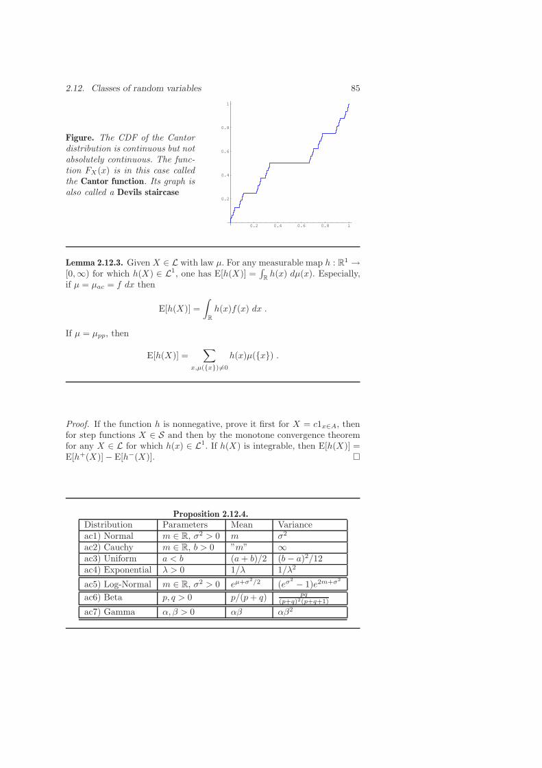
2.12. Classes of random variables 85
Figure. The CDF of the Cantordistribution is continuous but notabsolutely continuous. The func-tion FX(x) is in this case calledthe Cantor function. Its graph isalso called a Devils staircase
0.2 0.4 0.6 0.8 1
0.2
0.4
0.6
0.8
1
Lemma 2.12.3. Given X ∈ L with law µ. For any measurable map h : R1 →[0,∞) for which h(X) ∈ L1, one has E[h(X)] =
∫
Rh(x) dµ(x). Especially,
if µ = µac = f dx then
E[h(X)] =
∫
R
h(x)f(x) dx .
If µ = µpp, then
E[h(X)] =∑
x,µ(x) 6=0
h(x)µ(x) .
Proof. If the function h is nonnegative, prove it first for X = c1x∈A, thenfor step functions X ∈ S and then by the monotone convergence theoremfor any X ∈ L for which h(x) ∈ L1. If h(X) is integrable, then E[h(X)] =E[h+(X)] − E[h−(X)].
Proposition 2.12.4.Distribution Parameters Mean Varianceac1) Normal m ∈ R, σ2 > 0 m σ2
ac2) Cauchy m ∈ R, b > 0 ”m” ∞ac3) Uniform a < b (a+ b)/2 (b − a)2/12ac4) Exponential λ > 0 1/λ 1/λ2
ac5) Log-Normal m ∈ R, σ2 > 0 eµ+σ2/2 (eσ2 − 1)e2m+σ2
ac6) Beta p, q > 0 p/(p+ q) pq(p+q)2(p+q+1)
ac7) Gamma α, β > 0 αβ αβ2

86 Chapter 2. Limit theorems
Proposition 2.12.5.pp1) Bernoulli n ∈ N, p ∈ [0, 1] np np(1 − p)pp2) Poisson λ > 0 λ λpp3) Uniform n ∈ N (1 + n)/2 (n2 − 1)/12pp4) Geometric p ∈ (0, 1) (1 − p)/p (1 − p)/p2
pp5) First Success p ∈ (0, 1) 1/p (1 − p)/p2
sc1) Cantor - 1/2 1/8
Proof. These are direct computations, which we do in some of the examples:Exponential distribution:
E[Xp] =
∫ ∞
0
xpλe−λx dx =p
λE[Xp−1] =
p!
αp.
Poisson distribution:
E[X ] =
∞∑
k=0
ke−λλk
k!= λe−λ
∞∑
k=1
λk−1
(k − 1)!= λ .
For calculating higher moments, one can also use the probability generatingfunction
E[zX ] =∞∑
k=0
e−λ(λz)k
k!= e−λ(1−z)
and then differentiate this identity with respect to z at the place z = 0. Weget then
E[X ] = λ,E[X(X − 1)] = λ2,E[X3] = E[X(X − 1)(X − 2)], . . .
so that E[X2] = λ+ λ2 and Var[X ] = λ.Geometric distribution. Differentiating the identity for the geometric series
∞∑
k=0
xk =1
1 − x
gives∞∑
k=0
kxk−1 =1
(1 − x)2.
Therefore
E[Xp] =
∞∑
k=0
k(1 − p)kp =
∞∑
k=0
k(1 − p)kp = p
∞∑
k=1
k(1 − p)k =p
p2=
1
p.
For calculating the higher moments one can proceed as in the Poisson caseor use the moment generating function.Cantor distribution: because one can realize a random variable with the

2.12. Classes of random variables 87
Cantor distribution as X =∑∞n=1Xn/3
n, where the IID random variablesXn take the values 0 and 2 with probability p = 1/2 each, we have
E[X ] =
∞∑
n=1
E[Xn]
3n=
∞∑
n=1
1
3n=
1
1 − 1/3− 1 =
1
2
and
Var[X ] =
∞∑
n=1
Var[Xn]
3n=
∞∑
n=1
Var[Xn]
9n=
∞∑
n=1
1
9n=
1
1 − 1/9−1 =
9
8−1 =
1
8.
See also corollary (3.1.6) for an other computation.
Computations can sometimes be done in an elegant way using character-istic functions φX(t) = E[eitX ] or moment generating functions MX(t) =E[etX ]. With the moment generating function one can get the momentswith the moment formula
E[Xn] =
∫
R
xn dµ =dnMX
dtn(t)|t=0 .
For the characteristic function one obtains
E[Xn] =
∫
R
xn dµ = (−i)n dnφXdtn
(t)|t=0 .
Example. The random variable X(x) = x has the uniform distribution
on [0, 1]. Its moment generating function is MX(t) =∫ 1
0etx dx = (et −
1)/t = 1+t/2!+t2/3!+ . . . . A comparison of coefficients gives the momentsE[Xm] = 1/(m+ 1), which agrees with the moment formula.
Example. A random variableX which has the Normal distributionN(m,σ)
has the moment generating function MX(t) = etm+σ2t2/2. All the momentscan be obtained with the moment formula. For example, E[X ] = M ′
X(0) =m, E[X2] = M ′′
X(0) = m2 + σ2.
Example. For a Poisson distributed random variable X on Ω = N =
0, 1, 2, 3, . . . with P[X = k] = e−λ λk
k! , the moment generating function is
MX(t) =
∞∑
k=0
P[X = k]etk = eλ(1−et) .
Example. A random variable X on Ω = N = 0, 1, 2, 3, . . . with thegeometric distribution P[X = k] = p(1 − p)k has the moment generatingfunction
MX(t) =
∞∑
k=0
ektp(1 − p)k = p
∞∑
k=0
((1 − p)et)k =p
1 − (1 − p)et.

88 Chapter 2. Limit theorems
A random variable X on Ω = 1, 2, 3, . . . with the distribution of firstsuccess P[X = k] = p(1 − p)k−1, has the moment generating function
MX(t) =
∞∑
k=1
ektp(1 − p)k−1 = etp
∞∑
k=0
((1 − p)et)k =pet
1 − (1 − p)et.
Exercice. Compute the mean and variance of the Erlang distribution
f(x) =λktk−1
(k − 1)!e−λx
on the positive real line Ω = [0,∞) with the help of the moment generatingfunction. If k is allowed to be an arbitrary positive real number, then theErlang distribution is called the Gamma distribution.
Lemma 2.12.6. If X,Y are independent random variables, then their mo-ment generating functions satisfy
MX+Y (t) = MX(t) ·MY (t) .
Proof. If X and Y are independent, then also etX and etY are independent.Therefore,
E[et(X+Y )] = E[etXetY ] = E[etX ]E[etY ] = MX(t) ·MY (t) .
Example. The lemma can be used to compute the moment generatingfunction of the binomial distribution. A random variable X with bino-mial distribution can be written as a sum of IID random variables Xi
taking values 0 and 1 with probability 1 − p and p. Because for n = 1,we have MXi(t) = (1 − p) + pet, the moment generating function of Xis MX(t) = [(1 − p) + pet]n. The moment formula allows us to computemoments E[Xn] and central moments E[(X − E[X ])n] of X . Examples:
E[X ] = np
E[X2] = np(1 − p+ np)
Var[X ] = E[(X − E[X ])2] = E[X2] − E[X ]2 = np(1 − p)
E[X3] = np(1 + 3(n− 1)p+ (2 − 3n+ n2)p2)
E[X4] = np(1 + 7(n− 1)p+ 6(2 − 3n
+n2)p2 + (−6 + 11n− 6n2 + n3)p3)
E[(X − E[X ])4] = E[X4] − 8E[X ]E[X3] + 6E[X2]2 + E[X ]4
= np(1 − p)(1 + (5n− 6)p− (−6 + n+ 6n2)p2)

2.12. Classes of random variables 89
Example. The sum X+Y of a Poisson distributed random variable X withparameter λ and a Poisson distributed random variable Y with parameterµ is Poisson distributed with parameter λ+µ as can be seen by multiplyingtheir moment generating functions.
Definition. An interesting quantity for a random variable with a continuousdistribution with probability density fX is the Shannon entropy or simplyentropy
H(X) = −∫
R
f(x) log(f(x)) dx .
Without restricting the class of functions, H(X) is allowed to be −∞ or∞. The entropy allows to distinguish several distributions from others byasking for the distribution with the largest entropy. For example, among alldistribution functions on the positive real line [0,∞) with fixed expectationm = 1/λ, the exponential distribution λe−λ is the one with maximal en-tropy. We will return to these interesting entropy extremization questionslater.
Example. Let us compute the entropy of the random variable X(x) = xm
on ([0, 1],B, dx). We have seen earlier that the density of X is fX(x) =x1/m−1/m so that
H(X) = −∫ 1
0
(x1/m−1/m) log(x1/m−1/m) dx .
To compute this integral, note first that f(x) = xa log(xa) = axa log(x) has
the antiderivative ax1+a((1+a) log(x)−1)/(1+a)2 so that∫ 1
0 xa log(xa) dx =
−a/(1+a2) and H(X) = (1−m+log(m)). Because ddmH(Xm) = (1/m)−1
and d2
dm2H(Xm) = −1/m2, the entropy has its maximum at m = 1, wherethe density is uniform. The entropy decreases for m→ ∞. Among all ran-dom variables X(x) = xm, the random variable X(x) = x has maximalentropy.
Figure. The entropy of the ran-dom variables X(x) = xm on[0, 1] as a function of m. Themaximum is attained for m = 1,which is the uniform distribution
1 2 3 4 5
-4
-3
-2
-1

90 Chapter 2. Limit theorems
2.13 Weak convergence
Definition. Denote by Cb(R) the vector space of bounded continuous func-tions on R. This means that ||f ||∞ =
∑
x∈R |f(x)| <∞ for every f ∈ Cb(R).A sequence of Borel probability measures µn on R converges weakly to aprobability measure µ on R if for every f ∈ Cb(R) one has
∫
R
f dµn →∫
X
f dµ
in the limit n→ ∞.
Remark. For weak convergence, it is enough to test∫
Rf dµn →
∫
X f dµfor a dense set in Cb(R). This dense set can consist of the space P (R) ofpolynomials or the space C∞
b (R) of bounded, smooth functions.An important fact is that a sequence of random variables Xn convergesin distribution to X if and only if E[h(Xn)] → E[h(X)] for all smoothfunctions h on the real line. This will be used the proof of the central limittheorem.
Weak convergence defines a topology on the set M1(R) of all Borel proba-bility measures on R. Similarly, one has a topology for M1([a, b]).
Lemma 2.13.1. The set M1(I) of all probability measures on an intervalI = [a, b] is a compact topological space.
Proof. We need to show that any sequence µn of probability measures onI has an accumulation point. The set of functions fk(x) = xk on [a, b] spanall polynomials and so a dense set in Cb([a, b]). The sequence µn converges
to µ if and only if all the moments∫ b
a xk dµn converge for n→ ∞ and for
all k ∈ N. In other words, the compactness of M1([a, b]) is equivalent to thecompactness of the product space IN with the product topology, which isTychonovs theorem.
Remark. In functional analysis, a more general theorem called Banach-Alaoglu theorem is known: a closed and bounded set in the dual space X∗
of a Banach spaceX is compact with respect to the weak-* topology, wherethe functionals µn converge to µ if and only if µn(f) converges to µ(f) forall f ∈ X . In the present case, X = Cb[a, b] and the dual space X∗ is thespace of all signed measures on [a, b] (see [7]).
Remark. The compactness of probability measures can also be seen bylooking at the distribution functions Fµ(s) = µ((−∞, s]). Given a sequenceFn of monotonically increasing functions, there is a subsequence Fnk
whichconverges to an other monotonically increasing function F , which is again

2.13. Weak convergence 91
a distribution function. This fact generalizes to distribution functions onthe line where the limiting function F is still a right-continuous and non-decreasing function Helly’s selection theorem but the function F does notneed to be a distribution function any more, if the interval [a, b] is replacedby the real line R.
Definition. A sequence of random variables Xn converges weakly or in lawto a random variable X , if the laws µXn of Xn converge weakly to the lawµX of X .
Definition. Given a distribution function F , we denote by Cont(F ) the setof continuity points of F .
Remark. Because F is nondecreasing and takes values in [0, 1], the onlypossible discontinuity is a jump discontinuity. They happen at points ti,where ai = µ(ti) > 0. There can be only countably many such disconti-nuities, because for every rational number p/q > 0, there are only finitelymany ai with ai > p/q because
∑
i ai ≤ 1.
Definition. We say that a sequence of random variables Xn converges indistribution to a random variable X , if FXn(x) → FX(x) point wise for allx ∈ Cont(F ).
Theorem 2.13.2 (Weak convergence = convergence in distribution). A se-quence Xn of random variables converges in law to a random variable X ifand only if Xn converges in distribution to X .
Proof. (i) Assume we have convergence in law. We want to show that wehave convergence in distribution. Given s ∈ Cont(f) and δ > 0. Define acontinuous function 1(−∞,s] ≤ f ≤ 1(−∞,s+δ]. Then
Fn(s) =
∫
R
1(−∞,s] dµn ≤∫
R
f dµn ≤∫
R
1(−∞,s+δ] dµn = Fn(s+ δ) .
This gives
lim supn→∞
Fn(s) ≤ limn→∞
∫
f dµn =
∫
f dµ ≤ F (x+ δ) .
Similarly, we obtain with a function 1(−∞,s−δ] ≤ f ≤ 1(−∞,s]
lim infn→∞
Fn(s) ≥ limn→∞
∫
f dµn =
∫
f dµ ≥ F (s− δ) .
Since F is continuous at x we have for δ → 0:
F (s) = limδ→0
F (s− δ) ≤ lim infn→∞
Fn(s) ≤ lim supn→∞
Fn(s) ≤ F (s) .
92 Chapter 2. Limit theorems
That is we have established convergence in distribution.(ii) Assume now we have no convergence in law. There exists then a con-tinuous function f so that
∫
f dµn to∫
f dµ fails. That is, there is asubsequence and ǫ > 0 such that |
∫
f dµnk−
∫
f dµ| ≥ ǫ > 0. There existsa compact interval I such that |
∫
I f dµnk−
∫
I f dµ| ≥ ǫ/2 > 0 and wecan assume that µnk
and µ have support on I. The set of all probabilitymeasures on I is compact in the weak topology. Therefore, a subsequenceof dµnk
converges weakly to a measure ν and |ν(f) − µ(f)| ≥ ǫ/2. De-fine the π-system I of all intervals (−∞, s] | s continuity point of F .We have µn((−∞, s]) = FXn(s) → FX(s) = µ(−∞, s]). Using (i) we seeµnk
((−∞, s]) → ν(−∞, s] also, so that µ and ν agree on the π system I. Ifµ and ν agree on I, they agree on the π-system of all intervals (−∞, s].By lemma (2.1.4), we know that µ = ν on the Borel σ-algebra and so µ = ν.This contradicts |ν(f) − µ(f)| ≥ ǫ/2. So, the initial assumption of havingno convergence in law was wrong.
2.14 The central limit theorem
Definition. For any random variable X with non-zero variance, we denoteby
X∗ =(X − E[X ])
σ(X)
the normalized random variable, which has mean E[X∗] = 0 and varianceσ(X∗) =
√
Var[X∗] = 1. Given a sequence of random variables Xk, weagain use the notation Sn =
∑nk=1Xk.
Theorem 2.14.1 (Central limit theorem for independent L3 random vari-ables). Assume Xi ∈ L3 are independent and satisfy
M = supi
||Xi||3 <∞, δ = lim infn→∞
1
n
n∑
i=1
Var[Xi] > 0 .
Then S∗n converges in distribution to a random variable with standard
normal distribution N(0, 1):
limn→∞
P[S∗n ≤ x] =
1√2π
∫ x
−∞e−y
2/2 dy, ∀x ∈ R .

2.14. The central limit theorem 93
Figure. The probabil-ity density functionfS∗
1of the random
variable X(x) = x on[−1, 1].
Figure. The probabil-ity density functionfS∗
2of the random
variable X(x) = x on[−1, 1].
Figure. The probabil-ity density functionFS∗
3of the random
variable X(x) = x on[−1, 1].
Lemma 2.14.2. A N(0, σ2) distributed random variable X satisfies
E[|X |p] =1√π
2p/2σpΓ(1
2(p+ 1)) .
Especially E[|X |3] =√
8πσ
3.
Proof. With the density function f(x) = (2πσ2)−1/2e−x2
2σ2 , we have E[|X |p] =2
∫ ∞0xpf(x) dx which is after a substitution z = x2/(2σ2) equal to
1√π
2p/2σp∫ ∞
0
x12 (p+1)−1e−x dx .
The integral to the right is by definition equal to Γ(12 (p+ 1)).
After this preliminary computation, we turn to the proof of the centrallimit theorem.
Proof. Define for fixed n ≥ 1 the random variables
Yi =(Xi − E[Xi])
σ(Sn), 1 ≤ i ≤ n
so that S∗n =
∑ni=1 Yi. Define N(0, σ)-distributed random variables Yi hav-
ing the property that the set of random variables
Y1, . . . , Yn, Y1, . . . Yn
are independent. The distribution of Sn =∑ni=1 Yi is just the normal distri-
bution N(0, 1). In order to show the theorem, we have to prove E[f(S∗n)]−

94 Chapter 2. Limit theorems
E[f(Sn)] → 0 for any f ∈ Cb(R). It is enough to verify it for smooth f .Define
Zk = Y1 + . . . Yk−1 + Yk+1 + · · · + Yn .
Note that Z1 + Y1 = S∗n and Zn + Yn = Sn. Using first a telescopic sum
and then Taylor’s theorem, we can write
f(S∗n) − f(Sn) =
n∑
k=1
[f(Zk + Yk) − f(Zk + Yk)]
=
n∑
k=1
[f ′(Zk)(Yk − Yk)] +
n∑
k=1
[1
2f ′′(Zk)(Y
2k − Y 2
k )]
+
n∑
k=1
[R(Zk, Yk) +R(Zk, Yk)]
with a Taylor rest term R(Z, Y ), which can depend on f . We get therefore
|E[f(S∗n)] − E[f(Sn)]| ≤
n∑
k=1
E[|R(Zk, Yk)|] + E[|R(Zk, Yk)|] . (2.7)
Because Yk are N(0, σ2)-distributed, we get by lemma (2.14.2) and theJensen inequality (2.5.1)
E[|Yk|3] =
√
8
πσ3 =
√
8
πE[|Yk|2]3/2 ≤
√
8
πE[|Yk|3] .
Taylor’s theorem gives |R(Zk, Yk)| ≤ const · |Yk|3 so that
n∑
k=1
E[|R(Zk, Yk)|] + E[|R(Zk, Yk)|] ≤ const ·n
∑
k=1
E[|Yk|3]
≤ const · n · supi
||Xi||3/Var[Sn]3/2
= const · supi ||Xi||3(Var[Sn]/n)3/2
· 1√n
=M
δ3/21√n
=C(f)√n
→ 0 .
We have seen that for every smooth f ∈ Cb(R) there exists a constant C(f)such that |E[f(S∗
n)] − E[f(Sn)]| ≤ C(f)/√n.
if we assume the Xi to be identically distributed, we can relax the conditionXi ∈ L3 to Xi ∈ L2:
Theorem 2.14.3 (Central limit theorem for IID L2 random variables). IfXi ∈ L2 are IID and satisfy 0 < Var[Xi], then S∗
n converges weakly to arandom variable with standard normal distribution N(0, 1).

2.14. The central limit theorem 95
Proof. The same proof gives equation (5.4). We change the estimation ofTaylor |R(z, y)| ≤ δ(y) · y2 with δ(y) → 0 for |y| → 0. Using the IIDproperty and using dominated convergence we can estimate the rest term
R =
n∑
k=1
E[|R(Zk, Yk)|] + E[|R(Zk, Yk)|]
as follows:
R ≤n
∑
k=1
E[δ(Yk)Y2k ] + E[δ(Yk)Y
2k ]
= n · E[δ(X1
σ√n
)X2
1
σ2n] + n · E[δ(
X1
σ√n
)X2
1
σ2n]
≤ n · E[δ(X1
σ√n
)]E[X2
1
σ2n] + n · E[δ(
X1
σ√n
)]E[X2
1
σ2n]
= E[δ(X1
σ√n
)]E[X2
1
σ2] + E[δ(
X1
σ√n
)]E[X2
1
σ2]
≤ E[δ(X1
σ√n
)]C → 0
The central limit theorem can be interpreted as a solution to a fixed pointproblem:
Definition. Let P0,1 be the space of probability measure µ on (R,BR) whichhave the properties that
∫
Rx2 dµ(x) = 1,
∫
Rx dµ(x) = 0. Define the map
Tµ(A) =
∫
R
∫
R
1A(x+ y√
2)µ(dx) µ(dy)
on P0,1.
Corollary 2.14.4. The only attracting fixed point of T on P0,1 is the law ofthe standard normal distribution.
Proof. If µ is the law of a random variable X with Var[X ] = 1 and E[X ] =0. Then T (µ) is the law of the normalized random variable (X+X)/
√2 be-
cause the independent random variables X,Y can be realized on the proba-bility space (R2,B, µ×µ) as coordinate functions X((x, y)) = x, Y ((x, y)) =y. Then T (µ) is obviously the law of (X + Y )/
√2. Now use that T n(X) =
(S2n)∗ converges in distribution to N(0, 1).

96 Chapter 2. Limit theorems
For independent 0 − 1 experiments with win probability p ∈ (0, 1), thecentral limit theorem is quite old. In this case
limn→∞
P[(Sn − np)
√
np(1 − p)≤ x] =
1
2π
∫ x
−∞e−y
2/2 dy
as had been shown by de Moivre in 1730 in the case p = 1/2 and for generalp ∈ (0, 1) by Laplace in 1812. It is a direct consequence of the central limittheorem:
Corollary 2.14.5. (DeMoivre-Laplace limit theorem) The distribution ofX∗n
converges to the normal distribution if Xn has the binomial distributionB(n, p).
For more general versions of the central limit theorem, see [105]. The nextlimit theorem for discrete random variables illustrates, why Poisson dis-tribution on N is natural. Denote by B(n, p) the binomial distribution on1, . . . , n and with Pα the Poisson distribution on N \ 0 .
Theorem 2.14.6 (Poisson limit theorem). Let Xn be a B(n, pn)-distributedand suppose npn → α. Then Xn converges in distribution to a randomvariable X with Poisson distribution with parameter α.
Proof. We have to show that P[Xn = k] → P[X = k] for each fixed k ∈ N.
P[Xn = k] =
(
nk
)
pkn(1 − pn)n−k
=n(n− 1)(n− 2) . . . (n− k + 1)
k!pkn(1 − pn)
n−k
∼ 1
k!(npn)
k(1 − npnn
)n−k → αk
k!e−α .

2.14. The central limit theorem 97
0.1
0.2
0.3
0.4
0.5
Figure. The binomialdistribution B(2, 1/2)has its support on0, 1, 2 .
0.1
0.2
0.3
0.4
Figure. The binomialdistribution B(5, 1/5)has its support on0, 1, 2, 3, 4, 5 .
0.05
0.10
0.15
0.20
0.25
0.30
0.35
Figure. The Pois-son distributionwith α = 1 onN = 0, 1, 2, 3, . . . .
Exercice. It is custom to use the notation
Φ(s) = FX(s) =1√2π
∫ s
−∞e−y
2/2 dy
for the distribution function of a random variableX which has the standardnormal distribution N(0, 1). Given a sequence of IID random variables Xn
with this distribution.a) Justify that one can estimate for large n probabilities
P[a ≤ S∗n ≤ b] ∼ Φ(b) − Φ(a) .
b) Assume Xi are all uniformly distributed random variables in [0, 1].Estimate for large n
P[|Sn/n− 0.5| ≥ ǫ]
in terms of Φ, ǫ and n.c) Compare the result in b) with the estimate obtained in the weak law oflarge numbers.
Exercice. Define for λ > 0 the transformation
Tλ(µ)(A) =
∫
R
∫
R
1A(x+ y
λ) dµ(x) dµ(y)
in P = M1(R), the set of all Borel probability measures on R. For which λcan you describe the limit?
98 Chapter 2. Limit theorems
2.15 Entropy of distributions
Denote by ν a (not necessarily finite) measure on a measure space (Ω,A).An example is the Lebesgue measure on R or the counting measure on N.Note that the measure is defined only on a δ-subring of A since we did notassume that ν is finite.
Definition. A probability measure µ on R is called ν absolutely continuous,if there exists a density f ∈ L1(ν) such that µ = fν. If µ is ν-absolutelycontinuous, one writes µ≪ ν. Call P(ν) the set of all ν absolutely contin-uous measures. The set P(ν) is the set of functions f ∈ L1(ν) satisfyingf ≥ 0 and
∫
f(x) dν(x) = 1.
Remark. The fact that µ≪ ν defined earlier is equivalent to this is calledthe Radon-Nykodym theorem ([?]). The function f is therefore called theRadon-Nykodym derivative of µ with respect to ν.
Example. If ν is the counting measure N = 0, 1, 2, . . . and ν is thelaw of the geometric distribution with parameter p, then the density isf(k) = p(1 − p)k.
Example. If ν is the Lebesgue measure on (−∞,∞) and µ is the law of
the standard normal distribution, then the density is f(x) = e−x2/2/
√2π.
There is a multi-variable calculus trick using polar coordinates, which im-mediately shows that f is a density:
∫ ∫
R2
e−(x2+y2)/2 dxdy =
∫ ∞
0
∫ 2π
0
e−r2/2 rdθdr = 2π .
Definition. For any probability measure µ ∈ P(ν) define the entropy
H(µ) =
∫
Ω
−f(ω) log(f(ω)) dν(ω) .
It generalizes the earlier defined Shannon entropy, where the assumptionhad been dν = dx.
Example. Let ν be the counting measure on a countable set Ω, where Ais the σ-algebra of all subsets of Ω and let the measure ν is defined on theδ-ring of all finite subsets of Ω. In this case,
H(µ) =∑
ω∈Ω
−f(ω) log(f(ω)) .
For example, for Ω = N = 0, 1, 2, 3, . . . with counting measure ν, thegeometric distribution P[k] = p(1 − p)k has the entropy
∞∑
k=0
−(1 − p)kp log((1 − p)kp) = log(1 − p
p) − log(1 − p)
p.

2.15. Entropy of distributions 99
Example. Let ν be the Lebesgue measure on R. If µ = fdx has a densityfunction f , we have
H(µ) =
∫
R
−f(x) log(f(x)) dx .
For example, for the standard normal distribution µ with probability den-sity function f(x) = 1√
2πe−x
2/2, the entropy is H(f) = (1 + log(2π))/2.
Example. If ν is the Lebesgue measure dx on Ω = R+ = [0,∞). A randomvariable on Ω with probability density function f(x) = λe−λx is called theexponential distribution. It has the mean 1/λ. The entropy of this distri-bution is (log(λ) − 1)/λ.
Example. If ν is a probability measure on R, f a density and
A = A1, . . . , .An
is a partition on R. For the step function
f =
n∑
i=1
(
∫
Ai
f dν)1Ai ∈ S(ν) ,
the entropy H(f ν) is equal to
H(Ai) =∑
i
−ν(Ai) log(ν(Ai))
which is called the entropy of the partition Ai. The approximation of thedensity f by a step functions f is called coarse graining and the entropyof f is called the coarse grained entropy. It has first been considered byGibbs in 1902.
Remark. In ergodic theory, where one studies measure preserving trans-formations T of probability spaces, one is interested in the growth rate ofthe entropy of a partition generated by A, T (A), .., T n(A). This leads tothe notion of an entropy of a measure preserving transformation calledKolmogorov-Sinai entropy.
Interpretation. Assume that Ω is finite and that ν the counting measureand µ(ω) = f(ω) the probability distribution of random variable de-scribing the measurement of an experiment. If the event ω happens, then− log(f(ω)) is a measure for the information or ”surprise” that the eventhappens. The averaged information or surprise is
H(µ) =∑
ω
−f(ω) log(f(ω)) .

100 Chapter 2. Limit theorems
If f takes only the values 0 or 1, which means that µ is deterministic,then H(µ) = 0. There is no surprise and what the measurements show, isthe reality. On the other hand, if f is the uniform distribution on Ω, thenH(µ) = log(|Ω|). We will see in a moment that this is the maximal entropy.
Definition. Given two probability measures µ = fν and µ = f ν which areboth absolutely continuous with respect to ν. Define the relative entropy
H(µ|µ) =
∫
f(ω) log(f(ω)
f(ω)) dν(x) ∈ [0,∞] .
It is the expectation Eµ[l] of the Likelihood coefficient l = log( f(x)f(x) ). The
negative relative entropy −H(µ|µ) is also called the conditional entropy.One writes also H(f |f) instead of H(µ|µ).
Theorem 2.15.1 (Gibbs inequality). 0 ≤ H(µ|µ) ≤ +∞ and H(µ|µ) = 0 ifand only if µ = µ.
Proof. We can assumeH(µ|µ) <∞. The function u(x) = x log(x) is convexon R+ = [0,∞) and satisfies u(x) ≥ x− 1.
H(µ|µ) =
∫
Ω
f(ω)u(f(x)
f(x)) dν ≥
∫
Ω
f(ω)(f(x)
f(x)− 1) dν = 0 .
If µ = µ, then f = f almost everywhere and H(µ|µ) = 0.On the other hand, if H(µ|µ) = 0, then by the Jensen inequality (2.5.1)
0 = Eµ[u(f
f)] ≥ u(Eµ[
f
f]) = u(1) = 0 .
Therefore, Eµ[u(ff )] = u(Eµ[
ff ]). The strict convexity of u implies that f
f
must be a constant. Since both f and f are densities, we have f = f .
Remark. The relative entropy can be used to measure the distance betweentwo distributions. It is not a metric although. The relative entropy is alsoknown under the name Kullback-Leibler divergence or Kullback-Leiblermetric, if ν = dx [85].

2.15. Entropy of distributions 101
Theorem 2.15.2 (Distributions with maximal entropy). The following dis-tributions have maximal entropy.a) If Ω is finite with counting measure ν. The uniform distribution on Ωhas maximal entropy among all distributions on Ω. It is unique with thisproperty.b) Ω = N with counting measure ν. The geometric distribution withparameter p = c−1 has maximal entropy among all distributions onN = 0, 1, 2, 3, . . . with fixed mean c. It is unique with this property.c) Ω = 0, 1N with counting measure ν. The product distribution ηN ,where η(1) = p, η(0) = 1− p with p = c/N has maximal entropy among all
distributions satisfying E[SN ] = c, where SN (ω) =∑N
i=1 ωi. It is uniquewith this property.d) Ω = [0,∞) with Lebesgue measure ν. The exponential distribution withdensity f(x) = λe−λx with parameter λ on Ω has the maximal entropyamong all distributions with fixed mean c = 1/λ. It is unique with thisproperty.e) Ω = R with Lebesgue measure ν. The normal distribution N(m,σ2)has maximal entropy among all distributions with fixed mean m and fixedvariance σ2. It is unique with this property.f) Finite measures. Let (Ω,A) be an arbitrary measure space for which0 < ν(Ω) <∞. Then the measure ν with uniform distribution f = 1/ν(Ω)has maximal entropy among all other measures on Ω. It is unique with thisproperty.
Proof. Let µ = fν be the measure of the distribution from which we wantto prove maximal entropy and let µ = fν be any other measure. The aimis to show H(µ|µ) = H(µ) −H(µ) which implies the maximality since bythe Gibbs inequality lemma (2.15.1) H(µ|µ) ≥ 0.In general,
H(µ|µ) = −H(µ) −∫
Ω
f(ω) log(f(ω)) dν
so that in each case, we have to show
H(µ) = −∫
Ω
f(ω) log(f(ω)) dν . (2.8)
With
H(µ|µ) = H(µ) −H(µ)
we also have uniqueness: if two measures µ, µ have maximal entropy, thenH(µ|µ) = 0 so that by the Gibbs inequality lemma (2.15.1) µ = µ.
a) The density f = 1/|Ω| is constant. Therefore H(µ) = log(|Ω|) and equa-tion (2.8) holds.

102 Chapter 2. Limit theorems
b) The geometric distribution on N = 0, 1, 2, . . . satisfies P[k] = f(k) =p(1 − p)k, so that
∫
Ω
f(ω) log(f(ω)) dν = log(p) +
∫
f(ω)k log(1 − p) dν
= log(p) − log(1 − p)
∫
Ω
f(ω) dν(ω)
= log(p
(1 − p))
which is also the entropy of µ.
c) The discrete density is f(ω) = pSN (1 − p)N−SN so that
log(f(k)) = SN log(p) + (N − SN ) log(1 − p)
and∑
k
f(k) log(f(k)) = E[SN ] log(p) + (N − E[SN ]) log(1 − p) .
The claim follows since we fixed E[SN ].
d) The density is f(x) = αe−αx, so that log(f(x)) = log(α) − αx. Theclaim follows since we fixed E[X ] =
∫
x dµ(x) was assumed to be fixed forall distributions.
e) For the normal distribution log(f(x)) = a + b(x − m)2 with two realnumber a, b depending only on m and σ. The claim follows since we fixedVar[X ] = E[(x−m)2] for all distributions.
f) The density f = 1 is constant. Therefore H(µ) = 0 which is also on theright hand side of equation (2.8).
Remark. This result has relations to the foundations of thermodynamics,where one considers the phase space of N particles moving in a finite regionin Euclidean space. The energy surface is then a compact surface Ω and themotion on this surface leaves a measure ν invariant which is induced fromthe flow invariant Lebesgue measure. The measure ν is called the micro-canonical ensemble. According to f) in the above, it is the measure whichmaximizes entropy.
Remark. Let us try to get the maximal distribution using calculus of vari-ations. In order to find the maximum of the functional
H(f) = −∫
f log(f) dν
on L1(ν) under the constraints
F (f) =
∫
Ω
f dν = 1, G(f) =
∫
Ω
Xf dν = c ,

2.15. Entropy of distributions 103
we have to find the critical points of H = H − λF − µG In infinite dimen-sions, constrained critical points are points, where the Lagrange equations
∂
∂fH(f) = λ
∂
∂fF (f) + µ
∂
∂fG(f)
F (f) = 1
G(f) = c
are satisfied. The derivative ∂/∂f is the functional derivative and λ, µ arethe Lagrange multipliers. We find (f, λ, ν) as a solution of the system ofequations
−1 − log(f(x)) = λ+ µx,∫
Ω
f(x) dν(x) = 1,
∫
Ω
xf(x) dν(x) = c
by solving the first equation for f :
f = e−λ−µx+1
∫
e−λ−µx+1 dν(x) = 1
∫
xe−λ−µx+1 dν(x) = c
dividing the third equation by the second, so that we can get µ from theequation
∫
xe−µxx dν(x) = c∫
e−µ(x) dν(x) and λ from the third equatione1+λ =
∫
e−µx dν(x). This variational approach produces critical points ofthe entropy. Because the Hessian D2(H) = −1/f is negative definite, it isalso negative definite when restricted to the surface in L1 determined bythe restrictions F = 1, G = c. This indicates that we have found a globalmaximum.
Example. For Ω = R, X(x) = x2, we get the normal distribution N(0, 1).
Example. For Ω = N, X(n) = ǫn, we get f(n) = e−ǫnλ1/Z(f) with Z(f) =∑
n e−ǫnλ1 and where λ1 is determined by
∑
n ǫne−ǫnλ1 = c. This is called
the discrete Maxwell-Boltzmann distribution. In physics, one writes λ−1 =kT with the Boltzmann constant k, determining T , the temperature.
Here is a dictionary matching some notions in probability theory with cor-responding terms in statistical physics. The statistical physics jargon isoften more intuitive.
Probability theory Statistical mechanics
Set Ω Phase spaceMeasure space Thermodynamic systemRandom variable Observable (for example energy)Probability density Thermodynamic stateEntropy Boltzmann-Gibbs entropyDensities of maximal entropy Thermodynamic equilibriaCentral limit theorem Maximal entropy principle

104 Chapter 2. Limit theorems
Distributions, which maximize the entropy possibly under some constraintare mathematically natural because they are critical points of a variationalprinciple. Physically, they are natural, because nature prefers them. Fromthe statistical mechanical point of view, the extremal properties of entropyoffer insight into thermodynamics, where large systems are modeled withstatistical methods. Thermodyanamic equilibria often extremize variationalproblems in a given set of measures.
Definition. Given a measure space (Ω,A) with a not necessarily finitemeasure ν and a random variable X ∈ L. Given f ∈ L1 leading to theprobability measure µ = fν. Consider the moment generating functionZ(λ) = Eµ[e
λX ] and define the interval Λ = λ ∈ R | Z(λ) < ∞ in R.For every λ ∈ Λ we can define a new probability measure
µλ = fλν =eλX
Z(λ)µ
on Ω. The set
µλ | λ ∈ Λ
of measures on (Ω,A) is called the exponential family defined by ν and X .
Theorem 2.15.3 (Minimizing relative entropy). For all probability measuresµ which are absolutely continuous with respect to ν, we have for all λ ∈ Λ
H(µ|µ) − λEµ[X ] ≥ − logZ(λ) .
The minimum − logZ(λ) is obtained for µλ.
Proof. For every µ = f ν, we have
H(µ|µ) =
∫
Ω
f log(f
fλ) · fλ
fdν
= −H(µ|µλ) + (− log(Z(λ)) + λEµ[X ]) .
For µ = µλ, we have
H(µλ|µ) = − log(Z(λ)) + λEµλ[X ] .
Therefore
H(µ|µ) − λEµ[X ] = H(µ|µλ) − log(Z(λ)) ≥ − logZ(λ) .
The minimum is obtained for µ = µλ.

2.15. Entropy of distributions 105
Corollary 2.15.4. (Minimizers for relative entropy)a) µλ minimizes the relative entropy µ 7→ H(µ|µ) among all ν-absolutelycontinuous measures µ with fixed Eµ[X ].b) If we fix λ by requiring Eµλ
[X ] = c, then µλ maximizes the entropyH(µ) among all measures µ satisfying Eµ[X ] = c.
Proof. a) Minimizing µ 7→ H(µ|µ) under the constraint Eµ[X ] = c is equiv-alent to minimize
H(µ|µ) − λEµ[X ],
and to determine the Lagrange multiplier λ by Eµλ[X ] = c. The above
theorem shows that µλ is minimizing that.b) If µ = fν, µλ = e−λXf/Z, then
0 ≤ H(µ, µλ) = −H(µ) + (− log(Z)) − λEµ[X ] = −H(µ) +H(µλ) .
Corollary 2.15.5. If ν = µ is a probability measure, then µλ maximizes
F (µ) = H(µ) + λEµ[X ]
among all measures µ which are absolutely continuous with respect to µ.
Proof. Take µ = ν. Since then f = 1, H(µ|µ) = −H(µ). The claim followsfrom the theorem since a minimum of H(µ|µ) − λEµ[X ] corresponds to amaximum of F (µ).
This corollary can also be proved by calculus of variations, namely byfinding the minimum of F (f) =
∫
f log(f) + Xf dν under the constraint∫
f dν = 1.
Remark. In statistical mechanics, the measure µλ is called the Gibbs distri-bution or Gibbs canonical ensemble for the observableX and Z(λ) is calledthe partition function. In physics, one uses the notation λ = −(kT )−1,where T is the temperature. Maximizing H(µ)− (kT )−1Eµ[X ] is the sameas minimizing Eµ[X ] − kTH(µ) which is called the free energy if X isthe Hamiltonian and Eµ[X ] is the energy. The measure µ is the a priorimodel, the micro canonical ensemble. Adding the restriction that X hasa specific expectation value c = Eµ[X ] leads to the probability measureµλ, the canonical ensemble. We illustrated two physical principles: naturemaximizes entropy when the energy is fixed and minimizes the free energy,when energy is not fixed.

106 Chapter 2. Limit theorems
Example. Take on the real line the Hamiltonian X(x) = x2 and a measureµ = fdx, we get the energy
∫
x2 dµ. Among all symmetric distributionsfixing the energy, the Gaussian distribution maximizes the entropy.
Example. Let Ω = N = 0, 1, 2, . . . and X(k) = k and let ν be thecounting measure on Ω and µ the Poisson measure with parameter 1. Thepartition function is
Z(λ) =∑
k
eλke−1
k!= exp(eλ − 1)
so that Λ = R and µλ is given by the weights
µλ(k) = exp(e−λ + 1)eλke−1
k!= e−α
αk
k!,
where α = eλ = 0. The exponential family of the Poisson measure is thefamily of all Poisson measures.
Example. The geometric distribution on N = 0, 1, 2, 3, . . . is an expo-nential family.
Example. The product measure on Ω = 0, 1 N with win probability p isan exponential family with respect to X(k) = k.
Example. Ω = 1, . . . , N, ν the counting measure and let µp be the bino-mial distribution with p. Take µ = µ1/2 and X(k) = k. Since
0 ≤ H(µ|µ) = H(µ|µp) + log(p)E[X ] + log(1 − p)E[(N − E[X ])]
= −H(µ|µp) +H(µp) ,
µp is an exponential family.
Remark. There is an obvious generalization of the maximum entropy prin-ciple to the case, when we have finitely many random variables Xini=1.Given µ = fν we define the (n-dimensional) exponential family
µλ = fλν =e
Pni=1 λiXi
Z(λ)µ ,
where
Z(λ) = Eµ[ePn
i=1 λiXi ]
is the partition function defined on a subset Λ of Rn.

2.16. Markov operators 107
Theorem 2.15.6. For all probability measures µ which are absolutely con-tinuous with respect to ν, we have for all λ ∈ Λ
H(µ|µ) −∑
i
λiEµ[Xi] ≥ − logZ(λ) .
The minimum − logZ(λ) is obtained for µλ. If we fix λi by requiringEµλ
[Xi] = ci, then µλ maximizes the entropy H(µ) among all measuresµ satisfying Eµ[Xi] = ci.Assume ν = µ is a probability measure. The measure µλ maximizes
F (µ) = H(µ) + λEµ[X ] .
Proof. Take the same proofs as before by replacing λX with λ · X =∑
i λiXi.
2.16 Markov operators
Definition. Given a not necessarily finite probability space (Ω,A, ν). Alinear operator P : L1(Ω) → L1(Ω) is called a Markov operator, if
f ≥ 0 ⇒ Pf ≥ 0,f ≥ 0 ⇒ ||Pf ||1 = ||f ||1.
Remark. In other words, a Markov operator P has to leave the closedpositive cone invariant L1
+ = f ∈ L1 | f ≥ 0 and preserve the norm onthat cone.
Remark. A Markov operator on (Ω,A, ν) leaves invariant the set D(ν) =f ∈ L1 | f ≥ 0, ||f ||1 = 1 of probability densities. They correspondbijectively to the set P(ν) of probability measures which are absolutelycontinuous with respect to ν. A Markov operator is therefore also called astochastic operator.
Example. Let T be a measure preserving transformation on (Ω,A, ν). It iscalled nonsingular if T ∗ν is absolutely continuous with respect to ν. Theunique operator P : L1 → L1 satisfying
∫
A
Pf dν =
∫
T−1A
f dν
is called the Perron-Frobenius operator associated to T . It is a Markovoperator. Closely related is the operator Pf(x) = f(Tx) for measure pre-serving invertible transformations. This Koopman operator is often studiedon L2, but it becomes a Markov operator when considered as a transfor-mation on L1.

108 Chapter 2. Limit theorems
Exercice. Assume Ω = [0, 1] with Lebesgue measure µ. Verify that thePerron-Frobenius operator for the tent map
T (x) =
2x , x ∈ [0, 1/2]2(1 − x) , x ∈ [1/2, 1]
is Pf(x) = 12 (f(1
2x) + f(1 − 12x)).
Here is an abstract version of the Jensen inequality (2.5.1). It is due to M.Kuczma. See [61].
Theorem 2.16.1 (Jensen inequality for positive operators). Given a convexfunction u and an operator P : L1 → L1 mapping positive functions intopositive functions satisfying P1 = 1, then
u(Pf) ≤ Pu(f)
for all f ∈ L1+ for which Pu(f) exists.
Proof. We have to show u(Pf)(ω) ≤ Pu(f)(ω) for almost all ω ∈ Ω. Givenx = (Pf)(ω), there exists by definition of convexity a linear function y 7→ay + b such that u(x) = ax+ b and u(y) ≥ ay + b for all y ∈ R. Therefore,since af + b ≤ u(f) and P is positive
u(Pf)(ω) = a(Pf)(ω) + b = P (af + b)(ω) ≤ P (u(f))(ω) .
The following theorem states that relative entropy does not increase alongorbits of Markov operators. The assumption that f > 0 is mapped intoitself is actually not necessary, but simplifies the proof.
Theorem 2.16.2 (Voigt, 1981). Given a Markov operator P which mapsf > 0 into itself. For all f, g ∈ L1
+,
H(Pf |Pg) ≤ H(f |g) .
Proof. We can assume that g(ω) = 0 ⊂ A = f(ω) = 0 because nothingis to show in the case H(f |g) = ∞. By restriction to the measure spacespace (Ac,A ∩ Ac, ν(· ∩ A)), we can assume f > 0, g > 0 so that by ourassumption also Pf > 0 and Pg > 0.

2.16. Markov operators 109
(i) Assume first (f/g)(ω) ≤ c for some constant c ∈ R.For fixed g, the linear operator Rh = P (hg)/P (g) maps positive functionsinto positive functions. Take the convex function u(x) = x log(x) and puth = f/g. Using Jensen’s inequality, we get
Pf
Pglog
Pf
Pg= u(Rh) ≤ Ru(h) =
P (f log(f/g))
Pg
which is equivalent to Pf log PfPg ≤ P (f log(f/g)). Integration gives
H(Pf |Pg) =
∫
Pf logPf
Pgdν
≤∫
P (f log(f/g)) dν =
∫
f log(f/g) dν = H(f |g) .
(ii) Define fk = inf(f, kg) so that fk/g ≤ k. We have fk ⊂ fk+1 andfk → f in L1. From (i) we know that H(Pfk|Pg) ≤ H(fk|g). We canassume H(f |g) < ∞ because the result is trivially true in the other case.Define B = f ≤ g. On B, we have fk log(fk/g) = f log(f/g) and on Ω\Bwe have
fk log(fk/g) ≤ fk+1 log(fk+1/g)u→ f log(f/g)
so that by Lebesgue dominated convergence theorem,
H(f |g) = limk→∞
H(fk|g) .
As an increasing sequence, Pfk converges to Pf almost everywhere. Theelementary inequality x log(x) − x ≥ x log(y) − y for all x ≥ y ≥ 0 gives
(Pfk) log(Pfk) − (Pfk) log(Pg) − (Pfk) + (Pg) ≥ 0 .
Integration gives with Fatou’s lemma (2.4.2)
H(Pf |Pg)− ||Pf || + ||Pg|| ≤ lim infk→∞
H(Pfk|Pg) − ||Pfk|| + ||Pg||
and so H(Pf |Pg) ≤ lim infk→∞H(Pfk|Pg).
Corollary 2.16.3. For an invertible Markov operator P, the relative entropyis constant: H(Pf |Pg) = H(f |g).
Proof. Because P and P−1 are both Markov operators,
H(f |g) = H(PP−1f |PP−1g) ≤ H(P−1f |P−1g) ≤ H(f |g) .

110 Chapter 2. Limit theorems
Example. If a measure preserving transformation T is invertible, then thecorresponding Koopman operator and Perron-Frobenius operators preserverelative entropy.
Corollary 2.16.4. The operator T (µ)(A) =∫
R2 1A(x+y√2
) dµ(x) dµ(y) does
not decrease entropy.
Proof. Denote by Xµ a random variable having the law µ and with µ(X)the law of a random variable. For a fixed random variable Y , we define theMarkov operator
PY (µ) = µ(Xµ + Y√
2) .
Because the entropy is nondecreasing for each PY , we have this propertyalso for the nonlinear map T (µ) = PXµ(µ).
We have shown as a corollary of the central limit theorem that T has aunique fixed point attracting all of P0,1. The entropy is also strictly in-creasing at infinitely many points of the orbit T n(µ) since it converges tothe fixed point with maximal entropy. It follows that T is not invertible.
More generally: given a sequence Xn of IID random variables. For every n,the map Pn which maps the law of S∗
n into the law of S∗n+1 is a Markov
operator which does not increase entropy. We can summarize: summing upIID random variables tends to increase the entropy of the distributions.A fixed point of a Markov operator is called a stationary state or in morephysical language a thermodynamic equilibrium. Important questions are:is there a thermodynamic equilibrium for a given Markov operator P andif yes, how many are there?
2.17 Characteristic functions
Distribution functions are in general not so easy to deal with, as for ex-ample, when summing up independent random variables. It is thereforeconvenient to deal with its Fourier transforms, the characteristic functions.It is an important topic by itself [60].
Definition. Given a random variable X , its characteristic function is a real-valued function on R defined as
φX(u) = E[eiuX ] .
If FX is the distribution function of X and µX its law, the characteristicfunction of X is the Fourier-Stieltjes transform
φX(t) =
∫
R
eitx dFX(x) =
∫
R
eitx µX(dx) .

2.17. Characteristic functions 111
Remark. If FX is a continuous distribution function dFX(x) = fX(x) dx,then φX is the Fourier transform of the density function fX :
∫
R
eitx fX(x) dx .
Remark. By definition, characteristic functions are Fourier transforms ofprobability measures: if µ is the law of X , then φX = µ.
Example. For a random variable with density fX(x) = xm/(m + 1) onΩ = [0, 1] the characteristic function is
φX(t) =
∫ 1
0
eitxxm dx/(m+ 1) =m!(1 − eitem(−it))(−it)1+m(m+ 1)
,
where en(x) =∑nk=0 x
k/(k!) is the n’th partial exponential function.
Theorem 2.17.1 (Levy formula). The characteristic function φX determinesthe distribution of X . If a, b are points of continuity of F , then
FX(b) − FX(a) =1
2π
∫ ∞
−∞
e−ita − e−itb
itφX(t) dt . (2.9)
In general, one has
1
2π
∫ ∞
−∞
e−ita − e−itb
itφX(t) dt = µ[(a, b)] +
1
2µ[a] + 1
2µ[b] .
Proof. Because a distribution function F has only countably many points ofdiscontinuities, it is enough to determine F (b)−F (a) in terms of φ if a andb are continuity points of F . The verification of the Levy formula is thena computation. For continuous distributions with density F ′
X = fX is theinverse formula for the Fourier transform: fX(a) = 1
2π
∫ ∞−∞ e−itaφX(t) dt
so that FX(a) = 12π
∫ ∞−∞
e−ita
−it φX(t) dt. This proves the inversion formulaif a and b are points of continuity.The general formula needs only to be verified when µ is a point measureat the boundary of the interval. By linearity, one can assume µ is locatedon a single point b with p = P[X = b] > 0. The Fourier transform of theDirac measure pδb is φX(t) = peitb. The claim reduces to
1
2π
∫ ∞
−∞
e−ita − e−itb
itpeitb dt =
p
2
which is equivalent to the claim limR→∞∫ R
−Reitc−1it dt = π for c > 0.
Because the imaginary part is zero for every R by symmetry, only
limR→∞
∫ R
−R
sin(tc)
tdt = π
112 Chapter 2. Limit theorems
remains. The verification of this integral is a prototype computation inresidue calculus.
Theorem 2.17.2 (Characterization of weak convergence). A sequence Xn
of random variables converges weakly to X if and only if its characteristicfunctions converge point wise:
φXn(x) → φX .
Proof. Because the exponential function eitx is continuous for each t, itfollows from the definition that weak convergence implies the point wiseconvergence of the characteristic functions. From formula (2.9) follows thatif the characteristic functions converge point wise, then convergence in dis-tribution takes place. We have learned in lemma (2.13.2) that weak con-vergence is equivalent to convergence in distribution.
Example. Here is a table of characteristic functions (CF) φX(t) = E[eitX ]and moment generating functions (MGF) MX(t) = E[etX ] for some familiarrandom variables:
Distribution Parameter CF MGF
Normal m ∈ R, σ2 > 0 emit−σ2t2/2 emt+σ
2t2/2
N(0, 1) e−t2/2 et
2/2
Uniform [−a, a] sin(at)/(at) sinh(at)/(at)Exponential λ > 0 λ/(λ− it) λ/(λ− t)binomial n ≥ 1, p ∈ [0, 1] (1 − p+ peit)n (1 − p+ pet)n
Poisson λ > 0, λ eλ(eit−1) eλ(et−1)
Geometric p ∈ (0, 1) p(1−(1−p)eit
p(1−(1−p)et
first success p ∈ (0, 1) peit
(1−(1−p)eitpet
(1−(1−p)et
Cauchy m ∈ R, b > 0 eimt−|t| emt−|t|
Definition. Let F and G be two probability distribution functions. Theirconvolution F ⋆ G is defined as
F ⋆ G(x) =
∫
R
F (x− y) dG(y) .
Lemma 2.17.3. If F and G are distribution functions, then F ⋆ G is againa distribution function.

2.17. Characteristic functions 113
Proof. We have to verify the three properties which characterize distribu-tion functions among real-valued functions as in proposition (2.12.1).a) Since F is nondecreasing, also F ⋆ G is nondecreasing.b) Because F (−∞) = 0 we have also F ⋆G(−∞) = 0. Since F (∞) = 1 anddG is a probability measure, also F ⋆ G(∞) = 1.c) Given a sequence hn → 0. Define Fn(x) = F (x+ hn). Because F is con-tinuous from the right, Fn(x) converges point wise to F (x). The Lebesguedominated convergence theorem implies that Fn ⋆ G(x) = F ⋆ G(x + hn)converges to F ⋆ G(x).
Example. Given two discrete distributions
F (x) =∑
n≤xpn, G(x) =
∑
n≤xqn .
Then F⋆G(x) =∑
n≤x(p⋆q)n, where p⋆q is the convolution of the sequences
p, q defined by (p ⋆ q)n =∑nk=0 pkqn−k. We see that the convolution of
discrete distributions gives again a discrete distribution.
Example. Given two continuous distributions F,G with densities h and k.Then the distribution of F ⋆ G is given by the convolution
h ⋆ k(x) =
∫
R
h(x− y)k(y) dy
because
(F ⋆ G)′(x) =d
dx
∫
R
F (x− y)k(y) dy =
∫
h(x− y)k(y) dy .
Lemma 2.17.4. If F and G are distribution functions with characteristicfunctions φ and ψ, then F ⋆ G has the characteristic function φ · ψ.
Proof. While one can deduce this fact directly from Fourier theory, weprove it by hand: use an approximation of the integral by step functions:
∫
R
eiuxd(F ⋆ G)(x)
= limN,n→∞
N2n∑
k=−N2n+1
eiuk2−n
∫
R
[F (k
2n− y) − F (
k − 1
2n− y)] dG(y)
= limN,n→∞
N2n∑
k=−N2n+1
∫
R
eiuk2n −y[F (
k
2n− y) − F (
k − 1
2n− y)] · eiuy dG(y)
=
∫
R
[ limN→∞
∫ N−y
−N−yeiux dF (x)]eiuy dG(y) =
∫
R
φ(u)eiuy dG(y)
= φ(u)ψ(u) .
114 Chapter 2. Limit theorems
It follows that the set of distribution functions forms an associative com-mutative group with respect to the convolution multiplication. The reasonis that the characteristic functions have this property with point wise mul-tiplication.
Characteristic functions become especially useful, if one deals with inde-pendent random variables. Their characteristic functions multiply:
Proposition 2.17.5. Given a finite set of independent random variablesXj , j = 1, . . . , n with characteristic functions φj . The characteristic func-tion of
∑nj=1Xj is φ =
∏nj=1 φj .
Proof. Since Xj are independent, we get for any set of complex valuedmeasurable functions gj , for which E[gj(Xj)] exists:
E[
n∏
j=1
gj(Xj)] =
n∏
j=1
E[gj(Xj)] .
Proof: This follows almost immediately from the definition of independencesince one can check it first for functions gj = 1Aj , where Aj are σ(Xj
measurable functions for which gj(Xj)gk(Xk) = 1Aj∩Akand
E[gj(Xj)gk(Xk)] = m(Aj)m(Ak) = E[gj(Xj)]E[gk(Xk)] ,
then for step functions by linearity and then for arbitrary measurable func-tions.
If we put gj(x) = exp(ix), the proposition is proved.
Example. IfXn are IID random variables which take the values 0 and 2 withprobability 1/2 each, the random variable X =
∑∞n=1Xn/3
n is a randomvariable with the Cantor distribution. Because the characteristic functionof Xn is φXn/3n(t) = E[eitXn/3
n
] = ei2/3n−12 , we see that the characteristic
function of X is
φX(t) =∞∏
i=1
ei2/3n − 1
2.
The centered random variable Y = X − 1/2 can be written as Y =∑∞
n=1 Yn/3n, where Yn takes values −1, 1 with probability 1/2. So
φY (t) =∏
n
E[eitYn/3n
] =∏
n
ei/3n
+ e−i/3n
2=
∞∏
n=1
cos(t
3n) .

2.17. Characteristic functions 115
This formula for the Fourier transform of a singular continuous measure µhas already been derived by Wiener. The Fourier theory of fractal measureshas been developed much more since then.
Figure. The characteristic func-tion φY (t) of a random variableY with a centered Cantor distri-bution supported on [−1/2, 1/2]has an explicit formula φY (t) =∏∞n=1 cos( t
3n ) and already beenderived by Wiener in the early20’th century. The formula canalso be used to compute momentsof Y with the moment formulaE[Xm] = (−i)m dm
dtmφX(t)|t=0.
-200 -100 100 200
-0.4
-0.2
0.2
0.4
0.6
0.8
1.0
Corollary 2.17.6. The probability density of the sum of independent ran-dom variables
∑nj=1Xj is f1 ⋆ f2 ⋆ · · · ⋆ fn, if Xj has the density fj.
Proof. This follows immediately from proposition (2.17.5) and the alge-braic isomorphisms between the algebra of characteristic functions withconvolution product and the algebra of distribution functions with pointwise multiplication.
Example. Let Yk be IID random variables and let Xk = λkYk with 0 < λ <1. The process Sn =
∑nk=1Xk is called the random walk with variable step
size or the branching random walk with exponentially decreasing steps. Letµ be the law of the random sumX =
∑∞k=1Xk. If φY (t) is the characteristic
function of Y , then the characteristic function of X is
φX(t) =
∞∏
n=1
φX(tλn) .
For example, if the random Yn take values −1, 1 with probability 1/2, whereφY (t) = cos(t), then
φX(t) =
∞∏
n=1
cos(tλn) .
The measure µ is then called a Bernoulli convolution. For example, forλ = 1/3, the measure is supported on the Cantor set as we have seenabove. For more information on this stochastic process and the propertiesof the measure µ which in a subtle way depends on λ, see [41].

116 Chapter 2. Limit theorems
Exercice. Show that Xn → X in distribution if and only if the distributionfunctions satisfy φXn(t) → φX(t) for all t ∈ R.
Exercice. The characteristic function of a vector valued random variableX = (X1, . . . , Xk) is the real-valued function
φX(t) = E[eit·X ]
on Rk, where we wrote t = (t1, . . . , tk). Two such random variables X,Yare independent, if the σ-algebras X−1(B) and Y −1(B) are independent,where B is the Borel σ-algebra on Rk.a) Show that if X and Y are independent then φX+Y = φX · φY .b) Given a real nonsingular k × k matrix A called the covariance matrixand a vector m = (m1, . . . ,mk) called the mean of X . We say, a vectorvalued random variable X has a Gaussian distribution with covariance Aand mean m, if
φX(t) = eim·t− 12 (t·At) .
Show that the sum X +Y of two Gaussian distributed random variables isagain Gaussian distributed.c) Find the probability density of a Gaussian distributed random variableX with covariance matrix A and mean m.
Exercice. The Laplace transform of a positive random variable X ≥ 0 isdefined as lX(t) = E[e−tX ]. The moment generating function is defined asM(t) = E[etX ] provided that the expectation exists in a neighborhood of0. The generating function of an integer-valued random variable is definedas ζ(X) = E[uX ] for u ∈ (0, 1). What does independence of two randomvariables X,Y mean in terms of (i) the Laplace transform, (ii) the momentgenerating function or (iii) the generating function?
Exercice. Let (Ω,A, µ) be a probability space and let U, V ∈ X be ran-dom variables (describing the energy density and the mass density of athermodynamical system). We have seen that the Helmholtz free energy
Eµ[U ] − kTH [µ]
(k is a physical constant), T is the temperature, is taking its minimum forthe exponential family. Find the measure minimizing the free enthalpy orGibbs potential
Eµ[U ] − kTH [µ] − pEµ[V ] ,
where p is the pressure.

2.18. The law of the iterated logarithm 117
Exercice. Let (Ω,A, µ) be a probability space andXi ∈ L random variables.Compute Eµ[Xi] and the entropy of µλ in terms of the partition functionZ(λ).
Exercice. a) Given the discrete measure space (Ω = ǫ0 + nδ, ν), withǫ0 ∈ R and δ > 0 and where ν is the counting measure and let X(k) = k.Find the distribution f maximizing the entropy H(f) among all measuresµ = fν fixing Eµ[X ] = ǫ.b) The physical interpretation is as follows: Ω is the discrete set of ener-gies of a harmonic oscillator, ǫ0 is the ground state energy, δ = ~ω is theincremental energy, where ω is the frequency of the oscillation and ~ isPlanck’s constant. X(k) = k is the Hamiltonian and E[X ] is the energy.Put λ = 1/kT , where T is the temperature (in the answer of a), there ap-pears a parameter λ, the Lagrange multiplier of the variational problem).Since can fix also the temperature T instead of the energy ǫ, the distribu-tion in a) maximizing the entropy is determined by ω and T . Compute thespectrum ǫ(ω, T ) of the blackbody radiation defined by
ǫ(ω, T ) = (E[X ] − ǫ0)ω2
π2c3
where c is the velocity of light. You have deduced then Planck’s blackbodyradiation formula.
2.18 The law of the iterated logarithm
We will give only a proof of the law of iterated logarithm in the specialcase, when the random variables Xn are independent and have all thestandard normal distribution. The proof of the theorem for general IIDrandom variables Xn can be found for example in [105]. The central limittheorem makes the general result plausible from the special case.
Definition. A random variable X ∈ L is called symmetric if its law µXsatisfies:
µ([−b,−a)) = µ([a, b))
for all a < b. A symmetric random variable X ∈ L1 has zero mean. Weagain use the notation Sn =
∑nk=1Xk in this section.
Lemma 2.18.1. Let Xn by symmetric and independent. For every ǫ > 0
P[ max1≤k≤n
Sk > ǫ] ≤ 2P[(Sn > ǫ] .

118 Chapter 2. Limit theorems
Proof. This is a direct consequence of Levy’s theorem (2.11.6) because wecan take m = 0 as the median of a symmetric distribution.
Definition. Define for n ≥ 2 the constants Λn =√
2n log logn. It grows onlyslightly faster than
√2n. For example, in order that the factor
√log logn
is 3, we already have n = exp(exp(9)) > 1.33 · 103519.
Theorem 2.18.2 (Law of iterated logarithm for N(0, 1)). Let Xn be a se-quence of IID N(0, 1)-distributed random variables. Then
lim supn→∞
SnΛn
= 1, lim infn→∞
SnΛn
= −1 .
Proof. We follow [47]. Because the second statement follows obviously fromthe first one by replacing Xn by −Xn, we have only to prove
lim supn→∞
Sn/Λn = 1 .
(i) P[Sn > (1 + ǫ)Λn, infinitely often] = 0 for all ǫ > 0.
Define nk = [(1+ ǫ)k] ∈ N, where [x] is the integer part of x and the events
Ak = Sn > (1 + ǫ)Λn, for some n ∈ (nk, nk+1] .
Clearly lim supk Ak = Sn > (1+ǫ)Λn, infinitely often. By the first Borel-Cantelli lemma (2.2.2), it is enough to show that
∑
k P[Ak] <∞. For eachk, we get with the above lemma
P[Ak] ≤ P[ maxnk<n≤nk+1
Sn > (1 + ǫ)Λk]
≤ P[ max1≤n≤nk+1
Sn > (1 + ǫ)Λk]
≤ 2P[Snk+1> (1 + ǫ)Λk] .
The right-hand side can be estimated further using that Snk+1/√nk+1
is N(0, 1)-distributed and that for a N(0, 1)-distributed random variable
P[X > t) ≤ const · e−t2/2
2P[Snk+1> Λk] = 2P[
(
Snk+1√nk+1
> (1 + ǫ)
√2nk log lognk√
nk+1
)
]
≤ C exp(−1
2(1 + ǫ)2)
2nk log lognknk+1
)
≤ C1 exp(−(1 + ǫ) log log(nk))
= C1 log(nk)−(1+ǫ) ≤ C2k
−(1+ǫ) .

2.18. The law of the iterated logarithm 119
Having shown that P[Ak] ≤ const·k−(1+ǫ) proves the claim∑
k P[Ak] <∞.
(ii) P[Sn > (1 − ǫ)Λn, infinitely often] = 1 for all ǫ > 0.
It suffices to show, that for all ǫ > 0, there exists a subsequence nk
P[Snk> (1 − ǫ)Λnk
, infinitely often] = 1 .
Given ǫ > 0. Choose N > 1 large enough and c < 1 near enough to 1 suchthat
c√
1 − 1/N − 2/√N > 1 − ǫ . (2.10)
Define nk = Nk and ∆nk = nk − nk−1. The sets
Ak = Snk− Snk−1
> c√
2∆nk log log ∆nk
are independent. In the following estimate, we use the fact that∫ ∞t e−x
2/2 dx ≥C · e−t2/2 for some constant C.
P[Ak] = P[Snk− Snk−1
> c√
2∆nk log log ∆nk]
= P[Snk− Snk−1√∆nk
> c
√2∆nk log log ∆nk√
∆nk]
≥ C · exp(−c2 log log ∆nk) = C · exp(−c2 log(k logN))
= C1 · exp(−c2 log k) = C1k−c2
so that∑
k P[Ak] = ∞. We have therefore by Borel-Cantelli a set A of fullmeasure so that for ω ∈ A
Snk− Snk−1
> c√
2∆nk log log ∆nk
for infinitely many k. From (i), we know that
Snk> −2
√
2nk log lognk
for sufficiently large k. Both inequalities hold therefore for infinitely manyvalues of k. For such k,
Snk(ω) > Snk−1
(ω) + c√
2∆nk log log ∆nk
≥ −2√
2nk−1 log lognk−1 + c√
2∆nk log log ∆nk
≥ (−2/√N + c
√
1 − 1/N)√
2nk log lognk
≥ (1 − ǫ)√
2nk log lognk ,
where we have used assumption (2.10) in the last inequality.
We know that N(0, 1) is the unique fixed point of the map T by the centrallimit theorem. The law of iterated logarithm is true for T (X) implies thatit is true for X . This shows that it would be enough to prove the theoremin the case when X has distribution in an arbitrary small neighborhood of

120 Chapter 2. Limit theorems
N(0, 1). We would need however sharper estimates.
We present a second proof of the central limit theorem in the IID case, toillustrate the use of characteristic functions.
Theorem 2.18.3 (Central limit theorem for IID random variables). GivenXn ∈ L2 which are IID with mean 0 and finite variance σ2. ThenSn/(σ
√n) → N(0, 1) in distribution.
Proof. The characteristic function of N(0, 1) is φ(t) = e−t2/2. We have to
show that for all t ∈ R
E[eit Sn
σ√
n ] → e−t2/2 .
Denote by φXn the characteristic function of Xn. Since by assumptionE[Xn] = 0 and E[X2
n] = σ2, we have
φXn(t) = 1 − σ2
2t2 + o(t2) .
Therefore
E[eit Sn
σ√
n ] = φXn(t
σ√n
)n
= (1 − 1
2
t2
n+ o(
1
n))n
= e−t2/2 + o(1) .
This method can be adapted to other situations as the following exampleshows.
Proposition 2.18.4. Given a sequence of independent events An ⊂ Ω withP[An] = 1/n. Define the random variables Xn = 1An and Sn =
∑nk=1Xk.
Then
Tn =Sn − log(n)
√
log(n)
converges to N(0, 1) in distribution.
Proof.
E[Sn] =
n∑
k=1
1
k= log(n) + γ + o(1) ,

2.18. The law of the iterated logarithm 121
where γ = limn→∞∑n
k=11k − log(n) is the Euler constant.
Var[Sn] =
n∑
k=1
1
k(1 − 1
k) = log(n) + γ − π2
6+ o(1) .
satisfy E[Tn] → 0 and Var[Tn] → 1. Compute φXn = 1 − 1n + eit
n so that
φSn(t) =∏nk=1(1 − 1
k + eit
k ) and φTn(t) = φSn(s(t))e−is log(n), where s =
t/√
log(n). For n→ ∞, we compute
logφTn(t) = −it√
log(n) +
n∑
k=1
log(1 +1
k(eis − 1))
= −it√
log(n) +
n∑
k=1
log(1 +1
k(is− 1
2s2 + o(s2)))
= −it√
log(n) +
n∑
k=1
1
k(is+
1
2s2 + o(s2)) +O(
n∑
k=1
s2
k2)
= −it√
log(n) + (is− 1
2s2 + o(s2))(log(n) +O(1)) + t2O(1)
=−1
2t2 + o(1) → −1
2t2 .
We see that Tn converges in law to the standard normal distribution.
122 Chapter 2. Limit theorems

Chapter 3
Discrete Stochastic Processes
3.1 Conditional Expectation
Definition. Given a probability space (Ω,A,P). A second measure P′ on(Ω,A) is called absolutely continuous with respect to P, if P[A] = 0 impliesP′[A] = 0 for all A ∈ A. One writes P′ ≪ P.
Example. If P[a, b] = b− a is the uniform distribution on Ω = [0, 1] and Ais the Borel σ-algebra, and Y ∈ L1 satisfies Y (x) ≥ 0 for all x ∈ Ω, then
P′[a, b] =∫ b
a Y (x) dx is absolutely continuous with respect to P.
Example. Assume P is again the Lebesgue measure on [0, 1] as in the lastexample. If Y (x) = 1B(x), then P′[A] = P[A∩B] for all A ∈ A. If P[B] < 1,then P is not absolutely continuous with respect to P′. We have P′[Bc] = 0but P[Bc] = 1 − P[B] > 0.
Example. If P′[A] =
1 1/2 ∈ A0 1/2 /∈ A
, then P′ is not absolutely continuous
with respect to P. For B = 1/2, we have P[B] = 0 but P′[B] = 1 6= 0.
The next theorem is a reformulation of a classical theorem of Radon-Nykodym of 1913 and 1930.
Theorem 3.1.1 (Radon-Nykodym equivalent). Given a measure P′ whichis absolutely continuous with respect to P, then there exists a uniqueY ∈ L1(P) with P′ = Y P. The function Y is called the Radon-Nykodymderivative of P′ with respect to P . It is unique in L1.
Proof. We can assume without loss of generality that P′ is a positive mea-sure (do else the Hahn decomposition P = P+ − P−), where P+ and P−
123

124 Chapter 3. Discrete Stochastic Processes
are positive measures).
(i) Construction: We recall the notation E[Y ;A] = E[1A Y ] =∫
AY dP .
The set Γ = Y ≥ 0 | E[Y ;A] ≤ P′[A], ∀A ∈ A is closed under formationof suprema
E[Y1 ∨ Y2;A] = E[Y1;A ∩ Y1 > Y2] + E[Y2;A ∩ Y2 ≥ Y1]≤ P′[A ∩ Y1 > Y2] + P′[A ∩ Y2 ≥ Y1] = P′[A]
and contains a function Y different from 0 since else, P′ would be singularwith respect to P according to the definition (2.15) of absolute continuity.We claim that the supremum Y of all functions Γ satisfies Y P = P′: anapplication of Beppo-Levi’s theorem (2.4.1) shows that the supremum of Γis in Γ. The measure P′′ = P′ − Y P is the zero measure since we could dothe same argument with a new set Γ for the absolutely continuous part ofP′′.(ii) Uniqueness: assume there exist two derivatives Y, Y ′. One has thenE[Y − Y ′; Y ≥ Y ′] = 0 and so Y ≥ Y ′ almost everywhere. A similarargument gives Y ′ ≤ Y almost everywhere, so that Y = Y ′ almost every-where. In other words, Y = Y ′ in L1.
Theorem 3.1.2 (Existence of conditional expectation, Kolmogorov 1933).Given X ∈ L1(A) and a sub σ-algebra B ⊂ A. There exists a randomvariable Y ∈ L1(B) with
∫
A Y dP =∫
AX dP for all A ∈ B.
Proof. Define the measures P[A] = P[A] and P′[A] =∫
AX dP = E[X ;A]
on the probability space (Ω,B). Given a set B ∈ B with P [B] = 0, thenP′[B] = 0 so that P ′ is absolutely continuous with respect to P . Radon-Nykodym’s theorem (3.1.1) provides us with a random variable Y ∈ L1(B)with P′[A] =
∫
AX dP =
∫
AY dP .
Definition. The random variable Y in this theorem is denoted with E[X |B]and called the conditional expectation of X with respect to B. The randomvariable Y ∈ L1(B) is unique in L1(B). If Z is a random variable, thenE[X |Z] is defined as E[X |σ(Z)]. If ZI is a family of random variables,then E[X |ZI ] is defined as E[X |σ(ZI)].
Example. If B is the trivial σ-algebra B = ∅,Ω, then E[X |B] = X .
Example. If B = A, then E[X |B] = E[X ].
Example. If B = ∅, Y, Y c,Ω then
E[X |B](ω) =
1m(Y )
∫
Y X dP for ω ∈ Y ,R
Y c X dP
m(Y c) for ω ∈ Y c .

3.1. Conditional Expectation 125
Example. Let (Ω,A,P) = ([0, 1] × [0, 1],A, dxdy), where A is the Borelσ-algebra defined by the Euclidean distance metric on the square Ω. Let Bbe the σ-algebra of sets A× [0, 1], where A is in the Borel σ-algebra of theinterval [0, 1]. If X(x, y) is a random variable on Ω, then Y = E[X |B] is therandom variable
Y (x, y) =
∫ 1
0
X(x, y) dy .
This conditional integral only depends on x.
Remark. This notion of conditional entropy will be important later. Hereis a possible interpretation of conditional expectation: for an experiment,the possible outcomes are modeled by a probability space (Ω,A) which isour ”laboratory”. Assume that the only information about the experimentare the events in a subalgebra B of A. It models the ”knowledge” obtainedfrom some measurements we can do in the laboratory and B is generated bya set of random variables Zii∈I obtained from some measuring devices.With respect to these measurements, our best knowledge of the randomvariable X is the conditional expectation E[X |B]. It is a random variablewhich is a function of the measurements Zi. For a specific ”experimentω, the conditional expectation E[X |B](ω) is the expected value of X(ω),conditioned to the σ-algebra B which contains the events singled out bydata from Xi.
Proposition 3.1.3. The conditional expectation X 7→ E[X |B] is the projec-tion from L2(A) onto L2(B).
Proof. The space L2(B) of square integrable B-measurable functions is alinear subspace of L2(A). When identifying functions which agree almosteverywhere, then L2(B) is a Hilbert space which is a linear subspace of theHilbert space L2(A). For any X ∈ L2(A), there exists a unique projectionp(X) ∈ L2(B). The orthogonal complement L2(B)⊥ is defined as
L2(B)⊥ = Z ∈ L2(A) | (Z, Y ) := E[Z · Y ] = 0 for all Y ∈ L2(B) .
By the definition of the conditional expectation, we have for A ∈ B
(X − E[X |B], 1A) = E[X − E[X |B];A] = 0 .
Therefore X−E[X |B] ∈ L2(B)⊥. Because the map q(X) = E[X |B] satisfiesq2 = q, it is linear and has the property that (1 − q)(X) is perpendicularto L2(B), the map q is a projection which must agree with p.
Example. Let Ω = 1, 2, 3, 4 and A the σ-algebra of all subsets of Ω. LetB = ∅, 1, 3, 2, 4,Ω. What is the conditional expectation Y = E[X |B]

126 Chapter 3. Discrete Stochastic Processes
of the random variable X(k) = k2? The Hilbert space L2(A) is the four-dimensional space R4 because a random variable X is now just a vectorX = (X(1), X(2), X(3), X(4)) = (1, 4, 9, 16). The Hilbert space L2(B) isthe set of all vectors v = (v1, v2, v3, v4) for which v1 = v2 and v3 = v4because functions which would not be constant in (v1, v2) would gener-ate a finer algebra. It is the two-dimensional subspace of all vectors v =(a, a, b, b) | a, b ∈ R . The conditional expectation projects onto that plane.
The first two components (X(1), X(2)) project to (X(1)+X(2)√2
, X(1)+X(2)√2
),
the second two components project to (X(3)+X(4)√2
, X(3)+X(4)√2
). Therefore,
E[X |B] = (X(1) +X(2)√
2,X(1) +X(2)√
2,X(3) +X(4)√
2,X(3) +X(4)√
2) .
Remark. This proposition 3.1.3 means that Y is the least-squares best B-measurable square integrable predictor. This makes conditional expectationimportant for controlling processes. If B is the σ-algebra describing theknowledge about a process (like for example the data which a pilot knowsabout an plane) and X is the random variable (which could be the actualdata of the flying plane), we want to know, then E[X |B] is the best guessabout this random variable, we can make with our knowledge.
Exercice. Given two independent random variables X,Y ∈ L2 such thatX has the Poisson distribution Pλ and Y has the Poisson distribution Pµ.The random variable Z = X + Y has Poisson distribution Pλ+µ as canbe seen with the help of characteristic functions. Let B be the σ-algebragenerated by Z. Show that
E[X |B] =λ
λ+ µZ .
Hint: It is enough to show
E[X ; Z = k] =λ
λ+ µP[Z = k] .
Even if random variables are only in L1, the next list of properties ofconditional expectation can be remembered better with proposition 3.1.3in mind which identifies conditional expectation as a projection, if they arein L2.

3.1. Conditional Expectation 127
Theorem 3.1.4 (Properties of conditional expectation). For given randomvariables X,Xn, Y ∈ L, the following properties hold:(1) Linearity: The map X 7→ E[X |B] is linear.(2) Positivity: X ≥ 0 ⇒ E[X |B] ≥ 0.(3) Tower property: C ⊂ B ⊂ A ⇒ E[E[X |B]|C] = E[X |C].(4) Conditional Fatou: |Xn| ≤ X, E[lim infn→∞Xn|B] ≤lim infn→∞ E[Xn|B].(5) Conditional dominated convergence: |Xn| ≤ X,Xn → X a.e.⇒ E[Xn|B] → E[X |B] a.e.(6) Conditional Jensen: if h is convex, then E[h(X)|B] ≥ h(E[X |B]).Especially ||E[X |B]||p ≤ ||X ||p.(7) Extracting knowledge: For Z ∈ L∞(B), one has E[ZX |B] = ZE[X |B].(8) Independence: if X is independent of C, then E[X |C] = E[X ].
Proof. (1) For positivity, note that if Y = E[X |B] would be negative on aset of positive measure, then A = Y −1([−1/n, 0]) ∈ B would have positiveprobability for some n. This would lead to the contradiction 0 ≤ E[1AX ] =E[1AY ] ≤ −n−1m(A) < 0.
(2) Use that P ′′ ≪ P ′ ≪ P implies P ′′ = Y ′P ′ = Y ′Y P and P ′′ ≪ P givesP ′′ = ZP so that Z = Y ′Y almost everywhere.
(3) This is especially useful when applied to the algebra CY = ∅, Y, Y c,Ω.Because X ≤ Y almost everywhere if and only if E[X |CY ] ≤ E[Y |CY ] forall Y ∈ B.(4)-(5) The conditional versions of the Fatou lemma or the dominatedconvergence theorem are true, if they are true conditioned with CY foreach Y ∈ B. The tower property reduces these statements to versions withB = CY which are then on each of the sets Y, Y c the usual theorems.
(6) Chose a sequence (an, bn) ∈ R2 such that h(x) = supn anx+ bn for allx ∈ R. We get from h(X) ≥ anX + bn that almost surely E[h(X)|G] ≥anE[X |G] + bn. These inequalities hold therefore simultaneously for all nand we obtain almost surely
E[h(X)|G] ≥ supn
(anE[X |G] + bn) = h(E[X |G]) .
The corollary is obtained with h(x) = |x|p.
(7) It is enough to condition it to each algebra CY for Y ∈ B. The towerproperty reduces these statements to linearity.
(8) By linearity, we can assume X ≥ 0. For B ∈ B and C ∈ C, the randomvariables X1B and 1C are independent so that
E[X1B∩C] = E[X1B1C ] = E[X1B]P[C] .

128 Chapter 3. Discrete Stochastic Processes
The random variable Y = E[X |B] is B measurable and because Y 1B isindependent of C we get
E[(Y 1B)1C ] = E[Y 1B]P[C]
so that E[1B∩CX ] = E[1B∩CY ]. The measures on σ(B, C)
µ : A 7→ E[1AX ], ν : A 7→ E[1AY ]
agree therefore on the π-system of the form B ∩ C with B ∈ B and C ∈ Cand consequently everywhere on σ(B, C).
Remark. From the conditional Jensen property in theorem (3.1.4), it fol-lows that the operation of conditional expectation is a positive and contin-uous operation on Lp for any p ≥ 1.
Remark. The properties of Conditional Fatou, Lebesgue and Jensen arestatements about functions in L1(B) and not about numbers as the usualtheorems of Fatou, Lebesgue or Jensen.
Remark. Is there for almost all ω ∈ Ω a probability measure Pω such that
E[X |B](ω) =
∫
Ω
X dPω ?
If such a map from Ω to M1(Ω) exists and if it is B-measurable, it is calleda regular conditional probability given B. In general such a map ω 7→ Pωdoes not exist. However, it is known that for a probability space (Ω,A,P)for which Ω is a complete separable metric space with Borel σ-algebra A,there exists a regular probability space for any sub σ-algebra B of A.
Exercice. This exercise deals with conditional expectation.a) What is E[Y |Y ]?b) Show that if E[X |A] = 0 and E[X |B] = 0, then E[X |σ(A,B)] = 0.c) Given X,Y ∈ L1 satisfying E[X |Y ] = Y and E[Y |X ] = X . Verify thatX = Y almost everywhere.
We add a notation which is commonly used.
Definition. The conditional probability space (Ω,A,P[·|B]) is defined by
P[B | B] = E[1B|B] .
For X ∈ Lp, one has the conditional moment E[Xp|B] = E[Xp|B] if B be aσ-subalgebra of A. They are B-measurable random variables and generalizethe usual moments. Of special interest is the conditional variance:
Definition. For X ∈ L2, the conditional variance Var[X |B] is the randomvariable E[X2|B]−E[X |B]2. Especially, if B is generated by a random vari-able Y , one writes Var[X |Y ] = E[X2|Y ] − E[X |Y ]2.

3.1. Conditional Expectation 129
Remark. Because conditional expectation is a projection, all propertiesknown for the usual variance hold the more general notion of conditionalvariance. For example, if X,Z are independent random variables in L2,then Var[X + Z|Y ] = Var[X |Y ] + Var[Z|Y ]. One also has the identityVar[X |Y ] = E[(X − E[X |Y ])2|Y ].
Lemma 3.1.5. (Law of total variance) For X ∈ L2 and an arbitrary randomvariable Y , one has
Var[X ] = E[Var[X |Y ]] + Var[E[X |Y ]] .
Proof. By the definition of the conditional variance as well as the propertiesof conditional expectation:
Var[X ] = E[X2] − E[X ]2
= E[E[X2|Y ]] − E[E[X |Y ]]2
= E[Var[X |Y ]] + E[E[X |Y ]2] − E[E[X |Y ]]2
= E[Var[X |Y ]] + Var[E[X |Y ]] .
Here is an application which illustrates how one can use of the conditionalvariance in applications: the Cantor distribution is the singular continuousdistribution with the law µ has its support on the standard Cantor set.
Corollary 3.1.6. (Variance of the Cantor distribution) The standard Cantordistribution for the Cantor set on [0, 1] has the expectation 1/2 and thevariance 1/8.
Proof. Let X be a random variable with the Cantor distribution. By sym-
metry, E[X ] =∫ 1
0x dµ(x) = 1/2. Define the σ-algebra
∅, [0, 1/3), [1/3, 1], [0, 1]
on Ω = [0, 1]. It is generated by the random variable Y = 1[0,1/3). DefineZ = E[X |Y ]. It is a random variable which is constant 1/6 on [0, 1/3)and equal to 5/6 on [1/3, 1]. It has the expectation E[Z] = (1/6)P[Y =1] + (5/6)P[Y = 0] = 1/12 + 5/12 = 1/2 and the variance
Var[Z] = E[Z2] − E[Z]2 =1
36P[Y = 1] +
25
36P[Y = 0] − 1/4 = 1/9 .

130 Chapter 3. Discrete Stochastic Processes
Define the random variable W = Var[X |Y ] = E[X2|Y ] − E[X |Y ]2 =
E[X2|Y ] − Z. It is equal to∫ 1/3
0(x − 1/6)2 dx on [0, 1/3] and equal to
∫ 1
2/3(x− 5/6)2 dx on [2/3, 3/3]. By the self-similarity of the Cantor set, we
see that W = Var[X |Y ] is actually constant and equal to Var[X ]/9. Theidentity E[Var[X |Y ]] = Var[X ]/9 implies
Var[X ] = E[Var[X |Y ]] + Var[E[X |Y ]] = E[W ] + Var[Z] =Var[X ]
9+
1
9.
Solving for Var[X ] gives Var[X ] = 1/8.
Exercice. Given a probability space (Ω,A,P) and a σ-algebra B ⊂ A.a) Show that the map P : X ∈ L1 7→ E[X |B] is a Markov operator fromL1(A,P) to L1(B, Q), where Q is the conditional probability measure on(Ω,B) defined by Q[A] = P[A] for A ∈ B.b) The map T can also be viewed as a map on the new probability space(Ω,B, Q), where Q is the conditional probability. Denote this new map byS. Show that S is again measure preserving and invertible.
Exercice. a) Given a measure preserving invertible map T : Ω → Ω we call(Ω, T,A,P) a dynamical system. A complex number λ is called an eigen-value of T , if there exists X ∈ L2 such that X(T ) = λX . The map T is saidto have pure point spectrum, if there exists a countable set of eigenvaluesλi such that their eigenfuctions Xi span L2. Show that if T has pure pointspectrum, then also S has pure point spectrum.b) A measure preserving dynamical system (∆, S,B, ν) is called a factor of ameasure preserving dynamical system (Ω, T,A, µ) if there exists a measurepreserving map U : Ω → ∆ such that S U(x) = U T (x) for all x ∈ Ω. Ex-amples of factors are the system itself or the trivial system (Ω, S(x) = x, µ).If S is a factor of T and T is a factor of S, then the two systems are calledisomorphic. Verify that every factor of a dynamical system (Ω, T,A, µ) canbe realized as (Ω, T,B, µ) where B is a σ-subalgebra of A.c) It is known that if a measure preserving transformation T on a proba-bility space has pure point spectrum, then the system is isomorphic to atranslation on the compact Abelian group G which is the dual group of thediscrete group G formed by the spectrum σ(T ) ⊂ T. Describe the possiblefactors of T and their spectra.
Exercice. Let Ω = T1 be the one-dimensional circle. Let A be the Borel σ-algebra on T1 = R/(2πZ) and P = dx the Lebesgue measure. Given k ∈ N,denote by Bk the σ-algebra consisting of all A ∈ A such that A + n2π
k =A (mod 2π) for all 1 ≤ n ≤ k. What is the conditional expectation E[X |Bk]for a random variable X ∈ L1?

3.2. Martingales 131
3.2 Martingales
It is typical in probability theory is that one considers several σ-algebras ona probability space (Ω,A,P). These algebras are often defined by a set ofrandom variables, especially in the case of stochastic processes. Martingalesare discrete stochastic processes which generalize the process of summingup IID random variables. It is a powerful tool with many applications.
Definition. A sequence Ann∈N of sub σ-algebras of A is called a fil-tration, if A0 ⊂ A1 ⊂ · · · ⊂ A. Given a filtration Ann∈N, one calls(Ω,A, Ann∈N,P) a filtered space.
Example. If Ω = 0, 1N is the space of all 0 − 1 sequences with the Borelσ-algebra generated by the product topology and An is the finite set ofcylinder sets A = x1 = a1, . . . , xn = an with ai ∈ 0, 1, which contains2n elements, then Ann∈N is a filtered space.
Definition. A sequence X = Xnn∈N of random variables is called a dis-crete stochastic process or simply process. It is a Lp-process, if each Xn
is in Lp. A process is called adapted to the filtration An if Xn is An-measurable for all n ∈ N.
Example. For Ω = 0, 1N as above, the process Xn(x) =∏ni=1 xi is
a stochastic process adapted to the filtration. Also Sn(x) =∑ni=1 xi is
adapted to the filtration.
Definition. A L1-process which is adapted to a filtration An is called amartingale if
E[Xn|An−1] = Xn−1
for all n ≥ 1. It is called a supermartingale if E[Xn|An−1] ≤ Xn−1 and asubmartingale if E[Xn|An−1] ≥ Xn−1. If we mean either submartingale orsupermartingale (or martingale) we speak of a semimartingale.
Remark. It immediately follows that for a martingale
E[Xn|Am] = Xm
if m < n and that E[Xn] is constant. Allan Gut mentions in [34] that amartingale is an allegory for ”life” itself: the expected state of the futuregiven the past history is equal the present state and on average, nothinghappens.

132 Chapter 3. Discrete Stochastic Processes
Figure. A random variable X on the unit square defines a gray scale pictureif we interpret X(x, y) is the gray value at the point (x, y). It shows JosephLeo Doob (1910-2004), who developed basic martingale theory and manyapplications. The partitions An = [k/2n(k + 1)/2n) × [j/2n(j + 1)/2n)define a filtration of Ω = [0, 1] × [0, 1]. The sequence of pictures shows theconditional expectations E[Xn|An]. It is a martingale.
Exercice. Determine from the following sequence of pictures, whether it isa supermartingale or a submartingale. The images get brighter and brighterin average as the resolution becomes better.
Definition. If a martingale Xn is given with respect to a filtered spaceAn = σ(Y0, . . . , Yn), where Yn is a given process, X is is called a martingalewith respect Y .
Remark. The word ”martingale” means a gambling system in which losingbets are doubled. It is also the name of a part of a horse’s harness or a belton the back of a man’s coat.
Remark. If X is a supermartingale, then −X is a submartingale and viceversa. A supermartingale, which is also a submartingale is a martingale.Since we can change X to X−X0 without destroying any of the martingaleproperties, we could assume the process is null at 0 which means X0 = 0.
Exercice. a) Verify that if Xn, Yn are two submartingales, then sup(X,Y )is a submartingale.b) If Xn is a submartingale, then E[Xn] ≤ E[Xn−1].c) If Xn is a martingale, then E[Xn] = E[Xn−1].
Remark. Given a martingale. From the tower property of conditional ex-pectation follows that for m < n
E[Xn|Am] = E[E[Xn|An−1]|Am] = E[Xn−1|Am] = · · · = E[Xm] .
3.2. Martingales 133
Example. Sum of independent random variablesLet Xi ∈ L1 be a sequence of independent random variables with meanE[Xi] = 0. Define S0 = 0, Sn =
∑nk=1Xk and An = σ(X1, . . . , Xn) with
A0 = ∅,Ω. Then Sn is a martingale since Sn is an An-adapted L1-process and
E[Sn|An−1] = E[Sn−1|An−1] + E[Xn|An−1] = Sn−1 + E[Xn] = Sn−1 .
We have used linearity, the independence property of the conditional ex-pectation.
Example. Conditional expectationGiven a random variable X ∈ L1 on a filtered space (Ω,A, Ann∈N,P).Then Xn = E[X |An] is a martingale.Especially: given a sequence Yn of random variables. Then An = σ(Y0, . . . , Yn)is a filtered space and Xn = E[X |Y0, . . . , Yn] is a martingale. Proof: by thetower property
E[Xn|Y0, . . . , Yn−1] = E[[Xn|Y0, . . . , Yn]|Y0, . . . , Yn−1]
= E[Xn|Y0, . . . , Yn−1] = Xn−1
We say X is a martingale with respect to Y . Note that because Xn is bydefinition σ(Y0, . . . , Yn)-measurable, there exist Borel measurable functionshn : Rn+1 → R such that Xn = hn(Y0, . . . , Yn−1).
Example. Product of positive variablesGiven a sequence Yn of independent random variables Yn ≥ 0 satisfyingwith E[Yn] = 1. Define X0 = 1 and Xn =
∏ni=0 Yi and An = σ(Y1, . . . , Yn).
Then Xn is a martingale. This is an exercise. Note that the martingaleproperty does not follow directly by taking logarithms.
Example. Product of matrix-valued random variablesGiven a sequence of independent random variables Zn with values in thegroup GL(N,R) of invertible N ×N matrices and let An = σ(Z1, . . . , Zn).Assume E[log ||Zn||] ≤ 0, if ||Zn|| denotes the norm of the matrix (thesquare root of the maximal eigenvalue of Zn ·Z∗
n, where Z∗n is the adjoint).
Define the real-valued random variables Xn = log ||Z1 ·Z2 · · ·Zn||, where ·denotes matrix multiplication. Because Xn ≤ log ||Zn|| +Xn−1, we get
E[Xn|An−1] ≤ E[log ||Zn|| | An−1] + E[Xn−1|An−1]
= E[log ||Zn||] +Xn−1 ≤ Xn−1
so that Xn is a supermartingale. In ergodic theory, such a matrix-valuedprocess Xn is called sub-additive.
Example. If Zn is a sequence of matrix valued random variables, we canalso look at the sequence of random variables Yn = ||Z1 · Z2 · · ·Zn||. IfE[||Zn||] = 1, then Yn is a supermartingale.

134 Chapter 3. Discrete Stochastic Processes
Example. Polya’s urn schemeAn urn contains initially a red and a black ball. At each time n ≥ 1, aball is taken randomly, its color noted, and both this ball and anotherball of the same color are placed back into the urn. Like this, after ndraws, the urn contains n+ 2 balls. Define Yn as the number of black ballsafter n moves and Xn = Yn/(n + 2), the fraction of black balls. We claimthat X is a martingale with respect to Y : the random variables Yn takevalues in 1, . . . , n+ 1. Clearly P[Yn+1 = k + 1|Yn = k] = k/(n+ 2) andP[Yn+1 = k|Yn = k] = 1 − k/(n+ 2). Therefore
E[Xn+1|Y1, . . . , Yn] =1
n+ 3E[Yn+1|Y1, . . . , Yn]
=1
n+ 3P[Yn+1 = k + 1|Yn = k] · P[Yn+1]
+P[Yn+1 = k | Yn = k] · P[Yn]
=1
n+ 3[(Yn + 1)
Ynn+ 2
+ Yn(1 − Ynn+ 2
)]
=Ynn+ 2
= Xn .
Note that Xn is not independent of Xn−1. The process ”learns” in the sensethat if there are more black balls, then the winning chances are better.
Figure. A typical run of 30experiments with Polya’s urnscheme.
Example. Branching processesLet Zni be IID, integer-valued random variables with positive finite meanm. Define Y0 = 1 and
Yn+1 =
Yn∑
k=1
Znk
with the convention that for Yn = 0, the sum is zero. We claim that Xn =Yn/m
n is a martingale with respect to Y . By the independence of Yn and

3.2. Martingales 135
Zni, i ≥ 1, we have for every n
E[Yn+1|Y0, . . . , Yn] = E[
Yn∑
k=1
Znk|Y0, . . . , Yn] = E[
Yn∑
k=1
Znk] = mYn
so that
E[Xn+1|Y0, . . . , Yn] = E[Yn+1|Y0, . . . Yn]/mn+1 = mYn/mn+1 = Xn .
The branching process can be used to model population growth, diseaseepidemic or nuclear reactions. In the first case, think of Yn as the size of apopulation at time n and with Zni the number of progenies of the i − thmember of the population, in the n’th generation.
Figure. A typical growth of Ynof a branch process. In this ex-ample, the random variables Znihad a Poisson distribution withmean m = 1.1. It is possible thatthe process dies out, but often, itgrows exponentially.
Proposition 3.2.1. Let An be a fixed filtered sequence of σ-algebras. Lin-ear combinations of martingales over An are again martingales over An.Submartingales and supermartingales form cones: if for example X,Y aresubmartingales and a, b > 0, then aX + bY is a submartingale.
Proof. Use the linearity and positivity of the conditional expectation.
Proposition 3.2.2. a) IfX is a martingale and u is convex such that u(Xn) ∈L1, then Y = u(X) is a submartingale. Especially, if X is a martingale,then |X | is a submartingale.b) If u is monotone and convex andX is a submartingale such that u(Xn) ∈L1, then u(X) is a submartingale.

136 Chapter 3. Discrete Stochastic Processes
Proof. a) We have by the conditional Jensen property (3.1.4)
Yn = u(Xn) = u(E[Xn+1|An]) ≤ E[u(Xn+1)|An] = E[Yn+1| |An] .
b) Use the conditional Jensen property again and the monotonicity of u toget
Yn = u(Xn) ≤ u(E[Xn+1|An]) ≤ E[u(Xn+1)|An] = E[Yn+1| |An] .
Definition. A stochastic process C = Cnn≥1 is called previsible if Cn isAn−1-measurable. A process X is called bounded, if Xn ∈ L∞ and if thereexists K ∈ R such that ||Xn||∞ ≤ K for all n ∈ N.
Definition. Given a semimartingale X and a previsible process C, the pro-cess
(
∫
C dX)n =n
∑
k=1
Ck(Xk −Xk−1) .
It is called a discrete stochastic integral or a martingale transform.
Theorem 3.2.3 (The system can’t be beaten). If C is a bounded nonnega-tive previsible process and X is a supermartingale then
∫
C dX is a super-martingale. The same statement is true for submartingales and martingales.
Proof. Let Y =∫
C dX . From the property of ”extracting knowledge” intheorem (3.1.4), we get
E[Yn−Yn−1|An−1] = E[Cn(Xn−Xn−1)|An−1] = Cn·E[Xn−Xn−1|An−1] ≤ 0
because Cn is nonnegative and Xn is a supermartingale.
Remark. If one wants to relax the boundedness of C, then one has tostrengthen the condition for X . The proposition stays true, if both C andX are L2-processes.
Remark. Here is an interpretation: if Xn represents your capital in a game,then Xn −Xn−1 are the net winnings per unit stake. If Cn is the stake ongame n, then
∫
C dX =
n∑
k=1
Ck(Xk −Xk−1)
are the total winnings up to time n. A martingale represents a fair gamesince E[Xn−Xn−1|An−1] = 0, whereas a supermartingale is a game whichis unfavorable to you. The above proposition tells that you can not find astrategy for putting your stake to make the game fair.

3.2. Martingales 137
Figure. In this example, Xn =±1 with probability 1/2 andCn = 1 if Xn−1 is even andCn = 0 if Xn−1 is odd. The orig-inal process Xn is a symmetricrandom walk and so a martin-gale. The new process
∫
C dX isagain a martingale.
Exercice. a) Let Y1, Y2, . . . be a sequence of independent non-negative ran-dom variables satisfying E[Yk] = 1 for all k ∈ N. Define X0 = 1, Xn =Y1 · · ·Yn and An = σ(Y1, Y2, . . . , Yn). Show that Xn is a martingale.b) Let Zn be a sequence of independent random variables taking values inthe set of n × n matrices satisfying E[||Zn||] = 1. Define X0 = 1, Xn =||Z1 · · ·Zn||. Show that Xn is a supermartingale.
Definition. A random variable T with values in N = N ∪ ∞ is calleda random time. Define A∞ = σ(
⋃
n≥0 An). A random time T is called astopping time with respect to a filtration An, if T ≤ n ∈ An for alln ∈ N.
Remark. A random time T is a stopping time if and only if T = n ∈ An
for all n ∈ N since T ≤ n =⋃
0≤k≤nT = k ∈ An.
Remark. Here is an interpretation: stopping times are random times, whoseoccurrence can be determined without pre-knowledge of the future. Theterm comes from gambling. A gambler is forced to stop to play if his capitalis zero. Whether or not you stop after the n−th game depends only on thehistory up to and including the time n.
Example. First entry time.Let Xn be a An-adapted process and given a Borel set B ∈ B in Rd. Define
T (ω) = infn ≥ 0 | Xn(ω) ∈ B
which is the time of first entry of Xn into B. The set T = ∞ is the setwhich never enters into B. Obviously
T ≤ n =n⋃
k=0
Xk ∈ B ∈ An
so that T is a stopping time.

138 Chapter 3. Discrete Stochastic Processes
Example. ”Continuous Black-Jack”: let Xi be IID random variables withuniform distribution in [0, 1]. Define Sn =
∑nk=1Xi and let T (ω) be the
smallest integer so that Sn(ω) > 1. This is a stopping time. A popularproblem asks for the expectation of this random variable T : How many”cards” Xi do we have to draw until we get busted and the sum is largerthan 1? We obviously have P[T = 1] = 0. Now, P[T = 2] = P[X2 > 1−X1]is the area of region (x, y) ∈ [0, 1] × [0, 1] | y > 1 − x which is 1/2.Similarly P[T = 3] = P[X3 > 1 − X1 − X2] is the volume of the solid(x, y, z) ∈ [0, 1]3 | z > 1 − x − y which is 1/6 = 1/3!. Inductively wesee P[T = k] = 1/k! and the expectation of T is E[T ] =
∑∞k=1 k/k! =
∑∞k=0 1/k! = e. This means that if we play Black-Jack with uniformly
distributed random variables and threshold 1, we expect to get busted inmore than 2, but less than 3 ”cards”.
Example. Last exit time.Assume the same setup as in 1). But this time
T (ω) = supn ≥ 0 | Xn(ω) ∈ B
is not a stopping time since it is impossible to know that X will return toB after some time k without knowing the whole future.
Proposition 3.2.4. Let T1, T2 be two stopping times. The infimum T1 ∧ T2,the maximum T1 ∨ T2 as well as the sum T1 + T2 are stopping times.
Proof. This is obvious from the definition because An-measurable functionsare closed by taking minima, maxima and sums.
Definition. Given a stochastic process Xn which is adapted to a filtrationAn and let T be a stopping time with respect to An, define the randomvariable
XT (ω) =
XT (ω)(ω) , T (ω) <∞0 , else
or equivalently XT =∑∞
n=0Xn1T=n. The process XTn = XT∧n is called
the stopped process. It is equal to XT for times T ≤ n and equal to Xn ifT ≥ n.
Proposition 3.2.5. If X is a supermartingale and T is a stopping time, thenthe stopped processXT is a supermartingale. In particular E[XT ] ≤ E[X0].The same statement is true if supermartingale is replaced by martingale inwhich case E[XT ] = E[X0].

3.2. Martingales 139
Proof. Define the ”stake process” C(T ) by C(T )n = 1n≤T . You can think of
it as betting 1 unit and quit playing immediately after time T . Define thenthe ”winning process”
(
∫
C(T ) dX)n =
n∑
k=1
Ck(Xk −Xk−1) = XT∧n −X0 .
or shortly∫
C(T ) dX = XT −X0. The process C is previsible, since it can
only take values 0 and 1 and C(T )n = 0 = T ≤ n−1 ∈ An−1. The claim
follows from the ”system can’t be beaten” theorem.
Remark. It is important that we take the stopped process XT and not therandom variable XT :for the random walk X on Z starting at 0, let T be the stopping timeT = infn | Xn = 1 . This is the martingale strategy in casino which gavethe name of these processes. As we will see later on, the random walk isrecurrent P[T <∞] = 1 in one dimensions. However
1 = E[XT ] 6= E[X0] = 0 .
The above theorem gives E[XT ] = E[X0].
When can we say E[XT ] = E[X0]? The answer gives Doob’s optimal stop-ping time theorem:
Theorem 3.2.6 (Doob’s optimal stopping time theorem). Let X be asupermartingale and T be a stopping time. If one of the five followingconditions are true
(i) T is bounded.(ii) X is bounded and T is almost everywhere finite.(iii) T ∈ L1 and |Xn −Xn−1| is bounded.(iv) XT ∈ L1 and limk→∞ E[Xk; T > k] = 0.(v) X is uniformly integrable and T is almost everywhere finite.
then E[XT ] ≤ E[X0].If X is a martingale and any of the five conditions is true, then E[XT ] =E[X0].
Proof. We know that E[XT∧n −X0] ≤ 0 because X is a supermartingale.(i) Because T is bounded, we can take n = supT (ω) <∞ and get
E[XT −X0] = E[XT∧n −X0] ≤ 0 .
(ii) Use the dominated convergence theorem to get
limn→∞
E[XT∧n −X0] ≤ 0 .
140 Chapter 3. Discrete Stochastic Processes
(iii) We have a bound |Xn −Xn−1| ≤ K and so
|XT∧n −X0| = |T∧n∑
k=1
Xk −Xk−1| ≤ KT .
Because KT ∈ L1, the result follows from the dominated convergence the-orem.(iv) By (i), we get E[X0] = E[XT∧k] = E[XT ; T ≤ k] + E[Xk; T > k]and taking the limit gives E[X0] = limn→∞ E[Xk; T ≤ k] → E[XT ] bythe dominated convergence theorem and the assumption.(v) The uniformly integrability E[|Xn|; |Xn| > R] → 0 for R → ∞ assuresthat XT ∈ L1 since E[|XT |] ≤ k · max1≤i≤n E[|Xk|] + supn E[|Xn|; T >k] < ∞. Since |E[Xk; T > k]| ≤ supn E[|Xn|; T > k] → 0, we canapply (iv).
If X is a martingale, we use the supermartingale case for both X and−X .
Remark. The interpretation of this result is that a fair game cannot bemade unfair by sampling it with bounded stopping times.
Theorem 3.2.7 (No winning strategy). Assume X is a martingale and sup-pose |Xn−Xn−1| is bounded. Given a previsible process C which is boundedand let T ∈ L1 be a stopping time, then E[(
∫
CdX)T ] = 0.
Proof. We know that∫
C dX is a martingale and since (∫
C dX)0 = 0, theclaim follows from the optimal stopping time theorem part (iii).
Remark. The martingale strategy mentioned in the introduction showsthat for unbounded stopping times, there is a winning strategy. With themartingale strategy one has T = n with probability 1/2n. The player alwayswins, she just has to double the bet until the coin changes sign. But itassumes an ”infinitely thick wallet”. With a finite but large initial capital,there is a very small risk to lose, but then the loss is large. You see that inthe real world: players with large capital in the stock market mostly win,but if they lose, their loss can be huge.
Martingales can be characterized involving stopping times:

3.2. Martingales 141
Theorem 3.2.8 (Komatsu’s lemma). Let X be an An-adapted sequence ofrandom variables in L1 such that for every bounded stopping time T
E[XT ] = E[X0] ,
then X is a martingale with respect to An.
Proof. Fix n ∈ N and A ∈ An. The map
T = n+ 1 − 1A =
n ω ∈ An+ 1 ω /∈ A
is a stopping time because σ(T ) = ∅, A,Ac,Ω ⊂ An. Apply E[XT ] =E[X0] and E[XT ′ ] = E[X0] for the bounded constant stopping time T ′ =n+ 1 to get
E[Xn;A] + E[Xn+1;Ac] = E[XT ] = E[X0] = E[XT ′ ] = E[Xn+1]
= E[Xn+1;A] + E[Xn+1;Ac]
so that E[Xn+1;A] = E[Xn;A]. Since this is true, for any A ∈ An, we knowthat E[Xn+1|An] = E[Xn|An] = Xn and X is a martingale.
Example. The gambler’s ruin problem is the following question: Let Yi beIID with P[Yi = ±1] = 1/2 and let Xn =
∑nk=1 Yi be the random walk
with X0 = 0. We know that X is a martingale with respect to Y . Givena, b > 0, we define the stopping time
T = minn ≥ 0 | Xn = b, or Xn = −a .
We want to compute P[XT = −a] and P[XT = b] in dependence of a, b.
Figure. Three samples of a pro-cess Xn starting at X0 = 0.The process is stopped with thestopping time T , when Xn hitsthe lower bound −a or the upperbound b. If Xn is the winning of afirst gambler, which is the loss ofa second gambler, then T is thetime, for which one of the gam-blers is broke. The initial capitalof the first gambler is a, the ini-tial capital of the second gambleris b.

142 Chapter 3. Discrete Stochastic Processes
Remark. If Yi are the outcomes of a series of fair gambles between twoplayers A and B and the random variables Xn are the net change in thefortune of the gamblers after n independent games. If at the beginning, Ahas fortune a and B has fortune b, then P[XT = −a] is the ruin probabilityof A and P[XT = b] is the ruin probability of B.
Proposition 3.2.9.
P[XT = −a] = 1 − P[XT = b] =b
(a+ b).
Proof. T is finite almost everywhere. One can see this by the law of theiterated logarithm,
lim supn
Xn
Λn= 1, lim inf
n
Xn
Λn= −1 .
(We will give later a direct proof the finiteness of T , when we treat therandom walk in more detail.) It follows that P[XT = −a] = 1−P[XT = b].We check that Xk satisfies condition (iv) in Doob’s stopping time theorem:since XT takes values in a, b , it is in L1 and because on the set T > k ,the value of Xk is in (−a, b), we have |E[Xk; T > k ]| ≤ maxa, bP[T >k] → 0.
Remark. The boundedness of T is necessary in Doob’s stopping time the-orem. Let T = infn | Xn = 1 . Then E[XT ] = 1 but E[X0] = 0] whichshows that some condition on T or X has to be imposed. This fact leadsto the ”martingale” gambling strategy defined by doubling the bet whenloosing. If the casinos would not impose a bound on the possible inputs,this gambling strategy would lead to wins. But you have to go there withenough money. One can see it also like this, If you are A and the casino isB and b = 1, a = ∞ then P[XT = b] = 1, which means that the casino isruined with probability 1.
Theorem 3.2.10 (Wald’s identity). Assume T is a stopping time of a L1-process Y for which Yi are IID random variables with expectation E[Yi] = mand T ∈ L1. The process Sn =
∑nk=1 Yk satisfies
E[ST ] = mE[T ] .

3.3. Doob’s convergence theorem 143
Proof. The process Xn = Sn − nE[Y1] is a martingale satisfying condition(iii) in Doob’s stopping time theorem. Therefore
0 = E[X0] = E[XT ] = E[ST − TE[Y1]] .
Now solve for E[ST ].
3.3 Doob’s convergence theorem
Definition. Given a stochastic process X and two real numbers a < b, wedefine the random variable
Un[a, b](ω) = maxk ∈ N | ∃0 ≤ s1 < t1 < · · · < sk < tk ≤ n,
Xsi(ω) < a,Xti(ω) > b, 1 ≤ i ≤ k
called the number of up-crossings of [a, b]. Denote with U∞[a, b] the limit
U∞[a, b] = limn→∞
Un[a, b] .
Because n 7→ Un[a, b] is monotone, this limit exists in N ∪ ∞.
Figure. A random walk crossingtwo values a < b. An up-crossingis a time s, where Xs < a un-til the time, when the first timeXt > b. The random variableUn[a, b] with values in N mea-sures the number of up-crossingsin the time interval [0, n].
a
b
12
3
1 2
ss
s
t t
Theorem 3.3.1 (Doob’s up-crossing inequality). If X is a supermartingale.Then
(b − a)E[Un[a, b]] ≤ E[(Xn − a)−] .
Proof. Define C1 = 1X0<a and inductively for n ≥ 2 the process
Cn := 1Cn−1=11Xn−1≤b + 1Cn−1=01Xn−1<a .

144 Chapter 3. Discrete Stochastic Processes
It is previsible. Define the winning process Y =∫
C dX which satisfies bydefinition Y0 = 0. We have the winning inequality
Yn(ω) ≥ (b− a)Un[a, b](ω) − (Xn(ω) − a)− .
Every up-crossing of [a, b] increases the Y -value (the winning) by at least(b − a), while (Xn − a)− is essentially the loss during the last interval ofplay.Since C is previsible, bounded and nonnegative, we know that Yn is also asupermartingale (see ”the system can’t be beaten”) and we have thereforeE[Yn] ≤ 0. Taking expectation of the winning inequality, gives the claim.
Remark. The proof uses the following strategy for putting your stakes C:wait until X gets below a. Play then unit stakes until X gets above b andstop playing. Wait again until X gets below a, etc.
Definition. We say, a stochastic process Xn is bounded in Lp, if there existsM ∈ R such that ||Xn||p ≤M for all n ∈ N.
Corollary 3.3.2. If X is a supermartingale which is bounded in L1. Then
P[U∞[a, b] = ∞] = 0 .
Proof. By the up-crossing lemma, we have for each n ∈ N
(b− a)E[Un[a, b]] ≤ |a| + E[|Xn|] ≤ |a| + supn
||Xn||1 <∞ .
By the dominated convergence theorem
(b− a)E[U∞[a, b]] <∞ ,
which gives the claim.
Remark. If Sn =∑n
k=1Xk is the one dimensional random walk, then it isa martingale which is unbounded in L1. In this case, E[U∞[a, b]] = ∞.
Theorem 3.3.3 (Doob’s convergence theorem). LetXn be a supermartingalewhich is bounded in L1. Then
X∞ = limn→∞
Xn
exists almost everywhere.

3.3. Doob’s convergence theorem 145
Proof.
Λ = ω ∈ Ω | Xn has no limit in [−∞,∞] = ω ∈ Ω | lim inf Xn < lim supXn =
⋃
a<b,a,b∈Q
ω ∈ Ω | lim inf Xn < a < b < lim supXn
=⋃
a<b,a,b∈Q
Λa,b .
Since Λa,b ⊂ U∞[a, b] = ∞ we have P[Λa,b] = 0 and therefore alsoP[Λ] = 0. Therefore X∞ = limn→∞Xn exists almost surely. By Fatou’slemma
E[|X∞|] = E[lim infn→∞
|Xn|) ≤ lim infn→∞
E[|Xn|] ≤ supn
E[|Xn|] <∞
so that P[X∞ <∞] = 1.
Example. Let X be a random variable on ([0, 1),A,P), where P is theLebesgue measure. The finite σ-algebra An generated by the intervals
Ak = [k
2n,k + 1
2n)
defines a filtration and Xn = E[X |An] is a martingale which converges. Wewill see below with Levys upward theorem (3.4.2 that the limit actually isthe random variable X .
Example. Let Xk be IID random variables in L1. For 0 < λ < 1, thebranching random walk Sn =
∑nk=0 λ
kXk is a martingale which is boundedin L1 because
||Sn||1 ≤ 1
1 − λ||X0||1 .
The martingale converges by Doob’s convergence theorem almost surely.One can also deduce this from Kolmogorov’s theorem (2.11.3) if Xk ∈ L2.Doobs convergence theorem (3.3.3) assures convergence for Xk ∈ L1.
Remark. Of course, we can replace supermartingale by submartingale ormartingale in the theorem.
Example. We look again at Polya’s urn scheme, which was defined earlier.Since the process Y giving the fraction of black balls is a martingale andbounded 0 ≤ Y ≤ 1, we can apply the convergence theorem: there existsY∞ with Yn → Y∞.
Corollary 3.3.4. If X is a non-negative supermartingale, then X∞ =limn→∞Xn exists almost everywhere and is finite.

146 Chapter 3. Discrete Stochastic Processes
Proof. Since the supermartingale property gives E[|Xn|] = E[Xn] ≤ E[X0],the process Xn is bounded in L1. Apply Doob’s convergence theorem.
Remark. This corollary is also true for non-positive submartingales or mar-tingales, which are either nonnegative or non-positive.
Example. For the Branching process, we had IID random variables Zniwith positive finite mean m and defined Y0 = 0, Yn+1 =
∑Yn
k=1 Znk. Wesaw that the process Xn = Yn/m
n is non-negative and a martingale. Ac-cording to the above corollary, the limit X∞ exists almost everywhere. Itis an interesting problem to find the distribution of X∞: Assume Zni havethe generating function f(θ) = E[θZni ].
(i) Yn has the generating function fn(θ) = f(fn−1)(θ).We prove this by induction. For n = 1 this is trivial. Using the independenceof Znk we have
E[θYn+1 |Yn = k] = f(θ)k
and soE[θYn+1|Yn] = f(θ)Zn .
By the tower property, this leads to
E[θYn+1] = E[f(θ)Zn ] .
Write α = f(θ) and use induction to simplify the right hand side to
E[f(θ)Yn ] = E[αYn ] = fn(α) = fn(f(θ)) = fn+1(θ) .
(ii) In order to find the distribution of X∞ we calculate instead the char-acteristic function
L(λ) = L(X∞)(λ) = E[exp(iλX∞)] .
Since Xn → X∞ almost everywhere, we have L(Xn)(λ) → L(X∞)(λ).Since Xn = Yn/m
n and E[θYn ] = fn(θ), we have
L(Xn)(λ) = fn(eiλ/mn
)
so that L satisfies the functional equation
L(λm) = f(L(λ)) .
Theorem 3.3.5 (Limit distribution of the branching process). For thebranching process defined by IID random variables Zni having the gen-erating function f , the Fourier transform L(λ) = E[eiλX∞ ] of the distribu-tion of the limit martingale X∞ can be computed by solving the functionalequation
L(λ ·m) = f(L(λ)) .

3.3. Doob’s convergence theorem 147
Remark. If f has no analytic extension to the complex plane, we have toreplace the Fourier transform with the Laplace transform
L(λ) = E[e−λX∞ ] .
Remark. Related to Doob’s convergence theorem for supermartingales isKingman’s subadditive ergodic theorem, which generalizes Birkhoff’s er-godic theorem and which we state without proof. Neither of the two theo-rems are however corollaries of each other.
Definition. A sequence of random variables Xn is called subadditive withrespect to a measure preserving transformation T , ifXm+n ≤ Xm+Xn(T
m)almost everywhere.
Theorem 3.3.6 (The subadditive ergodic theorem of Kingmann). Given asequence of random variables, which Xn : X → R ∪ −∞ with X+
n :=max(0, Xn) ∈ L1(X) and which is subadditive with respect to a measurepreserving transformation T . Then there exists a T -invariant integrablemeasurable function X : Ω → R ∪ −∞ such that 1
nXn(x) → X(x) foralmost all x ∈ X . Furthermore 1
nE[Xn] → E[X ].
If the condition of boundedness of the process in Doob’s convergence the-orem is strengthened a bit by assuming that Xn is uniformly integrable,then one can reverse in some sense the convergence theorem:
Theorem 3.3.7 (Doob’s convergence theorem for uniformly integrable su-permartingales). A supermartingale Xn is uniformly integrable if and onlyif there exists X such that Xn → X in L1.
Proof. If Xn is uniformly integrable, then Xn is bounded in L1 and Doob’sconvergence theorem gives Xn → X almost everywhere. But a uniformlyintegrable family Xn which converges almost everywhere converges in L1.On the other hand, a sequence Xn ∈ L1 converging to X ∈ L1 is uniformlyintegrable.
Theorem 3.3.8 (Characterization of uniformly integrable martingales). AnAn-adapted process is an uniformly integrable martingale if and only ifXn → X in L1 and Xn = E[X |An].

148 Chapter 3. Discrete Stochastic Processes
Proof. By Doob’s convergence theorem for uniformly integrable supermartin-gales (3.3.7), we know the ”if”-part. We already know that Xn = E[X |An]is a martingale. What we have to show is that it is uniformly integrable.Given ǫ > 0. Choose δ > 0 such that for all A ∈ A, the condition P[A] < δimplies E[|X |;A] < ǫ. Choose further K ∈ R such that K−1 · E[|X |] < δ.By Jensen’s inequality
|Xn| = |E[X |An]| ≤ E[|X ||An] ≤ E[|X |] .
ThereforeK · P[|Xn| > K] ≤ E[|Xn|] ≤ E[|X |] ≤ δ ·K
so that P[|Xn| > K] < δ. By definition of conditional expectation , |Xn| ≤E[|X ||An] and |Xn| > K ∈ An
E[|Xn|; |Xn| > K] ≤ E[|X |; |Xn| > K] < ǫ .
Remark. As a summary we can say that supermartingaleXn which is eitherbounded in L1 or nonnegative or uniformly integrable converges almosteverywhere.
Exercice. Let S and T be stopping times satisfying S ≤ T .a) Show that the process
Cn(ω) = 1S(ω)<n≤T (ω)
is previsible.b) Show that for every supermartingale X and stopping times S ≤ T theinequality
E[XT ] ≤ E[XS ]
holds.
Exercice. In Polya’s urn process, let Yn be the number of black balls aftern steps. Let Xn = Yn/(n+ 2) be the fraction of black balls. We have seenthat X is a martingale.a) Prove that P[Yn = k] = 1/(n+ 1) for every 1 ≤ k ≤ n+ 1.b) Compute the distribution of the limit X∞.
Exercice. a) Which polynomials f can you realize as generating functionsof a probability distribution? Denote this class of polynomials with P.b) Design a martingale Xn, where the iteration of polynomials P ∈ P playsa role.

3.3. Doob’s convergence theorem 149
c) Use one of the consequences of Doob’s convergence theorem to showthat the dynamics of every polynomial P ∈ P on the positive axis can beconjugated to a linear map T : z 7→ mz: there exists a map L such that
L T (z) = P L(z)
for every z ∈ R+.
Example. The branching process Yn+1 =∑Yn
k=1 Znk defined by randomvariables Znk having generating function f and mean m defines a mar-tingale Xn = Yn/m
n. We have seen that the Laplace transform L(λ) =E[e−λX∞ ] of the limit X∞ satisfies the functional equation
L(mλ) = f(L(λ)) .
We assume that the IID random variables Znk have the geometric distribu-tion P[Z = k] = p(1−p)k = pqk with parameter 0 < p < 1. The probabilitygenerating function of this distribution is
f(θ) = E[θZ ] =
∞∑
k=1
pqkθk =p
1 − qθ.
As we have seen in proposition (2.12.5),
E[Z] =
∞∑
k=1
pqkk =q
p.
The function fn(θ) can be computed as
fn(θ) =pmn(1 − θ) + qθ − p
qmn(1 − θ) + qθ − p.
This is because f is a Mobius transformation and iterating f corresponds
to look at the power An =
[
0 p−q 1
]n
. This power can be computed by
diagonalisating A:
An = (q − p)−1
[
1 p1 q
] [
pn 00 qn
] [
q −p−1 1
]
.
We get therefore
L(λ) = E[e−λX∞ ] = limn→∞
E[e−λYn/mn
] = limn→∞
fn(eλ/mn
) =pλ+ q − p
qλ+ q − p.
If m ≤ 1, then the law of X∞ is a Dirac mass at 0. This means that theprocess dies out. We see that in this case directly that limn→∞ fn(θ) = 1. Inthe case m > 1, the law of X∞ has a point mass at 0 of weight p/q = 1/mand an absolutely continuous part (1/m − 1)2e(1/m−1)x dx. This can beseen by performing a ”look up” in a table of Laplace transforms
L(λ) =p
qe−λ0 +
∫ ∞
0
(1 − p/q)2e(p/q−1)x · e−λx dx .

150 Chapter 3. Discrete Stochastic Processes
Definition. Define pn = P[Yn = 0], the probability that the process diesout until time n. Since pn = fn(0) we have pn+1 = f(pn). If f(p) = p, p iscalled the extinction probability.
Proposition 3.3.9. For a branching process with E[Z] ≥ 1, the extinctionprobability is the unique solution of f(x) = x in (0, 1). For E[Z] ≤ 1, theextinction probability is 1.
Proof. The generating function f(θ) = E[θZ ] =∑∞
n=0 P[Z = n]θn =∑
n pnθn is analytic in [0, 1]. It is nondecreasing and satisfies f(1) = 1.
If we assume that P[Z = 0] > 0, then f(0) > 0 and there exists a uniquesolution of f(x) = x satisfying f ′(x) < 1. The orbit fn(u) converges tothis fixed point for every u ∈ (0, 1) and this fixed point is the extinctionprobability of the process. The value of f ′(0) = E[Z] decides whether thereexists an attracting fixed point in the interval (0, 1) or not.
3.4 Levy’s upward and downward theorems
Lemma 3.4.1. Given X ∈ L1. Then the class of random variables
Y = E[X |B] | B ⊂ A,B is σ − algebra
is uniformly integrable.
Proof. Given ǫ > 0. Choose δ > 0 such that for all A ∈ A, P[A] < δimplies E[|X |;A] < ǫ. Choose further K ∈ R such that K−1 · E[|X |] < δ.By Jensen’s inequality, Y = E[X |B] satisfies
|Y | = |E[X |B]| ≤ E[|X ||B] ≤ E[|X |] .
Therefore
K · P[|Xn| > K] ≤ E[|Y |] ≤ E[|X |] ≤ δ ·Kso that P[|Y | > K] < δ. Now, by definition of conditional expectation ,|Y | ≤ E[|X ||B] and |Y | > K ∈ B
E[|XB|; |XB| > K] ≤ E[|X |; |XB| > K] < ǫ .
Definition. Denote by A∞ the σ-algebra generated by⋃
nAn.

3.4. Levy’s upward and downward theorems 151
Theorem 3.4.2 (Levy’s upward theorem). Given X ∈ L1. Then Xn =E[X |An] is a uniformly integrable martingale and Xn converges in L1 toX∞ = E[X |A∞].
Proof. The process X is a martingale. The sequence Xn is uniformly in-tegrable by the above lemma. Therefore X∞ exists almost everywhere byDoob’s convergence theorem for uniformly integrable martingales, and sincethe family Xn is uniformly integrable, the convergence is in L1. We haveto show that X∞ = Y := E[X |A∞].By proving the claim for the positive and negative part, we can assumethat X ≥ 0 (and so Y ≥ 0). Consider the two measures
Q1(A) = E[X ;A], Q2(A) = E[X∞;A] .
Since E[X∞|An] = E[X |An], we know that Q1 and Q2 agree on the π-system
⋃
nAn. They agree therefore everywhere on A∞. Define the eventA = E[X |A∞] > X∞ ∈ A∞. Since Q1(A) − Q2(A) = E[E[X |A∞] −X∞];A] = 0 we have E[X |A∞] ≤ X∞ almost everywhere. Similarly alsoX∞ ≤ X |A∞] almost everywhere.
As an application, we see a martingale proof of Kolmogorov’s 0 − 1 law:
Corollary 3.4.3. For any sequence An of independent σ-algebras, the tailσ-algebra T =
⋂
n Bn with Bn =⋃
m>nAm is trivial.
Proof. Given A ∈ T , define X = 1A ∈ L∞(T ) and the σ-algebras Cn =σ(A1, . . . ,An). By Levy’s upward theorem (3.4.2),
X = E[X |C∞] = limn→∞
E[X |Cn] .
But since Cn is independent of An and X is Cn measurable, we have
P[A] = E[X ] = E[X |Cn] → X
and because X takes only the value 0 or 1 and X = P[A] shows that itmust be constant, we get P[A] = 1 or P[A] = 0.
Definition. A sequence A−n of σ-algebras A−n satisfying
· · · ⊂ A−n ⊂ A−(n−1) ⊂ · · · ⊂ A−1
is called a downward filtration. Define A−∞ =⋂
nA−n.
Theorem 3.4.4 (Levy’s downward theorem). Given a downward filtrationA−n and X ∈ L1. Define X−n = E[X |A−n]. Then X−∞ = limn→∞X−nconverges in L1 and X−∞ = E[X |A−∞].

152 Chapter 3. Discrete Stochastic Processes
Proof. Apply Doob’s up-crossing lemma to the uniformly integrable mar-tingale
Xk,−n ≤ k ≤ −1 :
for all a < b, the number of up-crossings is bounded
Uk[a, b] ≤ (|a| + ||X ||1)/(b − a) .
This implies in the same way as in the proof of Doob’s convergence theoremthat limn→∞ Y−n converges almost everywhere.We show now that X−∞ = E[X |A−∞]: given A ∈ A−∞. We have E[X ;A] =E[X−n;A] → E[X−∞;A]. The same argument as before shows that X−∞ =E[X ;A−∞].
Lets also look at a martingale proof of the strong law of large numbers.
Corollary 3.4.5. Given Xn ∈ L1 which are IID and have mean m. ThenSn/n→ m in L1.
Proof. Define the downward filtration A−n = σ(Sn, Sn+1, . . . ).Since E[X1|A−n] = E[Xi|A−n] = E[Xi|Sn, Sn+1, . . . ] = Xi, and E[X1|An] =Sn/n. We can apply Levy’s downward theorem to see that Sn/n convergesin L1. Since the limit X is in T , it is by Kolmogorov’s 0-1 law a constantc and c = E[X ] = limn→∞ E[Sn/n] = m.
3.5 Doob’s decomposition of a stochastic process
Definition. A process Xn is increasing, if P[Xn ≤ Xn+1] = 1.
Theorem 3.5.1 (Doob’s decomposition). Let Xn be an An-adapted L1-process. Then
X = X0 +N +A
where N is a martingale null at 0 and A is a previsible process null at 0.This decomposition is unique in L1. X is a submartingale if and only if Ais increasing.
Proof. If X has a Doob decomposition X = X0 +N +A, then
E[Xn−Xn−1|An−1] = E[Nn−Nn−1|An]+E[An−An−1|An−1] = An−An−1

3.5. Doob’s decomposition of a stochastic process 153
which means that
An =n
∑
k=1
E[Xk −Xk−1|An−1] .
If we define A like this, we get the required decomposition and the sub-martingale characterization is also obvious.
Remark. The corresponding result for continuous time processes is deeperand called Doob-Meyer decomposition theorem. See theorem (4.17.2).
Lemma 3.5.2. Given s, t, u, v ∈ N with s ≤ t ≤ u ≤ v. If Xn is a L2-martingale, then
E[(Xt −Xs)(Xv −Xu)] = 0
and
E[X2n] = E[X2
0 ] +
n∑
k=1
E[(Xk −Xk−1)2] .
Proof. Because E[Xv − Xu|Au] = Xu − Xu = 0, we know that Xv − Xu
is orthogonal to L2(Au). The first claim follows since Xt −Xx ∈ L2(Au).The formula
Xn = X0 +
n∑
k=1
(Xk −Xk−1)
expresses Xn as a sum of orthogonal terms and Pythagoras theorem givesthe second claim.
Corollary 3.5.3. A L2-martingale X is bounded in L2 if and only if∑∞
k=1 E[(Xk −Xk−1)2] <∞.
Proof.
E[X2n] = E[X2
0 ]+
n∑
k=1
E[(Xk−Xk−1)2] ≤ E[X2
0 ]+
∞∑
k=1
E[(Xk−Xk−1)2] <∞ .
If on the other hand, Xn is bounded in L2, then ||Xn||2 ≤ K < ∞ and∑
k E[(Xk −Xk−1)2] ≤ K + E[X2
0 ].

154 Chapter 3. Discrete Stochastic Processes
Theorem 3.5.4 (Doob’s convergence theorem for L2-martingales). Let Xn
be a L2-martingale which is bounded in L2, then there exists X ∈ L2 suchthat Xn → X in L2.
Proof. If X is bounded in L2, then, by monotonicity of the norm ||X ||1 ≤||X ||2, it is bounded in L1 so that by Doob’s convergence theorem,Xn → Xalmost everywhere for some X . By Pythagoras and the previous corol-lary (3.5.3), we have
E[(X −Xn)2] ≤
∑
k≥n+1
E[(Xk −Xk−1)2] → 0
so that Xn → X in L2.
Definition. Let Xn be a martingale in L2 which is null at 0. The conditionalJensen’s inequality (3.1.4) shows that X2
n is a submartingale. Doob’s de-composition theorem allows to write X2 = N+A, where N is a martingaleand A is a previsible increasing process. Define A∞ = limn→∞ An pointwise, where the limit can take the value ∞ also. One writes also 〈X〉 for Aso that
X2 = N + 〈X〉 .
Lemma 3.5.5. Assume X is a L2-martingale. X is bounded in L2 if andonly if E[〈X〉∞] <∞.
Proof. From X2 = N +A, we get E[X2n] = E[An] since for a martingale N ,
the equality E[Nn] = E[N0] holds and N is null at 0. Therefore, X is in L2
if and only if E[A∞] <∞ since = E[X2n] = E[An] and An is increasing.
We can now relate the convergence of Xn to the finiteness of A∞ = 〈X〉∞.
Proposition 3.5.6. a) If limn→∞Xn(ω) converges, then A∞(ω) <∞.b) On the other hand, if ||Xn −Xn−1||∞ ≤ K, then A∞(ω) < ∞ impliesthe convergence of limn→∞Xn(ω).

3.5. Doob’s decomposition of a stochastic process 155
Proof. a) Because A is previsible, we can define for every k a stopping timeS(k) = infn ∈ N | An+1 > k . The stopped process AS(k) is previsiblebecause for B ∈ BR and n ∈ N,
An∧S(k) ∈ B = A1 ∪A2
with
A1 =n−1⋃
i=0
S(k) = i;Ai ∈ B ∈ An−1
A2 = An ∈ B ∩ S(k) ≤ n− 1c ∈ An−1 .
Since(XS(k))2 −ASk = (X2 −A)S(k)
is a martingale, we see that 〈XS(k〉 = AS(k). The later process AS(k) isbounded by k so that by the above lemma XS(k) is bounded in L2. There-fore limn→∞Xn∧S(k) exists almost surely. Combining this with
A∞ <∞ =⋃
k
Sk = ∞
proves the claim.b) Suppose the claim is wrong and that
P[A∞ = ∞, supn
|Xn| <∞] > 0 .
Then,P[T (c) = ∞;A∞ = ∞] > 0
where T (c) is the stopping time
T (c) = infn | |Xn| > c .Now
E[X2T (c)∧n −AT (c)∧n] = 0
and XT (c) is bounded by c+K. Thus
E[AT (c)∧n] ≤ (c+K)2
for all n. This is a contradiction to P[A∞ = ∞, supn |Xn| <∞] > 0.
Theorem 3.5.7 (A strong law for martingales). Let X be a L2-martingalezero at 0 and let A = 〈X〉. Then
Xn
An→ 0
almost surely on A∞ = ∞ .

156 Chapter 3. Discrete Stochastic Processes
Proof. (i) Cesaro’s lemma: Given 0 = b0 < b1 ≤ . . . , bn ≤ bn+1 → ∞ and asequence vn ∈ R which converges vn → v∞, then 1
bn
∑nk=1(bk − bk−1)vk →
v∞.
Proof. Let ǫ > 0. Choose m such that vk > v∞ − ǫ if k ≥ m. Then
lim infn→∞
1
bn
n∑
k=1
(bk − bk−1)vk ≥ lim infn→∞
1
bn
m∑
k=1
(bk − bk−1)vk
+bn − bmbn
(v∞ − ǫ)
≥ 0 + v∞ − ǫ
Since this is true for every ǫ > 0, we have lim inf ≥ v∞. By a similarargument lim sup ≥ v∞.
(ii) Kronecker’s lemma: Given 0 = b0 < b1 ≤ . . . , bn ≤ bn+1 → ∞ and a se-quence xn of real numbers. Define sn = x1 + · · ·+xn. Then the convergenceof un =
∑nk=1 xk/bk implies that sn/bn → 0.
Proof. We have un − un−1 = xn/bn and
sn =n
∑
k=1
bk(uk − uk−1) = bnun −n
∑
k=1
(bk − bk−1)uk−1 .
Cesaro’s lemma (i) implies that sn/bn converges to u∞ − u∞ = 0.
(iii) Proof of the claim: since A is increasing and null at 0, we have An > 0and 1/(1+An) is bounded. Since A is previsible, also 1/(1+An) is previsible,we can define the martingale
Wn = (
∫
(1 +A)−1dX)n =
n∑
k=1
Xk −Xk−1
1 +Ak.
Moreover, since (1 +An) is An−1-measurable, we have
E[(Wn−Wn−1)2|An−1] = (1+An)
−2(An−An−1) ≤ (1+An−1)−1−(1+An)
−1
almost surely. This implies that 〈W 〉∞ ≤ 1 so that limn→∞Wn existsalmost surely. Kronecker’s lemma (ii) applied point wise implies that onA∞ = ∞
limn→∞
Xn/(1 +An) = limn→∞
Xn/An → 0 .

3.6. Doob’s submartingale inequality 157
3.6 Doob’s submartingale inequality
Theorem 3.6.1 (Doob’s submartingale inequality). Let X be a non-negativesubmartingale. For any ǫ > 0
ǫ · P[ sup1≤k≤n
Xk ≥ ǫ] ≤ E[Xn; sup1≤k≤n
Xk ≥ ǫ] ≤ E[Xn] .
Proof. The set A = sup1≤k≤nXk ≥ ǫ is a disjoint union of the sets
A0 = X0 ≥ ǫ ∈ A0
Ak = Xk ≥ ǫ ∩ (
n⋃
i=0
Aci ) ∈ Ak .
Since X is a submartingale, and Xk ≥ ǫ on Ak we have for k ≤ n
E[Xn;Ak] ≥ E[Xk;Ak] ≥ ǫP[Ak] .
Summing up from k = 0 to n gives the result.
We have seen the following result already as part of theorem (2.11.1). Hereit appears as a special case of the submartingale inequality:
Theorem 3.6.2 (Kolmogorov’s inequality). Given Xn ∈ L2 IID withE[Xi] = 0 and Sn =
∑nk=1Xk. Then for ǫ > 0,
P[ sup1≤k≤n
|Sk| ≥ ǫ] ≤ Var[Sn]
ǫ2.
Proof. Sn is a martingale with respect to An = σ(X1, X2, . . . , Xn). Becauseu(x) = x2 is convex, S2
n is a submartingale. Now apply the submartingaleinequality (3.6.1).
Here is an other proof of the law of iterated logarithm for independentN(0, 1) random variables.
Theorem 3.6.3 (Special case of law of iterated logarithm). Given Xn IIDwith standard normal distribution N(0, 1). Then lim supn→∞ Sn/Λ(n) = 1.

158 Chapter 3. Discrete Stochastic Processes
Proof. We will use for
1 − Φ(x) =
∫ ∞
x
φ(y) dy =
∫ ∞
x
(2π)−1/2 exp(−y2/2) dy
the elementary estimates
(x+ x−1)−1φ(x) ≤ 1 − Φ(x) ≤ x−1φ(x) .
(i) Sn is a martingale relative to An = σ(X1, . . . , Xn). The function x 7→eθx is convex on R so that eθSn is a submartingale. The submartingaleinequality (3.6.1) gives
P[ sup1≤k≤n
Sk > ǫ] = P[ sup1≤k≤n
eθSk > eθǫ] ≤ e−θǫE[eθSn ] = e−θǫeθ2·n/2 .
For given ǫ > 0, we get the best estimate for θ = ǫ/n and obtain
P[ sup1≤k≤n
Sk > ǫ] ≤ e−ǫ2/(2n) .
(ii) Given K > 1 (close to 1). Choose ǫn = KΛ(Kn−1). The last inequalityin (i) gives
P[ sup1≤k≤Kn
Sk ≥ ǫn] ≤ exp(−ǫ2n/(2Kn)) = (n− 1)−K(logK)−K .
The Borel-Cantelli lemma assures that for large enough n and Kn−1 ≤ k ≤Kn
Sk ≤ sup1≤k≤Kn
Sk ≤ ǫn = KΛ(Kn−1) ≤ KΛ(k)
which means for K > 1 almost surely
lim supk→∞
SkΛ(k)
≤ K .
By taking a sequence of K’s converging down to 1, we obtain almost surely
lim supk→∞
SkΛ(k)
≤ 1 .
(iii) Given N > 1 (large) and δ > 0 (small). Define the independent sets
An = S(Nn+1) − S(Nn) > (1 − δ)Λ(Nn+1 −Nn) .
ThenP[An] = 1 − Φ(y) = (2π)−1/2(y + y−1)−1e−y
2/2
with y = (1−δ)(2 log log(Nn−1−Nn))1/2. Since P[An] is up to logarithmic
terms equal to (n logN)−(1−δ)2 , we have∑
n P[An] = ∞. Borel-Cantellishows that P[lim supnAn] = 1 so that
S(Nn+1) > (1 − δ)Λ(Nn+1 −Nn) + S(Nn) .

3.7. Doob’s Lp inequality 159
By (ii), S(Nn) > −2Λ(Nn) for large n so that for infinitely many n, wehave
S(Nn+1) > (1 − δ)Λ(Nn+1 −Nn) − 2Λ(Nn) .
It follows that
lim supn
SnΛn
≥ lim supn
S(Nn+1)
Λ(Nn+1)≥ (1 − δ)(1 − 1
N)1/2 − 2N−1/2 .
3.7 Doob’s Lp inequality
Lemma 3.7.1. (Corollary of Holder inequality) Fix p > 1 and q satisfyingp−1 + q−1 = 1. Given X,Y ∈ Lp satisfying
ǫP[|X | ≥ ǫ] ≤ E[|Y |; |X | ≥ ǫ]
∀ǫ > 0, then ||X ||p ≤ q · ||Y ||p.
Proof. Integrating the assumption multiplied with pǫp−2 gives
L =
∫ ∞
0
pǫp−1P[|X | ≥ ǫ] dǫ ≤∫ ∞
0
pǫp−2E[|Y |; |X | ≥ ǫ] dǫ =: R .
By Fubini’s theorem, the the left hand side is
L =
∫ ∞
0
E[pǫp−11|X|≥ǫ] dǫ = E[
∫ ∞
0
pǫp−11|X|≥ǫdǫ] = E[|X |p] .
Similarly, the right hand side is R = E[q · |X |p−1|Y |]. With Holder’s in-equality, we get
E[|X |p] ≤ E[q|X |p−1|Y |] ≤ q||Y ||p · |||X |p−1||q .
Since (p− 1)q = p, we can substitute |||X |p−1||q = E[|X |p]1/q on the righthand side, which gives the claim.
Theorem 3.7.2 (Doob’s Lp inequality). Given a non-negative submartingaleX which is bounded in Lp. Then X∗ = supnXn is in Lp and satisfies
||X∗|| ≤ q · supn
||Xn||p .

160 Chapter 3. Discrete Stochastic Processes
Proof. Define X∗n = sup1≤k≤nXk for n ∈ N. From Doob’s submartingale
inequality (3.6.1) and the above lemma (3.7.1), we see that
||X∗n||p ≤ q||Xn||p ≤ q sup
n||Xn||p .
Corollary 3.7.3. Given a non-negative submartingale X which is boundedin Lp. Then X∞ = limn→∞Xn exists in Lp and ||X∞||p = supn ||Xn||p .
Proof. The submartingale X is dominated by the element X∗ in the Lp-inequality. The supermartingale −X is bounded in Lp and so bounded inL1. We know therefore that X∞ = limn→∞Xn exists almost everywhere.From |Xn−X∞|p ≤ (2X∗)p ∈ Lp and the dominated convergence theoremwe deduce Xn → X∞ in Lp.
Corollary 3.7.4. Given a martingale Y bounded in Lp and X = |Y |. Then
X∞ = limn→∞
Xn
exists in Lp and ||X∞||p = supn ||Xn||p .
Proof. Use the above corollary for the submartingale X = |Y |.
Theorem 3.7.5 (Kakutani’s theorem). Let Xn be a non-negative indepen-dent L1 process with E[Xn] = 1 for all n. Define S0 = 1 and Sn =
∏nk=1Xk.
Then S∞ = limn Sn exists, because Sn is a nonnegative L1 martingale.
Then Sn is uniformly integrable if and only if∏∞n=1 E[X
1/2n ] > 0.
Proof. Define an = E[X1/2n ]. The process
Tn =X
1/21
a1
X1/22
a2· · · X
1/2n
an

3.7. Doob’s Lp inequality 161
is a martingale. We have E[T 2n ] = (a1a2 · · · an)−2 ≤ (
∏
n an)−1 <∞ so that
T is bounded in L2, By Doob’s L2-inequality
E[supn
|Sn|] ≤ E[supn
|Tn|2] ≤ 4 supn
E[|Tn|2] <∞
so that S is dominated by S∗ = supn |Sn| ∈ L1. This implies that S isuniformly integrable.
If Sn is uniformly integrable, then Sn → S∞ in L1. We have to show that∏∞n=1 an > 0. Aiming to a contradiction, we assume that
∏
n an = 0. Themartingale T defined above is a nonnegative martingale which has a limitT∞. But since
∏
n an = 0 we must then have that S∞ = 0 and so Sn → 0in L1. This is not possible because E[Sn] = 1 by the independence of theXn.
Here are examples, where martingales occur in applications:
Example. This example is a primitive model for the Stock and Bond mar-ket. Given a < r < b <∞ real numbers. Define p = (r − a)/(b− a). Let ǫnbe IID random variables taking values 1,−1 with probability p respectively1−p. Define a process Bn (bonds with fixed interest rate f) and Sn (stockswith fluctuating interest rates) by
Bn = (1 + r)nBn−1, B0 = 1
Sn = (1 +Rn)Sn−1, S0 = 1
with Rn = (a + b)/2 + ǫn(a − b)/2. Given a sequence An (the portfolio),your fortune is Xn and satisfies
Xn = (1 + r)Xn−1 +AnSn−1(Rn − r) .
We can write Rn − r = 12 (b− a)(Zn − Zn−1) with the martingale
Zn =
n∑
k=1
(ǫk − 2p+ 1) .
The process Yn = (1 + r)−nXn satisfies then
Yn − Yn−1 = (1 + r)−nAnSn−1(Rn − r)
=1
2(b − a)(1 + r)−nAnSn−1(Zn − Zn−1)
= Cn(Zn − Zn−1)
showing us that Y is the stochastic integral∫
C dZ. So, if your portfolioAn is previsible (An−1 measurable), then Y is a martingale.
Example. Let X , X1, X2 . . . be independent random variables satisfyingthat the law of X is N(0, σ2) and the law of Xk is N(0, σ2
k). We define therandom variables
Yk = X +Xk

162 Chapter 3. Discrete Stochastic Processes
which we consider as a noisy observation of the random variable X . DefineAn = σ(X1, . . . , Xn) and the martingale
Mn = E[X |An] .
By Doob’s martingale convergence theorem (3.5.4), we know that Mn con-verges in L2 to a random variable M∞. One can show that
E[(X −Mn)2] = (σ−2 +
n∑
k=1
σ−2k )−1 .
This implies that X = M∞ if and only if∑
n σ−2n = ∞. If the noise grows
too much, for example for σn = n, then we can not recover X from theobservations Yk.
3.8 Random walks
Consider the d-dimensional lattice Zd, where each point has 2d neighbors.A particle starts at the origin 0 ∈ Zd and makes in each time step a randomstep into one of the 2d directions. What is the probability that the particlereturns back to the origin?
Definition. Define a sequence of IID random variablesXn which take valuesin
I = e ∈ Zd | |e| =
d∑
i=1
|ei| = 1
and which have the uniform distribution defined by P[Xn = e] = (2d)−1
for all e ∈ I. The random variable Sn =∑n
i=1Xi with S0 = 0 describesthe position of the particle at time n. The discrete stochastic process Sn iscalled the random walk on the lattice Zd.
Figure. A random walk samplepath S1(ω), . . . , Sn(ω) in the lat-tice Z2 after 2000 steps. Bn(ω)is the number of revisits of thestarting points 0.
As a probability space, we can take Ω = IN with product measure νN,where ν is the measure on E, which assigns to each point e the probability

3.8. Random walks 163
ν(e) = (2d)−1. The random variables Xn are then defined by Xn(ω) =ωn. Define the sets An = Sn = 0 and the random variables
Yn = 1An .
if the particle has returned to position 0 ∈ Zd at time n, then Yn = 1,otherwise Yn = 0. The sum Bn =
∑nk=0 Yk counts the number of visits of
the origin 0 of the particle up to time n and B =∑∞
k=0 Yk counts the totalnumber of visits at the origin. The expectation
E[B] =
∞∑
n=0
P[Sn = 0]
tells us how many times a particle is expected to return to the origin. Wewrite E[B] = ∞, if the sum diverges. In this case, the particle returns backto the origin infinitely many times.
Theorem 3.8.1 (Polya). E[B] = ∞ for d = 1, 2 and E[B] <∞ for d > 2.
Proof. Fix n ∈ N and define a(n)(k) = P[Sn = k] for k ∈ Zd. Becausethe particle can reach in time n only a bounded region, the function a(n) :Zd → R is zero outside a bounded set. We can therefore define its Fouriertransform
φSn(x) =∑
k∈Zd
a(n)(k)e2πik·x
which is smooth function on Td = Rd/Zd. It is the characteristic functionof Sn because
E[eixSn ] =∑
k∈Zd
P[Sn = k]eik·x .
The characteristic function φX of Xk is
φX(x) =1
2d
∑
|j|=1
e2πixj =1
d
d∑
i=1
cos(2πxi) .
Because the Sn is a sum of n independent random variables Xj
φSn = φX1(x)φX2 (x) . . . φXn(x) =1
dn(
d∑
i=1
cos(2πxi))n .
Note that φSn(0) = P[Sn = 0].
We now show that E[B] =∑
n≥0 φSn(0) is finite if and only if d < 3. TheFourier inversion formula gives
∑
n
P[Sn = 0] =
∫
Td
∞∑
n=0
φnX(x) dx =
∫
Td
1
1 − φX(x)dx .

164 Chapter 3. Discrete Stochastic Processes
A Taylor expansion φX(x) = 1 − ∑
j
x2j
2 (2π)2 + . . . shows
1
2· (2π)2
2d|x|2 ≤ 1 − φX(x) ≤ 2 · (2π)2
2d|x|2 .
The claim of the theorem follows because the integral∫
|x|<ǫ
1
|x|2 dx
over the ball of radius ǫ in Rd is finite if and only if d ≥ 3.
Corollary 3.8.2. The particle returns to the origin infinitely often almostsurely if d ≤ 2. For d ≥ 3, almost surely, the particle returns only finitelymany times to zero and P[limn→∞ |Sn| = ∞] = 1.
Proof. If d > 2, then A∞ = lim supnAn is the subset of Ω, for which theparticles returns to 0 infinitely many times. Since E[B] =
∑∞n=0 P[An],
the Borel-Cantelli lemma gives P[A∞] = 0 for d > 2. The particle returnstherefore back to 0 only finitely many times and in the same way it visitseach lattice point only finitely many times. This means that the particleeventually leaves every bounded set and converges to infinity.If d ≤ 2, let p be the probability that the random walk returns to 0:
p = P[⋃
n
An] .
Then pm−1 is the probability that there are at least m visits in 0 and theprobability is pm−1−pm = pm−1(1−p) that there are exactly m visits. Wecan write
E[B] =∑
m≥1
mpm−1(1 − p) =1
1 − p.
Because E[B] = ∞, we know that p = 1.
The use of characteristic functions allows also to solve combinatorial prob-lems like to count the number of closed paths starting at zero in the graph:
Proposition 3.8.3. There are
∫
Td
(
d∑
k=1
cos(2πixk))n dx1 · · · dxd
closed paths of length n in the lattice Zd.

3.8. Random walks 165
Proof. If we know the probability P[Sn = 0] that a path returns to 0 in nstep, then (2d)nP[Sn = 0] is the number of closed paths in Zd of length n.But P[Sn = 0] is the zeroth Fourier coefficient
∫
Td
φSn(x) dx =
∫
Td
1
dn(d
∑
k=1
cos(2πixk))n dx
of φSn .
Example. In the case d = 1, we have
∫ 1
0
22n cos2n(2πx) dx =
(
2nn
)
closed paths of length 2n starting at 0. We know that also because
P[S2n = 0] =
(
2nn
)
1
2n1
2n.
The lattice Zd can be generalized to an arbitrary graphG which is a regulargraph that is a graph, where each vertex has the same number of neighbors.A convenient way is to take as the graph the Cayley graph of a discretegroup G with generators a1, . . . , ad.
Corollary 3.8.4. If G is the Cayley graph of an Abelian group G then therandom walk on G is recurrent if and only at most two of the generatorshave infinite order.
Proof. An Abelian group G is isomorphic to Zk ×Zn1 × . . .Znd. The char-
acteristic function of Xn is a function on the dual group G∞∑
n=0
P [Sn = 0] =
∞∑
n=0
∫
ˆGφSn(x) dx =
∞∑
n=0
∫
ˆGφnX(x) dx =
∫
ˆG1
1 − φX(x)dx
is finite if and only if G contains a three dimensional torus which meansk > 2.
The recurrence properties on non-Abelian groups is more subtle, becausecharacteristic functions loose then some of their good properties.
Example. An other generalization is to add a drift by changing the prob-ability distribution ν on I. Given pj ∈ (0, 1) with
∑
|j|=1 pj = 1. In thiscase
φX(x) =∑
|j|=1
pje2πixj .

166 Chapter 3. Discrete Stochastic Processes
We have recurrence if and only if
∫
Td
1
1 − φX(x)dx = ∞ .
Take for example the case d = 1 with drift parameterized by p ∈ (0, 1).Then
φX(x) = pe2πix + (1 − p)e−2πix = cos(2πx) + i(2p− 1) sin(2πx) .
which shows that∫
Td
1
1 − φX(x)dx <∞
if p 6= 1/2. A random walk with drift will almost certainly not return to 0infinitely often.
Example. An other generalization of the random walk is to take identicallydistributed random variables Xn with values in I, which need not to beindependent. An example which appears in number theory in the case d = 1is to take the probability space Ω = T1 = R/Z, an irrational number α anda function f which takes each value in I on an interval [ k2d ,
k+12d ). The
random variables Xn(ω) = f(ω + nα) define an ergodic discrete stochasticprocess but the random variables are not independent. A random walkSn =
∑nk=1Xk with random variables Xk which are dependent is called a
dependent random walk.
Figure. If Yk are IID randomvariables with uniform distri-bution in [0, a], then Zn =∑n
k=1 Yk mod 1 are dependent.Define Xk = (1, 0) if Zk ∈[0, 1/4), Xk = (−1, 0) if Zk ∈[1/4, 1/2), Xk = (0, 1) if Zk ∈[1/2, 3/4) and Xk = (0,−1) ifZk ∈ [3/4, 1). Also Xk are nomore independent. For small a,there can belong intervals, whereXk is the same because Zk staysin the same quarter interval. Thepicture shows a typical path ofthe process Sn =
∑nk=1Xk.
Example. An example of a one-dimensional dependent random walk is theproblem of ”almost alternating sums” [52]. Define on the probability spaceΩ = ([0, 1],A, dx) the random variables Xn(x) = 21[0,1/2](x + nα) − 1,where α is an irrational number. This produces a symmetric random walk,

3.9. The arc-sin law for the 1D random walk 167
but unlike for the usual random walk, where Sn(x) grows like√n, one sees
a much slower growth Sn(0) ≤ log(n)2 for almost all α and for specialnumbers like the golden ratio (
√5+1)/2 or the silver ratio
√2+1 one has
for infinitely many n the relation
a · log(n) + 0.78 ≤ Sn(0) ≤ a · log(n) + 1
with a = 1/(2 log(1+√
2)). It is not known whether Sn(0) grows like log(n)for almost all α.
Figure. An almost periodic ran-dom walk in one dimensions. In-stead of flipping coins to decidewhether to go up or down, oneturns a wheel by an angle α aftereach step and goes up if the wheelposition is in the right half andgoes down if the wheel position isin the left half. While for periodicα the growth of Sn is either lin-ear (like for α = 0), or zero (likefor α = 1/2), the growth for mostirrational α seems to be logarith-mic.
3.9 The arc-sin law for the 1D random walk
Definition. Let Xn denote the −1, 1-valued random variable with P[Sn =±1] = 1/2 and let Sn =
∑nk=1Xk be the random walk. We have seen that
it is a martingale with respect to Xn. Given a ∈ Z, we define the stoppingtime
Ta = minn ∈ N | Sn = a .
Theorem 3.9.1 (Reflection principle). For integers a, b > 0, one has
P[a+ Sn = b , T−a ≤ n] = P[Sn = a+ b] .
Proof. The number of paths from a to b passing zero is equal to the numberof paths from −a to b which in turn is the number of paths from zero toa+ b.

168 Chapter 3. Discrete Stochastic Processes
Figure. The proof of the reflec-tion principle: reflect the part ofthe path above 0 at the line 0. Toevery path which goes from a tob and touches 0 there correspondsa path from −a to b.
The reflection principle allows to compute the distribution of the randomvariable T−a:
Theorem 3.9.2 (Ruin time). We have the following distribution of the stop-ping time:a) P[T−a ≤ n] = P[Sn ≤ −a] + P [Sn > a].b) P[T−a = n] = a
nP[Sn = a].
Proof. a) Use the reflection principle in the third equality:
P[T−a ≤ n] =∑
b∈Z
P[T−a ≤ n, a+ Sn = b]
=∑
b≤0
P[a+ Sn = b] +∑
b>0
P[T−a ≤ n, a+ Sn = b]
=∑
b≤0
P[a+ Sn = b] +∑
b>0
P[Sn = a+ b]
= P[Sn ≤ −a] + P[Sn > a]
b) From
P[Sn = a] =
(
na+n
2
)
we get
a
nP[Sn = a] =
1
2(P[Sn−1 = a− 1] − P[Sn−1 = a+ 1]) .
Also
P[Sn > a] − P[Sn−1 > a] = P[Sn > a , Sn−1 ≤ a]
+P[Sn > a , Sn−1 > a] − P[Sn−1 > a]
=1
2(P[Sn−1 = a] − P[Sn−1 = a+ 1])

3.9. The arc-sin law for the 1D random walk 169
and analogously
P[Sn ≤ −a] − P[Sn−1 ≤ −a] =1
2(P[Sn−1 = a− 1] − P[Sn−1 = a]) .
Therefore, using a)
P[T−a = n] = P[T−a ≤ n] − P[T−a ≤ n− 1]
= P[Sn ≤ −a] − P[Sn−1 ≤ −a]P[Sn > a] − P[Sn−1 > a]
=1
2(P[Sn−1 = a] − P[Sn−1 = a+ 1])
1
2(P[Sn−1 = a− 1] − P[Sn−1 = a])
=1
2(P[Sn−1 = a− 1] − P[Sn−1 = a+ 1]) =
a
nP[Sn = a]
Theorem 3.9.3 (Ballot theorem).
P[Sn = a , S1 > 0, . . . , Sn−1 > 0] =a
n· P[Sn = a] .
Proof. When reversing time, the number of paths from 0 to a of length nwhich do no more hit 0 is the number of paths of length n which start ina and for which T−a = n. Now use the previous theorem
P[T−a = n] =a
nP[Sn = a] .
Corollary 3.9.4. The distribution of the first return time is
P[T0 > 2n] = P[S2n = 0] .
Proof.
P[T0 > 2n] =1
2P[T−1 > 2n− 1] +
1
2P[T1 > 2n− 1]
= P[T−1 > 2n− 1] ( by symmetry)
= P[S2n−1 > −1 and S2n−1 ≤ 1]
= P[S2n−1 ∈ 0, 1]= P[S2n−1 = 1] = P[S2n = 0] .

170 Chapter 3. Discrete Stochastic Processes
Remark. We see that limn→∞ P[T0 > 2n] = 0. This restates that therandom walk is recurrent. However, the expected return time is very long:
E[T0] =
∞∑
n=0
nP[T0 = n] =
∞∑
n=0
P[T0 > n] =
∞∑
n=0
P[Sn = 0] = ∞
because by the Stirling formula n! ∼ nne−n√
2πn, one has
(
2nn
)
∼22n/
√πn and so
P[S2n = 0] =
(
2nn
)
1
22n∼ (πn)−1/2 .
Definition. We are interested now in the random variable
L(ω) = max0 ≤ n ≤ 2N | Sn(ω) = 0
which describes the last visit of the random walk in 0 before time 2N . Ifthe random walk describes a game between two players, who play over atime 2N , then L is the time when one of the two players does no more giveup his leadership.
Theorem 3.9.5 (Arc Sin law). L has the discrete arc-sin distribution:
P[L = 2n] =1
22N
(
2nn
) (
2N − 2nN − n
)
and for N → ∞, we have
P[L
2N≤ z] → 2
πarcsin(
√z) .
Proof.
P[L = 2n] = P[S2n = 0] · P[T0 > 2N − 2n] = P[S2n = 0] · P[S2N−2n = 0]
which gives the first formula. The Stirling formula gives P[S2k = 0] ∼ 1√πk
so that
P[L = 2k] =1
π
1√
k(N − k)=
1
Nf(k
N)
with
f(x) =1
π√
x(1 − x).

3.10. The random walk on the free group 171
It follows that
P[L
2N≤ z] →
∫ z
0
f(x) dx =2
πarcsin(
√z) .
-0.2 0.2 0.4 0.6 0.8 1
0.2
0.4
0.6
0.8
1
1.2
Figure. The distribution functionP[L/2N ≤ z] converges in thelimit N → ∞ to the function2 arcsin(
√z)/π.
-0.2 0.2 0.4 0.6 0.8 1
0.5
1
1.5
2
2.5
3
3.5
4
Figure. The density function ofthis distribution in the limit N →∞ is called the arc-sin distribu-tion.
Remark. From the shape of the arc-sin distribution, one has to expect thatthe winner takes the final leading position either early or late.
Remark. The arc-sin distribution is a natural distribution on the interval[0, 1] from the different points of view. It belongs to a measure which isthe Gibbs measure of the quadratic map x 7→ 4 · x(1 − x) on the unitinterval maximizing the Boltzmann-Gibbs entropy. It is a thermodynamicequilibrium measure for this quadratic map. It is the measure µ on theinterval [0, 1] which minimizes the energy
I(µ) = −∫ 1
0
∫ 1
0
log |E − E′| dµ(E) dµ(E′) .
One calls such measures also potential theoretical equilibrium measures.
3.10 The random walk on the free group
Definition. The free group Fd with d generators is the set of finite wordsw written in the 2d letters
A = a1, a2, . . . , ad, a−11 , a−1
2 , . . . , a−1d

172 Chapter 3. Discrete Stochastic Processes
modulo the identifications aia−1i = a−1
i ai = 1. The group operation isconcatenating words v w = vw. The inverse of w = w1w2 · · ·wn is w−1 =w−1n · · ·w−1
2 w−11 . Elements w in the group Fd can be uniquely represented
by reduced words obtained by deleting all words vv−1 in w. The identitye in the group Fd is the empty word. We denote by l(w) the length of thereduced word of w.
Definition. Given a free groupG with generatorsA and letXk be uniformlydistributed random variables with values in A. The stochastic process Sn =X1 · · ·Xn is called the random walk on the group G. Note that the groupoperation Xk needs not to be commutative. The random walk on the freegroup can be interpreted as a walk on a tree, because the Cayley graph ofthe group Fd with generators A contains no non-contractible closed circles.
Figure. Part of the Cayley graphof the free group F2 with two gen-erators a, b. It is a tree. At ev-ery point, one can go into 4 dif-ferent directions. Going into oneof these directions corresponds tomultiplying with a, a−1, b or b−1.
Definition. Define for n ∈ N
rn = P[Sn = e , S1 6= e, S2 6= e, . . . Sn−1 6= e]
which is the probability of returning for the first time to e if one starts ate. Define also for n ∈ N
mn = P[Sn = e]
with the convention m(0) = 1. Let r and m be the probability generatingfunctions of the sequences rn and mn:
m(x) =
∞∑
n=0
mnxn, r(x) =
∞∑
n=0
rnxn .
These sums converge for |x| < 1.
Lemma 3.10.1. (Feller)
m(x) =1
1 − r(x).

3.10. The random walk on the free group 173
Proof. Let T be the stopping time
T = minn ∈ N | Sn = e .With P[T = n] = rn, the function r(x) =
∑
n rnxn is the probability
generating function of T . The probability generating function of a sum in-dependent random variables is the product of the probability generatingfunctions. Therefore, if Ti are independent random variables with distribu-tion T , then
∑ni=1 Ti has the probability generating function x 7→ rn(x).
We have∞∑
n=0
mnxn =
∞∑
n=0
P[Sn = e]xn
=
∞∑
n=0
∑
0≤n1<n2<···<nk
P[Sn1 = e, Sn2 = e, . . . , Snk= e,
Sn 6= e for n /∈ n1, . . . , nk ]xn
=
∞∑
n=0
P[
n∑
k=1
Tk = n]xn =
∞∑
k=0
rn(x) =1
1 − r(x).
Remark. This lemma is true for the random walk on a Cayley graph of anyfinitely presented group.
The numbers r2n+1 are zero for odd 2n+1 because an even number of stepsare needed to come back. The values of r2n can be computed by using basiccombinatorics:
Lemma 3.10.2. (Kesten)
r2n =1
(2d)n1
n
(
2n− 2n− 1
)
2d(2d− 1)n−1 .
Proof. We have
r2n =1
2d|w1w2 . . . wn ∈ G,wk = w1w2 . . . wk 6= e| .
To count the number of such words, map every word with 2n letters intoa path in Z2 going from (0, 0) to (n, n) which is away from the diagonalexcept at the beginning or the end. The map is constructed in the followingway: for every letter, we record a horizontal or vertical step of length 1.If l(wk) = l(wk−1) + 1, we record a horizontal step. In the other case, ifl(wk) = l(wk−1) − 1, we record a vertical step. The first step is horizontalindependent of the word. There are
1
n
(
2n− 2n− 1
)

174 Chapter 3. Discrete Stochastic Processes
such paths since by the distribution of the stopping time in the one dimen-sional random walk
P[T−1 = 2n− 1] =1
2n− 1· P[S2n−1 = 1]
=1
2n− 1
(
2n− 1n
)
=1
n
(
2n− 2n− 1
)
.
Counting the number of words mapped into the same path, we see that wehave in the first step 2d possibilities and later (2d− 1) possibilities in eachof the n − 1 horizontal step and only 1 possibility in a vertical step. Wehave therefore to multiply the number of paths by 2d(2d− 1)n−1.
Theorem 3.10.3 (Kesten). For the free group Fd, we have
m(x) =2d− 1
(d− 1) +√
d2 − (2d− 1)x2.
Proof. Since we know r2n we can compute
r(x) =d−
√
d2 − (2d− 1)x2
2d− 1
and get the claim with Feller’s lemma m(x) = 1/(1 − r(x)).
Remark. The Cayley graph of the free group is also called the Bethe lattice.One can read of from this formula that the spectrum of the free LaplacianL : l2(Fd) → l2(Fd) on the Bethe lattice given by
Lu(g) =∑
a∈Au(g + a)
is the whole interval [−a, a] with a = 2√
2d− 1.
Corollary 3.10.4. The random walk on the free group Fd with d generatorsis recurrent if and only if d = 1.
Proof. Denote as in the case of the random walk on Zd with B the randomvariable counting the total number of visits of the origin. We have thenagain E[B] =
∑
n P[Sn = e] =∑
nmn = m(1). We see that for d = 1 we

3.11. The free Laplacian on a discrete group 175
have m(1) = ∞ and that m(d) <∞ for d > 1. This establishes the analogof Polya’s result on Zd and leads in the same way to the recurrence:(i) d = 1: We know that Z1 = F1, and that the walk in Z1 is recurrent.(ii) d ≥ 2: define the event An = Sn = e. Then A∞ = lim supnAn is thesubset of Ω, for which the walk returns to e infinitely many times. Sincefor d ≥ 2,
E[B] =
∞∑
n=0
P[An]m(d) <∞ ,
The Borel-Cantelli lemma gives P[A∞] = 0 for d > 2. The particle returnstherefore to 0 only finitely many times and similarly it visits each vertex inFd only finitely many times. This means that the particle eventually leavesevery bounded set and escapes to infinity.
Remark. We could say that the problem of the random walk on a discretegroup G is solvable if one can give an algebraic formula for the functionm(x). We have seen that the classes of Abelian finitely generated and freegroups are solvable. Trying to extend the class of solvable random walksseems to be an interesting problem. It would also be interesting to know,whether there exists a group such that the function m(x) is transcendental.
3.11 The free Laplacian on a discrete group
Definition. Let G be a countable discrete group and A ⊂ G a finite setwhich generates G. The Cayley graph Γ of (G,A) is the graph with edgesG and sites (i, j) satisfying i− j ∈ A or j − i ∈ A.
Remark. We write the composition in G additively even so we do notassume that G is Abelian. We allow A to contain also the identity e ∈ G.In this case, the Cayley graph contains two closed loops of length 1 at eachsite.
Definition. The symmetric random walk on Γ(G,A) is the process obtainedby summing up independent uniformly distributed (A ∪ A−1)-valued ran-dom variables Xn. More generally, we can allow the random variables Xn
to be independent but have any distribution on A∪A−1. This distributionis given by numbers pa = p−1
a ∈ [0, 1] satisfying∑
a∈A∪A−1 pa = 1.
Definition. The free Laplacian for the random walk given by (G,A, p) isthe linear operator on l2(G) defined by
Lgh = pg−h .
Since we assumed pa = pa−1 , the matrix L is symmetric: Lgh = Lhg andthe spectrum
σ(L) = E ∈ C | (L − E) is invertible
is a compact subset of the real line.

176 Chapter 3. Discrete Stochastic Processes
Remark. One can interpret L as the transition probability matrix of therandom walk which is a ”Markov chain”. We will come back to this inter-pretation later.
Example. G = Z, A = 1. p = pa = 1/2 for a = 1,−1 and pa = 0 fora /∈ 1,−1. The matrix
L =
. .
. 0 pp 0 p
p 0 pp 0 p
p 0 pp 0 .
. .
is also called a Jacobi matrix. It acts on the Hilbert space l2(Z) by (Lu)n =p(un+1 + un−1).
Example. Let G = D3 be the dihedral group which has the presentationG = 〈a, b|a3 = b2 = (ab)2 = 1〉. The group is the symmetry group of theequilateral triangle. It has 6 elements and it is the smallest non-Abeliangroup. Let us number the group elements with integers 1, 2 = a, 3 =a2, 4 = b, 5 = ab, 6 = a2b . We have for example 3 ⋆ 4 = a2b = 6 or3 ⋆ 5 = a2ab = a3b = b = 4. In this case A = a, b, A−1 = a−1, b so thatA ∪ A−1 = a, a−1, b. The Cayley graph of the group is a graph with 6vertices. We could take the uniform distribution pa = pb = pa−1 = 1/3 onA∪A−1, but lets instead chose the distribution pa = pa−1 = 1/4, pb = 1/2,which is natural if we consider multiplication by b and multiplication byb−1 as different.
Example. The free Laplacian on D3 with the random walk transition prob-abilities pa = pa−1 = 1/4, pb = 1/2 is the matrix
L =
0 1/4 1/4 1/2 0 01/4 0 1/4 0 1/2 01/4 0 0 0 0 1/21/2 0 0 0 1/4 1/40 1/2 0 1/4 0 1/40 0 1/2 1/4 0 0
which has the eigenvalues (−3 ±√
5)/8, (5 ±√
5)/8, 1/4,−3/4.

3.11. The free Laplacian on a discrete group 177
Figure. The Cayley graph of thedihedral group G = D3 is a reg-ular graph with 6 vertices and 9edges.
A basic question is: what is the relation between the spectrum of L, thestructure of the group G and the properties of the random walk on G.
Definition. As before, let mn be the probability that the random walkstarting in e returns in n steps to e and let
m(x) =∑
n∈Gmnx
n
be the generating function of the sequence mn.
Proposition 3.11.1. The norm of L is equal to lim supn→∞(mn)1/n, theinverse of the radius of convergence of m(x).
Proof. Because L is symmetric and real, it is self-adjoint and the spectrumof L is a subset of the real line R and the spectral radius of L is equal toits norm ||L||.We have [Ln]ee = mn since [Ln]ee is the sum of products
∏nj=1 paj each
of which is the probability that a specific path of length n starting andlanding at e occurs.It remains therefore to verify that
lim supn→∞
||Ln||1/n = lim supn→∞
[Ln]1/nee
and since the ≥ direction is trivial we have only to show that ≤ direction.Denote by E(λ) the spectral projection matrix of L, so that dE(λ) is aprojection-valued measure on the spectrum and the spectral theorem saysthat L can be written as L =
∫
λ dE(λ). The measure µe = dEee is calleda spectral measure of L. The real number E(λ) − E(µ) is nonzero if andonly if there exists some spectrum of L in the interval [λ, µ). Since
(−1)
λ
∑
n
[Ln]eeλn
=
∫
R
(E − λ)−1 dk(E)

178 Chapter 3. Discrete Stochastic Processes
can’t be analytic in λ in a point λ0 of the support of dk which is thespectrum of L, the claim follows.
Remark. We have seen that the matrix L defines a spectral measure µe onthe real line. It can be defined for any group element g, not only g = e andis the same measure. It is therefore also the so called density of states of L.If we think of µ as playing the role of the law for random variables, thenthe integrated density of states E(λ) = FL(λ) =
∫
−∞ dµ(λ) plays the roleof the distribution function for real-valued random variables.
Example. The Fourier transform U : l2(Z1) → L2(T1):
u(x) = (Uu)(x) =∑
n∈Z
uneinx
diagonalises the matrix L for the random walk on Z1
(ULU∗)u(x) = ((UL)(un)(x) = pU(un+1 + un−1)(x)
= p∑
n∈Z
(un+1 + un−1)einx
= p∑
n∈Z
un(ei(n−1)x + ei(n+1)x)
= p∑
n∈Z
un(eix + e−ix)einx
= p∑
n∈Z
un2 cos(x)einx
= 2p cos(x) · u(x) .
This shows that the spectrum of ULU∗ is [−1, 1] and because U is anunitary transformation, also the spectrum of L is in [−1, 1].
Example. Let G = Zd and A = eidi=1, where ei is the standard bases.Assume p = pa = 1/(2d). The analogous Fourier transform F : l2(Zd) →L2(Td) shows that FLF ∗ is the multiplication with 1
d
∑dj=1 cos(xj). The
spectrum is again the interval [−1, 1].
Example. The Fourier diagonalisation works for any discrete Abelian groupwith finitely many generators.
Example. G = Fd the free group with the natural d generators. The spec-trum of L is
[−√
2d− 1
d,
√2d− 1
d]
which is strictly contained in [−1, 1] if d > 1.
Remark. Kesten has shown that the spectral radius of L is equal to 1 if andonly if the group G has an invariant mean. For example, for a finite graph,where L is a stochastic matrix, for which each column is a probabilityvector, the spectral radius is 1 because LT has the eigenvector (1, . . . , 1)with eigenvalue 1.

3.12. A discrete Feynman-Kac formula 179
Random walks and Laplacian can be defined on any graph. The spectrumof the Laplacian on a finite graph is an invariant of the graph but there arenon-isomorphic graphs with the same spectrum. There are known infiniteself-similar graphs, for which the Laplacian has pure point spectrum [63].There are also known infinite graphs, such that the Laplacian has purelysingular continuous spectrum [95]. For more on spectral theory on graphs,start with [6].
3.12 A discrete Feynman-Kac formula
Definition. A discrete Schrodinger operator is a bounded linear operatorL on the Hilbert space l2(Zd) of the form
(Lu)(n) =
d∑
i=1
u(n+ ei) − 2u(n) + u(n− ei) + V (n)u(n) ,
where V is a bounded function on Zd. They are discrete versions of op-erators L = −∆ + V (x) on L2(Rd), where ∆ is the free Laplacian. Suchoperators are also called Jacobi matrices.
Definition. The Schrodinger equation
i~u = Lu, u(0) = u0
is a differential equation in l2(Zd,C) which describes the motion of a com-plex valued wave function u of a classical quantum mechanical system. Theconstant ~ is called the Planck constant and i =
√−1 is the imaginary
unit. Lets assume to have units where ~ = 1 for simplicity.
Remark. The solution of the Schrodinger equation is
ut = etiLu0 .
The solution exists for all times because the von Neumann series
etL = 1 + tL+t2L2
2!+t3L3
3!+ · · ·
is in the space of bounded operators.
Remark. It is an achievement of the physicist Richard Feynman to seethat the evolution as a path integral. In the case of differential operatorsL, where this idea can be made rigorous by going to imaginary time andone can write for L = −∆ + V
e−t:u(x) = Ex[eR
t0V (γ(s)) dsu0(γ(t))] ,
where Ex is the expectation value with respect to the measure Px on theWiener space of Brownian motion starting at x.

180 Chapter 3. Discrete Stochastic Processes
Here is a discrete version of the Feynman-Kac formula:
Definition. The Schrodinger equation with discrete time is defined as
i(ut+ǫ − ut) = ǫLut ,
where ǫ > 0 is fixed. We get the evolution
ut+nǫ = (1 − iǫL)nut
and we denote the right hand side with Lnut.
Definition. Denote by Γn(i, j) the set of paths of length n in the graphG having as edges Zd and sites pairs [i, j] with |i − j| ≤ 1. The graph Gis the Cayley graph of the group Zd with the generators A ∪ A−1 ∪ e,where A = e1, . . . , ed, is the set of natural generators and where e is theidentity.
Definition. Given a path γ of finite length n, we use the notation
exp(
∫
γ
L) =
n∏
i=1
Lγ(i),γ(i+1) .
Let Ω is the set of all paths on G and E denotes the expectation withrespect to a measure P of the random walk on G starting at 0.
Theorem 3.12.1 (Discrete Feynman-Kac formula). Given a discreteSchrodinger operator L. Then
(Lnu)(0) = E0[exp(
∫ n
0
L) u(γ(n))] .
Proof.
(Lnu)(0) =∑
j
(Ln)0ju(j)
=∑
j
∑
γ∈Γn(0,j)
exp(
∫ n
0
L) u(j)
=∑
γ∈Γn
exp(
∫ n
0
L)u(γ(n)) .
Remark. This discrete random walk expansion corresponds to the Feynman-Kac formula in the continuum. If we extend the potential to all the sites of

3.13. Discrete Dirichlet problem 181
the Cayley graph by putting V ([k, k]) = V (k) and V ([k, l]) = 0 for k 6= l,we can define exp(
∫
γ V ) as the product∏ni=1 V ([γ(i), γ(i+ 1)]). Then
(Lnu)(0) = E[exp(
∫ n
0
V )u(γ(n))]
which is formally the Feynman-Kac formula.
In order to compute (Lnu)(k) with L = (1 − kǫL), we have to take thepotential v defined by
v([k, k]) = 1 − iǫv(γ(k)) .
Remark. The Schrodinger equation with discrete time has the disadvantagethat the time evolution of the quantum mechanical system is no moreunitary. This draw-back could be overcome by considering also i~(ut −ut−ǫ) = ǫLut so that the propagator from ut−ǫ to ut+ǫ is given by theunitary operator
U = (1 − iǫ
~L)(1 +
iǫ
~L)−1
which is a Cayley transform of L. See also [50], where the idea is disussedto use L = arccos(aL), where L has been rescaled such that aL has normsmaller or equal to 1. The time evolution can then be computed by iteratingthe map A : (ψ, φ) 7→ (2aLψ − φ, ψ) on H ⊕H .
3.13 Discrete Dirichlet problem
Also for other partial differential equations, solutions can be described prob-abilistically. We look here at the Dirichlet problem in a bounded discreteregion. The formula which we derive in this situation holds also in thecontinuum limit, where the random walk is replaced by Brownian motion.
Definition. The discrete Laplacian on Z2 is defined as
∆f(n,m) = f(n+1,m)+f(n−1,m)+f(n,m+1)+f(n,m−1)−4f(n,m) .
With the discrete partial derivatives
δ+x f(n,m) =1
2(f(n+1,m)−f(n,m)), δ−x f(n,m) =
1
2(f(n,m)−f(n−1,m)) ,
δ+y f(n,m) =1
2(f(n,m+1)−f(n,m)), δ−y f(n,m) =
1
2(f(n,m)−f(n,m−1)) ,
the Laplacian is the sum of the second derivatives as in the continuous case,where ∆ = fxx + fyy:
∆ = δ+x δ−x + δ+y δ
−y .
The discrete Laplacian in Z3 is defined in the same way as a discretisationof ∆ = fxx + fyy + fzz. The setup is analogue in higher dimensions
(∆u)(n) =1
2d
d∑
i=1
(u(n+ ei) + u(n− ei) − 2u(n)) ,
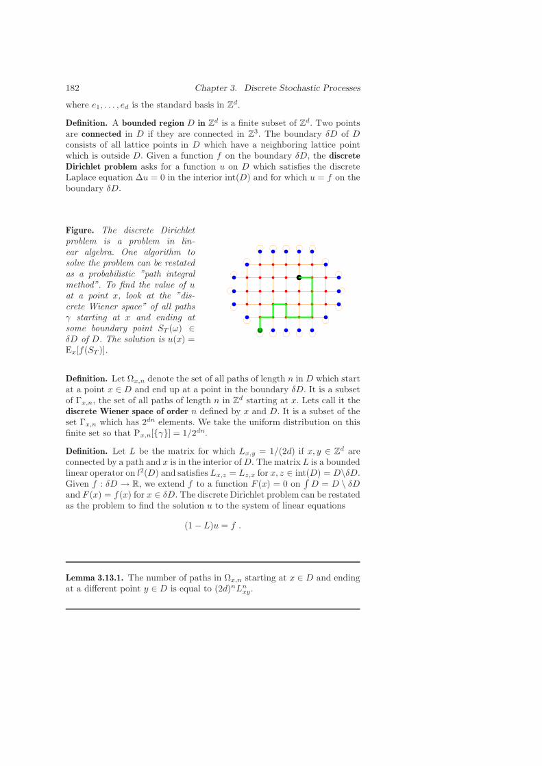
182 Chapter 3. Discrete Stochastic Processes
where e1, . . . , ed is the standard basis in Zd.
Definition. A bounded region D in Zd is a finite subset of Zd. Two pointsare connected in D if they are connected in Z3. The boundary δD of Dconsists of all lattice points in D which have a neighboring lattice pointwhich is outside D. Given a function f on the boundary δD, the discreteDirichlet problem asks for a function u on D which satisfies the discreteLaplace equation ∆u = 0 in the interior int(D) and for which u = f on theboundary δD.
Figure. The discrete Dirichletproblem is a problem in lin-ear algebra. One algorithm tosolve the problem can be restatedas a probabilistic ”path integralmethod”. To find the value of uat a point x, look at the ”dis-crete Wiener space” of all pathsγ starting at x and ending atsome boundary point ST (ω) ∈δD of D. The solution is u(x) =Ex[f(ST )].
Definition. Let Ωx,n denote the set of all paths of length n in D which startat a point x ∈ D and end up at a point in the boundary δD. It is a subsetof Γx,n, the set of all paths of length n in Zd starting at x. Lets call it thediscrete Wiener space of order n defined by x and D. It is a subset of theset Γx,n which has 2dn elements. We take the uniform distribution on thisfinite set so that Px,n[γ] = 1/2dn.
Definition. Let L be the matrix for which Lx,y = 1/(2d) if x, y ∈ Zd areconnected by a path and x is in the interior ofD. The matrix L is a boundedlinear operator on l2(D) and satisfies Lx,z = Lz,x for x, z ∈ int(D) = D\δD.Given f : δD → R, we extend f to a function F (x) = 0 on
∫
D = D \ δDand F (x) = f(x) for x ∈ δD. The discrete Dirichlet problem can be restatedas the problem to find the solution u to the system of linear equations
(1 − L)u = f .
Lemma 3.13.1. The number of paths in Ωx,n starting at x ∈ D and endingat a different point y ∈ D is equal to (2d)nLnxy.

3.13. Discrete Dirichlet problem 183
Proof. Use induction. By definition, Lxz is 1/(2d) if there is a path from xto z. The integer Lnx,y is the number of paths of length n from x to y.
Figure. Here is an example of aproblem where D ⊂ Z2 has 10points:
4L =
0 0 0 0 0 0 0 0 0 00 0 0 0 0 0 0 0 0 00 0 0 0 0 0 0 0 0 01 0 1 0 1 0 0 1 0 00 1 0 1 0 1 0 0 1 00 0 0 0 0 0 0 0 0 00 0 0 0 0 0 0 0 0 00 0 0 1 0 1 0 0 1 10 0 0 0 0 0 0 0 0 00 0 0 0 0 0 0 0 0 0
.
Only the rows corresponding tointerior points are nonzero.
Definition. For a function f on the boundary δD, define
Ex,n[f ] =∑
y∈δDf(y)Lnx,y
and
Ex[f ] =
∞∑
n=0
Ex,n[f ] .
This functional defines for every point x ∈ D a probability measure µx onthe boundary δD. It is the discrete analog of the harmonic measure in thecontinuum. The measure Px on the set of paths satisfies Ex[1] = 1 as wewill just see.
Proposition 3.13.2. Let Sn be the random walk on Zd and let T be thestopping time which is the first exit time of S from D. The solution to thediscrete Dirichlet problem is
u(x) = Ex[f(ST )] .
Proof. Because (1 − L)u = f and
Ex,n[f ] = (Lnf)x ,

184 Chapter 3. Discrete Stochastic Processes
we have from the geometric series formula
(1 −A)−1 =
n∑
k=0
Ak
the result
u(x) = (1 − L)−1f(x) =
∞∑
n=0
[Lnf ]x =
∞∑
n=0
Ex,n[f ] = Ex[ST ] .
Define the matrix K by Kjj = 1 for j ∈ δD and Kij = Lji/4 else. Thematrix K is a stochastic matrix: its column vectors are probability vectors.The matrix K has a maximal eigenvalue 1 and so norm 1 (KT has themaximal eigenvector (1, 1, . . . , 1) with eigenvalue 1 and since eigenvalues ofK agree with eigenvalues of KT ). Because ||L|| < 1, the spectral radius ofL is smaller than 1 and the series converges. If f = 1 on the boundary,then u = 1 everywhere. From Ex[1] = 1 follows that the discrete Wienermeasure is a probability measure on the set of all paths starting at x.
Figure. The randomwalk defines a diffu-sion process.
Figure. The diffusionprocess after time t =2.
Figure. The diffusionprocess after time t =3.
The path integral result can be generalized and the increased generalitymakes it even simpler to describe:
Definition. Let (D,E) be an arbitrary finite directed graph, where D isa finite set of n vertices and E ⊂ D × D is the set of edges. Denote anedge connecting i with j with eij . Let K be a stochastic matrix on l2(D):the entries satisfy Kij ≥ 0 and its column vectors are probability vectors∑
i∈DKij = 1 for all j ∈ D. The stochastic matrix encodes the graph andadditionally defines a random walk on D if Kij is interpreted as the tran-sition probability to hop from j to i. Lets call a point j ∈ δD a boundarypoint, ifKjj = 1. The complement intD = D\δD consists of interior points.Define the matrix L as Ljj = 0 if j is a boundary point and Lij = Kji
otherwise.
3.13. Discrete Dirichlet problem 185
The discrete Wiener space Ωx ⊂ D on D is the set of all finite paths γ =(x = x0, x1, x2, . . . , xn) starting at a point x ∈ D for which Kxixi+1 > 0.The discrete Wiener measure on this countable set is defined as Px[γ] =∏n−1j=0 Kj,j+1. A function u on D is called harmonic if (Lu)x = 0 for all
x ∈ D. The discrete Dirichlet problem on the graph is to find a function uon D which is harmonic and which satisfies u = f on the boundary δD ofD.
Theorem 3.13.3 (The Dirichlet problem on graphs). Assume D is a directedgraph. If Sn is the random walk starting at x and T is the stopping timeto reach the boundary of D, then the solution
u = Ex[f(ST )]
is the expected value of ST on the discrete Wiener space of all paths startingat x and ending at the boundary of D.
Proof. Let F be the function on D which agrees with f on the boundary ofD and which is 0 in the interior of D. The Dirichlet problem on the graphis the system of linear equations (1 − L)u = f . Because the matrix L hasspectral radius smaller than 1, the problem is given by the geometric series
u =
∞∑
n=0
Lnf .
But this is the sum Ex[f(ST )] over all paths γ starting at x and ending atthe boundary of f .
Example. Lets look at a directed graph (D,E) with 5 vertices and 2 bound-ary points. The Laplacian on D is defined by the stochastic matrix
K =
0 1/3 0 0 01/2 0 1 0 01/4 1/2 0 0 01/8 1/6 0 1 01/8 0 0 0 1
or the Laplacian
L =
0 1/2 1/4 1/8 1/81/3 0 1/2 1/6 00 1 0 0 00 0 0 1 00 0 0 0 1
.
Given a function f on the boundary of D, the solution u of the discreteDirichlet problem (1 − L)u = f on this graph can be written as a path

186 Chapter 3. Discrete Stochastic Processes
integral∑∞n=0 L
nf = Ex[f(ST )] for the random walk Sn on D stopped atthe boundary δD.
Figure. The directed graph(D,E) with 5 vertices and 2boundary points.
Remark. The interplay of random walks on graphs and discrete partialdifferential equations is relevant in electric networks. For mathematicaltreatments, see [19, 99].
3.14 Markov processes
Definition. Given a measurable space (S,B) called state space, where S isa set and B is a σ-algebra on S. A function P : S × B → R is called atransition probability function if P (x, ·) is a probability measure on (S,B)for all x ∈ S and if for every B ∈ B, the map s→ P (s,B) is B-measurable.Define P 1(x,B) = P (x,B) and inductively the measures Pn+1(x,B) =∫
S Pn(y,B)P (x, dy), where we write
∫
P (x, dy) for the integration on Swith respect to the measure P (x, ·).
Example. If S is a finite set and B is the set of all subsets of S. Givena stochastic matrix K and a point s ∈ S, the measures P (s, ·) are theprobability vectors, which are the columns of K.
Remark. The transition probability functions are elements in L(S,M1(S)),where M1(S) is the set of Borel probability measures on S. With the mul-tiplication
(P Q)(x,B) =
∫
S
P (y,B) dQ(x)
we get a commutative semi-group. The relation Pn+m = Pn Pm is alsocalled the Chapmann-Kolmogorov equation.
Definition. Given a probability space (Ω,A,P) with a filtration An of σ-algebras. An An-adapted process Xn with values in S is called a discrete

3.14. Markov processes 187
time Markov process if there exists a transition probability function P suchthat
P[Xn ∈ B | Ak](ω) = Pn−k(Xk(ω), B) .
Definition. If the state space S is a discrete space, a finite or countableset, then the Markov process is called a Markov chain, A Markov chain iscalled a denumerable Markov chain, if the state space S is countable, afinite Markov chain, if the state space is finite.
Remark. It follows from the definition of a Markov process thatXn satisfiesthe elementary Markov property: for n > k,
P[Xn ∈ B | X1, . . . , Xk] = P[Xn ∈ B | Xk] .
This means that the probability distribution of Xn is determined by know-ing the probability distribution of Xn−1. The future depends only on thepresent and not on the past.
Theorem 3.14.1 (Markov processes exist). For any state space (S,B) andany transition probability function P , there exists a corresponding Markovprocess X .
Proof. Choose a probability measure µ on (S,B) and define on the prod-uct space (Ω,A) = (SN,BN) the π-system C consisting of of cylinder-sets∏
n∈N Bn given by a sequence Bn ∈ B such that Bn = S except for finitelymany n. Define a measure P = Pµ on (Ω, C) by requiring
P[ωk ∈ Bk, k = 1, . . . n] =
∫
B0
µ(dx0)
∫
B1
P (x0, dx1) . . .
∫
Bn
P (xn−1, dxn) .
This measure has a unique extension to the σ-algebra A.Define the increasing sequence of σ-algebras An = Bn × ∏n
i=1∅,Ω con-taining cylinder sets. The random variables Xn(ω) = xn are An-adapted.In order to see that it is a Markov process, we have to check that
P[Xn ∈ Bn | An−1](ω) = P (Xn−1(ω), Bn)
which is a special case of the above requirement by taking Bk = S fork 6= n.
Example. Independent S-valued random variablesAssume the measures P (x, ·) are independent of x. Call this measure P. Inthis case
P[Xn ∈ Bn | An−1](ω) = P[Bn]

188 Chapter 3. Discrete Stochastic Processes
which means that P[Xn ∈ Bn | An−1] = P[Xn ∈ Bn]. The S− valuedrandom variables Xn are independent and have identical distribution andP is the law of Xn. Every sequence of IID random variables is a Markovprocess.
Example. Countable and finite state Markov chains.Given a Markov process with finite or countable state space S. We definethe transition matrix Pij on the Hilbert space l2(S) by
Pij = P (i, j) .The matrix P transports the law of Xn into the law of Xn+1.The transition matrix Pij is a stochastic matrix: each column is a proba-bility vector:
∑
j Pij = 1 with Pij ≥ 0. Every measure on S can be given
by a vector π ∈ l2(S) and Pπ is again a measure. If X0 is constant andequal to i and Xn is a Markov process with transition probability P , thenPnij = P[Xn = j].
Example. Sum of independent S-valued random variables Let S be a count-able Abelian group and let π be a probability distribution on S assigningto each j ∈ S the weight πj . Define Pij = πj−i. Now Xn is the sum of nindependent random variables with law π. The sum changes from i to jwith probability Pij = pi−j .
Example. Branching processes Given S = 0, 1, 2 . . . = N with fixedprobability distribution π. If X is a S-valued random variable with distri-bution π then
∑nk=1Xk has a distribution which we denote by π(n). Define
the matrix Pij = π(i)j . The Markov chain with this transition probability
matrix on S is called a branching process.
Definition. The transition probability function P acts also on measures πof S by
P(π)(B) =
∫
S
P (x,B) dπ(x) .
A probability measure π is called invariant if Pπ = π. An invariant measureπ on S is called stationary measure of the Markov process.
This operator on measures leaves a subclass of measures with densities withrespect to some measure ν invariant. We can so assign a Markov operatorto a transition probability function:
Lemma 3.14.2. For any x ∈ S define the measure
ν(B) =∞∑
n=0
1
2nPn(x,B)
on (S,B) has the property that if µ is absolutely continuous with respectto ν, then also Pµ is absolutely continuous with respect to ν.

3.14. Markov processes 189
Proof. Given µ = f · ν with f ∈ L1(S). Then
Pµ =
∫
S
P (x,B)f(x) dν(x)
is absolutely continuous with respect to ν because Pµ(B) = 0 impliesP (x,B) = 0 for almost all x with f(x) > 0 and so fν(B) = 0.
Corollary 3.14.3. To each transition probability function can be assigned aMarkov operator P : L1(S, ν) → L1(S, ν).
Proof. Choose ν as above and define
Pf1 = f2
if Pµ1 = µ2 with µi = fiνi. To check that P is a Markov operator, we haveto check Pf ≥ 0 if f ≥ 0, which follows from
Pfν(B) =
∫
S
P (x,B)f(x) dν(x) ≥ 0 .
We also have to show that ||Pf ||1 = 1 if ||f ||1. It is enough to show thisfor elementary functions f =
∑
j aj1Bj with aj > 0 with Bj ∈ B satisfying∑
j ajν(Bj) = 1 satisfies ||P1Bν|| = ν(B). But this is obvious ||P1Bν|| =∫
BP (x, ·) dν(x) = ν(B).
We see that the abstract approach to study Markov operators on L1(S) ismore general, than looking at transition probability measures. This pointof view can reduce some of the complexity, when dealing with discrete timeMarkov processes.

190 Chapter 3. Discrete Stochastic Processes

Chapter 4
Continuous StochasticProcesses
4.1 Brownian motion
Definition. Let (Ω,A,P) be a probability space and let T ⊂ R be time.A collection of random variables Xt, t ∈ T with values in R is called astochastic process. If Xt takes values in S = Rd, it is called a vector-valuedstochastic process but one often abbreviates this by the name stochasticprocess too. If the time T can be a discrete subset of R, then Xt is calleda discrete time stochastic process. If time is an interval, R+ or R, it iscalled a stochastic process with continuous time. For any fixed ω ∈ Ω, onecan regard Xt(ω) as a function of t. It is called a sample function of thestochastic process. In the case of a vector-valued process, it is a samplepath, a curve in Rd.
Definition. A stochastic process is called measurable, if X : T × Ω → S ismeasurable with respect to the product σ-algebra B(T )×A. In the case ofa real-valued process (S = R), one says X is continuous in probability iffor any t ∈ R the limit Xt+h → Xt takes place in probability for h → 0.If the sample function Xt(ω) is a continuous function of t for almost all ω,then Xt is called a continuous stochastic process. If the sample function isa right continuous function in t for almost all ω ∈ Ω, Xt is called a rightcontinuous stochastic process. Two stochastic process Xt and Yt satisfyingP[Xt − Yt = 0] = 1 for all t ∈ T are called modifications of each otheror indistinguishable. This means that for almost all ω ∈ Ω, the samplefunctions coincide Xt(ω) = Yt(ω).
Definition. A Rn-valued random vector X is called Gaussian, if it has themultidimensional characteristic function
φX(s) = E[eis·X ] = e−(s,V s)/2+i(m,s)
191

192 Chapter 4. Continuous Stochastic Processes
for some nonsingular symmetric n×n matrix V and vector m = E[X ]. Thematrix V is called covariance matrix and the vector m is called the meanvector.
Example. A normal distributed random variable X is a Gaussian randomvariable. The covariance matrix is in this case the scalar Var[X ].
Example. If V is a symmetric matrix with determinant det(V ) 6= 0, thenthe random variable
X(x) =1
(2π)n/2√
det(V )e−(x−m,V−1(x−m))/2
on Ω = Rn is a Gaussian random variable with covariance matrix V . Tosee that it has the required multidimensional characteristic function φX(u).Note that because V is symmetric, one can diagonalize it. Therefore, thecomputation can be done in a bases, where V is diagonal. This reduces thesituation to characteristic functions for normal random variables.
Example. A set of random variables X1, . . . , Xn are called jointly Gaussianif any linear combination
∑ni=1 aiXi is a Gaussian random variable too.
For a jointly Gaussian set of of random variables Xj, the vector X =(X1, . . . , Xn) is a Gaussian random vector.
Example. A Gaussian process is a Rd-valued stochastic process with con-tinuous time such that (Xt0 , Xt1 , . . . , Xtn) is jointly Gaussian for any t0 ≤t1 < · · · < tn. It is called centered if mt = E[Xt] = 0 for all t.
Definition. An Rd-valued continuous Gaussian processXt with mean vectormt = E[Xt] and the covariance matrix V (s, t) = Cov[Xs, Xt] = E[(Xs −ms)·(Xt−mt)
∗] is called Brownian motion if for any 0 ≤ t0 < t1 < · · · < tn,the random vectors Xt0 , Xti+1 − Xti are independent and the covariancematrix V satisfies V (s, t) = V (r, r), where r = min(s, t) and s 7→ V (s, s).It is called the standard Brownian motion if mt = 0 for all t and V (s, t) =mins, t.
Figure. A path Xt(ω1) of Brow-nian motion in the plane S = R2
with a drift mt = E[Xt] = (t, 0).This is not standard Brownianmotion. The process Yt = Xt −(t, 0) is standard Brownian mo-tion.

4.1. Brownian motion 193
Recall that for two random vectorsX,Y with mean vectorsm,n, the covari-ance matrix is Cov[X,Y ]ij = E[(Xi−mi)(Yj −nj)]. We say Cov[X,Y ] = 0if this matrix is the zero matrix.
Lemma 4.1.1. A Gaussian random vector (X,Y ) with random vectors X,Ysatisfying Cov[X,Y ] = 0 has the property that X and Y are independent.
Proof. We can assume without loss of generality that the random variablesX,Y are centered. Two Rn-valued Gaussian random vectors X and Y areindependent if and only if
φ(X,Y )(s, t) = φX(s) · φY (t), ∀s, t ∈ Rn
Indeed, if V is the covariance matrix of the random vector X and W is thecovariance matrix of the random vector Y , then
U =
[
U Cov[X,Y ]Cov[Y,X ] V
]
=
[
U 00 V
]
is the covariance matrix of the random vector (X,Y ). With r = (t, s), wehave therefore
φ(X,Y )(r) = E[eir·(X,Y )] = e−12 (r·Ur)
= e−12 (s·V s)− 1
2 (t·Wt)
= e−12 (s·V s)e−
12 (t·Wt)
= φX(s)φY (t) .
Example. In the context of this lemma, one should mention that thereexist uncorrelated normal distributed random variables X,Y which are notindependent [109]: Proof. Let X be Gaussian on R and define for α > 0 thevariable Y (ω) = −X(ω), if ω > α and Y = X else. Also Y is Gaussian andthere exists α such that E[XY ] = 0. But X and Y are not independent andX+Y = 0 on [−α, α] shows thatX+Y is not Gaussian. This example showswhy Gaussian vectors (X,Y ) are defined directly as R2 valued randomvariables with some properties and not as a vector (X,Y ) where each ofthe two component is a one-dimensional random Gaussian variable.
Proposition 4.1.2. If Xt is a Gaussian process with covariance V (s, t) =V (r, r) with r = min(s, t), then it is Brownian motion.

194 Chapter 4. Continuous Stochastic Processes
Proof. By the above lemma (4.1.1), we only have to check that for all i < j
Cov[Xt0 , Xtj+1 −Xtj ] = 0, Cov[Xti+1 −Xti , Xtj+1 −Xtj ] = 0 .
But by assumption
Cov[Xt0 , Xtj+1 −Xtj ] = V (t0, tj+1) − V (t0, tj) = V (t0, t0) − V (t0, t0) = 0
and
Cov[Xti+1 −Xti , Xtj+1 −Xtj ] = V (ti+1, tj+1) − V (ti+1, tj)
−V (ti, tj+1) + V (ti, tj)
= V (ti+1, ti+1) − V (ti+1, ti+1)
−V (ti, ti) + V (ti, ti) = 0 .
Remark. Botanist Robert Brown was studying the fertilization process in aspecies of flowers in 1828. While watching pollen particles in water througha microscope, he observed small particles in ”rapid oscillatory motion”.While previous studies concluded that these particles were alive, Brown’sexplanation was that matter is composed of small ”active molecules”, whichexhibit a rapid, irregular motion having its origin in the particles themselvesand not in the surrounding fluid. Brown’s contribution was to establishBrownian motion as an important phenomenon, to demonstrate its presencein inorganic as well as organic matter and to refute by experiment incorrectmechanical or biological explanations of the phenomenon. The book [73]includes more on the history of Brownian motion.
The construction of Brownian motion happens in two steps: one first con-structs a Gaussian process which has the desired properties and then showsthat it has a modification which is continuous.
Proposition 4.1.3. Given a separable real Hilbert space (H, || · ||). Thereexists a probability space (Ω,A,P) and a family X(h), h ∈ H of real-valuedrandom variables on Ω such that h 7→ X(h) is linear, and X(h) is Gaussian,centered and E[X(h)2] = ||h||2.
Proof. Pick an orthonormal basis en in H and attach to each en a cen-tered Gaussian IID random variable Xn ∈ L2 satisfying ||Xn||2 = 1. Givena general h =
∑
hnen ∈ H , define
X(h) =∑
n
hnXn
which converges in L2. Because Xn are independent, they are orthonormalin L2 so that
||X(h)||22 =∑
n
h2n||Xn||2 =
∑
n
h2n = ||h||22 .

4.1. Brownian motion 195
Definition. If we choose H = L2(R+, dx), the map X : H 7→ L2 isalso called a Gaussian measure. For a Borel set A ⊂ R+ we define thenX(A) = X(1A). The term ”measure” is warranted by the fact that X(A) =∑
nX(An) if A is a countable disjoint union of Borel sets An. One also hasX(∅) = 0.
Remark. The space X(H) ⊂ L2 is a Hilbert space isomorphic to H and inparticular
E[X(h)X(h′)] = (h, h′) .
We know from the above lemma that h and h′ are orthogonal if and onlyif X(h) and X(h′) are independent and that
E[X(A)X(B)] = Cov[X(A), X(B)] = (1A, 1B) = |A ∩B| .
Especially X(A) and X(B) are independent if and only if A and B aredisjoint.
Definition. Define the process Bt = X([0, t]). For any sequence t1, t2, · · · ∈T , this process has independent increments Bti −Bti−1 and is a Gaussianprocess. For each t, we have E[B2
t ] = t and for s < t, the increment Bt−Bshas variance t− s so that
E[BsBt] = E[B2s ] + E[Bs(Bt −Bs)] = E[B2
s ] = s .
This model of Brownian motion has everything except continuity.
Theorem 4.1.4 (Kolmogorov’s lemma). Given a stochastic process Xt witht ∈ [a, b] for which there exist three constants p > r,K such that
E[|Xt+h −Xt|p] ≤ K · h1+r
for every t, t + h ∈ [a, b], then Xt has a modification Yt which is almosteverywhere continuous: for all s, t ∈ [a, b]
|Yt(ω) − Ys(ω)| ≤ C(ω) |t− s|α, 0 < α <r
p.
Proof. We can assume without loss of generality that a = 0, b = 1 becausewe can translate and rescale the time variable to be in this situation. Defineǫ = r − αp. By the Chebychev-Markov inequality (2.5.4)
P[|Xt+h −Xt|] ≥ |h|α] ≤ |h|−αpE[|Xt+h −Xt|p] ≤ K|h|1+ǫ
so thatP[|X(k+1)/2n −Xk/2n | ≥ 2−nα] ≤ K2−n(1+ǫ) .

196 Chapter 4. Continuous Stochastic Processes
Therefore
∞∑
n=1
2n−1∑
k=0
P[|X(k+1)/2n −Xk/2n | ≥ 2−nα] <∞ .
By the first Borel-Cantelli’s lemma (2.2.2), there exists n(ω) < ∞ almosteverywhere such that for all n ≥ n(ω) and k = 0, . . . , 2n − 1
|X(k+1)/2n(ω) −Xk/2n(ω)| < 2−nα .
Let n ≥ n(ω) and t ∈ [k/2n, (k+1)/2n] of the form t = k/2n+∑mi=1 γi/2
n+i
with γi ∈ 0, 1. Then
|Xt(ω) −Xk2−n(ω)| ≤m
∑
i=1
γi2−α(n+i) ≤ d 2−nα
with d = (1 − 2−α)−1. Similarly
|Xt −X(k+1)2−n | ≤ d 2−nα .
Given t, t + h ∈ D = k2−n | n ∈ N, k = 0, . . . n − 1. Take n so that2−n−1 ≤ h < 2−n and k so that k/2n+1 ≤ t < (k + 1)/2n+1. Then (k +1)/2n+1 ≤ t+ h ≤ (k + 3)/2n+1 and
|Xt+h −Xt| ≤ 2d2−(n+1)α ≤ 2dhα .
For almost all ω, this holds for sufficiently small h.
We know now that for almost all ω, the path Xt(ω) is uniformly continuouson the dense set of dyadic numbers D = k/2n. Such a function can beextended to a continuous function on [0, 1] by defining
Yt(ω) = lims∈D→t
Xs(ω) .
Because the inequality in the assumption of the theorem implies E[Xt(ω)−lims∈D→tXs(ω)] = 0 and by Fatou’s lemma E[Yt(ω)−lims∈D→tXs(ω)] = 0we know that Xt = Yt almost everywhere. The process Y is therefore amodification of X . Moreover, Y satisfies
|Yt(ω) − Ys(ω)| ≤ C(ω) |t− s|α
for all s, t ∈ [a, b].
Corollary 4.1.5. Brownian motion exists.

4.1. Brownian motion 197
Proof. In one dimension, take the process Bt from above. Since Xh =Bt+h − Bt is centered with variance h, the fourth moment is E[X4
h] =d4
dx4 exp(−x2h/2)|x=0 = 3h2, so that
E[(Bt+h −Bt)4] = 3h2 .
Kolmogorov’s lemma (4.1.4) assures the existence of a continuous modifi-cation of B.
To define standard Brownian motion in n dimension, we take the joint
motion Bt = (B(1)t , . . . , B
(n)t ) of n independent one- dimensional Brownian
motions.
Definition. Let Bt be the standard Brownian motion. For any x ∈ Rn, theprocess Xx
t = x+Bt is called Brownian motion started at x.
The first rigorous construction of Brownian motion was given by NorbertWiener in 1923. By construction of a Wiener measure on C[0, 1], one hasa construction of Brownian motion, where the probability space is directlygiven by the set of paths. One has then the process Xt(ω) = ω(t). We willcome to this later. A general construction of such measures is possible givena Markov transition probability function [104]. The construction given hereis due to Neveu and goes back to Kakutani. It can be found in Simon’s bookon functional integration [93] or in the book of Revuz and Yor [83] aboutcontinuous martingales and Brownian motion. This construction has theadvantage that it can be applied to more general situations.
In McKean’s book ”Stochastic integrals” [66] one can find Levy’s directproof of the existence of Brownian motion. Because that proof gives an ex-plicit formula for the Brownian motion process Bt and is so constructive,we outline it shortly:
1) Take as a basis in L2([0, 1] the Haar functions
fk,n := 2(n−1)/2(1[(k−1)2−n,k2−n] − 1[k2−n,(k+1)2−n])
for (k, n)|n ≥ 1, k < 2n and f0,0 = 1.
2) Take a family Xk,n for (k, n) ∈ I = (k, n) | n ≥ 1, k < 2n, k odd ∪(0, 0) of independent Gaussian random variables.
3) Define
Bt =∑
(k,n)∈IXk,n
∫ t
0
fk,n .
4) Prove convergence of the above series.
5) Check
E[BsBt] =∑
(k,n)∈I
∫ s
0
∫ t
0
f(k,n)fι =
∫ 1
0
1[0,s]1[0,t] = infs, t .

198 Chapter 4. Continuous Stochastic Processes
6) Extend the definition from t ∈ [0, 1] to t ∈ [0,∞) by taking independent
Brownian motions B(i)t and defining Bt =
∑
n<[t]B(n)t−n, where [t] is the
largest integer smaller or equal to t.
4.2 Some properties of Brownian motion
We first want to establish that Brownian motion is unique. To do so, wefirst have to say, when two processes are the same:
Definition. Two processes Xt on (Ω,A,P) and X ′t on (Ω′,A′,P′) are called
indistinguishable, if there exists an isomorphism U : Ω → Ω′ of probabilityspaces, such that X ′
t(Uω) = Xt(ω). Indistinguishable processes are consid-ered the same. A special case is if the two processes are defined on the sameprobability space (Ω,A,P) and Xt(ω) = Yt(ω) for almost all ω.
Proposition 4.2.1. Brownian motion is unique in the sense that two stan-dard Brownian motions are indistinguishable.
Proof. The construction of the map H → L2 was unique in the sense thatif we construct two different processes X(h) and Y (h), then there exists anisomorphism U of the probability space such that X(h) = Y (U(h)). Thecontinuity of Xt and Yt implies then that for almost all ω, Xt(ω) = Yt(Uω).In other words, they are indistinguishable.
We are now ready to list some symmetries of Brownian motion.
Theorem 4.2.2 (Properties of Brownian motion). The following symmetriesexist:(i) Time-homogeneity: For any s > 0, the process Bt = Bt+s − Bs is aBrownian motion independent of σ(Bu, u ≤ s).(ii) Reflection symmetry: The process Bt = −Bt is a Brownian motion.(iii) Brownian scaling: For every c > 0, the process Bt = cBt/c2 is a Brow-nian motion.(iv) Time inversion: The process B0 = 0, Bt = tB1/t, t > 0 is a Brownianmotion.
Proof. (i),(ii),(iii) In each case, Bt is a continuous centered Gaussian pro-cess with continuous paths, independent increments and variance t.
4.2. Some properties of Brownian motion 199
(iv) B is a centered Gaussian process with covariance
Cov[Bs, Bt] = E[Bs, Bt] = st · E[B1/s, B1/t] = st · inf(1
s,1
t) = inf(s, t) .
Continuity of Bt is obvious for t > 0. We have to check continuity only fort = 0, but since E[B2
s ] = s → 0 for s → 0, we know that Bs → 0 almosteverywhere.
It follows the strong law of large numbers for Brownian motion:
Theorem 4.2.3 (SLLN for Brownian motion). If Bt is Brownian motion,then
limt→∞
1
tBt = 0
almost surely.
Proof. From the time inversion property (iv), we see that t−1Bt = B1/t
which converges for t → ∞ to 0 almost everywhere, because of the almosteverywhere continuity of Bt.
Definition. A parameterized curve t ∈ [0,∞) 7→ Xt ∈ Rn is called Holdercontinuous of order α if there exists a constant C such that
||Xt+h −Xt|| ≤ C · hα
for all h > 0 and all t. A curve which is Holder continuous of order α = 1is called Lipshitz continuous.
The curve is called locally Holder continuous of order α if there exists foreach t a constant C = C(t) such that
||Xt+h −Xt|| ≤ C · hα
for all small enough h. For a Rd-valued stochastic process, (local) Holdercontinuity holds if for almost all ω ∈ Ω the sample path Xt(ω) is (local)Holder continuous for almost all ω ∈ Ω.
Proposition 4.2.4. For every α < 1/2, Brownian motion has a modificationwhich is locally Holder continuous of order α.

200 Chapter 4. Continuous Stochastic Processes
Proof. It is enough to show it in one dimension because a vector func-tion with locally Holder continuous component functions is locally Holdercontinuous. Since increments of Brownian motion are Gaussian, we have
E[(Bt −Bs)2p] = Cp · |t− s|p
for some constant Cp. Kolmogorov’s lemma assures the existence of a mod-ification satisfying locally
|Bt −Bs| ≤ C |t− s|α, 0 < α <p− 1
2p.
Because p can be chosen arbitrary large, the result follows.
Because of this proposition, we can assume from now on that all the pathsof Brownian motion are locally Holder continuous of order α < 1/2.
Definition. A continuous path Xt = (X(1)t , . . . , X
(n)t ) is called nowhere
differentiable, if for all t, each coordinate function X(i)t is not differentiable
at t.
Theorem 4.2.5 (Wiener). Brownian motion is nowhere differentiable: foralmost all ω, the path t 7→ Xt(ω) is nowhere differentiable.
Proof. We follow [66]. It is enough to show it in one dimensions. SupposeBt is differentiable at some point 0 ≤ s ≤ 1. There exists then an integer lsuch that |Bt − Bs| ≤ l(t− s) for t− s > 0 small enough. But this meansthat
|Bj/n −B(j−1)/n| ≤ 7l
n
for all j satisfying
i = [ns] + 1 ≤ j ≤ [ns] + 4 = i+ 3
and sufficiently large n so that the set of differentiable paths is included inthe set
B =⋃
l≥1
⋃
m≥1
⋂
n≥m
⋃
0<i≤n+1
⋂
i<j≤i+3
|Bj/n −B(j−1)/n| < 7l
n .

4.2. Some properties of Brownian motion 201
Using Brownian scaling, we show that P[B] = 0 as follows
P[⋂
n≥m
⋃
0<i≤n+1
⋂
i<j≤i+3
|Bj/n −B(j−1)/n| < 7l
n]
≤ lim infn→∞
nP[|B1/n| < 7l
n]3
= lim infn→∞
nP[|B1| < 7l√n
]3
≤ limn→∞
C√n
= 0 .
Remark. This proposition shows especially that we have no Lipshitz con-tinuity of Brownian paths. A slight generalization shows that Brownianmotion is not Holder continuous for any α ≥ 1/2. One has just to do thesame trick with k instead of 3 steps, where k(α − 1/2) > 1. The actualmodulus of continuity is very near to α = 1/2: |Bt −Bt+ǫ| is of the order
h(ǫ) =
√
2ǫ log(1
ǫ) .
More precisely, P[lim supǫ→0 sup|s−t|≤ǫ|Bs−Bt|h(ǫ) = 1] = 1, as we will see
later in theorem (4.4.2).The covariance of standard Brownian motion was given by E[BsBt] =mins, t. We constructed it by implementing the Hilbert space L2([0,∞))as a Gaussian subspace of L2(Ω,A,P). We look now at a more general classof Gaussian processes.
Definition. A function V : T × T → R is called positive semidefinite,if for all finite sets t1, . . . , td ⊂ T , the matrix Vij = V (ti, tj) satisfies(u, V u) ≥ 0 for all vectors u = (u1, . . . , un).
Proposition 4.2.6. The covariance of a centered Gaussian process is positivesemidefinite. Any positive semidefinite function V on T×T is the covarianceof a centered Gaussian process Xt.
Proof. The first statement follows from the fact that for all u = (u1, . . . , un)
∑
i,j
V (ti, tj)uiuj = E[(n
∑
i=1
uiXti)2] ≥ 0 .
We introduce for t ∈ T a formal symbol δt. Consider the vector space offinite sums
∑ni=1 aiδti with inner product
(d
∑
i=1
aiδti ,d
∑
j=1
bjδtj ) =∑
i,j
aibjV (ti, tj) .
202 Chapter 4. Continuous Stochastic Processes
This is a positive semidefinite inner product. Multiplying out the null vec-tors ||v|| = 0 and doing a completion gives a separable Hilbert spaceH . Define now as in the construction of Brownian motion the processXt = X(δt). Because the map X : H → L2 preserves the inner product, wehave
E[Xt, Xs] = (δs, δt) = V (s, t) .
Lets look at some examples of Gaussian processes:
Example. The Ornstein-Uhlenbeck oscillator processXt is a one-dimensionalprocess which is used to describe the quantum mechanical oscillator as wewill see later. Let T = R+ and take the function V (s, t) = 1
2e−|t−s| on
T ×T . We first show that V is positive semidefinite: The Fourier transformof f(t) = e−|t| is
∫
R
eikte−|t|dt =1
2π(k2 + 1).
By Fourier inversion, we get
1
2π
∫
R
(k2 + 1)−1eik(t−s) dk =1
2e−|t−s| ,
and so
0 ≤ (2π)−1
∫
R
(k2 + 1)−1∑
j
|ujeiktj |2 dk
=n
∑
j,k=1
ujuk1
2e−|tj−tk| .
This process has a continuous modification because
E[(Xt −Xs)2] = (e−|t−t| + e−|s−s| − 2e−|t−s|)/2 = (1 − e−|t−s|) ≤ |t− s|
and Kolmogorov’s criterion. The Ornstein-Uhlenbeck is also called the os-cillatory process.
Proposition 4.2.7. Brownian motion Bt and the Ornstein-Uhlenbeck pro-cess Ot are for t ≥ 0 related by
Ot =1√2e−tBe2t .
Proof. Denote by O the Ornstein-Uhlenbeck process and let
Xt = 2−1/2e−tBe2t .

4.2. Some properties of Brownian motion 203
We want to show that X = Y . Both X and O are centered Gaussian,continuous processes with independent increments. To verify that they arethe same, we have to show that they have the same covariance. This is acomputation:
E[OtOs] =1
2e−te−smine2t, e2s = e|s−t|/2 .
It follows from this relation that also the Ornstein-Uhlenbeck process isnot differentiable almost everywhere. There are also generalized Ornstein-Uhlenbeck processes. The case V (s, t) =
∫
Re−ik(t−s) dµ(k) = µ(t − s)
with the Cauchy measure µ = 12π(k2+1)dx on R can be generalized to take
any symmetric measure µ on R and let µ denote its Fourier transform∫
Re−ikt dµ(k). The same calculation as above shows that the function
V (s, t) = µ(t− s) is positive semidefinite.
Figure. Three paths of theOrnstein-Uhlenbeck process.
Example. Brownian bridge is a one-dimensional process with time T =[0, 1] and V (s, t) = s(1 − t) for 1 ≤ s ≤ t ≤ 1 and V (s, t) = V (t, s) else. Itis also called tied down process.
In order to show that V is positive semidefinite, one observes that Xt =Bs − sB1 is a Gaussian process, which has the covariance
E[XsXt] = E[(Bs − sB1)(Bt − tB1)] = s+ st− 2st = s(1 − t) .
Since E[X21 ] = 0, we have X1 = 0 which means that all paths start from 0
at time 0 and end at 1 at time 1.The realization Xt = Bs − sB1 shows also that Xt has a continuous real-ization.

204 Chapter 4. Continuous Stochastic Processes
Figure. Three paths of Brownianbridge.
Let Xt be the Brownian bridge and let y be a point in Rd. We can considerthe Gaussian process Yt = ty +Xt which describes paths going from 0 attime 0 to y at time 1. The process Y has however no more zero mean.Brownian motion B and Brownian bridge X are related to each other bythe formulas:
Bt = Bt := (t+ 1)Xt/(t+1), Xt = Xt := (1 − t)Bt/(1−t) .
These identities follow from the fact that both are continuous centeredGaussian processes with the right covariance:
E[BsBt] = (t+ 1)(s+ 1)min t
(t+ 1),
s
(s+ 1) = mins, t = E[BsBt] ,
E[XsXt] = (1 − t)(1 − s)min s
(1 − s),
t
(1 − t) = s(1 − t) = E[XsXt]
and uniqueness of Brownian motion.
Example. If V (s, t) = 1s=t , we get a Gaussian process which has theproperty that Xs and Xt are independent, if s 6= t. Especially, there is noautocorrelation between different Xs and Xt. This process is called whitenoise or ”great disorder”. It can not be modified so that (t, ω) 7→ Xt(ω) is
measurable: if (t, ω) 7→ Xt(ω) were measurable, then Yt =∫ t
0 Xs ds wouldbe measurable too. But then
E[Y 2t ] = E[(
∫ t
0
Xs)2] =
∫ t
0
∫ t′
0
E[Xs′Xs′ ] ds′ ds = 0
which implies Yt = 0 almost everywhere so that the measure dµ(ω) =Xs(ω) ds is zero for almost all ω.
t = E[
∫ t
0
X2s ] = E[
∫ t
0
XsXs ds] = E[
∫ t
0
Xs dµ(s)] = 0 .
In a distributional sense, one can see Brownian motion as a solution ofthe stochastic differential equation and white noise as a generalized mean-square derivative of Brownian motion. We will look at stochastic differentialequations later.

4.3. The Wiener measure 205
Example. Brownian sheet is not a stochastic process with one dimensionaltime but a random field: time T = R2
+ is two dimensional. Actually, aslong as we deal only with Gaussian random variables and do not want totackle regularity questions, the time T can be quite arbitrary and proposi-tion (4.2.6) stated at the beginning of this section holds true. The Gaussianprocess with
V ((s1, s2), (t1, t2)) = min(s1, t1) · min(s2, t2)
is called Brownian sheet. It has similar scaling properties as Brownian mo-tion.
Figure. Illustrating a sample of aBrownian sheet Bt,s. Time is twodimensional. Every trace Bt =Bt,s0 or Bt = Bt,s0 is standardBrownian motion.
4.3 The Wiener measure
Let (E, E) be a measurable space and let T be a set called ”time”. Astochastic process on a probability space (Ω,A,P) indexed by T and withvalues in E defines a map
φ : Ω → ET , ω 7→ Xt(ω) .
The product space ET is equipped with the product σ-algebra ET , whichis the smallest algebra for which all the functions Xt are measurable whichis the σ-algebra generated by the π-system
n
∏
t1,...,tn
Ati = x ∈ ET , xti ∈ Ati | Ati ∈ E
consisting of cylinder sets. Denote by Yt(w) = w(t) the coordinate maps onET . Because Yt φ is measurable for all t, also φ is measurable. Denote byPX the push-forward measure of φ from (Ω,A,P) to (ET , ET ) defined byPX [A] = P[X−1(A)]. For any finite set (t1, . . . , tn) ⊂ T and all sets Ai ∈ E ,we have
P[Xti ∈ Ai, i = 1, . . . , n] = PX [Yti ∈ Ai, 1 = 1, . . . n] .
One says, the two processes X and Y are versions of each other.

206 Chapter 4. Continuous Stochastic Processes
Definition. Y is called the coordinate process of X and the probabilitymeasure PX is called the law of X .
Definition. Two processes X,X ′ possibly defined on different probabilityspaces are called versions of each other if they have the same law PX = PX′ .
One usually does not work with the coordinate process but prefers to workwith processes which have some continuity properties. Many processes haveversions which are right continuous and have left hand limits at every point.
Definition. Let D be a measurable subset of ET and assume the process hasa versionX such that almost all pathsX(ω) are inD. Define the probabilityspace (D, ET ∩ D,Q), where Q is the measure Q = φ∗P. Obviously, theprocess Y defined on (D, ET ∩D,Q) is another version of X . If D is rightcontinuous with left hand limits, the process is called the canonical versionof X .
Corollary 4.3.1. Let E = Rd and T = R+. There exists a unique probabilitymeasure W on C(T,E) for which the coordinate process Y is the Brownianmotion B.
Proof. Let D = C(T,E) ⊂ ET . Define the measure W = φ∗PX and letY be the coordinate process of B. Uniqueness: assume we have two suchmeasures W,W ′ and let Y, Y ′ be the coordinate processes of B on D withrespect to W and W ′. Since both Y and Y ′ are versions of X and ”beinga version” is an equivalence relation, they are also versions of each other.This means that W and W ′ coincide on a π- system and are therefore thesame.
Definition. If E = Rd and T = [0,∞), the measure W on C(T,E) is calledthe Wiener measure. The probability space (C(T,E), ET ∩ C(T,E),W ) iscalled the Wiener space.
Let B′ be the σ-algebra ET ∩ C(T,E), which is the Borel σ-algebra re-stricted to C(T,E). The space C(T,E) carries an other σ-algebra, namelythe Borel σ-algebra B generated by its own topology. We have B ⊂ B′,since all closed balls f ∈ C(T,E) | |f − f0| ≤ r ∈ B are in B′. The otherrelation B′ ⊂ B is clear so that B = B′. The Wiener measure is therefore aBorel measure.
Remark. The Wiener measure can also be constructed without Brownianmotion and can be used to define Brownian motion. We sketch the idea.Let S = Rn denote the one point compactification of Rn. Define Ω = S[0,t]

4.4. Levy’s modulus of continuity 207
be the set of functions from [0, t] to S which is also the set of paths in Rn.
It is by Tychonov a compact space with the product topology. Define
Cfin(Ω) = φ ∈ C(Ω,R) | ∃F : Rn → R, φ(ω) = F (ω(t1), . . . , ω(tn)) .
Define also the Gauss kernel p(x, y, t) = (4πt)−n/2 exp(−|x−y|2/4t). Defineon Cfin(Ω) the functional
(Lφ)(s1, . . . , sm) =
∫
(Rn)m
F (x1, x2, . . . , xm)p(0, x1, s1)p(x1, x2, s2)
· · · p(xm−1, xm, sm) dx1 · · · dxm
with s1 = t1 and sk = tk − tk−1 for k ≥ 2. Since L(φ) ≤ |φ(ω)|∞, itis a bounded linear functional on the dense linear subspace Cfin(Ω) ⊂C(Ω). It is nonnegative and L(1) = 1. By the Hahn Banach theorem, itextends uniquely to a bounded linear functional on C(Ω). By the Rieszrepresentation theorem, there exists a unique measure µ on C(Ω) such thatL(φ) =
∫
φ(ω) dµ(ω). This is the Wiener measure on Ω.
4.4 Levy’s modulus of continuity
We start with an elementary estimate
Lemma 4.4.1.
1
ae−a
2/2 >
∫ ∞
a
e−x2/2 dx >
a
a2 + 1e−a
2/2 .
Proof.∫ ∞
a
e−x2/2 dx <
∫ ∞
a
e−x2/2(x/a) dx =
1
ae−a
2/2 .
For the right inequality consider
∫ ∞
a
1
b2e−b
2/2 db <1
a2
∫ ∞
a
e−x2/2 dx .
Integrating by parts of the left hand side of this gives
1
ae−a
2/2 −∫ ∞
a
e−x2/2 dx <
1
a2
∫ ∞
a
e−x2/2 dx .

208 Chapter 4. Continuous Stochastic Processes
Theorem 4.4.2 (Levy’s modulus of continuity). If B is standard Brownianmotion, then
P[lim supǫ→0
sup|s−t|≤ǫ
|Bs −Bt|h(ǫ)
= 1] = 1 ,
where h(ǫ) =√
2ǫ log(1/ǫ).
Proof. We follow [83]:
(i) Proof of the inequality ”≥ 1”.Take 0 < δ < 1. Define an = (1 − δ)h(2−n) = (1 − δ)
√n2 log 2. Consider
P[An] = P[ max1≤k≤2n
|Bk2−n −B(k−1)2−n | ≤ an] .
Because Bk/2n −B(k−1)/2n are independent Gaussian random variables, wecompute, using the above lemma (4.4.1) and 1 − s < e−s
P[An] ≤ (1 − 2
∫ ∞
an
1√2πe−x
2/2 dx)2n
≤ (1 − 2an
a2n + 1
e−a2n/2)2
n
≤ exp(−2n2ana2n + 1
e−a2n/2) ≤ e−C exp(n(1−(1−δ)2)/
√n) ,
where C is a constant independent of n. Since∑
n P[An] < ∞, we get bythe first Borel-Cantelli that P[lim supnAn] = 0 so that
P[ limn→∞
max1≤k≤2n
|Bk2−n −B(k−1)2n | ≥ h(2−n)] = 1 .
(ii) Proof of the inequality ”≤ 1”.Take again 0 < δ < 1 and pick ǫ > 0 such that (1 + ǫ)(1 − δ) > (1 + δ).Define
P[An] = P[ maxk=j−i∈K
|Bj2−n −Bi2−n |/h(k2−n) ≥ (1 + ǫ)]
= P[⋃
k=j−i∈K|Bj2−n −Bi2−n |] ≥ an,k ,
where
K = 0 < k ≤ 2nδ
and an,k = h(k2−n)(1 + ǫ).Using the above lemma, we get with some constants C which may vary

4.5. Stopping times 209
from line to line:
P[An] ≤∑
k∈Ka−1n,ke
−a2n,k/2
≤ C ·∑
k∈Klog(k−12n)−1/2e−(1+ǫ)2 log(k−12n)
≤ C · 2−n(1−δ)(1+ǫ)2 ∑
k∈K(log(k−12n))−1/2 ( since k−1 > 2−nδ)
≤ C · n−1/22n(δ−(1−δ)(1+ǫ)2) .
In the last step was used that there are at most 2nδ points in K and foreach of them log(k−12n) > log(2n(1 − δ)).We see that
∑
n P[An] converges. By Borel-Cantelli we get for almost everyω an integer n(ω) such that for n > n(ω)
|Bj2−n −Bi2−n | < (1 + ǫ) · h(k2−n) ,where k = j − i ∈ K. Increase possibly n(ω) so that for n > n(ω)
∑
m>n
h(2−m) < ǫ · h(2−(n+1)(1−δ)) .
Pick 0 ≤ t1 < t2 ≤ 1 such that t = t2 − t1 < 2−n(ω)(1−δ). Take nextn > n(ω) such that 2−(n+1)(1−δ) ≤ t < 2−n(1−δ) and write the dyadicdevelopment of t1, t2:
t1 = i2−n − 2−p1 − 2−p2 . . . , t2 = j2−n + 2−q1 + 2−q2 . . .
with t1 ≤ i2−n < j2−n ≤ t2 and 0 < k = j − i ≤ t2n < 2nδ. We get
|Bt1(ω) −Bt2(ω)| ≤ |Bt1 −Bi2−n(ω)|+|Bi2−n(ω) −Bj2−n(ω)|+|Bj2−n(ω) −Bt2 |
≤ 2∑
p>n
(1 + ǫ)h(2−p) + (1 + ǫ)h(k2−n)
≤ (1 + 3ǫ+ 2ǫ2)h(t) .
Because ǫ > 0 was arbitrary, the proof is complete.
4.5 Stopping times
Stopping times are useful for the construction of new processes, in proofsof inequalities and convergence theorems as well as in the study of returntime results. A good source for stopping time results and stochastic processin general is [83].
Definition. A filtration of a measurable space (Ω,A) is an increasing family(At)t≥0 of sub-σ-algebras of A. A measurable space endowed with a filtra-tion (At)t≥0 is called a filtered space. A process X is called adapted to thefiltration At, if Xt is At-measurable for all t.

210 Chapter 4. Continuous Stochastic Processes
Definition. A process X on (Ω,A,P) defines a natural filtration At =σ(Xs | s ≤ t), the minimal filtration of X for which X is adapted. Heuris-tically, At is the set of events, which may occur up to time t.
Definition. With a filtration we can associate two other filtration by settingfor t > 0
At− = σ(As, s < t),At+ =⋂
s>t
As .
For t = 0 we can still define A0+ =⋂
s>0 As and define A0− = A0. Definealso A∞ = σ(As, s ≥ 0).
Remark. We always have At− ⊂ At ⊂ At+ and both inclusions can bestrict.
Definition. If At = At+ then the filtration At is called right continuous. IfAt = At− , then At is left continuous. As an example, the filtration At+ ofany filtration is right continuous.
Definition. A stopping time relative to a filtration At is a map T : Ω →[0,∞] such that T ≤ t ∈ At.
Remark. If At is right continuous, then T is a stopping time if and onlyif T < t ∈ At. Also T is a stopping time if and only if Xt = 1(0,T ](t) isadapted. X is then a left continuous adapted process.
Definition. If T is a stopping time, define
AT = A ∈ A∞ | A ∩ T ≤ t ∈ At, ∀t .
It is a σ-algebra. As an example, if T = s is constant, then AT = As. Notealso that
AT+ = A ∈ A∞ | A ∩ T < t ∈ At, ∀t .We give examples of stopping times.
Proposition 4.5.1. Let X be the coordinate process on C(R+, E), where Eis a metric space. Let A be a closed set in E. Then the so called entry time
TA(ω) = inft ≥ 0 | Xt(ω) ∈ A
is a stopping time relative to the filtration At = σ(Xs s≤t).
Proof. Let d be the metric on E. We have
TA ≤ t = infs∈Q,s≤t
d(Xs(ω), A) = 0
which is in At = σ(Xs, x ≤ t).
4.5. Stopping times 211
Proposition 4.5.2. Let X be the coordinate process on D(R+, E), the spaceof right continuous functions, where E is a metric space. Let A be an opensubset of E. Then the hitting time
TA(ω) = inft > 0 | Xt(ω) ∈ A
is a stopping time with respect to the filtration At+ .
Proof. TA is a At+ stopping time if and only if TA < t ∈ At for all t.If A is open and Xs(ω) ∈ A, we know by the right-continuity of the pathsthat Xt(ω) ∈ A for every t ∈ [s, s+ ǫ) for some ǫ > 0. Therefore
TA < t = infs∈Q,s<t
Xs ∈ A ∈ At .
Definition. Let At be a filtration on (Ω,A) and let T be a stopping time.For a process X , we define a new map XT on the set T <∞ by
XT (ω) = XT (ω)(ω) .
Remark. We have met this definition already in the case of discrete timebut in the present situation, it is not clear whether XT is measurable. Itturns out that this is true for many processes.
Definition. A processX is called progressively measurable with respect to afiltration At if for all t, the map (s, ω) 7→ Xs(ω) from ([0, t]×Ω,B([0, t]×At)into (E, E) is measurable.
A progressively measurable process is adapted. For some processes, theinverse holds:
Lemma 4.5.3. An adapted process with right or left continuous paths isprogressively measurable.
Proof. Assume right continuity (the argument is similar in the case of leftcontinuity). Write X as the coordinate processD([0, t], E). Denote the map(s, ω) 7→ Xs(ω) with Y = Y (s, ω). Given a closed ball U ∈ E . We have toshow that Y −1(U) = (s, ω) | Y (s, ω) ∈ U ∈ B([0, t]) ×At. Given k = N,we define E0,U = 0 and inductively for k ≥ 1 the k’th hitting time (astopping time)
Hk,U (ω) = infs ∈ Q | Ek−1,U (ω) < s < t, Xs ∈ U

212 Chapter 4. Continuous Stochastic Processes
as well as the k’th exit time (not necessarily a stopping time)
Ek,U (ω) = infs ∈ Q|Hk,U (ω) < s < t, Xs /∈ U .
These are countably many measurable maps from D([0, t], E) to [0, t]. Thenby the right-continuity
Y −1(U) =
∞⋃
k=1
(s, ω) | Hk,U (ω) ≤ s ≤ Ek,U (ω)
which is in B([0, t]) ×At.
Proposition 4.5.4. If X is progressively measurable and T is a stoppingtime, then XT is AT -measurable on the set T <∞.
Proof. The set T <∞ is itself in AT . To say that XT is AT - measurableon this set is equivalent with XT · 1T≤t ∈ At for every t. But the map
S : (T ≤ t,At ∩ T ≤ t) → ([0, t],B[0, t])
is measurable because T is a stopping time. This means that the mapω 7→ (T (ω), ω) from (Ω,At) to ([0, t]× Ω,B([0, t]) ×At) is measurable andXT is the composition of this map with X which is B[0, t]×At measurableby hypothesis.
Definition. Given a stopping time T and a processX , we define the stoppedprocess (XT )t(ω) = XT∧t(ω).
Remark. If At is a filtration then At∧T is a filtration since if T1 and T2 arestopping times, then T1 ∧ T2 is a stopping time.
Corollary 4.5.5. If X is progressively measurable with respect to At andT is a stopping time, then (XT )t = Xt∧T is progressively measurable withrespect to At∧T .
Proof. Because t∧ T is a stopping time, we have from the previous propo-sition that XT is At∧T measurable.We know by assumption that φ : (s, ω) 7→ Xs(ω) is measurable. Since alsoψ : (s, ω) 7→ (s ∧ T )(ω) is measurable, we know also that the composition(s, ω) 7→ XT (ω) = Xψ(s,ω)(ω) = φ(ψ(s, ω), ω) is measurable.

4.5. Stopping times 213
Proposition 4.5.6. Every stopping time is the decreasing limit of a sequenceof stopping times taking only finitely many values.
Proof. Given a stopping time T , define the discretisation Tk = +∞ if T ≥ kand Tk = q2−k if (q − 1)2−k ≤ T < q 2−k, q < 2kk. Each Tk is a stoppingtime and Tk decreases to T .
Many concepts of classical potential theory can be expressed in an elegantform in a probabilistic language. We give very briefly some examples with-out proofs, but some hints to the literature.
Let Bt be Brownian motion in Rd and TA the hitting time of a set A ⊂ Rd.Let D be a domain in Rd with boundary δ(D) such that the Green functionG(x, y) exists in D. Such a domain is then called a Green domain.
Definition. The Green function of a domainD is defined as the fundamentalsolution satisfying ∆G(x, y) = δ(x−y), where δ(x−y) is the Dirac measureat y ∈ D. Having the fundamental solution G, we can solve the Poissonequation ∆u = v for a given function v by
u =
∫
D
G(x, y) · v(y) dy .
The Green function can be computed using Brownian motion as follows:
G(x, y) =
∫ ∞
0
g(t, x, y) dt ,
where for x ∈ D,∫
C
g(t, x, y) dy = Px[Bt ∈ C, TδD > t]
and Px is the Wiener measure of Bt starting at the point x.
We can interpret that as follows. To determine G(x, y), consider the killedBrownian motion Bt starting at x, where T is the hitting time of the bound-ary. G(x, y) is then the probability density, of the particles described by theBrownian motion.
Definition. The classical Dirichlet problem for a bounded Green domainD ∈ Rd with boundary δD is to find for a given function f ∈ C(δ(D)), asolution u ∈ C(D) such that ∆u = 0 inside D and
limx→y,x∈D
u(x) = f(y)
for every y ∈ δD.
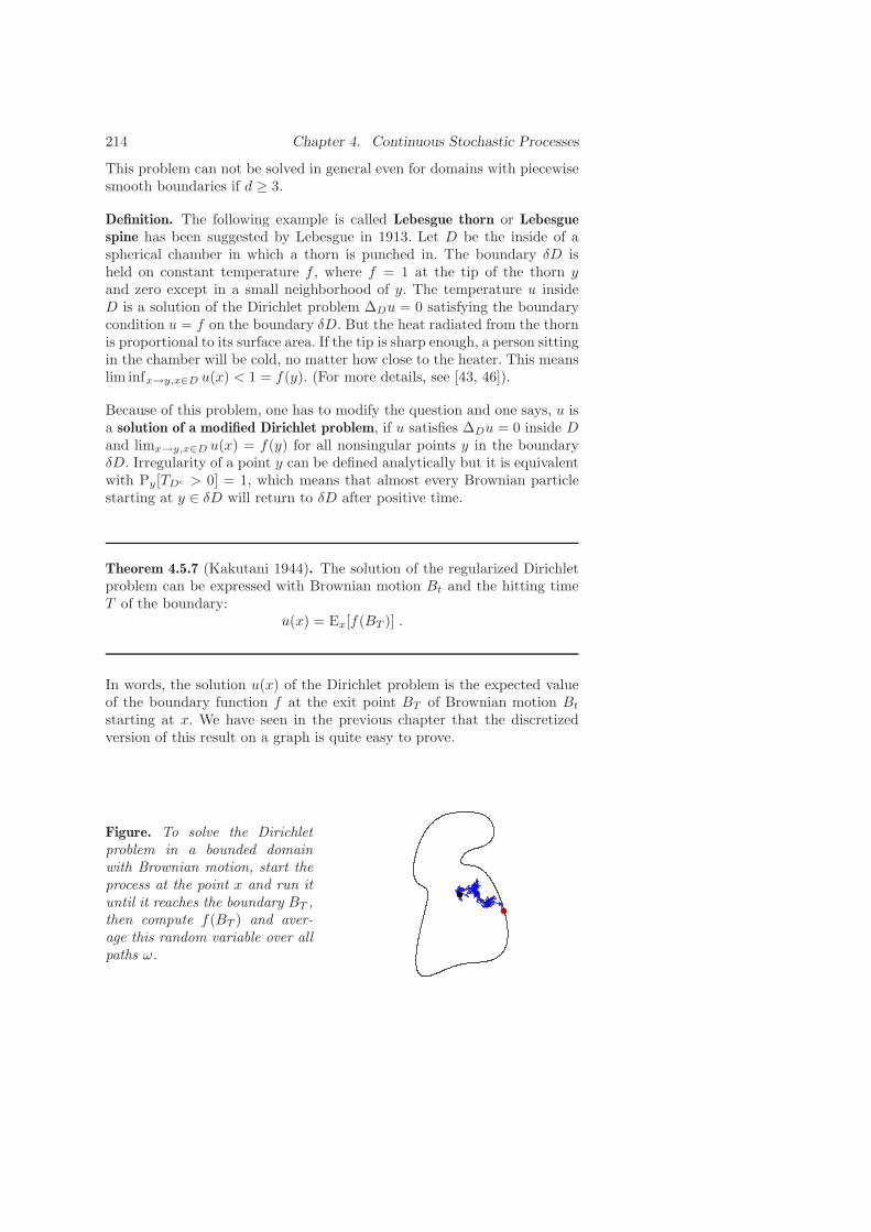
214 Chapter 4. Continuous Stochastic Processes
This problem can not be solved in general even for domains with piecewisesmooth boundaries if d ≥ 3.
Definition. The following example is called Lebesgue thorn or Lebesguespine has been suggested by Lebesgue in 1913. Let D be the inside of aspherical chamber in which a thorn is punched in. The boundary δD isheld on constant temperature f , where f = 1 at the tip of the thorn yand zero except in a small neighborhood of y. The temperature u insideD is a solution of the Dirichlet problem ∆Du = 0 satisfying the boundarycondition u = f on the boundary δD. But the heat radiated from the thornis proportional to its surface area. If the tip is sharp enough, a person sittingin the chamber will be cold, no matter how close to the heater. This meanslim infx→y,x∈D u(x) < 1 = f(y). (For more details, see [43, 46]).
Because of this problem, one has to modify the question and one says, u isa solution of a modified Dirichlet problem, if u satisfies ∆Du = 0 inside Dand limx→y,x∈D u(x) = f(y) for all nonsingular points y in the boundaryδD. Irregularity of a point y can be defined analytically but it is equivalentwith Py[TDc > 0] = 1, which means that almost every Brownian particlestarting at y ∈ δD will return to δD after positive time.
Theorem 4.5.7 (Kakutani 1944). The solution of the regularized Dirichletproblem can be expressed with Brownian motion Bt and the hitting timeT of the boundary:
u(x) = Ex[f(BT )] .
In words, the solution u(x) of the Dirichlet problem is the expected valueof the boundary function f at the exit point BT of Brownian motion Btstarting at x. We have seen in the previous chapter that the discretizedversion of this result on a graph is quite easy to prove.
Figure. To solve the Dirichletproblem in a bounded domainwith Brownian motion, start theprocess at the point x and run ituntil it reaches the boundary BT ,then compute f(BT ) and aver-age this random variable over allpaths ω.

4.6. Continuous time martingales 215
Remark. Ikeda has discovered that there exists also a probabilistic methodfor solving the classical von Neumann problem in the case d = 2. For moreinformation about this, one can consult [43, 79]. The process for the vonNeumann problem is not the process of killed Brownian motion, but theprocess of reflected Brownian motion.
Remark. Given the Dirichlet Laplacian ∆ of a bounded domain D. Onecan compute the heat flow e−t∆u by the following formula
(e−t∆u)(x) = Ex[u(Bt); t < T ] ,
where T is the hitting time of δD for Brownian motion Bt starting at x.
Remark. Let K be a compact subset of a Green domain D. The hittingprobability
p(x) = Px[TK < TδD]
is the equilibrium potential of K relative to D. We give a definition of theequilibrium potential later. Physically, the equilibrium potential is obtainedby measuring the electrostatic potential, if one is grounding the conductingboundary and charging the conducting set B with a unit amount of charge.
4.6 Continuous time martingales
Definition. Given a filtration At of the probability space (Ω,A,P). A real-valued process Xt ∈ L1 which is At adapted is called a submartingale, ifE[Xt|As] ≥ Xs, it is called a supermartingale if −X is a submartingaleand a martingale, if it is both a super and sub-martingale. If additionallyXt ∈ Lp for all t, we speak of Lp super or sub-martingales.
We have seen martingales for discrete time already in the last chapter.Brownian motion gives examples with continuous time.
Proposition 4.6.1. Let Bt be standard Brownian motion. Then Bt, B2t − t
and eαBt−α2t/2 are martingales.
Proof. Bt −Bs is independent of Bs. Therefore
E[Bt | As] −Bs = E[Bt −Bs|As] = E[Bt − Bs] = 0 .
Since by the ”extracting knowledge” property
E[BtBs | As] = Bs · E[Bt | As] = 0 ,
we get
E[B2t − t | As] − (B2
s − s) = E[B2t −B2
s | As] − (t− s)
= E[(Bt −Bs)2 | As] − (t− s) = 0 .

216 Chapter 4. Continuous Stochastic Processes
Since Brownian motion begins at any time s new, we have
E[eα(Bt−Bs)|As] = E[eαBt−s ] = eα2(t−s)/2
from whichE[eαBt |As]e
−α2t/2 = E[eαBs ]e−α2s/2
follows.
As in the discrete case, we remark:
Proposition 4.6.2. If Xt is a Lp-martingale, then |Xt|p is a submartingalefor p ≥ 1.
Proof. The conditional Jensen inequality gives
E[|Xt|p|As] ≥ |E[Xt|As]|p = |Xs|p .
Example. Let Xn be a sequence of IID exponential distributed randomvariables with probability density fX(x) = e−cxc. Let Sn =
∑nk=1Xk. The
Poisson process Nt with time T = R+ = [0,∞) is defined as
Nt =
∞∑
k=1
1Sk≤t .
It is an example of a martingale which is not continuous, This processtakes values in N and measures, how many jumps are necessary to reacht. Since E[Nt] = ct, it follows that Nt − ct is a martingale with respect tothe filtration At = σ(Ns, s ≤ t). It is a right continuous process. We knowtherefore that it is progressively measurable and that for each stoppingtime T , also NT is progressively measurable. See [49] or the last chapterfor more information about Poisson processes.
Figure. The Poisson point pro-cess on the line. Nt is the num-ber of events which happen up totime t. It could model for exam-ple the number Nt of hits onto awebsite.
1 2 3 4 5 6 7 8 9 10X X X X X X X X X X
1 2 3 4 5 6 7 8 9 10 11S S S S S S S S S S S

4.7. Doob inequalities 217
Proposition 4.6.3. (Interval theorem) The Poisson process has independentincrements
Nt −Ns =∞∑
n=1
1s<Sn≤t .
Moreover, Nt is Poisson distributed with parameter tc:
P[Nt = k] =(tc)k
k!e−tc .
Proof. The proof is done by starting with a Poisson distributed process Nt.Define then
Sn(ω) = t | Nt = n,Nt−0 = n− 1 and show that Xn = Sn − Sn−1 are independent random variables withexponential distribution.
Remark. Poisson processes on the lattice Zd are also called Brownian mo-tion on the lattice and can be used to describe Feynman-Kac formulas fordiscrete Schrodinger operators. The process is defined as follows: take Xt
as above and define
Yt =∞∑
k=1
Zk1Sk≤t ,
where Zn are IID random variables taking values in m ∈ Zd||m| = 1.This means that a particle stays at a lattice site for an exponential timeand jumps then to one of the neighbors of n with equal probability. LetPn be the analog of the Wiener measure on right continuous paths on thelattice and denote with En the expectation. The Feynman-Kac formula fordiscrete Schrodinger operators H = H0 + V is
(e−itHu)(n) = e2dtEn[u(Xt)iNte−i
R
t0V (Xs) ds] .
4.7 Doob inequalities
We have already established inequalities of Doob for discrete times T = N.By a limiting argument, they hold also for right-continuous submartingales.
Theorem 4.7.1 (Doob’s submartingale inequality). Let X be a non-negativeright continuous submartingale with time T = [a, b]. For any ǫ > 0
ǫ · P[ supa≤t≤b
Xt ≥ ǫ] ≤ E[Xb; supa≤t≤b
Xt ≥ ǫ] ≤ E[Xb] .

218 Chapter 4. Continuous Stochastic Processes
Proof. Take a countable subset D of T and choose an increasing sequenceDn of finite sets such that
⋃
nDn = D. We know now that for all n
ǫ · P[ supt∈Dn
Xt ≥ ǫ] ≤ E[Xb; supt∈Dn
Xt ≥ ǫ] ≤ E[Xb] .
since E[Xt] is nondecreasing in t. Going to the limit n→ ∞ gives the claimwith T = D. Since X is right continuous, we get the claim for T = [a, b].
One often applies this inequality to the non-negative submartingale |X | ifX is a martingale.
Theorem 4.7.2 (Doob’s Lp inequality). Fix p > 1 and q satisfying p−1 +q−1 = 1. Given a non-negative right-continuous submartingale X withtime T = [a, b] which is bounded in Lp. Then X∗ = supt∈T Xt is in Lp andsatisfies
||X∗||p ≤ q · supt∈T
||Xt||p .
Proof. Take a countable subset D of T and choose an increasing sequenceDn of finite sets such that
⋃
nDn = D.We had
|| supt∈Dn
Xt|| ≤ q · supt∈Dn
||Xt||p .
Going to the limit gives
|| supt∈D
Xt|| ≤ q · supt∈D
||Xt||p .
Since D is dense and X is right continuous we can replace D by T .
The following inequality measures, how big is the probability that one-dimensional Brownian motion will leave the cone (t, x), |x| ≤ a · t.
Theorem 4.7.3 (Exponential inequality). St = sup0≤s≤tBs satisfies for anya > 0
P[St ≥ a · t] ≤ e−a2t/2 .
Proof. We have seen in proposition (4.6.1) that Mt = eαBt−α2t2 is a mar-
tingale. It is nonnegative. Since
exp(αSt −α2t
2) ≤ exp(sup
s≤tBs −
α2t
2) ≤ sup
s≤texp(Bs −
α2s
2) = sup
s≤tMs ,

4.8. Khintchine’s law of the iterated logarithm 219
we get with Doob’s submartingale inequality (4.7.1)
P[St ≥ at] ≤ P[sups≤t
Ms ≥ eαat−α2t2 ]
≤ exp(−αat+α2t
2)E[Mt] .
The result follows from E[Bt] = E[B0] = 1 and infα>0 exp(−αat + α2t2 ) =
exp(−a2t2 ).
An other corollary of Doob’s maximal inequality will also be useful.
Corollary 4.7.4. For a, b > 0,
P[ sups∈[0,1]
(Bs −αs
2) ≥ β] ≤ e−αβ .
Proof.
P[ sups∈[0,1]
(Bs −αs
2) ≥ β] ≤ P[ sup
s∈[0,1]
(Bs −αt
2) ≥ β]
= P[ sups∈[0,1]
(eαBs−α2t2 ) ≥ eβα]
= P[ sups∈[0,1]
Ms ≥ eβα]
≤ e−βα sups∈[0,1]
E[Ms] = e−βα
since E[Ms] = 1 for all s.
4.8 Khintchine’s law of the iterated logarithm
Khinchine’s law of the iterated logarithm for Brownian motion gives a pre-cise statement about how one-dimensional Brownian motion oscillates in aneighborhood of the origin. As in the law of the iterated logarithm, define
Λ(t) =√
2t log | log t| .
Theorem 4.8.1 (Law of iterated logarithm for Brownian motion).
P[lim supt→0
BtΛ(t)
= 1] = 1, P[lim inft→0
BtΛ(t)
= −1] = 1

220 Chapter 4. Continuous Stochastic Processes
Proof. The second statement follows from the first by changing Bt to −Bt.
(i) lim sups→0Bs
Λ(s) ≤ 1 almost everywhere:
Take θ, δ ∈ (0, 1) and define
αn = (1 + δ)θ−nΛ(θn), βn =Λ(θn)
2.
We have αnβn = log log(θn)(1 + δ) = log(n) log(θ). From corollary (4.7.4),we get
P[sups≤1
(Bs −αns
2) ≥ βn] ≤ e−αnβn = Kn(−1+δ) .
The Borel-Cantelli lemma assures
P[lim infn→∞
sups≤1
(Bs −αns
2) < βn] = 1
which means that for almost every ω, there is n0(ω) such that for n > n0(ω)and s ∈ [0, θn−1),
Bs(ω) ≤ αns
2+ βn ≤ αn
θn−1
2+ βn = (
(1 + δ)
2θ+
1
2)Λ(θn) .
Since Λ is increasing on a sufficiently small interval [0, a), we have forsufficiently large n and s ∈ (θn, θn−1]
Bs(ω) ≤ ((1 + δ)
2θ+
1
2)Λ(s) .
In the limit θ → 1 and δ → 0, we get the claim.
(ii) lim sups→0Bs
Λ(s) ≥ 1 almost everywhere.
For θ ∈ (0, 1), the sets
An = Bθn −Bθn+1 ≥ (1 −√θ)Λ(θn)
are independent and since Bθn −Bθn+1 is Gaussian we have
P[An] =
∫ ∞
a
e−u2/2 du√
2π>
a
a2 + 1e−a
2/2
with a = (1 −√θ)Λ(θn) ≤ Kn−α with some constants K and α < 1.
Therefore∑
n P[An] = ∞ and by the second Borel-Cantelli lemma,
Bθn ≥ (1 −√θ)Λ(θn) +Bθn+1 (4.1)
for infinitely many n. Since −B is also Brownian motion, we know from (i)that
−Bθn+1 < 2Λ(θn+1) (4.2)
for sufficiently large n. Using these two inequalities (4.1) and (4.2) andΛ(θn+1) ≤ 2
√θΛ(θn) for large enough n, we get
Bθn > (1 −√θ)Λ(θn) − 4Λ(θn+1) > Λ(θn)(1 −
√θ − 4
√θ)

4.8. Khintchine’s law of the iterated logarithm 221
for infinitely many n and therefore
lim inft→0
BtΛ(t)
≥ lim supn→∞
Bθn
Λ(θn)> 1 − 5
√θ .
The claim follows for θ → 0.
Remark. This statement shows also that Bt changes sign infinitely oftenfor t → 0 and that Brownian motion is recurrent in one dimension. Onecould show more, namely that the set Bt = 0 is a nonempty perfect setwith Hausdorff dimension 1/2 which is in particularly uncountable.
By time inversion, one gets the law of iterated logarithm near infinity:
Corollary 4.8.2.
P[lim supt→∞
BtΛ(t)
= 1] = 1, P[lim inft→∞
BtΛ(t)
= −1] = 1 .
Proof. Since Bt = tB1/t (with B0 = 0) is a Brownian motion, we have withs = 1/t
1 = lim sups→0
BsΛ(s)
= lim sups→0
sB1/s
Λ(s)
= lim supt→∞
BttΛ(1/t)
= lim supt→∞
BtΛ(t)
.
The other statement follows again by reflection.
Corollary 4.8.3. For d-dimensional Brownian motion, one has
P[lim supt→0
BtΛ(t)
= 1] = 1, P[lim inft→0
BtΛ(t)
= −1] = 1
Proof. Let e be a unit vector in Rd. Then Bt · e is a 1-dimensional Brown-ian motion since Bt was defined as the product of d orthogonal Brownianmotions. From the previous theorem, we have
P[lim supt→0
Bt · eΛ(t)
= 1] = 1 .
Since Bt · e ≤ |Bt|, we know that the lim sup is ≥ 1. This is true for allunit vectors and we can even get it simultaneously for a dense set enn∈N

222 Chapter 4. Continuous Stochastic Processes
of unit vectors in the unit sphere. Assume the lim sup is 1 + ǫ > 1. Then,there exists en such that
P[lim supt→0
Bt · enΛ(t)
≥ 1 +ǫ
2] = 1
in contradiction to the law of iterated logarithm for Brownian motion.Therefore, we have lim sup = 1. By reflection symmetry, lim inf = −1.
Remark. It follows that in d dimensions, the set of limit points of Bt/Λ(t)for t→ 0 is the entire unit ball |v| ≤ 1.
4.9 The theorem of Dynkin-Hunt
Definition. Denote by I(k, n) the interval [k−12n , k2n ). If T is a stopping time,
then T (n) denotes its discretisation
T (n)(ω) =
∞∑
k=1
1I(k,n)(T (ω))k
2n
which is again a stopping time. Define also:
AT+ = A ∈ A∞ | A ∩ T < t ∈ At, ∀t .
The next theorem tells that Brownian motion starts afresh at stoppingtimes.
Theorem 4.9.1 (Dynkin-Hunt). Let T be a stopping time for Brownianmotion, then Bt = Bt+T − BT is Brownian motion when conditioned toT <∞ and Bt is independent of AT+ when conditioned to T <∞.
Proof. Let A be the set T <∞. The theorem says that for every function
f(Bt) = g(Bt+t1 , Bt+t2 , . . . , Bt+tn)
with g ∈ C(Rn)
E[f(Bt)1A] = E[f(Bt)] · P[A]
and that for every set C ∈ AT+
E[f(Bt)1A∩C ] · P[A] = E[f(Bt)1A] · P[A ∩ C] .
This two statements are equivalent to the statement that for every C ∈ AT+
E[f(Bt) · 1A∩C ] = E[f(Bt)] · P[A ∩ C] .
4.10. Self-intersection of Brownian motion 223
Let T (n) be the discretisation of the stopping time T and An = T (n) <∞as well as An,k = T (n) = k/2n. Using A = T <∞,P[
⋃∞k=1 An,k∩C] →
P[A ∩ C] for n→ ∞, we compute
E[f(Bt)1A∩C ] = limn→∞
E[f(BT (n))1An∩C ]
= limn→∞
∞∑
k=0
E[f(Bk/2n)1An,k∩C ]
= limn→∞
∞∑
k=0
E[f(B0)] · P[An,k ∩C]
= E[f(B0)] limn→∞
P[
∞⋃
k=1
An,k ∩ C]
= E[f(B0)1A∩C ]
= E[f(B0)] · P[A ∩ C]
= E[f(Bt)] · P[A ∩ C] .
Remark. If T < ∞ almost everywhere, no conditioning is necessary andBt+T −BT is again Brownian motion.
Theorem 4.9.2 (Blumental’s zero-one law). For every set A ∈ A0+ we haveP[A] = 0 or P[A] = 1.
Proof. Take the stopping time T which is identically 0. Now B = Bt+T −Bt = B. By Dynkin-Hunt’s result, we know that B = B is independent ofBT+ = A0+ . Since every C ∈ A0+ is Bs, s > 0 measurable, we know thatA0+ is independent to itself.
Remark. This zero-one law can be used to define regular points on theboundary of a domain D ∈ Rd. Given a point y ∈ δD. We say it is regular,if Py[TδD > 0] = 0 and irregular Py[TδD > 0] = 1. This definition turnsout to be equivalent to the classical definition in potential theory: a pointy ∈ δD is irregular if and only if there exists a barrier function f : N → R
in a neighborhood N of y. A barrier function is defined as a negative sub-harmonic function on int(N ∩ D) satisfying f(x) → 0 for x → y withinD.
4.10 Self-intersection of Brownian motion
Our aim is to prove the following theorem:

224 Chapter 4. Continuous Stochastic Processes
Theorem 4.10.1 (Self intersections of random walk). For d ≤ 3, Brownianmotion has infinitely many self intersections with probability 1.
Remark. Kakutani, Dvoretsky and Erdos have shown that for d > 3, thereare no self-intersections with probability 1. It is known that for d ≤ 2, thereare infinitely many n−fold points and for d ≥ 3, there are no triple points.
Proposition 4.10.2. LetK be a compact subset of Rd and T the hitting timeof K with respect to Brownian motion starting at y. The hitting probabilityh(y) = P[y + Bs ∈ K,T ≤ s <∞] is a harmonic function on Rd \K.
Proof. Let Tδ be the hitting time of Sδ = |x − y| = δ. By the law ofiterated logarithm, we have Tδ < ∞ almost everywhere. By Dynkin-Hunt,we know that Bt = Bt+Tδ
−Bt is again Brownian motion.
If δ is small enough, then y + Bs /∈ K for t ≤ Tδ. The random variableBTδ
∈ Sδ has a uniform distribution on Sδ because Brownian motion isrotational symmetric. We have therefore
h(y) = P[y +Bs ∈ K, s ≥ Tδ]
= P[y +BTδ+ B ∈ K]
=
∫
Sδ
h(y + x) dµ(x) ,
where µ is the normalized Lebesgue measure on Sδ. This equality for smallenough δ is the definition of harmonicity.
Proposition 4.10.3. Let K be a countable union of closed balls. Thenh(K, y) → 1 for y → K.
Proof. (i) We show the claim first for one ballK = Br(z) and letR = |z−y|.By Brownian scaling Bt ∼ c · Bt/c2 . The hitting probability of K can onlybe a function f(r/R) of r/R:
h(y,K) = P[y +Bs ∈ K,T ≤ s] = P[cy +Bs/c2 ∈ cK, TK ≤ s]
= P[cy +Bs/c2 ∈ cK, TcK ≤ s/c2]
= P[cy +Bs, TcK ≤ s]
= h(cy, cK) .

4.10. Self-intersection of Brownian motion 225
We have to show therefore that f(x) → 1 as x→ 1. By translation invari-ance, we can fix y = y0 = (1, 0, . . . , 0) and change Kα, which is a ball ofradius α around (−α, 0, . . . ). We have
h(y0,Kα) = f(α/(1 + α))
and take therefore the limit α→ ∞
limx→1
f(x) = limα→∞
h(y0,Kα) = h(y0,⋃
Kα)
= E[infs≥0
(Bs)1 < −1] = 1
because of the law of iterated logarithm.(ii) Given yn → y0 ∈ K. Then y0 ∈ K0 for some ball K0.
lim infn→∞
h(yn,K) ≥ limn→∞
h(yn,K0) = 1
by (i).
Definition. Let µ be a probability measure on R3. Define the potentialtheoretical energy of µ as
I(µ) =
∫
R3
∫
R3
|x− y|−1 dµ(x) dµ(y) .
Given a compact set K ⊂ R3, the capacity of K is defined as
( infµ∈M(K)
I(µ))−1 ,
where M(K) is the set of probability measures on K. A measure on Kminimizing the energy is called an equilibrium measure.
Remark. This definitions can be done in any dimension. In the case d =2, one replaces |x − y|−1 by log |x − y|−1. In the case d ≥ 3, one takes|x− y|−(d−2). The capacity is for d = 2 defined as exp(− infµ I(µ)) and ford ≥ 3 as (infµ I(µ))−(d−2).
Definition. We say a measure µn on Rd converges weakly to µ, if for all con-tinuous functions f ,
∫
f dµn →∫
f dµ. The set of all probability measureson a compact subset E of Rd is known to be compact.
The next proposition is part of Frostman’s fundamental theorem of poten-tial theory. For detailed proofs, we refer to [39, 80].
Proposition 4.10.4. For every compact set K ⊂ Rd, there exists an equilib-rium measure µ on K and the equilibrium potential
∫
|x − y|−(d−2) dµ(y)rsp.
∫
log(|x − y|−1) dµ(y) takes the value C(K)−1 on the support K∗ ofµ.
226 Chapter 4. Continuous Stochastic Processes
Proof. (i) (Lower semicontinuity of energy) If µn converges to µ, then
lim infn→∞
I(µn) ≥ I(µ) .
(ii) (Existence of equilibrium measure) The existence of an equilibrium mea-sure µ follows from the compactness of the set of probability measures onK and the lower semicontinuity of the energy since a lower semi-continuousfunction takes a minimum on a compact space. Take a sequence µn suchthat
I(µn) → infµ∈M(K)
I(µ) .
Then µn has an accumulation point µ and I(µ) ≤ infµ∈M(K) I(µ).
(iii) (Value of capacity) If the potential φ(x) belonging to µ is constant onK, then it must take the value C(K)−1 since
∫
φ(x) dµ(x) = I(µ) .
(iv) (Constancy of capacity) Assume the potential is not constant C(K)−1
on K∗. By constructing a new measure on K∗ one shows then that one canstrictly decrease the energy. This is physically evident if we think of φ asthe potential of a charge distribution µ on the set K.
Corollary 4.10.5. Let µ be the equilibrium distribution on K. Then
h(y,K) = φµ · C(K)
and therefore h(y,K) ≥ C(K) · infx∈K |x− y|−1.
Proof. Assume first K is a countable union of balls. According to proposi-tion (4.10.2) and proposition (4.10.3), both functions h and φµ · C(K) areharmonic, zero at ∞ and equal to 1 on δ(K). They must therefore be equal.For a general compact set K, let yn be a dense set in K and let Kǫ =⋃
nBǫ(yn). One can pass to the limit ǫ→ 0. Both h(y,Kǫ) → h(y,K) andinfx∈Kǫ |x − y|−1 → infx∈K |x − y|−1 are clear. The statement C(Kǫ) →C(K) follows from the upper semicontinuity of the capacity: if Gn is a se-quence of open sets with ∩Gn = E, then C(Gn) → C(E).The upper semicontinuity of the capacity follows from the lower semicon-tinuity of the energy.

4.10. Self-intersection of Brownian motion 227
Proposition 4.10.6. Assume, the dimension d = 3. For any interval J =[a, b], the set
BJ(ω) = Bt(ω) | t ∈ [a, b]has positive capacity for almost all ω.
Proof. We have to find a probability measure µ(ω) on BI(ω) such that itsenergy I(µ(ω)) is finite almost everywhere. Define such a measure by
dµ(A) = | s ∈ [a, b] | Bs ∈ A(b− a)
| .
Then
I(µ) =
∫ ∫
|x− y|−1 dµ(x)dµ(y) =
∫ b
a
∫ b
a
(b− a)−1|Bs −Bt|−1 dsdt .
To see the claim we have to show that this is finite almost everywhere, weintegrate over Ω which is by Fubini
E[I(µ)] =
∫ b
a
∫ b
a
(b− a)−1E[|Bs −Bt|−1] dsdt
which is finite since Bs − Bt has the same distribution as√s− tB1 by
Brownian scaling and since E[|B1|−1] =∫
|x|−1e−|x|2/2 dx < ∞ in dimen-
sion d ≥ 2 and∫ b
a
∫ b
a
√s− t ds dt <∞.
Now we prove the theorem
Proof. We have only to show that in the case d = 3. Because Brownianmotion projected to the plane is two dimensional Brownian and to the lineis one dimensional Brownian motion, the result in smaller dimensions fol-low.
(i) α = P[⋃
t∈[0,1],s≥2Bt = Bs] > 0.
Proof. Let K be the set⋃
t∈[0,1]Bt. We know that it has positive capacity
almost everywhere and that therefore h(Bs,K) > 0 almost everywhere.But h(Bs,K) = α since Bs+2 − Bs is Brownian motion independent ofBs, 0 ≤ s ≤ 1.
(ii) αT = P[⋃
t∈[0,1],2≤T Bt = Bs] > 0 for some T > 0. Proof. Clear sinceαT → α for T → ∞.(iii) Proof of the claim. Define the random variables Xn = 1Cn with
Cn = ω | Bt = Bs, for some t ∈ [nT, nT + 1], s ∈ [nT + 2, (n+ 1)T ] .
They are independent and by the strong law of large numbers∑
nXn = ∞almost everywhere.

228 Chapter 4. Continuous Stochastic Processes
Corollary 4.10.7. Any point Bs(ω) is an accumulation point of self-crossingsof Bt(ω)t≥0.
Proof. Again, we have only to treat the three dimensional case. Let T > 0be such that
αT = P[⋃
t∈[0,1],2≤TBt = Bs] > 0
in the proof of the theorem. By scaling,
P[Bt = Bs | t ∈ [0, β], s ∈ [2β, Tβ] ]
is independent of β. We have thus self-intersections of the random walk inany interval [0, b] and by translation in any interval [a, b].
4.11 Recurrence of Brownian motion
We show in this section that like its discrete brother, the random walk,Brownian motion is transient in dimensions d ≥ 3 and recurrent in dimen-sions d ≤ 2.
Lemma 4.11.1. Let T be a finite stopping time and RT (ω) be a rotation inRd which turns BT (ω) onto the first coordinate axis
RT (ω)BT (ω) = (|BT (ω)|, 0, . . . 0) .
Then Bt = RT (Bt+T −BT ) is again Brownian motion.
Proof. By the Dynkin-Hunt theorem, Bt = Bt+T −BT is Brownian motionand independent of AT . By checking the definitions of Brownian motion,it follows that if B is Brownian motion, also R(x)Bt is Brownian motion,if R(x) is a random rotation on Rd independent of Bt. Since RT is AT
measurable and Bt is independent of AT , the claim follows.
Lemma 4.11.2. Let Kr be the ball of radius r centered at 0 ∈ Rd withd ≥ 3. We have for y /∈ Kr
h(y,Kr) = (r/|y|)d−2 .

4.11. Recurrence of Brownian motion 229
Proof. Both h(y,Kr) and (r/|y|)d−2 are harmonic functions which are 1 atδKr and zero at infinity. They are the same.
Theorem 4.11.3 (Escape of Brownian motion in three dimensions). Ford ≥ 3, we have limt→∞ |Bt| = ∞ almost surely.
Proof. Define a sequence of stopping times Tn by
Tn = infs > 0 | |Bs| = 2n ,which is finite almost everywhere because of the law of iterated logarithm.We know from the lemma (4.11.1) that
Bt = RTn(Bt+Tn −BTn)
is a copy of Brownian motion. Clearly also |BTn | = 2n.We have Bs ∈ Kr(0) = |x| < r for some s > Tn if and only if Bt ∈(2n, 0 . . . , 0) +Kr(0) for some t > 0.Therefore using the previous lemma
P[Bs ∈ Kr(0); s > Tn] = P[Bt ∈ (2n, 0 . . . , 0) +Kr(0); t > 0] = (r
2n)d−2
which implies in the case r2−n < 1 by the Borel-Cantelli lemma that foralmost all ω, Bs(ω) ≥ r for s > Tn. Since Tn is finite almost everywhere,we get lim infs |Bs| ≥ r. Since r is arbitrary, the claim follows.
Brownian motion is recurrent in dimensions d ≤ 2. In the case d = 1, thisfollows readily from the law of iterated logarithm. First a lemma
Lemma 4.11.4. In dimensions d = 2, almost every path of Brownian motionhits a ball Kr if r > 0: one has h(y,K) = 1.
Proof. We know that h(y) = h(y,K) is harmonic and equal to 1 on δK. Itis also rotational invariant and therefore h(y) = a+b log |y|. Since h ∈ [0, 1]we have h(y) = a and so a = 1.
Theorem 4.11.5 (Recurrence of Brownian motion in 1 or 2 dimensions). Letd ≤ 2 and S be an open nonempty set in Rd. Then the Lebesgue measureof t | Bt ∈ S is infinite.

230 Chapter 4. Continuous Stochastic Processes
Proof. It suffices to take S = Kr(x0), a ball of radius r around x0. Sinceby the previous lemma, Brownian motion hits every ball almost surely, wecan assume that x0 = 0 and by scaling that r = 1.Define inductively a sequence of hitting or leaving times Tn, Sn of theannulus 1/2 < |x| < 2, where T1 = inft | |Bt| = 2 and
Sn = inft > Tn | |Bt| = 1/2Tn = inft > Sn−1 | |Bt| = 2 .
These are finite stopping times. The Dynkin-Hunt theorem shows that Sn−Tn and Tn − Sn−1 are two mutually independent families of IID randomvariables. The Lebesgue measures Yn = |In| of the time intervals
In = t | |Bt| ≤ 1, Tn ≤ t ≤ Tn+1 ,
are independent random variables. Therefore, also Xn = min(1, Yn) areindependent bounded IID random variables. By the law of large numbers,∑
nXn = ∞ which implies∑
n Yn = ∞ and the claim follows from
|t ∈ [0,∞) | |Bt| ≤ 1 | ≥∑
n
Tn .
Remark. Brownian motion in Rd can be defined as a diffusion on Rd withgenerator ∆/2, where ∆ is the Laplacian on Rd. A generalization of Brow-nian motion to manifolds can be done using the diffusion processes withrespect to the Laplace-Beltrami operator. Like this, one can define Brown-ian motion on the torus or on the sphere for example. See [57].
4.12 Feynman-Kac formula
In quantum mechanics, the Schrodinger equation i~u = Hu defines theevolution of the wave function u(t) = e−itH/~u(0) in a Hilbert space H. TheoperatorH is the Hamiltonian of the system. We assume, it is a Schrodingeroperator H = H0 + V , where H0 = −∆/2 is the Hamiltonian of a freeparticle and V : Rd → R is the potential. The free operator H0 already isnot defined on the whole Hilbert space H = L2(Rd) and one restricts H toa vector space D(H) called domain containing the in H dense set C∞
0 (Rd)of all smooth functions which are zero at infinity. Define
D(A∗) = u ∈ H | v 7→ (Av, u) is a bounded linear functional on D(A).
If u ∈ D(A∗), then there exists a unique function w = A∗u ∈ H such that(Av, u) = (v, w) for all u ∈ D(A). This defines the adjoint A∗ of A withdomain D(A∗).
Definition. A linear operator A : D(A) ⊂ H → H is called symmetric if(Au, v) = (u,Av) for all u, v ∈ D(A) and self-adjoint, if it is symmetric andD(A) = D(A∗).

4.12. Feynman-Kac formula 231
Definition. A sequence of bounded linear operators An converges stronglyto A, if Anu→ Au for all u ∈ H. One writes A = s− limn→∞ An.
Define eA = 1 + A + A2/2! + A3/3! + · · · . We will use the fact that aself-adjoint operator defines a one parameter family of unitary operatorst 7→ eitA which is strongly continuous. Moreover, eitA leaves the domainD(A) of A invariant. For more details, see [81, 7].
Theorem 4.12.1 (Trotter product formula). Given self-adjoint operatorsA,B defined on D(A), D(B) ⊂ H. Assume A + B is self-adjoint on D =D(A) ∩D(B), then
eit(A+B) = s− limn→∞
(eitA/neitB/n)n .
If A,B are bounded from below, then
e−t(A+B) = s− limn→∞
(e−tA/ne−tB/n)n .
Proof. Define
St = eit(A+B), Vt = eitA,Wt = eitB, Ut = VtWt
and vt = Stv for v ∈ D. Because A+B is self-adjoint on D, one has vt ∈ D.Use a telescopic sum to estimate
||(St − Unt/n)v|| = ||n−1∑
j=0
U jt/n(St/n − Ut/n)Sn−j−1t/n v||
≤ n sup0≤s≤t
||(St/n − Ut/n)vs|| .
We have to show that this goes to zero for n → ∞. Given u ∈ D =D(A) ∩D(B),
lims→0
Ss − 1
su = i(A+B)u = lim
s→0
Us − 1
su
so that for each u ∈ D
limn→∞
n · ||(St/n − Ut/n)u|| = 0 . (4.3)
The linear space D with norm |||u||| = ||(A + B)u|| + ||u|| is a Banachspace since A + B is self-adjoint on D and therefore closed. We have abounded family n(St/n − Ut/n)n∈N of bounded operators from D to H.The principle of uniform boundedness states that
||n(St/n − Ut/n)u|| ≤ C · |||u||| .
232 Chapter 4. Continuous Stochastic Processes
An ǫ/3 argument shows that the limit (4.3) exists uniformly on compactsubsets of D and especially on vss∈[0,t] ⊂ D and so n sup0≤s≤t ||(St/n −Ut/n)vs|| = 0. The second statement is proved in exactly the same way.
Remark. Trotter’s product formula generalizes the Lie product formula
limn→∞
(exp(A
n) exp(
B
n))n = exp(A+B)
for finite dimensional matrices A,B, which is a special case.
Corollary 4.12.2. (Feynman 1948) Assume H = H0 + V is self-adjoint onD(H). Then
e−itHu(x0) = limn→∞
(2πit
n)−d/2
∫
(Rd)n
eiSn(x0,x1,x2,...,xn,t)u(xn) dx1 . . . dxn
where
Sn(x0, x1, . . . , xn, t) =t
n
n∑
i=1
1
2(|xi − xi−1|
t/n)2 − V (xi) .
Proof. (Nelson) From u = −iH0u, we get by Fourier transform ˙u = i |k|2
2 u
which gives ut(k) = exp(i |k|2|
2 t)u0(k) and by inverse Fourier transform
e−itH0u(x) = ut(x) = (2πit)−d/2∫
Rd
ei|x−y|2
2t u(y) dy .
The Trotter product formula
e−it(H0+V ) = s− limn→∞
(eitH0/neitV/n)n
gives now the claim.
Remark. We did not specify the set of potentials, for which H0 +V can bemade self-adjoint. For example, V ∈ C∞
0 (Rν) is enough or V ∈ L2(R3) ∩L∞(R3) in three dimensions.
We have seen in the above proof that e−itH0 has the integral kernel Pt(x, y) =
(2πit)−d/2ei|x−y|2
2t . The same Fourier calculation shows that e−tH0 has theintegral kernel
Pt(x, y) = (2πt)−d/2e−|x−y|2
2t ,
where gt is the density of a Gaussian random variable with variance t.Note that even if u ∈ L2(Rd) is only defined almost everywhere, the func-tion ut(x) = e−tH0u(x) =
∫
Pt(x − y)u(y)dy is continuous and defined

4.12. Feynman-Kac formula 233
everywhere.
Lemma 4.12.3. Given f1, . . . , fn ∈ L∞(Rd)∩L2(Rd) and 0 < s1 < · · · < sn.Then
(e−t1H0f1 · · · e−tnH0fn)(0) =
∫
f1(Bs1) · · · fn(Bsn) dB,
where t1 = s1, ti = si − si−1, i ≥ 2 and the fi on the left hand side areunderstood as multiplication operators on L2(Rd).
Proof. Since Bs1 , Bs2 − Bs1 , . . . Bsn − Bsn−1 are mutually independentGaussian random variables of variance t1, t2, . . . , tn, their joint distribu-tion is
Pt1(0, y1)Pt2(0, y2) . . . Ptn(0, yn) dy
which is after a change of variables y1 = x1, yi = xi − xi−1
Pt1(0, x1)Pt2(x1, x2) . . . Ptn(xn−1, xn) dx .
Therefore,
∫
f1(Bs1) · · · fn(Bsn) dB
∫
(Rd)n
Pt1(0, y1)Pt2(0, y2) . . . Ptn(0, yn)f1(y1) . . . fn(yn) dy
=
∫
(Rd)n
Pt1(0, x1)Pt2(x1, x2) . . . Ptn(xn−1, xn)f1(x1) . . . fn(xn) dx
= (e−t1H0f1 · · · e−tnH0fn)(0) .
Denote by dB the Wiener measure on C([0,∞),Rd) and with dx theLebesgue measure on Rd. We define also an extended Wiener measuredW = dx× dB on C([0,∞),Rd) on all paths s 7→Ws = x+Bs starting atx ∈ Rd.
Corollary 4.12.4. Given f0, f1, . . . , fn ∈ L∞(Rd) ∩ L2(Rd) and 0 < s1 <· · · < sn. Then
∫
f0(Ws0 ) · · · fn(Wsn) dW = (f0, e−t1H0f1 · · · e−tnH0fn) .

234 Chapter 4. Continuous Stochastic Processes
Proof. (i) Case s0 = 0. From the above lemma, we have after the dBintegration that
∫
f0(Ws0) · · · fn(Wsn) dW =
∫
Rd
f0(x)e−t1H0f1(x) · · · e−tnH0fn(x) dx
= (f0, e−t1H0f1 · · · e−tnH0fn) .
(ii) In the case s0 > 0 we have from (i) and the dominated convergencetheorem
∫
f0(Ws0 ) · · · fn(Wsn) dW
= limR→∞
∫
Rd
1|x|<R(W0)
f0(Ws0 ) · · · fn(Wsn) dW
= limR→∞
(f0e−s0H01|x|<R, e
−t1H0f1 · · · e−tnH0fn(x))
= (f0, e−t1H0f1 · · · e−tnH0fn) .
We prove now the Feynman-Kac formula for Schrodinger operators of theform H = H0 +V with V ∈ C∞
0 (Rd). Because V is continuous, the integral∫ t
0 V (Ws(ω)) ds can be taken for each ω as a limit of Riemann sums and∫ t
0 V (Ws) ds certainly is a random variable.
Theorem 4.12.5 (Feynman-Kac formula). Given H = H0 + V with V ∈C∞
0 (Rd), then
(f, e−tHg) =
∫
f(W0)g(Wt)e−
R
t0V (Ws)) ds dW .
Proof. (Nelson) By the Trotter product formula
(f, e−tHg) = limn→∞
(f, (e−tH0/ne−tV/n)ng)
so that by corollary (4.12.4)
(f, e−tHg) = limn→∞
∫
f(W0)g(Wt) exp(− t
n
n−1∑
j=0
V (Wtj/n)) dW (4.4)
and since s 7→Ws is continuous, we have almost everywhere
t
n
n−1∑
j=0
V (Wtj/n) →∫ t
0
V (Ws) ds .

4.13. The quantum mechanical oscillator 235
The integrand on the right hand side of (4.4) is dominated by
|f(W0)| · |g(Wt)| · et||V ||∞
which is in L1(dW ) because again by corollary (4.12.4),∫
|f(W0)| · |g(Wt)| dW = (|f |, e−tH0 |g|) <∞ .
The dominated convergence theorem leads us now to the claim.
Remark. The formula can be extended to larger classes of potentials likepotentials V which are locally in L1. The selfadjointness, which needed inTrotter’s product formula, is assured if V ∈ L2 ∩ Lp with p > d/2. AlsoTrotter’s product formula allows further generalizations [93, 31].
Why is the Feynman-Kac formula useful?
• One can use Brownian motion to study Schrodinger semigroups. It al-lows for example to give an easy proof of the ArcSin-law for Brownianmotion.
• One can treat operators with magnetic fields in a unified way.
• Functional integration is a way of quantization which generalizes tomore situations.
• It is useful to study ground states and ground state energies underperturbations.
• One can study the classical limit ~ → 0.
4.13 The quantum mechanical oscillator
The one-dimensional Schrodinger operator
H = H0 + U = −1
2
d2
dx2+
1
2x2 − 1
2
is the Hamiltonian of the quantum mechanical oscillator. It is a quantummechanical system which can be solved explicitly like its classical analog,which has the Hamiltonian H(x, p) = 1
2p2 + 1
2x2 − 1
2 .
One can writeH = AA∗ − 1 = A∗A ,
with
A∗ =1√2(x − d
dx), A =
1√2(x+
d
dx) .
The first order operator A∗ is also called particle creation operator and A,the particle annihilation operator. The space C∞
0 of smooth functions ofcompact support is dense in L2(R). Because for all u, v ∈ C∞
0 (R)
(Au, v) = (u,A∗v)

236 Chapter 4. Continuous Stochastic Processes
the two operators are adjoint to each other. The vector
Ω0 =1
π1/4e−x
2/2
is a unit vector because Ω20 is the density of a N(0, 1/
√2) distributed ran-
dom variable. Because AΩ0 = 0, it is an eigenvector of H = A∗A witheigenvalue 1/2. It is called the ground state or vacuum state describing thesystem with no particle. Define inductively the n-particle states
Ωn =1√nA∗Ωn−1
by creating an additional particle from the (n− 1)-particle state Ωn−1 .
Figure. The first Hermit func-tions Ωn. They are unit vectorsin L2(R) defined by
Ωn(x) =Hn(x)ω0(x)√
2nn!,
where Hn(x) are Hermite poly-nomials, H0(x) = 1, H1(x) =2x,H2(x) = 4x2 − 2, H3(x) =8x3 − 12x, . . . .
Theorem 4.13.1 (Quantum mechanical oscillator). The following propertieshold:a) The functions are orthonormal (Ωn,Ωm) = δn,m.b) AΩn =
√nΩn−1, A
∗Ωn =√n+ 1Ωn+1.
c) (n− 12 ) are the eigenvalues of H
H = (A∗A− 1
2)Ωn = (n− 1
2)Ωn
.d) The functions Ωn form a basis in L2(R).
Proof. Denote by [A,B] = AB − BA the commutator of two operators Aand B. We check first by induction the formula
[A, (A∗)n] = n · (A∗)n−1 .

4.13. The quantum mechanical oscillator 237
For n = 1, this means [A,A∗] = 1. The induction step is
[A, (A∗)n] = [A, (A∗)n−1]A∗ + (A∗)n−1[A,A∗]
= (n− 1)(A∗)n−1 + (A∗)n−1 = n(A∗)n−1 .
a) Also
((A∗)nΩ0, (A∗)mΩ0) = n!δmn .
can be proven by induction. For n = 0 it follows from the fact that Ω0 isnormalized. The induction step uses [A, (A∗)n] = n · (A∗)n−1 and AΩ0 = 0:
((A∗)nΩ0, (A∗)mΩ0) = (A(A∗)nΩ0(A
∗)m−1Ω0)
= ([A, (A∗)n]Ω0(A∗)m−1Ω0)
= n((A∗)n−1Ω0, (A∗)m−1Ω0) .
If n < m, then we get from this 0 after n steps, while in the case n = m,we obtain ((A∗)nΩ0, (A
∗)nΩ0) = n · ((A∗)n−1Ω0, (A∗)n−1Ω0), which is by
induction n(n− 1)!δn−1,n−1 = n!.
b) A∗Ωn =√n+ 1 · Ωn+1 is the definition of Ωn.
AΩn =1√n!A(A∗)nΩ0 =
1√n!nΩ0 =
√nΩn−1 .
c) This follows from b) and the definition Ωn = 1√nA∗Ωn−1.
d) Part a) shows that Ωn∞n=0 it is an orthonormal set in L2(R). In orderto show that they span L2(R), we have to verify that they span the denseset
S = f ∈ C∞0 (R) | xmf (n)(x) → 0, |x| → ∞, ∀m,n ∈ N
called the Schwarz space. The reason is that by the Hahn-Banach theorem,a function f must be zero in L2(R) if it is orthogonal to a dense set. So,lets assume (f,Ωn) = 0 for all n. Because A∗ +A =
√2x
0 =√n!2n (f,Ωn) = (f, (A∗)nΩ0) = (f, (A∗ +A)nΩ0) = 2n/2 (f, xnΩ0)
we have
(fΩ0)ˆ(k) =
∫ ∞
−∞f(x)Ω0(x)e
ikx dx
= (f,Ω0eikx) = (f,
∑
n≥0
(ikx)n
n!Ω0)
=∑
n≥0
(ik)n
n!(f, xnΩ0) = 0 .
and so fΩ0 = 0. Since Ω0(x) is positive for all x, we must have f = 0. Thisfinishes the proof that we have a complete basis.

238 Chapter 4. Continuous Stochastic Processes
Remark. This gives a complete solution to the quantum mechanical har-monic oscillator. With the eigenvalues λn = n−1/2∞n=0 and the completeset of eigenvectors Ωn one can solve the Schrodinger equation
i~d
dtu = Hu
by writing the function u(x) =∑∞n=0 unΩn(x) as a sum of eigenfuctions,
where un = (u,Ωn). The solution of the Schrodinger equation is
u(t, x) =∞∑
n=0
unei~(n−1/2)tΩn(x) .
Remark. The formalism of particle creation and annihilation operatorscan be extended to some potentials of the form U(x) = q2(x) − q′(x) theoperator H = −D2/2 + U/2 can then be written as H = A∗A, where
A∗ =1√2(q(x) − d
dx), A =
1√2(q(x) +
d
dx) .
The oscillator is the special case q(x) = x. See [12]. The Backlund transfor-mation H = A∗A 7→ H = AA∗ is in the case of the harmonic oscillator themap H 7→ H + 1 has the effect that it replaces U with U = U − ∂2
x log Ω0,where Ω0 is the lowest eigenvalue. The new operator H has the same spec-trum as H except that the lowest eigenvalue is removed. This procedurecan be reversed and to create ”soliton potentials” out of the vacuum. Itis also natural to use the language of super-symmetry as introduced byWitten: take two copies Hf ⊕Hb of the Hilbert space where ”f” stands forFermion and ”b” for Boson. With
Q =
[
0 A∗
A 0
]
, P =
[
1 00 −1
]
,
one can write H ⊕ H = Q2, P 2 = 1, QP + PQ = 0 and one says (H,P,Q)has super-symmetry. The operator Q is also called a Dirac operator. Asuper-symmetric system has the property that nonzero eigenvalues havethe same number of bosonic and fermionic eigenstates. This implies that Hhas the same spectrum as H except that lowest eigenvalue can disappear.
Remark. In quantum field theory, there exists a process called canonicalquantization, where a quantum mechanical system is extended to a quan-tum field. Particle annihilation and creation operators play an importantrole.
4.14 Feynman-Kac for the oscillator
We want to treat perturbations L = L0 + V of the harmonic oscillatorL0 with an similar Feynman-Kac formula. The calculation of the integral

4.14. Feynman-Kac for the oscillator 239
kernel pt(x, y) of e−tL0 satisfying
(e−tL0f)(x) =
∫
R
pt(x, y)f(y) dy
is slightly more involved than in the case of the free Laplacian. Let Ω0 bethe ground state of L0 as in the last section.
Lemma 4.14.1. Given f0, f1, . . . , fn ∈ L∞(R) and −∞ < s0 < s1 < · · · <sn <∞. Then
(Ω0, f0e−t1L0f1 · · · e−tnL0fnΩ0) =
∫
f0(Qs0) · · · fn(Qsn) dQ ,
where t0 = s0, ti = si − si−1, i ≥ 1.
Proof. The Trotter product formula for L0 = H0 + U gives
(Ω0, f0e−t1L0f1 · · · e−tnL0fnΩ0)
= limm=(m1,...,mn),mi→∞
(Ω0, f0(e−t1H0/m1e−t1U/m1)m1f1 · · · e−tnH0fnΩ0)
=
∫
f0(x0) · · · fn(xn) dGm(x, y)
and Gm is a measure. Since e−tH0 has a Gaussian kernel and e−tU is amultiple of a Gaussian density and integrals are Gaussian, the measure dGmis Gaussian converging to a Gaussian measure dG. Since L0(xΩ0) = xΩ0
and (xΩ0, xΩ0) = 1/2 we have
∫
xixj dG = (xΩ0, e−(sj−si)L0xΩ0) =
1
2e−(sj−si)
which shows that dG is the joint probability distribution of Qs0 , . . . Qsn .The claim follows.
Theorem 4.14.2 (Mehler formula). The kernel pt(x, y) of L0 is given by theMehler formula
pt(x, y) =1√πσ2
exp
(
− (x2 + y2)(1 + e−2t) − 4xye−t
2σ2
)
.
with σ2 = (1 − e−2t).

240 Chapter 4. Continuous Stochastic Processes
Proof. We have
(f, e−tL0g) =
∫
f(y)Ω−10 (y)g(x)Ω−1
0 (x) dG(x, y) =
∫
f(y)pt(x, y) dy
with the Gaussian measure dG having covariance
A =1
2
[
1 e−t
e−t 1
]
.
We get Mehler’s formula by inverting this matrix and using that the densityis
(2π) det(A)−1/2e−((x,y),A(x,y)) .
Definition. Let dQ be the Wiener measure on C(R) belonging to the os-cillator process Qt.
Theorem 4.14.3 (Feynman-Kac for oscillator process). Given L = L0 + Vwith V ∈ C∞
0 (R), then
(fΩ0, e−iLgΩ0) =
∫
f(Q0)g(Qt)e−
R t0V (Qs)) ds dQ
for all f, g ∈ L2(R,Ω20dx).
Proof. By the Trotter product formula
(fΩ0, e−iLgΩ0) = lim
n→∞(fΩ0, (e
−tL0/ne−tV/n)ngΩ0)
so that
(fΩ0, e−iLgΩ0) = lim
n→∞
∫
f(Q0)g(Qt) exp(− t
n
n−1∑
j=0
V (Qtj/n)) dQ . (4.5)
and since Q is continuous, we have almost everywhere
t
n
n−1∑
j=0
V (Qtj/n) →∫ t
0
V (Qs) ds .
The integrand on the right hand side of (4.5) is dominated by
|f(Q0)||g(Qt)|et||V ||∞
which is in L1(dQ) since∫
|f(Q0)||g(Qt)| dQ = (Ω0|f |, e−tL0Ω0|g|) <∞ .
The dominated convergence theorem gives the claim.

4.15. Neighborhood of Brownian motion 241
4.15 Neighborhood of Brownian motion
The Feynman-Kac formula can be used to understand the Dirichlet Lapla-cian of a domain D ⊂ Rd. For more details, see [93].
Example. LetD be an open set in Rd such that the Lebesgue measure |D| isfinite and the Lebesgue measure of the boundary |δD| is zero. Denote byHD
the Dirichlet Laplacian −∆/2. Denote by kD(E) the number of eigenvaluesof HD below E. This function is also called the integrated density of states.Denote with Kd the unit ball in Rd and with |Kd| = Vol(Kd) = πd/2Γ(d2 +1)−1 its volume. Weyl’s formula describes the asymptotic behavior of kD(E)for large E:
limE→∞
kD(E)
Ed/2=
|Kd| · |D|2d/2πd
.
It shows that one can read off the volume of D from the spectrum of theLaplacian.
Example. Put n ice balls Kj,n, 1 ≤ j ≤ n of radius rn into a glass of waterso that n · rn = α. In order to know, how good this ice cools the water it isgood to know the lowest eigenvalue E1 of the Dirichlet Laplacian HD sincethe motion of the temperature distribution u by the heat equation u = HDuis dominated by e−tE1 . This motivates to compute the lowest eigenvalue ofthe domain D \ ⋃n
j=1Kj,n. This can be done exactly in the limit n → ∞and when ice Kj,n is randomly distributed in the glass. Mathematically,this is described as follows:LetD be an open bounded domain in Rd. Given a sequence x = (x1, x2, . . . )which is an element in DN and a sequence of radii r1, r2, . . . , define
Dn = D \n⋃
i=1
|x− xi| ≤ rn .
This is the domain D with n points balls Kj,n with center x1, . . . xn and ra-dius rn removed. LetH(x, n) be the Dirichlet Laplacian onDn and Ek(x, n)the k-th eigenvalue of H(x, n) which are random variable Ek(n) in x, if DN
is equipped with the product Lebesgue measure. One can show that in thecase nrn → α
Ek(n) → Ek(0) + 2πα|D|−1
in probability. Random impurities produce a constant shift in the spectrum.For the physical system with the crushed ice, where the crushing makesnrn → ∞, there is much better cooling as one might expect.
Definition. Let Wδ(t) be the set
x ∈ Rd | |x−Bt(ω)| ≤ δ, for some s ∈ [0, t] .
It is of course dependent on ω and just a δ-neighborhood of the Brownianpath B[0,t](ω). This set is called Wiener sausage and one is interested in theexpected volume |Wδ(t)| of this set as δ → 0. We will look at this problema bit more closely in the rest of this section.

242 Chapter 4. Continuous Stochastic Processes
Figure. A sample of Wienersausage in the plane d = 2. Afinite path of Brownian motionwith its neighborhood Wδ.
Lets first prove a lemma, which relates the Dirichlet LaplacianHD = −∆/2on D with Brownian motion.
Lemma 4.15.1. Let D be a bounded domain in Rd containing 0 andpD(x, y, t), the integral kernel of e−tH , where H is the Dirichlet Laplacianon D. Then
E[Bs ∈ D; 0 ≤ s ≤ t] = 1 −∫
pD(0, x, t) dx .
Proof. (i) It is known that the Dirichlet Laplacian can be approximated inthe strong resolvent sense by operators H0 + λV , where V = 1Dc is thecharacteristic function of the exterior Dc of D. This means that
(H0 + λ · V )−1u→ (HD − z)−1u, λ→ ∞
for z outside [0,∞) and all u ∈ C∞c (Rd).
(ii) Since Brownian paths are continuous, we have∫ t
0V (Bs) ds > 0 if and
only if Bs ∈ Cc for some s ∈ [0, t]. We get therefore
e−λR
t0V (Bs) ds → 1Bs∈Dc
point wise almost everywhere.
Let un be a sequence in C∞c converging point wise to 1. We get with the

4.15. Neighborhood of Brownian motion 243
dominated convergence theorem, using (i) and (ii) and Feynman-Kac
E[Bs ∈ Dc; 0 ≤ s ≤ t] = limn→∞
E[un(Bs) ∈ Dc; 0 ≤ s ≤ t]
= limn→∞
limλ→∞
E[e−λR t0V (Bs) dsun(Bt)]
= limn→∞
limλ→∞
e−t(H0+λ·V )un(0)
= limn→∞
e−tHDun(0)
= limn→∞
∫
pD(0, x, t)un(0) dx =
∫
pD(0, x, t) dx .
Theorem 4.15.2 (Spitzer). In three dimensions d = 3,
E[|Wδ(t)|] = 2πδt+ 4δ2√
2πt+4π
3δ3 .
Proof. Using Brownian scaling,
E[|Wλδ(λ2t)|] = E[||x−Bs| ≤ λδ, 0 ≤ s ≤ λ2t|]
= E[||xλ− Bsλ2
λ| ≤ δ, 0 ≤ s = s/λ2 ≤ t|]
= E[||xλ−Bs| ≤ δ, 0 ≤ s ≤ t|]
= λ3 · E[|Wδ(t)|] ,
so that one assume without loss of generality that δ = 1: knowing E[|W1(t)|],we get the general case with the formula E[|Wδ(t)|] = δ3 · E[|W1(δ
−2t)|].
Let K be the closed unit ball in Rd. Define the hitting probability
f(x, t) = P[x+Bs ∈ K; 0 ≤ s ≤ t] .
We have
E[|W1(t)|] =
∫
Rd
f(x, t) dx .
Proof.
E[|W1(t)|] =
∫ ∫
P[x ∈ W1(t)] dx dB
=
∫ ∫
P[Bs − x ∈ K; 0 ≤ s ≤ t] dx dB
=
∫ ∫
P[Bs − x ∈ K; 0 ≤ s ≤ t] dB dx
=
∫
f(x, t) dx .

244 Chapter 4. Continuous Stochastic Processes
The hitting probability is radially symmetric and can be computed explic-itly in terms of r = |x|: for |x| ≥ 1, one has
f(x, t) =2
r√
2πt
∫ ∞
0
e−(|x|+z−1)2
2t dz .
Proof. The kernel of e−tH satisfies the heat equation
∂tp(x, 0, t) = (∆/2)p(x, 0, t)
inside D. From the previous lemma follows that f = (∆/2)f , so that the
function g(r, t) = rf(x, t) satisfies g = ∂2
2(∂r)2 g(r, t) with boundary condition
g(r, 0) = 0, g(1, t) = 1. We compute
∫
|x|≥1
f(x, t) dx = 2πt+ 4√
2πt
and∫
|x|≤1f(x, t) dx = 4π/3 so that
E[|W1(t)| = 2πt+ 4√
2πt+ 4π/3 .
Corollary 4.15.3. In three dimensions, one has:
limδ→0
1
δE[|Wδ(t)|] = 2πt
and
limt→∞
1
t· E[|Wδ(t)|] = 2πδ .
Proof. The proof follows immediately from Spitzer’s theorem (4.15.2).
Remark. If Brownian motion were one-dimensional, then δ−2E[|Wδ(t)|]would stay bounded as δ → 0. The corollary shows that the Wiener sausageis quite ”fat”. Brownian motion is rather ”two-dimensional”.
Remark. Kesten, Spitzer and Wightman have got stronger results. It iseven true that limδ→0 |Wδ(t)|/t = 2πδ and limt→∞ |Wδ(t)|/t = 2πδ foralmost all paths.

4.16. The Ito integral for Brownian motion 245
4.16 The Ito integral for Brownian motion
We start now to develop stochastic integration first for Brownian motionand then more generally for continuous martingales. Lets start with a mo-tivation. We know by theorem (4.2.5) that almost all paths of Brownianmotion are not differentiable. The usual Lebesgue-Stieltjes integral
∫ t
0
f(Bs)Bs ds
can therefore not be defined. We are first going to see, how a stochas-tic integral can still be constructed. Actually, we were already dealingwith a special case of stochastic integrals, namely with Wiener integrals∫ t
0f(Bs) dBs, where f is a function on C([0,∞],Rd) which can contain for
example∫ t
0V (Bs) ds as in the Feynman-Kac formula. But the result of this
integral was a number while the stochastic integral, we are going to define,will be a random variable.
Definition. Let Bt be the one-dimensional Brownian motion process andlet f be a function f : R → R. Define for n ∈ N the random variable
Jn(f) =
2n∑
m=1
f(B(m−1)2−n)(Bm2−n −B(m−1)2−n) =:
2n∑
m=1
Jn,m(f) .
We will use later for Jn,m(f) also the notation f(Btm−1)δnBtm , whereδnBt = Bt −Bt−2−n .
Remark. We have earlier defined the discrete stochastic integral for a pre-visible process C and a martingale X
(
∫
C dX)n =
n∑
m=1
Cm(Xm −Xm−1) .
If we want to take for C a function of X , then we have to take Cm =f(Xm−1). This is the reason, why we have to take the differentials δnBtmto ”stick out into future”.
The stochastic integral is a limit of discrete stochastic integrals:
Lemma 4.16.1. If f ∈ C1(R) such that f, f ′ are bounded on R, then Jn(f)converges in L2 to a random variable
∫ 1
0
f(Bs) dB = limn→∞
Jn
satisfying
||∫ 1
0
f(Bs) dB||22 = E[
∫ 1
0
f(Bs)2 ds] .

246 Chapter 4. Continuous Stochastic Processes
Proof. (i) For i 6= j we have E[Jn,i(f)Jn,j(f)] = 0.Proof. For j > i, there is a factor Bj2−n −B(j−1)2−n of Jn,i(f)Jn,j(f) inde-pendent of the rest of Jn,i(f)Jn,j(f) and the claim follows from E[Bj2−n −B(j−1)2−n ] = 0.
(ii) E[Jn,m(f)2] = E[f(B(m−1)2−n)2]2−n.Proof. f(B(m−1)/2n) is independent of (Bm2−n − B(m−1)2−n)2 which hasexpectation 2−n.
(iii) From (ii) follows
||Jn(f)||2 =
2n∑
m=1
E[f(B(m−1)2−n)2]2−n .
(iv) The claim: Jn converges in L2.Since f ∈ C1, there exists C = ||f ′||2∞ and this gives |f(x) − f(y)|2 ≤C · |x− y|2. We get
||Jn+1(f) − Jn(f)||22
=2n−1∑
m=1
E[(f(B(2m+1)2−(n+1)) − f(B(2m)2−(n+1)))2]2−(n+1)
≤ C
2n−1∑
m=1
E[(B(2m+1)2−(n+1) −B(2m)2−(n+1))2]2−(n+1)
= C · 2−n−2 ,
where the last equality followed from the fact that E[(B(2m+1)2−(n+1) −B(2m)2−(n+1))2] = 2−n since B is Gaussian. We see that Jn is a Cauchy
sequence in L2 and has therefore a limit.
(v) The claim ||∫ 1
0f(Bs) dB||22 = E[
∫ 1
0f(Bs)
2 ds].
Proof. Since∑
m f(B(m−1)2−n)22−n converges point wise to∫ 1
0 f(Bs)2 ds,
(which exists because f and Bs are continuous), and is dominated by ||f ||2∞,the claim follows since Jn converges in L2.
We can extend the integral to functions f , which are locally L1 and boundednear 0. We write Lploc(R) for functions f which are in Lp(I) when restrictedto any finite interval I on the real line.
Corollary 4.16.2.∫ 1
0 f(Bs) dB exists as a L2 random variable for f ∈L1loc(R) ∩ L∞(−ǫ, ǫ) and any ǫ > 0.

4.16. The Ito integral for Brownian motion 247
Proof. (i) If f ∈ L1loc(R) ∩ L∞(−ǫ, ǫ) for some ǫ > 0, then
E[
∫ 1
0
f(Bs)2 ds] =
∫ 1
0
∫
R
f(x)2√2πs
e−x2/2s dx ds <∞ .
(ii) If f ∈ L1loc(R) ∩ L∞(−ǫ, ǫ), then for almost every B(ω), the limit
lima→∞
∫ 1
0
1[−a,a](Bs)f(Bs)2 ds
exists point wise and is finite.Proof. Bs is continuous for almost all ω so that 1[−a,a](Bs)f(B) is indepen-
dent of a for large a. The integral E[∫ 1
01[−a,a](Bs)f(Bs)
2 ds] is boundedby E[f(Bs)
2 ds] <∞ by (i).
(iii) The claim.Proof. Assume f ∈ L1
loc(R)∩L∞(−ǫ, ǫ). Given fn ∈ C1(R) with 1[−a,a]fn →f in L2(R).By the dominated convergence theorem, we have
∫
1[ − a, a]fn(Bs) dB →∫
1[ − a, a]f(Bs) dB
in L2. Since by (ii), the L2 bound is independent of a, we can also pass tothe limit a→ ∞.
Definition. This integral is called an Ito integral. Having the one-dimensionalintegral allows also to set up the integral in higher dimensions: with Brow-
nian motion in Rd and f ∈ L2loc(R
d) define the integral∫ 1
0f(Bs) dBs
component wise.
Lemma 4.16.3. For n→ ∞,
2n∑
j=1
Jn,j(1)2 =
2n∑
j=1
(Bj/2n −B(j−1)/2n)2 → 1 .
Proof. By definition of Brownian motion, we know that for fixed n, Jn,jare N(0, 2−n)-distributed random variables and so
E[2n∑
j=1
Jn,j(1)2] = 2n · Var[Bj/2n −B(j−1)/2n ] = 2n2−n = 1 .
Now, Xj = 2nJn,j are IID N(0, 1)-distributed random variables so that bythe law of large numbers
1
2n
2n∑
j=1
Xj → 1
for n→ ∞.

248 Chapter 4. Continuous Stochastic Processes
The formal rules of integration do not hold for this integral. We have forexample in one dimension:
∫ 1
0
Bs dB =1
2(B2
1 − 1) 6= 1
2(B2
1 −B20) .
Proof. Define
J−n =
2n∑
m=1
f(B(m−1)2−n)(Bm2−n −B(m−1)2−n) ,
J+n =
2n∑
m=1
f(Bm2−n)(Bm2−n −B(m−1)2−n) .
The above lemma implies that J+n −J−
n → 1 almost everywhere for n→ ∞and we check also J+
n + J−n = B2
1 . Both of these identities come fromcancellations in the sum and imply together the claim.
We mention now some trivial properties of the stochastic integral.
Theorem 4.16.4 (Properties of the Ito integral). Here are some basic prop-erties of the Ito integral:(1)
∫ t
0f(Bs) + g(Bs) dBs =
∫ t
0f(Bs) dBs +
∫ t
0g(Bs) dBs.
(2)∫ t
0λ · f(Bs) dBs = λ ·
∫ t
0f(Bs) dBs.
(3) t 7→∫ t
0f(Bs) dBs is a continuous map from R+ to L2.
(4) E[∫ t
0f(Bs) dBs] = 0.
(5)∫ t
0f(Bs) dBs is At measurable.
Proof. (1) and (2) follow from the definition of the integral.
For (3) define Xt =∫ t
0 f(Bs) dB. Since
||Xt −Xt+ǫ||22 = E[
∫ t+ǫ
t
f(Bs)2 ds]
=
∫ t+ǫ
t
∫
R
f(x)2√2πs
e−x2/2s dx ds → 0
for ǫ→ 0, the claim follows.(4) and (5) can be seen by verifying it first for elementary functions f .
It will be useful to consider an other generalizations of the integral.
Definition. If dW = dxdB is the Wiener measure on Rd ×C([0,∞), define
∫ t
0
f(Ws) dWs =
∫
Rd
∫ t
0
f(x+Bs) dBs dx .

4.16. The Ito integral for Brownian motion 249
Definition. Assume f is also time dependent so that it is a function on
Rd×R. As long as E[∫ 1
0|f(Bs, s)|2 ds] <∞, we can also define the integral
∫ t
0
f(Bs, s) ds .
The following formula is useful for understanding and calculating stochas-tic integrals. It is the ”fundamental theorem for stochastic integrals” andallows to do ”change of variables” in stochastic calculus similarly as thefundamental theorem of calculus does for usual calculus.
Theorem 4.16.5 (Ito’s formula). For a C2 function f(x) on Rd
f(Bt) − f(B0) =
∫ t
0
∇f(Bs) · dBs +1
2
∫ t
0
∆f(Bs) ds .
If Bs would be an ordinary path in Rd with velocity vector dBs = Bs ds,then we had
f(Bt) − f(B0) =
∫ t
0
∇f(Bs) · Bs ds
by the fundamental theorem of line integrals in calculus. It is a bit surprisingthat in the stochastic setup, a second derivative ∆f appears in a first orderdifferential. One writes sometimes the formula also in the differential form
df = ∇f dB +1
2∆f dt .
Remark. We cite [11]: ”Ito’s formula is now the bread and butter of the”quant” department of several major financial institutions. Models like thatof Black-Scholes constitute the basis on which a modern business makes de-cisions about how everything from stocks and bonds to pork belly futuresshould be priced. Ito’s formula provides the link between various stochasticquantities and differential equations of which those quantities are the so-lution.” For more information on the Black-Scholes model and the famousBlack-Scholes formula, see [16].
It is not much more work to prove a more general formula for functionsf(x, t), which can be time-dependent too:
Theorem 4.16.6 (Generalized Ito formula). Given a function f(x, t) on Rd×[0, t] which is twice differentiable in x and differentiable in t. Then
f(Bt, t)−f(B0, 0) =
∫ t
0
∇f(Bs, s)· dBs+1
2
∫ t
0
∆f(Bs, s) ds+
∫ t
0
f(Bs, s) ds .

250 Chapter 4. Continuous Stochastic Processes
In differential notation, this means
df = ∇f dB + (1
2∆f + f) dt .
Proof. By a change of variables, we can assume t = 1. For each n, wediscretized time
0 < 2−n < . . . , tk = k · 2−n, · · · , 1
and define δnBtk = Btk −Btk−1. We write
f(B1, 1) − f(B0, 0) =
2n∑
k=1
(∇f)(Btk−1, tk−1)δnBtk
+
2n∑
k=1
f(Btk , tk−1) − f(Btk−1, tk−1) − (∇f)(Btk−1
, tk−1)δnBtk
+2n∑
k=1
f(Btk , tk) − f(Btk , tk−1)
= In + IIn + IIIn .
(i) By definition of the Ito integral, the first sum In converges in L2 to∫ 1
0 (∇f)(Bs, s) dBs.
(ii) If p > 2, we have∑2n
k=1 |δnBtk |p → 0 for n→ ∞.Proof. δnBtk is a N(0, 2−n)-distributed random variable so that
E[|δnBtk |p] = (2π)−1/22−(np)/2)
∫ ∞
−∞|x|pe−x2/2 dx = C2−(np)/2 .
This means
E[
2n∑
k=1
|δnBtk |p] = C2n2−(np)/2
which goes to zero for n→ ∞ and p > 2.
(iii)∑2n
k=1 E[(Btk −Btk−1)4] → 0 follows from (ii). We have therefore
2n∑
k=1
E[g(Btk , tk)2((Btk −Btk−1
)2 − 2−n)2] ≤ C
2n∑
k=1
Var[(Btk −Btk−1)2]
≤ C
2n∑
k=1
E[(Btk −Btk−1)4] → 0 .
(iv) Using a Taylor expansion
f(x) = f(y)−∇f(y)(x− y)− 1
2
∑
i,j
∂xixjf(y)(x− y)i(x− y)j +O(|x− y|3 ,

4.16. The Ito integral for Brownian motion 251
we get for n→ ∞
IIn −2n∑
k=1
1
2
∑
i,j
∂xixjf(Btk−1, tk−1)(δnBtk)i(δnBtk)j → 0
in L2. Since
2n∑
k=1
1
2∂xixjf(Btk−1
, tk−1)[(δnBtk)i(δnBtk)j − δij2−n]
goes to zero in L2 (applying (ii) for g = ∂xixjf and note that (δnBtk)i and(δnBtk)j are independent for i 6= j), we have therefore
IIn → 1
2
∫ t
0
∆f(Bs, s) ds
in L2.
(v) A Taylor expansion with respect to t
f(x, t) − f(x, s) − f(x, s)(t− s) +O((t − s)2)
gives
IIIn →∫ t
0
f(Bs, s) ds
in L1 because s → f(Bs, s) is continuous and IIIn is a Riemann sumapproximation.
Example. Consider the function
f(x, t) = eαx−α2t/2 .
Because this function satisfies the heat equation f + f ′′/2 = 0, we get fromIto’s formula
f(Bt, t) − f(B0, t) = α
∫ t
0
f(Bs, s) · dBs .
We see that for functions satisfying the heat equation f + f ′′/2 = 0 Ito’sformula reduces to the usual rule of calculus. If we make a power expansionin α of
∫ t
0
eαBs−α2s/2 dB =1
αeαBs−α2s/2 − 1
α,
we get other formulas like
∫ t
0
Bs dB =1
2(B2
t − t) .

252 Chapter 4. Continuous Stochastic Processes
Wick ordering.There is a notation used in quantum field theory developed by Gian-CarloWick at about the same time as Ito’s invented the integral. This Wickordering is a map on polynomials
∑ni=1 aix
i which leave monomials (poly-nomials of the form xn + an−1x
n−1 · · · ) invariant.
Definition. Let
Ωn(x) =Hn(x)Ω0(x)√
2nn!
be the n′-th eigenfunction of the quantum mechanical oscillator. Define
: xn :=1
2n/2Hn(
x√2)
and extend the definition to all polynomials by linearity. The Polynomials: xn : are orthogonal with respect to the measure Ω2
0dy = π−1/2e−y2
dybecause we have seen that the eigenfunctions Ωn are orthonormal.
Example. Here are the first Wick powers:
: x : = x
: x2 : = x2 − 1
: x3 : = x3 − 3x
: x4 : = x4 − 6x2 + 3
: x5 : = x5 − 10x3 + 15x .
Definition. The multiplication operator Q : f 7→ xf is called the positionoperator. By definition of the creation and annihilation operators one hasQ = 1√
2(A+A∗).
The following formula indicates, why Wick ordering has its name and whyit is useful in quantum mechanics:
Proposition 4.16.7. As operators, we have the identity
: Qn :=1
2n/2: (A+A∗)n :=
1
2n/2
n∑
j=0
(
nj
)
(A∗)jAn−j .
Definition. Define L =∑nj=0
(
nj
)
(A∗)jAn−j .

4.16. The Ito integral for Brownian motion 253
Proof. Since we know that Ωn forms a basis in L2, we have only to verifythat : Qn : Ωk = 2−n/2LΩk for all k. From
2−1/2[Q,L] = [A+A∗,n
∑
j=0
(
nj
)
(A∗)jAn−j ]
=
n∑
j=0
(
nj
)
j(A∗)j−1An−j − (n− j)(A∗)jAn−j−1
= 0
we obtain by linearity [Hk(√
2Q), L]. Because : Qn : Ω0 = 2−n/2(n!)1/2Ωn =2−n/2(A∗)nΩ0 = 2−n/2LΩ0, we get
0 = (: Qn : −2−n/2L)Ω0
= (k!)−1/2Hk(√sQ)(: Qn : −2−n/2L)Ω0
= (: Qn : −2−n/2L)(k!)−1/2Hk(√sQ)Ω0
= (: Qn : −2−n/2L)Ωk .
Remark. The new ordering made the operators A,A∗ behaves as if A,Bwould commutate. even so they don’t: they satisfy the commutation rela-tions [A,A∗] = 1:
The fact that stochastic integration is relevant to quantum mechanics canbe seen from the following formula for the Ito integral:
Theorem 4.16.8 (Ito Integral of Bn). Wick ordering makes the Ito integralbehave like an ordinary integral.
∫ t
0
: Bns : dBs =1
n+ 1: Bn+1
t : .
Remark. Notation can be important to make a concept appear natural. Another example, where an adaption of notation helps is quantum calculus,”calculus without taking limits” [44], where the derivative is defined asDqf(x) = dqf(x)/dq(x) with dqf(x) = f(qx) − f(x). One can see that
Dqxn = [n]xn−1, where [n] = qn−1
q−1 . The limit q → 1 corresponds to theclassical limit case ~ → 0 of quantum mechanics.
Proof. By rescaling, we can assume that t = 1.We prove all these equalities simultaneously by showing
∫ 1
0
: eαBs : dB = α−1 : eαB1 : −α−1 .

254 Chapter 4. Continuous Stochastic Processes
The generating function for the Hermite polynomials is known to be
∞∑
n=0
Hn(x)αn
n!= eα
√2x−α2
2 .
(We can check this formula by multiplying it with Ω0, replacing x withx/
√2 so that we have
∞∑
n=0
Ωn(x)αn
(n!)1/2= eαx−
α2
2 − x2
2 .
If we apply A∗ on both sides, the equation goes onto itself and we get afterk such applications of A∗ that that the inner product with Ωk is the sameon both sides. Therefore the functions must be the same.)This means
: eαx :=
∞∑
j=0
αn : xn :
n!= eαx−
12α
2
.
Since the right hand side satisfies f + f ′′/2 = 2, the claim follows from theIto formula for such functions.
We can now determine all the integrals∫
Bns dB:
∫ t
0
1 dB = Bt
∫ t
0
Bs dB =1
2(B2
t − 1)
∫ t
0
B2s dB =
∫ t
0
: B2s : +1 dB = Bt +
1
3(: Bt :3) = Bt +
1
3(B3
t − 3Bt)
and so on.
Stochastic integrals for the oscillator and the Brownian bridge process.Let Qt = e−tBe2t/
√2 the oscillator process and At = (1 − t)Bt/(1−t) the
Brownian bridge. If we define new discrete differentials
δnQtk = Qtk+1− e−(tk+1−tk)Qtk
δnAtk = Atk+1−Atk +
tk+1 − tk(1 − t)
Atk
the stochastic integrals can be defined as in the case of Brownian motionas a limit of discrete integrals.
Feynman-Kac formula for Schrodinger operators with magnetic fields.Stochastic integrals appear in the Feynman-Kac formula for particles mov-ing in a magnetic field. Let A(x) be a vector potential in R3 which gives

4.17. Processes of bounded quadratic variation 255
the magnetic field B(x) = curl(A). Quantum mechanically, a particle mov-ing in an magnetic field together with an external field is described by theHamiltonian
H = (i∇ +A)2 + V .
In the case A = 0, we get the usual Schrodinger operator. The Feynman-Kac formula is the Wiener integral
e−tHu(0) =
∫
e−F (B,t)u(Bt) dB ,
where F (B, t) is a stochastic integral.
F (B, t) = i
∫
a(Bs) dB +i
2
∫ t
0
div(A) ds+
∫ t
0
V (Bs) ds .
4.17 Processes of bounded quadratic variation
We develop now the stochastic Ito integral with respect to general martin-gales. Brownian motion B will be replaced by a martingale M which areassumed to be in L2. The aim will be to define an integral
∫ t
0
Ks dMs ,
where K is a progressively measurable process which satisfies some bound-edness condition.
Definition. Given a right-continuous function f : [0,∞) → R. For eachfinite subdivision
∆ = 0 = t0, t1, . . . , t = tnof the interval [0, t] we define |∆| = supri=1 |ti+1 − ti| called the modulus of∆. Define
||f ||∆ =
n−1∑
i=0
|fti+1 − fti | .
A function with finite total variation ||f ||t = sup∆ ||f ||∆ < ∞ is called afunction of finite variation. If supt |f |t < ∞, then f is called of boundedvariation. One abbreviates, bounded variation with BV.
Example. Differentiable C1 functions are of finite variation. Note that forfunctions of finite variations, Vt can go to ∞ for t → ∞ but if Vt staysbounded, we have a function of bounded variation. Monotone and boundedfunctions are of finite variation. Sums of functions of bounded variation areof bounded variation.
Remark. Every function of finite variation can be written as f = f+ − f−,where f± are both positive and increasing. Proof: define f± = (±ft +||f ||t)/2.

256 Chapter 4. Continuous Stochastic Processes
Remark. Functions of bounded variation are in one to one correspondenceto Borel measures on [0,∞) by the Stieltjes integral
∫ t
0 |df | = f+t + f−
t .
Definition. A process Xt is called increasing if the paths Xt(ω) are finite,right-continuous and increasing for almost all ω ∈ Ω. A process Xt is calledof finite variation, if the paths Xt(ω) are finite, right-continuous and offinite variation for almost all ω ∈ Ω.
Remark. Every bounded variation process A can be written as At = A+t −
A−t , where A±
t are increasing. The process Vt =∫ t
0|dA|s = A+
t + A−t is
increasing and we get for almost all ω ∈ Ω a measure called the variationof A.
If Xt is a bounded At-adapted process and A is a process of boundedvariation, we can form the Lebesgue-Stieltjes integral
(X · A)t(ω) =
∫ t
0
Xs(ω) dAs(ω) .
We would like to define such an integral for martingales. The problem is:
Proposition 4.17.1. A continuous martingale M is never of finite variation,unless it is constant.
Proof. Assume M is of finite variation. We show that it is constant.
(i) We can assume without loss of generality that M is of bounded varia-tion.Proof. Otherwise, we can look at the martingale MSn , where Sn is thestopping time Sn = infs | Vs ≥ n and Vt is the variation of M on [0, t].
(ii) We can also assume also without loss of generality that M0 = 0.
(iii) Let ∆ = t0 = 0, t1, . . . , tn = t be a subdivision of [0, t]. Since M is amartingale, we have by Pythagoras
E[M2t ] = E[
k−1∑
i=0
(M2ti+1
−M2ti)]
= E[
k−1∑
i=1
(Mti+1 −Mti)(Mti+1 +Mti)]
= E[
k−1∑
i=1
(Mti+1 −Mti)2]

4.17. Processes of bounded quadratic variation 257
and so
E[M2t ] ≤ E[Vt(sup
i|Mti+1 −Mti |] ≤ K · E[sup
i|Mti+1 −Mti |] .
If the modulus |∆| goes to zero, then the right hand side goes to zero sinceM is continuous. Therefore M = 0.
Remark. This proposition applies especially for Brownian motion and un-derlines the fact that the stochastic integral could not be defined point wiseby a Lebesgue-Stieltjes integral.
Definition. If ∆ = t0 = 0 < t1 < . . . is a subdivision of R+ = [0,∞) withonly finitely many points t0, t1, . . . , tk in each interval [0, t], we definefor a process X
T∆t = T∆
t (X) = (
k−1∑
i=0
(Xti+1 −Xti)2) + (Xt −Xtk)2 .
The processX is called of finite quadratic variation, if there exists a process< X,X > such that for each t, the random variable T∆
t converges inprobability to < X,X >t as |∆| → 0.
Theorem 4.17.2 (Doob-Meyer decomposition). Given a continuous andbounded martingale M of finite quadratic variation. Then < M,M > isthe unique continuous increasing adapted process vanishing at zero suchthat M2− < M,M > is a martingale.
Remark. Before we enter the not so easy proof given in [83], let us mentionthe corresponding result in the discrete case (see theorem (3.5.1), whereM2 was a submartingale so that M2 could be written uniquely as a sumof a martingale and an increasing previsible process.
Proof. Uniqueness follows from the previous proposition: if there would betwo such continuous and increasing processes A,B, then A − B would bea continuous martingale with bounded variation (if A and B are increas-ing they are of bounded variation) which vanishes at zero. Therefore A = B.
(i) M2t − T∆
t (M) is a continuous martingale.Proof. For ti < s < ti+1, we have from the martingale property using that(Mti+1 −Ms)
2 and (Ms −Mti)2 are independent,
E[(Mti+1 −Mti)2 | As] = E[(Mti+1 −Ms)
2|As] + (Ms −Mti)2 .

258 Chapter 4. Continuous Stochastic Processes
This implies with 0 = t0 < t1 < · · · < tl < s < tl+1 < · · · < tk < t andusing orthogonality
E[T∆t (M) − T∆
s (M)|As] = E[
k∑
j=l
(Mtj+1 −Mtj )2|As]
+ E[(Mt −Mtk)2|As] + E[(Ms −Mtl)2|As]
= E[(Mt −Ms)2|As] = E[M2
t −M2s |As] .
This implies that M2t − T∆
t (M) is a continuous martingale.
(ii) Let C be a constant such that |M | ≤ C in [0, a]. Then E[T∆a ] ≤ 4C2,
independent of the subdivision ∆ = t0, . . . , tn of [0, a].Proof. The previous computation in (i) gives for s = 0, using T∆
0 (M) = 0
E[T∆t (M)|A0] = E[M2
t −M20 |A0] ≤ E[(Mt −M0)(Mt +M0)] ≤ 4C2 .
(iii) For any subdivision ∆, one has E[(T∆a )2] ≤ 48C4.
Proof. We can assume tn = a. Then
(T∆a (M))2 = (
n∑
k=1
(Mtk −Mtk−1)2)2
= 2
n∑
k=1
(T∆a − T∆
tk )(T∆tk − T∆
tk−1) +
n∑
k=1
(Mtk −Mtk−1)4 .
From (i), we have
E[T∆a − T∆
tk |Atk ] = E[(Ma −Mtk)2 | Atk ]
and consequently, using (ii)
E[(T∆a )2] = 2
n∑
k=1
E[(Ma −Mtk)2(T∆tk − T∆
tk+1)] +
n∑
k=1
E[(Mtk −Mtk−1)4]
≤ E[(2 supk
|Ma −Mtk |2 + supk
|Mtk −Mtk−1|2)T∆
a ]
≤ 12C2E[T∆a ] ≤ 48C4 .
(iii) For fixed a > 0 and subdivisions ∆n of [0, a] satisfying |∆n| → 0, thesequence T∆n
a has a limit in L2.Proof. Given two subdivisions ∆′,∆′′ of [0, a], let ∆ be the subdivisionobtained by taking the union of the points of ∆′ and ∆′′. By (i), the processX = T∆′ −T∆′′
is a martingale and by (i) again, applied to the martingaleX instead of M we have, using (x+ y)2 ≤ 2(x2 + y2)
E[X2a ] = E[(T∆′
a − T∆′′a )2] = E[T∆
a (X)] ≤ 2(E[T∆a (T∆′
)] + E[T∆a (T∆′′
)]) .
We have therefore only to show that E[T∆a (T∆′
)] → 0 for |∆′| + |∆′′| → 0.Let sk be in ∆ and tm the rightmost point in ∆′ such that tm ≤ sk <sk+1 ≤ tm+1. We have
T∆′sk+1
− T∆′sk
= (Msk+1−Mtm)2 − (Msk
−Mtm)2
= (Msk+1−Msk
)(Msk+1+Msk
− 2Mtm)

4.17. Processes of bounded quadratic variation 259
and soT∆a (T∆′
) ≤ (supk
|Msk+1+Msk
− 2Mtm |2)T∆a .
By the Cauchy Schwarz-inequality
E[T∆a (T∆′
)] ≤ E[supk
|Msk+1+Msk
− 2Mtm |4]1/2E[(T∆a )2]1/2
and the first factor goes to 0 as |∆| → 0 and the second factor is boundedbecause of (iii).
(iv) There exists a sequence of ∆n ⊂ ∆n+1 such that T∆nt (M) converges
uniformly to a limit 〈M,M〉 on [0, a].Proof. Doob’s inequality applied to the discrete time martingale T∆n−T∆m
givesE[supt≤a
|T∆nt − T∆m
t |2] ≤ 4E[(T∆na − T∆m
a )2] .
Choose the sequence ∆n such that ∆n+1 is a refinement of ∆n and suchthat
⋃
n ∆n is dense in [0, a], we can achieve that the convergence is uni-form. The limit 〈M,M〉 is therefore continuous.
(v) 〈M,M〉 is increasing.Proof. Take ∆n ⊂ ∆n+1. For any pair s < t in
⋃
n ∆n, we have T∆ns (M) ≤
T∆nt (M) if n is so large that ∆n contains both s and t. Therefore 〈M,M〉
is increasing on⋃
n ∆n, which can be chosen to be dense. The continuityof M implies that 〈M,M〉 is increasing everywhere.
Remark. The assumption of boundedness for the martingales is not essen-tial. It holds for general martingales and even more generally for so calledlocal martingales, stochastic processes X for which there exists a sequenceof bounded stopping times Tn increasing to ∞ for which XTn are martin-gales.
Corollary 4.17.3. Let M,N be two continuous martingales with the samefiltration. There exists a unique continuous adapted process 〈M,N〉 of finitevariation which is vanishing at zero and such that
MN − 〈M,N〉
is a martingale.
Proof. Uniqueness follows again from the fact that a finite variation mar-tingale must be zero. To get existence, use the parallelogram law
〈M,N〉 =1
4(〈M +N,M +N〉 − 〈M −N,M −N〉) .

260 Chapter 4. Continuous Stochastic Processes
This is vanishing at zero and of finite variation since it is a sum of twoprocesses with this property.We know that M2 − 〈M,M〉, N2 − 〈N,N〉 and so that (M ±N)2 − 〈M ±N,M ±N〉 are martingales. Therefore
(M +N)2 − 〈M +N,M +N〉 − (M −N)2 − 〈M −N,M −N〉= 4MN − 〈M +N,M +N〉 − 〈M −N,M −N〉 .
and MN − 〈M,N〉 is a martingale.
Definition. The process 〈M,N〉 is called the bracket of M and N and〈M,M〉 the increasing process of M .
Example. IfB = (B(1), . . . , B(d)) is Brownian motion, then 〈< B(i), B(j)〉 =δijt as we have computed in the proof of the Ito formula in the case t = 1.It can be shown that every martingale M which has the property that
〈M (i),M (j)〉 = δij · t
must be Brownian motion. This is Levy’s characterization of Brownianmotion.
Remark. If M is a martingale vanishing at zero and 〈M,M〉 = 0, thenM = 0. Since M2
t − 〈M,M〉t is a martingale vanishing at zero, we haveE[M2
t ] = E[〈M,M〉t].
Remark. Since we have got 〈M,M〉 as a limit of processes T∆t , we could
also write 〈M,N〉 as such a limit.
4.18 The Ito integral for martingales
In the last section, we have defined for two continuous martingales M ,N ,the bracket process 〈M,N〉. Because 〈M,M〉 was increasing, it was of fi-nite variation and therefore also 〈M,N〉 is of finite variation. It defines arandom measure d〈M,N〉.
Theorem 4.18.1 (Kunita-Watanabe inequality). Let M,N be two continu-ous martingales and H,K two measurable processes. Then for all p, q ≥ 1satisfying 1/p+ 1/q = 1, we have for all t ≤ ∞
E[
∫ t
0
|Hs| |Ks| |d〈M,N〉s|] ≤ ||(∫ t
0
H2sd〈M,M〉)1/2||p
· ||(∫ t
0
K2sd〈N,N〉)1/2||q .

4.18. The Ito integral for martingales 261
Proof. (i) Define 〈M,N〉ts = 〈M,N〉t − 〈M,N〉s. Claim: almost surely
|〈M,N〉ts| ≤ (〈M,M〉ts)1/2(〈N,N〉ts)1/2 .
Proof. For fixed r, the random variable
〈M,M〉ts + 2r〈M,N〉ts + r2〈N,N〉ts = 〈M + rN,M + rN〉ts
is positive almost everywhere and this stays true simultaneously for a denseset of r ∈ R. Since M,N are continuous, it holds for all r. The claim follows,since a+2rb+cr2 ≥ 0 for all r ≥ 0 with nonnegative a, c implies b ≤ √
a√c.
(ii) To prove the claim, it is, using Holder’s inequality, enough to showalmost everywhere, the inequality
∫ t
0
|Hs| |Ks| d|〈M,N〉|s ≤ (
∫ t
0
H2sd〈M,M〉)1/2 · (
∫ t
0
K2sd〈N,N〉)1/2
holds. By taking limits, it is enough to prove this for t < ∞ and boundedK,H . By a density argument, we can also assume the both K and H arestep functions H =
∑ni=1Hi1Ji and K =
∑ni=1Ki1Ji , where Ji = [ti, ti+1).
(iii) We get from (i) for step functions H,K as in (ii)
|∫ t
0
HsKsd〈M,N〉s| ≤∑
i
|HiKi||〈M,N〉ti+1
ti |
≤∑
i
|HiKi|(〈M,M〉ti+1
ti )1/2(〈M,M〉ti+1
ti )1/2
≤ (∑
i
H2i 〈M,M〉ti+1
ti )1/2(∑
i
K2i 〈N,N〉ti+1
ti )1/2
= (
∫ t
0
H2sd〈M,M〉)1/2 · (
∫ t
0
K2sd〈N,N〉)1/2 ,
where we have used Cauchy-Schwarz inequality for the summation overi.
Definition. Denote by H2 the set of L2-martingales which are At-adaptedand satisfy
||M ||H2= (sup
tE[M2
t ])1/2 <∞ .
Call H2 the subset of continuous martingales in H2 and with H20 the subset
of continuous martingales which are vanishing at zero.Given a martingale M ∈ H2, we define L2(M) the space of progressivelymeasurable processes K such that
||K||2L2(M)
= E[
∫ ∞
0
K2sd〈M,M〉s] <∞ .
Both H2 and L2(M) are Hilbert spaces.

262 Chapter 4. Continuous Stochastic Processes
Lemma 4.18.2. The space H2 of continuous L2 martingales is closed in H2
and so a Hilbert space. Also H20 is closed in H2 and is therefore a Hilbert
space.
Proof. Take a sequence M (n) in H2 converging to M ∈ H2. By Doob’sinequality
E[(supt
|Mnt −Mt|)2] ≤ 4||M (n) −M ||2H2 .
We can extract a subsequence, for which supt |M (nk)t −Mt| converges point
wise to zero almost everywhere. Therefore M ∈ H2. The same argumentshows also that H2
0 is closed.
Proposition 4.18.3. Given M ∈ H2 and K ∈ L2(M). There exists a unique
element∫ t
0KdM ∈ H2
0 such that
<
∫ t
0
KdM,N >=
∫ t
0
Kd〈M,N〉
for every N ∈ H2. The map K 7→∫ t
0KdM is an isometry form L2(M) to
H20 .
Proof. We can assume M ∈ H0 since in general, we define∫ t
0 K dM =∫ t
0 K d(M −M0).
(i) By the Kunita-Watanabe inequality, we have for every N ∈ H20
|E[
∫ t
0
Ksd〈M,N〉s]| ≤ ||N ||H2 · ||K||L2(M)
.
The map
N 7→ E[(
∫ t
0
Ks) d〈M,N〉s]
is therefore a linear continuous functional on the Hilbert space H20 . By
Riesz representation theorem, there is an element∫
K dM ∈ H20 such that
E[(
∫ t
0
Ks dMs)Nt] = E[
∫ t
0
Ksd〈M,N〉s]
for every N ∈ H20 .

4.18. The Ito integral for martingales 263
(ii) Uniqueness. Assume there exist two martingales L,L′ ∈ H20 such that
〈L,N〉 = 〈L′, N〉 for all N ∈ H20 . Then, in particular, 〈L−L′, L−L′〉 = 0,
from which L = L′ follows.
(iii) The integral K 7→∫ t
0 K dM is an isometry because
||∫ t
0
K dM ||2H0= E[(
∫ ∞
0
Ks dMs)2]
= E[
∫ ∞
0
K2s d〈M,M〉]
= ||K||2L2(M)
.
Definition. The martingale∫ t
0 Ks dMs is called the Ito integral of theprogressively measurable process K with respect to the martingale M . Wecan take especially, K = f(M), since continuous processes are progressivelymeasurable. If we take M = B, Brownian motion, we get the alreadyfamiliar Ito integral.
Definition. An At adapted right-continuous process is called a local martin-gale if there exists a sequence Tn of increasing stopping times with Tn → ∞almost everywhere, such that for every n, the process XTn1Tn>0 is a uni-formly integrable At-martingale. Local martingales are more general thanmartingales. Stochastic integration can be defined more generally for localmartingales.
We show now that Ito’s formula holds also for general martingales. First,a special case, the integration by parts formula.
Theorem 4.18.4 (Integration by parts). Let X,Y be two continuous mar-tingales. Then
XtYt −X0Y0 =
∫ t
0
Xs dYs +
∫ t
0
YsdXs + 〈X,Y 〉t
and especially
X2t −X2
0 = 2
∫ t
0
Xs dXs + 〈X,X〉t .
Proof. The general case follows from the special case by polarization: usethe special case for X ± Y as well as X and Y .The special case is proved by discretisation: let ∆ = t0, t1, . . . , tn be afinite discretisation of [0, t]. Then
n∑
i=1
(Xti+1 −Xti)2 = X2
t −X20 − 2
n∑
i=1
Xti(Xti+1 −Xti) .

264 Chapter 4. Continuous Stochastic Processes
Letting |∆| going to zero, we get the claim.
Theorem 4.18.5 (Ito formula for martingales). Given vector martingalesM = (M (1), . . . ,M (d)) and X and a function f ∈ C2(Rd,R). Then
f(Xt)−f(X0) =
∫ t
0
∇f(X) dMt+1
2
∑
ij
∫ t
0
δxiδxjfxixj (Xs) d〈M (i)t ,M
(j)t 〉 .
Proof. It is enough to prove the formula for polynomials. By the integrationby parts formula, we get the result for functions f(x) = xig(x), if it isestablished for a function g. Since it is true for constant functions, we aredone by induction.
Remark. The usual Ito formula in one dimensions is a special case
f(Xt) − f(X0) =
∫ t
0
f ′(Xs) dBs +1
2
∫ t
0
f ′′(Xs) ds .
In one dimension and if Mt = Bt is Brownian motion and Xt is a martin-gale, we have We will use it later, when dealing with stochastic differentialequations. It is a special case, because 〈Bt, Bt〉 = t, so that d〈Bt, Bt〉 = dt.
Example. If f(x) = x2, this formula gives for processes satisfying X0 = 0
X2t /2 =
∫ t
0
Xs dBs +1
2t .
This formula integrates the stochastic integral∫ t
0Xs dBs = X2
t /2 − t/2.
Example. If f(x) = log(x), the formula gives
log(Xt/X0) =
∫ t
0
dBs/Xs −1
2
∫ t
0
ds/X2s .
4.19 Stochastic differential equations
We have seen earlier that if Bt is Brownian motion, then X = f(B, t) =
eαBt−α2t/2 is a martingale. In the last section we learned using Ito’s formulaand and 1
2∆f + f = 0 that
∫ t
0
αXs dMs = Xt − 1 .
We can write this in differential form as
dXt = αXt dMt, X0 = 1 .

4.19. Stochastic differential equations 265
This is an example of a stochastic differential equation (SDE) and onewould use the notation
dX
dM= αX
if it would not lead to confusion with the corresponding ordinary differentialequation, where M is not a stochastic process but a variable and where thesolution would be X = eαB. Here, the solution is the stochastic processXt = eαBt−α2t/2.
Definition. Let Bt be Brownian motion in Rd. A solution of a stochasticdifferential equation
dXt = f(Xt, Bt) · dBt + g(Xt) dt ,
is a Rd-valued process Xt satisfying
Xt =
∫ t
0
f(Xs, Bs) · dBs +
∫ t
0
g(Xs) ds ,
where f : Rd × Rd → Rd and g : Rd × R+ → Rd.
As for ordinary differential equations, where one can easily solve separabledifferential equations dx/dt = f(x) + g(t) by integration, this works forstochastic differential equations. However, to integrate, one has to use anadapted substitution. The key is Ito’s formula (4.18.5) which holds formartingales and so for solutions of stochastic differential equations whichis in one dimensions
f(Xt) − f(X0) =
∫ t
0
f ′(Xs) dXs +1
2
∫ t
0
f ′′(Xs) d〈Xs, Xs〉 .
The following ”multiplication table” for the product 〈·, ·〉 and the differen-tials dt, dBt can be found in many books of stochastic differential equations[2, 46, 66] and is useful to have in mind when solving actual stochastic dif-ferential equations:
dt dBt
dt 0 0dBt 0 t
Example. The linear ordinary differential equation dX/dt = rX with solu-tion Xt = ertX0 has a stochastic analog. It is called the stochastic popula-tion model. We look for a stochastic process Xt which solves the SDE
dXt
dt= rXt + αXtζt .
Separation of variables gives
dX
X= rtdt + αζdt

266 Chapter 4. Continuous Stochastic Processes
and integration with respect to t
∫ t
0
dXt
Xt= rt+ αBt .
In order to compute the stochastic integral on the left hand side, we have todo a change of variables with f(X) = log(x). Looking up the multiplicationtable:
〈dXt, dXt〉 = 〈rXtdt+ αXtdBt, rXtdt+ α2XtdBt〉 = α2X2t dt .
Ito’s formula in one dimensions
f(Xt) − f(X0) =
∫ t
0
f ′(Xs) dXs +1
2
∫ t
0
f ′′(Xs)〈Xs, Xs〉
gives therefore
log(Xt/X0) =
∫ t
0
dXs/Xs −1
2
∫ t
0
α2ds
so that∫ t
0 dXs/Xs = α2t/2 + log(Xt/X0). Therefore,
α2t/2 + log(Xt/X0) = rt+ αBt
and so Xt = X0ert−α2t/2+αBt . This process is called geometric Brownian
motion. We see especially that X = X/2 +Xξ has the solution Xt = eBt .
Figure. Solutions to the stochasticpopulation model for r > 0.
Figure. Solutions to the stochasticpopulation model for r < 0.
Remark. The stochastic population model is also important when modelingfinancial markets. In that area the constant r is called the percentage driftor expected gain and α is called the percentage volatility. The Black-Scholesmodel makes the assumption that the stock prices evolves according togeometric Brownian motion.

4.19. Stochastic differential equations 267
Example. In principle, one can study stochastic versions of any differentialequation. An example from physics is when a particle move in a possiblytime-dependent force field F (x, t) with friction b for which the equationwithout noise is
x = −bx+ F (x, t) .
If we add white noise, we get a stochastic differential equation
x = −bx+ F (x, t) + αζ(t) .
For example, with X = x and F = 0, the function v(t) satisfies the stochas-tic differential equation
dXt
dt= −bXt + αζt ,
which has the solutionXt = e−bt + αBt .
With a time dependent force F (x, t), already the differential equation with-out noise can not be given closed solutions in general. If the friction constantb is noisy, we obtain
dXt
dt= (−b+ αζt)Xt
which is the stochastic population model treated in the previous example.
Example. Here is a list of stochastic differential equations with solutions.We again use the notation of white noise ζ(t) = dB
dt which is a generalizedfunction in the following table. The notational replacement dBt = ζtdt isquite popular for more applied sciences like engineering or finance.
Stochastic differential equation SolutionddtXt = 1ζ(t) Xt = BtddtXt = Btζ(t) Xt =: B2
t : /2 = (B2t − 1)/2
ddtXt = B2
t ζ(t) Xt =: B3t : /3 = (B3
t − 3Bt)/3ddtXt = B3
t ζ(t) Xt =: B4t : /4 = (B4
t − 6B2t + 3)/4
ddtXt = B4
t ζ(t) Xt =: B5t : /5 = (B5
t − 10B3t + 15Bt)/5
ddtXt = αXtζ(t) Xt = eαBt−α2t/2
ddtXt = rXt + αXtζ(t) Xt = ert+αBt−α2t/2
Remark. Because the Ito integral can be defined for any continuous martin-gale, Brownian motion could be replaced by an other continuous martingaleM leading to other classes of stochastic differential equations. A solutionmust then satisfy
Xt =
∫ t
0
f(Xs,Ms, s) · dMs +
∫ t
0
g(Xs, s) ds .
Example.
Xt = eαMt−α2〈X,X〉t/2
is a solution of dXt = αMtdMt,M0 = 1.

268 Chapter 4. Continuous Stochastic Processes
Remark. Stochastic differential equations were introduced by Ito in 1951.Differential equations with a different integral came from Stratonovich butthere are formulas which relating them with each other. So, it is enoughto consider the Ito integral. Both versions of stochastic integration haveadvantages and disadvantages. Kunita shows in his book [55] that one canview solutions as stochastic flows of diffeomorphisms. This brings the topicinto the framework of ergodic theory.
For ordinary differential equations x = f(x, t), one knows that unique solu-tions exist locally if f is Lipshitz continuous in x and continuous in t. Theproof given for 1-dimensional systems generalizes to differential equationsin arbitrary Banach spaces. The idea of the proof is a Picard iteration ofan operator which is a contraction. Below, we give a detailed proof of thisexistence theorem for ordinary differential equations. For stochastic differ-ential equations, one can do the same. We will do such an iteration on theHilbert space H2
[0,t] of L2 martingales X having finite norm
||X ||T = E[supt≤T
X2t ] .
We will need the following version of Doob’s inequality:
Lemma 4.19.1. Let X be a Lp martingale with p ≥ 1. Then
E[sups≤t
|Xs|p] ≤ (p
p− 1)p · E[|Xt|p] .
Proof. We can assume without loss of generality that X is bounded. Thegeneral result follows by approximating X by X ∧ k with k → ∞.Define X∗ = sups≤t |Xs|p. From Doob’s inequality
P[X ≥ λ] ≤ E[|Xt| · 1X∗≥λ]
we get
E[|X∗|p] = E[
∫ X∗
0
pλp−1 dλ]
= E[
∫ ∞
0
pλp−11X∗≥λ dλ]
= E[
∫ ∞
0
pλp−1P[X∗ ≥ λ] dλ]
≤ E[
∫ ∞
0
pλp−1E[|Xt| · 1X∗≥λ] dλ]
= pE[|Xt|∫ X∗
0
λp−2 dλ
=p
p− 1E[|Xt| · (X∗)p−1] .

4.19. Stochastic differential equations 269
Holder’s inequality gives
E[|X∗|p] ≤ p
p− 1E[(X∗)p](p−1)/pE[|Xt|p]1/p
and the claim follows.
Theorem 4.19.2 (Local existence and uniqueness of solutions). Let M be acontinuous martingale. Assume f(x, t) and g(x, t) are continuous in t andLipshitz continuous in x. Then there exists T > 0 and a unique solutionXt of the SDE
dX = f(x, t) dM + g(x, t) ds
with initial condition X0 = X0.
Proof. Define the operator
S(X) =
∫ t
0
f(s,Xs) dMs +
∫ t
0
g(s,Xs) ds
on L2-processes. Write S(X) = S1(X)+S2(X). We will show that on sometime interval (0, T ], the map S is a contraction and that Sn(X) convergesin the metric |||X − Y |||T = E[sups≤T (Xs − Ys)
2], if T is small enough toa unique fixed point. It is enough that for i = 1, 2
|||Si(X) − Si(Y )|||T ≤ (1/4) · ||X − Y ||T
then S is a contraction
|||S(X) − S(Y )|||T ≤ (1/2) · ||X − Y ||T .
By assumption, there exists a constant K, such that
|f(t, w) − f(t, w′)| ≤ K · sups≤1
|w − w′| .
(i) |||S1(X)−S1(Y )|||T = |||∫ t
0 f(s,Xs)− f(s, Ys) dMs|||T ≤ (1/4) · |||X −Y |||T for T small enough.

270 Chapter 4. Continuous Stochastic Processes
Proof. By the above lemma for p = 2, we have
|||S1(X) − S1(Y )|||T = E[supt≤T
(
∫ t
0
f(s,X) − f(s, Y ) dMs)2]
≤ 4E[(
∫ T
0
f(t,X)− f(t, Y ) dMt)2]
= 4E[(
∫ T
0
f(t,X)− f(t, Y ))2 d〈M,M〉t]
≤ 4K2E[
∫ T
0
sups≤t
|Xs − Ys|2 dt]
= 4K2
∫ T
0
|||X − Y |||s ds
≤ (1/4) · |||X − Y |||T ,where the last inequality holds for T small enough.
(ii) |||S2(X) − S2(Y )|||T = |||∫ t
0g(s,Xs) − g(s, Ys) ds|||T ≤ (1/4) · |||X −
Y |||T for T small enough. This is proved for differential equations in Banachspaces.The two estimates (i) and (ii) prove the claim in the same way as in theclassical Cauchy-Picard existence theorem.
Appendix. In this Appendix, we add the existence of solutions of ordinarydifferential equations in Banach spaces. Let X be a Banach space and I aninterval in R. The following lemma is useful for proving existence of fixedpoints of maps.
Lemma 4.19.3. Let X = Br(x0) ⊂ X and assume φ is a differentiable mapX → X . If for all x ∈ X , ||Dφ(x)|| ≤ |λ| < 1 and
||φ(x0) − x0|| ≤ (1 − λ) · r
then φ has exactly one fixed point in X .
Proof. The condition ||x− x0|| < r implies that
||φ(x) − x0|| ≤ ||φ(x) − φ(x0)|| + ||φ(x0) − x0|| ≤ λr + (1 − λ)r = r .
The map φ maps therefore the ball X into itself. Banach’s fixed pointtheorem applied to the complete metric space X and the contraction φimplies the result.
Let f be a map from I × X to X . A differentiable map u : J → X of anopen ball J ⊂ I in X is called a solution of the differential equation
x = f(t, x)

4.19. Stochastic differential equations 271
if we have for all t ∈ J the relation
u(t) = f(t, u(t)) .
Theorem 4.19.4 (Cauchy-Picard Existence theorem). Let f : I × X → Xbe continuous in the first coordinate and locally Lipshitz continuous in thesecond. Then, for every (t0, x0) ∈ I×X , there exists an open interval J ⊂ Iwith midpoint t0, such that on J , there exists exactly one solution of thedifferential equation x = f(t, x).
Proof. There exists an interval J(t0, a) = (t0 − a, t0 + a) ⊂ I and a ballB(x0, b), such that
M = sup||f(t, x)|| | (t, x) ∈ J(t0, a) ×B(x0, b)
as well as
k = sup ||f(t, x1) − f(t, x2)||||x1 − x2||
| (t, x1), (t, x2) ∈ J(t0, a)×B(x0, b), x1 6= x2
are finite. Define for r < a the Banach space
X r = C(J(t0, r),X ) = y : J(t0, r) → X , y continuous
with norm||y|| = sup
t∈J(t0,r)
||y(t)||
Let Vr,b be the open ball in X r with radius b around the constant mapt 7→ x0. For every y ∈ Vr,b we define
φ(y) : t 7→ x0 +
∫ t
t0
f(s, y(s))ds
which is again an element in X r. We prove now, that for r small enough,φ is a contraction. A fixed point of φ is then a solution of the differentialequation x = f(t, x), which exists on J = Jr(t0). For two points y1, y2 ∈ Vr,we have by assumption
||f(s, y1(s)) − f(s, y2(s))|| ≤ k · ||y1(s) − y2(s)|| ≤ k · ||y1 − y2||
for every s ∈ Jr. Thus, we have
||φ(y1) − φ(y2)|| = ||∫ t
t0
f(s, y1(s)) − f(s, y2(s)) ds||
≤∫ t
t0
||f(s, y1(s)) − f(s, y2(s))|| ds
≤ kr · ||y1 − y2|| .

272 Chapter 4. Continuous Stochastic Processes
On the other hand, we have for every s ∈ Jr
||f(s, y(s))|| ≤M
and so
||φ(x0) − x0|| = ||∫ t
t0
f(s, x0(s)) ds|| ≤∫ t
t0
||f(s, x0(s))|| ds ≤M · r .
We can apply the above lemma, if kr < 1 and Mr < b(1 − kr). This isthe case, if r < b/(M + kb). By choosing r small enough, we can get thecontraction rate as small as we wish.
Definition. A set X with a distance function d(x, y) for which the followingproperties(i) d(y, x) = d(x, y) ≥ 0 for all x, y ∈ X .(ii) d(x, x) = 0 and d(x, y) > 0 for x 6= y.(iii) d(x, z) ≤ d(x, y) + d(y, z) for all x, y, z. hold is called a metric space.
Example. The plane R2 with the usual distance d(x, y) = |x− y|. An othermetric is the Manhattan or taxi metric d(x, y) = |x1 − y1| + |x2 − y2|.
Example. The set C([0, 1]) of all continuous functions x(t) on the interval[0, 1] with the distance d(x, y) = maxt |x(t) − y(t)| is a metric space.
Definition. A map φ : X → X is called a contraction, if there exists λ < 1such that d(φ(x), φ(y)) ≤ λ ·d(x, y) for all x, y ∈ X . The map φ shrinks thedistance of any two points by the contraction factor λ.
Example. The map φ(x) = 12x+ (1, 0) is a contraction on R2.
Example. The map φ(x)(t) = sin(t)x(t) + t is a contraction on C([0, 1])because |φ(x)(t) − φ(y)(t)| = | sin(t)| · |x(t) − y(t)| ≤ sin(1) · |x(t) − y(t)|.
Definition. A Cauchy sequence in a metric space (X, d) is defined to be asequence which has the property that for any ǫ > 0, there exists n0 suchthat |xn − xm| ≤ ǫ for n ≥ n0,m ≥ n0.A metric space in which every Cauchy sequence converges to a limit iscalled complete.
Example. The n-dimensional Euclidean space
(Rn, d(x, y) = |x− y| =√
x21 + · · · + x2
n)
is complete. The set of rational numbers with the usual distance
(Q, d(x, y) = |x− y|)
is not complete.

4.19. Stochastic differential equations 273
Example. The space C[0, 1] is complete: given a Cauchy sequence xn, thenxn(t) is a Cauchy sequence in R for all t. Therefore xn(t) converges pointwise to a function x(t). This function is continuous: take ǫ > 0, then |x(t)−x(s)| ≤ |x(t) − xn(t)| + |xn(t) − yn(s)| + |yn(s) − y(s)| by the triangleinequality. If s is close to t, the second term is smaller than ǫ/3. For largen, |x(t) − xn(t)| ≤ ǫ/3 and |yn(s) − y(s)| ≤ ǫ/3. So, |x(t) − x(s)| ≤ ǫ if|t− s| is small.
Theorem 4.19.5 (Banachs fixed point theorem). A contraction φ in a com-plete metric space (X, d) has exactly one fixed point in X .
Proof. (i) We first show by induction that
d(φn(x), φn(y)) ≤ λn · d(x, y)
for all n.
(ii) Using the triangle inequality and∑
k λk = (1 − λ)−1, we get for all
x ∈ X ,
d(x, φnx) ≤n−1∑
k=0
d(φkx, φk+1x) ≤n−1∑
k=0
λkd(x, φ(x)) ≤ 1
1 − λ· d(x, φ(x)) .
(iii) For all x ∈ X the sequence xn = φn(x) is a Cauchy sequence becauseby (i),(ii),
d(xn, xn+k) ≤ λn · d(x, xk) ≤ λn · 1
1 − λ· d(x, x1) .
By completeness of X it has a limit x which is a fixed point of φ.
(iv) There is only one fixed point. Assume, there were two fixed points x, yof φ. Then
d(x, y) = d(φ(x), φ(y)) ≤ λ · d(x, y) .This is impossible unless x = y.

274 Chapter 4. Continuous Stochastic Processes

Chapter 5
Selected Topics
5.1 Percolation
Definition. Let ei be the standard basis in the lattice Zd. Denote with Ld
the Cayley graph of Zd with the generators A = e1, . . . , ed . This graphLd = (V,E) has the lattice Zd as vertices. The edges or bonds in thatgraph are straight line segments connecting neighboring points x, y. Pointssatisfying |x− y| =
∑di=1 |xi − yi| = 1.
Definition. We declare each bond of Ld to be open with probability p ∈[0, 1] and closed otherwise. Bonds are open ore closed independently of allother bonds. The product measure Pp is defined on the probability spaceΩ =
∏
e∈E0, 1 of all configurations. We denote expectation with respectto Pp with Ep[·].
Definition. A path in Ld is a sequence of vertices (x0, x1, . . . , xn) such that(xi, xi+1) = ei are bonds of Ld. Such a path has length n and connects x0
with xn. A path is called open if all its edges are open and closed if all itsedges are closed. Two subgraphs of Ld are disjoint if they have no edgesand no vertices in common.
Definition. Consider the random subgraph of Ld containing the vertex setZd and only open edges. The connected components of this graph are calledopen clusters. If it is finite, an open cluster is also called a lattice animal.Call C(x) the open cluster containing the vertex x. By translation invari-ance, the distribution of C(x) is independent of x and we can take x = 0for which we write C(0) = C.
275

276 Chapter 5. Selected Topics
Figure. A lattice animal.
Definition. Define the percolation probability θ(p) being the probabilitythat a given vertex belongs to an infinite open cluster.
θ(p) = P[|C| = ∞] = 1 −∞∑
n=1
P[|C| = n] .
One of the goals of bond percolation theory is to study the function θ(p).
Lemma 5.1.1. There exists a critical value pc = pc(d) such that θ(p) = 0for p < pc and θ(p) > 0 for p > pc. The value d 7→ pc(d) is non-increasingwith respect to the dimension pc(d+ 1) ≤ pc(d).
Proof. The function p 7→ θ(p) is non-decreasing and θ(0) = 0, θ(1) = 1. Wecan therefore define
pc = infp ∈ [0, 1] | θ(p) > 0 .The graph Zd can be embedded into the graph Zd
′for d < d′ by realizing Zd
as a linear subspace of Zd′parallel to a coordinate plane. Any configuration
in Ld′
projects then to a configuration in Ld. If the origin is in an infinitecluster of Zd, then it is also in an infinite cluster of Zd
′.
Remark. The one-dimensional case d = 1 is not interesting because pc = 1there. Interesting phenomena are only possible in dimensions d > 1. Theplanar case d = 2 is already very interesting.
Definition. A self-avoiding random walk in Ld is the process ST obtainedby stopping the ordinary random walk Sn with stopping time
T (ω) = infn ∈ N | ω(n) = ω(m),m < n .Let σ(n) be the number of self-avoiding paths in Ld which have length n.The connective constant of Ld is defined as
λ(d) = limn→∞
σ(n)1/n .

5.1. Percolation 277
Remark. The exact value of λ(d) is not known. But one has the elementaryestimate d < λ(d) < 2d − 1 because a self-avoiding walk can not reversedirection and so σ(n) ≤ 2d(2d − 1)n−1 and a walk going only forwardin each direction is self-avoiding. For example, it is known that λ(2) ∈[2.62002, 2.69576] and numerical estimates makes one believe that the realvalue is 2.6381585. The number cn of self-avoiding walks of length n in L2 isfor small values c1 = 4, c2 = 12, c3 = 36, c4 = 100, c5 = 284, c6 = 780, c7 =2172, . . . . Consult [62] for more information on the self-avoiding randomwalk.
Theorem 5.1.2 (Broadbent-Hammersley theorem). If d > 1, then
0 < λ(d)−1 ≤ pc(d) ≤ pc(2) < 1 .
Proof. (i) pc(d) ≥ λ(d)−1.Let N(n) ≤ σ(n) be the number of open self-avoiding paths of length n inLn. Since any such path is open with probability pn, we have
Ep[N(n)] = pnσ(n) .
If the origin is in an infinite open cluster, there must exist open paths ofall lengths beginning at the origin so that
θ(p) ≤ Pp[N(n) ≥ 1] ≤ Ep[N(n)] = pnσ(n) = (pλ(d) + o(1))n
which goes to zero for p < λ(p)−1. This shows that pc(d) ≥ λ(d)−1.
(ii) pc(2) < 1.Denote by L2
∗ the dual graph of L2 which has as vertices the faces of L2 andas vertices pairs of faces which are adjacent. We can realize the vertices asZ2 + (1/2, 1/2). Since there is a bijective relation between the edges of L2
and L2∗ and we declare an edge of L2
∗ to be open if it crosses an open edgein L2 and closed, if it crosses a closed edge. This defines bond percolationon L2
∗.
The fact that the origin is in the interior of a closed circuit of the duallattice if and only if the open cluster at the origin is finite follows from theJordan curve theorem which assures that a closed path in the plane dividesthe plane into two disjoint subsets.
Let ρ(n) denote the number of closed circuits in the dual which have lengthn and which contain in their interiors the origin of L2. Each such circuitcontains a self-avoiding walk of length n− 1 starting from a vertex of theform (k + 1/2, 1/2), where 0 ≤ k < n. Since the number of such paths γ isat most nσ(n− 1), we have
ρ(n) ≤ nσ(n− 1)

278 Chapter 5. Selected Topics
and with q = 1 − p
∑
γ
P[γ is closed] ≤∞∑
n=1
qnnσ(n− 1) =
∞∑
n=1
qn(qλ(2) + o(1))n−1
which is finite if qλ(2) < 1. Furthermore, this sum goes to zero if q → 0 sothat we can find 0 < δ < 1 such that for p > δ
∑
γ
P[γ is closed] ≤ 1/2.
We have therefore
P[|C| = ∞] = P[no γ is closed] ≥ 1 −∑
γ
P[γ is closed] ≥ 1/2
so that pc(2) ≤ δ < 1.
Remark. We will see below that even pc(2) < 1 − λ(2)−1. It is howeverknown that pc(2) = 1/2.
Definition. The parameter set p < pc is called the sub-critical phase, theset p > pc is the supercritical phase.
Definition. For p < pc, one is also interested in the mean size of the opencluster
χ(p) = Ep[|C|] .For p > pc, one would like to know the mean size of the finite clusters
χf (p) = Ep[|C| | |C| <∞] .
It is known that χ(p) <∞ for p < pc but only conjectured that χf (p) <∞for p > pc.An interesting question is whether there exists an open cluster at the criticalpoint p = pc. The answer is known to be no in the case d = 2 and generallybelieved to be no for d ≥ 3. For p near pc it is believed that the percolationprobability θ(p) and the mean size χ(p) behave as powers of |p− pc|. It isconjectured that the following critical exponents
γ = − limpրpc
logχ(p)
log |p− pc|
β = limpցpc
log θ(p)
log |p− pc|
δ−1 = − limn→∞
log Ppc [|C| ≥ n
logn] .
exist.
Percolation deals with a family of probability spaces (Ω,A,Pp), where
Ω = 0, 1Ld
is the set of configurations with product σ-algebra A and
product measure Pp = (p, 1 − p)Ld
.

5.1. Percolation 279
Definition. There exists a natural partial ordering in Ω coming from theordering on 0, 1: we say ω ≤ ω′, if ω(e) ≤ ω′(e) for all bonds e ∈ L2.We call a random variable X on (Ω,A,P) increasing if ω ≤ ω′ impliesX(ω) ≤ X(ω′). It is called decreasing if −X is increasing. As usual, thisnotion can also be defined for measurable sets A ∈ A: a set A is increasingif 1A is increasing.
Lemma 5.1.3. If X is a increasing random variable in L1(Ω, Pq)∩L1(Ω,Pp),then
Ep[X ] ≤ Eq[X ]
if p ≤ q.
Proof. If X depends only on a single bond e, we can write Ep[X ] = pX(1)+(1 − p)X(0). Because X is assumed to be increasing, we have d
dpEp[X ] =
X(1) −X(0) ≥ 0 which gives Ep[X ] ≤ Eq[X ] for p ≤ q. If X depends only
on finitely many bonds, we can write it as a sum X =∑d
i=1Xi of variablesXi which depend only on one bond and get again
d
dpEp[X ] =
n∑
i=1
(Xi(1) −Xi(0)) ≥ 0 .
In general we approximate every random variable in L1(Ω,Pp)∩L1(Ω, Pq)by step functions which depend only on finitely many coordinatesXi. SinceEp[Xi] → Ep[X ] and Eq[Xi] → Eq[X ], the claim follows.
The following correlation inequality is named after Fortuin, Kasterleyn andGinibre (1971).
Theorem 5.1.4 (FKG inequality). For increasing random variables X,Y ∈L2(Ω,Pp), we have
Ep[XY ] ≥ Ep[X ] · Ep[Y ] .
Proof. As in the proof of the above lemma, we prove the claim first for ran-dom variables X which depend only on n edges e1, e2, . . . , en and proceedby induction.
(i) The claim, if X and Y only depend on one edge e.We have
(X(ω) −X(ω′)(Y (ω) − Y (ω′)) ≥ 0

280 Chapter 5. Selected Topics
since the left hand side is 0 if ω(e) = ω′(e) and if 1 = ω(e) = ω′(e) = 0, bothfactors are nonnegative since X,Y are increasing, if 0 = ω(e) = ω′(e) = 1both factors are non-positive since X,Y are increasing. Therefore
0 ≤∑
σ,σ′∈0,1(X(ω) −X(ω′))(Y (ω) − Y (ω′))Pp[ω(e) = σ]Pp[ω(e) = σ′]
= 2(Ep[XY ] − Ep[X ]Ep[Y ]) .
(ii) Assume the claim is known for all functions which depend on k edgeswith k < n. We claim that it holds also for X,Y depending on n edgese1, e2, . . . , en.Let Ak = A(e1, . . . ek) be the σ-algebra generated by functions dependingonly on the edges ek. The random variables
Xk = Ep[X |Ak], Yk = Ep[Y |Ak]
depend only on the e1, . . . , ek and are increasing. By induction,
Ep[Xn−1Yn−1] ≥ Ep[Xn−1]Ep[Yn−1] .
By the tower property of conditional expectation, the right hand side isEp[X ]Ep[Y ]. For fixed e1, . . . , en−1, we have (XY )n−1 ≥ Xn−1Yn−1 and so
Ep[XY ] = Ep[(XY )n−1] ≥ Ep[Xn−1Yn−1] .
(iii) Let X,Y be arbitrary and define Xn = Ep[X |An], Yn = Ep[Y |An]. Weknow from (ii) that Ep[XnYn] ≥ Ep[Xn]Ep[Yn]. Since Xn = E[X |An] andYn = E[X |An] are martingales which are bounded in L2(Ω,Pp), Doob’sconvergence theorem (3.5.4) implies that Xn → X and Yn → Y in L2 andtherefore E[Xn] → E[X ] and E[Yn] → E[Y ]. By the Schwarz inequality, weget also in L1 or the L2 norm in (Ω,A,Pp)
||XnYn −XY ||1 ≤ ||(Xn −X)Yn||1 + ||X(Yn − Y )||1≤ ||Xn −X ||2||Yn||2 + ||X ||2||Yn − Y ||2≤ C(||Xn −X ||2 + ||Yn − Y ||2) → 0
where C = max(||X ||2, ||Y ||2) is a constant. This means Ep[XnYn] →Ep[XY ].
Remark. It follows immediately that if A,B are increasing events in Ω,then Pp[A ∩B] ≥ Pp[A] · Pp[B].
Example. Let Γi be families of paths in Ld∗ and let Ai be the event thatsome path in Γi is open. Then Ai are increasing events and so after applyingthe inequality k times, we get
Pp[
k⋂
i=1
Ai] ≥k
∏
i=1
Pp[Ai] .

5.1. Percolation 281
We show now, how this inequality can be used to give an explicit bound forthe critical percolation probability pc in L2. The following corollary belongsstill to the theorem of Broadbent-Hammersley.
Corollary 5.1.5.pc(2) ≤ (1 − λ(2)−1) .
Proof. Given any integer N ∈ N, define the events
FN = ∃ no closed path of length ≤ N in Ld∗
GN = ∃ no closed path of length > N in Ld∗ .
We know that FN ∩GN ⊂ |C| = ∞. Since FN and GN are both increas-ing, the correlation inequality says Pp[FN ∩ GN ] ≥ Pp[FN ] · Pp[GN ]. Wededuce
θ(p) = Pp[|C| = ∞] = Pp[FN ∩GN ] ≥ Pp[FN ] · Pp[GN ] .
If (1 − p)λ(2) < 1, then we know that
Pp[GcN ] ≤
∞∑
n=N
(1 − p)nnσ(n− 1)
which goes to zero for N → ∞. For N large enough, we have thereforePp[GN ] ≥ 1/2. Since also Pp[FN ] > 0, it follows that θp > 0, if (1−p)λ(2) <1 or p < (1 − λ(2)−1) which proves the claim.
Definition. Given A ∈ A and ω ∈ Ω. We say that an edge e ∈ Ld is pivotalfor the pair (A,ω) if 1A(ω) 6= 1A(ωe), where ωe is the unique configurationwhich agrees with ω except at the edge e.
Theorem 5.1.6 (Russo’s formula). Let A be an increasing event dependingonly on finitely many edges of Ld. Then
d
dpPp[A] = Ep[N(A)] ,
where N(A) is the number of edges which are pivotal for A.
Proof. (i) We define a new probability space.The family of probability spaces (Ω,A,Pp), can be embedded in one prob-ability space
([0, 1]Ld
,B([0, 1]Ld
),P) ,

282 Chapter 5. Selected Topics
where P is the product measure dxLd
. Given a configuration η ∈ [0, 1]Ld
andp ∈ [0, 1], we get a configuration in Ω by defining ηp(e) = 1 if η(e) < p and
ηp = 0 else. More generally, given p ∈ [0, 1]Ld
, we get configurations ηp(e) =1 if η(e) < p(e) and ηp = 0 else. Like this, we can define configurationswith a large class of probability measures Pp =
∏
e∈Ld(p(e), 1− p(e)) withone probability space and we have
Pp[A] = P[ηp ∈ A] .
(ii) Derivative with respect to one p(f).Assume p and p′ differ only at an edge f such that p(f) ≤ p′(f). Thenηp ∈ A ⊂ ηp′ ∈ A so that
Pp′ [A] − Pp[A] = P[ηp′ ∈ A] − P[ηp ∈ A]
= P[ηp′ ∈ A; ηp /∈ A]
= (p′(f) − p(f))Pp[f pivotal for A] .
Divide both sides by (p′(f) − p(f)) and let p′(f) → p(f). This gives
∂
∂p(f)Pp[A] = Pp[f pivotal for A] .
(iii) The claim, if A depends on finitely many edges. If A depends on finitelymany edges, then Pp[A] is a function of a finite set p(fi)mi=1 of edgeprobabilities. The chain rule gives then
d
dpPp[A] =
m∑
i=1
∂
∂p(fi)Pp[A]|p=(p,p,p,...,p)
=
m∑
i=1
Pp[fi pivotal for A]
= Ep[N(A)] .
(iv) The general claim.In general, define for every finite set F ⊂ E
pF (e) = p+ 1e∈Fδ
where 0 ≤ p ≤ p+ δ ≤ 1. Since A is increasing, we have
Pp+δ[A] ≥ PpF [A]
and therefore
1
δ(Pp+δ[A] − Pp[A]) ≥ 1
δ(PpF [A] − Pp[A]) →
∑
e∈FPp[e pivotal for A]
as δ → 0. The claim is obtained by making F larger and larger filling outE.

5.1. Percolation 283
Example. Let F = e1, e2, . . . , em ⊂ E be a finite set in of edges.
A = the number of open edges in F is ≥ k .An edge e ∈ F is pivotal for A if and only if A \ e has exactly k− 1 openedges. We have
Pp[e is pivotal] =
(
m− 1k − 1
)
pk−1(1 − p)m−k
so that by Russo’s formula
d
dpPp[A] =
∑
e∈FPp[e is pivotal] = m
(
m− 1k − 1
)
pk−1(1 − p)m−k .
Since we know P0[A] = 0, we obtain by integration
Pp[A] =
m∑
l=k
(
ml
)
pl(1 − p)m−1 .
Remark. If A does no more depend on finitely many edges, then Pp[A]need no more be differentiable for all values of p.
Definition. The mean size of the open cluster is χ(p) = Ep[|C|].
Theorem 5.1.7 (Uniqueness). For p < pc, the mean size of the open clusteris finite χ(p) <∞.
The proof of this theorem is quite involved and we will not give the fullargument. Let S(n, x) = y ∈ Zd | |x − y| =
∑di=1 |xi| ≤ n be the ball of
radius n around x in Zd and let An be the event that there exists an openpath joining the origin with some vertex in δS(n, 0).
Lemma 5.1.8. (Exponential decay of radius of the open cluster) If p < pc,there exists ψp such that Pp[An] < e−nψp .
Proof. Clearly, |S(n, 0)| ≤ Cd · (n + 1)d with some constant Cd. Let M =maxn | An occurs . By definition of pc, if p < pc, then Pp[M < ∞] = 1.We get
Ep[|C|] ≤∑
n
Ep[|C| |M = n] · Pp[M = n]
≤∑
n
|S(n, 0)|Pp[An]
≤∑
n
Cd(n+ 1)de−nψp <∞ .

284 Chapter 5. Selected Topics
Proof. We are concerned with the probabilities gp(n) = Pp[An]. Sine Anare increasing events, Russo’s formula gives
g′p(n) = Ep[N(An)] ,
where N(An) is the number of pivotal edges in An. We have
g′p(n) =∑
e
Pp[e pivotal for A]
=∑
e
1
pPp[e open and pivotal for A]
=∑
e
1
pPp[A ∩ e pivotal for A]
=∑
e
1
pPp[A ∩ e pivotal for A|A] · Pp[A]
=∑
e
1
pEp[N(A) | A] · Pp[A]
=∑
e
1
pEp[N(A) | A] · gp(n)
so thatg′p(n)
gp(n)=
1
pEp[N(An) | An] .
By integrating up from α to β, we get
gα(n) = gβ(n) exp(−∫ β
α
1
pEp[N(An) | An] dp)
≤ gβ(n) exp(−∫ β
α
Ep[N(An) | An] dp)
≤ exp(−∫ β
α
Ep[N(An) | An] dp) .
One needs to show then that Ep[N(An) |An] grows roughly linearly whenp < pc. This is quite technical and we skip it.
Definition. The number of open clusters per vertex is defined as
κ(p) = Ep[|C|−1] =∞∑
n=1
1
nPp[|C| = n] .
Let Bn the box with side length 2n and center at the origin and let Kn bethe number of open clusters in Bn. The following proposition explains thename of κ.

5.1. Percolation 285
Proposition 5.1.9. In L1(Ω,A,Pp) we have
Kn/|Bn| → κ(p) .
Proof. Let Cn(x) be the connected component of the open cluster in Bnwhich contains x ∈ Zd. Define Γ(x) = |C(x)|−1.
(i)∑
x∈BnΓn(x) = Kn.
Proof. If Σ is an open cluster of Bn, then each vertex x ∈ Σ contributes|Σ|−1 to the left hand side. Thus, each open cluster contributes 1 to theleft hand side.
(ii) Kn
|Bn| ≥ 1|Bn|
∑
x∈BnΓ(x) where Γ(x) = |C(x)|−1.
Proof. Follows from (i) and the trivial fact Γ(x) ≤ Γn(x).
(iii) 1|Bn|
∑
x∈BnΓ(x) → Ep[Γ(0)] = κ(p).
Proof. Γ(x) are bounded random variables which have a distribution whichis invariant under the ergodic group of translations in Zd. The claim followsfrom the ergodic theorem.
(iv) lim infn→∞Kn
|Bn| ≥ κ(p) almost everywhere.
Proof. Follows from (ii) and (iii).
(v)∑
x∈B(n) Γn(x) ≤∑
x∈B(n) Γ(x) +∑
x∼δBnΓn(x), where x ∼ Y means
that x is in the same cluster as one of the elements y ∈ Y ⊂ Zd.
(vi) 1|Bn|
∑
x∈BnΓn(x) ≤ 1
|Bn|∑
x∈BnΓ(x) + |δBn|
|Bn| .
Remark. It is known that function κ(p) is continuously differentiable on[0, 1]. It is even known that κ and the mean size of the open cluster χ(p) arereal analytic functions on the interval [0, pc). There would be much moreto say in percolation theory. We mention:The uniqueness of the infinite open cluster:For p > pc and if θ(pc) > 0 also for p = pc, there exists a unique infiniteopen cluster.Regularity of some functions θ(p)For p > pc, the functions θ(p), χf (p), κ(p) are differentiable. In general,θ(p) is continuous from the right.The critical probability in two dimensions is 1/2.

286 Chapter 5. Selected Topics
5.2 Random Jacobi matrices
Definition. A Jacobi matrix with IID potential Vω(n) is a bounded self-adjoint operator on the Hilbert space
l2(Z) = (. . . , x−1, x0, x1, x2 . . . ) |∞∑
k=−∞x2k = 1
of the form
Lωu(n) =∑
|m−n|=1
u(m) + Vω(n)u(n) = (∆ + Vω)(u)(n) ,
where Vω(n) are IID random variables in L∞. These operators are calleddiscrete random Schrodinger operators. We are interested in properties ofL which hold for almost all ω ∈ Ω. In this section, we mostly write theelements ω of the probability space (Ω,A,P) as a lower index.
Definition. A bounded linear operator L has pure point spectrum, if thereexists a countable set of eigenvalues λi with eigenfunctions φi such thatLφi = λiφi and φi span the Hilbert space l2(Z). A random operator haspure point spectrum if Lω has pure point spectrum for almost all ω ∈ Ω.
Our goal is to prove the following theorem:
Theorem 5.2.1 (Frohlich-Spencer). Let V (n) are IID random variables withuniform distribution on [0, 1]. There exists λ0 such that for λ > λ0, theoperator Lω = ∆ + λ · Vω has pure point spectrum for almost all ω.
We will give a recent elegant proof of Aizenman-Molchanov following [94].
Definition. Given E ∈ C \ R, define the Green function
Gω(m,n,E) = [(Lω − E)−1]mn .
Let µ = µω be the spectral measure of the vector e0. This measure isdefined as the functional C(R) → R, f 7→ f(Lω)00 by f(Lω)00 = E[f(L)00].Define the function
F (z) =
∫
R
dµ(y)
y − z
It is a function on the complex plane and called the Borel transform of themeasure µ. An important role will play its derivative
F ′(z) =
∫
R
dµ(λ)
(y − z)2.

5.2. Random Jacobi matrices 287
Definition. Given any Jacobi matrix L, let Lα be the operator L + αP0,where P0 is the projection onto the one-dimensional space spanned by δ0.One calls Lα a rank-one perturbation of L.
Theorem 5.2.2 (Integral formula of Javrjan-Kotani). The average over allspecral measures dµα is the Lebesgue measure:
∫
R
dµα dα = dE .
Proof. The second resolvent formula gives
(Lα − z)−1 − (L− z)−1 = −α(Lα − z)−1P0(L− z)−1 .
Looking at 00 entry of this matrix identity, we obtain
Fα(z) − F (z) = −αFα(z)F (z)
which gives, when solved for Fα, the Aronzajn-Krein formula
Fα(z) =F (z)
1 + αF (z).
We have to show that for any continuous function f : C → C
∫
R
∫
R
f(x) dµα(x) dα =
∫
f(x) dE(x)
and it is enough to verify this for the dense set of functions
fz(x) = (x − z)−1 − (x+ i)−1 |z ∈ C \ R .
Contour integration in the upper half plane gives∫
Rfz(x) dx = 0 for
Im(z) < 0 and 2πi for Im(z) > 0. On the other hand
∫
fz(x)dµα(x) = Fα(z) − Fα(−i)
which is by the Aronzajn-Krain formula equal to
hz(α) :=1
α+ F (z)−1− 1
α+ F (−i)−1.
Now, if ±Im(z) > 0, then ±ImF (z) > 0 so that ±ImF (z)−1 < 0. Thismeans that hz(α) has either two poles in the lower half plane if Im(z) < 0or one in each half plane if Im(z) > 0. Contour integration in the upperhalf plane (now with α) implies that
∫
Rhz(α) dα = 0 for Im(z) < 0 and
2πi for Im(z) > 0.

288 Chapter 5. Selected Topics
In theorem (2.12.2), we have seen that any Borel measure µ on the real linehas a unique Lebesgue decomposition dµ = dµac + dµsing = dµac + dµsc +dµpp. The function F is related to this decomposition in the following way:
Proposition 5.2.3. (Facts about Borel transform) For ǫ → 0, the measuresπ−1ImF (E + iǫ) dE converges weakly to µ.dµsing(E | ImF (E + i0) = ∞ ) = 1,dµ(E0) = limǫ→0 ImF (E0 + iǫ)ǫ,dµac(E) = π−1ImF (E + i0) dE.
Definition. Define for α 6= 0 the sets
Sα = x ∈ R | F (x + i0) = −α−1, F ′(x) = ∞ Pα = x ∈ R | F (x + i0) = −α−1, F ′(x) <∞ L = x ∈ R | ImF (x+ i0) 6= 0
Lemma 5.2.4. (Aronzajn-Donoghue) The set Pα is the set of eigenvalues ofLα. One has (dµα)sc(Sα) = 1 and (dµα)ac(L) = 1. The sets Pα, Sα, L aremutually disjoint.
Proof. If F (E + i0) = −1/α, then
limǫ→0
ǫ ImFα(E + iǫ) = (α2F ′(E))−2
since F (E+iǫ) = −1/α+iǫF ′(x)+o(ǫ) if F ′(E) <∞ and ǫ−1Im(1+αF ) →∞ if F ′(E) = ∞ which means ǫ|1 + αF |−1 → 0 and since F → −1/α, onegets ǫ|F/(1 + αF )| → 0.
The theorem of de la Vallee Poussin (see [88]) states that the set
E | |Fα(E + i0)| = ∞
has full (dµα)sing measure. Because Fα = F/(1 + αF ), we know that|Fα(E + i0)| = ∞ is equivalent to F (E + i0) = −1/α.
The following criterion of Simon-Wolff [96] will be important. In the case ofIID potentials with absolutely continuous distribution, a spectral averagingargument will then lead to pure point spectrum also for α = 0.

5.2. Random Jacobi matrices 289
Theorem 5.2.5 (Simon-Wolff criterion). For any interval [a, b] ⊂ R, therandom operator L has pure point spectrum if
F ′(E) <∞
for almost almost all E ∈ [a, b].
Proof. By hypothesis, the Lebesgue measure of S = E | F ′(E) = ∞ iszero. This means by the integral formula that dµα(S) = 0 for almost all α.The Aronzajn-Donoghue lemma (5.2.4) implies
µα(Sα ∩ [a, b]) = µα(L ∩ [a, b]) = 0
so that µα has only point spectrum.
Lemma 5.2.6. (Formula of Simon-Wolff) For each E ∈ R, the sum∑
n∈Z |(L − E − iǫ)−10n |2 increases monotonically as ǫ ց 0 and converges
point wise to F ′(E).
Proof. For ǫ > 0, we have
∑
n∈Z
|(L− E − iǫ)−10n |2 = ||(L− E − iǫ)−1δ0||2
= |[(L− E − iǫ)−1(L− E + iǫ)−1]00|
=
∫
R
dµ(x)
(x− E)2 + ǫ2
from which the monotonicity and the limit follow.
Lemma 5.2.7. There exists a constant C, such that for all α, β ∈ C
∫ 1
0
|x− α|1/2|x− β|−1/2 dx ≥ C
∫ 1
0
|x− β|−1/2 dx .
Proof. We can assume without loss of generality that α ∈ [0, 1], becausereplacing a general α ∈ C with the nearest point in [0, 1] only decreases the

290 Chapter 5. Selected Topics
left hand side. Because the symmetry α 7→ 1−α leaves the claim invariant,we can also assume that α ∈ [0, 1/2]. But then
∫ 1
0
|x− α|1/2|x− β|−1/2 dx ≥ (1
4)1/2
∫ 1
3/4
|x− β|−1/2 dx .
The function
h(β) =
∫ 1
3/4 |x− β|−1/2 dx∫ 1
0 |x− α|1/2|x− β|−1/2 dx
is non-zero, continuous and satisfies h(∞) = 1/4. Therefore
C := infβ∈C
h(β) > 0 .
The next lemma is an estimate for the free Laplacian.
Lemma 5.2.8. Let f, g ∈ l∞(Z) be nonnegative and let 0 < a < (2d)−1.
(1 − a∆)f ≤ g ⇒ f ≤ (1 − a∆)−1g .
[(1 − a∆)−1]ij ≤ (2da)|j−i|(1 − 2da)−1 .
Proof. Since ||∆|| < 2d, we can write (1 − a∆)−1 =∑∞m=0(a∆)m which is
preserving positivity. Since [(a∆)m]ij = 0 for m < |i− j| we have
[(a∆)m]ij =
∞∑
m=|i−j|[(a∆)m]ij ≤
∞∑
m=|i−j|(2da)m .
We come now to the proof of theorem (5.2.1):
Proof. In order to prove theorem (5.2.1), we have by Simon-Wolff only toshow that F ′(E) < ∞ for almost all E. This will be achieved by provingE[F ′(E)1/4] < ∞. By the formula of Simon-Wolff, we have therefore toshow that
supz∈C
E[(∑
n
|G(n, 0, z)|2)1/4] <∞ .
Since
(∑
n
|G(n, 0, z)|2)1/4 ≤∑
n
|G(n, 0, z)|1/2 ,

5.2. Random Jacobi matrices 291
we have only to control the later the term. Define gz(n) = G(n, 0, z) andkz(n) = E[|gz(n)|1/2]. The aim is now to give an estimate for
∑
n∈Z
kz(n)
which holds uniformly for Im(z) 6= 0.
(i)
E[|λV (n) − z|1/2|gz(n)|1/2] ≤ δn,0 +∑
|j|=1
kz(n+ j) .
Proof. (L − z)gz(n) = δn0 means
(λV (n) − z)gz(n) = δn0 −∑
|j|=1
gz(n+ j) .
Jensen’s inequality gives
E[|λV (n) − z|1/2|gz(n)|1/2] ≤ δn0 +∑
|j|=1
kz(n+ j) .
(ii)E[|λV (n) − z|1/2|gz(n)|1/2] ≥ Cλ1/2k(n) .
Proof. We can write gz(n) = A/(λV (n) + B), where A,B are functions ofV (l)l 6=n. The independent random variables V (k) can be realized overthe probability space Ω = [0, 1]Z =
∏
k∈Z Ω(k). We average now |λV (n) −z|1/2|gz(n)|1/2 over Ω(n) and use an elementary integral estimate:
∫
Ω(n)
|λv − z|1/2|A|1/2|λv +B|1/2 dv = |A|1/2
∫ 1
0
|v − zλ−1||v +Bλ−1|−1/2 dv
≥ C|A|1/2∫ 1
0
|v +Bλ−1|−1/2 dv
= Cλ1/2
∫ 1
0
|A/(λv +B)|1/2
= E[gz(n)1/2] = kz(n) .
(iii)
kz(n) ≤ (Cλ1/2)−1
∑
|j|=1
kz(n+ j) + δn0
.
Proof. Follows directly from (i) and (ii).
(iv)(1 − Cλ1/2∆)k ≤ δn0 .
Proof. Rewriting (iii).

292 Chapter 5. Selected Topics
(v) Define α = Cλ1/2.
kz(n) ≤ α−1(2d/α)|n|(1 − 2d/α)−1 .
Proof. For Im(z) 6= 0, we have kz ∈ l∞(Z). From lemma (5.2.8) and (iv),we have
k(n) ≤ α−1[(1 − ∆/α)−1]0n ≤ α−1(2
α)|n|(1 − 2
α)−1 .
(vi) For λ > 4C−2, we get a uniform bound for∑
n kz(n).Proof. Since Cλ1/2 < 1/2, we get the estimate from (v).(vii) Pure point spectrum.Proof. By Simon-Wolff, we have pure point spectrum for Lα for almost allα. Because the set of random operators of Lα and L0 coincide on a set ofmeasure ≥ 1 − 2α, we get also pure point spectrum of Lω for almost allω.
5.3 Estimation theory
Estimation theory is a branch of mathematical statistics. The aim is toestimate continuous or discrete parameters for models in an optimal way.This leads to extremization problems. We start with some terminology.
Definition. A collection (Ω,A,Pθ) of probability spaces is called a statis-tical model. If X is a random variable, its expectation with respect to themeasure Pθ is denoted by Eθ[X ], its variance is Varθ[X ] = Eθ[(X−Eθ[X ])2].If X is continuous, then its probability density function is denoted by fθ.In that case one has of course Eθ[X ] =
∫
Ω fθ(x) dx. The parameters θ aretaken from a parameter space Θ, which is assumed to be a subset of R orRk.
Definition. A probability distribution µ = p(θ) dθ on (Θ,B) is called ana priori distribution on Θ ⊂ R. It allows to define the global expectationE[X ] =
∫
ΘEθ[X ] dµ(θ).
Definition. Given n independent and identically distributed random vari-ables X1, . . . , Xn on the probability space (Ω,A,Pθ), we want to estimatea quantity g(θ) using an estimator T (ω) = t(X1(ω), . . . , Xn(ω)).
Example. If the quantity g(θ) = Eθ[Xi] is the expectation of the ran-dom variables, we can look at the estimator T (ω) = 1
n
∑nj=1Xi(ω), the
arithmetic mean. The arithmetic mean is natural because for any datax1, . . . , xn, the function f(x) =
∑ni=1(xi − x)2 is minimized by the arith-
metic mean of the data.
Example. We can also take the estimator T (ω) which is the median ofX1(ω), . . . , Xn(ω). The median is a natural quantity because the functionf(x) =
∑ni=1 |xi− x| is minimized by the median. Proof. |a− x|+ |b− x| =

5.3. Estimation theory 293
|b − a| + C(x), where C(x) is zero if a ≤ x ≤ b and C(x) = x − b ifx > b and D(x) = a − x if x < a. If n = 2m + 1 is odd, we have f(x) =∑m
j=1 |xi−xn+1−i|+∑
xj>xmC(xj)+
∑
xj<xmD(xj) which is minimized for
x = xm. If n = 2m, we have f(x) =∑mj=1 |xi−xn+1−i|+
∑
xj>xm+1C(xj)+
∑
xj<xm−1D(xj) which is minimized for x ∈ [xm, xm+1].
Example. Define the bias of an estimator T as
B(θ) = Bθ[T ] = Eθ[T ] − g(θ) .
The bias is also called the systematic error. If the bias is zero, the estimatoris called unbiased. With an a priori distribution on Θ, one can define theglobal error B(T ) =
∫
ΘB(θ) dµ(θ).
Proposition 5.3.1. A linear estimator T (ω) =∑n
j=1 αiXi(ω) with∑
i αi =1 is unbiased for the estimator g(θ) = Eθ[Xi].
Proof. Eθ[T ] =∑n
j=1 αiEθ[Xi] = Eθ[Xi].
Proposition 5.3.2. For g(θ) = Varθ[Xi] and fixed mean m, the estimatorT = 1
n
∑nj=1(Xi −m)2 is unbiased. If the mean is unknown, the estimator
T = 1n−1
∑ni=1(Xi −X)2 with X = 1
n
∑ni=1Xi is unbiased.
Proof. a) Eθ[T ] = 1n
∑nj=1(Xi −m)2 = Varθ[T ] = g(θ).
b) For T = 1n
∑
i(Xi −Xi)2, we get
Eθ[T ] = Eθ[X2i ] − Eθ[
1
n2
∑
i,j
XiXj]
= Eθ[X2i ] −
1
nEθ[X
2i ] −
n(n− 1)
n2Eθ[Xi]
2
= (1 − 1
n)Eθ[X
2i ] −
n− 1
nEθ[Xi]
2
=n− 1
nVarθ[Xi] .
Therefore n/(n− 1)T is the correct unbiased estimate.
Remark. Part b) is the reason, why statisticians often take the average ofn
(n−1) (xi−x)2 as an estimate for the variance of n data points xi with mean
m if the actual mean value m is not known.

294 Chapter 5. Selected Topics
Definition. The expectation of the quadratic estimation error
Errθ[T ] = Eθ[(T − g(θ))2]
is called the risk function or the mean square error of the estimator T . Itmeasures the estimator performance. We have
Errθ[T ] = Varθ[T ] +Bθ[T ] ,
where Bθ[T ] is the bias.
Example. If T is unbiased, then Errθ[T ] = Varθ[T ].
Example. The arithmetic mean is the ”best linear unbiased estimator”.Proof. With T =
∑
i αiXi, where∑
i αi = 1, the risk function is
Errθ[T ] = Varθ[T ] =∑
i
α2iVarθ[Xi] .
It is by Lagrange minimal for αi = 1/n.
Definition. For continuous random variables, the maximum likelihood func-tion t(x1, . . . , xn) is defined as the maximum of θ 7→ Lθ(x1, . . . , xn) :=fθ(x1) · · · · · fθ(xn). The maximum likelihood estimator is the random vari-able
T (ω) = t(X1(ω), . . . , Xn(ω)) .
For discrete random variables,Lθ(x1, . . . , xn) would be replaced by Pθ[X1 =x1, . . . , Xn = xn].One also looks at the maximum a posteriori estimator, which is the maxi-mum of
θ 7→ Lθ(x1, . . . , xn) = fθ(x1) · · · · · fθ(xn)p(θ) ,
where p(θ) dθ was the a priori distribution on Θ.
Definition. The minimax principle is the aim to find
minT
maxθR(θ, T ) .
The Bayes principle is the aim to find
minT
∫
Θ
(R(θ, T ) dµ(θ) .
Example. Assume fθ(x) = 12e
−|x−θ|. The maximum likelihood function
Lθ(x1, . . . , xn) =1
2ne−
P
j |xi−θ|
is maximal when∑
j |xi − θ| is minimal which means that t(x1, . . . , xn) isthe median of the data x1, . . . , xn.

5.3. Estimation theory 295
Example. Assume fθ(x) = θxe−θ/x! is the probability density of the Pois-son distribution. The maximal likelihood function
lθ(x1, . . . , xn) =e
P
i log(θ)xi−nθ
x1! · · ·xn!
is maximal for θ =∑ni=1 xi/n.
Example. The maximum likelihood estimator for θ = (m,σ2) for Gaussian
distributed random variables fθ(x) = 1√2πσ2
e−(x−m)2
2σ2 has the maximum
likelihood function maximized for
t(x1, . . . , xn) = (1
n
∑
i
xi,1
n
∑
i
(xi − x)2) .
Definition. Define the Fisher information of a random variable X withdensity fθ as
I(θ) =
∫
(f ′θ(x)
fθ(x))2fθ(x) dx .
If θ is a vector, one defines the Fisher information matrix
Iij(θ) =
∫ f ′θif ′θj
f2θ
fθ dx .
Lemma 5.3.3. I(θ) = Varθ[f ′
θ
fθ].
Proof. E[f ′
θ
fθ] =
∫
Ω f′θdx = 0 so that
Varθ[f ′θ
fθ] = Eθ[(
f ′θ
fθ)2] .
Lemma 5.3.4. I(θ) = −Eθ[(log(fθ)′′].
Proof. Integration by parts gives:
E[log(fθ)′′] =
∫
log(fθ)′′fθ dx = −
∫
log(fθ)′f ′θ dx = −
∫
(f ′θ/fθ)
2fθ dx .

296 Chapter 5. Selected Topics
Definition. The score function for a continuous random variable is definedas the logarithmic derivative ρθ = f ′
θ/fθ. One has I(θ) = Eθ[ρ2θ] = Varθ[ρθ].
Example. If X is a Gaussian random variable, the score function ρθ =f ′(θ)/f(θ) = −(x − m)/(σ2) is linear and has variance 1. The Fisher in-formation I is 1/σ2. We see that Var[X ] = 1/I. This is a special casen = 1, T = X, θ = m of the following bound:
Theorem 5.3.5 (Rao-Cramer inequality).
Varθ[T ] ≥ (1 +B′(θ))2
nI(θ).
In the unbiased case, one has
Errθ[T ] ≥ 1
nI(θ)
Proof. 1) θ +B(θ) = Eθ[T ] =∫
t(x1, . . . , xn)Lθ(x1, . . . , xn) dx1 · · ·dxn.2)
1 +B′(θ) =
∫
t(x1, . . . , xn)L′θ(x1, . . . , xn) dx1 · · · dxn
=
∫
t(x1, . . . , xn)L′θ(x1, . . . , xn)
Lθ(x1, . . . , xn)dx1 · · · dxn
= Eθ[TL′θ
Lθ]
3) 1 =∫
Lθ(x1, . . . , xn) dx1 · · · dxn implies
0 =
∫
L′θ(x1, . . . , xn)/Lθ(x1, . . . , xn) = E[L′
θ/Lθ] .
4) Using 3) and 2)
Cov[T, L′θ/Lθ] = Eθ[TL
′θ/Lθ] − 0
= 1 +B′(θ) .
5)
(1 +B′(θ))2 = Cov2[T,L′θ
Lθ]
≤ Varθ[T ]Varθ[L′θ
Lθ]
= Varθ[T ]
n∑
i=1
Eθ[(f ′θ(xi)
fθ(xi))2]
= Varθ[T ] nI(θ) ,

5.3. Estimation theory 297
where we used 4), the lemma and
L′θ/Lθ =
n∑
i=1
f ′θ(xi)/fθ(xi) .
Definition. Closely related to the Fisher information is the already definedShannon entropy of a random variable X :
S(θ) = −∫
fθ log(fθ) dx ,
as well as the power entropy
N(θ) =1
2πee2S(θ) .
Theorem 5.3.6 (Information Inequalities). If X,Y are independent randomvariables then the following inequalities hold:a) Fisher information inequality: I−1
X+Y ≥ I−1X + I−1
Y .b) Power entropy inequality: NX+Y ≥ NX +NY .c) Uncertainty property: IXNX ≥ 1.In all cases, equality holds if and only if the random variables are Gaussian.
Proof. a) IX+Y ≤ c2IX + (1 − c)2IY is proven using the Jensen inequal-ity (2.5.1). Take then c = IY /(IX + IY ).b) and c) are exercises.
Theorem 5.3.7 (Rao-Cramer bound). A random variable X with mean mand variance σ2 satisfies: IX ≥ 1/σ2. Equality holds if and only if X is theNormal distribution.
Proof. This is a special case of Rao-Cramer inequality, where θ is fixed,n = 1. The bias is automatically zero. A direct computation giving alsouniqueness: E[(aX + b)ρ(X)] =
∫
(ax + b)f ′(x) dx = −a∫
f(x) dx = −aimplies
0 ≤ E[(ρ(X) + (X −m)/σ2)2]
= E[(ρ(X)2] + 2E[(X −m)ρ(X)]/σ2 + E[(X −m)2/σ4]
≤ IX − 2/σ2 + 1σ2 .
Equality holds if and only if ρX is linear, that is if X is normal.

298 Chapter 5. Selected Topics
We see that the normal distribution has the smallest Fisher informationamong all distributions with the same variance σ2.
5.4 Vlasov dynamics
Vlasov dynamics generalizes Hamiltonian n-body particle dynamics. It dealswith the evolution of the law Pt of a discrete random vector Xt. If Pt isa discrete measure located on finitely many points, then it is the usualdynamics of n bodies which attract or repel each other. In general, thestochastic process Xt describes the evolution of densities or the evolutionof surfaces. It is an important feature of Vlasov theory that while the ran-dom variables Xt stay smooth, their laws Pt can develop singularities. Thiscan be useful to model shocks. Due to the overlap of this section with geom-etry and dynamics, the notation slightly changes in this section. We writeXt for the stochastic process for example and not Xt as before.
Definition. Let Ω = M be a 2p-dimensional Euclidean space or torus witha probability measure m and let N be an Euclidean space of dimension 2q.Given a potential V : Rq → R, the Vlasov flow Xt = (f t, gt) : M → N isdefined by the differential equation
f = g, g = −∫
M
∇V (f(ω) − f(η)) dm(η) .
These equations are called the Hamiltonian equations of the Vlasov flow.We can interpretXt as a vector-valued stochastic process on the probabilityspace (M,A,m). The probability space (M,A,m) labels the particles whichmove on the target space N .
Example. If p = 0 andM is a finite set Ω = ω1, . . . , ωn, then Xt describesthe evolution of n particles (fi, gi) = X(ωi). Vlasov dynamics is thereforea generalization of n-body dynamics. For example, if
V (x1, . . . .xn) =∑
i
x2i
2,
then ∇V (x) = x and the Vlasov Hamiltonian system
f = g, g(ω) = −∫
M
f(ω) − f(η) dm(η)
is equivalent to the n-body evolution
fi = gi
gi = −n
∑
j=1
(fi − fj) .
In a center of mass coordinate system where∑ni=1 fi(x) = 0, this simplifies
to a system of coupled harmonic oscillators
d2
dt2fi(x) = −fi(x) .

5.4. Vlasov dynamics 299
Example. If N = M = R2 and m is a measure, then the process Xt
describes a volume-preserving deformation of the plane M . In other words,Xt is a one-parameter family of volume-preserving diffeomorphisms in theplane.
Figure. An example with M =N = R2, where the measure mis located on 2 points. The Vlasovevolution describes a deformationof the plane. The situation isshown at time t = 0. The coor-dinates (x, y) describe the positionand the speed of the particles.
Figure. The situation at time t =0.1. The two particles have evolvedin the phase space N . Each pointmoves as ”test particle” in theforce field of the 2 particles. Evenso the 2 body problem is inte-grable, its periodic motion acts likea ”mixer” for the complicated evo-lution of the test particles.
Example. LetM = N = R2 and assume that the measurem has its supporton a smooth closed curve C. The process Xt is again a volume-preservingdeformation of the plane. It describes the evolution of a continuum of par-ticles on the curve. Dynamically, it can for example describe the evolutionof a curve where each part of the curve interacts with each other part. Thepicture sequence below shows the evolution of a particle gas with supporton a closed curve in phase space. The interaction potential is V (x) = e−x.Because the curve at time t is the image of the diffeomorphism Xt, itwill never have self intersections. The curvature of the curve is expectedto grow exponentially at many points. The deformation transformationXt = (f t, gt) satisfies the differential equation
d
dtf = g
d
dtg =
∫
M
e−(f(ω)−f(η)) dm(η) .
If r(s), s ∈ [0, 1] is the parameterization of the curve C so that m(r[a, b]) =

300 Chapter 5. Selected Topics
(b− a), then the equations are
d
dtf t(x) = gt(x)
d
dtgt(x) =
∫ 1
0
e−(ft(x)−ft(r(s))) ds .
The evolved curve Ct at time t is parameterized by s→ (f t(r(s)), gt(r(s))).
Figure. The supportof the measure P0 onN = R2.
Figure. The supportof the measure P0.4 onN = R2.
Figure. The supportof the measure P1.2 onN = R2.
Example. If Xt is a stochastic process on (Ω = M,A,m) with takes valuesin N , then Pt is a probability measure on N defined by Pt[A] = m(X−1A).It is called the push-forward measure or law of the random vector X . Themeasure Pt is a measure in the phase space N . The Vlasov evolution definesa family of probability spaces (N,B,Pt). The spatial particle density ρ isthe law of the random variable x(x, y) = x.
Example. Assume the measure P0 is located on a curve ~r(s) = (s, sin(s))and assume that there is no particle interaction at all: V = 0. Then Pt issupported on a curve (s+ sin(s), sin(s)). While the spatial particle densityhas initially a smooth density
√
1 + cos(s)2, it becomes discontinuous aftersome time.

5.4. Vlasov dynamics 301
Figure. Already for the free evo-lution of particles on a curve inphase space, the spatial particledensity can become non-smoothafter some time.
1 2 3 4 5 6
-1
-0.5
0.5
1
t=0 t=1 t=2 t=3
Example. In the case of the quadratic potential V (x) = x2/2 assume m has
a density ρ(x, y) = e−x2−2y2
, then Pt has the density ρt(x, y) = f(x cos(t)+y sin(t),−x sin(t) + y cos(t)). To get from this density in the phase space,the spatial density of particles, we have to do integrate y out and do aconditional expectation.
Lemma 5.4.1. (Maxwell) If Xt = (f t, gt) is a solution of the Vlasov Hamil-tonian flow, then the law Pt = (Xt)∗m satisfies the Vlasov equation
Pt(x, y) + y · ∇xPt(x, y) −W (x) · ∇yP
t(x, y) = 0
with W (x) =∫
M∇xV (x − x′) · Pt(x′, y′)) dy′dx′.
Proof. We have∫
∇V (f(ω) − f(η)) dm(η) = W (f(ω)). Given a smoothfunction h on N of compact support, we calculate
L =
∫
N
h(x, y)d
dtP t(x, y) dxdy
as follows:

302 Chapter 5. Selected Topics
L =d
dt
∫
N
h(x, y)P t(x, y) dxdy
=d
dt
∫
M
h(f(ω, t), g(ω, t)) dm(ω)
=
∫
M
∇xh(f(ω, t), g(ω, t))g(ω, t) dm(ω)
−∫
M
∇yh(f(ω, t), g(ω, t))
∫
M
∇V (f(ω) − f(η)) dm(η) dm(ω)
=
∫
N
∇xh(x, y)yPt(x, y) dxdy −
∫
N
P t(x, y)∇yh(x, y)
∫
N
∇V (x− x′)P t(x′, y′) dx′dy′dxdy
= −∫
N
h(x, y)∇xPt(x, y)y dxdy
+
∫
N
h(x, y)W (x) · ∇yPt(x, y) dxdy .
Remark. The Vlasov equation is an example of an integro-differential equa-tion. The right hand side is an integral. In a short hand notation, the Vlasovequation is
P + y · Px −W (x) · Py = 0 ,
where W = ∇xV ⋆ P is the convolution of the force ∇xV with P.
Example. V (x) = 0. Particles move freely. The Vlasov equation becomesthe transport equation P (x, y, t) + y · ∇xP
t(x, y) = 0 which is in one di-mensions a partial differential equation ut + yux = 0. It has solutionsu(t, x, y) = u(u, x+ ty). Restricting this function to y = x gives the Burg-ers equation ut + xux = 0.
Example. For a quadratic potential V (x) = x2, the Hamilton equations are
f(ω) = −(f(ω) −∫
M
f(η) dm(η)) .
In center-of-mass-coordinates f = f − E[f ], the system is a decoupledsystem of a continuum of oscillators f = g, g = −f with solutions
f(t) = f(0) cos(t) + g(0) sin(t), g(t) = −f(0) sin(t) + g(0) cos(t) .
The evolution for the density P is the partial differential equation
d
dtPt(x, y) + y · ∇xP
t(x, y) − x · ∇yPt(x, y) = 0
written in short hand as ut+y·ux−x·uy = 0, which has the explicit solutionP t(x, y) = P 0(cos(t)x + sin(t)y,− sin(t)x + cos(t)y). It is an example of aHamilton-Jacobi equation.

5.4. Vlasov dynamics 303
Example. On any Riemannian manifold with Laplace-Beltrami operator∆, there are natural potentials: the Poisson equation ∆φ = ρ is solved byφ = V ⋆ ρ, where ⋆ is the convolution. This defines Newton potentials onthe manifold. Here are some examples:
• N = R: V (x) = |x|2 .
• N = T: V (x) = |x(2π−x)|4π
• N = S2. V (x) = log(1 − x · x).• N = R2 V (x) = 1
2π log |x|.• N = R3 V (x) = 1
4π1|x| .
• N = R4 V (x) = 18π
1|x|2 .
For example, for N = R, the Laplacian ∆f = f ′′ is the second deriva-tive. It is diagonal in Fourier space: ∆f(k) = −k2f , where k ∈ R. From
ˆDeltaf(k) = −k2f = ρ(k) we get f(k) = −(1/k2)ρ(k), so that f = V ⋆ ρ,where V is the function which has the Fourier transform V (k) = −1/k2.But V (x) = |x|/2 has this Fourier transform:
∫ ∞
−∞
|x|2e−ikx dx = − 1
k2.
Also for N = T, the Laplacian ∆f = f ′′ is diagonal in Fourier space. Itis the 2π-periodic function V (x) = x(2π − x)/(4π), which has the Fourierseries V (k) = −1/k2.
For general N = Rn, see for example [58]
Remark. The function Gy(x) = V (x− y) is also called the Green functionof the Laplacian. Because Newton potentials V are not smooth, establishingglobal existence for the Vlasov dynamics is not easy but it has been donein many cases [30]. The potential |x| models galaxy motion and appears inplasma dynamics [90, 65, 82].
Lemma 5.4.2. (Gronwall) If a function u satisfies u′(t) ≤ |g(t)|u(t) for all
0 ≤ t ≤ T , then u(t) ≤ u(0) exp(∫ t
0|g(s)| ds) for 0 ≤ t ≤ T .
Proof. Integrating the assumption gives u(t) ≤ u(0) +∫ t
0g(s)u(s) ds. The
function h(t) satisfying the differential equation h′(t) = |g(t)|u(t) satisfies
h′(t) ≤ |g(t)|h(t). This leads to h(t) ≤ h(0) exp(∫ t
0|g(s)| ds) so that u(t) ≤
u(0) exp(∫ t
0|g(s)| ds). This proof for real valued functions [20] generalizes
to the case, where ut(x) evolves in a function space. One just can apply thesame proof for any fixed x.

304 Chapter 5. Selected Topics
Theorem 5.4.3 (Batt-Neunzert-Brown-Hepp-Dobrushin). If ∇xV isbounded and globally Lipshitz continuous, then the Hamiltonian Vlasovflow has a unique global solution Xt and consequently, the Vlasov equa-tion has a unique and global solution P t in the space of measures. If V andP0 are smooth, then Pt is piecewise smooth.
Proof. The Hamiltonian differential equation for X = (f, g) evolves on onthe complete metric space of all continuous maps from M to N . The dis-tance is d(X,Y ) = supω∈M d(X(ω), Y (ω)), where d is the distance in N .
We have to show that the differential equation f = g and g = G(f) =−
∫
M∇xV (f(ω)− f(η)) dm(η) in C(M,N) has a unique solution: because
of Lipshitz continuity
||G(f) −G(f ′)||∞ ≤ 2||D(∇xV )||∞ · ||f − f ′||∞the standard Piccard existence theorem for differential equations assureslocal existence of solutions.
The Gronwall’s lemma assures that ||X(ω)|| can not grow faster than ex-ponentially. This gives the global existence.
Remark. If m is a point measure supported on finitely many points, thenone could also invoke the global existence theorem for differential equations.For smooth potentials, the dynamics depends continuously on the measurem. One could approximate a smooth measure m by point measures.
Definition. The evolution of DXt at a point ω ∈M is called the linearizedVlasov flow. It is the differential equation
Df(ω) = −∫
M
∇2V (f(ω) − f(η)) dm(η)Df(ω) =: B(f t)Df(ω)
and we can write it as a first order differential equation
d
dtDX =
d
dt
[
fg
]
=
[
0 1∫
M −∇2V (f(ω) − f(η)) dm(η) 0
] [
fg
]
= A(f t)
[
fg
]
.
Remark. The rank of the matrix DXt(ω) stays constant. Df t(ω) is a lin-ear combination of Df0(ω) and Dg0(ω). Critical points of f t can onlyappear for ω, where Df0(ω), Df0(ω) are linearly dependent. More gen-erally Yk(t) = ω ∈ M | DXt(ω) has rank 2q − k = dim(N) − k is timeindependent. The set Yq contains ω | D(f)(ω) = λD(g)(ω), λ ∈ R∪∞.

5.4. Vlasov dynamics 305
Definition. The random variable
λ(ω) = lim supt→∞
1
tlog(||D(Xt(ω))||) ∈ [0,∞]
is called the maximal Lyapunov exponent of the SL(2q,R)-cocycle At =A(f t) along an orbit Xt = (f t, gt) of the Vlasov flow. The Lyapunov expo-nent could be infinite. Differentiation of Df = B(f t)f t at a critical point
ωt gives D2f t(ωt) = B(f t)D2f t(ωt). The eigenvalues λj of the Hessian
D2f satisfy λj = B(f t)λj .
Definition. Time independent solutions of the Vlasov equation are calledequilibrium measures or stationary solutions.
Definition. One can construct some of them with a Maxwellian ansatz
P (x, y) = C exp(−β(y2
2+
∫
V (x− x′)Q(x′) dx)) = S(y)Q(x) ,
The constant C is chosen such that∫
Rd S(y) dy = 1. These measures arecalled Bernstein-Green-Kruskal (BGK) modes.
Proposition 5.4.4. If Q : N 7→ R satisfies the integral equation
Q(x) = exp(−∫
Rd
βV (x− x′)Q(x′)) dx′ = exp(−βV ⋆ Q(x))
then the Maxwellian distribution P (x, y) = S(y)Q(x) is an equilibriumsolution of the Vlasov equation to the potential V .
Proof.
y∇xP = yS(y)Qx(x)
= yS(y)(−βQ(x)
∫
Rd
∇xV (x− x′)Q(x′) dx′)
and
∫
N
∇xV (x− x′)∇yP (x, y)P (x′, y′) dx′dy′
= Q(x)(−βS(y)y)
∫
∇xV (x− x′)Q(x′) dx′
gives y∇xP (x, y) =∫
N ∇xV (x− x′)∇yP (x, y)P (x′, y′) dx′ dy′.

306 Chapter 5. Selected Topics
5.5 Multidimensional distributions
Random variables which are vector-valued can be treated in an analogousway as random variables. One often adds the term ”multivariate” to indi-cate that one has multiple dimensions.
Definition. A random vector is a vector-valued random variable. It is inLp if each coordinate is in Lp. The expectation E[X ] of a random vectorX = (X1, . . . , Xd) is the vector (E[X1], . . . ,E[Xd]), the variance is thevector (Var[X1], . . . ,Var[Xd]).
Example. The random vector X = (x3, y4, z5) on the unit cube Ω = [0, 1]3
with Lebesgue measure P has the expectation E[X ] = (1/4, 1/5, 1/6).
Definition. Assume X = (X1, . . . , Xd) is a random vector in L∞. The lawof the random vector X is a measure µ on Rd with compact support. Aftersome scaling and translation we can assume that µ be a bounded Borelmeasure on the unit cube Id = [0, 1]d.
Definition. The multi-dimensional distribution function of a random vectorX = (X1, . . . , Xd) is defined as
FX(t) = F(X1,..,Xd)(t1, .., td) = P[X1 ≤ t1, . . . , Xd ≤ td] .
For a continuous random variable, there is a density fX(t) satisfying
FX(t) =
∫ t1
−∞. . .
∫ td
−∞f(s1, .., sd) ds1 · · · dsd .
The multi-dimensional distribution function is also called multivariate dis-tribution function.
Definition. We use in this section the multi-index notation xn =∏di=1 x
ni
i .Denote by µn =
∫
Id xn dµ the n’th moment of µ. If X is a random
vector, with law µ, call µn(X) the n’th moment of X . It is equal toE[Xn] = E[Xn1
1 Xn22 · · ·Xnd
d ]. We call the map n ∈ Nd 7→ µn the momentconfiguration or, if d = 1, the moment sequence. We will tacitly assumeµn = 0, if at least one coordinate ni in n = (n1, . . . , nd) is negative.If X is a continuous random vector, the moments satisfy
µn(X) =
∫
Rd
xnf(x) dx
which is a short hand notation for
∫ ∞
−∞· · ·
∫ ∞
−∞xnd
1 · · ·xndn f(x1, .., xd) dx1 · · ·dxd .

5.5. Multidimensional distributions 307
Example. The n = (7, 3, 4)’th moment of the random vectorX = (x3, y4, z5)is
E[Xn11 Xn2
2 Xn33 ] = E[x21y12z20] =
1
22
1
13
1
20.
The random vector X is continuous and has the probability density
f(x, y, z) = (x−2/3
3)(y−3/4
4)(z−4/5
5) .
Remark. As in one dimension, one can define a multidimensional momentgenerating function
MX(t) = E[et·X ] = E[et1X1et2X2 · · · etdXd ]
which contains all the information about the moments because of the multi-dimensional moment formula
E[Xn]j =
∫
Rd
xnj dµ =dnMX
dtnj(t)|t=0 .
where the n’th derivative is defined as
d
dtnf(x) =
∂n1
∂xn11
∂n2
∂xn22
· · · ∂nd
∂xnd
d
f(x1, . . . , xd) .
Example. The random variable X = (x,√y, z1/3) has the moment gener-
ating function
M(s, t, u) =
∫ 1
0
∫ 1
0
∫ 1
0
esx+t√y+uz1/3
dxdydz
=(es − 1)
s
2 + 2et(t− 1)
t2−6 + 3eu(2 − 2u+ u2)
u3.
Because the components X1, X2, X3 in this example were independent ran-dom variables, the moment generating function is of the form
M(s)M(t)M(u) ,
where the factors are the one-dimensional moments of the one-dimensionalrandom variables X1, X2 and X3.
Definition. Let ei be the standard basis in Zd. Define the partial difference(∆ia)n = an−ei − an on configurations and write ∆k =
∏
i ∆ki
i . Unlike theusual convention, we take a particular sign convention for ∆. This allowsus to avoid many negative signs in this section. By induction in
∑di=1 ni,
one proves the relation
(∆kµ)n =
∫
Id
xn−k(1 − x)k dµ (5.1)
using xn−ei−k(1−x)k−xn−k(1−x)k = xn−ei−k(1−x)k+ei . To improve read-
ability, we also use notation like kn =
∏ni=1
ki
nior
(
nk
)
=∏di=1
(
niki
)
or∑n
k=0 =∑n1
k1=0 · · ·∑nd
kd=0. We mean n → ∞ in the sense that ni → ∞for all i = 1 . . . d.

308 Chapter 5. Selected Topics
Definition. Given a continuous function f : Id → R. For n ∈ Nd, ni > 0 wedefine the higher dimensional Bernstein polynomials
Bn(f)(x) =
n∑
k=0
f(n1
k1, . . . ,
ndkd
)
(
nk
)
xk(1 − x)n−k .
Lemma 5.5.1. (Multidimensional Bernstein) In the uniform topology inC(Id), we have Bn(f) → f if n→ ∞.
Proof. By the Weierstrass theorem, multi-dimensional polynomials are densein C(Id) as they separate points in C(Id). It is therefore enough to prove
the claim for f(x) = xm =∏di=1 x
mi
i . Because Bn(ym)(x) is the product of
one dimensional Bernstein polynomials
Bn(ym)(x) =
d∏
i=1
Bni(ymi
i )(xi) ,
the claim follows from the result corollary (2.6.2) in one dimensions.
Remark. Hildebrandt and Schoenberg refer for the proof of lemma (5.5.1)to Bernstein’s proof in one dimension. While a higher dimensional adapta-tion of the probabilistic proof could be done involving a stochastic processin Zd with drift xi in the i’th direction, the factorization argument is moreelegant.
Theorem 5.5.2 (Hausdorff,Hildebrandt-Schoenberg). There is a bijectionbetween signed bounded Borel measures µ on [0, 1]d and configurations µnfor which there exists a constant C such that
n∑
k=0
|(
nk
)
(∆kµ)n| ≤ C, ∀n ∈ Nd . (5.2)
A configuration µn belongs to a positive measure if and only if additionallyto (5.2) one has (∆kµ)n ≥ 0 for all k, n ∈ Nd.
Proof. (i) Because by lemma (5.5.1), polynomials are dense in C(Id), thereexists a unique solution to the moment problem. We show now existenceof a measure µ under condition (5.2). For a measures µ, define for n ∈ Nd

5.5. Multidimensional distributions 309
the atomic measures µ(n) on Id which have weights
(
nk
)
(∆kµ)n on the
∏di=1(ni + 1) points (n1−k1
n1, . . . , nd−kd
nd) ∈ Id with 0 ≤ ki ≤ ni. Because
∫
Id
xmdµ(n)(x) =
n∑
k=0
(
nk
)
(n− k
n)m(∆kµ)n
=
∫
Id
n∑
k=0
(
nk
)
(n− k
n)mxn−k(1 − x)k dµ(x)
=
∫
Id
n∑
k=0
(
nk
)
(k
n)mxk(1 − x)n−k dµ(x)
=
∫
Id
Bn(ym)(x) dµ(x) →
∫ 1
0
xm dµ(x) ,
we know that any signed measure µ which is an accumulation point of µ(n),where ni → ∞ solves the moment problem. The condition (5.2) implies thatthe variation of the measures µ(n) is bounded. By Alaoglu’s theorem, thereexists an accumulation point µ.
(ii) The left hand side of (5.2) is the variation ||µ(n)|| of the measure µ(n).Because by (i) µ(n) → µ, and µ has finite variation, there exists a constantC such that ||µ(n)|| ≤ C for all n. This establishes (5.2).
(iii) We see that if (∆kµ)n ≥ 0 for all k, then the measures µ(n) are allpositive and therefore also the measure µ.
(iv) If µ is a positive measure, then by (5.1)(
nk
)
(∆kµ)n =
(
nk
) ∫
Id
xn−k(1 − x)k dµ(x) ≥ 0 .
Remark. Hildebrandt and Schoenberg noted in 1933, that this result givesa constructive proof of the Riesz representation theorem stating that thedual of C(Id) is the space of Borel measures M(Id).
Definition. Let δ(x) denote the Dirac point measure located on x ∈ Id. Itsatisfies
∫
Id δ(x) dy = x.
We extract from the proof of theorem (5.5.2) the construction:
Corollary 5.5.3. An explicit finite constructive approximations of a givenmeasure µ on Id is given for n ∈ Nd by the atomic measures
µ(n) =∑
0≤ki≤ni
(
nk
)
(∆kµ)nδ((n1 − k1
n1, . . . ,
nd − kdnd
)) .

310 Chapter 5. Selected Topics
Hausdorff established a criterion for absolutely continuity of a measure µwith respect to the Lebesgue measure on [0, 1] [72]. This can be generalizedto find a criterion for comparing two arbitrary measures and works in ddimensions.
Definition. As usual, we call a measure µ on Id uniformly absolutely con-tinuous with respect to ν, if it satisfies µ = f dν with f ∈ L∞(Id).
Corollary 5.5.4. A positive probability measure µ is uniformly absolutelycontinuous with respect to a second probability measure ν if and only ifthere exists a constant C such that (∆kµ)n ≤ C · (∆kν)n for all k, n ∈ Nd.
Proof. If µ = fν with f ∈ L∞(Id), we get using (5.1)
(∆kµ)n =
∫
Id
xn−k(1 − x)k dµ(x)
=
∫
Id
xn−k(1 − x)k fdν(x)
≤ ||f ||∞∫
Id
xn−k(1 − x)k dν(x)
= ||f ||∞(∆kν)n .
On the other hand, if (∆kµ)n ≤ C(∆kν)n then ρn = C(∆kν)n − (∆kµ)ndefines by theorem (5.5.2) a positive measure ρ on Id. Since ρ = Cν − µ,we have for any Borel set A ⊂ Id ρ(A) ≥ 0. This gives µ(A) ≤ Cν(A) andimplies that µ is absolutely continuous with respect to ν with a function fsatisfying f(x) ≤ C almost everywhere.
This leads to a higher dimensional generalization of Hausdorff’s resultwhich allows to characterize the continuity of a multidimensional randomvector from its moments:
Corollary 5.5.5. A Borel probability measure µ on Id is uniformly abso-lutely continuous with respect to Lebesgue measure on Id if and only if
|∆kµn| ≤(
nk
)
∏di=1(ni + 1) for all k and n.
Proof. Use corollary (5.5.4) and∫
Id xn dx =
∏
i
(
niki
)
∏
i(ni + 1).
There is also a characterization of Hausdorff of Lp measures on I1 = [0, 1]for p > 2. This has an obvious generalization to d dimensions:

5.6. Poisson processes 311
Proposition 5.5.6. Given a bounded positive probability measure µ ∈M(Id) and assume 1 < p < ∞. Then µ ∈ Lp(Id) if and only if thereexists a constant C such that for all k, n
(n+ 1)p−1n
∑
k=0
(∆k(µ)n
(
nk
)
)p ≤ C . (5.3)
Proof. (i) Let µ(n) be the measures of corollary (5.5.3). We construct firstfrom the atomic measures µ(n) absolutely continuous measures µ(n) =g(n)dx on Id given by a function g which takes the constant value
(|∆k(µ)n|(
nk
)
)pd
∏
i=1
(ni + 1)p
on a cube of side lengths 1/(ni + 1) centered at the point (n − k)/n ∈ Id.
Because the cube has Lebesgue volume (n+ 1)−1 =∏di=1(ni + 1)−1, it has
the same measure with respect to both µ(n) and g(n)dx. We have thereforealso g(n)dx→ µ weakly.
(ii) Assume µ = fdx with f ∈ Lp. Because g(n)dx → fdx in the weaktopology for measures, we have g(n) → f weakly in Lp. But then, thereexists a constant C such that ||g(n)||p ≤ C and this is equivalent to (5.3).
(iii) On the other hand, assumption (5.3) means that ||g(n)||p ≤ C, whereg(n) was constructed in (i). Since the unit-ball in the reflexive Banach spaceLp(Id) is weakly compact for p ∈ (0, 1), a subsequence of g(n) converges toa function g ∈ Lp. This implies that a subsequence of g(n)dx converges asa measure to gdx which is in Lp and which is equal to µ by the uniquenessof the moment problem (Weierstrass).
5.6 Poisson processes
Definition. A Poisson process (S, P,Π, N) over a probability space (Ω,F , Q)is given by a complete metric space S, a non-atomic finite Borel measureP on S and a function ω 7→ Π(ω) ⊂ S from Ω to the set of finite subsets ofS such that for every measurable set B ⊂ S, the map
ω → NB(ω) =P [S]
|Π(ω)| |Π(ω) ∩B|
is a Poisson distributed random variable with parameter P[B]. For anyfinite partition Bini=1 of S, the set of random variables NBini=1 have tobe independent. The measure P is called the mean measure of the process.Here |A| denotes the cardinality of a finite set A. It is understood thatNB(ω) = 0 if ω ∈ S0 = 0.

312 Chapter 5. Selected Topics
Example. We have encountered the one-dimensional Poisson process inthe last chapter as a martingale. We started with IID Poisson distributedrandom variables Xk which are ”waiting times” and defined Nt(ω) =∑∞
k=1 1Sk(ω)≤t. Lets translate this into the current framework. The set Sis [0, t] with Lebesgue measure P as mean measure. The set Π(ω) is thediscrete point set Π(ω) = Sn(ω) | n = 1, 2, 3, . . . ∩S. For every Borel setB in S, we have
NB(ω) = t|Π(ω) ∩B||Π(ω)| .
Remark. The Poisson process is an example of a point process, becausewe can see it as assigning a random point set Π(ω) on S which has densityP on S. If S is part of the Euclidean space and the mean measure P iscontinuous P = fdx, then the interpretation is that f(x) is the averagedensity of points at x.
,
Figure. A Poisson process in R2
with mean density
P =e−x
2−y2
2πdxdy .
Theorem 5.6.1 (Existence of Poisson processes). For every non-atomic mea-sure P on S, there exists a Poisson process.
Proof. Define Ω =⋃∞d=0 S
d, where Sd = S×· · ·×S is the Cartesian productand S0 = 0. Let F be the Borel σ-algebra on Ω. The probability measureQ restricted to Sd is the product measure (P×P×· · ·×P)·Q[NS = d], whereQ[NS = d] = Q[Sd] = e−P [S](d!)−1P [S]d. Define Π(ω) = ω1, . . . , ωd ifω ∈ Sd and NB as above. One readily checks that (S, P,Π, N) is a Poissonprocess on the probability space (Ω,F , Q): For any measurable partitionBjmj=0 of S, we have
Q[NB1 = d1, . . . , NBm = dm | NS = d0+m
∑
j=1
dj = d] =d!
d0! · · ·dm!
m∏
j=0
P [Bj ]dj
P [S]dj

5.6. Poisson processes 313
so that the independence of NBjmj=1 follows:
Q[NB1 = d1, . . . , NBm = dm] =
∞∑
d=d1+···+dm
Q[NS = d] Q[NB1
= d1, . . . , NBm = dm | NS = d]
=
∞∑
d=d1+···+dm
e−P [S]
d!
d!
d0! · · · dm!
m∏
j=0
P [Bj ]dj
= [
∞∑
d0=0
e−P [B0]P [B0]d0
d0!]
m∏
j=1
e−P [Bj ]P [Bj ]dj
dj !
=
m∏
j=1
e−P [Bj ]P [Bj ]dj
dj !
=
m∏
j=1
Q[NBj = dj ] .
This calculation in the casem = 1, leaving away the last step shows thatNBis Poisson distributed with parameter P [B]. The last step in the calculationis then justified.
Remark. The random discrete measure P (ω)[B] = NB(ω) is a normal-ized counting measure on S with support on Π(ω). The expectation ofthe random measure P (ω) is the measure P on S defined by P [B] =∫
Ω P (ω)[B] dQ(ω). But this measure is just P :
Lemma 5.6.2. P =∫
ΩP (ω) dQ(ω) = P .
Proof. Because the Poisson distributed random variable NB(ω) = P (ω)[B]has by assumption the Q-expectation P [B] =
∑∞k=0 k Q[NB = k] =
∫
Ω P (ω)[B] dQ(ω) one gets P =∫
Ω P (ω) dQ(ω) = P .
Remark. The existence of Poisson processes can also be established byassigning to a basis ei of the Hilbert space L2(S,P) some independentPoisson-distributed random variables Zi = φ(ei) and define then a mapφ(f) =
∑
i aiφ(ei) if f =∑
i aiei. The image of this map is a Hilbertspace of random variables with dot product Cov[φ(f), φ(g)] = (f, g). DefineNB = φ(1B). These random variables have the correct distribution and areuncorrelated for disjoint sets Bj .
Definition. A point process is a map Π a probability space (Ω,F , Q) tothe set of finite subsets of a probability space (S,B,P) such that NB(ω) :=|ω ∩B| is a random variable for all measurable sets B ∈ B.

314 Chapter 5. Selected Topics
Definition. Assume Π is a point process on (S,B,P). For a function f :S → R+ in L1(S,P), define the random variable
Σf (ω) =∑
z∈Π(ω)
f(z) .
Example. For a Poisson process and f = 1B, one gets Σf (ω) = NB(ω).
Definition. The moment generating function of Σf is defined as for anyrandom variable as
MΣf(t) = E[etΣf ] .
It is called the characteristic functional of the point process.
Example. For a Poisson process and f = a1B, the moment generatingfunction of Σf (ω) = NB(ω) is E[eatNB ] = eP [B](1−eat). We have computedthe moment generating function of a Poisson distributed random variablein the first chapter.
Example. For a Poisson process and f =∑n
k=1 aj1Bk, where Bk are disjoint
sets, we have the characteristic functional
n∏
j=1
E[eajtNBj ] = ePn
j=1 P [Bj ](1−eajt) .
Example. For a Poisson process, and f ∈ L1(S,P), the moment generatingfunction of Σf is
MΣf(t) = exp(−
∫
S
(1 − exp(tf(z))) dP (z)) .
This is called Campbell’s theorem. The proof is done by writing f =f+ − f−, where both f+ and f− are nonnegative, then approximatingboth functions with step functions f+
k =∑
j a+j 1B+
j=
∑
j f+kj and f−
k =∑
j a−j 1B−
j
∑
j f−kj . Because for Poisson process, the random variables Σf±
kj
are independent for different j or different sign, the moment generatingfunction of Σf is the product of the moment generating functions Σf±
kj=
N±Bj
.
The next theorem of Alfred Renyi (1921-1970) gives a handy tool to checkwhether a point process, a random variable Π with values in the set offinite subsets of S, defines a Poisson process.
Definition. A k-cube in an open subset S of Rd is is a set
d∏
i=1
[ni2k,(ni + 1)
2k) .

5.6. Poisson processes 315
Theorem 5.6.3 (Renyi’s theorem, 1967). Let P be a non-atomic probabilitymeasure on (S,B) and let Π be a point process on (Ω,F , Q). Assume for anyfinite union of k-cubes B ⊂ S, Q[NB = 0] = exp(−P [B]). Then (S, P,Π, N)is a Poisson process with mean measure P .
Proof. (i) Define O(B) = ω ∈ Ω | NB(ω) = 0 ⊂ Ω for any measurableset B in S. By assumption, Q[O(B)] = exp(−P [B]).
(ii) For m disjoint k-cubes Bjmj=1, the sets O(Bj) ⊂ Ω are independent.Proof:
Q[
m⋂
j=1
O(Bj)] = Q[NSmj=1 Bj
= 0]
= exp(−P [
m⋃
j=1
Bj])
=
m∏
j=1
exp(−P [Bj])
=
m∏
j=1
Q[O(Bj)] .
(iii) We count the number of points in an open open subset U of S usingk-cubes: define for k > 0 the random variable Nk
U (ω) as the number k-cubes B for which ω ∈ O(B ∩ U). These random variable Nk
U (ω) convergeto NU (ω) for k → ∞, for almost all ω.
(iv) For an open set U , the random variable NU is Poisson distributedwith parameter P [U ]. Proof: we compute its moment generating function.Because for different k-cubes, the sets O(Bj) ⊂ O(U) are independent,the moment generating function of Nk
U =∑
k 1O(B)j) is the product of themoment generating functions of 1O(B)j):
E[etNkU ] =
∏
k−cube B
(Q[O(B)] + et(1 −Q[O(B)]))
=∏
k−cube B
(exp(−P [B]) + et(1 − exp(−P [B]))) .
Each factor of this product is positive and the monotone convergence the-orem shows that the moment generating function of NU is
E[etNU ] = limk→∞
∏
k−cube B
(exp(−P [B]) + et(1 − exp(−P [B]))) .

316 Chapter 5. Selected Topics
which converges to exp(P [U ](1 − et)) for k → ∞ if the measure P is non-atomic.
Because the generating function determines the distribution of NU , thisassures that the random variables NU are Poisson distributed with param-eter P [U ].
(v) For any disjoint open sets U1, . . . , Um, the random variables NUj )mj=1
are independent. Proof: the random variables NkUj
)mj=1 are independentfor large enough k, because no k-cube can be in more than one of the setsUj , The random variables Nk
Uj)mj=1 are then independent for fixed k. Let-
ting k → ∞ shows that the variables NUj are independent.
(vi) To extend (iv) and (v) from open sets to arbitrary Borel sets, onecan use the characterization of a Poisson process by its moment generatingfunction of f ∈ L1(S,P). If f =
∑
ai1Uj for disjoint open sets Uj andreal numbers aj , we have seen that the characteristic functional is thecharacteristic functional of a Poisson process. For general f ∈ L(S,P) thecharacteristic functional is the one of a Poisson process by approximationand the Lebesgue dominated convergence theorem. Use f = 1B to verifythat NB is Poisson distributed and f =
∑
ai1Bj with disjoint Borel setsBj to see that NBj )mj=1 are independent.
5.7 Random maps
Definition. Let (Ω,A,P) be a probability space and M be a manifold withBorel σ-algebra B. A random diffeomorphism on M is a measurable mapfrom M × Ω → M so that x 7→ f(x, ω) is a diffeomorphism for all ω ∈ Ω.Given a P measure preserving transformation T on Ω, it defines a cocycle
S(x, ω) = (f(x, ω), T (ω))
which is a map on M × Ω.
Example. If M is the circle and f(x, c) = x+ c sin(x) is a circle diffeomor-phism, we can iterate this map and assume, the parameter c is given byIID random variables which change in each iteration. We can model thisby taking (Ω,A,P) = ([0, 1]N,BN, νN) where ν is a measure on [0, 1] andtake the shift T (xn) = xn+1 and to define
S(x, ω) = (f(x, ω0), T (ω)) .
Iterating this random logistic map is done by taking IID random variablescn with law ν and then iterate
x0, x1 = f(x0, c0), x2 = f(x1, c1) . . . .

5.7. Random maps 317
Example. If (Ω,A,P, T ) is an ergodic dynamical system, and A : Ω →SL(d,R) is measurable map with values in the special linear group SL(d,R)of all d × d matrices with determinant 1. With M = Rd, the randomdiffeomorphism f(x, v) = A(x)v is called a matrix cocycle. One often usesthe notation
An(x) = A(T n−1(x)) · A(T n−2(x)) · · ·A(T (x)) ·A(x)
for the n’th iterate of this random map.
Example. If M is a finite set 1, .., n and P = Pij is a Markov transitionmatrix, a matrix with entries Pij ≥ 0 and for which the sum of the columnelements is 1 in each column. A random map for which f(xi, ω) = xj withprobability Pij is called a finite Markov chain.
Random diffeomorphisms are examples of Markov chains as covered in Sec-tion (3.14) of the chapter on discrete stochastic processes:
Lemma 5.7.1. a) Any random map defines transition probability functionsP : M × B → [0, 1]:
P(x,B) = P[f(x, ω) ∈ B] .
b) If An is a filtration of σ-algebras and Xn(ω) = T n(ω) is An adapted,then P is a discrete Markov process.
Proof. a) We have to check that for all x, the measure P(x, ·) is a prob-ability measure on M . This is easily be done by checking all the axioms.We further have to verify that for all B ∈ B, the map x → P(x,B) isB-measurable. This is the case because f is a diffeomorphism and so con-tinuous and especially measurable.b) is the definition of a discrete Markov process.
Example. If Ω = (∆N,FN, νN) and T (x) is the shift, then the random mapdefines a discrete Markov process.
Definition. In case, we get IID ∆-valued random variables Xn = T n(x)0.A random map f(x, ω) defines so a IID diffeomorphism-valued randomvariables f1(x)(ω) = f(x,X1(ω)), f2(x) = f(x,X2(ω)). We will call a ran-dom diffeomorphism in this case an IID random diffeomorphism. If thetransition probability measures are continuous, then the random diffeomor-phism is called a continuous IID random diffeomorphism. If f(x, ω) dependssmoothly on ω and the transition probability measures are smooth, thenthe random diffeomorphism is called a smooth IID random diffeomorphism.It is important to note that ”continuous” and ”smooth” in this definition is
318 Chapter 5. Selected Topics
only with respect to the transition probabilities that ∆ must have at leastdimension d ≥ 1. With respect to M , we have already assumed smoothnessfrom the beginning.
Definition. A measure µ onM is called a stationary measure for the randomdiffeomorphism if the measure µ× P is invariant under the map S.
Remark. If the random diffeomorphism defines a Markov process, the sta-tionary measure µ is a stationary measure of the Markov process.
Example. If every diffeomorphism x → f(x, ω) from ω ∈ Ω preserves ameasure µ, then µ is a automatically a stationary measure.
Example. Let M = T2 = R2/Z2 denote the two-dimensional torus. It is agroup with addition modulo 1 in each coordinate. Given an IID randommap:
fn(x) =
x+ α with probability 1/2x+ β with probability 1/2
.
Each map either rotates the point by the vector α = (α1, α2) or by thevector β = (β1, β2). The Lebesgue measure on T2 is invariant becauseit is invariant for each of the two transformations. If α and β are bothrational vectors, then there are infinitely many ergodic invariant measures.For example, if α = (3/7, 2/7), β = (1/11, 5/11) then the 77 rectangles[i/7, (i+ 1)/7]× [j/11, (j + 1)/11] are permuted by both transformations.
Definition. A stationary measure µ of a random diffeomorphism is calledergodic, if µ × P is an ergodic invariant measure for the map S on (M ×Ω, µ× P).
Remark. If µ is a stationary invariant measure, one has
µ(A) =
∫
M
P (x,A) dµ
for every Borel set A ∈ A. We have earlier written this as a fixed pointequation for the Markov operator P acting on measures: Pµ = µ. In thecontext of random maps, the Markov operator is also called a transferoperator.
Remark. Ergodicity especially means that the transformation T on the”base probability space” (Ω,A,P) is ergodic.
Definition. The support of a measure µ is the complement of the open setof points x for which there is a neighborhood U with µ(U) = 0. It is bydefinition a closed set.
The previous example 2) shows that there can be infinitely many ergodic in-variant measures of a random diffeomorphism. But for smooth IID randomdiffeomorphisms, one has only finitely many, if the manifold is compact:
5.8. Circular random variables 319
Theorem 5.7.2 (Finitely many ergodic stationary measures (Doob)). If Mis compact, a smooth IID random diffeomorphism has finitely many ergodicstationary measures µi. Their supports are mutually disjoint and separatedby open sets.
Proof. (i) Let µ1 and µ2 be two ergodic invariant measures. Denote by Σ1
and Σ2 their support. Assume Σ1 and Σ2 are not disjoint. Then there ex-ist points xi ∈ Σi and open sets Ui of xi so that the transition probabilityP (x1, U2) is positive. This uses the assumption that the transition probabil-ities have smooth densities. But then µ2(U ×Ω) = 0 and µ2(S(U ×Ω)) > 0violating the measure preserving property of S.
(ii) Assume there are infinitely many ergodic invariant measures, thereexist at least countably many. We can enumerate them as µ1, µ2, ... Denoteby Σi their supports. Choose a point yi in Σi. The sequence of pointshas an accumulation point y ∈ M by compactness of M . This impliesthat an arbitrary ǫ-neighborhood U of y intersects with infinitely many Σi.Again, the smoothness assumption of the transition probabilities P (y, ·)contradicts with the S invariance of the measures µi having supports Σi.
Remark. If µ1, µ2 are stationary probability measures, then λµ1+(1−λ)µ2
is an other stationary probability measure. This theorem implies that theset of stationary probability measures forms a closed convex simplex withfinitely many corners. It is an example of a Choquet simplex.
5.8 Circular random variables
Definition. A measurable function from a probability space (Ω,A,P) tothe circle (T,B) with Borel σ-algebra B is is called a circle-valued randomvariable. It is an example of a directional random variable. We can realizethe circle as T = [−π, π) or T = [0, 2π) = R/(2πZ).
Example. If (Ω,A,P) = (R,A, e−x2/2/√
2πdx, then X(x) = x mod 2π is acircle-valued random variable. In general, for any real-valued random vari-able Y , the random variable X(x) = X mod 2π is a circle-valued randomvariable.
Example. For a positive integer k, the first significant digit is X(k) =2π log10(k) mod 1. It is a circle-valued random variable on every finiteprobability space (Ω = 1, . . . , n ,A,P[k] = 1/n).

320 Chapter 5. Selected Topics
Example. A dice takes values in 0, 1, 2, 3, 4, 5 (count 6 = 0). We roll it twotimes, but instead of adding up the results X and Y , we add them upmodulo 6. For example, if X = 4 and Y = 3, then X + Y = 1. Note thatE[X + Y ] = E[X ] 6= E[X ] + E[Y ]. Even if X is an unfair dice and if Y isfair, then X + Y is a fair dice.
Definition. The law of a circular random variable X is the push-forwardmeasure µ = X∗P on the circle T. If the law is absolutely continuous, ithas a probability density function fX on the circle and µ = fX(x)dx. Ason the real line the Lebesgue decomposition theorem (2.12.2) assures thatevery measure on the circle can be decomposed µ = µpp+µac+µsc, whereµpp is (pp), µsc is (sc) and µac is (ac).
Example. The law of the wrapped normal distribution in the first exampleis a measure on the circle with a smooth density
fX(x) =
∞∑
k=−∞e−(x+2πk)2/2/
√2π .
It is an example of a wrapped normal distribution.
Example. The law of the first significant digit random variable Xn(k) =2π log10(k) mod 1 defined on 1, . . . , n is a discrete measure, supportedon k2π/10|0 ≤ k < 10 . It is an example of a lattice distribution.
Definition. The entropy of a circle-valued random variable X with prob-
ability density function fX is defined as H(f) = −∫ 2π
0 f(x) log(f(x)) dx.The relative entropy for two densities is defined as
H(f |g) =
∫ 2π
0
f(x) log(f(x)/g(x)) dx .
The Gibbs inequality lemma (2.15.1) assures that H(f |g) ≥ 0 and thatH(f |g) = 0, if f = g almost everywhere.
Definition. The mean direction m and resultant length ρ of a circularrandom variable taking values in |z| = 1 ⊂ C are defined as
ρeim = E[eiX ] .
One can write ρ = E[cos(X − m)]. The circular variance is defined asV = 1 − ρ = E[1 − cos(X − m)] = E[(X − m)2/2 − (X − m)4/4! . . . ].The later expansion shows the relation with the variance in the case ofreal-valued random variables. The circular variance is a number in [0, 1]. Ifρ = 0, there is no distinguished mean direction. We define m = 0 just tohave one in that case.
5.8. Circular random variables 321
Example. If the distribution of X is located a single point x0, then ρ =1,m = x0 and V = 0. If the distribution of X is the uniform distributionon the circle, then ρ = 0, V = 1. There is no particular mean direction inthis case. For the wrapped normal distribution m = 0, ρ = e−σ
2/2, V =1 − e−σ
2/2.
The following lemma is analogous to theorem (2.5.5):
Theorem 5.8.1 (Chebychev inequality on the circle). If X is a circularrandom variable with circular mean m and variance V , then
P[| sin((X −m)/2)| ≥ ǫ] ≤ V
2ǫ2.
Proof. We can assume without loss of generality that m = 0, otherwisereplace X with X −m which does not change the variance. We take T =[−π, π). We use the trigonometric identity 1 − cos(x) = 2 sin2(x/2), to get
V = E[1 − cos(X)] = 2E[sin2(X
2)]
≥ 2E[1| sin( X2 )|≥ǫ sin(
X
2)]
≥ 2ǫ2P[| sin(X
2)| ≥ ǫ ] .
Example. Let X be the random variable which has a discrete distributionwith a law supported on the two points x = x0 = 0 and x = x± =±2 arcsin(ǫ) and P[X = x0] = 1− V/(2ǫ2) and P[X = x±] = V/(4ǫ2). Thisdistribution has the circular mean m and the variance V . The equality
P[| sin(X/2)| ≥ ǫ] = 2V/(4ǫ2) = V/(2ǫ2) .
shows that the Chebychev inequality on the circle is ”sharp”: one can notimprove it without further assumptions on the distribution.
Definition. A sequence of circle-valued random variables Xn convergesweakly to a circle-valued random variable X if the law of Xn convergesweakly to the law of X . As with real valued random variables weak con-vergence is also called convergence by law.
Example. The sequence Xn of significant digit random variables Xn con-verges weakly to a random variable with lattice distribution P[X = k] =log10(k + 1) − log10(k) supported on k2π/10 | 0 ≤ k < 10 . It is calledthe distribution of the first significant digit. The interpretation is that ifyou take a large random number, then the probability that the first digitis 1 is log(2), the probability that the first digit is 6 is log(7/6). The law isalso called Benford’s law.

322 Chapter 5. Selected Topics
Definition. The characteristic function of a circle-valued random variableX is the Fourier transform φX = ν of the law of X . It is a sequence (thatis a function on Z) given by
φX(n) = E[einX ] =
∫
T
einx dνX(x) .
Definition. More generally, the characteristic function of a Td-valued ran-dom variable (circle-valued random vector) is the Fourier transform of thelaw of X . It is a function on Zd given by
φX(n) = E[ein·X ] =
∫
Td
ein·x dνX(x) .
The following lemma is analog to corollary (2.17).
Lemma 5.8.2. A sequence Xn of circle-valued random variables convergesin law to a circle-valued random variable X if and only if for every integerk, one has φXn(k) → φX(k) for n→ ∞.
Example. A circle valued random variable with probability density functionf(x) = Ceκ cos(x−α) is called the Mises distribution. It is also called thecircular normal distribution. The constant C is 1/(2πI0(κ)), where I0(κ) =∑∞
n=0(κ/2)2n/(n!2) a modified Bessel function. The parameter κ is calledthe concentration parameter, the parameter α is called the mean direction.For κ → 0, the Mises distribution approaches the uniform distribution onthe circle.
0 1 2 3 4 5 60
0.05
0.1
0.15
0.2
0.25
0.3
Figure. The density function ofthe Mises distribution on [−π, π].
Figure. The density function ofthe Mises distribution plotted as apolar graph.

5.8. Circular random variables 323
Proposition 5.8.3. The Mises distribution maximizes the entropy among allcircular distributions with fixed mean α and circular variance V .
Proof. If g is the density of the Mises distribution, then log(g) = κ cos(x−α) + log(C) and H(g) = κρ+ 2π log(C).Now compute the relative entropy
0 ≥ H(f |g) =
∫
f(x) log(f(x))dx −∫
f(x) log(g(x))dx .
This means with the resultant length ρ of f and g:
H(f) ≥ −E[κ cos(x− α) + log(C)] = −κρ+ 2π log(C) = H(g) .
Definition. A circle-valued random variable with probability density func-tion
f(x) =1√
2πσ2
∞∑
k=−∞e−(x−α−2kπ)22σ2
is the wrapped normal distribution. It is obtained by taking the normaldistribution and wrapping it around the circle: if X is a normal distribu-tion with mean α and variance σ2, then X mod 1 is the wrapped normaldistribution with those parameters.
Example. A circle-valued random variable with constant density is calleda random variable with the uniform distribution.
Example. A circle-valued random variable with values in a closed finitesubgroup H of the circle is called a lattice distribution. For example, therandom variable which takes the value 0 with probability 1/2, the value2π/3 with probability 1/4 and the value 4π/3 with probability 1/4 is anexample of a lattice distribution. The group H is the finite cyclic group Z3.
Remark. Why do we bother with new terminology and not just look at real-valued random variables taking values in [0, 2π)? The reason to change thelanguage is that there is a natural addition of angles given by rotations.Also, any modeling by vector-valued random variables is kind of arbitrary.An advantage is also that the characteristic function is now a sequence andno more a function.
Distribution Parameter characteristic function
point x0 φX(k) = eikx0
uniform φX(k) = 0 for k 6= 0 and φX(0) = 1Mises κ, α = 0 Ik(κ)/I0(κ)
wrapped normal σ, α = 0 e−k2σ2/2 = ρk
2
324 Chapter 5. Selected Topics
The functions Ik(κ) are modified Bessel functions of the first kind of k’thorder.
Definition. If X1, X2, . . . is a sequence of circle-valued random variables,define Sn = X1 + · · · +Xn.
Theorem 5.8.4 (Central limit theorem for circle-valued random variable).The sum Sn of IID-valued circle-valued random variables Xi which donot have a lattice distribution converges in distribution to the uniformdistribution.
Proof. We have |φX(k)| < 1 for all k 6= 0 because if φX(k) = 1 for somek 6= 0, then X has a lattice distribution. Because φSn(k) =
∏nk=1 φXi(k),
all Fourier coefficients φSn(k) converge to 0 for n→ ∞ for k 6= 0.
Remark. The IID property can be weakened. The Fourier coefficients
φXn(k) = 1 − ank
should have the property that∑∞n=1 ank diverges, for all k, because then,
∏∞n=1(1 − ank) → 0. If Xi converges in law to a lattice distribution, then
there is a subsequence, for which the central limit theorem does not hold.
Remark. Every Fourier mode goes to zero exponentially. If φX(k) ≤ 1 − δfor δ > 0 and all k 6= 0, then the convergence in the central limit theoremis exponentially fast.
Remark. Naturally, the usual central limit theorem still applies if one con-siders a circle-valued random variable as a random variable taking values in[−π, π] Because the classical central limit theorem shows that
∑ni=1Xn/
√n
converges weakly to a normal distribution,∑n
i=1Xn/√n mod 1 converges
to the wrapped normal distribution. Note that such a restatement of thecentral limit theorem is not natural in the context of circular random vari-ables because it assumes the circle to be embedded in a particular way inthe real line and also because the operation of dividing by n is not naturalon the circle. It uses the field structure of the cover R.
Example. Circle-valued random variables appear as magnetic fields in math-ematical physics. Assume the plane is partitioned into squares [j, j + 1) ×[k, k+1) called plaquettes. We can attach IID random variables Bjk = eiXjk
on each plaquette. The total magnetic field in a region G is the product ofall the magnetic fields Bjk in the region:
∏
(j,k)∈GBjk = e
P
j,k∈G Xjk .
The central limit theorem assures that the total magnetic field distributionin a large region is close to a uniform distribution.

5.8. Circular random variables 325
Example. Consider standard Brownian motion Bt on the real line and itsgraph of (t, Bt) | t ∈ R in the plane. The circle-valued random variablesXn = Bn mod 1 gives the distance of the graph at time t = n to thenext lattice point below the graph. The distribution of Xn is the wrappednormal distribution with parameter m = 0 and σ = n.
Figure. The graph of one-dimensional Brownian motionwith a grid. The stochastic pro-cess produces a circle-valued ran-dom variable Xn = Bn mod 1.
If X,Y are real-valued IID random variables, thenX+Y is not independentof X . Indeed X + Y and Y are positively correlated because
Cov[X + Y, Y ] = Cov[X,Y ] + Cov[Y, Y ] = Cov[Y, Y ] = Var[Y ] > 0 .
The situation changes for circle-valued random variables. The sum of twoindependent random variables can be independent to the first random vari-able. Adding a random variable with uniform distribution immediately ren-ders the sum uniform:
Theorem 5.8.5 (Stability of the uniform distribution). If X,Y are circle-valued random variables. Assume that Y has the uniform distribution andthat X,Y are independent, then X + Y is independent of X and has theuniform distribution.
Proof. We have to show that the event A = X + Y ∈ [c, d] is indepen-dent of the event B = X ∈ [a, b] . To do so we calculate P[A ∩ B] =∫ b
a
∫ d−xc−x fX(x)fY (y) dydx. Because Y has the uniform distribution, we get
after a substitution u = y − x,
∫ b
a
∫ d−x
c−xfX(x)fY (y) dydx =
∫ b
a
∫ d
c
fX(x)fY (u) dudx = P[A]P[B] .
By looking at the characteristic function φX+Y = φXφY = φX , we see thatX + Y has the uniform distribution.

326 Chapter 5. Selected Topics
The interpretation of this lemma is that adding a uniform random noise toa given uniform distribution makes it uniform.
On the n-dimensional torus Td, the uniform distribution plays the role ofthe normal distribution as the following central limit theorem shows:
Theorem 5.8.6 (Central limit theorem for circular random vectors). Thesum Sn of IID-valued circle-valued random vectors X converges in distri-bution to the uniform distribution on a closed subgroup H of G.
Proof. Again |φX(k)| ≤ 1. Let Λ denote the set of k such that φX(k) = 1.
(i) Λ is a lattice. If∫
eikX(x) dx = 1 then X(x)k = 1 for all x. If λ, λ2 arein Λ, then λ1 + λ2 ∈ Λ.
(ii) The random variable takes values in a group H which is the dual groupof Zd/H .
(iii) Because φSn(k) =∏nk=1 φXi (k), all Fourier coefficients φSn(k) which
are not 1 converge to 0.
(iv) φSn(k) → 1Λ, which is the characteristic function of the uniform dis-tribution on H .
Example. If G = T2 and Λ = . . . , (−1, 0), (1, 0), (2, 0), . . . , then the ran-dom variable X takes values in H = (0, y) | y ∈ T1 , a one dimensionalcircle and there is no smaller subgroup. The limiting distribution is theuniform distribution on that circle.
Remark. If X is a random variable with an absolutely continuous distribu-tion on Td, then the distribution of Sn converges to the uniform distributionon Td.
Exercice. Let Y be a real-valued random variable which has standardnormal distribution. Then X(x) = Y (x) mod 1 is a circle-valued ran-dom variable. If Yi are IID normal distributed random variables, thenSn = Y1 + · · · + Yn mod 1 are circle-valued random variable. What isCov[Sn, Sm]?
The central limit theorem applies to all compact Abelian groups. Here isthe setup:

5.9. Lattice points near Brownian paths 327
Definition. A topological group G is a group with a topology so that addi-tion on this group is a continuous map from G×G→ G and such that theinverse x → x−1 from G to G is continuous. If the group acts transitivelyas transformations on a space H , the space H is called a homogeneousspace. In this case, H can be identified with G/Gx, where Gx is the isotopysubgroup of G consisting of all elements which fix a point x.
Example. Any finite group G with the discrete topology d(x, y) = 1 if x 6= yand d(x, y) = 0 if x = y is a topological group.
Example. The real line R with addition or more generally, the Euclideanspace Rd with addition are topological groups when the usual Euclideandistance is the topology.
Example. The circle T with addition or more generally, the torus Td withaddition is a topological group with addition. It is an example of a compactAbelian topological group.
Example. The general linear group G = Gl(n,R) with matrix multiplica-tion is a topological group if the topology is the topology inherited as a sub-set of the Euclidean space Rn
2
of n×n matrices. Also subgroup of Gl(n,R),like the special linear group SL(n,R) of matrices with determinant 1 orthe rotation group SO(n,R) of orthogonal matrices are topological groups.The rotation group has the sphere Sn as a homogeneous space.
Definition. A measurable function from a probability space (Ω,A,P) toa topological group (G,B) with Borel σ-algebra B is is called a G-valuedrandom variable.
Definition. The law of a spherical random variable X is the push-forwardmeasure µ = X∗P on G.
Example. If (G,A,P) is a the probability space by taking a compact topo-logical group G with a group invariant distance d, a Borel σ-algebra A andthe Haar measure P, then X(x) = x is a group valued random variable.The law of X is called the uniform distribution on G.
Definition. A measurable function from a probability space (Ω,A,P) to thegroup (G,B) is called a G-valued random variable. A measurable functionto a homogeneous space is called H-valued random variable. Especially,if H is the d-dimensional sphere (Sd,B) with Borel probability measure,then X is called a spherical random variable. It is used to describe sphericaldata.
5.9 Lattice points near Brownian paths
The following law of large numbers deals with sums Sn of n random vari-ables, where the law of random variables depends on n.

328 Chapter 5. Selected Topics
Theorem 5.9.1 (Law of large numbers for random variables with shrinkingsupport). IfXi are IID random variables with uniform distribution on [0, 1].Then for any 0 ≤ δ < 1, and An = [0, 1/nδ], we have
limn→∞
1
n1−δ
n∑
k=1
1An(Xk) → 1
in probability. For δ < 1/2, we have almost everywhere convergence.
Proof. For fixed n, the random variables Zk(x) = 1[0,1/nδ](Xk) are indepen-
dent, identically distributed random variables with mean E[Zk] = p = 1/nδ
and variance p(1− p). The sum Sn =∑nk=1Xk has a binomial distribution
with mean np = n1−δ and variance Var[Sn] = np(1 − p) = n1−δ(1 − p).Note that if n changes, then the random variables in the sum Sn changetoo, so that we can not invoke the law of large numbers directly. But thetools for the proof of the law of large numbers still work.
For fixed ǫ > 0 and n, the set
Bn = x ∈ [0, 1] | |Sn(x)n1−δ − 1| > ǫ
has by the Chebychev inequality (2.5.5), the measure
P[Bn] ≤ Var[Snn1−δ ]/ǫ2 =
Var[Sn]
n2−2δǫ2=
1 − p
ǫ2n1−δ ≤ 1
ǫ2n1−δ .
This proves convergence in probability and the weak law version for allδ < 1 follows.
In order to apply the Borel-Cantelli lemma (2.2.2), we need to take a sub-sequence so that
∑∞k=1 P[Bnk
] converges. Like this, we establish completeconvergence which implies almost everywhere convergence.
Take κ = 2 with κ(1 − δ) > 1 and define nk = kκ = k2. The event B =lim supk Bnk
has measure zero. This is the event that we are in infinitelymany of the sets Bnk
. Consequently, for large enough k, we are in none ofthe sets Bnk
: if x ∈ B, then
|Snk(x)
n1−δk
− 1| ≤ ǫ
for large enough k. Therefore,
|Snk+l(x)
n1−δk
− 1| ≤ |Snk(x)
n1−δk
− 1| + Sl(Tnk (x))
n1−δk
.

5.9. Lattice points near Brownian paths 329
Because for nk = k2 we have nk+1 − nk = 2k + 1 and
Sl(Tnk (x))
n1−δk
≤ 2k + 1
k2(1−δ) .
For δ < 1/2, this goes to zero assuring that we have not only convergenceof the sum along a subsequence Snk
but for Sn (compare lemma (2.11.2)).
We know now |Sn(x)n1−δ − 1| → 0 almost everywhere for n→ ∞.
Remark. If we sum up independent random variables Zk = nδ1[0,1/nδ](Xk)
where Xk are IID random variables, the moments E[Zmk ] = n(m−1)δ be-come infinite for m ≥ 2. The laws of large numbers do not apply be-cause E[Z2
k] depends on n and diverges for n → ∞. We also change therandom variables, when taking larger sums. For example, the assumptionsupn
1n
∑ni=1 Var[Xi] <∞ does not apply.
Remark. We could not conclude the proof in the same way as in theo-rem (2.9.3) because Un =
∑nk=1 Zk is not monotonically increasing. For
δ ∈ [1/2, 1) we have only proven a weak law of large numbers. It seemshowever that a strong law should work for all δ < 1.
Here is an application of this theorem in random geometry.
Corollary 5.9.2. Assume we place randomly n discs of radius r = 1/n1/2−δ/2
onto the plane. Their total area without overlap is πnr2 = πnδ. If Sn is thenumber of lattice points hit by the discs, then for δ < 1/2
Snnδ
→ π .
almost surely.
Figure. Throwing randomlydiscs onto the plane and count-ing the number of lattice pointswhich are hit. The size of thediscs depends on the number ofdiscs on the plane. If δ = 1/3and if n = 1′000′000, then wehave discs of radius 1/10000and we expect Sn, the number oflattice point hits, to be 100π.

330 Chapter 5. Selected Topics
Remark. Similarly as with the Buffon needle problem mentioned in the in-troduction, we can get a limit. But unlike the Buffon needle problem, wherewe keep the setup the same, independent of the number of experiments. Weadapt the experiment depending on the number of tries. If we make a largenumber of experiments, we take a small radius of the disk. The case δ = 0is the trivial case, where the radius of the disc stays the same.
The proof of theorem (5.9.1) shows that the assumption of independencecan be weakened. It is enough to have asymptotically exponentially decor-related random variables.
Definition. A measure preserving transformation T of [0, 1] has decay ofcorrelations for a random variable X satisfying E[X ] = 0, if
Cov[X,X(T n)] → 0
for n→ ∞. If
Cov[X,X(T n)] ≤ e−Cn
for some constant C > 0, then X has exponential decay of correlations.
Lemma 5.9.3. If Bt is standard Brownian motion. Then the random vari-ables Xn = Bn mod 1 have exponential decay of correlations.
Proof. Bn has the standard normal distribution with mean 0 and standarddeviation σ = n. The random variableXn is a circle-valued random variablewith wrapped normal distribution with parameter σ = n. Its characteris-tic function is φX(k) = e−k
2σ2/2. We have Xn+m = Xn + Ym mod 1,where Xn and Ym are independent circle-valued random variables. Letgn =
∑∞k=0 e
−k2n2/2 cos(kx) = 1 − ǫ(x) ≥ 1 − e−Cn2
be the density of Xn
which is also the density of Yn. We want to know the correlation betweenXn+m and Xn:
∫ 1
0
∫ 1
0
f(x)f(x+ y)g(x)g(y) dy dx .
With u = x+ y, this is equal to
∫ 1
0
∫ 1
0
f(x)f(u)g(x)g(u − x) dudx
=
∫ 1
0
∫ 1
0
f(x)f(u)(1 − ǫ(x))(1 − ǫ(u− x)) dudx
≤ C1|f |2∞e−Cn2
.

5.9. Lattice points near Brownian paths 331
Proposition 5.9.4. If T : [0, 1] → [0, 1] is a measure-preserving transfor-mation which has exponential decay of correlations for Xj . Then for anyδ ∈ [0, 1/2), and An = [0, 1/nδ], we have
limn→∞
1
n1−δ
n∑
k=1
1An(T k(x)) → 1 .
Proof. The same proof works. The decorrelation assumption implies thatthere exists a constant C such that
∑
i6=j≤nCov[Xi, Xj ] ≤ C .
Therefore,
Var[Sn] = nVar[Xn] +∑
i6=j≤nCov[Xi, Xj ] ≤ C1|f |2∞
∑
i,j≤ne−C(i−j)2 .
The sum converges and so Var[Sn] = nVar[Xi] + C.
Remark. The assumption that the probability space Ω is the interval [0, 1] isnot crucial. Many probability spaces (Ω,A,P) where Ω is a compact metricspace with Borel σ-algebra A and P[x] = 0 for all x ∈ Ω is measuretheoretically isomorphic to ([0, 1],B, dx), where B is the Borel σ-algebraon [0, 1] (see [13] proposition (2.17). The same remark also shows thatthe assumption An = [0, 1/nδ] is not essential. One can take any nestedsequence of sets An ∈ A with P[An] = 1/nδ, and An+1 ⊂ An.
Figure. We can apply this propo-sition to a lattice point prob-lem near the graphs of one-dimensional Brownian motion,where we have a probability spaceof paths and where we can makea statement about almost everypath in that space. This is a re-sult in the geometry of numbersfor connected sets with fractalboundary.

332 Chapter 5. Selected Topics
Corollary 5.9.5. Assume Bt is standard Brownian motion. For any 0 ≤ δ <1/2, there exists a constant C, such that any 1/n1+δ neighborhood of thegraph of B over [0, 1] contains at least C/n1−δ lattice points, if the latticehas a minimal spacing distance of 1/n.
Proof. Bt+1/n mod 1/n is not independent of Bt but the Poincare returnmap T from time t = k/n to time (k + 1)/n is a Markov process from[0, 1/n] to [0, 1/n] with transition probabilities. The random variables Xi
have exponential decay of correlations as we have seen in lemma (5.9.3).
Remark. A similar result can be shown for other dynamical systems withstrong recurrence properties. It holds for example for irrational rotationswith T (x) = x + α mod 1 with Diophantine α, while it does not hold forLiouville α. For any irrational α, we have fn = 1
n1−δ
∑nk=1 1An(T k(x)) near
1 for arbitrary large n = ql, where pl/ql is the periodic approximation ofδ. However, if the ql are sufficiently far apart, there are arbitrary large n,where fn is bounded away from 1 and where fn do not converge to 1.
The theorem we have proved above belongs to the research area of geome-try of numbers. Mixed with probability theory it is a result in the randomgeometry of numbers.
A prototype of many results in the geometry of numbers is Minkowski’stheorem:
Theorem 5.9.6 (Minkowski theorem). A convex set M which is invariantunder the map T (x) = −x and with area > 4 contains a lattice pointdifferent from the origin.
Proof. One can translate all points of the set M back to the square Ω =[−1, 1] × [−1, 1]. Because the area is > 4, there are two different points(x, y), (a, b) which have the same identification in the square Ω. But if(x, y) = (u+2k, v+2l) then (x−u, y−v) = (2k, 2l). By point symmetry also(a, b) = (−u,−v) is in the set M . By convexity ((x+a)/2, (y+b)/2) = (k, l)is in M . This is the lattice point we were looking for.

5.10. Arithmetic random variables 333
Figure. A convex, symmetric setM . For illustration purposes, thearea has been chosen smallerthan 4 in this picture. The theo-rem of Minkowski assumes, it islarger than 4.
Figure. Translate all points backto the square [−1, 1] × [−1, 1] ofarea 4. One obtains overlappingpoints. The symmetry and con-vexity allows to conclude the ex-istence of a lattice point in M .
There are also open questions:
• The Gauss circle problem asks to estimate the number of 1/n-latticepoints g(n) = πn2 +E(n) enclosed in the unit disk. One believes thatan estimate E(n) ≤ Cnθ holds for every θ > 1/2. The smallest θ forwhich one knows the is θ = 46/73.
• For a smooth curve of length 1 which is not a line, we have a similarresult as for the random walk but we need δ < 1/3. Is there a resultfor δ < 1?
• If we look at Brownian motion in Rd. How many 1/n lattice pointsare there in a Wiener sausage, in a 1/n1+δ neighborhood of the path?
5.10 Arithmetic random variables
Because large numbers are virtually infinite - we have no possibility to in-spect all of of the numbers from Ωn = 1, . . . n = 10100 for example -functions like Xn = k2 +5 mod n are accessible on a small subset only. Thefunction Xn behaves as random variable on an infinite probability space. If

334 Chapter 5. Selected Topics
we could find the events Un = Xn = 0 easily, then factorization wouldbe easy as its factors can be determined from in Un. A finite but largeprobability space Ωn can be explored statistically and the question is howmuch information we can draw from a small number of data. It is unknownhow much information can we get from a large integer n with finitely manycomputations. Can we statistically recover the factors of n from O(log(n))data points (kj , xj), where xj = n mod kj for example?
As an illustration of how arithmetic complexity meets randomness, we con-sider in this section examples of number theoretical random variables, whichcan be computed with a fixed number of arithmetic operations. Both havethe property that they appear to be ”random” for large n. These functionsbelong to a class of random variables
X(k) = p(k, n) mod q(k, n) ,
where p and q are polynomials in two variables. For these functions, thesets X−1(a) = X(k) = a are in general difficult to compute andY0(k) = X(k), Y1(k) = X(k + 1), . . . , Yl(k) = X(k + l) behave very muchas independent random variables.
To deal with ”number theoretical randomness”, we use the notion of asymp-totically independence. Asymptotically independent random variables ap-proximate independent random variables in the limit n → ∞. With thisnotion, we can study fixed sequences or deterministic arithmetic functionson finite probability spaces with the language of probability, even so there isno fixed probability space on which the sequences form a stochastic process.
Definition. A sequence of number theoretical random variables is a col-lection of integer valued random variables Xn defined on finite probabilityspaces (Ωn,An,Pn) for which Ωn ⊂ Ωn+1 and An is the set of all subsetsof Ωn. An example is a sequence Xn of integer valued functions definedon Ωn = 0, . . . , n − 1 . If there exists a constant C such that Xn on0, . . . , n is computable with a total of less than C additions, multiplica-tions, comparisons, greatest common divisor and modular operations, wecall X a sequence of arithmetic random variables.
Example. For example
Xn(x) =(
((x5 − 7) mod 9)3x− x2)
mod n
defines a sequence of arithmetic random variables on Ωn = 0, . . . , n−1 .Example. If xn is a fixed integer sequence, then Xn(k) = xk on Ωn =0, . . . , n − 1 is a sequence of number theoretical random variables. Forexample, the digits xn of the decimal sequence of π defines a sequenceof number theoretical random variables Xn(k) = xn for k ≤ n. However,in the case of π, it is not known, whether this sequence is an arithmeticsequence. It would be a surprise, if one could compute xn with a finite n-independent number of basic operations. Also other deterministic sequenceslike the decimal expansions of π,
√2 or the Mobius function µ(n) appear
”random”.

5.10. Arithmetic random variables 335
Remark. Unlike for discrete time stochastic processes Xn, where all ran-dom variables Xn are defined on a fixed probability space (Ω,A,P), anarithmetic sequence of random variables Xn uses different finite probabil-ity spaces (Ωn,An,Pn).
Remark. Arithmetic functions are a subset of the complexity class P offunctions computable in polynomial time. The class of arithmetic sequencesof random variables is expected to be much smaller than the class of se-quences of all number theoretical random variables. Because computinggcd(x, y) needs less than C(x + y) basic operations, we have included ittoo in the definition of arithmetic random variable.
Definition. If limn→∞ E[Xn] exists, then it is called the asymptotic expec-tation of a sequence of arithmetic random variables. If limn→∞ Var[Xn]exists, it is called the asymptotic variance. If the law of Xn converges, thelimiting law is called the asymptotic law.
Example. On the probability space Ωn = [1, . . . , n]×[1, . . . , n], consider thearithmetic random variables Xd = 1Sd
, where Sd = (n,m), gcd(n,m) =d .
Proposition 5.10.1. The asymptotic expectation Pn[S1] = En[X1] is 6/π2.In other words, the probability that two random integers are relativelyprime is 6/π2.
Proof. Because there is a bijection φ between S1 on [1, . . . , n]2 and Sd on[1, . . . , dn]2 realized by φ(j, k) → (dj, dk), we have |S1|/n2 = |Sd|/(d2n2).This shows that En[X1]/En[Xd] → d2 has a limit 1/d2 for n → ∞. Toknow P[S1], we note that the sets Sd form a partition of N2 and also whenrestricted to Ωn. Because P[Sd] = P [S1]/d
2, one has
P[S1] · (1
12+
1
22+
1
32+ . . . ) = P[S1]
π2
6= 1 ,
so that P[S1] = 6/π2.

336 Chapter 5. Selected Topics
Figure. The probability that tworandom integers are relativelyprime is 6/π2. A cell (j, k)in the finite probability space[1, . . . , n] × [1, . . . , n] is paintedblack if gcd(j, k) = 1. The proba-bility that gcd(j, k) = 1 is 6/π2 =0.607927 . . . in the limit n→ ∞.So, if you pick two large num-bers (j, k) at random, the changeto have no common divisor isslightly larger than to have acommon divisor.
Exercice. Show that the asymptotic expectation of the arithmetic randomvariable Xn(x, y) = gcd(x, y) on [1, . . . , n]2 is infinite.
Example. A large class of arithmetic random variables is defined by
Xn(k) = p(n, k) mod q(n, k)
on Ωn = 0, . . . , n− 1 where p and q are not simultaneously linear poly-nomials. We will look more closely at the following two examples:
1) Xn(k) = n2 + c mod k2) Xn(k) = k2 + c mod n
Definition. Two sequences Xn, Yn of arithmetic random variables, (whereXn, Yn are defined on the same probability spaces Ωn), are called uncor-related if Cov[Xn, Yn] = 0. The are called asymptotically uncorrelated, iftheir asymptotic correlation is zero:
Cov[Xn, Yn] → 0
for n→ ∞.
Definition. Two sequences X,Y of arithmetic random variables are calledindependent if for every n, the random variables Xn, Yn are independent.Two sequences X,Y of arithmetic random variables with values in [0, n]are called asymptotically independent, if for all I, J , we have
P[Xn
n∈ I,
Ynn
∈ J ] − P[Xn
n∈ I] P[
Ynn
∈ J ] → 0
for n→ ∞.

5.10. Arithmetic random variables 337
Remark. If there exist two uncorrelated sequences of arithmetic randomvariables U, V such that ||Un −Xn||L2(Ωn) → 0 and ||Vn − Yn||L2(Ωn) → 0,then X,Y are asymptotically uncorrelated. If the same is true for indepen-dent sequences U, V of arithmetic random variables, then X,Y are asymp-totically independent.
Remark. If two random variables are asymptotically independent, they areasymptotically uncorrelated.
Example. Two arithmetic random variablesXn(k) = k mod n and Yn(k) =ak+b mod n are not asymptotic independent. Lets look at the distributionof the random vector (Xn, Yn) in an example:
Figure. The figure showsthe points (Xn(k), Yn(k)) forXn(k) = k, Yn(k) = 5k + 3modulo n in the case n = 2000.There is a clear correlation be-tween the two random variables.
Exercice. Find the correlation of Xn(k) = k mod n and Yn(k) = 5k +3 mod n.
Having asymptotic correlations between sequences of arithmetic randomvariables is rather exceptional. Most of the time, we observe asymptoticindependence. Here are some examples:
Example. Consider the two arithmetic variables Xn(k) = k and
Yn(k) = ck−1 mod p(n) ,
where c is a constant and p(n) is the n’th prime number. The randomvariables Xn and Yn are asymptotically independent. Proof: by a lemma ofMerel [67, 23], the number of solutions of (x, y) ∈ I × J of xy = c mod p is
|I||J |p
+O(p1/2 log2(p)) .
This means that the probability that Xn/n ∈ In, Yn/n ∈ Jn is |In| · |Jn|.

338 Chapter 5. Selected Topics
Figure. Illustration of the lemmaof Merel. The picture shows thepoints (k, 1/k) mod p , wherep is the 200’th prime numberp(200) = 1223.
Nonlinear polynomial arithmetic random variables lead in general to asymp-totic independence. Lets start with an experiment:
Figure. We see the points(Xn(k), Yn(k)) for Xn(k) =k, Yn(k) = k2 + 3 in the casen = 2001. Even so there arenarrow regions in which somecorrelations are visible, theseregions become smaller andsmaller for n → ∞. Indeed, wewill show that Xn, Yn are asymp-totically independent randomvariables.
The random variable Xn(k) = (n2 + c) mod k on 1, . . . , n is equivalentto Xn(k) = n mod k on 0, . . . , [√n− c] , where [x] is the integer part ofx. After the rescaling the sequence of random variables is easier to analyze.
To study the distribution of the arithmetic random variable Xn, we canalso rescale the image, so that the range in the interval [0, 1]. The randomvariable Yn = Xn(x · |Ωn|) can be extended from the discrete set k/|Ωn|)to the interval [0, 1]. Therefore, instead of n2 + c mod k, we look at
Xn(k) =n mod k
k=n
k− [
n
k]
on Ωm(n) = 1, . . . ,m(n) , where m(n) =√n− c.
Elements in the set X−1(0) are the integer factors of n. Because factoringis a well studied NP problem, the multi-valued function X−1 is probablyhard to compute in general because if we could compute it fast, we couldfactor integers fast.

5.10. Arithmetic random variables 339
Proposition 5.10.2. The rescaled arithmetic random variables
Xn(k) =n mod k
k=n
k− [
n
k]
converge in law to the uniform distribution on [0, 1].
Proof. The functions f rn(k) = n/(k+r)−[n/(k+r)] are piecewise continuouscircle maps on [0, 1]. When rescaling the argument [0, . . . , n], the slope ofthe graph becomes larger and larger for n→ ∞. We can use lemma (5.10.3)below.
Figure. Data points
(k,n mod k
k)
for n = 10′000 and 1 ≤ k ≤n. For smaller values of k, thedata points appear random. Thepoints are located on the graph ofthe circle map
fn(t) =n
t− [
n
t] .
To show the asymptotic independence of Xn with any of its translations,we restrict the random vectors to [1, 1/na] with a < 1.
Lemma 5.10.3. Let fn be a sequence of smooth maps from [0, 1] to the circleT1 = R/Z for which (f−1
n )′′(x) → 0 uniformly on [0, 1], then the law µn ofthe random variables Xn(x) = (x, fn(x)) converges weakly to the Lebesguemeasure µ = dxdy on [0, 1]× T1.
Proof. Fix an interval [a, b] in [0, 1]. Because µn([a, b]×T1) is the Lebesguemeasure of (x, y) |Xn(x, y) ∈ [a, b] which is equal to b− a, we only needto compare
µn([a, b] × [c, c+ dy])
and
µn([a, b] × [d, d+ dy])

340 Chapter 5. Selected Topics
in the limit n → ∞. But µn([a, b] × [c, c + dy]) − µn([a, b] × [c, c + dy]) isbounded above by
|(f−1n )′(c) − (f−1
n )′(d)| ≤ |(f−1n )′′(x)|
which goes to zero by assumption.
Figure. Proof of the lemma. Themeasure µn with support on thegraph of fn(x) converges to theLebesgue measure on the prod-uct space [0, 1] × T1. The con-dition f ′′/f ′2 → 0 assures thatthe distribution in the y directionsmooths it out.
a b
c
c+dy
d
d+dy
Theorem 5.10.4. Let c be a fixed integer and Xn(k) = (n2 + c) mod kon 1, . . . , n For every integer r > 0, 0 < a < 1, the random variablesX(k), Y (k) = X(k + r) are asymptotically independent and uncorrelatedon [0, na].
Proof. We have to show that the discrete measures∑na
j=1 δ(X(k), Y (k))converge weakly to the Lebesgue measure on the torus. To do so, we first
look at the measure µn =∫ 1
0
∑na
j=1 δ(X(k), Y (k)) which is supported onthe curve t 7→ (X(t), Y (t)), where k ∈ [0, na] with a < 1 converges weaklyto the Lebesgue measure. When rescaled, this curve is the graph of thecircle map fn(x) = 1/x mod 1 The result follows from lemma (5.10.3).
Remark. Similarly, we could show that the random vectors (X(k), X(k +r1), X(k + r2), . . . , X(k + rl)) are asymptotically independent.
Remark. Polynomial maps like T (x) = x2 + c are used as pseudo randomnumber generators for example in the Pollard ρ method for factorization[84]. In that case, one considers the random variables 0, . . . , n − 1 de-fined by X0(k) = k, Xn+1(k) = T (Xn(k)). Already one polynomial mapproduces randomness asymptotically as n→ ∞.

5.10. Arithmetic random variables 341
Theorem 5.10.5. If p is a polynomial of degree d ≥ 2, then the distributionof Y (k) = p(k) mod n is asymptotically uniform. The random variablesX(k) = k and Y (k) = p(k) mod n are asymptotically independent anduncorrelated.
Proof. The map can be extended to a map on the interval [0, n]. The graph(x, T (x)) in 1, . . . , n×1, . . . , n has a large slope on most of the square.Again use lemma (5.10.3) for the circle maps fn(x) = p(nx) mod n on[0, 1].
Figure. The slope of the graphof p(x) mod n becomes largerand larger as n → ∞. Choos-ing an integer k ∈ [0, n] pro-duces essentially a random valuep(k) mod n. To prove the asymp-totic independence, one has toverify that in the limit, the pushforward of the Lebesgue measureon [0, n] under the map f(x) =(x, p(x)) mod n converges inlaw to the Lebesgue measure on[0, n]2.
Remark. Also here, we deal with random variables which are difficult toinvert: if one could find Y −1(c) in O(P (log(n)) times steps, then factoriza-tion would be in the complexity class P of tasks which can be computedin polynomial time. The reason is that taking square roots modulo n is atleast as hard as factoring is the following: if we could find two square rootsx, y of a number modulo n, then x2 = y2 mod n. This would lead to factorgcd(x − y, n) of n. This fact which had already been known by Fermat. Iffactorization was a NP complete problem, then inverting those maps wouldbe hard.
Remark. The Mobius function is a function on the positive integers definedas follows: the value of µ(n) is defined as 0, if n has a factor p2 with a prime pand is (−1)k, if it contains k distinct prime factors. For example, µ(14) = 1and µ(18) = 0 and µ(30) = −1. The Mertens conjecture claimed hat
M(n) = |µ(1) + · · · + µ(n)| ≤ C√n
for some constant C. It is now believed that M(n)/√n is unbounded but it
is hard to explore this numerically, because the√
log log(n) bound in the

342 Chapter 5. Selected Topics
law of iterated logarithm is small for the integers n we are able to compute- for example for n = 10100, one has
√
log log(n) is less then 8/3. The fact
M(n)
n=
1
n
n∑
k=1
µ(k) → 0
is known to be equivalent to the prime number theorem. It is also knownthat lim supM(n)/
√n ≥ 1.06 and lim inf M(n)/
√n ≤ −1.009.
If one restricts the function µ to the finite probability spaces Ωn of allnumbers ≤ n which have no repeated prime factors, one obtains a sequenceof number theoretical random variables Xn, which take values in −1, 1.Is this sequence asymptotically independent? Is the sequence µ(n) randomenough so that the law of the iterated logarithm
lim supn→∞
n∑
k=1
µ(k)√
2n log log(n)≤ 1
holds? Nobody knows. The question is probably very hard, because if itwere true, one would have
M(n) ≤ n1/2+ǫ, for all ǫ > 0
which is called the modified Mertens conjecture . This conjecture is knownto be equivalent to the Riemann hypothesis, the probably most notori-ous unsolved problem in mathematics. In any case, the connection withthe Mobius functions produces a convenient way to formulate the Rie-mann hypothesis to non-mathematicians (see for example [14]). Actually,the question about the randomness of µ(n) appeared in classic probabilitytext books like Fellers. Why would the law of the iterated logarithm forthe Mobius function imply the Riemann hypothesis? Here is a sketch ofthe argument: the Euler product formula - sometimes referred to as ”theGolden key” - says
ζ(s) =
∞∑
n=1
1
ns=
∏
p prime
(1 − 1
ps)−1 .
The function ζ(s) in the above formula is called the Riemann zeta function.With M(n) ≤ n1/2+ǫ, one can conclude from the formula
1
ζ(s)=
∞∑
n=1
µ(n)
ns
that ζ(s) could be extended analytically from Re(s) > 1 to any of thehalf planes Re(s) > 1/2 + ǫ. This would prevent roots of ζ(s) to be to theright of the axis Re(s) = 1/2. By a result of Riemann, the function Λ(s) =π−s/2Γ(s/2)ζ(s) is a meromorphic function with a simple pole at s = 1 andsatisfies the functional equation Λ(s) = Λ(1 − s). This would imply thatζ(s) has also no nontrivial zeros to the left of the axis Re(s) = 1/2 and

5.11. Symmetric Diophantine Equations 343
that the Riemann hypothesis were proven. The upshot is that the Riemannhypothesis could have aspects which are rooted in probability theory.
Figure. The sequence Xk =µ(l(k)), where l(k) is the knonzero entry in the sequenceµ(1), µ(2), µ(3), . . . produces a”random walk” Sn =
∑nk=1Xk.
While Xk is a deterministic se-quence, the behavior of Sn re-sembles a typical random walk.If that were true and the law ofthe iterated logarithm would hold,this would imply the Riemannhypothesis.
10000 20000 30000 40000 50000 60000
-100
-50
50
100
5.11 Symmetric Diophantine Equations
Definition. A Diophantine equation is an equation f(x1, . . . , xk) = 0, wherep is a polynomial in k integer variables x1, . . . , xk and where the polynomialf has integer coefficients. The Diophantine equation has degree m if thepolynomial has degree m. The Diophantine equation is homogeneous, ifevery summand in the polynomial has the same degree. A homogeneousDiophantine equation is also called a form.
Example. The quadratic equation x2 + y2 − z2 = 0 is a homogeneousDiophantine equation of degree 2. It has many solutions. They are calledPythagorean triples. One can parameterize them all with two parameterss, t with x = 2st, y = s2− t2, z = s2 + t2, as has been known since antiquityalready [15].
Definition. A Diophantine equation of the form
p(x1, . . . , xk) = p(y1, . . . , yk)
is called a symmetric Diophantine equation. More generally, a Diophantineequation
k∑
i=1
xmi =
l∑
j=1
xmj
is called an Euler Diophantine equation of type (k, l) and degree m. It is asymmetric Diophantine equation if k = l. [28, 35, 15, 4, 5]
Remark. An Euler Diophantine equation is equivalent to a symmetric Dio-phantine equation if m is odd and k + l is even.

344 Chapter 5. Selected Topics
Definition. A solution (x1, .., xk), (y1, . . . , yk) to a symmetric Diophantineequation p(x) = p(y) is called nontrivial, if x1, . . . , xk and y1, . . . , yk are different sets. For example, 53 + 73 + 33 = 33 + 73 + 53 is a trivialsolution of p(x) = p(y) with p(x, y, z) = x3 + y3 + z3.The following theorem was proved in [68]:
Theorem 5.11.1 (Jaroslaw Wroblewski 2002). For k > m, the Diophantineequation xm1 + · · · + xmk = ym1 + · · · + ymk has infinitely many nontrivialsolutions.
Proof. Let R be a collection of different integer multi-sets in the finiteset [0, . . . , n]k. It contains at least nk/k! elements. The set S = p(x) =xm1 + · · · + xmk ∈ [0,
√knm/2] | x ∈ R contains at least nk/k! numbers.
By the pigeon hole principle, there are different multi-sets x, y for whichp(x) = p(y). This is the case if nk/k! >
√knm or nk−m > k!
√k.
The proof generalizes to the case, where p is an arbitrary polynomial ofdegree m with integer coefficients in the variables x1, . . . , xk.
Theorem 5.11.2. For an arbitrary polynomial p in k variables of degreem, the Diophantine equation p(x) = p(y) has infinitely many nontrivialsolutions.
Remark. Already small deviations from the symmetric case leads to localconstraints: for example, 2p(x) = 2p(y)+1 has no solution for any nonzeropolynomial p in k variables because there are no solutions modulo 2.
Remark. It has been realized by Jean-Charles Meyrignac, that the proofalso gives nontrivial solutions to simultaneous equations like p(x) = p(y) =p(z) etc. again by the pigeon hole principle: there are some slots, where morethan 2 values hit. Hardy and Wright [28] (theorem 412) prove that in thecase k = 2,m = 3: for every r, there are numbers which are representableas sums of two positive cubes in at least r different ways. No solutionsof x4
1 + y41 = x4
2 + y42 = x4
3 + y43 were known to those authors [28], nor
whether there are infinitely many solutions for general (k,m) = (2,m).Mahler proved that x3 + y3 + z3 = 1 has infinitely many solutions. It isbelieved that x3+y3+z3+w3 = n has solutions for all n. For (k,m) = (2, 3),multiple solutions lead to so called taxi-cab or Hardy-Ramanujan numbers.
Remark. For general polynomials, the degree and number of variables alonedoes not decide about the existence of nontrivial solutions of p(x1, . . . , xk) =p(y1, . . . , yk). There are symmetric irreducible homogeneous equations with

5.11. Symmetric Diophantine Equations 345
k < m/2 for which one has a nontrivial solution. An example is p(x, y) =x5 − 4y5 which has the nontrivial solution p(1, 3) = p(4, 5).
Definition. The law of a symmetric Diophantine equation p(x1, . . . , xk) =p(x1, . . . , xk) with domain Ω = [0, . . . , n]k is the law of the random variabledefined on the finite probability space Ω.
Remark. Wroblewski’s theorem holds because the random variable has anaverage density which is larger than the lattice spacing of the integers. So,there have to be different integers, which match. The continuum analog isthat if a random variable X on a domain Ω takes values in [a, b] and b− ais smaller than the area of Ω, then the density fX is larger than 1 at somepoint.
Remark. Wroblewski’s theorem covers cases like x2 +y2+z2 = u2+v2+w2
or x3 + y3 + z3 + w3 = a3 + b3 + c3 + d3. It is believed that for k > m/2,there are infinitely many solutions and no solution for k < m/2. [59].
Remark. For homogeneous Diophantine equations, it is enough to find asingle nontrivial solution (x1, . . . , xk) to obtain infinitely many. The reasonis that (mx1, . . . ,mxk) is a solution too, for any m 6= 0.
Here are examples of solutions. Sources are [69, 35, 15]:
k=2,m=4 (59, 158)4 = (133, 134)4 (Euler, gave algebraic solutions in 1772 and 1778)
k=2,m=5 (open problem ([35]) all sums ≤ 1.02 · 1026 have been tested)
k=3,m=5 (3, 54, 62)5 = (24, 28, 67)5 ([59], two parametric solutions by Moessner 1939, Swinnerton-Dyer)
k=3,m=6 (3, 19, 22)6 = (10, 15, 23)6 ([28],Subba Rao, Bremner and Brudno parametric solutions)
k=3,m=7 open problem?
k=4,m=7 (10, 14, 123, 149)7 = (15, 90, 129, 146)7 (Ekl)
k=4,m=8 open problem?
k=5,m=7 (8, 13, 16, 19)7 = (2, 12, 15, 17, 18)7 ([59])
k=5,m=8 (1, 10, 11, 20, 43)8 = (5, 28, 32, 35, 41)8.
k=5,m=9 (192, 101, 91, 30, 26)9 = (180, 175, 116, 17, 12)9 (Randy Ekl, 1997)
k=5,m=10 open problem
k=6,m=3 (3, 19, 22)6 = (10, 15, 23)6 (Subba Rao [59])
k=6,m=10 (95, 71, 32, 28, 25, 16)10 = (92, 85, 34, 34, 23, 5)10 (Randy Ekl,1997)
k=6,m=11 open problem?
k=7,m=10 (1, 8, 31, 32, 55, 61, 68)10 = (17, 20, 23, 44, 49, 64, 67)10 ([59])
k=7,m=12 (99, 77, 74, 73, 73, 54, 30)12 = (95, 89, 88, 48, 42, 37, 3)12 (Greg Childers, 2000)
k=7,m=13 open problem?
k=8,m=11 (67, 52, 51, 51, 39, 38, 35, 27)11 = (66, 60, 47, 36, 32, 30, 16, 7)11 (Nuutti Kuosa, 1999)
k=20,m=21 (76, 74, 74, 64, 58, 50, 50, 48, 48, 45, 41, 32, 21, 20, 10, 9, 8, 6, 4, 4)21
= (77, 73, 70, 70, 67, 56, 47, 46, 38, 35, 29, 28, 25, 23, 16, 14, 11, 11, 3, 3)21 (Greg Childers, 2000)
k=22,m=22 (85, 79, 78, 72, 68, 63, 61, 61, 60, 55, 43, 42, 41, 38, 36, 34, 30, 28, 24, 12, 11, 11)22
= (83, 82, 77, 77, 76, 71, 66, 65, 65, 58, 58, 54, 54, 51, 49, 48, 47, 26, 17, 14, 8, 6)22 (Greg Childers, 2000)

346 Chapter 5. Selected Topics
Figure. Known cases of (k,m)with nontrivial solutions ~x, ~yof symmetric Diophantine equa-tions g(~x) = g(~y) with g(~x) =xm1 +· · ·+xmk . Wroblewski’s theo-rem assures that for k > m, thereare solutions. The points abovethe diagonal beat Wroblewski’stheorem. The steep line m =2k is believed to be the thresh-old for the existence of nontrivialsolutions. Above this line, thereshould be no solutions, below,there should be nontrivial solu-tions.
k
m
What happens in the case k = m? There is no general result known. Theproblem has a probabilistic flavor because one can look at the distributionof random variables in the limit n→ ∞:
Lemma 5.11.3. Given a polynomial p(x1, . . . , xk) with integer coefficientsof degree k. The random variables
Xn(x1, . . . , xk) = p(x1, .., xk)/nk
on the finite probability spaces Ωn = [0, . . . , n]k converge in law to therandom variable X(x1, . . . , xn) = p(x1, .., xk) on the probability space([0, 1]k,B,P), where B is the Borel σ-algebra and P is the Lebesgue mea-sure.
Proof. Let Sa,b(n) be the number of points (x1, . . . , xk) satisfying
p(x1, . . . , xk) ∈ [nka, nkb] .
This meansSa,b(n)
nk= Fn(b) − Fn(a) ,
where Fn is the distribution function ofXn. The result follows from the factthat Fn(b)−Fn(a) = Sa,b(n)/nk is a Riemann sum approximation of the in-tegral F (b)−F (a) =
∫
Aa,b1 dx, where Aa,b = x ∈ [0, 1]k | X(x1, . . . , xk) ∈
(a, b) .
Definition. Lets call the limiting distribution the distribution of the sym-metric Diophantine equation. By the lemma, it is clearly a piecewise smoothfunction.

5.11. Symmetric Diophantine Equations 347
Example. For k = 1, we have F (s) = P [X(x) ≤ s] = P [xm ≤ s] = s1/m/n.The distribution for k = 2 for p(x, y) = x2 + y2 and p(x, y) = x2 − y2
were plotted in the first part of these notes. The distribution function ofp(x1, x2, . . . , xk) is a k′th convolution product Fk = F ⋆ · · · ⋆ F , whereF (s) = O(s1/m) near s = 0. The asymptotic distribution of p(x, y) = x2+y2
is bounded for all m. The asymptotic distribution of p(x, y) = x2 − y2
is unbounded near s = 0 Proof. We have to understand the laws of therandom variablesX(x, y) = x2+y2 on [0, 1]2. We can see geometrically that(π/4)s2 ≤ FX(s) ≤ s2. The density is bounded. For Y (x, y) = x2 − y2, weuse polar coordinates F (s) = (r, θ) | r2 cos(2θ)/2 ≤ s . Integration showsthat F (s) = Cs2 + f(s), where f(s) grows logarithmically as − log(s). Form > 2, the area xm − ym ≤ s is piecewise differentiable and the derivativestays bounded.
Remark. If p is a polynomial of k variables of degree k. If the densityf = F ′ of the asymptotic distribution is unbounded, then then there aresolutions to the symmetric Diophantine equation p(x) = p(y).
Corollary 5.11.4. (Generalized Wroblewski) Wroblewski’s result extends topolynomials p of degree k for which at least one variable appears in a termof degree smaller than k.
Proof. We can assume without loss of generality that the first variableis the one with a smaller degree m. If the variable x1 appears only interms of degree k − 1 or smaller, then the polynomial p maps the finitespace [0, n]k/m× [0, n]k−1 with nk+k/m−1 = nk+ǫ elements into the interval[min(p),max(p)] ⊂ [−Cnk, Cnk]. Apply the pigeon hole principle.
Example. Let us illustrate this in the case p(x, y, z, w) = x4 +x3 +z4 +w4.Consider the finite probability space Ωn = [0, n] × [0, n] × [0, n4/3] × [0, n]with n4+1/3. The polynomial maps Ωn to the interval [0, 4n4]. The pigeonhole principle shows that there are matches.
Theorem 5.11.5. If the density fp of the random variable p on a surfaceΩ ⊂ [0, n]k is larger than k!, then there are nontrivial solutions to p(x) =p(y).
In general, we try to find a subsets Ω ⊂ [0, n]k ⊂ Rk which contains nk−β
points which is mapped by X into [0, nm−α]. This includes surfaces, sub-sets or points, where the density of X is large. To decide about this, wedefinitely have to know the density of X on subsets. This works often be-cause the polynomials p modulo some integer number L do not cover allthe conjugacy classes. Much of the research in this part of Diophantine

348 Chapter 5. Selected Topics
equations is devoted to find such subsets and hopefully parameterize all ofthe solutions.
0.5
1
1.5
2
Figure. X(x, y, z) = x3 + y3 + z3.
0.5
1
1.5
2
2.5
3
Figure. X(x, y, z) = x3 + y3 − z3
Exercice. Show that there are infinitely many integers which can be writtenin non trivially different ways as x4 + y4 + z4 − w2.
Remark. Here is a heuristic argument for the ”rule of thumb” that the EulerDiophantine equation xm1 + · + xmk = xm0 has infinitely many solutions fork ≥ m and no solutions if k < m.
For given n, the finite probability space Ω = (x1, . . . , xk) | 0 ≤ xi < n1/m contains nk/m different vectors x = (x1, . . . , xk). Define the random variable
X(x) = (xm1 + · · · + xmk )1/m .
We expect that X takes values 1/nk/m = nm/k close to an integer for largen because Y (x) = X(x) mod 1 is expected to be uniformly distributed onthe interval [0, 1) as n→ ∞.
How close do two values Y (x), Y (y) have to be, so that Y (x) = Y (y)?Assume Y (x) = Y (y) + ǫ. Then
X(x)m = X(y)m + ǫX(y)m−1 +O(ǫ2)
with integers X(x)m, X(y)m. If X(y)m−1ǫ < 1, then it must be zero so thatY (x) = Y (y). With the expected ǫ = nm/k and X(y)m−1 ≤ Cn(m−1)/m wesee we should have solutions if k > m − 1 and none for k < m − 1. Caseslike m = 3, k = 2, the Fermat Diophantine equation
x3 + y3 = z3

5.12. Continuity of random variables 349
are tagged as threshold cases by this reasoning.
This argument has still to be made rigorous by showing that the distri-bution of the points f(x) mod 1 is uniform enough which amounts tounderstand a dynamical system with multidimensional time. We see nev-ertheless that probabilistic thinking can help to bring order into the zooof Diophantine equations. Here are some known solutions, some written inthe Lander notation
xm = (x1, . . . , xk)m = xm1 + · · · + xmk .
m = 2k = 2: x2 + y2 = z2 Pythagorean triples like 32 + 42 = 52 (1900 BC).
m = 3k = 2: xm + ym = zm impossible, by Fermat’s theorem.
m = 3, k = 3: x3 + y3 + u3 = v3 derived from taxicab numbers, like 103 + 93 = 13 + 123 (Viete 1591).
m = 4, k = 3: 26824404 + 153656394 + 187967604 = 206156734 (Elkies 1988 [24]) m = 5, k = 3: like
x5 + y5 + z5 = w5 is open
m = 4, k = 4: 304 + 1204 + 2724 + 3154 = 3534. (R. Norrie 1911 [35])
m = 5, k = 4 275 + 845 + 1105 + 1335 = 1445 (Lander Parkin 1967).
m = 6, k = 5: x6 + y6 + z6 + u6 + v6 = w6 is open.
m = 6, k = 6: (74, 234, 402, 474, 702, 894, 1077)6 = 11416.
m = 7, k = 7: (525, 439, 430, 413, 266, 258, 127)7 = 5687 (Mark Dodrill, 1999)
m = 8, k = 8: (1324, 1190, 1088, 748, 524, 478, 223, 90)8 = 14098 (Scott Chase)
m = 9, k = 12, (91, 91, 89, 71, 68, 65, 43, 42, 19, 16, 13, 5)9 = 1039(Jean-Charles Meyrignac,1997)
5.12 Continuity of random variables
Let X be a random variable on a probability space (Ω,A,P). How canwe see from the characteristic function φX whether X is continuous ornot? If it is continuous, how can we deduce from the characteristic functionwhether X is absolutely continuous or not? The first question is completelyanswered by Wieners theorem given below. The decision about singularor absolute continuity is more subtle. There is a necessary condition forabsolute continuity:
Theorem 5.12.1 (Riemann Lebesgue-lemma). If X ∈ L1, then φX(n) → 0for |n| → ∞.
Proof. Given ǫ > 0, choose n so large that the n’th Fourier approximationXn(x) =
∑nk=−n φX(n)einx satisfies ||X −Xn||1 < ǫ. For m > n, we have
φm(Xn) = E[eimXn ] = 0 so that
|φX(m)| = |φX−Xn(m)| ≤ ||X −Xn||1 ≤ ǫ .

350 Chapter 5. Selected Topics
Remark. The Riemann-Lebesgue lemma can not be reversed. There arerandom variables X for which φX(n) → 0, but which X is not in L1.Here is an example of a criterion for the characteristic function which as-sures that X is absolutely continuous:
Theorem 5.12.2 (Convexity). If an = a−n satisfies an → 0 for n → ∞ andan+1 − 2an + an−1 ≥ 0, then there exists a random variable X ∈ L1 forwhich φX(n) = an.
Proof. We follow [48].(i) bn = an − an+1 decreases monotonically.Proof: the convexity condition is equivalent to an − an+1 ≤ an−1 − an.(ii) bn = an − an+1 is non-negative for all n.Proof: bn decreases monotonically. If some bn = c < 0, then by (i), alsobm ≤ c for all m contradicting the assumption that bn → 0.(iii) Also nbn goes to zero.Proof: Because
∑nk=1(ak−ak+1) = a1−an+1 is bounded and the summands
are positive, we must have k(ak − ak+1) → 0.(iv)
∑nk=1 k(ak−1 − 2ak + ak+1) → 0 for n→ ∞.
Proof. This sum simplifies to a0 − an+1 − n(an − an+1. By (iiii), it goes to0 for n→ ∞.(v) The random variable Y (x) =
∑∞k=1 k(ak−1 − 2ak + ak+1)Kk(x) is in
L1, if Kk(x) is the Fejer kernel with Fourier coefficients 1 − |j|/(k + 1).Proof. The Fejer kernel is a positive summability kernel and satisfies
||Kk||1 =1
2π
∫ 2π
0
Kk(x) dx = 1 .
for all k. The sum converges by (iv).(vi) The random variables X and Y have the same characteristic functions.Proof.
φY (n) =
∞∑
k=1
k(ak−1 − 2ak + ak+1)Kk(n)
=∞∑
k=1
k(ak−1 − 2ak + ak+1)(1 − |j|k + 1
)
=
∞∑
n+1
k(ak−1 − 2ak + ak+1)(1 − |j|k + 1
) = an .
For bounded random variables, the existence of a discrete component ofthe random variable X is decided by the following theorem. It will followfrom corollary (5.12.5) given later on.
5.12. Continuity of random variables 351
Theorem 5.12.3 (Wiener theorem). Given X ∈ L∞ with law µ supportedin [−π, π] and characteristic function φ = φX . Then
limn→∞
1
n
n∑
k=1
|φX(k)|2 =∑
x∈R
P[X = x]2 .
Therefore, X is continuous if and only if the Wiener averages1n
∑nk=1 |φX(k)|2 converge to 0.
Lemma 5.12.4. If µ is a measure on the circle T with Fourier coefficientsµk, then for every x ∈ T, one has
µ(x) = limn→∞
1
2n+ 1
n∑
k=−nµke
ikx .
Proof. We follow [48]. The Dirichlet kernel
Dn(t) =
n∑
k=−neikt =
sin((k + 1/2)t)
sin(t/2)
satisfies
Dn ⋆ f(x) = Sn(f)(x) =
n∑
k=−nf(k)eikx .
The functions
fn(t) =1
2n+ 1Dn(t− x) =
1
2n+ 1
n∑
k=−ne−inxeint
are bounded by 1 and go to zero uniformly outside any neighborhood oft = x. From
limǫ→0
∫ x+ǫ
x−ǫ|d(µ− µ(x)δx)| = 0
followslimn→∞
〈fn, µ− µ(x)〉 = 0
so that
〈fn, µ− µ(x)〉 =1
2n+ 1
n∑
k=−nφ(n)einx − µ(x) → 0 .

352 Chapter 5. Selected Topics
Definition. If µ and ν are two measures on (Ω = T,A), then its convolutionis defined as
µ ⋆ ν(A) =
∫
T
µ(A− x) dν(x)
for any A ∈ A. Define for a measure on [−π, π] also µ∗(A) = µ(−A).
Remark. We have µ∗(n) = µ(n) and ˆµ ⋆ ν(n) = µ(n)ν(n). If µ =∑
ajδxj
is a discrete measure, then µ∗ =∑
ajδ−xj . Because µ ⋆ µ∗ =∑
j |aj |2, wehave in general
(µ ⋆ µ∗)(0) =∑
x∈T
|µ(x)2| .
Corollary 5.12.5. (Wiener)∑
x∈T |µ(x)|2 = limn→∞ 12n+1
∑nk=−n |µn|2.
Remark. For bounded random variables, we can rescale the random vari-able so that their values is in [−π, π] and so that we can use Fourier seriesinstead of Fourier integrals. We have also
∑
x∈R
|µ(x)|2 = limR→∞
1
2R
∫ R
−R|µ(t)|2 dt .
We turn our attention now to random variables with singular continuousdistribution. For these random variables, one does have P[X = c] = 0 forall c. Furthermore, the distribution function FX of such a random variableX does not have a density. The graph of FX looks like a Devil staircase.Here is a refinement of the notion of continuity for measures.
Definition. Given a function h : R → [0,∞) satisfying limx→0 h(x) = 0. Ameasure µ on the real line or on the circle is called uniformly h-continuous,if there exists a constant C such that for all intervals I = [a, b] on T theinequality
µ(I) ≤ Ch(|I|)holds, where |I| = b − a is the length of I. For h(x) = xα with 0 < α ≤ 1,the measure is called uniformly α-continuous. It is then the derivative of aα-Holder continuous function.
Remark. If µ is the law of a singular continuous random variable X withdistribution function FX , then FX is α-Holder continuous if and only if µ isα-continuous. For general h, one calls F uniformly lip − h continuous [86].
Theorem 5.12.6 (Y. Last). If there exists C, such that 1n
∑nk=1 |µk|2 <
C · h( 1n ) for all n ≥ 0, then µ is uniformly
√h-continuous.

5.12. Continuity of random variables 353
Proof. We follow [56]. The Dirichlet kernel satisfies
n∑
k=−n|µk|2 =
∫ ∫
T2
Dn(y − x) dµ(x)dµ(y)
and the Fejer kernel Kn(t) satisfies
Kn(t) =1
n+ 1
(
sin(n+12 t)
sin(t/2)
)2
=
n∑
k=−n(1 − |k|
n+ 1)eikt
= Dn(t) −n
∑
k=−n
|k|n+ 1
eikt .
Therefore
0 ≤ 1
n+ 1
n∑
k=−n|k||µk|2 =
∫
T
∫
T
(Dn(y − x) −Kn(y − x))dµ(x)dµ(y)
=
n∑
k=−n|µk|2 −
∫
T
∫
T
Kn(y − x)dµ(x)dµ(y) . (5.4)
Because µn = µ−n, we can also sum from −n to n, changing only the
constant C. If µ is not uniformly√h continuous, there exists a sequence
of intervals |Ik| → 0 with µ(Il) ≥ l√
h(|Il|). A property of the Fejer kernelKn(t) is that for large enough n, there exists δ > 0 such that 1
nKn(t) ≥δ > 0 if 1 ≤ n|t| ≤ π/2. Choose nl, so that 1 ≤ nl · |Il| ≤ π/2. Usingestimate (5.4), one gets
nl∑
k=−nl
|µk|2nl
≥∫
T
∫
T
Knl(y − x)
nldµ(x)dµ(y)
≥ δµ(Il)2 ≥ δl2h(|Il|)
≥ C · h( 1
nl) .
This contradicts the existence of C such that
1
n
n∑
k=−n|µk|2 ≤ Ch(
1
n) .

354 Chapter 5. Selected Topics
Theorem 5.12.7 (Strichartz). Let µ be a uniformly h-continuous measureon the circle. There exists a constant C such that for all n
1
n
n∑
k=1
| ˆ(µ)k|2 ≤ C · h( 1
n) .
Proof. The computation ([102, 103] for the Fourier transform was adaptedto Fourier series in [51]). In the following computation, we abbreviate dµ(x)with dx:
1
n
n−1∑
k=−n|µ|2k ≤1 e
∫ 1
0
n−1∑
k=−n
e−(k+θ)2
n2
ndθ |µk|2
=2 e
∫ 1
0
n−1∑
k=−n
e−(k+θ)2
n2
n
∫
T2
e−i(y−x)k dxdydθ
=3 e
∫
T2
∫ 1
0
n−1∑
k=−n
e−(k+θ)2
n2 −i(x−y)k
ndθdxdy
=4 e
∫
T2
∫ 1
0
e−(x−y)2n2
4 +i(x−y)θ
n−1∑
k=−n
e−( k+θn +i(x−y) n
2 )2
ndθdxdy
and continue
1
n
n−1∑
k=−n|µ|2k ≤5 e
∫
T2
e−(x−y)2 n2
4 |∫ 1
0
n−1∑
k=−n
e−(ik+θn +(x−y) n
2 )2
ndθ| dxdy
=6 e
∫
T2
[
∫ ∞
−∞
e−( tn +i(x−y) n
2 )2
ndt]e−(x−y)2 n2
4 dxdy
=7 e√π
∫
T2
(e−(x−y)2 n2
4 ) dxdy
≤8 e√π(
∫
T2
e−(x−y)2 n2
2 dx dy)1/2
=9 e√π(
∞∑
k=0
∫
k/n≤|x−y|≤(k+1)/n
e−(x−y)2 n2
2 dx dy)1/2
≤10 e√πC1h(n
−1)(
∞∑
k=0
e−k2/2)1/2
≤11 Ch(n−1) .

5.12. Continuity of random variables 355
Here are some remarks about the steps done in this computation:(1) is the trivial estimate
e
∫ 1
0
n−1∑
k=−n
e−(k+θ)2
n2
ndθ ≥ 1
(2)
∫
T2
e−i(y−x)k dµ(x)dµ(y) =
∫
T
e−iykdµ(x)
∫
T
eixkdµ(x) = µkµk = |µk|2
(3) uses Fubini’s theorem.(4) is a completion of the square.(5) is the Cauchy-Schwartz inequality,
(6) replaces a sum and the integral∫ 1
0by
∫ ∞−∞,
(7) uses∫ ∞−∞
e−( tn
+i(x−y) n2
)2
n dt =√π because
∫ ∞
−∞
e−(t/n+b)2
ndt =
√π
for all n and complex b,(8) is Jensen’s inequality.(9) splits the integral over a sum of small intervals of strips of width 1/n.(10) uses the assumption that µ is h-continuous.(11) This step uses that
(
∞∑
k=0
e−k2/2)1/2
is a constant.

356 Chapter 5. Selected Topics

Bibliography
[1] N.I. Akhiezer. The classical moment problem and some related ques-tions in analysis. University Mathematical Monographs. Hafner pub-lishing company, New York, 1965.
[2] L. Arnold. Stochastische Differentialgleichungen. Oldenbourg Verlag,Munchen, Wien, 1973.
[3] S.K. Berberian. Measure and Integration. MacMillan Company, NewYork, 1965.
[4] A. Choudhry. Symmetric Diophantine systems. Acta Arithmetica,59:291–307, 1991.
[5] A. Choudhry. Symmetric Diophantine systems revisited. Acta Arith-metica, 119:329–347, 2005.
[6] F.R.K. Chung. Spectral graph theory, volume 92 of CBMS RegionalConference Series in Mathematics. AMS.
[7] J.B. Conway. A course in functional analysis, volume 96 of Graduatetexts in Mathematics. Springer-Verlag, Berlin, 1985.
[8] I.P. Cornfeld, S.V.Fomin, and Ya.G.Sinai. Ergodic Theory, volume115 of Grundlehren der mathematischen Wissenschaften in Einzel-darstellungen. Springer Verlag, 1982.
[9] D.R. Cox and V. Isham. Point processes. Chapman & Hall, Lon-don and New York, 1980. Monographs on Applied Probability andStatistics.
[10] R.E. Crandall. The challenge of large numbers. Scientific American,(Feb), 1997.
[11] Daniel D. Stroock.
[12] P. Deift. Applications of a commutation formula. Duke Math. J.,45(2):267–310, 1978.
[13] M. Denker, C. Grillenberger, and K. Sigmund. Ergodic Theory onCompact Spaces. Lecture Notes in Mathematics 527. Springer, 1976.
357

358 Bibliography
[14] John Derbyshire. Prime obsession. Plume, New York, 2004. BernhardRiemann and the greatest unsolved problem in mathematics, Reprintof the 2003 original [J. Henry Press, Washington, DC; MR1968857].
[15] L.E. Dickson. History of the theory of numbers.Vol.II:Diophantineanalysis. Chelsea Publishing Co., New York, 1966.
[16] S. Dineen. Probability Theory in Finance, A mathematical Guide tothe Black-Scholes Formula, volume 70 of Graduate Studies in Math-ematics. American Mathematical Society, 2005.
[17] J. Doob. Stochastic processes. Wiley series in probability and math-ematical statistics. Wiley, New York, 1953.
[18] J. Doob. Measure Theory. Graduate Texts in Mathematics. SpringerVerlag, 1994.
[19] P.G. Doyle and J.L. Snell. Random walks and electric networks, vol-ume 22 of Carus Mathematical Monographs. AMS, Washington, D.C.,1984.
[20] T.P. Dreyer. Modelling with Ordinary Differential equations. CRCPress, Boca Raton, 1993.
[21] R. Durrett. Probability: Theory and Examples. Duxburry Press, sec-ond edition edition, 1996.
[22] M. Eisen. Introduction to mathematical probability theory. Prentice-Hall, Inc, 1969.
[23] N. Elkies. An application of Kloosterman sums.http://www.math.harvard.edu/ elkies/M259.02/kloos.pdf, 2003.
[24] Noam Elkies. On a4 + b4 + c4 = d4. Math. Comput., 51:828–838,1988.
[25] N. Etemadi. An elementary proof of the strong law of large numbers.Z. Wahrsch. Verw. Gebiete, 55(1):119–122, 1981.
[26] W. Feller. An introduction to probability theory and its applications.John Wiley and Sons, 1968.
[27] D. Freedman. Markov Chains. Springer Verlag, New York Heidelberg,Berlin, 1983.
[28] E.M. Wright G.H. Hardy. An Introduction to the Theory of Numbers.Oxford University Press, Oxford, fourth edition edition, 1959.
[29] J.E. Littlewood G.H. Hardy and G. Polya. Inequalities. Cambridgeat the University Press, 1959.
[30] R.T. Glassey. The Cauchy Problem in Kinetic Theory. SIAM,Philadelphia, 1996.

Bibliography 359
[31] J. Glimm and A. Jaffe. Quantum physics, a functional point of view.Springer Verlag, New York, second edition, 1987.
[32] G. Grimmet. Percolation. Springer Verlag, 1989.
[33] G. Grimmet and D.R. Stirzaker. Probability and Random Processes,Problems and Solutions. Clarendon PRess, Oxford.
[34] A. Gut. Probability: A graduate Course. Springer texts in statistics.Springer, 2005.
[35] Richard K. Guy. Unsolved Problems in Number Theory. Springer,Berlin, 3 edition, 2004.
[36] P. Halmos. Lectures on ergodic theory. The mathematical society ofJapan, 1956.
[37] Paul R. Halmos. Measure Theory. Springer Verlag, New York, 1974.
[38] G.H. Hardy. Ramanujan. Cambridge at the University Press, 1940.Twelve Lectures on Subjects by his Life and Work.
[39] W.K. Hayman. Subharmonic functions I,II, volume 20 of LondonMathematical Society Monographs. Academic Press, Inc. HarcourtBrace Jovanovich, Publishers, London, 1989.
[40] H.G.Tucker. A graduate course in probability. Probability and Math-ematical Statistics. Academic Press, 1967.
[41] O. Gurel-Gurevich I. Benjamini and B. Solomyak. Branching ran-dom walk with exponentially decreasing steps and stochastically self-similar measures. arXiv PR/0608271, 2006.
[42] R. Isaac. The Pleasures of Probability. Graduate Texts in Mathemat-ics. Springer Verlag, 1995.
[43] K. Ito and H.P. McKean. Diffusion processes and their sample paths,volume 125 of Die Grundlehren der mathematischen Wissenschaften.Springer-Verlag, Berlin, second printing edition, 1974.
[44] V. Kac and P. Cheung. Quantum calculus. Universitext. Springer-Verlag, New York, 2002.
[45] J-P. Kahane and R. Salem. Ensembles parfaits et seriestrigonometriques. Hermann, 1963.
[46] I. Karatzas and S. Shreve. Brownian motion and stochastic calculus,volume 113 of Graduate Texts in Mathematics. Springer-Verlag, NewYork, second edition, 1991.
[47] A.F. Karr. Probability. Springer texts in statistics. Springer-Verlag,1993.

360 Bibliography
[48] Y. Katznelson. An introduction to harmonic analysis. Dover publi-cations, Inc, New York, second corrected edition edition, 1968.
[49] J.F.C. Kingman. Poisson processes, volume 3 of Oxford studies inprobability. Clarendon Press, New York: Oxford University Press,1993.
[50] O. Knill. A remark on quantum dynamics. Helvetica Physica Acta,71:233–241, 1998.
[51] O. Knill. Singular continuous spectrum and quantitative rates ofweakly mixing. Discrete and continuous dynamical systems, 4:33–42,1998.
[52] B. Reznick K.O. Bryant and M. Serbinowska. Almost alternatingsums. Amer. Math. Monthly.
[53] N. Kolmogorov. Grundbegriffe der Wahrscheinlichkeitsrechnung.Berlin, 1933. English: Foundations of Probability Theory, Chelsea,New York, 1950., 1933.
[54] U. Krengel. Ergodic Theorems, volume 6 of De Gruyter Studies inMathematics. Walter de Gruyter, Berlin, 1985.
[55] H. Kunita. Stochastic flows and stochastic differential equations.Cambridge University Press, 1990.
[56] Y. Last. Quantum dynamics and decompositions of singular contin-uous spectra. J. Func. Anal., 142:406–445, 1996.
[57] J. Lewis. An elementary approach to Brownian motion on manifolds.In Stochastic processes—mathematics and physics (Bielefeld, 1984),volume 1158 of Lecture Notes in Math., pages 158–167. Springer,Berlin, 1986.
[58] E.H. Lieb and M. Loss. Analysis, volume 14 of Graduate Studies inMathematics. American Mathematical Society, 1996.
[59] J.L. Selfridge L.J. Lander, T.R. Parken. A survey of equal sums oflike powers. Mathematics of Computation, (99):446–459, 1967.
[60] E. Lukacs and R.G.Laha. Applications of Characteristic Functions.Griffin’s Statistical Monogrpaphs and Courses.
[61] M.C. Mackey. Time’s arrow: the origins of thermodynamics behavior.Springer-Verlag, New York, 1992.
[62] N. Madras and G. Slade. The self-avoiding random walk. Probabilityand its applications. Birkh 1993.
[63] L. Malozemov and A. Teplyaev. Pure point spectrum of the Lapla-cians on fractal graphs. J. Funct. Anal., 129(2):390–405, 1995.

Bibliography 361
[64] K.V. Mardia. Statistics of directional data. Academic press, Londonand New York, 1972.
[65] A. Matulich and B.N. Miller. Gravity in one dimension: stability ofa three particle system. Colloq. Math., 39:191–198, 1986.
[66] H.P. McKean. Stochastic integrals. Academic Press, 1969.
[67] L. Merel. Bornes pour la torson des courbes elliptiques sur les corpsde nombres. Inv. Math., 124:437–449, 1996.
[68] Jean-Charles Meyrignac. Existence of solutions of (n,n+1,n+1).http://euler.free.fr/theorem.htm.
[69] Jean-Charles Meyrignac. Records of equal sums of like powers.http://euler.free.fr/records.htm.
[70] F. Mosteller. Fifty Challenging Problems in Probability with solutions.Dover Publications, inc, New York, 1965.
[71] M. Nagasawa. Schrodinger equations and diffusion theory, volume 86of Monographs in Mathematics. Birkhauser Verlag, Basel, 1993.
[72] I.P. Natanson. Constructive theory of functions. Translation se-ries. United states atomic energy commission, 1949. State PublishingHouse of Technical-Theoretical Literature.
[73] E. Nelson. Dynamical theories of Brownian motion. Princeton uni-versity press, 1967.
[74] E. Nelson. Radically elementary probability theory. Princeton univer-sity text, 1987.
[75] T.Lewis N.I. Fisher and B.J. Embleton. Statistical analysis of spher-ical data. Cambridge University Press, 1987.
[76] B. Oksendal. Stochastic Differential Equations. Universitext.Springer-Verlag, New York, fourth edition edition, 1995.
[77] K. Petersen. Ergodic theory. Cambridge University Press, Cambridge,1983.
[78] I. Peterson. The Jungles of Randomness, A mathematical Safari.John Wiley and Sons, Inc.
[79] S. C. Port and C.J. Stone. Brownian motion and classical poten-tial theory. Probability and Mathematical Statistics. Academic Press(Harcourt Brace Jovanovich Publishers),New York, 1978.
[80] T. Ransford. Potential theory in the complex plane, volume 28 ofLondon Mathematical Society Student Texts. Cambridge UniversityPress, Cambridge, 1995.

362 Bibliography
[81] M. Reed and B. Simon. Methods of modern mathematical physics ,Volume I. Academic Press, Orlando, 1980.
[82] C.J. Reidl and B.N. Miller. Gravity in one dimension: The criticalpopulation. Phys. Rev. E, 48:4250–4256, 1993.
[83] D. Revuz and M.Yor. Continuous Martingales and Brownian Mo-tion. Springer Verlag, 1991. Grundlehren der mathmatischen Wis-senschaften, 293.
[84] H. Riesel. Prime numbers and computer methods for factorization,volume 57 of Progress in Mathematics. Birkhauser Boston Inc., 1985.
[85] P.E. Hart R.O. Duda and D.G. Stork. Pattern Classification. JohnWiley and Sons, Inc, New York, second edition edition.
[86] C.A. Rogers. Hausdorff measures. Cambridge University Press, 1970.
[87] S.M. Ross. Applied Probability Models with optimization Applications.Dover Publications, inc, New York, 1970.
[88] W. Rudin. Real and Complex Anslysis. McGraw-Hill Series in HigherMathematics, 1987.
[89] D. Ruelle. Chance and Chaos. Princeton Science Library. PrincetonUniversity Press, 1991.
[90] G.B. Rybicki. Exact statistical mechanics of a one-dimensionalself-gravitating system. In M. Lecar, editor, Gravitational N-BodyProblem, pages 194–210. D. Reidel Publishing Company, Dordrecht-Holland, 1972.
[91] A. Shiryayev. Probability, volume 95 of Graduate Texts in Mathemat-ics. Springer-Verlag, New York, 1984.
[92] Hwei P. Shu. Probability, Random variables and Random Processes.Schaum’s Outlines. McGraw-Hill, 1997.
[93] B. Simon. Functional Integration and Quantum Physics. AcademicPress, 1979. Pure and applied mathematics.
[94] B. Simon. Spectral analysis of rank one perturbations and appli-cations. In Mathematical quantum theory. II. Schrodinger operators(Vancouver, BC, 1993), volume 8 of CRM Proc. Lecture Notes, pages109–149. AMS, Providence, RI, 1995.
[95] B. Simon. Operators with singular continuous spectrum. VI. GraphLaplacians and Laplace-Beltrami operators. Proc. Amer. Math. Soc.,124(4):1177–1182, 1996.
[96] B. Simon and T. Wolff. Singular continuous spectrum under rank oneperturbations and localization for random Hamiltonians. Commun.Pure Appl. Math., 39:75.

Bibliography 363
[97] Ya. G. Sinai. Probability Theory, An Introductory Course. SpringerTextbook. Springer Verlag, Berlin, 1992.
[98] J.L. Snell and R. Vanderbei. Three bewitching paradoxes. Probabilityand Stochastics Series. CRC Press, Boca Raton, 1995.
[99] P.M. Soardi. Potential theory on infinite networks, volume 1590 ofLecture Notes in Mathematics. Springer-Verlag, Berlin, 1994.
[100] F. Spitzer. Principles of Random walk. Graduate texts in mathemat-ics. Springer-Verlag, New York Heidelberg Berlin, 1976.
[101] H. Spohn. Large scale dynamics of interacting particles. Texts andmonographs in physics. Springer-Verlag, New York, 1991.
[102] R.S. Strichartz. Fourier asymptotics of fractal measures. J. Func.Anal., 89:154–187, 1990.
[103] R.S. Strichartz. Self-similarity in harmonic analysis. The journal ofFourier analysis and Applications, 1:1–37, 1994.
[104] D.W. Stroock. Lectures on Stochastic Analysis and Diffusion Theory.London Mathematical Society Students Texts. Cambridge UniversityPress, 1987.
[105] D.W. Stroock. Probability theory, an analytic view. Cambridge Uni-versity Press, 1993.
[106] N. van Kampen. Stochastic processes in physics and chemistry.North-Holland Personal Library, 1992.
[107] P. Walters. An introduction to ergodic theory. Graduate texts inmathematics 79. Springer-Verlag, New York, 1982.
[108] D. Williams. Probability with Martingales. Cambridge mathematicalTexbooks, 1991.
[109] G.L. Wise and E.B. Hall. Counterexamples in probability and realanalysis. Oxford University Press, 1993.
Index
Lp, 40P-independent, 30P-trivial, 34λ-set, 31π-system, 29σ ring, 34σ-additivity, 25σ-algebra, 23σ-algebra
P-trivial, 29Borel, 24
σ-algebra generated subsets, 24σ-ring, 33
absolutely continuous, 123absolutely continuous distribution
function, 80absolutely continuous measure, 34algebra, 31algebra
σ, 23Borel, 24generated by a map, 26tail, 34
algebratrivial, 23
algebra of random variables, 40algebraic ring, 34almost alternating sums, 167almost everywhere statement, 39almost Mathieu operator, 19angle, 50arc-sin law, 170arithmetic random variable, 334Aronzajn-Krein formula, 287asymptotic expectation, 335asymptotic variance, 335atom, 24, 81atomic distribution function, 80
atomic random variable, 80automorphism probability space,
68axiom of choice, 15
Ballot theorem, 169Banach space, 46Banach-Tarski paradox, 15Bayes rule, 27Benford’s law, 322Beppo-Levi theorem, 43Bernoulli convolution, 115Bernstein polynomial, 308Bernstein polynomials, 52Bernstein-Green-Kruskal modes, 305Bertrand, 13beta distribution, 82Beta function, 81Bethe lattice, 174BGK modes, 305bias, 293Binomial coefficient, 83binomial distribution, 83Birkhoff’s ergodic theorem, 19Birkhoffs ergodic theorem, 70birthday paradox, 21Black and Scholes, 249, 266Black-Jack, 138blackbody radiation, 117Blumental’s zero-one law, 223Boltzmann distribution, 103Boltzmann-Gibbs entropy, 98bond of a graph, 275bonds, 161Borel σ-algebra, 24Borel set, 24Borel transform, 286Borel-Cantelli lemma, 34, 36
364

Index 365
bounded dominated convergence,44
bounded process, 136bounded stochastic process, 144bounded variation, 255boy-girl problem, 28bracket process, 260branching process, 135, 188branching random walk, 115, 145Brownian bridge, 204Brownian motion, 192Brownian motion
existence, 196geometry, 266on a lattice, 217strong law , 199
Brownian sheet, 205Buffon needle problem, 21
calculus of variations, 103Campbell’s theorem, 314canonical ensemble, 106canonical version of a process, 206Cantor distribution, 84Cantor distribution
characteristic function, 115Cantor function, 85Cantor set, 115capacity, 225Caratheodory lemma, 32casino, 14Cauchy distribution, 82Cauchy sequence, 272Cauchy-Bunyakowsky-Schwarz in-
equality, 46Cauchy-Picard existence, 271Cauchy-Schwarz inequality, 46Cayley graph, 165, 175Cayley transform, 181CDF, 56celestial mechanics, 19centered Gaussian process, 192centered random variable, 42central limit theorem, 120central limit theorem
circular random vectors, 326central moment, 40
Chapmann-Kolmogorov equation,186
characteristic function, 111characteristic function
Cantor distribution, 115characteristic functional
point process, 314characteristic functions
examples, 112Chebychev inequality, 48Chebychev-Markov inequality, 47Chernoff bound, 48Choquet simplex, 319circle-valued random variable, 319circular variance, 320classical mechanics, 19coarse grained entropy, 99compact set, 24complete, 272complete convergence, 60completion of σ-algebra, 24concentration parameter, 322conditional entropy, 100conditional expectation, 124conditional integral, 9, 125conditional probability, 26conditional probability space, 128conditional variance, 128cone, 107cone of martingales, 135continuation theorem, 31continuity module, 53continuity points, 91continuous random variable, 80contraction, 272convergence
in distribution, 60, 91in law, 60, 91in probability, 51stochastic, 51weak, 91
convergence almost everywhere, 59convergence almost sure, 59convergence complete, 60convergence fast in probability, 60convergence in Lp, 59convergence in probability, 59convex function, 44

366 Index
convolution, 352convolution
random variable, 112coordinate process, 206correlation coefficient, 49covariance, 48Covariance matrix, 192crushed ice, 241cumulant generating function, 41cumulative density function, 56cylinder set, 38
de Moivre-Laplace, 96decimal expansion, 65decomposition of Doob, 152decomposition of Doob-Meyer, 153density function, 57density of states, 178dependent percolation, 17dependent random walk, 166derivative of Radon-Nykodym, 123Devil staircase, 352devils staircase, 85dice
fair, 26non-transitive, 27Sicherman, 27
differential equationsolution, 271stochastic, 265
dihedral group, 176Diophantine equation, 343Diophantine equation
Euler, 343symmetric, 343
Dirac point measure, 309directed graph, 185Dirichlet kernel, 352Dirichlet problem, 214Dirichlet problem
discrete, 182Kakutani solution, 214
discrete Dirichlet problem, 182discrete distribution function, 80discrete Laplacian, 182discrete random variable, 80discrete Schrodinger operator, 286discrete stochastic integral, 136
discrete stochastic process, 131discrete Wiener space, 185discretized stopping time, 222distribution
beta, 82binomial, 83Cantor, 84Cauchy, 82Diophantine equation, 346Erlang, 88exponential, 82first success, 83Gamma, 82, 88geometric, 83log normal, 41, 82normal, 81Poisson , 83uniform, 82, 83
distribution function, 57distribution function
absolutely continuous, 80discrete, 80singular continuous, 80
distribution of the first significantdigit, 322
dominated convergence theorem,44
Doob convergence theorem, 154Doob submartingale inequality, 157Doob’s convergence theorem, 144Doob’s decomposition, 152Doob’s up-crossing inequality, 143Doob-Meyer decomposition, 153,
257dot product, 50downward filtration, 151dyadic numbers, 196Dynkin system, 29Dynkin-Hunt theorem, 222
economics, 14edge of a graph, 275edge which is pivotal, 281Einstein, 194electron in crystal, 18elementary function, 40elementary Markov property, 187Elkies example, 349

Index 367
ensemblemicro-canonical, 102
entropyBoltzmann-Gibbs, 98circle valued random variable,
320coarse grained, 99distribution, 98geometric distribution, 99Kolmogorov-Sinai, 99measure preserving transfor-
mation, 99normal distribution, 99partition, 99random variable, 89
equilibrium measure, 171, 225equilibrium measure
existence, 226Vlasov dynamics, 305
ergodic theorem, 70ergodic theorem of Hopf, 69ergodic theory, 35ergodic transformation, 68Erlang distribution, 88estimator, 292Euler Diophantine equation, 343,
348Euler’s golden key, 343Eulers golden key, 39expectation, 40expectation
E[X ;A], 54conditional, 124
exponential distribution, 82extended Wiener measure, 233extinction probability, 150
Fejer kernel, 350, 353factorial, 83factorization of numbers, 21fair game, 137Fatou lemma, 43Fermat theorem, 349Feynman-Kac formula, 180, 217Feynman-Kac in discrete case, 180filtered space, 131, 209filtration, 131, 209finite Markov chain, 317
finite measure, 34finite quadratic variation, 257finite total variation, 255first entry time, 137first significant digit, 322first success distribution, 83Fisher information, 295Fisher information matrix, 295FKG inequality, 279, 280form, 343formula
Aronzajn-Krein, 287Feynman-Kac, 180Levy, 111
formula of Russo, 281Formula of Simon-Wolff, 289Fortuin Kasteleyn and Ginibre, 279Fourier series, 69, 303, 351Fourier transform, 111Frohlich-Spencer theorem, 286free energy, 117free group, 172free Laplacian, 176function
characteristic, 111convex, 44distribution, 57Rademacher, 42
functional derivative, 103
gamblers ruin probability, 142gamblers ruin problem, 141game which is fair, 137Gamma distribution, 82, 88Gamma function, 81Gaussian
distribution, 41process, 192random vector, 192vector valued random variable,
116generalized function, 10generalized Ornstein-Uhlenbeck pro-
cess, 203generating function, 116generating function
moment, 87geometric Brownian motion, 266

368 Index
geometric distribution, 83geometric series, 87Gibbs potential, 117global error, 293global expectation, 292Golden key, 343golden ratio, 167great disorder, 205Green domain, 213Green function, 213, 303Green function of Laplacian, 286group-valued random variable, 327
Holder continuous, 199, 352Holder inequality, 46Haar function, 197Hahn decomposition, 34, 124Hamilton-Jacobi equation, 303Hamlet, 37Hardy-Ramanujan number, 344harmonic function on finite graph,
185harmonic series, 36heat equation, 252heat flow, 215Helly’s selection theorem, 91Helmholtz free energy, 117Hermite polynomial, 252Hilbert space, 46homogeneous space, 327
identically distributed, 57identity of Wald, 143IID, 57IID random diffeomorphism, 318IID random diffeomorphism
continuous, 318smooth, 318
increasing process, 152, 256independent
π-system, 30independent events, 28independent identically distributed,
57independent random variable, 28independent subalgebra, 28indistinguishable process, 198inequalities
Kolmogorov, 72inequality
Cauchy-Schwarz, 46Chebychev, 48Chebychev-Markov, 47Doob’s up-crossing, 143Fisher , 297FKG, 279Holder, 46Jensen, 45Jensen for operators, 108Minkowski, 46power entropy, 297submartingale, 218
inequality Kolmogorov, 157inequality of Kunita-Watanabe, 260information inequalities, 297inner product, 46integrable, 40integrable
uniformly, 54, 63integral, 40integral of Ito , 263integrated density of states, 178invertible transformation, 68iterated logarithm
law, 118Ito integral, 247, 263Ito’s formula, 249
Jacobi matrix, 179, 286Javrjan-Kotani formula, 287Jensen inequality, 45Jensen inequality for operators, 108jointly Gaussian, 192
K-system, 35Keynes postulates, 27Kingmann subadditive ergodic the-
orem, 147Kintchine’s law of the iterated log-
arithm, 219Kolmogorov 0 − 1 law, 34Kolmogorov axioms, 25Kolmogorov inequalitities, 72Kolmogorov inequality, 157Kolmogorov theorem, 74Kolmogorov theorem

Index 369
conditional expectation, 124Kolmogorov zero-one law, 34Komatsu lemma, 141Koopman operator, 108Kronecker lemma, 156Kullback-Leibler divergence, 100Kunita-Watanabe inequality, 260
Levy theorem, 76Levy formula, 111Lander notation, 349Langevin equation, 267Laplace transform, 116Laplace-Beltrami operator, 303Laplacian, 176Laplacian on Bethe lattice, 174last exit time, 138Last’s theorem, 353lattice animal, 275lattice distribution, 320law
group valued random variable,327
iterated logarithm, 118random vector, 300, 306symmetric Diophantine equa-
tion, 345uniformly h-continuous, 352
law of a random variable, 56law of arc-sin, 170law of group valued random vari-
able, 320law of iterated logarithm, 157law of large numbers, 51law of large numbers
strong, 65, 71weak, 53
law of total variance, 129Lebesgue decomposition theorem,
81Lebesgue dominated convergence,
44Lebesgue integral, 7Lebesgue measurable, 24Lebesgue thorn, 214lemma
Borel-Cantelli, 34, 36Caratheodory, 32
Fatou, 43Riemann-Lebesgue, 349Komatsu, 141
length, 50lexicographical ordering, 62likelihood coefficient, 100limit theorem
de Moive-Laplace, 96Poisson, 96
linear estimator, 293linearized Vlasov flow, 304lip-h continuous, 352Lipshitz continuous, 199locally Holder continuous, 199log normal distribution, 41, 82logistic map, 19
Mobius function, 343Marilyn vos Savant, 15Markov chain, 187Markov operator, 107, 318Markov process, 187Markov process existence, 187Markov property, 187martingale, 131, 215martingale inequality, 159martingale strategy, 14martingale transform, 136martingale, etymology, 132matrix cocycle, 317maximal ergodic theorem of Hopf,
69maximum likelihood estimator, 294Maxwell distribution, 59Maxwell-Boltzmann distribution,
103mean direction, 320, 322mean measure
Poisson process, 312mean size, 278mean size
open cluster, 283mean square error, 294mean vector, 192measurable
progressively, 211measurable map, 25, 26measurable space, 23
370 Index
measure, 29measure , finite34
absolutely continuous, 98algebra, 31equilibrium, 225outer, 32positive, 34push-forward, 56, 205uniformly h-continuous, 352Wiener , 206
measure preserving transformation,68
median, 76Mehler formula, 239Mertens conjecture, 343metric space, 272micro-canonical ensemble, 102, 106minimal filtration, 210Minkowski inequality, 46Minkowski theorem, 332Mises distribution, 322moment, 40moment
formula, 87generating function, 41, 87,
116measure, 306random vector, 306
moments, 87monkey, 37monkey typing Shakespeare, 37Monte Carlo
integral, 7Monte Carlo method, 21Multidimensional Bernstein theo-
rem, 308multivariate distribution function,
306
neighboring points, 275net winning, 137normal distribution, 41, 81, 98normal number, 65normality of numbers, 65normalized random variable, 42nowhere differentiable, 200NP complete, 341null at 0, 132
number of open clusters, 284
operatorKoopman, 108Markov, 107Perron-Frobenius, 108Schrodinger, 18symmetric, 231
Ornstein-Uhlenbeck process, 202oscillator, 235outer measure, 32
paradoxBertrand, 13Petersburg, 14three door , 15
partial exponential function, 111partition, 27path integral, 180percentage drift, 266percentage volatility, 266percolation, 16percolation
bond, 16cluster, 16dependent, 17
percolation probability, 276perpendicular, 50Perron-Frobenius operator, 108perturbation of rank one, 287Petersburg paradox, 14Picard iteration, 268pigeon hole principle, 344pivotal edge, 281Planck constant, 117, 179point process, 312Poisson distribution, 83Poisson equation, 213, 303Poisson limit theorem, 96Poisson process, 216, 312Poisson process
existence, 312Pollard ρ method, 21Pollare ρ method, 340Polya theorem
random walks, 163Polya urn scheme, 134portfolio, 161

Index 371
position operator, 252positive cone, 107positive measure, 34positive semidefinite, 201postulates of Keynes, 27power distribution, 57previsible process, 136prime number theorem, 343probability
P[A ≥ c] , 47conditional, 26
probability density function, 57probability generating function, 87probability space, 25process
bounded, 136finite variation, 256increasing, 256previsible, 136
process indistinguishable, 198progressively measurable, 211pseudo random number generator,
21, 340pull back set, 25pure point spectrum, 286push-forward measure, 56, 205, 300Pythagoras theorem, 50Pythagorean triples, 343, 349
quantum mechanical oscillator, 235
Renyi’s theorem, 315Rademacher function, 42Radon-Nykodym theorem, 123random circle map, 316random diffeomorphism, 316random field, 205random number generator, 57random variable, 26random variable
Lp, 44absolutely continuous, 80arithmetic, 334centered, 42circle valued, 319continuous, 57, 80discrete, 80group valued, 327
integrable, 40normalized, 42singular continuous, 80spherical, 327symmetric, 117uniformly integrable, 63
random variable independent, 28random vector, 26random walk, 16, 162rank one perturbation, 287Rao-Cramer bound, 297Rao-Cramer inequality, 296Rayleigh distribution, 59reflected Brownian motion, 215reflection principle, 167regression line, 48regular conditional probability, 128relative entropy, 100relative entropy
circle valued random variable,320
resultant length, 320Riemann hypothesis, 343Riemann integral, 7Riemann zeta function, 39, 343Riemann-Lebesgue lemma, 349right continuous filtration, 210ring, 33, 34risk function, 294ruin probability, 142ruin problem, 141Russo’s formula, 281
Schrodinger equation, 179Schrodinger operator, 18score function, 296SDE, 265semimartingale, 131set of continuity points, 91Shakespeare, 37Shannon entropy , 89significant digit, 319silver ratio, 167Simon-Wolff criterion, 289singular continuous distribution,
80singular continuous random vari-
able, 80
372 Index
solutiondifferential equation, 271
spectral measure, 178spectrum, 18spherical random variable, 327Spitzer theorem, 244stake of game, 137Standard Brownian motion, 192standard deviation, 40standard normal distribution, 92,
98state space, 186statement
almost everywhere, 39stationary measure, 188stationary measure
discrete Markov process, 318ergodic, 318random map, 318
stationary state, 110statistical model, 292step function, 40Stirling formula, 170stochastic convergence, 51stochastic differential equation, 265stochastic differential equation
existence, 269stochastic matrix, 185, 188stochastic operator, 107stochastic population model, 266stochastic process, 191stochastic process
discrete, 131stocks, 161stopping time, 137, 210stopping time for random walk,
167Strichartz theorem, 354strong convergence
operators, 231strong law
Brownian motion, 199strong law of large numbers for
Brownian motion, 199sub-critical phase, 278subadditive, 147subalgebra, 24subalgebra independent, 28
subgraph, 275submartingale, 131, 215submartingale inequality, 157submartingale inequality
continuous martingales, 218sum circular random variables, 324sum of random variables, 69super-symmetry, 238supercritical phase, 278supermartingale, 131, 215support of a measure, 318symmetric Diophantine equation,
343symmetric operator, 231symmetric random variable, 117symmetric random walk, 175systematic error, 293
tail σ-algebra, 34taxi-cab number, 344taxicab numbers, 349theorem
Ballot, 169Banach-Alaoglu, 90Beppo-Levi, 43Birkhoff, 19Birkhoff ergodic, 70bounded dominated conver-
gence, 44Caratheodory continuation, 31central limit, 120dominated convergence, 44Doob convergence, 154Doob’s convergence, 144Dynkin-Hunt, 222Helly, 91Kolmogorov, 74Kolmogorov’s 0 − 1 law, 34Levy, 76Last, 353Lebesgue decomposition, 81martingale convergence, 154maximal ergodic theorem, 69Minkowski, 332monotone convergence, 43Polya, 163Pythagoras, 50Radon-Nykodym, 123

Index 373
Strichartz, 354three series , 75Tychonov, 90Voigt, 108Weierstrass, 52Wiener, 351, 352Wroblewski, 344
thermodynamic equilibrium, 110thermodynamic equilibrium mea-
sure, 171three door problem, 15three series theorem, 75tied down process, 203topological group, 327total variance
law, 129transfer operator, 318transform
Fourier, 111Laplace, 116martingale, 136
transition probability function, 186tree, 172trivial σ-algebra, 34trivial algebra, 23, 26Tychonovs theorem, 90
uncorrelated, 48, 49uniform distribution, 82, 83uniform distribution
circle valued random variable,323
uniformly h-continuous measure,352
uniformly integrable, 54, 63up-crossing, 143up-crossing inequality, 143urn scheme, 134utility function, 14
variance, 40variance
Cantor distribution, 129conditional, 128
variationstochastic process, 256
vector valued random variable, 26vertex of a graph, 275
Vitali, Giuseppe, 15Vlasov flow, 298Vlasov flow Hamiltonian, 298von Mises distribution, 322
Wald identity, 143weak convergence
by characteristic functions, 112for measures, 225measure , 90random variable, 91
weak law of large numbers, 51, 53weak law of large numbers for L1,
54Weierstrass theorem, 52Weyl formula, 241white noise, 10, 205Wick ordering, 252Wick power, 252Wick, Gian-Carlo, 252Wiener measure, 206Wiener sausage, 242Wiener space, 206Wiener theorem, 351Wiener, Norbert, 197Wieners theorem, 352wrapped normal distribution, 320,
323Wroblewski theorem, 344
zero-one law of Blumental, 223zero-one law of Kolmogorov, 34Zeta function, 343