Probabilistic Propositional Logic

Nov 6th

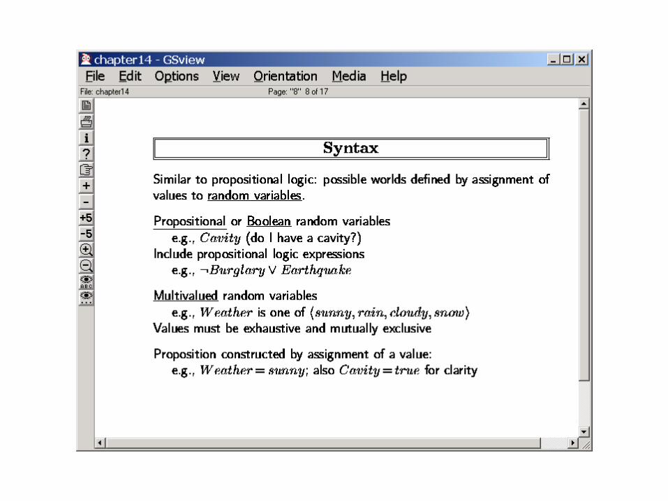
Need for modeling uncertainity

• Consider a simple scenario: You know that rain makes grass wet. Sprinklers also make grass wet. Wet grass means wet news paper. You woke up one morning and found that your newspaper (brought in by your trusted dog/kid/spouse) was wet

– Can we say something about whether it rained the previous day?

– Will logic allow you to do it?

• You hear the whooshing sound of the sprinklers outside the window– Does your belief in rain-the-previous-night change?

– Will logic capture this? • No—our “belief” in rain has reduced… that makes it “non-monotonic” change

• Standard logic is MONOTONIC

• (By the way, this is a form of inference called “explaining away”—increased belief in one explanation for a cause reduces the belief in the competing explanations).

“Monotonic Logics”

• Standard logic is monotonic– Given a database D and fact f, such that D|=f

• Adding new knowledge to D doesn’t reverse the entailment– D+d |= f if D|=f

• Plausible reasoning doesn’t have this property– Told that Tweety is a bird, we believe it will fly. Told that it is

an ostrich, we believe it doesn’t. Told that it is a magical ostrich, we believe it does…

– Probabilistic reasoning allows non-monotonicity

– (So does a class of logics called “default logics”—Chitta Baral is the Big Cheese in the default logic community).

Pot

ato

in th

e

Tailp

ipe p

robl

em

Qualification problem --impossible to enumerate all preconditionsRamification problem --impossible to enumerate all effects Frame problem --impossible to enumerate all that stays unchanged

If you know th

e full j

oint,

You can answ

er ANY query

TA ~TA

CA 0.04 0.06

~CA 0.01 0.89

P(CA & TA) =

P(CA) =

P(TA) =

P(CA V TA) =

P(CA|~TA) =

Lecture of 11/13

TA ~TA

CA 0.04 0.06

~CA 0.01 0.89

P(CA & TA) =

P(CA) =

P(TA) =

P(CA V TA) =

P(CA|~TA) =

Problem:

--Need too many

numbers…

Will we always need 2n numbers?

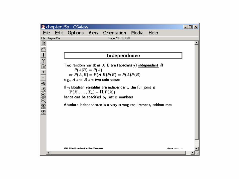
• If every pair of variables is independent of each other, then– P(x1,x2…xn)= P(xn)* P(xn-1)*…P(x1)– Need just n numbers!– But if our world is that simple, it would also be very uninteresting (nothing is

correlated with anything else!)

• We need 2n numbers if every subset of our n-variables are correlated together– P(x1,x2…xn)= P(xn|x1…xn-1)* P(xn-1|x1…xn-2)*…P(x1)– But that is too pessimistic an assumption on the world

• If our world is so interconnected we would’ve been dead long back…

A more realistic middle ground is that interactions between variables are contained to regions. --e.g. the “school variables” and the “home variables” interact only loosely (are independent for most practical purposes) -- Will wind up needing O(2k) numbers (k << n)

A be Anthrax; Rn be Runny NoseP(A|Rn) = P(Rn|A) P(A)/ P(Rn)

“Proof theory”

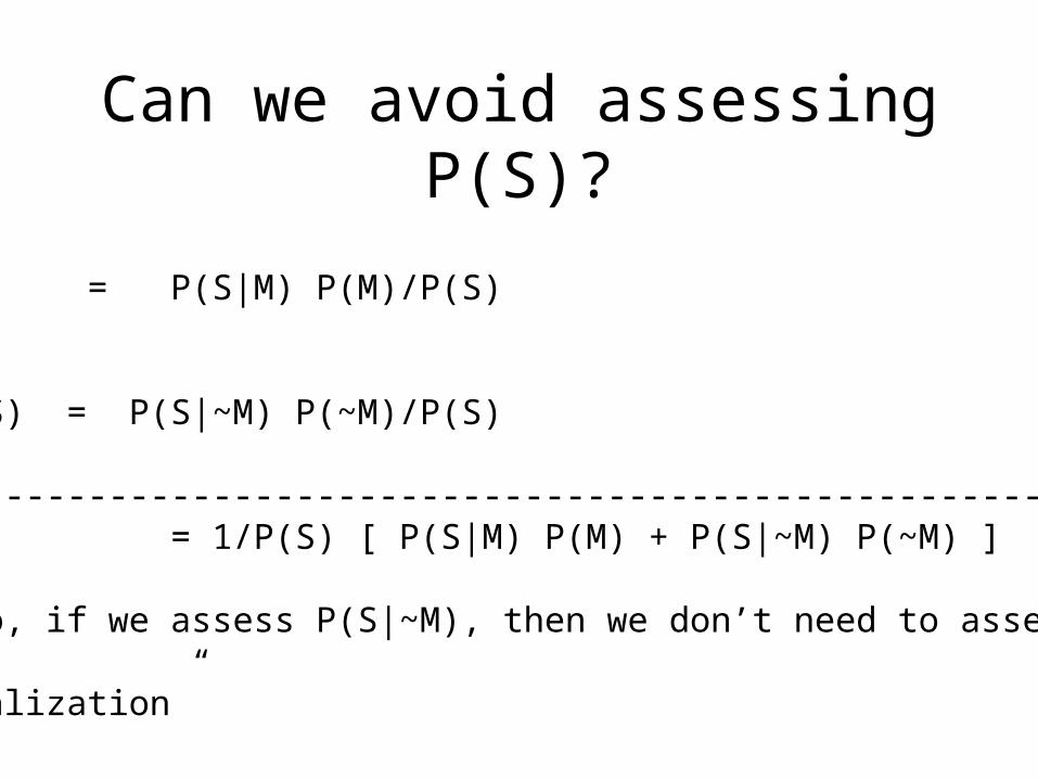
Can we avoid assessing P(S)?

P(M|S) = P(S|M) P(M)/P(S)

P(~M|S) = P(S|~M) P(~M)/P(S)

---------------------------------------------------------------- 1 = 1/P(S) [ P(S|M) P(M) + P(S|~M) P(~M) ] So, if we assess P(S|~M), then we don’t need to assess P(S)

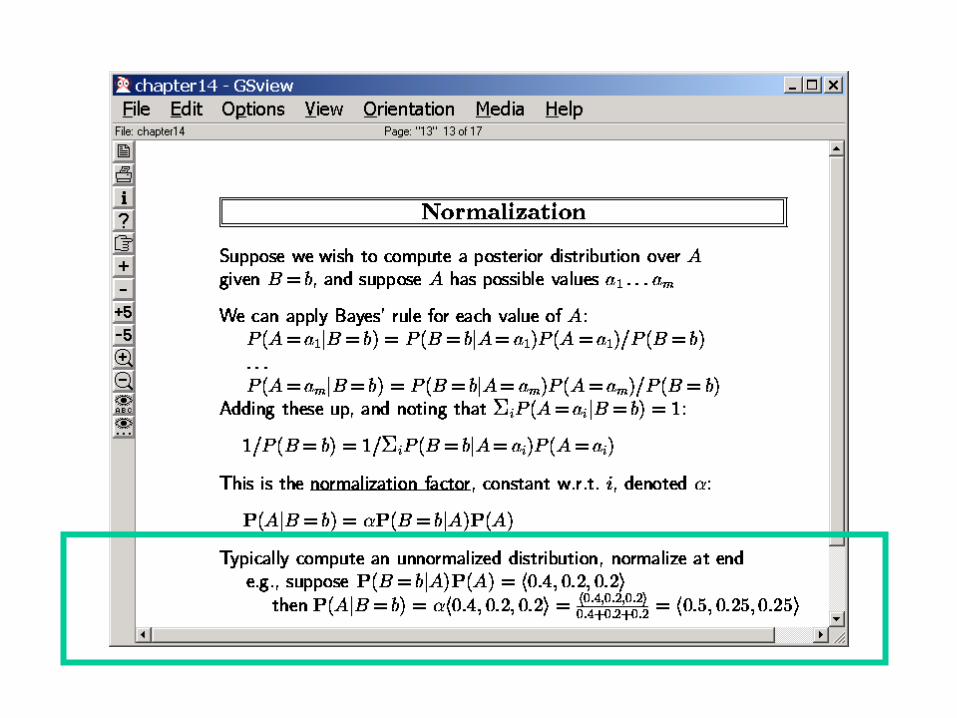
“Normalization”

What happens if there are multiple symptoms…?

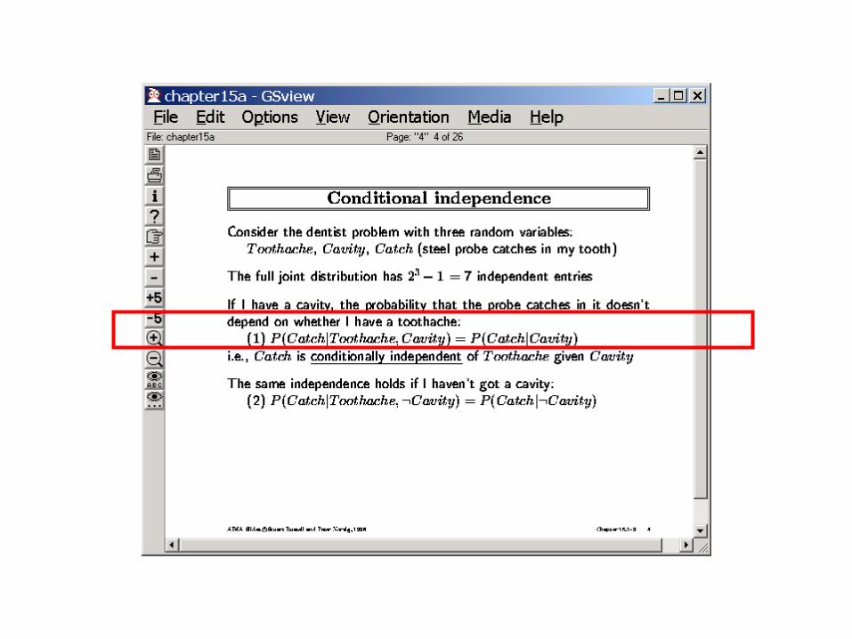
Patient walked in and complained of toothache

You assess P(Cavity|Toothache)

Now you try to probe the patients mouth with that steel thingie, and it catches…

How do we update our belief in Cavity?

P(Cavity|TA, Catch) = P(TA,Catch| Cavity) * P(Cavity)

P(TA,Catch)

= P(TA,Catch|Cavity) * P(Cavity)Need to know this!If n evidence variables,We will need 2n probabilities!

Conditional independenceTo the rescue Suppose P(TA,Catch|cavity) = P(TA|Cavity)*P(Catch|Cavity)

Lecture of 15th Nov, 2001.

Happy Dipavali

                                     

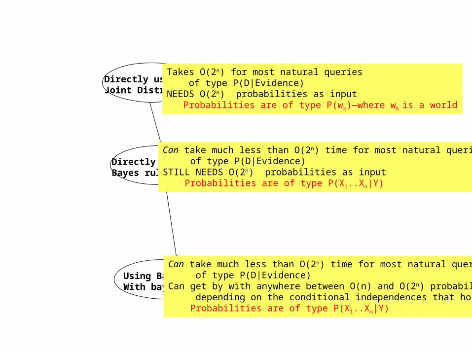
Directly usingJoint Distribution

Directly usingBayes rule

Using Bayes ruleWith bayes nets

Takes O(2n) for most natural queries of type P(D|Evidence)NEEDS O(2n) probabilities as input Probabilities are of type P(wk)—where wk is a world

Can take much less than O(2n) time for most natural queries of type P(D|Evidence)STILL NEEDS O(2n) probabilities as input Probabilities are of type P(X1..Xn|Y)

Can take much less than O(2n) time for most natural queries of type P(D|Evidence)Can get by with anywhere between O(n) and O(2n) probabilities depending on the conditional independences that hold. Probabilities are of type P(X1..Xn|Y)

Generalized bayes rule

P(A|B,e) = P(B|A,e) P(A|e) P(B|e)

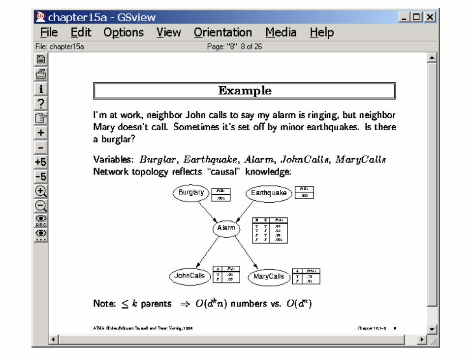
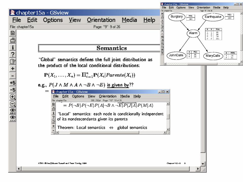
Alarm

P(A|J,M) =P(A)?

Burglary Earthquake

Markov Blanket

Each node is conditionally independent of all others given its Markov Blanket: Parents+Children+Children’s parents

Indep

enden

ce fr

om

Non-d

esce

dants

holds

Given ju

st th

e par

ents

Lecture of 11/16

Two parts:

Part 1: Practical issues in constructing Bayes networks

Part 2. Inference in Bayes networks

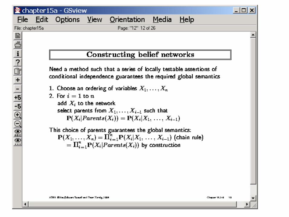
Part 1. Issues in constructing Bayes Nets

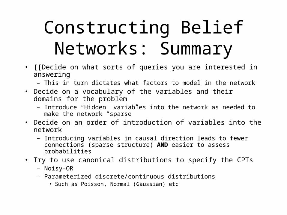
Constructing Belief Networks: Summary

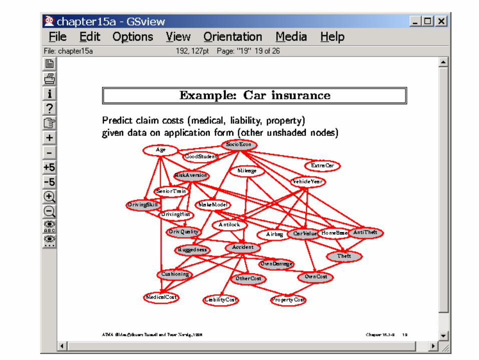
• [[Decide on what sorts of queries you are interested in answering– This in turn dictates what factors to model in the network

• Decide on a vocabulary of the variables and their domains for the problem– Introduce “Hidden” variables into the network as needed to make the

network “sparse”

• Decide on an order of introduction of variables into the network– Introducing variables in causal direction leads to fewer connections

(sparse structure) AND easier to assess probabilities

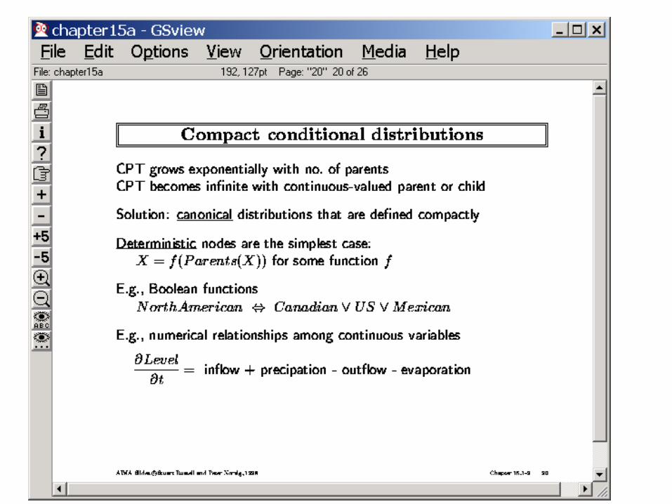
• Try to use canonical distributions to specify the CPTs– Noisy-OR– Parameterized discrete/continuous distributions

• Such as Poisson, Normal (Gaussian) etc

Constructing Belief Networks: Summary

• [[Decide on what sorts of queries you are interested in answering– This in turn dictates what factors to model in the network

• Decide on a vocabulary of the variables and their domains for the problem– Introduce “Hidden” variables into the network as needed to make the

network “sparse”

• Decide on an order of introduction of variables into the network– Introducing variables in causal direction leads to fewer connections

(sparse structure) AND easier to assess probabilities

• Try to use canonical distributions to specify the CPTs– Noisy-OR– Parameterized discrete/continuous distributions

• Such as Poisson, Normal (Gaussian) etc

Case Study: Pathfinder System

• Domain: Lymph node diseases– Deals with 60 diseases and 100 disease findings

• Versions:– Pathfinder I: A rule-based system with logical reasoning– Pathfinder II: Tried a variety of approaches for uncertainity

• Simple bayes reasoning outperformed – Pathfinder III: Simple bayes reasoning, but reassessed probabilities

– Parthfinder IV: Bayesian network was used to handle a variety of conditional dependencies.

• Deciding vocabulary: 8 hours• Devising the topology of the network: 35 hours• Assessing the (14,000) probabilities: 40 hours

– Physician experts liked assessing causal probabilites

• Evaluation: 53 “referral” cases– Pathfinder III: 7.9/10– Pathfinder IV: 8.9/10 [Saves one additional life in every 1000 cases!]– A more recent comparison shows that Pathfinder now outperforms experts who helped

design it!!

Part II. Inference in Bayes Nets

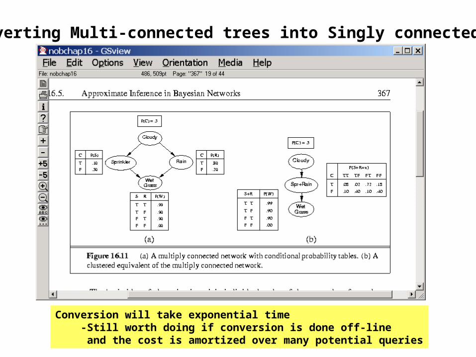
Converting Multi-connected trees into Singly connected trees

Conversion will take exponential time -Still worth doing if conversion is done off-line and the cost is amortized over many potential queries

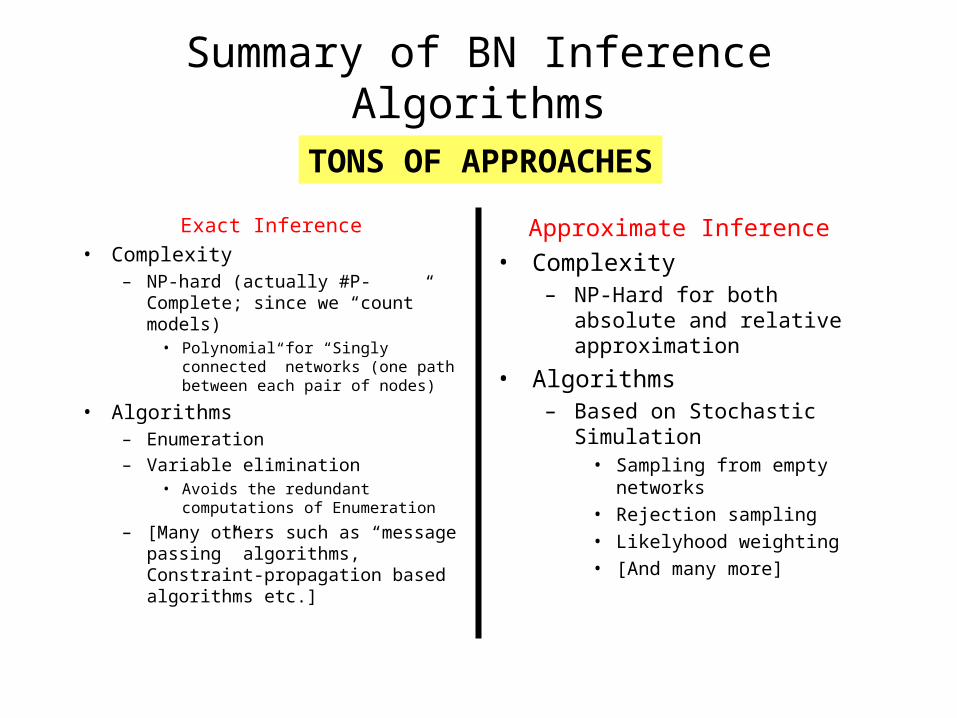
Summary of BN Inference Algorithms

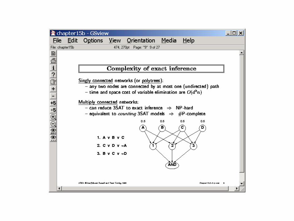
Exact Inference

• Complexity– NP-hard (actually #P-Complete;

since we “count” models)• Polynomial for “Singly

connected” networks (one path between each pair of nodes)

• Algorithms– Enumeration

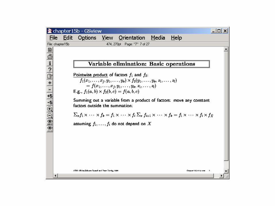
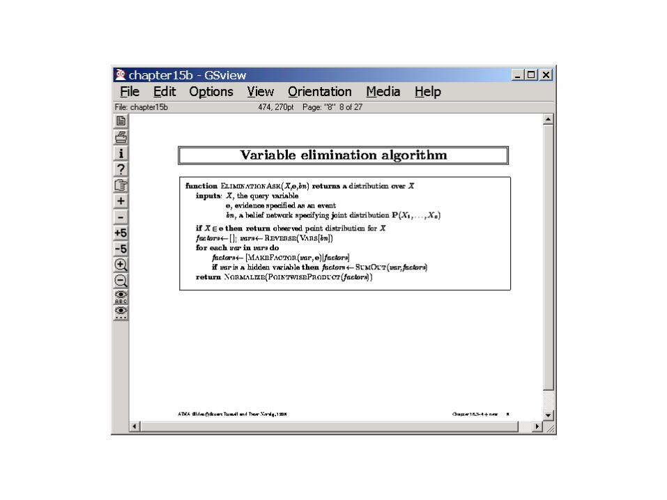
– Variable elimination• Avoids the redundant

computations of Enumeration

– [Many others such as “message passing” algorithms, Constraint-propagation based algorithms etc.]

Approximate Inference

• Complexity– NP-Hard for both absolute and

relative approximation

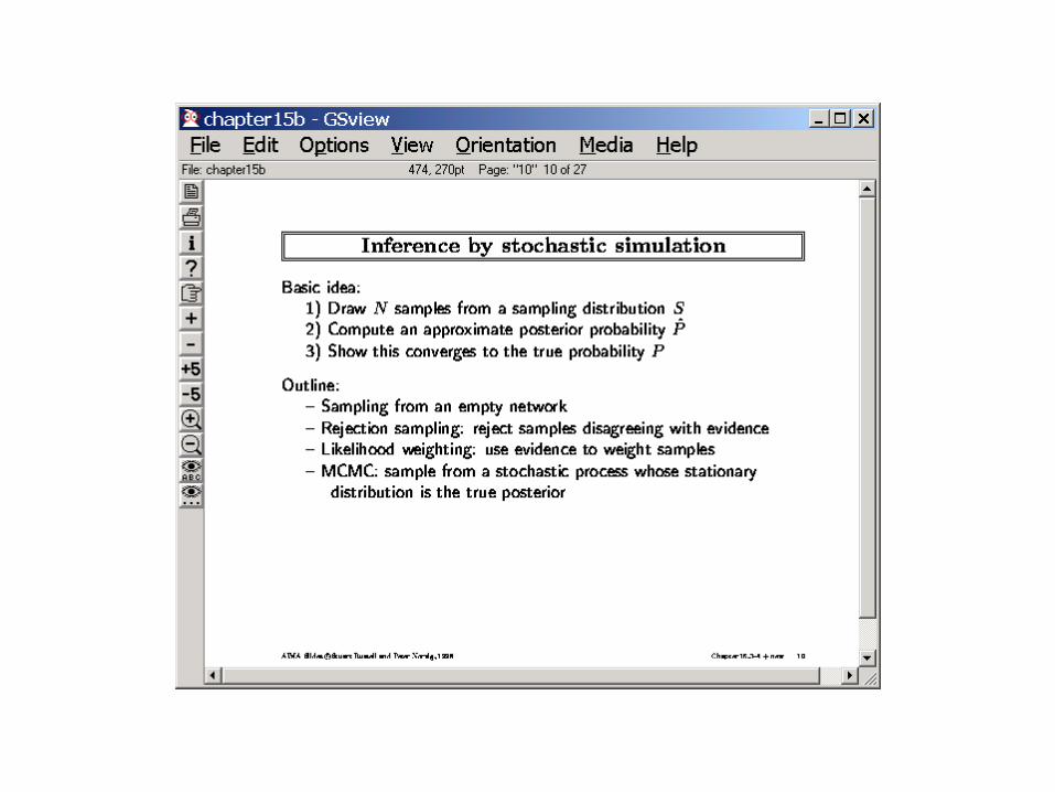
• Algorithms– Based on Stochastic Simulation

• Sampling from empty networks

• Rejection sampling

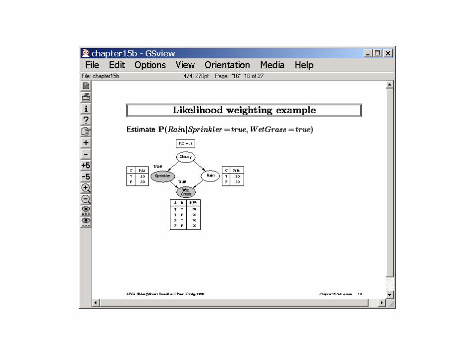
• Likelyhood weighting

• [And many more]

TONS OF APPROACHES

Inefficient (redundant) computations in Enumeration

Inefficient (redundant) computations in Enumeration

Repeated multiplications

Summary of BN Inference Algorithms

Exact Inference

• Complexity– NP-hard (actually #P-Complete;

since we “count” models)• Polynomial for “Singly

connected” networks (one path between each pair of nodes)

• Algorithms– Enumeration

– Variable elimination• Avoids the redundant

computations of Enumeration

– [Many others such as “message passing” algorithms, Constraint-propagation based algorithms etc.]

Approximate Inference

• Complexity– NP-Hard for both absolute and

relative approximation

• Algorithms– Based on Stochastic Simulation

• Sampling from empty networks

• Rejection sampling

• Likelyhood weighting

• [And many more]

TONS OF APPROACHES