probabilistic graphical modelsepxing/class/10708-15/slides/lecture29-distggm.pdf · rq,c2 rq...
TRANSCRIPT

School of Computer Science
Probabilistic Graphical Models
Distributed ADMM for Gaussian Graphical Models
Yaoliang Yu Lecture 29, April 29, 2015
1 © Eric Xing @ CMU, 2005-2015

Networks / Graphs
© Eric Xing @ CMU, 2005-2015 2

l Prior knowledge l Mom told me “A is connected to B”
l Estimate from data! l We have seen this in previous classes l Will see two more today
l Sometimes may also be interested in edge weights l An easier problem
l Real networks are BIG l Require distributed optimization
Where do graphs come from?
3 © Eric Xing @ CMU, 2005-2015

Structural Learning for completely observed
MRF (Recall) Data
),,( )()( 111 nxx …
),,( )()( Mn
M xx …1
…),,( )()( 22
1 nxx …
4 © Eric Xing @ CMU, 2005-2015
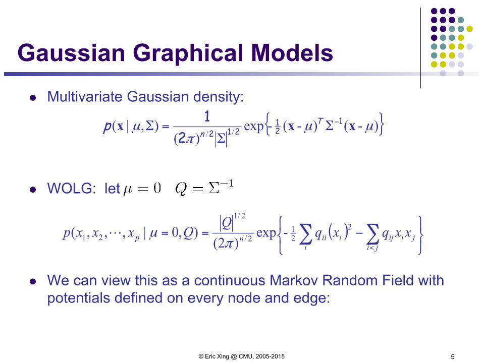
Gaussian Graphical Models l Multivariate Gaussian density:
l WOLG: let
l We can view this as a continuous Markov Random Field with potentials defined on every node and edge:
{ })-()-(-exp)(
),|( //µµ
πµ xxx 1
21
21221 −ΣΣ
=Σ Tn
p
( )⎭⎬⎫
⎩⎨⎧
−== ∑∑<
jiji
iji
iiinp xxqxqQ
Qxxxp 221
2/
2/1
21 -exp)2(
),0|,,,(π
µ!
5 © Eric Xing @ CMU, 2005-2015
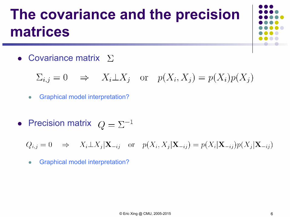
The covariance and the precision matrices
l Covariance matrix
l Graphical model interpretation?
l Precision matrix
l Graphical model interpretation?
6 © Eric Xing @ CMU, 2005-2015

Sparse precision vs. sparse covariance in GGM
2 1 3 5 4
⎟⎟⎟⎟⎟⎟
⎠
⎞
⎜⎜⎜⎜⎜⎜
⎝
⎛
=Σ−
5900094800083700072600061
1
⎟⎟⎟⎟⎟⎟
⎠
⎞
⎜⎜⎜⎜⎜⎜
⎝
⎛
−−
−−
−−
−−
−−
=Σ
080070120030150070040070010080120070100020130030010020030150150080130150100
.....
....................
)5(or )1(511
15 0 nbrsnbrsXXX ⊥⇔=Σ−
01551 =Σ⇔⊥ XX
⇒
7 © Eric Xing @ CMU, 2005-2015

Another example
l How to estimate this MRF? l What if p >> n
l MLE does not exist in general! l What about only learning a “sparse” graphical model?
l This is possible when s=o(n) l Very often it is the structure of the GM that is more interesting …
8 © Eric Xing @ CMU, 2005-2015

Recall lasso
9 © Eric Xing @ CMU, 2005-2015

Graph Regression (Meinshausen & Buhlmann’06)
Lasso: Neighborhood selection
10 © Eric Xing @ CMU, 2005-2015

Graph Regression
11 © Eric Xing @ CMU, 2005-2015
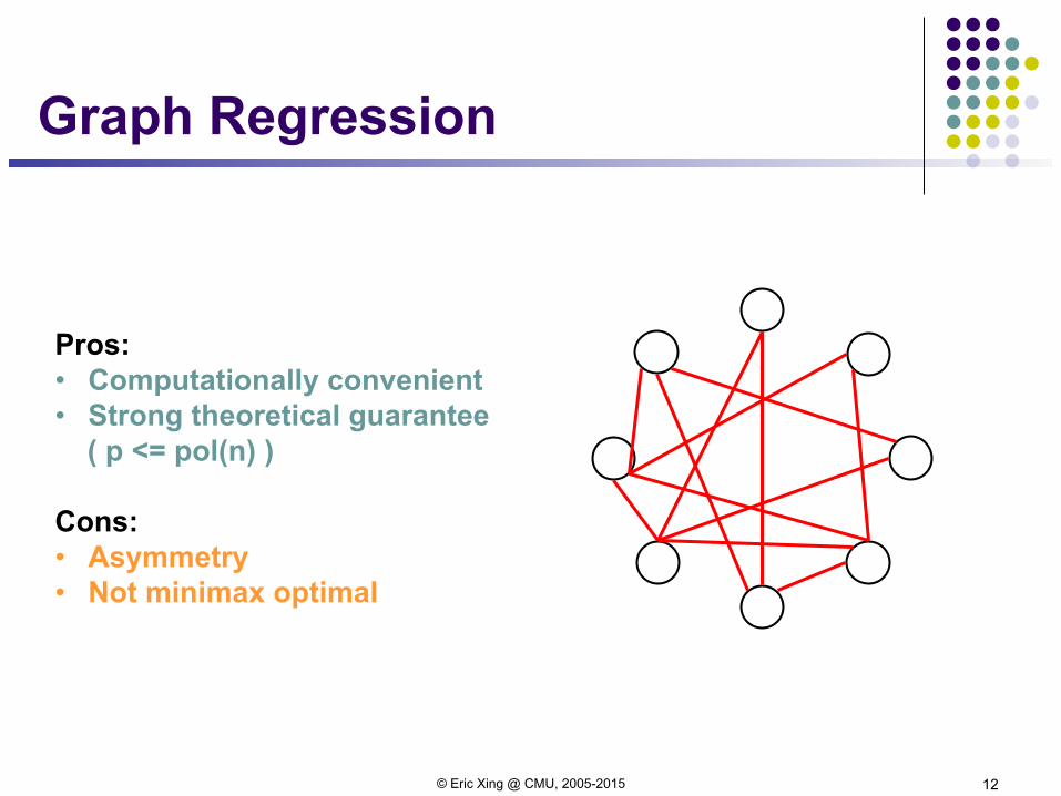
Graph Regression
Pros: • Computationally convenient • Strong theoretical guarantee
( p <= pol(n) )
Cons: • Asymmetry • Not minimax optimal
12 © Eric Xing @ CMU, 2005-2015

The regularized MLE (Yuan & Lin’07)
l S: sample covariance matrix, may be singular l ||Q||1: may exclude the diagonal l log det Q: implicitly force Q to be PSD symmetric
Pros
l Single step for estimating graph and inverse covariance l MLE!
Cons l Computationally challenging, partly solved by Glasso (Banergee et al’08,
Friedman et al’08)
© Eric Xing @ CMU, 2005-2015 13
min
Q� log detQ+ tr(QS) + �kQk1

Many many follow-ups
© Eric Xing @ CMU, 2005-2015 14

A closer look of RMLE
l Set derivative to 0:
l Can we (?!):
© Eric Xing @ CMU, 2005-2015 15
min
Q� log detQ+ tr(QS) + �kQk1
�Q�1 + S + � · sign(Q) = 0
kQ�1 � Sk1 �
minQ
kQk1 s.t. kQ�1 � Sk1 �

CLIME (Cai et al.’11)
l Further relaxation
l Constraint controls l Objective controls sparsity in Q l Q is not required to be PSD or symmetric
l Separable! LP!!! l Both objective and constraint are element-wise separable l Can be reformulated as LP
l Strong theoretical guarantee l Variations are minimax-optimal (Cai et al.’12, Liu & Wang’12)
© Eric Xing @ CMU, 2005-2015 16
minQ
kQk1 s.t. kSQ� Ik1 �
Q ⇡ S�1

But for BIG problems
l Standard solvers for LP can be slow l Embarrassingly parallel:
l Solve each column of Q independently in each core/machine
l Thanks for not having PSD constraint on Q l Still troublesome if S is big l Need to consider first-order methods
© Eric Xing @ CMU, 2005-2015 17
minQ
kQk1 s.t. kSQ� Ik1 �
minqi
kqik1 s.t. kSqi � eik1 �

© Eric Xing @ CMU, 2005-2015 18
A gentle introduction to alternating direction method of
multipliers (ADMM)

Optimization with coupling variables
l Numerically challenging because l Function f or g nonsmooth or constrained (i.e., can take value ) l Linear constraint couples the variables w and z l Large scale, interior point methods NA
l Naively alternating x and z does not work l Min w2 s.t. w + z = 1; optimum clearly is w = 0 l Start with say w = 1 à z = 0 à w = 1 à z = 0 …
l However, without coupling, can solve separately w and z l Idea: try to decouple vars in the constraint!
© Eric Xing @ CMU, 2005-2014
19
1
J uncoupled L coupled
where
Canonical form: minw,z
f(w) + g(z), s.t. Aw +Bz = c,w 2 Rm, z 2 Rp, A : Rm ! Rq, B : Rp ! Rq, c 2 Rq

Example: Empirical Risk Minimization (ERM)
l Each i corresponds to a training point (xi, yi) l Loss fi measures the fitness of the model parameter w
l least squares: l support vector machines: l boosting: l logistic regression:
l g is the regularization function, e.g. or l Vars coupled in obj, but not in constraint (none)
l Reformulate: transfer coupling from obj to constraint l Arrive at canonical form, allow unified treatment later
© Eric Xing @ CMU, 2005-2014
20
minw
g(w) +nX
i=1
fi(w)
�nkwk22 �nkwk1
fi(w) = (yi � w
>xi)
2
fi(w) = (1� yiw>xi)+
fi(w) = exp(�yiw>xi)
fi(w) = log(1 + exp(�yiw>xi))
L coupled

Why canonical form?
l ADMM algorithm (to be introduced shortly) excels at solving the canonical form l Canonical form is a general “template” for constrained problems
l ERM (and many other problems) can be converted to canonical form through variable duplication (see next slide)
© Eric Xing @ CMU, 2005-2013 21
minw
g(w) +nX
i=1
fi(w)ERM:
where
Canonical form: minw,z
f(w) + g(z), s.t. Aw +Bz = c,w 2 Rm, z 2 Rp, A : Rm ! Rq, B : Rp ! Rq, c 2 Rq

How to: variable duplication l Duplicate variables to achieve canonical form
l Global consensus constraint:
l All wi must (eventually) agree
l Downside: many extra variables, increase problem size l Implicitly maintain duplicated variables
© Eric Xing @ CMU, 2005-2014
minw
g(w) +nX
i=1
fi(w)
8i, wi = z
22
minv,z
g(z) +X
ifi(wi)
| {z }f(v)
, s.t. wi = z, 8i| {z }v�[I,...,I]>z=0
v = [w1, . . . , wn]>

Augmented Lagrangian
l Intro Lagrangian multiplier to decouple variables
l : augmented Lagrangian l More complicated min-max problem, but no coupling constraints
© Eric Xing @ CMU, 2005-2014
23
Lµ
min
w,zmax
�f(w) + g(z) + �>
(Aw +Bz� c) + µ2 kAw +Bz� ck22| {z }
Lµ(w,z;�)
�
where
Canonical form: minw,z
f(w) + g(z), s.t. Aw +Bz = c,w 2 Rm, z 2 Rp, A : Rm ! Rq, B : Rp ! Rq, c 2 Rq

Why Augmented Lagrangian? l Quadratic term gives numerical stability
l May lead to strong convexity in w or z l Faster convergence when strongly convex
l Allows larger step size (due to higher stability) l Prevents subproblems diverging to infinity (again, stability)
l But sometimes better to work with normal Lagrangian
© Eric Xing @ CMU, 2005-2013 24
min
w,zmax
�f(w) + g(z) + �>
(Aw +Bz� c) + µ2 kAw +Bz� ck22| {z }
Lµ(w,z;�)

ADMM Algorithm
© Eric Xing @ CMU, 2005-2014
25
l Fix dual , block coordinate descent on primal w, z
l Fix primal w, z, gradient ascent on dual
l Step size can be large, e.g. l Usually rescale to remove
⌘ ⌘ = µ⌘
min
w,zmax
�f(w) + g(z) + �>
(Aw +Bz� c) + µ2 kAw +Bz� ck22| {z }
Lµ(w,z;�)
�t+1 �t + ⌘(Awt+1 +Bzt+1 � c)
wt+1 argminw
Lµ(w, zt;�t)
zt+1 argminz
Lµ(wt+1, z;�t)
⌘ f(w) + µ2 kAw +Bzt � c+ �t/µk2
⌘ g(z) + µ2 kAwt+1 +Bz� c+ �t/µk2
�
�
� �/⌘

ERM revisited l Reformulate by duplicating variables
l ADMM x-step:
l Thanks to duplicating
© Eric Xing @ CMU, 2005-2013 26
• Completely decoupled • Parallelizable • Closed-form if fi is “simple”
minv,z
g(z) +X
ifi(wi)
| {z }f(v)
, s.t. wi = z, 8i| {z }v�[I,...,I]>z=0
wt+1 argminw
Lµ(w, zt;�t) ⌘ f(w) + µ2 kAw +Bzt � c+ �t/µk2
=X
i
fi(wi) +µ2 kwi � zt + �t
ik2

ADMM: History and Related l Augmented Lagrangian Method (ALM): solve w, z jointly even
though coupled l (Bertsekas'82) and refs therein
l Alternating Direction of Multiplier Method (ADMM): alternate w and z as previous slide l (Boyd et al.'10) and refs therein l Operator splitting for PDEs: Douglas, Peaceman, and Rachford (50s-70s) l Glowinsky et al.'80s, Gabay'83; Spingarn'85 l (Eckstein & Bertsekas'92; He et al.'02) in variational inequality l Lots of recent work.
© Eric Xing @ CMU, 2005-2014
27

ADMM: Linearization l Demanding step in each iteration of ADMM (similar for z): l Diagonal A: reduce to proximal map (more later) of f
l , soft-shrinkage:
l Non-diagonal A: no closed-form, messy inner loop l Instead, reduce to diagonal A by
l A single gradient step: l Or, linearize the quadratic at :
l Intuition: x re-computed in the next iteration anyways l No need for “perfect” x
© Eric Xing @ CMU, 2005-2014
28
x
t+1 argminx
L
µ
(x, zt
; yt
) = f(x) + g(zt) + y
>t (Ax+Bzt � c) + µ
2 kAx+Bzt � ck22
f(x) = kxk1 sign(x) · (|x|� µ)+
xt+1 xt � ⌘@f(xt) +A
>yt + µA
>(Axt +Bzt � c)
xt
x
t+1 argminx
f(x) + y
>t
Ax+ (x� x
t
)>µA>(Ax
t
+Bz
t
� c) + µ
2 kx� x
t
k22| {z }f(x)+
µ
2 kx�xt+A
>(Axt+Bzt�c+yt/µ)k22

Convergence Guarantees: Fixed-point theory
l Recall some definitions
l well-defined for convex f, non-expansive: l proximal map generalizes the Euclidean projection
l Lagrangian:
l ADMM = Douglas-Rachford splitting
l Fixed-point iteration! l convergence follows, e.g. (Bauschke & Combettes'13) l explains why dual y, not primal x or z, always converges
© Eric Xing @ CMU, 2005-2014
29
proximal map Pµf (w) := argmin
z
12µkz � wk22 + f(z)
reflection map Rµf (w) := 2Pµ
f (w)� w
kT (x)� T (y)k2 kx� yk2
L0(x, z; y) = minx
⇣f(x) + y
>Ax
⌘
| {z }d1(y)
+minz
⇣g(z) + y
>(Bz � c)⌘
| {z }d2(y)
w 12 (w + Rµ
d2(Rµ
d1(w))); y Pµ
d2(w)

© Eric Xing @ CMU, 2005-2015 30
ADMM for CLIME

Apply ADMM to CLIME
l Solve a block of columns of Q in each core/machine l E is the corresponding block in I
l Step 1: reduce to ADMM canonical form l Use variable duplicating
© Eric Xing @ CMU, 2005-2015 31
minQ
kQk1 s.t. kSQ� Ek1 �
minQ,Z
kQk1 s.t. kZ � Ek1 �, Z = SQ
minQ,Z
kQk1 + [kZ � Ek1 �] s.t. Z = SQ

Apply ADMM to CLIME (cont’)
l Step 2: Write out augmented Lagrangian
l Step 3: Perform primal-dual updates
© Eric Xing @ CMU, 2005-2015 32
Q argminQkQk1 +
⇢
2kSQ� Z + Y k2F
L(Q,Z;Y ) = kQk1 + [kZ � Ek1 �] + ⇢tr[(SQ� Z)Y ] +⇢
2kSQ� Zk2F
Z argminZ
[kZ � Ek1 �] +⇢
2kSQ� Z + Y k2F
= arg minkZ�Ek1�
⇢
2kSQ� Z + Y k2F
Y Y + SQ� Z

Apply ADMM to CLIME (cont’’)
l Step 4: Solve the subproblems l Lagrangian dual Y: trivial l Primal Z: projection to l_inf ball, separable, easy l Primal Q: easy if S is orthogonal, in general a lasso problem
l Bypass double loop by linearization l Intuition: wasteful to solve Q to death
l Soft-thresholding
l Putting things together
© Eric Xing @ CMU, 2005-2015 33
Q argminQkQk1 +
⇢
2kSQ� Z + Y k2F
Z argminZ
[kZ � Ek1 �] +⇢
2kSQ� Z + Y k2F
= arg minkZ�Ek1�
⇢
2kSQ� Z + Y k2F
Y Y + SQ� Z
minQ
kQk1 + ⇢tr(Q>S(Y + SQt � Z)) +⌘
2kQ�Qtk2F

Exploring structure l Expensive step in ADMM-CLIME:
l Matrix-matrix multiplication: SQ and alike
l If p >> n, S is size p x p but of rank at most n l Write S = AA’, and do A(A’Q)
l Matrix * matrix >> for loop of matrix * vector l Preferable to solve a balanced block of columns
© Eric Xing @ CMU, 2005-2015 34
A = [X1, . . . , Xn] 2 Rp⇥n
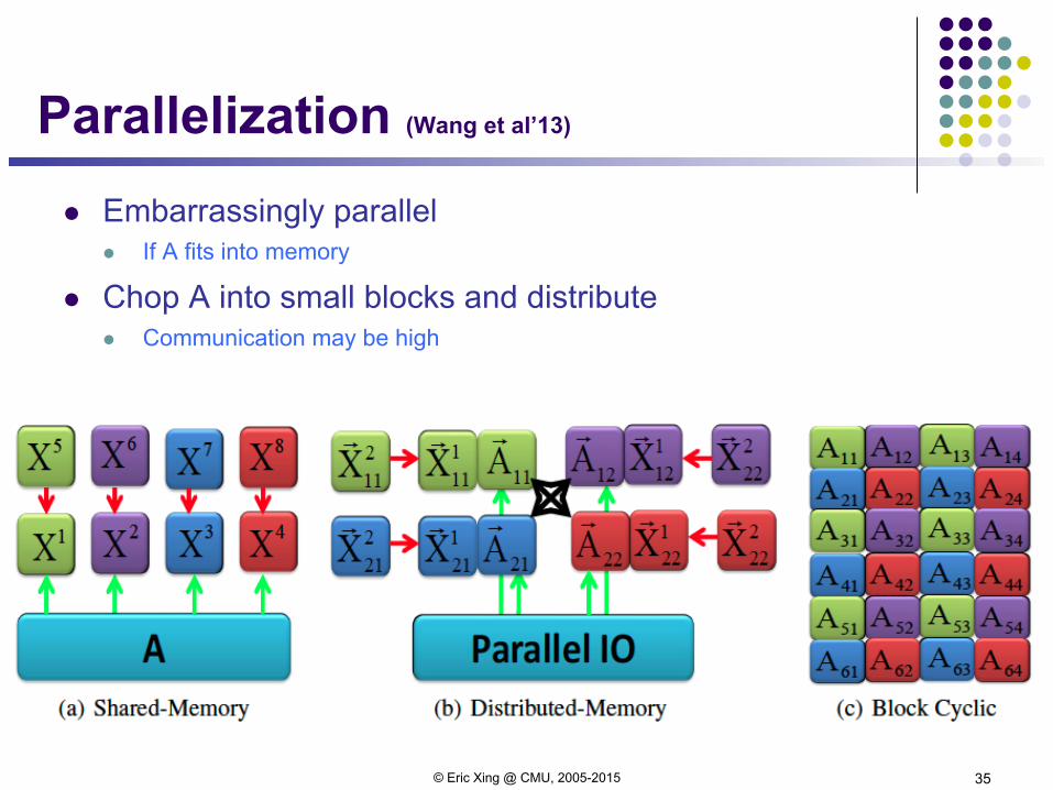
Parallelization (Wang et al’13)
© Eric Xing @ CMU, 2005-2015 35
l Embarrassingly parallel l If A fits into memory
l Chop A into small blocks and distribute l Communication may be high

Numerical results (Wang et al’13)
© Eric Xing @ CMU, 2005-2015 36

Numerical results cont’ (Wang et al’13)
© Eric Xing @ CMU, 2005-2015 37

© Eric Xing @ CMU, 2005-2015 38
Nonparanormal extensions

Nonparanormal (Liu et al.’09)
l fi: unknown monotonic functions l Observe X, but not Z l Independence preserved under transformations
l Can estimate fi first, then apply glasso on fi(Xi) l Estimating functions can be slow, nonparametric rate
© Eric Xing @ CMU, 2005-2015 39
Zi = fi(Xi), i = 1, . . . , p
(Z1, . . . , Zp) ⇠ N (0,⌃)
Xi ? Xj |Xrest () Zi ? Zj |Zrest () Qij = 0

A neat observation l Since fi is monotonic
l Zi,: comonotone / concordant with Xi,:
l Use rank estimator !
l Want , but do not observe Z l Maybe ???
© Eric Xing @ CMU, 2005-2015 40
Zi,1, Zi,2, . . . , Zi,n
Ri,1, Ri,2, . . . , Ri,n
Xi,1, Xi,2, . . . , Xi,n
⌃ij =1
n
nX
k=1
Zi,kZj,k?=
1
n
nX
k=1
Ri,kRj,k
⌃
Zi = fi(Xi), i = 1, . . . , p
(Z1, . . . , Zp) ⇠ N (0,⌃)

Kendall’s tau l Assuming no ties:
l Complexity of computing Kendall’s tau?
l Key:
l Genuine, asymptotically unbiased estimate of l is a contraction, preserving concentration
l After having , use whatever glasso, e.g., CLIME l Can also use other rank estimator, e.g., Spearman’s rho
© Eric Xing @ CMU, 2005-2015 41
⌧ij =1
n(n� 1)
X
k,`
sign[(Ri,k �Ri,`)(Rj,k �Rj,`)]
⌃ij = 2 sin(⇡
6E(⌧ij))⌃
t 7! 2 sin(⇡
6t)
⌃

Summary l Gaussian graphical model selection
l Neighborhood selection, Regularized MLE, CLIME l Implicit PSD vs. Explicit PSD
l Distributed ADMM l Generic procedure l Can distribute matrix product
l Nonparanormal Gaussian graphical model l Rank statistics l Plug-in estimator
© Eric Xing @ CMU, 2005-2015 42

References l Graph Lasso
l High-Dimensional Graphs and Variable Selection with the LASSO, Meinshausen and Buhlmann, Annals of Statistics, vol. 34, 2006
l Model Selection and Estimation in the Gaussian Graphical Model, Yuan and Lin, Biometrika, vol. 94, 2007 l A Constrained l_1 minimization Approach for Sparse Precision Matrix Estimation, Cai et al., Journal of the American
Statistical Association, 2011 l Model Selection Through Sparse Maximum Likelihood Estimation for Multivariate Gaussian or Binary Data, Banerjee et
al, Journal of Machine Learning Research, 2008 l Sparse Inverse Covariance Estimation with the Graphical Lasso, Friedman et al., Biostatistics, 2008
l Nonparanormal l The Nonparanormal: Semiparametric Estimation of High Dimensional Undirected Graphs, Han Liu et al., Journal of
Machine Learning Research, 2009 l Regularized Rank-based Estimation of High-Dimensional Nonparanormal Graphical Models, Lingzhou Xue and Hui
Zou, Annals of Statistics, vol. 40, 2012 l High-Dimensional Semiparametric Gaussian Copula Graphical Models, Han Liu et al., Annals of Statistics, vol. 40,
2012 l ADMM
l Large Scale Distributed Sparse Precision Estimation, Wang et al., NIPS 2013 l Distributed Optimization and Statistical Learning via the Alternating Direction Method of Multipliers, Boyd et al.,
Foundation and Trends in Machine Learning, 2011
© Eric Xing @ CMU, 2005-2015 43