School of Computer Science

Probabilistic Graphical Models

Learning Partially Observed GM: the Expectation-Maximization

algorithm

Eric XingLecture 9, February 12, 2014

Reading: MJ Chap 9, and 111© Eric Xing @ CMU, 2005-2014

Partially observed GMs Speech recognition

A AA AX2 X3X1 XT

Y2 Y3Y1 YT...

...

2© Eric Xing @ CMU, 2005-2014

Partially observed GM Biological Evolution

AGAGAC

3© Eric Xing @ CMU, 2005-2014

Mixture Models

4© Eric Xing @ CMU, 2005-2014

Mixture Models, con'd A density model p(x) may be multi-modal. We may be able to model it as a mixture of uni-modal

distributions (e.g., Gaussians). Each mode may correspond to a different sub-population

(e.g., male and female).

5© Eric Xing @ CMU, 2005-2014

Unobserved Variables A variable can be unobserved (latent) because:

it is an imaginary quantity meant to provide some simplified and abstractive view of the data generation process e.g., speech recognition models, mixture models …

it is a real-world object and/or phenomena, but difficult or impossible to measure e.g., the temperature of a star, causes of a disease, evolutionary ancestors …

it is a real-world object and/or phenomena, but sometimes wasn’t measured, because of faulty sensors, etc.

Discrete latent variables can be used to partition/cluster data into sub-groups.

Continuous latent variables (factors) can be used for dimensionality reduction (factor analysis, etc).

6© Eric Xing @ CMU, 2005-2014

Gaussian Mixture Models (GMMs) Consider a mixture of K Gaussian components:

This model can be used for unsupervised clustering. This model (fit by AutoClass) has been used to discover new kinds of stars in

astronomical data, etc.

k kkkn xNxp ),|,(),(

mixture proportion mixture component

7© Eric Xing @ CMU, 2005-2014

Gaussian Mixture Models (GMMs) Consider a mixture of K Gaussian components:

Z is a latent class indicator vector:

X is a conditional Gaussian variable with a class-specific mean/covariance

The likelihood of a sample:

k

zknn

knzzp ):(multi)(

)-()-(-exp)(

),,|( // knkT

knk

mknn xxzxp

1

21

212211

k kkkz kz

kknz

k

kkk

n

xNxN

zxpzpxp

n

kn

kn ),|,(),:(

),,|,()|(),(

11mixture proportion

mixture component

Z

X

8© Eric Xing @ CMU, 2005-2014

Why is Learning Harder? In fully observed iid settings, the log likelihood decomposes

into a sum of local terms (at least for directed models).

With latent variables, all the parameters become coupled together via marginalization

),|(log)|(log)|,(log);( xzc zxpzpzxpD l

z

xzz

c zxpzpzxpD ),|()|(log)|,(log);( l

9© Eric Xing @ CMU, 2005-2014

Recall MLE for completely observed data

Data log-likelihood

MLE

What if we do not know zn?

Cxzz

xN

zxpzpxzpD

n kkn

kn

n kk

kn

n k

zkn

n k

zk

nnn

nn

nn

kn

kn

22

1 )-(log

),;(loglog

),,|()|(log),(log);(

2

θl

Toward the EM algorithm

zi

xiN

),;(maxargˆ , DMLEk θl

);(maxargˆ , DMLEk θl

);(maxargˆ , DMLEk θl

nkn

n nkn

MLEk zxz

,ˆ

10© Eric Xing @ CMU, 2005-2014

Question “ … We solve problem X using Expectation-Maximization …”

What does it mean?

E What do we take expectation with? What do we take expectation over?

M What do we maximize? What do we maximize with respect to?

11© Eric Xing @ CMU, 2005-2014

Recall: K-means

)()(maxarg )()()()( tkn

tk

Ttknk

tn xxz 1

nt

n

n nt

ntk kz

xkz),(

),()(

)()(

1

12© Eric Xing @ CMU, 2005-2014

Expectation-Maximization Start:

"Guess" the centroid k and coveriance k of each of the K clusters

Loop

13© Eric Xing @ CMU, 2005-2014

Example: Gaussian mixture model A mixture of K Gaussians:

Z is a latent class indicator vector

X is a conditional Gaussian variable with class-specific mean/covariance

The likelihood of a sample:

The expected complete log likelihood

Zn

XnN

k

zknn

knzzp ):(multi)(

)-()-(-exp)(

),,|( // knkT

knk

mk

nn xxzxp

121

212211

k kkkz kz

kknz

k

kkk

n

xNxN

zxpzpxp

n

kn

kn ),|,(),:(

),,|,()|(),(

11

n kkknk

Tkn

kn

n kk

kn

nxzpnn

nxzpnc

Cxxzz

zxpzpzx

log)()(21log

),,|(log)|(log),;(

1

)|()|(

θl

14© Eric Xing @ CMU, 2005-2014

We maximize iteratively using the following iterative procedure:

─ Expectation step: computing the expected value of the sufficient statistics of the hidden variables (i.e., z) given current est. of the parameters (i.e., and ).

Here we are essentially doing inference

i

ti

tin

ti

tk

tkn

tkttk

nq

kn

tkn xN

xNxzpz t ),|,(),|,(),,|1( )()()(

)()()()()()(

)(

)(θcl

E-step

15© Eric Xing @ CMU, 2005-2014

We maximize iteratively using the following iterative procudure:

─ Maximization step: compute the parameters under current results of the expected value of the hidden variables

This is isomorphic to MLE except that the variables that are hidden are replaced by their expectations (in general they will by replaced by their corresponding "sufficient statistics")

)(θcl

M-step

1 s.t. , ,0)( ,)(maxarg

)(*

k

*

)(

Nn

NNz

kll

kntk

nn q

kn

k

kcck

t

k

θθ

ntk

n

n ntk

ntkk

xl )(

)()1(* ,)(maxarg

θ

ntk

n

nTt

knt

kntk

ntkk

xxl )(

)1()1()()1(* ))((

,)(maxarg

θ T

T

T

xxxx

AA

A A

Alog

:Fact

1

1

16© Eric Xing @ CMU, 2005-2014

Compare: K-means and EM

K-means In the K-means “E-step” we do hard

assignment:

In the K-means “M-step” we update the means as the weighted sum of the data, but now the weights are 0 or 1:

EM E-step

M-step

)()(maxarg )()()()( tkn

tk

Ttknk

tn xxz 1

nt

n

n nt

ntk kz

xkz),(

),()(

)()(

1

The EM algorithm for mixtures of Gaussians is like a "soft version" of the K-means algorithm.

it

it

int

i

tk

tkn

tkttk

n

q

kn

tkn

xNxNxzp

z t

),|,(),|,(),,|1( )()()(

)()()()()(

)()(

ntk

n

n ntk

ntk

x)(

)()1(

17© Eric Xing @ CMU, 2005-2014

Theory underlying EM What are we doing?

Recall that according to MLE, we intend to learn the model parameter that would have maximize the likelihood of the data.

But we do not observe z, so computing

is difficult!

What shall we do?

z

xzz

c zxpzpzxpD ),|()|(log)|,(log);( l

18© Eric Xing @ CMU, 2005-2014

Complete & Incomplete Log Likelihoods Complete log likelihood

Let X denote the observable variable(s), and Z denote the latent variable(s). If Z could be observed, then

Usually, optimizing lc() given both z and x is straightforward (c.f. MLE for fully observed models).

Recalled that in this case the objective for, e.g., MLE, decomposes into a sum of factors, the parameter for each factor can be estimated separately.

But given that Z is not observed, lc() is a random quantity, cannot be maximized directly.

Incomplete log likelihoodWith z unobserved, our objective becomes the log of a marginal probability:

This objective won't decouple

)|,(log),;(def

zxpzxc l

z

c zxpxpx )|,(log)|(log);( l

19© Eric Xing @ CMU, 2005-2014

Expected Complete Log Likelihood

z

qc zxpxzqzx )|,(log),|(),;(def

l

z

z

z

xzqzxpxzq

xzqzxpxzq

zxpxpx

)|()|,(log)|(

)|()|,()|(log

)|,(log

)|(log);(

l

qqc Hzxx ),;();( ll

For any distribution q(z), define expected complete log likelihood:

A deterministic function of Linear in lc() --- inherit its factorizabiility Does maximizing this surrogate yield a maximizer of the likelihood?

Jensen’s inequality

20© Eric Xing @ CMU, 2005-2014

Lower Bounds and Free Energy For fixed data x, define a functional called the free energy:

The EM algorithm is coordinate-ascent on F : E-step:

M-step:

);()|(

)|,(log)|(),(def

xxzq

zxpxzqqFz

l

),(maxarg t

q

t qFq 1

),(maxarg ttt qF

11

21© Eric Xing @ CMU, 2005-2014

E-step: maximization of expected lc w.r.t. q Claim:

This is the posterior distribution over the latent variables given the data and the parameters. Often we need this at test time anyway (e.g. to perform classification).

Proof (easy): this setting attains the bound l(;x)F(q, )

Can also show this result using variational calculus or the fact that

),|(),(maxarg tt

q

t xzpqFq 1

);()|(log

)|(log)|(

),()|,(

log),()),,((

xxp

xpxzq

xzpzxpxzpxzpF

ttz

t

zt

tttt

l

),|(||KL),();( xzpqqFx l

22© Eric Xing @ CMU, 2005-2014

E-step plug in posterior expectation of latent variables Without loss of generality: assume that p(x,z|) is a

generalized exponential family distribution:

Special cases: if p(X|Z) are GLIMs, then

The expected complete log likelihood under is

)(),(

)()|,(log),|(),;(

),|(

Azxf

Azxpxzqzx

ixzqi

ti

z

ttq

tc

t

t

1l

i

ii zxfzxhZ

zxp ),(exp),()(

),(

1

)()(),( xzzxf iTii

),|( tt xzpq 1

)()()(),|(

GLIM~

Axzi

ixzqiti

p

t 23© Eric Xing @ CMU, 2005-2014

M-step: maximization of expected lc w.r.t. Note that the free energy breaks into two terms:

The first term is the expected complete log likelihood (energy) and the second term, which does not depend on , is the entropy.

Thus, in the M-step, maximizing with respect to for fixed qwe only need to consider the first term:

Under optimal qt+1, this is equivalent to solving a standard MLE of fully observed model p(x,z|), with the sufficient statistics involving z replaced by their expectations w.r.t. p(z|x,).

qqc

zz

z

Hzx

xzqxzqzxpxzqxzq

zxpxzqqF

),;(

)|(log)|()|,(log)|()|(

)|,(log)|(),(

l

zqc

t zxpxzqzx t )|,(log)|(maxarg),;(maxarg

11 l

24© Eric Xing @ CMU, 2005-2014

Example: HMM Supervised learning: estimation when the “right answer” is known

Examples: GIVEN: a genomic region x = x1…x1,000,000 where we have good

(experimental) annotations of the CpG islandsGIVEN: the casino player allows us to observe him one evening,

as he changes dice and produces 10,000 rolls

Unsupervised learning: estimation when the “right answer” is unknown Examples:

GIVEN: the porcupine genome; we don’t know how frequent are the CpG islands there, neither do we know their composition

GIVEN: 10,000 rolls of the casino player, but we don’t see when he changes dice

QUESTION: Update the parameters of the model to maximize P(x|) --- Maximal likelihood (ML) estimation

25© Eric Xing @ CMU, 2005-2014

Hidden Markov Model: from static to dynamic mixture models

Dynamic mixture

A AA AX2 X3X1 XT

Y2 Y3Y1 YT...

...

Static mixture

AX1

Y1

NThe sequence:

The underlying source:

Phonemes,

Speech signal,

sequence of rolls,

dice,

26© Eric Xing @ CMU, 2005-2014

The Baum Welch algorithm The complete log likelihood

The expected complete log likelihood

EM The E step

The M step ("symbolically" identical to MLE)

n

T

ttntn

T

ttntnnc xxpyypypp

1211 )|()|()(log),(log),;( ,,,,,yxyxθl

n

T

tkiyp

itn

ktn

n

T

tjiyyp

jtn

itn

niyp

inc byxayyy

ntnntntnnn 1211

11,)|(,,,)|,(,,)|(, logloglog),;(

,,,, xxxyxθ l

)|( ,,, nitn

itn

itn ypy x1

)|,( ,,,,,, n

jtn

itn

jtn

itn

jitn yypyy x1111

n

T

ti

tn

n

T

tjitnML

ija 1

1

2

,

,,

n

T

ti

tn

ktnn

T

ti

tnMLik

xb 1

1

1

,

,,

Nn

inML

i 1,

27© Eric Xing @ CMU, 2005-2014

Unsupervised ML estimation Given x = x1…xN for which the true state path y = y1…yN is

unknown,

EXPECTATION MAXIMIZATION

0. Starting with our best guess of a model M, parameters :

1. Estimate Aij , Bik in the training data How? , ,

2. Update according to Aij , Bik

Now a "supervised learning" problem3. Repeat 1 & 2, until convergence

This is called the Baum-Welch Algorithm

We can get to a provably more (or equally) likely parameter set each iteration

ktntn

itnik xyB ,, ,

tnjtn

itnij yyA

, ,, 1

28© Eric Xing @ CMU, 2005-2014

EM for general BNswhile not converged

% E-stepfor each node i

ESSi = 0 % reset expected sufficient statisticsfor each data sample n

do inference with Xn,H

for each node i

% M-stepfor each node i

i := MLE(ESSi )

)|(,,,,

),( HnHni xxpninii xxSSESS

29© Eric Xing @ CMU, 2005-2014

Summary: EM Algorithm A way of maximizing likelihood function for latent variable models.

Finds MLE of parameters when the original (hard) problem can be broken up into two (easy) pieces:

1. Estimate some “missing” or “unobserved” data from observed data and current parameters.

2. Using this “complete” data, find the maximum likelihood parameter estimates.

Alternate between filling in the latent variables using the best guess (posterior) and updating the parameters based on this guess:

E-step: M-step:

In the M-step we optimize a lower bound on the likelihood. In the E-step we close the gap, making bound=likelihood.

),(maxarg t

q

t qFq 1

),(maxarg ttt qF

11

30© Eric Xing @ CMU, 2005-2014

Conditional mixture model: Mixture of experts

We will model p(Y |X) using different experts, each responsible for different regions of the input space. Latent variable Z chooses expert using softmax gating function:

Each expert can be a linear regression model: The posterior expert responsibilities are

xxzP Tk Softmax)( 1 21 k

Tk

k xyzxyP ,;),( N

j jjj

jkkk

kk

xypxzpxypxzp

yxzP),,()(

),,()(),,( 2

2

11

1

31© Eric Xing @ CMU, 2005-2014

EM for conditional mixture model Model:

The objective function

EM:

E-step:

M-step: using the normal equation for standard LR , but with the data

re-weighted by (homework) IRLS and/or weighted IRLS algorithm to update {kkk} based on data pair

(xn,yn), with weights (homework?)

),,,|(),|()( ik

kk xzypxzpxyP 11

j jjnnjn

jn

kknnknkn

nnk

ntk

n xypxzpxypxzp

yxzP),,()(

),,()(),,()(

2

2

11

1

θ

n kk

k

nTknk

nn k

nTk

kn

nyxzpnnn

nyxzpnnc

Cxyzxz

zxypxzpzyx

22

),|(),|(

log)-(21)softmax(log

),,,|(log),|(log),,;(

θl

YXXX TT 1 )(

)(tkn 32© Eric Xing @ CMU, 2005-2014

Hierarchical mixture of experts

This is like a soft version of a depth-2 classification/regression tree. P(Y |X,G1,G2) can be modeled as a GLIM, with parameters

dependent on the values of G1 and G2 (which specify a "conditional path" to a given leaf in the tree).

33© Eric Xing @ CMU, 2005-2014

Mixture of overlapping experts

By removing the X Z arc, we can make the partitions independent of the input, thus allowing overlap.

This is a mixture of linear regressors; each subpopulation has a different conditional mean.

j jjj

jkkk

kk

xypzpxypzp

yxzP),,()(

),,()(),,( 2

2

11

1

34© Eric Xing @ CMU, 2005-2014

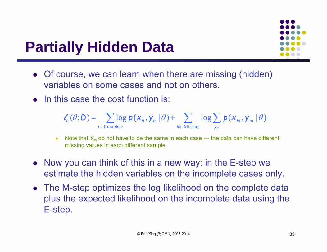
Partially Hidden Data Of course, we can learn when there are missing (hidden)

variables on some cases and not on others. In this case the cost function is:

Note that Ym do not have to be the same in each case --- the data can have different missing values in each different sample

Now you can think of this in a new way: in the E-step we estimate the hidden variables on the incomplete cases only.

The M-step optimizes the log likelihood on the complete data plus the expected likelihood on the incomplete data using the E-step.

MissingComplete

)|,(log)|,(log);(m y

mmn

nncm

yxpyxpD l

35© Eric Xing @ CMU, 2005-2014

EM Variants Sparse EM:

Do not re-compute exactly the posterior probability on each data point under all models, because it is almost zero. Instead keep an “active list” which you update every once in a while.

Generalized (Incomplete) EM: It might be hard to find the ML parameters in the M-step, even given the completed data. We can still make progress by doing an M-step that improves the likelihood a bit (e.g. gradient step). Recall the IRLS step in the mixture of experts model.

36© Eric Xing @ CMU, 2005-2014

A Report Card for EM Some good things about EM:

no learning rate (step-size) parameter automatically enforces parameter constraints very fast for low dimensions each iteration guaranteed to improve likelihood

Some bad things about EM: can get stuck in local minima can be slower than conjugate gradient (especially near convergence) requires expensive inference step is a maximum likelihood/MAP method

37© Eric Xing @ CMU, 2005-2014