probabilistic comparison of survival analysis models using...
TRANSCRIPT

LOGO
Probabilistic comparison of survival analysis models using simulation and cancer data
Statistical research team
Department of Mathematics and StatisticsUniversity of South Florida

Part 1Objective
By using Monte Carlo simulation, we want to evaluate uncensored survival data by using the most popular ways including Kaplan-Meier (KM) and Cox PH model and compare them with Kernel density (KD) and parametric model.
We want to validate these three ways by using real cancer data and we are interested to see if some way is better than others and based on that give some recommendations.

Parametric Analysis
We begin with the underlying failure distribution to be gamma with two parameters andHere we choose n=300 because when n=300 the MLE has already converged to the true value with small standard error.
Survival function is
True S(t)
Fitted S(t)
)3(
)2
,3(
1S(t,3,2)t
t
)3.0448746(
)1.941165,3.0448746(
1)ˆ,ˆ(t,St
t
0.3 0.5

Hazard function
Support ,
True h(t)
Fitted h(t)
is the gamma function and is the incomplete gamma function.
0t 0
)3()3(
th(t)
2
t
te
)3.0448746()3.0448746(
t(t)h
2.0448746
t
te
)(x

Graphical form n=300
We can see the Survival curve of true stat of nature and parametric gamma with MLE of and is close.
The survival plot is
3.0448746ˆ 0.5151546ˆ
0 5 10 15
0.0
0.2
0.4
0.6
0.8
1.0
time
S(t
)
true plot
fitted plot
)(S t

Cumulative Hazard plot
0 5 10 15
01
23
45
time
H(t
)
true plot
fitted plot
)(H t

Probability residual analysis
Consider the difference between true and parameter curve as our probability residual then mean of the probability residual is -0.006250685 with standard deviation is 0.003213453 and standard error is 0.0001855288.

Kaplan-Meier (KM) method
Survival function of Kaplan-Meier is
Cumulative Hazard function
tti
ni
dinit
)(S
)-ln()(H
tti
ni
dinit

For n=300 the true survival plot and KM survival plot
0 5 10 15
0.0
0.2
0.4
0.6
0.8
1.0
time
S(t
)
fitted plot blue
true plot red
)(S t

Cumulative Hazard function plot
0 5 10 15
01
23
45
6
time
H(t
)
fitted plot blue
true plot red
)(H t

Probability residual analysis
Consider the difference between true and parameter curve as our probability residual then mean of the probability residual is -0.007361148with standard deviation is 0.01458173 and standard error is 0.0008418766. Clearly the parametric way is much better than KM.

Kernel Density Analysis
probability density function is
Where K is a kernel and h is the optimal bandwidth.
Survival function
Hazard function
N
i
ih
h
xxK
Nhxf
1
)(1
)(ˆ
xX
N
i
ih
h
xxK
Nhx
1
)(1
1)(S
xX
N
i
i
N
i
i
h
h
xxK
Nh
h
xxK
Nhx
1
1
)(1
1
)(1
)(h

Detail and
Here is the detail of S(t) and h(t)
xX
N
i
ih
n
xIQRxSD
xx
n
xIQRxSDN
x1
2
5
1
5
1
)
34.1
))(),((1.06min(-1
4
3
34.1
))(),((1.06min
11)(S )(
xX
N
i
i
N
i
i
h
n
xIQRxSD
xx
n
xIQRxSDN
n
xIQRxSD
xx
n
xIQRxSDN
x
1
2
5
1
5
1
1
2
5
1
5
1
)
34.1
))(),((1.06min(-1
4
3
34.1
))(),((1.06min
11
)
34.1
))(),((1.06min(-1
4
3
34.1
))(),((1.06min
1
)(h
)(
)(
)(h )(S tt

Survival plot
0 5 10 15
0.0
0.2
0.4
0.6
0.8
1.0
time
S(t
)
ture red
KD blue
)(S t

Cumulative Hazard function
0 5 10 15
01
23
45
6
time
H(t
)
ture red
KD blue
)(H t

Probability residual analysis
Consider the difference between true and parameter curve as our probability residual then mean of the probability residual is -0.007816693 with standard deviation is 0.007590435 and standard error is 0.000438234.
Mean SD SE Rank of SE
Parametric -0.00625 0.0032 0.00018 #1
Kaplan-Meier -0.0074 0.0145 0.00084 #3
Kernel density -0.0078 0.0075 0.00043 #2

Partial Conclusion
From the above table we can clearly to see that parametric is much better than other two. This verifies with what we expected.
For difficult data, which means we can not proceed to go parametric way, we are better of going to KD method instead of popular KM method.
The reason is KM and KD is tie on mean of probability residual but KD’s standard deviation and standard error is about 50% of KM way. Therefore KD should be the priority to choose for nonparametric way in this situation. (If the true is two parameter Gamma and by this random data set).

Model validation with real breast cancer data
We have known that parametric way will for sure be best. Then the next question is for KD, KM and Cox ph survival model which is better using real data. We want to check if the real data support our previous analysis.
With attributable variables we can apply Cox ph model and previous analysis we do not have covariates therefore we can not proceed Cox ph model.
[14] We use the data in the 641 breast cancer patients with 48 are uncensored. By using the real data, we will compare all three nonparametric analysis.

Goodness of fit test
There are four response variables including survival time and three types of relapse time. Here I choose survival time as my response
we need to do the goodness of fit to detect the data’s distribution and we will use One-sample Kolmogorov-Smirnov test for gamma.
One-sample Kolmogorov-Smirnov testD = 0.0638, p-value = 0.9898
P-value is very high therefore we have enough evidence to conclude that the data follows Gamma distribution

Kaplan-Meier Survival Plot
0 2 4 6 8
0.0
0.2
0.4
0.6
0.8
1.0
time
fitted plot blue
true plot red)(S t

Kaplan-Meier Cum Hazard Plot
0 2 4 6 8
01
23
4
time
fitted plot blue
true plot red
)(H t

Probability residual analysis
Consider the difference between true and parameter curve as our probability residual then mean of the probability residual is 0.00949 with standard deviation is 0.14014 and standard error is 0.02023.

Kernel Density Survival Plot
0 2 4 6 8
0.0
0.2
0.4
0.6
0.8
time
)(S t

Kernel Density Cum Hazard Plot
0 2 4 6 8
0.0
0.5
1.0
1.5
2.0
2.5
3.0
3.5
time
)(H t
Probability residual analysis
Consider the difference between true and parameter curve as our probability residual then mean of the probability residual is 0.005529787 with standard deviation is 0.02352216 and standard error is 0.003395132.

Cox pH model
Analytical form
Hazard function
Survival function
We use Cox ph with interactions
)...exp()(h 2211 ikkiioi xxxhx
))...exp(exp()(S 2211
dtxxxhx ikkiioi

Cox ph Survival Plot
)(S t
0 2 4 6 8
0.0
0.2
0.4
0.6
0.8
1.0

Cox ph Cum Hazard Plot
0 2 4 6 8
01
23
4
time
fitted plot blue
true plot red
)(H t

Probability residual analysis
All three ways
Mean SD SE Rank of SE
Cox PH 0.0095 0.14 0.02 #2
Kaplan-Meier 0.00949 0.14014 0.02023 #3
Kernel density 0.0055 0.0235 0.0034 #1

STATISTICAL MODEL VALIDATION FOR CENSORED DATA
Quite often we deal with censored data due to limited and difficult experimental conditions. In the present study we are interested in investigating how KD analysis performs under a censored data situation. The problem is that we will never know the true state of nature under the censored circumstances and the only information we are certain of is that by the time it is censored the patient is still alive.
How to conduct a goodness of fit test for censored data is still an open problem. Edel A. Pena, [9], discussing the subject matter stated that we can only reject some probability distributions but still can not have the unique best distribution to probabilistically characterize the censored data. In this study we will perform KM, KD, Cox PH and parametric survival analysis for censored data and evaluate their response.

KM Survival Analysis
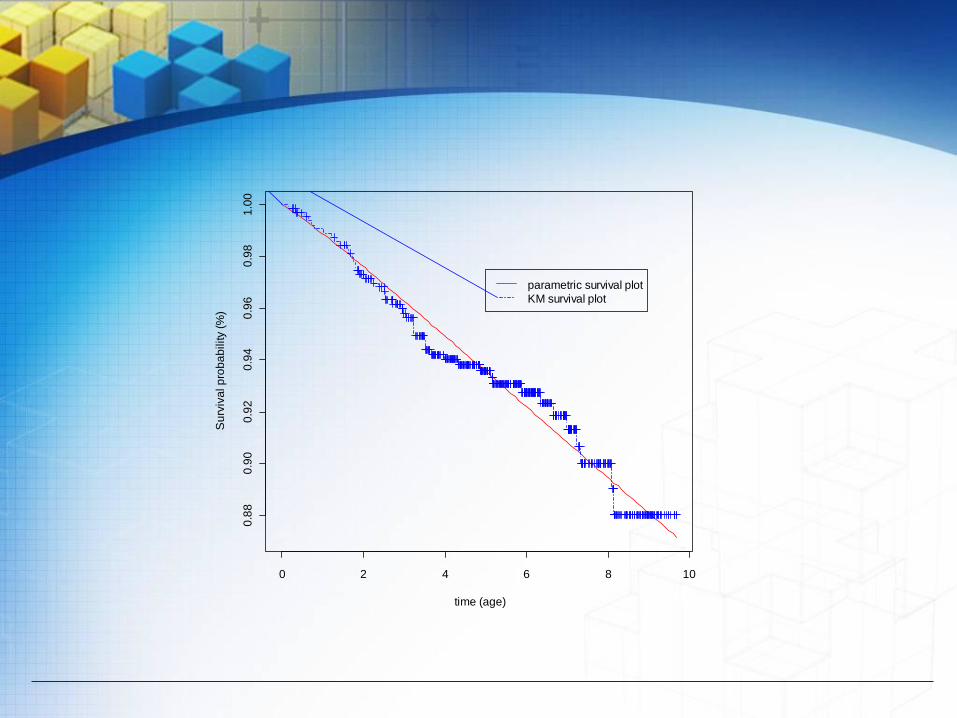
The survival probability estimate of the censored data using the KM model with the parametric survival model is given by Figure 4.1, below. In comparing the KM survival curve with the parametric model using the probability residuals, we have found that the mean of the probability residual is 0.000495, sample variance is 4.596*10^(-5), sample standard deviation is 0.0068 and standard error is 0.0024.
0 2 4 6 8 10
0.8
80
.90
0.9
20
.94
0.9
60
.98
1.0
0
time (age)
Su
rviv
al p
rob
ab
ility (
%)
parametric survival plot
KM survival plot

Cox PH Model
To select the best possible Cox PH model for censored data, we consider the model has all terms significant with the minimum AIC. Through statistical testing we have found that six first order terms and two interactions significantly contribute to the response variable. These attributable variables are tx, pathsize,nodediss, age, hrlevel, stnum, tx:age and nodediss:hrlevel. Thus, for the subject data and the attributable variables using the Cox PH model we plot the probability survival curve with the parametric survival curve and they are shown by Figure 4.2, below. In comparing the Cox PH curve with the estimated parametric survival curve, we found the mean of the probability residual is 0.028, sample variance is 0.000347, sample standard deviation is 0.0186 and standard error is 0.0066.

0 2 4 6 8
0.9
00
.92
0.9
40
.96
0.9
81
.00
time (age)
Su
rviv
al p
rob
ab
ility (
%)
parametric survival plot
Cox PH survival plot

KD survival analysis
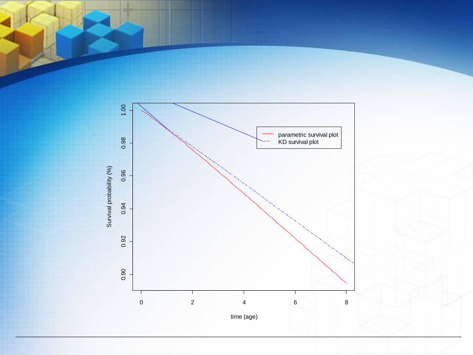
Despite the difficulties in working with censored data, we proceeded to use the nonparametric KD procedure to estimate the survival curve together with the fitted parametric survival curve. The results are shown by Figure 4.3, which are different than what we have found using KM and Cox PH models in terms of the smoothness of the curve.
In comparing the KD survival curve with the fitted parametric model, we have found the mean of the probability residual is 0.00883, sample variance is 2.942*10^(-5), sample standard deviation is 0.0054 and standard error is 0.00191.
Table 4.1, below, summarizes the response of the three survival analysis models, KM, Cox PH and KD, in comparison with the parametric model using the two parameter Weibull probability density function to characterize the failures. Thus, if we assume that we can proceed to statistically analyze the censored data, all three survival models performed well, but the edge goes to the KD model in terms of the smaller sample variance and standard error.
0 2 4 6 8
0.9
00
.92
0.9
40
.96
0.9
81
.00
time (age)
Su
rviv
al p
rob
ab
ility (
%)
parametric survival plot
KD survival plot

Residual analysis
Methods Mean SD SE Rank of model
Cox PH vs fitted parametric 0.028 0.0186 0.00658 3
Kaplan-Meier vs fitted parametric 0.000495 0.00678 0.002397 2
Kernel density vs fitted parametric 0.00883 0.0054 0.00191 1

CONCLUSIONS
The present study consists of three parts in comparing the effectiveness of three survival analysis models, namely, KM, Cox PH and KD.
Initially, using Monte Carlo simulation we compare the subject models with parametric survival models and found that the proposed KD survival model gives as good results, if not better, than the KM.
The second part consists of using actual uncensored breast cancer data. Performing a similar evaluation, the results support that the proposed KD model gives results in better estimates than the popular KM and Cox PH models with interactions.
Thirdly, we performed the same analysis with actual censored breast cancer data. Although working with censored data is quite difficult to justify such an analysis, under the circumstances we analyzed the data and the results are similar to the Monte Carlo simulation and using the uncensored data.

Part 2
IDENTIFY ATTRIBUTABLE VARIABLES AND INTERACTIONS IN BREAST CANCER
Statistical research team
Department of Mathematics and StatisticsUniversity of South Florida

The object of the present study is to develop a statistical model for breast cancer tumor size prediction for United States patients based on real uncensored data. We accomplish the objective by developing a high quality statistical model that identifies the significant attributable variables and interactions. We rank these contributing entities according to their percentage contribution to breast cancer tumor growth. This proposed statistical model can also be used to conduct surface response analysis to identify the necessary restrictions on the significant attributable variables and their interactions to minimize the size of the breast tumor. One can also use the proposed model to generate various scenarios of the tumor size as a function of different values of the subjective entities.
www.themegallery.com Company Logo

INTRODUCTION
The proposed model that we are developing includes individual variables, interactions, and higher order variables if applicable. In developing the statistical model, the response variable is the tumor size at diagnosis for breast cancer patients. We have identified 26 possible attributable variables for breast cancer, denoted, X1, X2,..., X26. For example, X1 stands for patient ID and X2 stands for the patient’s age at diagnosis. The list of attributable variables is in Table 1.1, below. In this study, we would like to find the relation between the tumor size and all other attributable variables. We cannot use survival time to predict the tumor size since death time happens after the tumor is detected. Therefore, we exclude the variable survival time(x25) and the censoring indicator function vss (x26) in the first part of study. Thus, we have only 24 variables left to construct our statistical model.

INTRODUCTION
In the present analysis, we used real data from the Surveillance Epidemiology and End Results (SEER) Program. SEER collects and compiles information on incidence, survival, and prevalence from specific geographic areas representing about 26 percent of the U.S. population plus cancer mortality for the entire U.S. [18].
The proposed statistical model is useful in predicting the tumor size given data for the attributable variables. It is statistically evaluated using R square, R square adjusted, the PRESS statistic and several types of residual analyses. Finally, its usefulness is illustrated by utilizing different combinations of the attributable variables.
In addition, the attributable variables are ranked according to their contributions to accurately estimate a patient’s tumor size.

HISTORICAL REVIEW
Survival analysis is used more and more in many areas. Many researchers have contributed to this subject. C. A. McGilchrist, [3], [4] discussed the regression with frailty in survival analysis. D. R. Cox, [7], [8] introduced the Cox proportional hazards (PH) model for survival data. E. L. Kaplan and P. Meier, [10] constructed Kaplan Meier empirical type of survival model. E. A. Gehan developed the generalized Wilcoxon test and this test is more powerful than the Cox proportional hazard’s test when the proportional hazard assumption is violated early on. K. Liu and C. P. Tsokos, [12], [13], [14] utilized kernel density methods in reliability analysis. N. Mantel and W. Haenszel, [16] proposed the Mantel Haenszel test for survival analysis. P. Qiu and C. P. Tsokos studied extensively the accelerated life testing model. Y. Xu and C. P. Tsokos, [20] probabilistically discussed and evaluated several most commonly used survival analysis models.
Some classical historical research papers can be found in [1], [6], [11] and [17]. Other important and recent references for the readers who will have an interest in survival analysis may be found in [5], and [15].

List of attributable variables
Name Full name of variables Short form
X1 Patient ID id
X2 Age at diagnosis age
X3 Year of Birth birthy
X4 Birth Place birthp
X5 Sequence Number Central snc
X6 Month of diagnosis month
X7 Year of diagnosis year
X8 Primary Site ps
X9 Laterality la
X10 Histologic Type ICDO3 ht
X11 Behavior Code ICDO3 bc
X12 Type of Reporting Source trs

List of attributable variables
X13 RXSumm SurgPrimSite rxps
X14 RXSumm Radiation rxr
X15 RXSumm RadtoCNS rxcns
X16 Age Recode Year olds ager
X17 Site Recode sr
X18 CSS chema css
X19 AJCC stage3 rdedition ajcc
X20 First malignant primary
indicator
findi
X21 State-county recode scr
X22 Race race
X23 Cause of Death to SEER
site recode
cod
X24 Sex sex
X25 Survival time recode survtime
X26 Vital Status recode vss

Breast Cancer Data Tree Diagram

We proceed to develop a statistical model taking into consideration the twenty four attributable variables listed in Figure above. The form of the statistical model is given by tumor size as a function of (x1, x2,… , x24). Note that some of the variables’ values are obtained after the tumor size is recorded. In our analysis all the patients in the data base have breast cancer. We utilize the values of the tumor size once the patient has gone through a diagnostic process. Thus, the general statistical form of the proposed model with all possible attributable variables and interactions will be of the form in equation below
jjii BBBAAATS ...... 221122110

One of the basic underlying assumptions in formulating an estimate of the above statistical model is that the response variable should be Gaussian distributed. Unfortunately, in the present form that is not the case. This fact is clearly demonstrated by the QQ plot shown by Figure below.

-2 -1 0 1 2
050
100
150
200
Normal Q-Q Plot
Theoretical Quantiles
Sam
ple
Qua
ntile
s

Furthermore, the Shapiro-Wilk normality test with the necessary calculation of the test statistic W = 0.7437 and p-value = 3.787e-15 is additional evidence that the tumor size does not follow normal probability distribution. We proceed in utilizing the Box-Cox transformation to the tumor size to determine if such a filter will modify the given data to follow the normal distribution so that we can proceed to formulate the proposed statistical model. Applying the Box-Cox transformation results in the statistical information presented in Table 3.1. One tumor size data’s value is zero and Box-Cox transformation can only apply to a positive data set. Therefore, we use .00000000000001 to replace this zero value so we can perform Box-Cox transformation.

Box-Cox Transformation for Normality for the Original Data
Box-Cox Transformation for Normality from Transformed Data
Est.Power Std.Err. Wald(Power=0) Wald(Power=1)
0.2659 0.0339 7.8445 -21.6563
Est.Power Std.Err. Wald(Power=0) Wald(Power=1)
1 0.1275 7.8444 -2e-04

-2 -1 0 1 2
01
23
4Normal Q-Q Plot
Theoretical Quantiles
Sa
mp
le Q
ua
ntil
es

During our statistical analysis in the estimation process, we found only four of the twenty-four attributable variables were significant contributors. We found only three higher order interactions to significantly contribute. The significantly contributing and interaction variables are RXR(X14), COD(X23), RXPS(X13) and AJCC(X19). However, SNC(X5), HT(X10), themselves individually do not significantly contribute to the response variables but when they interact with other variables they do significantly contribute to the response variable. Therefore, we still keep them in our final model. There are thirty-one missing values in the variable AJCC. We use the mean of the rest of the data value in the variable AJCC to replace the NA value in order to perform prediction of the model. Thus, the results of estimation of equation before are given by equation below as follows
19145
1-
14105
4-
191423
6-
19
3-
1413
-3
10
-4
5
-2.2659
10.191
10.91124. 1093.4102.72
3.3-10.28310.142102.09-7.2)ˆln(
XXX
XXXXXXX
XXXXST

List of Attributable Variables
NoIndividual
variablesName of individual variables
1 X5 Sequence Number Central
2 X10 Histologic Type ICDO3
3 X13 RXSumm SurgPrimSite
4 X14 RXSumm Radiation
5 X19 AJCC stage3 rdedition
6 X23 Cause of Death to SEER site recode
Interactions
7 X14:X19 RXR ∩ AJCC
8 X5:X10:X14 SNC ∩ HT ∩ RXR
9 X5:X14:X19 SNC∩ RXR ∩ AJCC
For our final model the R squared is 0.889 and R squared adjusted is 0.881. Both R squared value and R squared adjusted value are high (close to 90%) and these two are very close to each other. This shows our model’s R squared increase is not due to the increase of the parameters’ estimates, but rather the good quality of the proposed model to predict tumor size given values of the identified attributable variables [2]. Secondly, the PRESS statistics’ results support the fact that the proposed model is of high quality. We list in Table 3.3 the best three models based on the PRESS statistic out of total thirty-six models. From that table it is clear that the best model is number 36, which is our final model.
Furthermore, R square and R square adjusted are calculated for those 36 models which are of interest but the proposed model still gives the best possible estimates of the tumor size for breast cancer in SEER’s data.
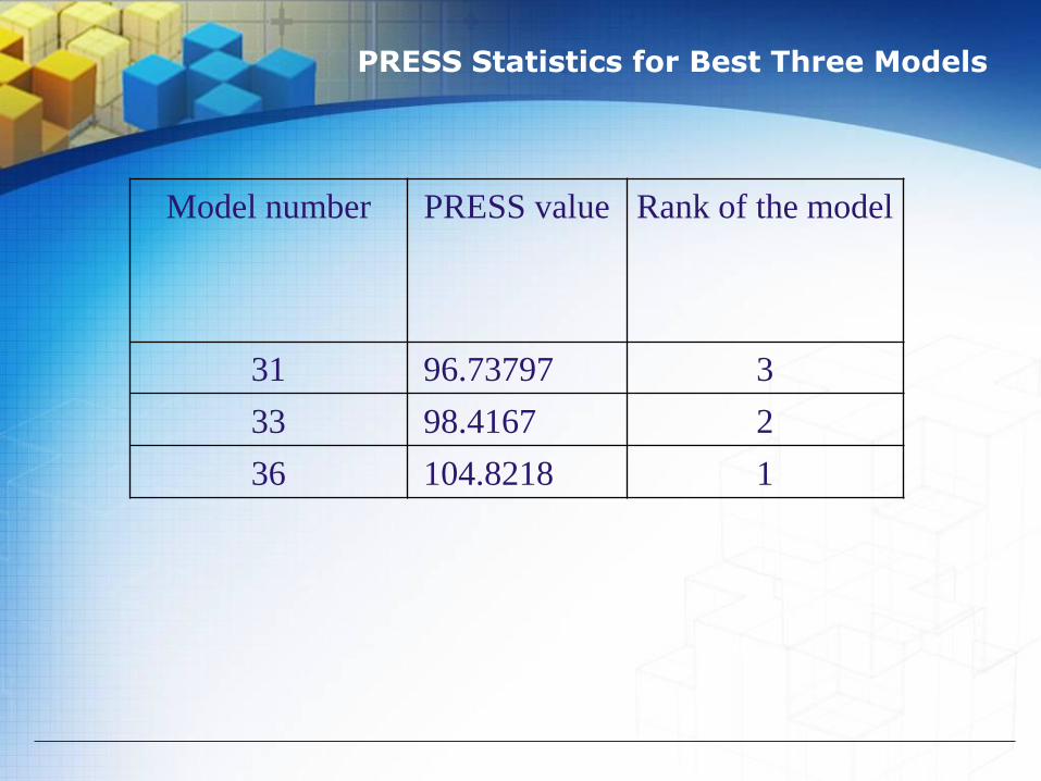
PRESS Statistics for Best Three Models
Model number PRESS value Rank of the model
31 96.73797 3
33 98.4167 2
36 104.8218 1

Breast Cancer Attributable Variable Diagram

Rank of Variable According to Contributions
Rank Variables
1 X5:X14:X19
2 X14:X19
3 X19
4 X5:X10:X14
5 X5
6 X14
7 X13
8 X10
9 X23

Residual Analysis
No Residual Values
146 1.3264266
147 1.0579828
148 0.9756659
149 1.7362950
150 0.9643773
151 1.2427113
152 1.3705402
153 1.3640997
154 1.6072370
155 1.9573079

We first randomly divide the data into two datasets of the same size. We use one of the datasets to construct the model and then use the resulting model to predict the values in the other dataset. Then we will switch the two data sets and repeat the procedure. The mean of all residuals turned out to be 1.0652916.
Next, we divided the dataset into six small data sets and use five of them to construct the model and validate the model using the sixth one. We will repeat the same procedure for each of the six small datasets. The mean of all residuals was 0.1318486.
Finally, we divided the dataset into 155 datasets and use all 154 datasets to construct the model and validate the model using the one left out. We repeat the procedure 155 times. Table 4.2 shows the last ten residuals out of the total one hundred fifty-five residuals.
The mean of the residuals was 0.634, the variance of the residuals was 42.89, standard deviation of the residuals was 6.55 and standard error of the residuals was 0.53.

Residual Analysis for Cross Validation
No Residual Values
146 0.13328523
147 0.08479963
148 0.07219656
149 0.36801567
150 0.07578824
151 0.11712640
152 0.14230504
153 0.14117093
154 0.19570259
155 0.29023850

USEFULNESS OF THE PROPOSED STATISTICAL MODEL
We can conclude from our extensive statistical analysis that there are only four significant attributable variables to the tumor size for breast cancer namely, RXR(X14), COD(X23), RXPS(X13) and AJCC(X19). As for SNC(X5), HT(X10). They themselves individually do not significantly contribute to the response variables; however, when they interact with other variables, they do significantly contribute to the response variable. Furthermore, we also tested two thousand and three hundred possible interactions of the attributable variables and we found three interactions to significantly contribute to tumor size for breast cancer.

USEFULNESS OF THE PROPOSED STATISTICAL MODEL
This model is useful for a number of reasons.
1. It can be used to identify the significant attributable variables.
2. It identifies the significant interactions of these attributable variables.
3. The most significant contributions to the tumor size growth are ranked.
4. One can also use the proposed model to generate various scenarios of the tumor size as a function of different values of the subjective entities.
5. A confidence interval for the tumor size can be constructed with parametric analysis. By obtaining the % confidence limits for the response, we can describe how confident we are that our estimate is close to the actual tumor size.
6.The model as shown in equation (3.3) can be used to perform surface response analysis to place the restrictions on the significant attributable variables and interactions to minimize the breast cancer tumor size. We can also put restrictions on the variables to minimize the response of the tumor size by nonlinear control with % confidence limits.

CONCLUSIONS & DISCUSSION
In the present study, we performed parametric analysis to estimate tumor size for breast cancer patients. The initial measurement of tumor size was collected from the SEER database. Those data do not follow normal probability distribution. Using the standard Box-Cox transformation, the SEER tumor size data became approximately normally distributed. We developed a “nonlinear” statistical model (nonlinear in terms of the power and logarithm of the response variable). Through the process of developing the statistical model, we found only four variables, namely, rxr(X14), cod(X23), rxps(X13) and ajcc(X19) and three interactions that significantly contribute to the tumor size. The proposed statistical model was evaluated using the R-square, R-square adjusted, PRESS statistics and three cross validation methods, all of which support the high quality of the developed statistical model. This model can be used to obtain a good estimate of tumor size knowing the four significantly attributable variables and three interaction terms.

LOGO
Statistical modeling of breast cancer using differential equations
Statistical research team
Department of Mathematics and StatisticsUniversity of South Florida
Part 3

The object of the present study is to utilize the attributable variables and interactions that have been identified to cause the breast tumor (cancer) to develop a differential equation that will characterize the behavior of the tumor as a function of time. Having such a differential equation, the solution of which once plotted will identify the rate of change of tumor size as we increase time (age). Once we have the differential equations and the solution of the differential equation, we can validate the quality of the proposed differential equations.

How do we determine the partition of the age?
In order to make the differential equation to maximize the quality of the model. Since the tumor growth rate is vary according to age. We will truncate the data starting from age 40 to age 85. Because we for patients who’s age is from 33 to 37 and age 39 we have missing data. For people who’s age is more than 85, the cause of death can be more complicated. Even the natural death can be more chances, therefore we decide to truncated the data from age 40 to age 85. We want our differential equations to be connect in all intervals therefore we will use same connection point for two adjacent intervals.

Breast Cancer Tree Diagram
814 patients’
data with
available
information
Original 1000
patient data
First age group
is patients from
age 40 to 58
Second age group
is patients from
age 58 to 70
1
3
Total 159 patients
with minimum size
of tumor is 0 mm
and maximum size
of tumor is 120 mm
Total 81 patients with
minimum size of
tumor is 1 mm and
maximum size of
tumor is 140 mm
Minimum age is 32 and
maximum age is 101
Minimum size of tumor
is 0 mm and maximum
size of tumor is 200 mm
Total 226 patients with
minimum size of
tumor is 1 mm and
maximum size of
tumor is 200 mm
Third age group is
patients from age
70 to 73
2
4
Forth age group
is patients from
age 73 to 85
Total 397 patients
with minimum size
of tumor is 0 mm
and maximum size
of tumor is 140 mm

For age from 40 to 58
40 45 50 55
1020
3040
x5
z5

Let X stands for the term of years and the instantaneous change of rate is: TS stands for tumor size.
The differential equation is
6452432
2456
10685.210773.7345.91097.5
1014.210076.410224.3TSTS
xxxx
xx
,

From this DF we can know the relationship between the size of tumor and the derivative of the tumor size.
The solution to the above DF is integratable DF as follow:
Multiple R-squared: 0.773, Adjusted R-squared: 0.6595
534
32345
10611.13967.
968.381091.110662.410542.4d(x)
d(TS)
xx
xxx

For age from 58 to 70
58 60 62 64 66 68 70
1520
2530
35
x5
z5

The differential equation is
From this DF we can know the relationship between the size of tumor and the derivative of the tumor size.
The solution to the above DF is integratable DF as follow:
Multiple R-squared: 0.8515, Adjusted R-squared: 0.7773
4232
2245
10908.21039.7
10031.710968.2106887.4TSTS
xx
xx
,
3234116.518.22104512.110113.3
d(x)
d(TS)xxx
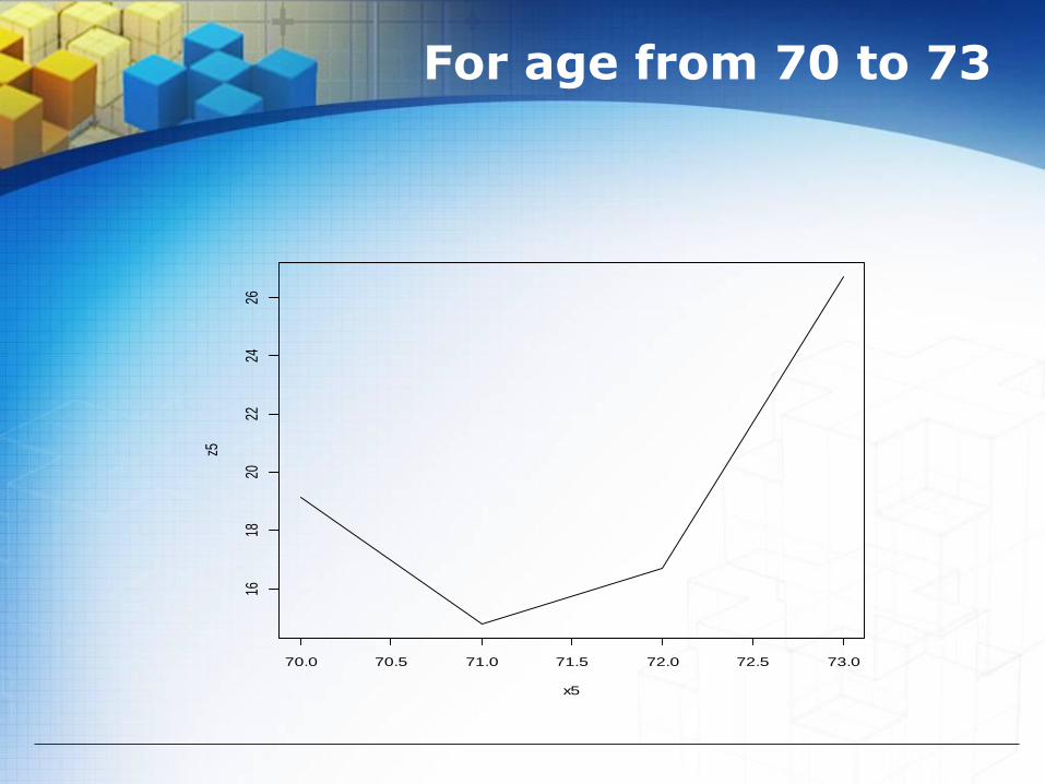
For age from 70 to 73
70.0 70.5 71.0 71.5 72.0 72.5 73.0
1618
2022
2426
x5
z5

The differential equation is
The solution to the above DF is integratable DF as follow:
Multiple R-squared: 0.9998, Adjusted R-squared: 0.9994
221816.857.2510231.9TSTS xx
,
x3632.857.25d(x)
d(TS)

For age from 73 to 85
74 76 78 80 82 84
1618
2022
2426
x5
z5

The differential equation is
The solution to the above DF is integratable DF as follow:
Multiple R-squared: 0.9805, Adjusted R-squared: 0.9665
53432
2457
10474.47506.110737.2
1014.210347.8103.1TSTS
xxx
xx
,
42
32245
10237.2
092.710424.810446.410792.8d(x)
d(TS)
x
xxx

LOGO
Part 4POWER LAW PROCESS IN CANCER ANALYSIS
Statistical research team
Department of Mathematics and Statistics
University of South Florida

ABSTRACT
The object of the present study is to propose the power law
process also known as non homogenous poison process which is
identical to the weibull process in analyzing and modeling
different types of cancer, especially breast cancer.
The key objective is to study the change of the tumor growth as a
function of age. The intensity function within the power law
process will give us the rate of change of the tumor growth as a
function of time.
In addition the key parameter within the intensity function can
give us the preliminary indication of the behavior of the tumor
subject to a given treatment.

POWER LAW PROCESS ANALYSIS
Power law process (PLP) also named non-homogeneous poisson process (NHPP) as well as weibull process (WP). [4]. PLP has been used in many applications. PLP is a special Poisson process and Poisson process is one of counting process.
A counting process is a stochastic process that possesses the following properties:
1. N(t) >0 2. N(t) is an integer. 3. If s<= t then N(s) <= N(t). If s< t, then N(t)-N(s) is the number of events
occurred during the interval (s,t] .[5]
,...1,0!
)(]))())([( ,
,
kk
ekaNbNP
k
baba

POWER LAW PROCESS ANALYSIS
NHPP has the intensity function:
V(t) has been very successfully used in reliability analysis v(t)=f(beta)
.0,0,0,)(
1
tfort
t

POWER LAW PROCESS ANALYSIS
We know that if the parameter beta is greater than one, then the tumor size increase means the survival rate decreased. If beta is less than one in survival analysis, then the tumor size decrease which means the survival time increase. If beta equals to one then the tumor size is constant and the NHPP will become homogenous passion process (HPP).
The unbiased estimator of beta is provided by bain and Enelhardt (1991). [8]
n
i i
n
MLEU
t
t
n
n
n
1
log
11ˆ

1) if the parameter beta is greater than one, then the tumor size increase means the survival rate decreased.
V(t)
t
2) If beta is less than one in survival analysis, then the tumor size decrease which means the survival time increase.
V(t)
t
3) If beta equals to one then the tumor size is constant and the NHPP will become homogenous passion process (HPP).
V(t)
t

POWER LAW PROCESS ANALYSIS
Gamma is indicator function. If gamma=1 the system will be failure time truncated, means our system is restricted by a number of tails and we will stop the testing when we reach that number of testing. If gamma=0 the system will be time truncated, means our system is restricted by a final failure time and we will stop the testing when we reach that time. [8]
ˆ
1ˆ
n
tn

50000 patient
data which
randomly
choose from
SEER data
Original SEER
data of 578134
patients with
breast cancer
49715 female
patients 285 male patients
b
29640
Ductal
patient
s
530
Medu
llary
patien
ts
We use simple random
sample (SRS) to select
this 50000 data from
original data set
6340
Lobular
patients
6272
patients
NA
4034 black patients 2985 Asian (other)
patients 42782 white patients
199 unknown
(unspecified) patients
2820
Ductal
patient
s
108
Medul
lary
patient
s
462
Lobular
patients
2314
Ductal
patient
s
34
Medul
lary
patient
s
299
Lobular
patients
644
patients
NA
338
patients
NA
6813
Stage 1
patients
5054
Stage 2
patients
a

a
6813
Stage 1
patients
4893
patients
alive
1920
patients
dead
426
patients
dead
because
of breast
cancer
1494
patients
dead
because
of other
reseason
250
patients
dead
without
radiation
treatment
164
patients
dead with
beam
radiation
treatment
12
patients
dead with
other
treatment
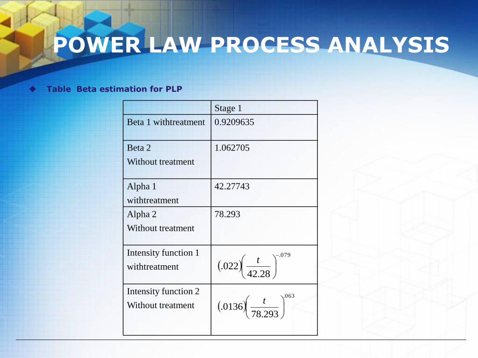
POWER LAW PROCESS ANALYSIS
Table Beta estimation for PLP
Stage 1
Beta 1 withtreatment 0.9209635
Beta 2
Without treatment
1.062705
Alpha 1
withtreatment
42.27743
Alpha 2
Without treatment
78.293
Intensity function 1
withtreatment
Intensity function 2
Without treatment
079.
28.42022.
t
063.
293.780136.
t

Intensity function with treatment
0 500 1000 1500 2000 2500
0.0
16
0.0
18
0.0
20
0.0
22
years
inte
nsity

Intensity function without treatment
0 500 1000 1500 2000 2500
0.0
13
0.0
14
0.0
15
0.0
16
0.0
17
years
inte
nsity

CONCLUSIONS & DISCUSSION
We construct PLP for 1st stages of breast cancer patients. We calculated the beta for those PLP and found them all less than one. It is an indicator that the treatment works for those patients.
Future work We will continue do the study for more data and
eventually we can construct PLP for each stage, each tumor size available for all treatment and compare the results. Then we can make suggestion for patients with particular tumor size that which treatment is best for them to have maximum survival expectation. We will fix grade and behavior code with same sex, stage and tumor size.
We will expand this form uncensored case to censored case.
We can also apply PLP in Bayesian survival analysis to improve our result and give better suggestions.

REFERENCES
A. W. Fyles, D. R. McCready, L. A Manchul., M. E. Trudeau, P. Merante, M. Pintile, L. M. Weir, and I. A. Olivotto, Tamoxifen with or without breast irradiation in women 50 years of age or older with early breast cancer, New England Journal of Medicine, 351 (2004) 963-970.
B. Abraham and J. Ledolter, Introduction to regression modeling, 2006 C. A. McGilchrist and C.W. Aisbett. Regression with Frailty in Survival
Analysis. Biometrics, 47(2):461-466, 1991. C. A. McGilchrist, REML Estimation for Survival Models with Fraility.
Biometrics, 49(1):221-225,1993 D. Collett, Modeling survival data in medical research (Chapman &
Hall/CRC) , 2003. D. P. Harrington, T.R. Fleming, A Class of Rank Test Procedures for
Censored Survival Data. Biometrika, 69(3):553-566, 1982. D. R. Cox, Regression models and life-tables (with discussion). Journal of
the Royal Statistical Society Series B, 34: 187–220, 1972. D. R. Cox and D. Oakes, Analysis of survival data (London: Chapman &
Hall), 1984. E. L. Kaplan and P. Meier. Nonparametric estimation from incomplete
observations. 53:457-448, 1958. J. P. Klein. Semiparametric Estimation of Random Effects Using the Cox
Model Based on the EM Algorithm. Biometrics, 48(3)795-806, 1992.

REFERENCES
K. Liu and C. P. Tsokos, Nonparametric Density Estimation for the Sum of Two Independent RandomVariables, Journal of Stochastic Analysis, 2000
K. Liu and C. P. Tsokos, Nonparametric Reliability Modeling for Parallel Systems, Journal of StochasticAnalysis, 1999
K. Liu and C. P. Tsokos, Optimal Bandwidth Selection for a Nonparametric Estimate of the Cumulative Distribution Function‖, International Journal of Applied Mathematics, Vol.10, No.1, pp.33-49, 2002.
N. A Ibrahim, A. Kudus, I.Daud, and M. R. Abu Bakar, Decision tree for competing risks survival probability in breast cancer study, International Journal of Biomedical Sciences Volume 3 Number 1, 2008.
N. Mantel and W. Haenszel, Statical aspects of the analysis of data from retrospective studies of disease. Journal of the National cancer Institute, 22(4), 1959.
P. Qiu and C. P. Tsokos, Accelerated Life-Testing Model Building with Box-Cox Transformation, Sankhya, Vol. 62, Series A, Pt. 2, pp. 223-235, 2000.
U.S. National institutes of Health, http://seer.cancer.gov Wikipedia, http://en.wikipedia.org/wiki/Breast_cancer Y. Xu and C. P. Tsokos, Probabilistic Comparison of Survival Analysis
Models using Simulation and Cancer Data, Communications in Applied Analysis, 2009, accepted

LOGO