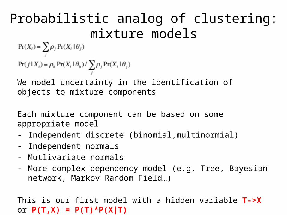
Probabilistic analog of clustering: mixture models

We model uncertainty in the identification of objects to mixture components

Each mixture component can be based on some appropriate model- Independent discrete (binomial,multinormial)- Independent normals- Mutlivariate normals- More complex dependency model (e.g. Tree, Bayesian network, Markov

Random Field…)

This is our first model with a hidden variable T->X or P(T,X) = P(T)*P(X|T)The probability of the data is derived by marginalization over the hidden variables

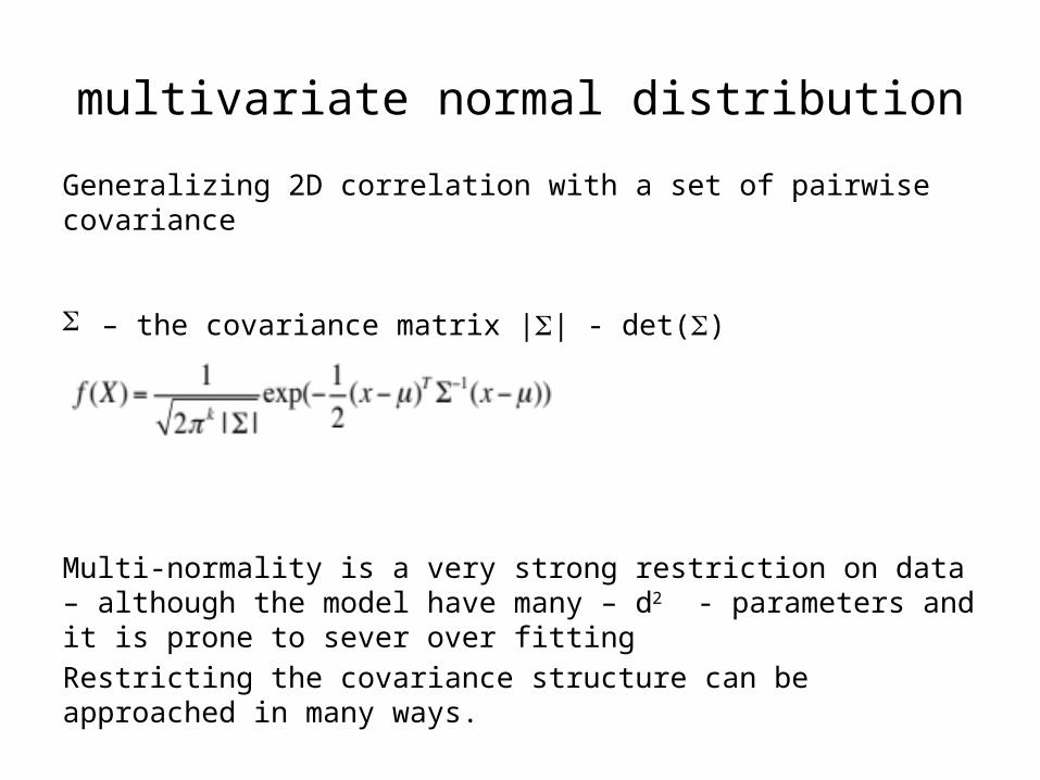
multivariate normal distribution

Generalizing 2D correlation with a set of pairwise covariance

S – the covariance matrix |S| - det(S)

Multi-normality is a very strong restriction on data – although the model have many – d2 - parameters and it is prone to sever over fittingRestricting the covariance structure can be approached in many ways.

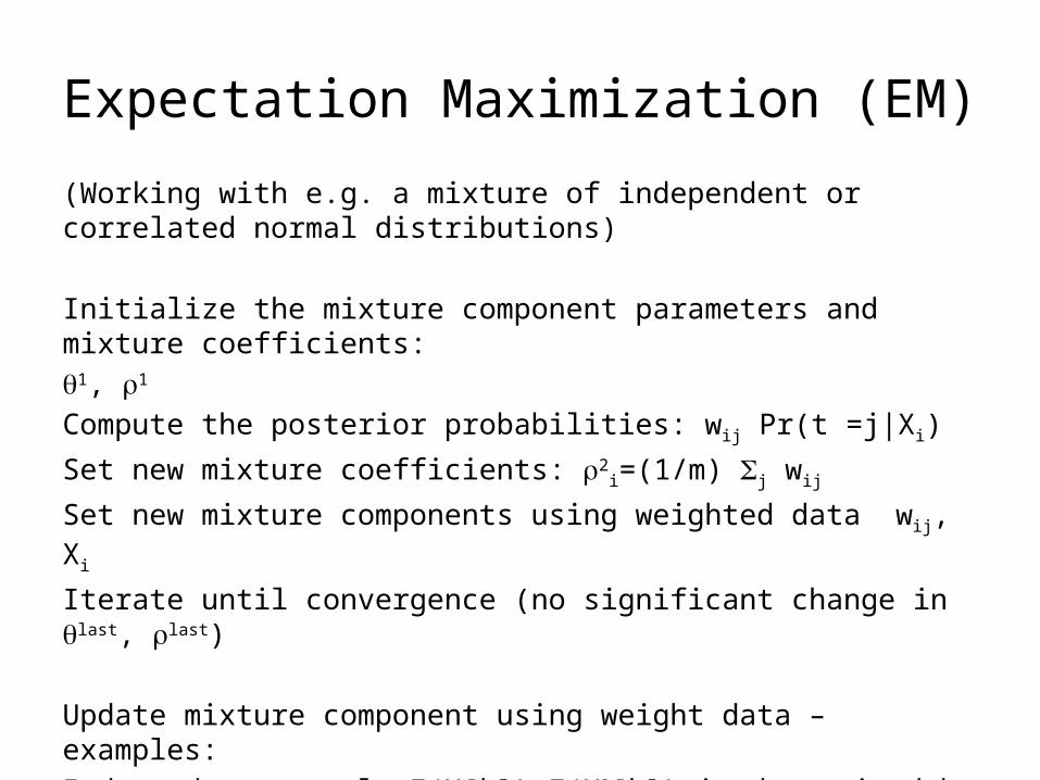
Expectation Maximization (EM)(Working with e.g. a mixture of independent or correlated normal distributions)

Initialize the mixture component parameters and mixture coefficients:q1, r1

Compute the posterior probabilities: wij Pr(t =j|Xi)

Set new mixture coefficients: r2i=(1/m) Sj wij

Set new mixture components using weighted data wij, Xi

Iterate until convergence (no significant change in qlast, rlast)

Update mixture component using weight data – examples:Independent normal: E(X[k]) E(X2[k]) is determined by weighted statisticsFull multivariate: all statistics (E(X[k]X[u]) is determined by weighted stats

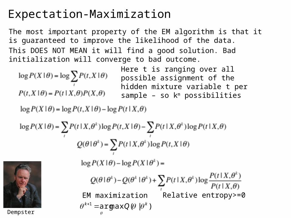
Expectation-Maximization

Relative entropy>=0EM maximization

)|(maxarg1 kk Q

Dempster

The most important property of the EM algorithm is that it is guaranteed to improve the likelihood of the data.This DOES NOT MEAN it will find a good solution. Bad initialization will converge to bad outcome.

Here t is ranging over all possible assignment of the hidden mixture variable t per sample – so km possibilities

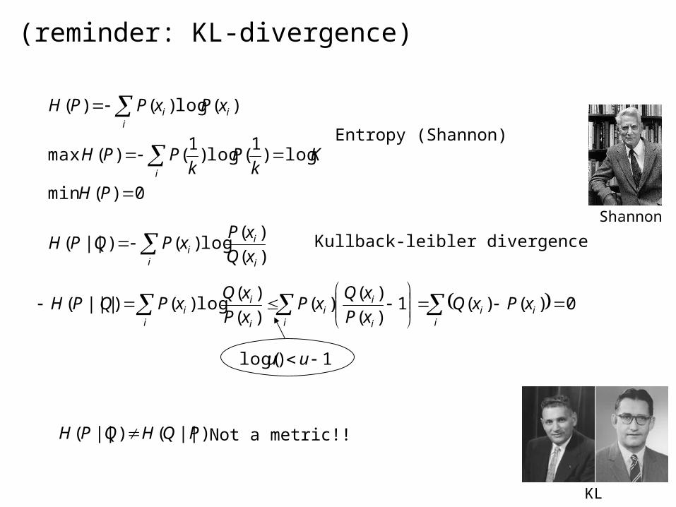
(reminder: KL-divergence)

0)(min

log)1(log)

1()(max

)(log)()(

PH

Kk

Pk

PPH

xPxPPH

i

iii

Entropy (Shannon)

i i

ii xQ

xPxPQPH

)(

)(log)()||( Kullback-leibler divergence

iii

i i

ii

i i

ii xPxQ

xP

xQxP

xP

xQxPQPH 0)()(1

)(

)()(

)(

)(log)()|||(

1)log( uu

)||()||( PQHQPH

KL

Shannon

Not a metric!!

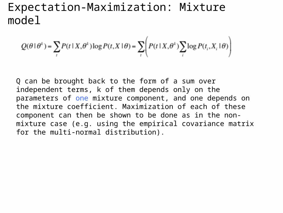
Expectation-Maximization: Mixture model

Q can be brought back to the form of a sum over independent terms, k of them depends only on the parameters of one mixture component, and one depends on the mixture coefficient. Maximization of each of these component can then be shown to be done as in the non-mixture case (e.g. using the empirical covariance matrix for the multi-normal distribution).

Multi-dimensional data: Analysis vs. modelingCases/experiments (n) X Features/Variables (m)Clustering one dimension to k behaviors: - km parameters using means only- km*2 parameters using mean/variance- K[m+m*(m-1)/2] full covariance matrix for each cluster..

Why modeling?- Further reducing the number of parameters- Extracting meaningful model parameters, features, dependency -> out ultimate

goal as analysts

What we are not going to do here:- Classification- Black box regressionAs analysts this is typically less attractive to us.It is by far more prone to experimental and other biases

Examples again (explained in class)

• Gene expression of single cells (cells/genes)Regulating genes predict regulated genes in cells(model within coherent cell populations)

• Patients/medical recordVarious clinical factors predict hypertension(model within coherent patient populations)

• User records in google (user/(search->ad->hit))User search phrase history predict response to add(Model within coherent user populations)

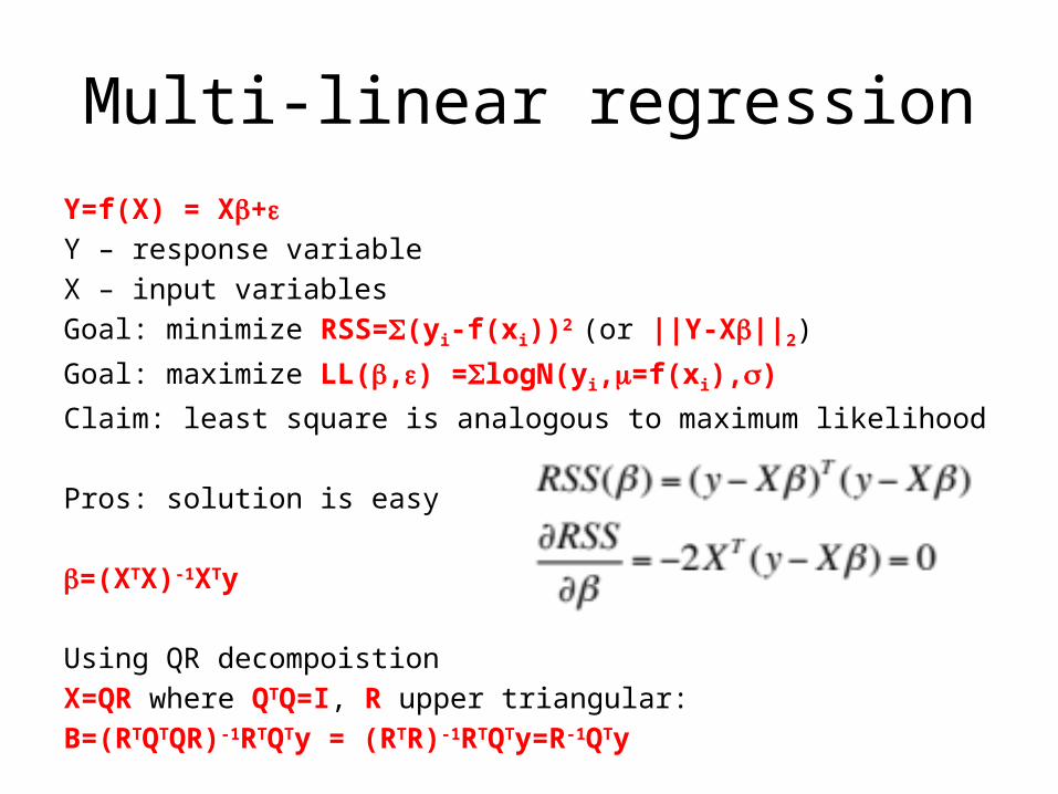
Multi-linear regressionY=f(X) = Xb+eY – response variable

X – input variables

Goal: minimize RSS=S(yi-f(xi))2 (or ||Y-Xb||2)

Goal: maximize LL(b,e) =SlogN(yi,m=f(xi),s)

Claim: least square is analogous to maximum likelihood

Pros: solution is easy

b=(XTX)-1XTy

Using QR decompoistion

X=QR where QTQ=I, R upper triangular:

B=(RTQTQR)-1RTQTy = (RTR)-1RTQTy=R-1QTy

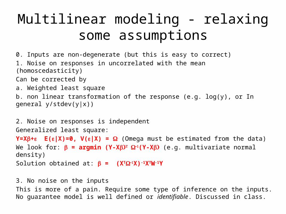
Multilinear modeling - relaxing some assumptions

0. Inputs are non-degenerate (but this is easy to correct)

1. Noise on responses in uncorrelated with the mean (homoscedasticity)

Can be corrected by

a. Weighted least square

b. non linear transformation of the response (e.g. log(y), or In general y/stdev(y|x))

2. Noise on responses is independent

Generalized least square:

Y=Xb+e E(e|X)=0, V(e|X) = W (Omega must be estimated from the data)

We look for: b = argmin (Y-X )b T W-1(Y-X )b (e.g. multivariate normal density)

Solution obtained at: b = (XTW-1X)-1XTW-1Y

3. No noise on the inputs

This is more of a pain. Require some type of inference on the inputs. No guarantee model is well defined or identifiable. Discussed in class.

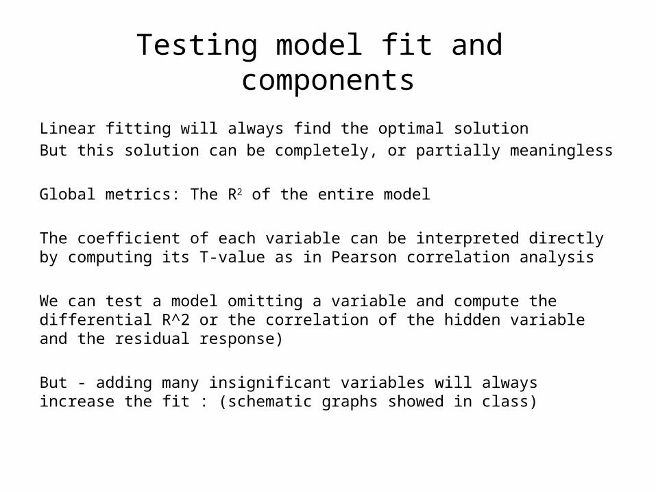
Testing model fit and components

Linear fitting will always find the optimal solutionBut this solution can be completely, or partially meaningless

Global metrics: The R2 of the entire model

The coefficient of each variable can be interpreted directly by computing its T-value as in Pearson correlation analysis

We can test a model omitting a variable and compute the differential R^2 or the correlation of the hidden variable and the residual response)

But - adding many insignificant variables will always increase the fit : (schematic graphs showed in class)

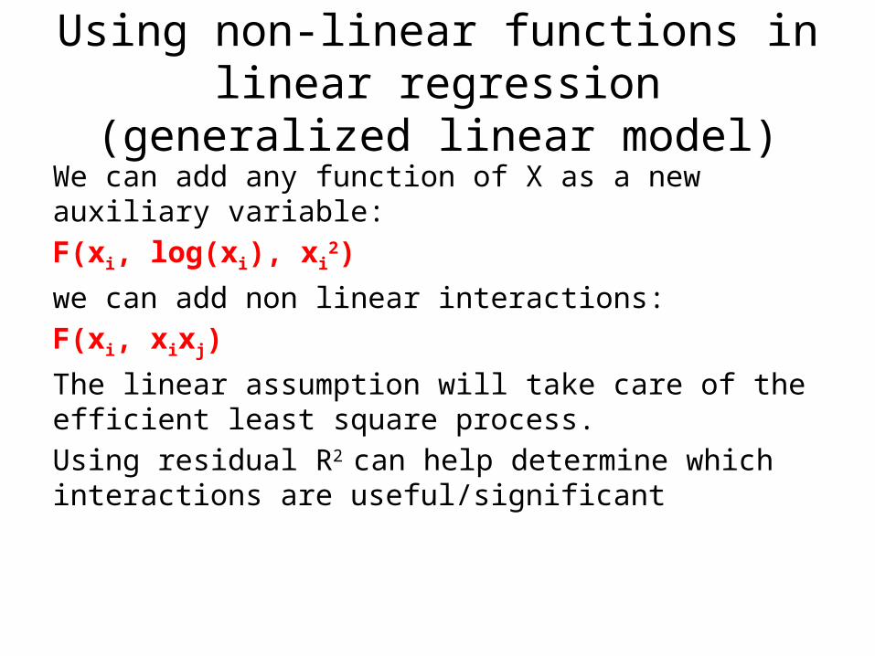
Using non-linear functions in linear regression (generalized linear model)

We can add any function of X as a new auxiliary variable:F(xi, log(xi), xi

2)

we can add non linear interactions:F(xi, xixj)

The linear assumption will take care of the efficient least square process. Using residual R2 can help determine which interactions are useful/significant

Testing subsets; Greedy approaches

Given a large number of potential input variables, we can try to find the best subset of variables such that all of them a residually significanta) Start from all the variables and eliminate iteratively the

worst variableb) Start from the highest correlation variable and iteratively

add the variable with highest correlation to the residualc) Do any local optimization (Adding and removing variables)

Cross validationA model with significant R2 can be achieved by pure chance given many candidate inputs and inadequate sample size

A robust procedure for controlling such over fitting is cross validation1. Divide the data into k partsFor each i:2. Fit the data while omitting the data in the ith part3. Compute the performance of the resulting model on the hidden dataThe resulting cross validation R^2 should be reasonably similar to the one obtained when working on all the data.You can draw a graph showing reduction in cross validation fit given various modeling decisions

In particular, when you divide a dataset of n cases into n parts the procedure is called leave-one-out cross validation.

Not covered here: Akaike information criterion (AIC), Bayesian information criterion (BIC) and other theoretically founded tools for model selection.

Ridge/Tikhonov regressionTo control over-fitting when using a large number input variables, we can add a regularization component to the regression goal function:||Y-Xb||2

+ ||Gb||2

When gamma equals aI (the unit matrix times alpha), this is called ridge regression, and set a fixed penalty on non-zero coefficients.Gamma can also encode smoothing constraints such as when using a difference operator. This is useful if the input variable are assumed to represent related effects.

Conveniently, the solution to the Tikhonov regression is still explicit:b=(XTX + GTG)-1XTy(in the case of ridge regression, we simply add a constant to the diagonal of XTX)Note the analogy of ridge regression and assuming a Bayesian normal prior centered on 0 on the coefficients (paying ||Gb||2 in log probability)

Lasso and Elastic net regression

Instead of Gaussian priors on the coefficient, we may wish to penalize coefficients linearly. This will give more weight to eliminating small coefficients, and will be less troubled by having few strong coefficients:||Y-Xb||2

+ l1||b||

In particular, we can solve the standard least square problem under the constraint of ||b||<t (a.k.a. the lasso). This is solved by quadratic programming (or convex optimization)

Shrinking the lasso and observing cross validation R^2 is routine.It is also possible to combine ridge and lasso, a method nicknamed elsatic net (this penalize very large coefficients, but also avoid many small coefficients):||Y-Xb||2

+ l1||b||+l2||b||2

Discrete and non parametric modelingY=f(x1,x2) – but the functional form is very unclear

On the other hand, there is a lot of data

We can discretize x1,x2 and study the table (y|bin1,bin2).(for example, y can be normally distributed within each bin).(or, y can be a linear function of x1,x2 in each bin)

This a-parametric approach lose power since each bin is treated independently. But if a dataset is extensive, this may not be a problem.It is not easily scalable to many inputs, unless some parametric assumptions can be used

Parametric non-linear fitting

Y=f(x;a) – any function we know how to differentiatec2= (S yi-yi(x;a))/si

Important: we know how to compute the gradient and hessian of the function

Minimization is done using a combination of gradient descent and solution to the local linear least square problem (Levenberg-Marquardt method)

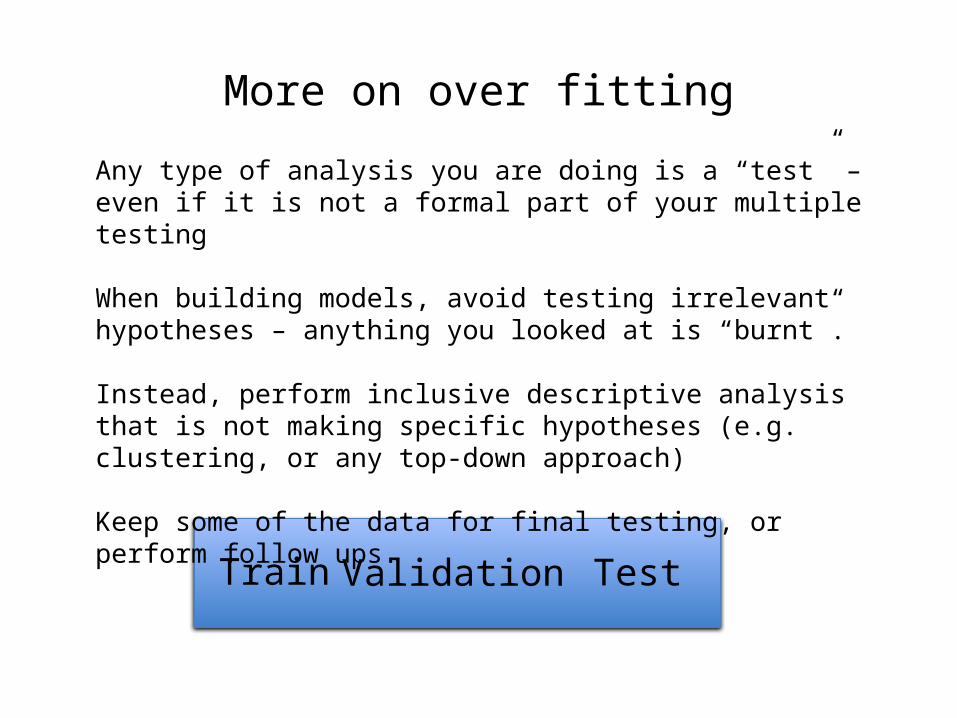
More on over fitting

Train Validation Test

Any type of analysis you are doing is a “test” – even if it is not a formal part of your multiple testing

When building models, avoid testing irrelevant hypotheses – anything you looked at is “burnt”.

Instead, perform inclusive descriptive analysis that is not making specific hypotheses (e.g. clustering, or any top-down approach)

Keep some of the data for final testing, or perform follow ups.

Accurate modeling does not imply causality

• A variable can predict other variables because of indirect, non causal relation

• A->B->C can be transformed to C->B->A(how? Compute!)• How can we infer causality: Perturbation/interventions (experiments) Time separation More?