PRICE MANIPULATION AND QUASI-ARBITRAGE1

BY GUR HUBERMAN AND WERNER STANZL

In an environment where trading volume affects security prices and where prices

are uncertain when trades are submitted, quasi-arbitrage is the availability of a series

of trades which generate inÞnite expected proÞts with an inÞnite Sharpe ratio. We

show that when the price impact of trades is permanent and time-independent,

only linear price-impact functions rule out quasi-arbitrage and thus support viable

market prices. When trades have also a temporary price impact, only the permanent

price impact must be linear while the temporary one can be of a more general form.

We also extend the analysis to a time-dependent framework.

KEYWORDS: Market microstructure, price impact, arbitrage, market viability,

gain-loss ratio.

1. INTRODUCTION

IN ANY MARKETS, trades can affect prices. In Þnancial markets, the same individual can buy

and subsequently sell the same security. In principle, then, a trader in a Þnancial market can

manipulate prices by buying and then selling the same security, with the expectation of earning

a positive proÞt from such a manipulation.

This paper takes the perspective of a market watcher who has no opinion on the direction

of security price movements but is an excellent student of the relation between trades and price

1

changes. In fact, he has estimated that relation and is tempted to exploit this knowledge to his

advantage. In a market in which prices are uncertain when orders are submitted, he attempts to

implement a quasi-arbitrage which is a trading strategy that produces inÞnite expected proÞts

with an inÞnite Sharpe ratio. What are the possible relations between price changes and trades

that rule out quasi-arbitrage for this market watcher?

The absence of quasi-arbitrage is tantamount to market viability. A market is viable if the

optimal demand of an agent with a mean/standard-deviation utility function exists. This result

resembles that of Dybvig and Ross (1987) for the classical pricing model. They show that the

absence of pure arbitrage is equivalent to the existence of an optimum for an agent who prefers

more to less.

The dependence of price on trade size has an immediate as well as a permanent component.

The price-impact function is the immediate price reaction to trading volume, including both

temporary and permanent effects. The price-update function is the permanent effect of trade

size on future prices. This papers main result is the characterization of the price-update

function under time independence. SpeciÞcally, price-update functions that admit no quasi-

arbitrage possibilities and thus ensure viable markets are linear in trade size.

Recent empirical papers assume in addition to time independence that the price-impact and

price-update functions are the same and suggest nonlinear price-update functions. Examples

include Hasbrouck (1991), Hausman et al. (1992), and Kempf and Korn (1999). Interpreted in

light of this work, these empirical results imply the feasibility of price manipulation.

Alternatively, our work calls into question either the time independence underlying much

of the empirical work or the identiÞcation of the price-impact with the price-update function.

(Holthausen et al. (1987), Gemmill (1996), or Keim and Madhavan (1996) make exactly the

2

distinction between temporary and permanent effects of trades on prices.)

Anticipating some of this papers results, Black (1995) imagines equilibrium exchanges where

only limit orders labeled by levels of urgency are traded, and informally argues that price

moves at each urgency level should be roughly proportional to order sizes to avoid arbitrage.

Presumably, he had in mind a time-independent framework where trades have a permanent

price impact only. This paper does not address limit orders, but provides a formal proof of

Blacks conjecture when only market orders are allowed.

The standard justiÞcation of a price-impact function in an environment with asymmetrically

informed agents is that information is impounded into prices through trades. Kyle (1985) is the

leading example. Such models assume linear price-impact functions for tractability. This paper

argues that linearity is justiÞed in an environment that rules out quasi-arbitrage. It thereby

selects which price-impact and price-update functions qualify for equilibrium.

The framework of this paper can also be used to evaluate Blacks (1995) conjecture that the

Kyle (1985) model allows price manipulation. We demonstrate that this is wrong. Underlying

these results is a characterizing condition of the absence of price manipulation which governs

how liquidity is allowed to vary over time. Furthermore, we prove that under certain conditions

the equilibrium price-impact functions in Kyle have to be linear when time between trades is

small.

The recent incomplete-markets, asset-pricing literature suggests to impose bounds on either

the Sharpe ratio (see Cochrane and Saa-Requejo (2000)) or the gain-loss ratio (see Bernardo and

Ledoit (2000)) to rule out good deals. These bounds are then used to calculate price bounds

for the assets in the economy. The framework of this paper can also embed such restrictions on

prices. All results derived here for the absence of quasi-arbitrage are qualitatively the same as

3

those for imposing no good deals with inÞnite gain-loss ratio.

Also, a simple corollary of our analysis is that ruling out price manipulation in a pure risk-

neutral world has the same implications for the shape of the price-impact and price-update

functions as the absence of quasi-arbitrage. A risk-neutral price manipulation embodies a

trading strategy that generates positive expected proÞts.

Allen and Gale (1992) examine risk-neutral price manipulation in the Glosten and Milgrom

(1985) framework. They construct equilibria in which uninformed agents proÞtably manipulate

the security price. This price manipulation does not erode the equilibrium because traders

are volume-constrained. Jarrow (1992) investigates whether a large trader, whose trades move

the price in an otherwise complete and continuous-time market, can make proÞts from price

manipulation. He gives several examples of pure arbitrage and states a sufficient condition that

precludes arbitrage. The setups and results of both papers differ substantially from ours.

The rest of the paper is organized as follows. Section 2 introduces the model and describes

the properties of prices. It also deÞnes price manipulation and quasi-arbitrage. Section 3 Þnds

necessary and sufficient conditions for both the absence of price manipulation and the absence

of quasi-arbitrage, when the price-impact and price-update functions are time-independent.

Section 4 investigates time-dependent price-impact and price-update functions and discusses

the Kyle (1985) model. Section 5 treats multi-asset price dynamics. Section 6 studies the

relationship between price impact and the gain-loss ratio, and Section 7 concludes. All proofs

are relegated to the Appendix.

2. PRICE MODEL AND MARKET CONDITIONS

The Þrst subsection describes the trading environment and how trades affect price changes.

4

The second takes the viewpoint of a trader and deÞnes price manipulation and quasi-arbitrage.

The third explains why ruling out quasi-arbitrage is necessary for market viability. The fourth

is more technical and lays out possible assumptions regarding the probability distribution of

security prices.

2.1. Price Impact and Dynamics

Consider a trader of a single asset over N periods in the time interval (0, 1]. (The multi-asset

case will be discussed in Section 5.) The asset can be bought or sold via market orders at times

n4N , 1 ≤ n ≤ N , where 4N ≡ 1/N . In each period n, the initial price of the asset is given by

the price quote pn,N . In the absence of uncertainty, the trader, who trades the quantity qn,N ,

has to pay a total of pn,Nqn,N with pn,N = pn,N+Pn,N(qn,N). The initial price for the next period

will be the quote pn+1,N = pn,N + Un,N(qn,N ). A positive (negative) qn,N indicates a purchase

(sale). The price-impact function Pn,N measures the immediate price reaction to the trade qn,N ,

including both the permanent and the temporary price impact, while the price-update function

Un,N describes only the trades permanent price impact. Hence, the temporary price impact is

the difference Pn,N − Un,N .

In every period competitive liquidity providers stand ready to Þll the order of the trader.

They set quotes and transaction prices. The price-impact and price-update functions represent

their price reaction to trade size. Since the price-impact functions include the permanent price

impact, any new information contained in an order is incorporated into the transaction price

instantaneously.

Price-impact and price-update functions may be the consequence of either asymmetric in-

formation (see Glosten and Milgrom (1985), Kyle (1985), or Easley and OHara (1987, 1992))

or inventory costs (e.g., Amihud and Mendelson (1980) and Ho and Stoll (1981)). We nei-

5

ther model here how beliefs about the fundamental value of the asset are formed, nor do we

postulate a speciÞc dynamic for the inventory of the liquidity providers. Rather, we assume

that we are given a certain set of price-impact and price-update functions that are already the

outcome of these processes. The market can be in an equilibrium or a disequilibrium; it only

has to meet the assumptions that we make here regarding the trading environment, but, other

than that, can be very general. In particular, the price-impact and price-update functions may

not only incorporate the fundamental value of the asset and inventory effects, but also other

exchange-speciÞc characteristics that affect prices and are sensitive to trading volume.

The trader does not possess superior information about the value of the asset, but can trade

any amount he wishes. Others, called the trading crowd, may also submit orders. Their trade

sizes are random, from the traders perspective. All orders are submitted simultaneously at the

end of each period. In addition, news that reveal value-relevant information arrive randomly.

To incorporate both types of uncertainty, the price process is augmented with stochastic terms

as follows.

After the most recent trades at time (n− 1)4N , the price change due to public news, εn,N ,

is revealed at the beginning of period n and the price is updated to pn,N , taking into account

both the last trades and the latest news. Since the next trades take place only at time n4N and

the trading crowd does not reveal its intended orders, the trader knows pn,N and εn,N before his

trade in period n, but not the net order size of the trading crowd denoted by ηn,N . Our setup

should best capture real trading activity: while it is unlikely that new information occurs at

the moment of submitting a trade, other traders order submissions not known to a trader are

likely to happen.

For simplicity, the price-impact and price-update functions, Pn,N and Un,N , are both assumed

6

to be Þnite and deterministic functions of the total trading volume qn,N +ηn,N only. Hence, the

structure outlined above gives rise to the following price dynamics:

(1) pn,N = pn−1,N + Un−1,N (qn−1,N + ηn−1,N) + εn,N ,

pn,N = pn,N + Pn,N(qn,N + ηn,N),

for 1 ≤ n ≤ N , p0,N > 0, where pn,N denotes the transaction price at time n4N . Recall that

the prices given by (1) are set by the liquidity providers.

All random variables in (1) are deÞned on the same probability space, (Ω,F ,P). Both,

the εn,N s and the ηn,N s are i.i.d. processes with zero expected values, and are independent of

each other. The information of the liquidity providers before orders have been submitted at

time n4N is represented by the sigma-algebra F (N)n4Nand includes the knowledge of pj,Nnj=1,

pj,Nn−1j=1 , qj,N + ηj,Nn−1j=1 , and εj,Nnj=1. The transaction price pn,N and the total volume

qn,N + ηn,N are known only after the trades and hence belong to F (N)(n+1)4N

. Thus, the liquidity

providers observe the total trading volume, but never know its decomposition. Such providers

resemble the market makers in Kyle (1985).

The trader, in contrast, knows in addition to F (N)n4N

his own orders qj,Nnj=1 and extracts the

past orders of the trading crowd ηj,Nn−1j=1 from qj,N+ηj,Nn−1j=1 , at time n4N . However, he can

compute ηn,N only after the trades have taken place in that period. Conditional expectations,

denoted by En,N , are with respect to the private information of the trader, G(N)n4N.

The roles of the trader and the trading crowd can be interpreted in two ways. Either one

thinks of the trader as being a large monopolistic trader and the trading crowd as being noise

traders, or one sees the trader as a representative agent who believes that others orders are

7

noise. The model is a stylized model of microstructure. In most Þnancial markets, participants

can trade continuously, whereas here (as in other microstructure models, such as Kyle (1985))

they trade via a series of equally spaced auctions. Actual order ßows or even signed order

ßows seem to violate the i.i.d. assumption assumed about the ηn,N s. (See, e.g., Hasbrouck

and Ho (1987), and Madhavan, Richardson and Rommans (1997).) To accommodate these

empirical regularities one may want to interpret the ηn,N s as the unexpected demand of the

trading crowd. This interpretation leaves the analysis intact and is consistent with the observed

empirical regularities.

The functions Pn,N and Un,N can integrate bid-ask spreads and the market depths associated

with these spreads. For example, suppose that at time n4N the bid and the ask prices are

pn,N ∓ sn/2 for up to Sn shares. In addition, assume that after the trade at time n4N the new

mid-point quote equals the average of the previous mid-point quote and the last transaction

price, plus εn+1,N . This situation can be modeled by setting Pn,N(q) = sn/2 if 0 < q ≤ Sn,

= −sn/2 if −Sn ≤ q < 0, = 0 if q = 0, and Un,N = Pn,N/2. What Pn,N and Un,N look like

for trades larger than Sn will depend on other features of the trading environment, such as the

liquidity of the limit-order book and the upstairs market (if they exist), the trading protocols,

and so on.

The trading interval (0, 1] represents a short-term time horizon such as a day or a week.

Here, the time between trades, 4N , is exogenously Þxed by the exchange before trading starts;

later sections also allow the traders to choose 4N . Fixed transactions costs are charged by

intermediaries: c(k) > 0 speciÞes the total Þxed costs of k trades.

All variables and functions depend on the number of trades available, N , or equivalently,

on the length of the inter-trading interval, 4N . The sensitivity of the price-impact and price-

8

update functions to trading volume may change when 4N decreases. Section 2.4 states the

pertinent assumptions.

The ranges of the traders order size, qn,N , and the crowds trading volume, ηn,N , are DM

and Dη, respectively. The domain of the price-impact and price-update functions, D, is thus

DM +Dη.

A relatively tractable special case of (1) is

(2) pn,N = αpn−1,N + (1− α)pn−1,N + εn,N ,

pn,N = pn,N + Pn,N(qn,N + ηn,N),

where α ∈ [0, 1]. The price dynamics (2) can be obtained by setting Un,N = (1 − α)Pn,N in

(1). The trader faces a price quote that is a convex combination of the previous quote and

the transaction price of the last trade. In this case, temporary and permanent price changes

are closely linked. This will allow the derivation of stronger conditions that are implied by the

absence of quasi-arbitrage or the absence of price manipulation. When α = 0, i.e., Un,N = Pn,N ,

then (2) simpliÞes to

(3) pn,N = pn−1,N + Un,N (qn,N + ηn,N) + εn,N ,

implying that the price change is a function of the current trades and randomness only, i.e., it

does not depend on history. Further, the transaction price at time n4N equals the price quote

at time (n+ 1)4N minus εn+1,N , and each trade has only a permanent impact on the security

price.

Observe that the Kyle (1985) model can be recovered from (3), by setting εn,N = 0 and

9

making the Un,N s linear functions. Thus, the price model in (1) generalizes Kyles model.

2.2. DeÞnition of Price Manipulation and Quasi-Arbitrage

What are reasonable prices for the market model introduced in the previous section? Equiv-

alently, what do reasonable price-impact and price-update functions look like? Usually, the

absence of arbitrage is invoked to Þnd the set of viable asset prices. If arbitrage were feasible

and scalable, agents would want to trade an inÞnite amount of shares over a Þnite time horizon

and thus would cause the market to collapse. Two crucial assumptions underlying the classical

arbitrage theory are that traders know the prices at which they can trade at any time, and that

investments can be scaled without affecting prices.

Since we relax both of these assumptions, imposing the absence of pure arbitrage is less

suitable here. First, if prices are unknown before the trades, pure arbitrages are hard to

implement. Prices may fall after a sell order has been submitted or rise after a buy order

has been announced; such adverse price movements make it difficult to avoid states in which

losses occur with positive probability. Second, the dependence of prices on trade sizes limits

the proÞtability of pure arbitrage. In this case, the existence of arbitrage does not necessarily

imply the breakdown of a market. Hence, to identify the prices which support a viable market,

we do not employ a no pure-arbitrage condition but use the concept of price manipulation and

quasi-arbitrage as deÞned and discussed next.

A sequence of trades q0,N ≡ qn,NNn=1 is a round-trip trade if the sum of all these trades is

zero, i.e.,PN

n=1 qn,N = 0. This sequence may contain zero trades and thus the actual number

of trades, T (q0,N), may be strictly less than N . The proÞt of a round-trip trade is given by

(4) π(q0,N ) ≡ −NXn=1

pn,Nqn,N − c(T (q0,N)).

10

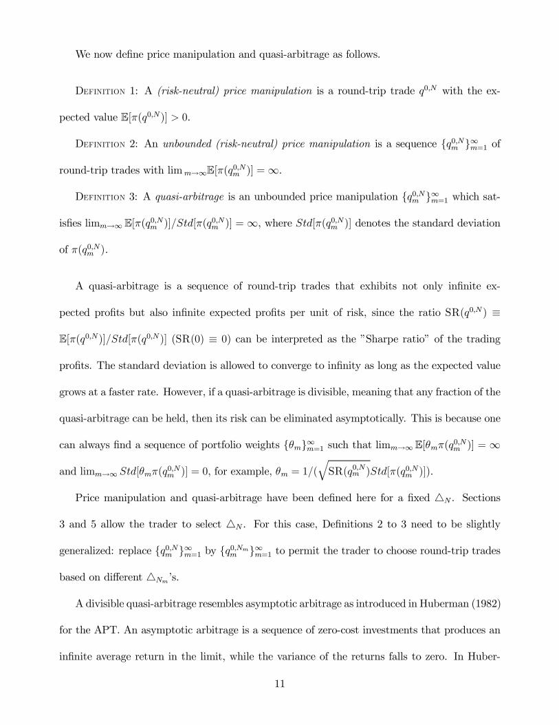
We now deÞne price manipulation and quasi-arbitrage as follows.

DEFINITION 1: A (risk-neutral) price manipulation is a round-trip trade q0,N with the ex-

pected value E[π(q0,N)] > 0.

DEFINITION 2: An unbounded (risk-neutral) price manipulation is a sequence q0,Nm ∞m=1 of

round-trip trades with limm→∞E[π(q0,Nm )] =∞.

DEFINITION 3: A quasi-arbitrage is an unbounded price manipulation q0,Nm ∞m=1 which sat-

isÞes limm→∞ E[π(q0,Nm )]/Std[π(q0,Nm )] =∞, where Std[π(q0,Nm )] denotes the standard deviation

of π(q0,Nm ).

A quasi-arbitrage is a sequence of round-trip trades that exhibits not only inÞnite ex-

pected proÞts but also inÞnite expected proÞts per unit of risk, since the ratio SR(q0,N ) ≡

E[π(q0,N)]/Std[π(q0,N )] (SR(0) ≡ 0) can be interpreted as the Sharpe ratio of the trading

proÞts. The standard deviation is allowed to converge to inÞnity as long as the expected value

grows at a faster rate. However, if a quasi-arbitrage is divisible, meaning that any fraction of the

quasi-arbitrage can be held, then its risk can be eliminated asymptotically. This is because one

can always Þnd a sequence of portfolio weights θm∞m=1 such that limm→∞E[θmπ(q0,Nm )] = ∞

and limm→∞ Std[θmπ(q0,Nm )] = 0, for example, θm = 1/(qSR(q0,Nm )Std[π(q0,Nm )]).

Price manipulation and quasi-arbitrage have been deÞned here for a Þxed 4N . Sections

3 and 5 allow the trader to select 4N . For this case, DeÞnitions 2 to 3 need to be slightly

generalized: replace q0,Nm ∞m=1 by q0,Nmm ∞m=1 to permit the trader to choose round-trip trades

based on different 4Nms.

A divisible quasi-arbitrage resembles asymptotic arbitrage as introduced in Huberman (1982)

for the APT. An asymptotic arbitrage is a sequence of zero-cost investments that produces an

inÞnite average return in the limit, while the variance of the returns falls to zero. In Huber-

11

man asymptotic arbitrage could occur when the number of assets becomes inÞnite; asymptotic

arbitrage here could occur when the trading volume goes to inÞnity.

Quasi-arbitrage is a weaker constraint than δ-arbitrage as introduced in Ledoit (1995).

Translated into this framework, a δ-arbitrage is a round-trip trade q0,N for which the Sharpe

ratio SR(q0,N ) is larger than δ. Obviously, the absence of δ-arbitrage excludes quasi-arbitrage.

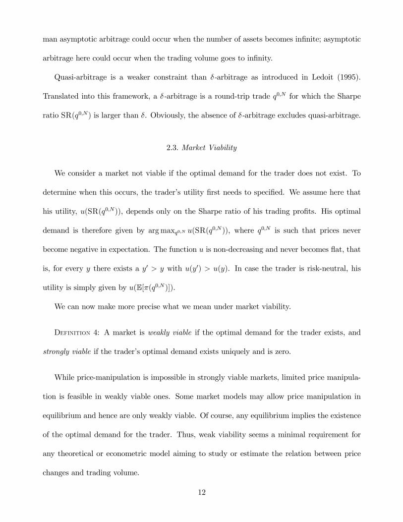
2.3. Market Viability

We consider a market not viable if the optimal demand for the trader does not exist. To

determine when this occurs, the traders utility Þrst needs to speciÞed. We assume here that

his utility, u(SR(q0,N)), depends only on the Sharpe ratio of his trading proÞts. His optimal

demand is therefore given by argmaxq0,N u(SR(q0,N )), where q0,N is such that prices never

become negative in expectation. The function u is non-decreasing and never becomes ßat, that

is, for every y there exists a y0 > y with u(y0) > u(y). In case the trader is risk-neutral, his

utility is simply given by u(E[π(q0,N )]).

We can now make more precise what we mean under market viability.

DEFINITION 4: A market is weakly viable if the optimal demand for the trader exists, and

strongly viable if the traders optimal demand exists uniquely and is zero.

While price-manipulation is impossible in strongly viable markets, limited price manipula-

tion is feasible in weakly viable ones. Some market models may allow price manipulation in

equilibrium and hence are only weakly viable. Of course, any equilibrium implies the existence

of the optimal demand for the trader. Thus, weak viability seems a minimal requirement for

any theoretical or econometric model aiming to study or estimate the relation between price

changes and trading volume.

12

Weak viability rules out quasi-arbitrage. This follows immediately from the assumptions on

u and the deÞnition of quasi-arbitrage. Whether the converse holds, is not obvious. We will

identify conditions under which the absence of quasi-arbitrage implies either strong or weak

viability.

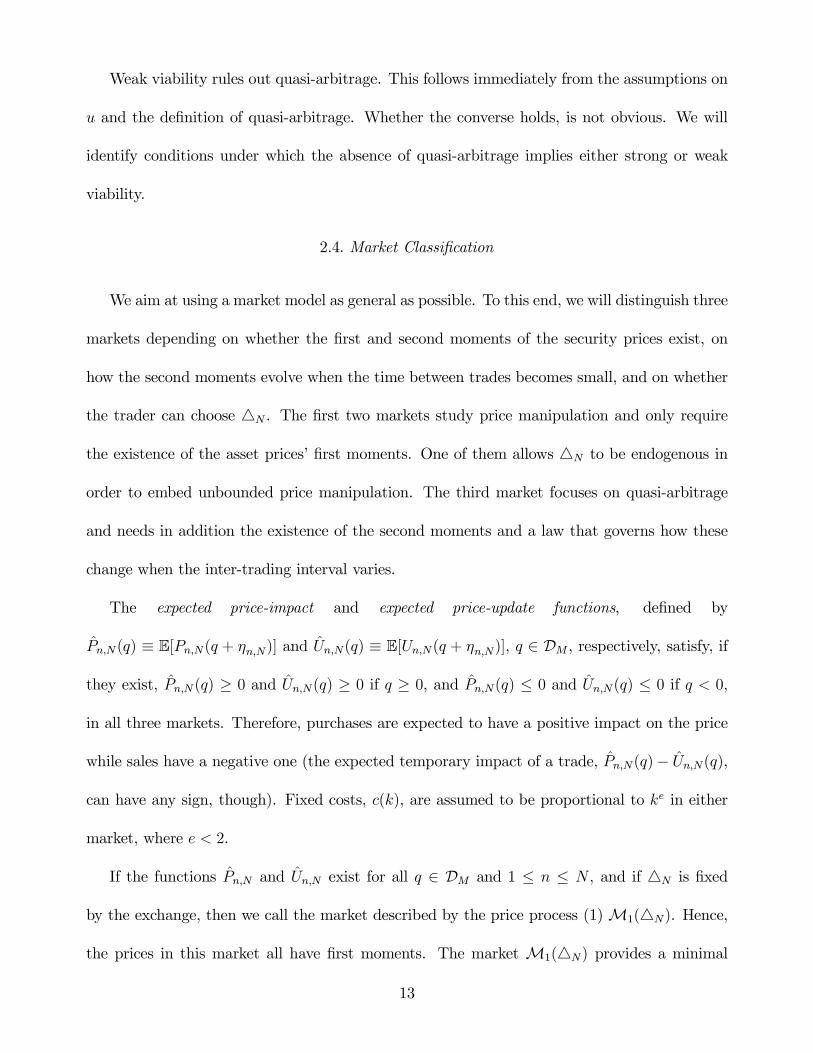
2.4. Market ClassiÞcation

We aim at using a market model as general as possible. To this end, we will distinguish three

markets depending on whether the Þrst and second moments of the security prices exist, on

how the second moments evolve when the time between trades becomes small, and on whether

the trader can choose 4N . The Þrst two markets study price manipulation and only require

the existence of the asset prices Þrst moments. One of them allows 4N to be endogenous in

order to embed unbounded price manipulation. The third market focuses on quasi-arbitrage

and needs in addition the existence of the second moments and a law that governs how these

change when the inter-trading interval varies.

The expected price-impact and expected price-update functions, deÞned by

Pn,N (q) ≡ E[Pn,N(q + ηn,N)] and Un,N(q) ≡ E[Un,N(q + ηn,N)], q ∈ DM , respectively, satisfy, if

they exist, Pn,N (q) ≥ 0 and Un,N(q) ≥ 0 if q ≥ 0, and Pn,N(q) ≤ 0 and Un,N(q) ≤ 0 if q < 0,

in all three markets. Therefore, purchases are expected to have a positive impact on the price

while sales have a negative one (the expected temporary impact of a trade, Pn,N(q)− Un,N(q),

can have any sign, though). Fixed costs, c(k), are assumed to be proportional to ke in either

market, where e < 2.

If the functions Pn,N and Un,N exist for all q ∈ DM and 1 ≤ n ≤ N , and if 4N is Þxed

by the exchange, then we call the market described by the price process (1)M1(4N). Hence,

the prices in this market all have Þrst moments. The market M1(4N) provides a minimal

13

environment to study price manipulation.

In the second market, M1, not only all Pn,N s and Un,N s exist for N ≥ 1, 1 ≤ n ≤ N ,

but also the trader can choose 4N (at time zero). Furthermore, we require that Un,N(q) ≥

− Un,N(−q) for all non-negative q ∈ DM . This inequality says that purchases have an expected

price update no smaller than sales. It can be interpreted in various ways. One argument is

that sales often occur because of liquidity shocks and thus have less informational content. Or,

purchases have to have at least as big a price impact as sales, on average, because otherwise

the price would be expected to drop to zero in case buys and sells are equally likely. In market

M1 we will examine unbounded price manipulation.

Finally, the marketM1 shall be labeledM2 if also the variances VP (q, n,N) ≡ V ar[Pn,N (q+

ηn,N)], VU(q, n,N) ≡ V ar[Un,N(q + ηn,N)], and σ2ε(N) ≡ V ar[ε1,N ] (recall that V ar[εn,N ] is

constant for 1 ≤ n ≤ N) exist for all q ∈ DM , N ≥ 1, and 1 ≤ n ≤ N , and if the variances,

as a function of N , do not grow faster than linearly as N → ∞, for each q ∈ DM and n (see

Appendix A for details). We will determine under which conditions quasi-arbitrage is absent

in marketM2.

Standard models typically assume that σ2ε asymptotically evolves as 1/N (e.g., see Merton

(1990)), which say that the total variance of the asset price during a Þxed time horizon is

evenly divided between the N per-period variances of that asset. In contrast, this work permits

more general behavior of the variances. For instance, M2 admits σ2ε to be constant, which

allows the total variance, σ2ε(N)N , to be linearly increasing in the number of trades. Such an

assumption is appropriate if market volatility rises due to a higher trading intensity. At most,

the per-period variances inM2 can grow linearly in N , or put differently, the total variances

during the time interval (0, 1] can grow no more than quadratically in N .

14

The conditions introduced above are not restrictive and examples of the three markets can

be quite easily constructed. In any case,M2 is contained inM1, which, in turn, is a subset of

M1(4N), for all 4N .

3. SINGLE-ASSET TIME-INDEPENDENT PRICE IMPACT

The price-impact and price-update functions are time-independent if Pn,N = P and Un,N =

U for all N ≥ 1 and 1 ≤ n ≤ N .

3.1. Necessary Conditions for the Absence of Quasi-Arbitrage

We Þrst show that the absence of price manipulation in marketM1(4N) requires the price-

update function to be linear. To this end, allow for any trade size for the trader and assume

the crowds trades are normally distributed. The arguments below offer an outline of the proof

using four steps. The formal proof is in Appendix B.

CLAIM 1: The expected price-update function must be symmetric, i.e., U(q) = − U(−q). To

show this, note that either U(q) > − U(−q) or U(q) < − U(−q) for a q > 0 would invite price

manipulation. In the former case (where purchasing q units has a stronger impact on the price

update than selling q units), a trader could buy q shares in each of the Þrst m periods and

then sell q shares in each of the subsequent m periods (2m ≤ N). The expected proÞt of this

round-trip strategy satisÞes

(5) E[π(q0,N)] =m2

2q[ U(q) + U(−q)]− m

2q[ U(−q)− U(q) + 2( P (q)− P (−q))]− c(2m).

(Two additional technical assumptions (see conditions (C1) and (C3) in Appendix B) ensure

15

that this and all round-trip trades below induce only non-negative expected prices.) Hence, if

4N is sufficiently small, then E[π(q0,N)] > 0 and there is price manipulation.

In the second case, the reverse strategy (Þrst selling q shares in each of the Þrst m periods

and then buying back q shares in each of periods m+ 1 to 2m) would yield E[π(q0,N)] > 0 for

sufficiently small 4N .

It is straightforward to check that U(0) = 0, which concludes the proof of Claim 1.

CLAIM 2: U is continuous everywhere except possibly at the origin, i.e., lim j→∞ U(qj) = U(q),

q 6= 0, when limj→∞ qj = q. To sketch the idea of this part of the proof, consider the following

example. Suppose that the price-update function has an upward jump at q > 0, that is,

limqj↓q U(qj) > U(q). The strategy of buying qj > q shares in each of the Þrst m periods and

selling q shares in each of the following m periods, and selling the remaining shares at time

2m+1, where qj is chosen arbitrarily close to q, yields E[π(q0,N)] > 0 for sufficiently small 4N .

Due to the jump, the updating reacts less to sales than to buys, causing the average selling

price to exceed the average purchasing price. Appendix B demonstrates that for any possible

type of jump price manipulations can be found.

CLAIM 3: U is linear, since either U(q) > U(1)q or U(q) < U(1)q would induce price

manipulation, for an arbitrary q. To see this, consider the Þrst case and note that q > 0 can

be assumed to be a rational number. Now, buying q shares in each of the Þrst m periods

and then selling one share in each of the following mq periods (mq can be chosen to be an

integer) constitutes a price manipulation for sufficiently small 4N , because the selling moves

the price down by less than the degree to which the buying shifts the price upwards. The second

inequality can be rejected analogously.

CLAIM 4: U is linear. For this purpose, deÞne RU(q) ≡ U(q)− U(q). Then, Claim 3 implies

16

E[RU(q + η1,N )] = 0 for all q, which in turn has RU = 0, as a consequence, thanks to the

normality of η1,N . Actually, the equality U(q) = U(q) holds only L(R)-almost everywhere,

where L(R) is the Lebesgue measure on R.

Exactly the same strategy can be applied to prove that also the absence of unbounded

price manipulation inM1 and the absence of quasi-arbitrage in M2 each imply the linearity

of the price-update function. For example, let us verify that the Þrst price manipulation used

to prove Claim 1 can be extended to a quasi-arbitrage in marketM2 if U(q) > − U(−q). The

expected proÞt, E[π(q0,N)], is of order m2 by (5), while its standard deviation is only of order

ma, a < 2, by inequality (10) in Appendix B. Thus, when the trader chooses 4N → 0, q0,N

becomes a quasi-arbitrage. Similarly, all other price manipulations above can be augmented to

quasi-arbitrages if U deviates from linearity. For the details of these arguments and the proof

of the following proposition see Appendix B.

PROPOSITION 1: Suppose that any trade size is allowed for the trader and that either

(i) P[η1,N = 0] = 1 (zero net trades of the crowd) or

(ii) the crowds trades are normally distributed.

Then, the absence of price manipulation in M1(4N) requires U to be linear with non-negative

slope, L(R) − a.e., for all sufficiently small 4N . The linearity of U with non-negative slope

is also implied by each the absence of unbounded price manipulation in M1 and the absence of

quasi-arbitrage in M2.

Let us now generalize the previous results in two ways. First, the domains D, DM , Dη, and

Dε need no longer be R. Instead, each of them can be an arbitrary symmetric set (a set D

is symmetric if 0 ∈ D and q ∈ D implies −q ∈ D). Second, the distribution of the crowds

trading volume can be non-normal. To establish a generalization of Proposition 1 the following

17

deÞnition is useful.

DEFINITION 5: A function f : D → R is quasi-linear if it has the representation f(y) =

λy + Rf(y) on D, λ ≥ 0, L(D)-a.e., where the D-Borel-measurable function Rf : D → R

satisÞes

(6) En,N [Rf (qn,N + ηn,N)] = 0

for all G(N)n4N-measurable random variables qn,N : Ω→ DM , 1 ≤ n ≤ N, N ≥ 1. We call Rf the

residual function of f .

We will interpret this deÞnition after Theorem 1. However, note that any linear function

with non-negative slope is also quasi-linear and that equation (6) does not imply Rf = 0 (see

Appendix C).

Having DeÞnition 5, the proof of Proposition 1 can be easily modiÞed to give the theorem

below.

THEOREM 1: The absence of price manipulation inM1(4N) (NoPM) requires U to be quasi-

linear, if 4N is sufficiently small. The quasi-linearity of U is also a consequence of each, the

absence of unbounded price manipulation in M1 (NoUM), and the absence of quasi-arbitrage

in M2 (NoQA).

Theorem 1 says that each of (NoPM)-(NoQA) implies a price-update function that can

be written as the sum of a linear function and its residual function RU , which in conditional

expected terms drops out. The latter holds regardless of what order the trader submits, be-

cause the traders strategy set is identical to the set consisting of all G(N)n4N-measurable random

variables. Thus, traders always expect linear price updating.

18

One important formal feature of the price process (1) is that the price-impact function P can

be chosen to include Þxed per-share transaction costs. Therefore, Proposition 1 and Theorem

1 are also valid when commissions have to be paid per share.

Some empirical papers report evidence of asymmetric price impacts. For instance, Chan

and Lakonishok (1995), Gemmill (1996), and Holthausen et al. (1987, 1990) Þnd that block

purchases have a larger price impact than block sales, whereas Keim and Madhavan (1996)

and Scholes (1972) provide evidence that there are also markets with a stronger price impact

of sales. A literal interpretation of Proposition 1 and Theorem 1 suggests quasi-arbitrage.

Alternatively, this result suggests that a better speciÞcation should allow for time dependence

of the price-impact function.

Proposition 1 and Theorem 1 above establish the linearity of the price-update function.

Necessary conditions for the price-impact function are in Proposition 2. (Recall that the price-

impact function is the sum of the permanent component - the price-update function - and the

temporary component.)

PROPOSITION 2: If either (NoPM) or (NoUM) holds, and if Þxed costs c(k) are proportional

to ka, a < 1, then the following two conditions must hold for all sufficiently small 4N :

(i) P (q)− P (−q) R U(q) for q R 0, q ∈ DM , and

(ii) P 6= 0 when U 6= 0.

If we interpret the left-hand side of condition (i) in Proposition 2 as the expected spread of

the price-impact function, then condition (i) says that the expected spread at any trade size has

to exceed the expected price update resulting from that trade. Were this not true, the trading

strategy cited in the proof of Claim 1 (buying q shares in each of the Þrst m periods and then

selling q shares in each of the next m periods) would allow unbounded price manipulation (see

19

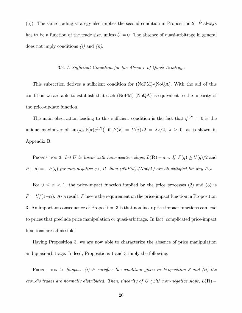
(5)). The same trading strategy also implies the second condition in Proposition 2. P always

has to be a function of the trade size, unless U = 0. The absence of quasi-arbitrage in general

does not imply conditions (i) and (ii).

3.2. A Sufficient Condition for the Absence of Quasi-Arbitrage

This subsection derives a sufficient condition for (NoPM)-(NoQA). With the aid of this

condition we are able to establish that each (NoPM)-(NoQA) is equivalent to the linearity of

the price-update function.

The main observation leading to this sufficient condition is the fact that q0,N = 0 is the

unique maximizer of supq0,N E[π(q0,N)] if P (x) = U(x)/2 = λx/2, λ ≥ 0, as is shown in

Appendix B.

PROPOSITION 3: Let U be linear with non-negative slope, L(R)− a.e. If P (q) ≥ U(q)/2 and

P (−q) = −P (q) for non-negative q ∈ D, then (NoPM)-(NoQA) are all satisÞed for any 4N .

For 0 ≤ α < 1, the price-impact function implied by the price processes (2) and (3) is

P = U/(1−α). As a result, P meets the requirement on the price-impact function in Proposition

3. An important consequence of Proposition 3 is that nonlinear price-impact functions can lead

to prices that preclude price manipulation or quasi-arbitrage. In fact, complicated price-impact

functions are admissible.

Having Proposition 3, we are now able to characterize the absence of price manipulation

and quasi-arbitrage. Indeed, Propositions 1 and 3 imply the following.

PROPOSITION 4: Suppose (i) P satisÞes the condition given in Proposition 3 and (ii) the

crowds trades are normally distributed. Then, linearity of U (with non-negative slope, L(R)−

20

a.e.) is equivalent to the absence of price manipulation in M1(4N), for all sufficiently small

4N . The linearity of U (with non-negative slope, L(R)−a.e.) is also equivalent to each (NoUM)

and (NoQA).

Proposition 4 connects (NoPM)-(NoQA) through one common characterizing property,

namely, the linearity of the price-update function.

3.3. Strong Viability

Proposition 4 and the observation made before Proposition 3 enable us to determine when

marketsM1 andM2 are strongly or weakly viable.

COROLLARY 1: Assume that the conditions (i)-(ii) in Proposition 4 are met. Then, the

absence of quasi-arbitrage in market M2 is characterized by the strong viability of M2. If the

trader is risk-neutral, the strong viability of marketM1 is equivalent to the absence of unbounded

price manipulation in M1.

Proposition 4 and Corollary 1 can be directly applied to two problems which are often

studied in the Þnance microstructure literature. The Þrst involves insider trading, where a

monopolistic insider solves supqnNn=1E[PN

n=1(v−pn)qn] for a given N , after having received the

value of the asset, v, in period 0 (e.g., see Dutta and Madhavan (1995)). The second problem

is discretionary liquidity trading, as studied in Bertsimas and Lo (1998) and Huberman and

Stanzl (2002). There, an uninformed trader faces the problem infqnNn=1 E[PN

n=1 pnqn] subject toPNn=1 qn = q 6= 0, given the number of trades, N . In other words, this trader wants to minimize

the expected costs of trading a certain amount of shares, q, over a certain time horizon. These

studies employ a simpler version of the price process (3) with linear price-update functions.

Proposition 4 and Corollary 1 justify their linearity assumptions.

21

4. TIME-DEPENDENT PRICE IMPACT

Until now, the price-impact and price-update functions have been time-independent, i.e.,

price reacts to traded quantity in the same manner in each period. Liquidity, which is repre-

sented by the Þrst derivative of the price-impact and price-update functions (when they exist),

is therefore constant through time. In what follows we relax this assumption and allow liquidity

to vary across time.

4.1. Absence of Price Manipulation

One way to examine time-dependent liquidity is to consider linear price-impact and price-

update functions that change over time. More speciÞcally,

(7) pn,N = pn−1,N + λn−1,N(qn−1,N + ηn−1,N) + εn,N ,

pn,N = pn,N + µn,N(qn,N + ηn,N),

for sequences λn,NNn=1 and µn,NNn=1, where λ1,N = µ1,N ≥ 0. The price-impact and price-

update functions are allowed to have any sign, that is, the slopes λn,NNn=2 and µn,NNn=2 can

either be positive or negative.

We proceed by establishing an equivalent condition for the absence of price manipulation.

The main difference with the previous section is that unbounded price manipulation can usually

be implemented with Þnitely many trades. In contrast to the last section, we can employ the

global shape of the price-impact and price-update functions to seek for price manipulation.

To get an idea what kind of restrictions the absence of price manipulation imposes on the

pair (λn,NNn=1, µn,NNn=1), let us consider the simple case N = 3 where only three trades are

22

feasible. Computing E[π(q0,3)] for any round-trip trade q0,3 leads to

−E"

3Xn=1

[p0,3 +n−1Xj=1

λj,3(qj,3 + ηj,3) + µn,3(qn,3 + ηn,3) +nXj=1

εj,3]qn,3

#− c(T (q0,3))

= −E £µ2,3q22,3 + λ2,3q2,3q3,3 + µ3,3q23,3¤− c(T (q0,3))+ E

"2Xn=1

λn,3ηn,3

nXj=1

qj,3 −3Xn=1

µn,3qn,3ηn,3 +3Xn=2

εn,3

n−1Xj=1

qj,3

#,

which is −E £[q2,3 q3,3]Λ3[q2,3 q3,3]T ¤ /2− c(T (q0,3)), where

Λ3 ≡

2µ2,3 λ2,3

λ2,3 2µ3,3

.

The trades q2,3 and q3,3 in the above expression can take any value as long as the trades q1,3,

q2,3, and q3,3 do not cause negative expected prices. Hence, for all sufficiently large initial prices

p0,3, the absence of price manipulation is equivalent to Λ3 being positive semideÞnite.

The removal of q1,3 is arbitrary. If we remove q2,3 or q3,3, we would Þnd that

2µ2,3 2µ2,3 − λ2,3

2µ2,3 − λ2,3 2(µ2,3 − λ2,3 + µ3,3)

and

2µ3,3 2µ3,3 − λ2,3

2µ3,3 − λ2,3 2(µ2,3 − λ2,3 + µ3,3)

,

respectively, have to be positive semideÞnite to exclude price manipulation. Since all matrix

representations employ the same parameters and each matrix is positive semideÞnite if and

only if the others are, either matrix can be used for the analysis. We work here only with Λ3

henceforth.

For Λ3 to be positive semideÞnite, µ2,3 and µ3,3 must be non-negative and µ2,3µ3,3 ≥ λ22,3/4.

23

These conditions, together with µ1,3 ≥ 0, say that the absence of price manipulation rules out

negative price-impact sequences in all periods and that µ2,3 and µ3,3 have to be sufficiently large

relative to λ22,3.

The same method as above applied to the general case gives the following.

THEOREM 2: Fix an arbitrary 4N . For all sufficiently large initial prices p0,N , no price

manipulation in M1(4N) is characterized by the positive semideÞniteness of the matrix

(8) ΛN ≡

2µ2,N λ2,N λ2,N . . . λ2,N

λ2,N 2µ3,N λ3,N . . . λ3,N

λ2,N λ3,N 2µ4,N . . . λ4,N

......

.... . .

...

λ2,N λ3,N λ4,N . . . 2µN,N

.

Theorem 2 gives a speciÞc computational criterion for the absence of price manipulation.

Testing whether ΛN is positive semideÞnite can be easily done, unless N is too big. In any case,

we suggest to Þrst check whether ΛN is positive deÞnite. If Λj,N denotes the jth-order leading

principal submatrix of ΛN (delete the last N − 1− j rows and the last N − 1 − j columns of

ΛN), then detΛj,N > 0 for all 1 ≤ j ≤ N−1 if and only if ΛN is positive deÞnite. Each detΛj,N

can be obtained recursively from

(9) detΛj,N = 2(µj,N + µj−1,N − λj−1,N) detΛj−1,N − (2µj−1,N − λj−1,N)2 detΛj−2,N

for 3 ≤ j ≤ N−1, where ΛN−1,N = ΛN , with initial conditions detΛ1,N = 2µ2,N and detΛ2,N =

4µ2,Nµ3,N − λ22,N . Hence, the complexity of testing for positive deÞniteness is only of linear

24

order.

Another important implication of Theorem 2 is that for any given price-update sequence

there exists a price-impact sequence that preserves the absence of price manipulation. This is

a consequence of the price-update and price-impact slopes being different: the µn,N s only have

to be chosen high enough, according to (9).

While all µn,N s must be non-negative, the signs of the λn,N s are ambiguous. Negative

λn,N s are in discord with the interpretations that purchases either signal good news about

the assets value, or assert positive price pressure due to a declining inventory of the liquidity

providers. But in this context negativity makes sense. The main mechanism that makes price

manipulation successful is the positive relation between price update and trading volume. If

the λn,N s are negative, this mechanism would not work any more. For example, a purchase

that drives up the price today but moves down future prices would erode the traders ability

to make money from trading.

The condition put forward in Theorem 2 is easiest interpreted when temporary price impacts

are absent (λn,N = µn,N for 1 ≤ n ≤ N). In this case, a positive semideÞnite ΛN implies that

liquidity cannot increase over time by too high a rate. Otherwise, the trader could lock in

expected proÞts from price manipulation: he begins pushing up the price in the early illiquid

periods by consecutive purchases until the market becomes more liquid. He then sells the shares

he is holding and makes proÞts since, due to the more liquid market, he can do the selling at an

average price higher than the average purchase price. On the other hand, if liquidity decreases

over time, price manipulation is infeasible. For instance, selling shares in the Þrst periods and

buying them back in later, less liquid periods would be unproÞtable, because the purchase

prices would exceed the selling prices on average.

25

Unfortunately, there is no handy characterizing condition for the absence of unbounded price

manipulation or quasi-arbitrage. As a consequence, one has to verify whether quasi-arbitrage is

possible for each individual case. However, this task is in general not too difficult, because the

price-update and price-impact functions are linear. Here is an example. Consider p0,N = 10,

λn,33n=1 = µn,33n=1 with λ1,3 = λ2,3 = 1 and λ3,3 = 0. Buying q units of the asset in each of

periods 1 and 2, and then selling the holdings in the third period results in expected proÞts of

E[π(q0,3)] = −(10+ q)q− (10+2q)q+2q(10+2q) = q2, while Std[π(q0,3)] = qqσ2η(3) + 5σ

2ε(3).

Hence, E[π(q0,3)] → ∞ and SR[π(q0,3)] → ∞ as q → ∞. Such prices would not be weakly

viable.

REMARK: Breen et al. (2002), Chen et al. (2002), and Hasbrouck (1991) estimate the relation

between prices and trading volume by employing price-impact functions which differ from ours.

Theorems 1 and 2 are thus inapplicable to their models. Yet, a test for price manipulation

can be easily conducted. Given their parameter estimates and reasonable assumptions on the

levels of 4N and Þxed transaction costs, price manipulation is feasible in each model. In such

circumstances, empirical papers should either impose parameter conditions that exclude quasi-

arbitrage or drop the assumption that the sequence of past trades does not affect the shape of

the current price-impact function.

REMARK: Nonlinear, time-dependent price-update functions may assume chaotic shapes

without giving rise to price manipulation. Only when additional assumptions are made on the

shapes of the price-update functions the analysis becomes meaningful. We focus here on linear

price-impact and price-update functions, but one could impose other restrictions.

In the next subsection we will examine the insider trading problem based on the Kyle (1985)

model in more detail.

26

4.2. Discussion of the Kyle Model

Black (1995) conjectures that the Kyle (1985) model allows arbitrage opportunities for

uninformed agents if they pretend to be informed. We will prove that this conjecture is wrong

and that the equilibrium price-update functions in Kyle must be linear asymptotically under

certain conditions.

Kyles model describes a game between competitive market-makers, who set the price in each

period, and an individual risk-neutral insider trader, who has information on the liquidation

value v > 0 of the single asset that is traded. The framework is as follows. All trades take

place in the time interval [0, 1] and the insider can choose any trade size. In each period, the

market-makers observe only the aggregate trading volume, which is the sum of the insiders

trading quantity and crowds trades. They cannot observe the insiders amounts. Knowing the

history of trades and the fact that there is one risk-neutral informed trader who maximizes his

proÞts, they set the price equal to the conditional expected value, that is, pn,N = E[v | F (N)n4N]

for 1 ≤ n ≤ N . The insider, on the other hand, taking into account how the market-makers

compute the price, submits in each round the quantity qn,N that maximizes his proÞts.

As Kyle shows for the case of normally and independently distributed trading volume of

the crowd, this game has a unique linear equilibrium where the price evolves according to

pn,N = pn−1,N + λn,N(qn,N + ηn,N), the liquidity parameters λn,N being endogenously (but

deterministically) determined. But this price process is just a special case of (7) if the price

impact has no temporary component and εn,N = 0. Thus, Theorem 2 can be applied to Kyle.

For any 4N , Kyles slopes are almost constant and hence price manipulation is infeasible.

Consequently, Kyles equilibrium is strongly viable.

One can extend the Kyle model with one insider by allowing prices that incorporate more

27

general nonlinear price-update functions, like pn,N = pn−1,N + Un,N (qn,N + ηn,N ) + εn,N (the

price process given in (3)). Since the absence of unbounded price manipulation is necessary in

equilibrium, it can be used to Þnd the shape of equilibrium price-update functions.

PROPOSITION 5: Suppose the price-update functions Un,NNn=1 are symmetric, i.e., Un,N(x) =

−Un,N(−x) ≥ 0, x ≥ 0, and monotone in the sense that Un,N (x) ≤ Un−1,N(x) for x ≥ 0. Then,

given the price dynamics in (3), the absence of unbounded price manipulation in M1 implies

that the expected price-update functions converge pointwise to a linear function on any interval

(τ , 1− τ ), 0 < τ < 1/2, as N →∞. More formally, for any ε > 0 and x ∈ R there exists an

index N0 such that for N ≥ N0¯Un,N(x)− λx

¯< ε, with τ ≤ n/N ≤ 1− τ , λ ≥ 0.

The monotonicity assumption implies that the insiders optimal policy causes the market

maker to react less sensitively to trade size over time. This assumption is motivated by the

properties of the linear equilibrium in Kyle.

Thus, as the number of auctions, N , becomes very large, only equilibria with approximately

linear expected price-update functions are sustainable.

5. MULTIPLE ASSETS

So far we have discussed price manipulation and quasi-arbitrage only for one Þnancial asset,

but in typical applications investors trade many assets at the same time. In this section we

extend our approach to the multivariate setting where a portfolio ofK > 1 assets can be traded.

The price-impact and price-update functions are assumed to be time-independent.

The multivariate case contains several interesting features not captured by the single-asset

analysis. Presumably, the most important one is the ability to incorporate cross-price impact

28

functions: the traded quantity of asset i affects not only the price of asset i but also the prices

of other assets.

To extend formally the single-asset model to a multidimensional one, just replace all (single-

valued) variables by K-dimensional vectors. In particular, the price-impact and price-update

functions take each the traded quantities of the K assets as arguments, and map to a K vector,

where component j gives the price-impact and price-update functions for asset j, respectively.

Further, the non-negative slope λ in the deÞnition of quasi-linearity (see DeÞnition 5 above)

now is a positive semideÞnite matrix.

As the following example illustrates, cross-price-impact functions may lead to price manip-

ulation. Suppose that there are two assets A and B, that only one share can be traded, and

that price-impact functions are permanent. Table I shows a price-impact function for these two

assets which exhibits asymmetric cross-price impacts. If one share of A is bought and none of

B, then the price of A increases by one dollar and that of B by 50 cents. On the other hand,

if one purchases one share of B and none of A, only the price of B rises (by one dollar). Now,

buying one share of asset B in each of the Þrst three periods, buying one share of A in each of

the next eight periods, selling one share of B in each of the following three periods, and then

selling one share of A in the subsequent eight periods, yields a proÞt of one dollar on average.

INSERT TABLE I ABOUT HERE

All results stated in Theorem 1 and Propositions 1 and 4 regarding the absence of price

manipulation inM1(4N) are literally true for the multi-asset case. Only Proposition 4 has to

be adjusted slightly. Instead of condition (i) we impose U = P (no temporary price impacts)

as a sufficient condition.

Thus, the absence of price manipulation is equivalent to the price-impact function being

29

linear, represented by a positive semideÞnite matrix. In particular, all cross-price impact func-

tions are linear and pairwise symmetric, that is, the price impact of asset i on asset j is the

same as the price impact of asset j on asset i.

The concept of unbounded price manipulation or quasi-arbitrage is less applicable here.

Trading inÞnite amounts introduces a technical difficulty of the following sort. Suppose there

exists a quasi-arbitrage for asset A in the single-asset world. Introduce another asset B whose

price goes down whenever asset A is bought. Since a quasi-arbitrage typically requires to buy a

certain amount of shares of asset A inÞnitely many times, the price of B will eventually become

negative, even if the negative price impact on B is tiny. To avoid such cases we would need

to make additional assumptions about prices. We refrain from doing that in order not to lose

generality. Anyway, price manipulation can become fairly large if the trade of an asset has a

considerably larger impact on its own price than on the prices of other assets.

Black (1995) informally argues that the sum of the price update of individual trades must

equal the price update of trading the basket containing these individual trades. In other

words, the price update must be an additive function in the trading volume. Our results

demonstrate that eliminating price manipulation requires more structure on the shape of the

price-update function than Black claims.

6. PRICE MANIPULATION AND THE GAIN-LOSS RATIO

Bernardo and Ledoit (2000) propose to use the gain-loss ratio of an investment as a

measure of its attractiveness. It is deÞned as the expectation of the investments positive excess

payoffs divided by the expectation of its negative excess payoffs. More formally, if z denotes

the payoff of a zero-cost portfolio, then the gain-loss ratio equals GLR[z] ≡ E[z+]/E[z−], where

30

z+ = max(z, 0) and z− = max(−z, 0). One advantage of using the gain-loss ratio to detect

attractive investment opportunities, rather than the Sharpe ratio, is that it recognizes a pure

arbitrage with fat upper tails and ßat lower tails as desirable, while the Sharpe ratio may not.

In the framework of Bernardo and Ledoit (2000) the absence of pure arbitrage is equivalent

to the gain-loss ratio being Þnite. Thus, by imposing an upper bound on the gain-loss ratio

arbitrage opportunities are ruled out. Even though our model generally does not exhibit this

equivalence, one might want to exclude round-trip trades, q0,Nm ∞m=1, with limm→∞E[π(q0,Nm )] =

limm→∞GLR[π(q0,Nm )] =∞. The existence of such great deals may threaten market viability.

To analyze great deals, we focus here only on time-independent price-impact and price-

update functions. The market environment is described byM∗1 which isM2 with the difference

that the growth conditions (as 4N becomes small) are imposed on the negative part of the

random variables involved rather than on their variances (see Appendix A).

Everything derived in Section 3 for the absence of quasi-arbitrage in marketM2 also applies

to the absence of great deals in marketM∗1. More precisely, all statements made in Theorem

1 and Propositions 1, 3, and 4 regarding the absence of quasi-arbitrage inM2 are also true for

the absence of great deals in M∗1. Hence, linearity of the price-update function is necessary

to rule out great deals. It is also sufficient for the absence of great deals if the conditions in

Proposition 4 are met.

In order to examine market viability, suppose that the traders utility is given by

u(GLR[π(q0,N)]), where u is strictly increasing and GLR[π(0)] ≡ 1. The following result,

which resembles Corollary 1, can be easily deduced when conditions (i)-(ii) in Proposition 4 are

satisÞed. The absence of great deals inM∗1 is equivalent to the strong viability ofM∗

1.

31

7. CONCLUDING REMARKS

This paper studies price manipulation and quasi-arbitrage for markets where trade size

moves the price and prices are uncertain when trades are placed. A price manipulation and a

quasi-arbitrage are both round-trip trading strategies, where the Þrst creates a positive expected

payoff, while the second produces an inÞnite expected payoff, as well as an inÞnite Sharpe ratio.

Markets with time-independent price-impact functions are strongly viable if and only if there

is no quasi-arbitrage, when agents utility is measured by the Sharpe ratio of an investment

opportunity.

We examine the conditions imposed by the absence of quasi-arbitrage on the functional

shape of the temporary and permanent price effect of a trade. If the price-impact and price-

update functions are time-independent and certain multiples of each other, then the absence

of quasi-arbitrage is equivalent to the linearity of both functions. On the other hand, if the

price-impact and price-update functions are independent, then only the price-update function

must be linear in trading volume, while the temporary price impact can have various forms

without offering quasi-arbitrage opportunities.

The theoretical microstructure literature usually assumes that the change in prices is time-

independent and reacts linearly to trading volume. This paper demonstrates that the assump-

tion of time independence of price changes already implies the linearity of the price-update

function.

Linearity as a necessary condition for the absence of quasi-arbitrage calls for a careful

examination of empirical estimations of price-update functions. To the extent that they detect

deviations from linearity, one may wonder why some price manipulation possibilities had gone

unexploited or one can suspect some misspeciÞcation (perhaps a time-dependent environment).

32

Postulating a Þnite gain-loss ratio instead of the absence of quasi-arbitrage does not change

any of our conclusions. Also in this case the price-update function has to be linear, since

otherwise the gain-loss ratio would become inÞnite.

The results of this paper call for one main extension, namely to permit the trading of

market and limit orders at the same time. How do limit orders affect the market price? And

what does a no-arbitrage condition look like if traders can submit market and limit orders

simultaneously? Most important, we would like to examine how market and limit orders can

coexist in an equilibrium exchange.

Columbia Business School, 3022 Broadway, New York, NY 10027,

and

Ziff Brothers Investments, L.L.C., 153 East 53rd Street, 43rd Floor, New York, NY 10022.

33

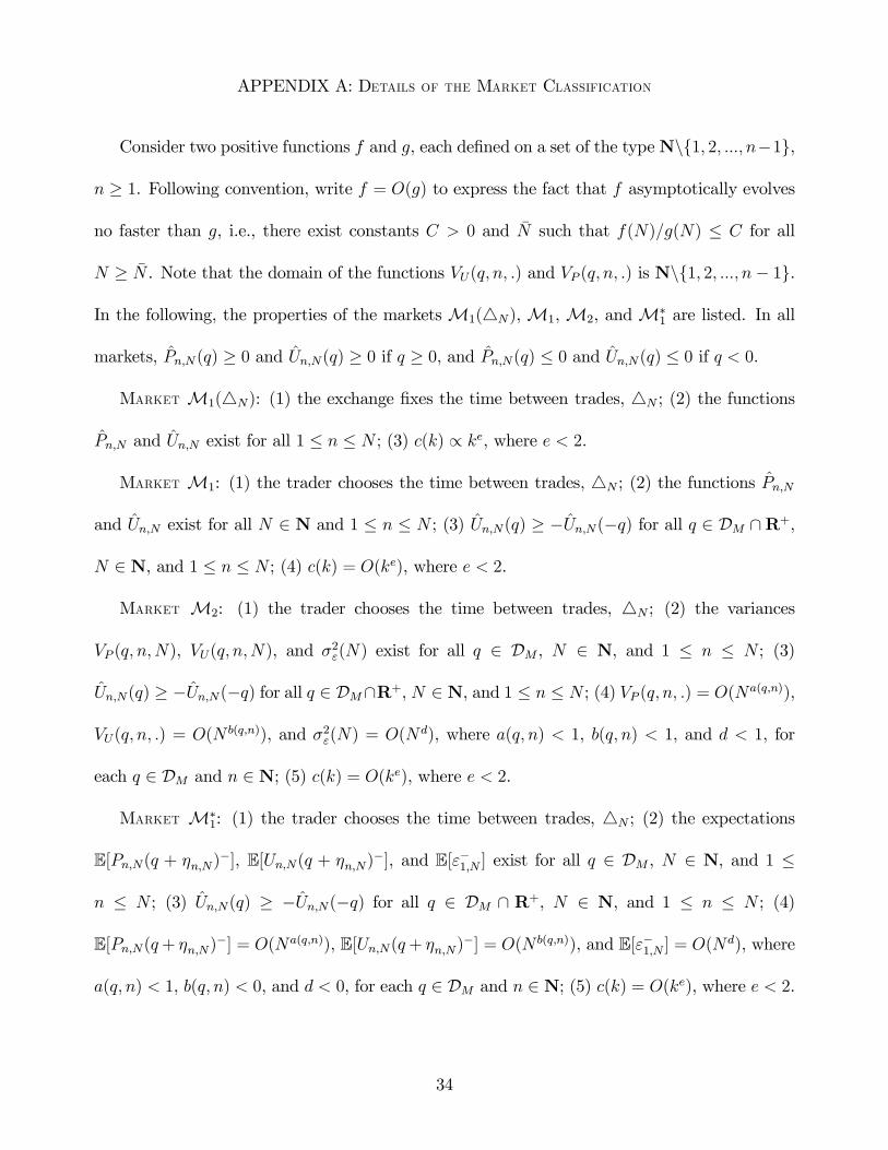
APPENDIX A: DETAILS OF THE MARKET CLASSIFICATION

Consider two positive functions f and g, each deÞned on a set of the typeN\1, 2, ..., n−1,

n ≥ 1. Following convention, write f = O(g) to express the fact that f asymptotically evolves

no faster than g, i.e., there exist constants C > 0 and N such that f(N)/g(N) ≤ C for all

N ≥ N . Note that the domain of the functions VU(q, n, .) and VP (q, n, .) is N\1, 2, ..., n− 1.

In the following, the properties of the marketsM1(4N),M1,M2, andM∗1 are listed. In all

markets, Pn,N (q) ≥ 0 and Un,N(q) ≥ 0 if q ≥ 0, and Pn,N(q) ≤ 0 and Un,N(q) ≤ 0 if q < 0.

MARKET M1(4N): (1) the exchange Þxes the time between trades, 4N ; (2) the functions

Pn,N and Un,N exist for all 1 ≤ n ≤ N ; (3) c(k) ∝ ke, where e < 2.

MARKET M1: (1) the trader chooses the time between trades, 4N ; (2) the functions Pn,N

and Un,N exist for all N ∈ N and 1 ≤ n ≤ N ; (3) Un,N(q) ≥ − Un,N(−q) for all q ∈ DM ∩R+,

N ∈ N, and 1 ≤ n ≤ N ; (4) c(k) = O(ke), where e < 2.

MARKET M2: (1) the trader chooses the time between trades, 4N ; (2) the variances

VP (q, n,N), VU(q, n,N), and σ2ε(N) exist for all q ∈ DM , N ∈ N, and 1 ≤ n ≤ N ; (3)

Un,N(q) ≥ − Un,N(−q) for all q ∈ DM∩R+, N ∈ N, and 1 ≤ n ≤ N ; (4) VP (q, n, .) = O(Na(q,n)),

VU(q, n, .) = O(N b(q,n)), and σ2ε(N) = O(Nd), where a(q, n) < 1, b(q, n) < 1, and d < 1, for

each q ∈ DM and n ∈ N; (5) c(k) = O(ke), where e < 2.

MARKET M∗1: (1) the trader chooses the time between trades, 4N ; (2) the expectations

E[Pn,N(q + ηn,N)−], E[Un,N(q + ηn,N)−], and E[ε−1,N ] exist for all q ∈ DM , N ∈ N, and 1 ≤

n ≤ N ; (3) Un,N(q) ≥ − Un,N(−q) for all q ∈ DM ∩ R+, N ∈ N, and 1 ≤ n ≤ N ; (4)

E[Pn,N(q+ ηn,N)−] = O(Na(q,n)), E[Un,N(q+ ηn,N)−] = O(N b(q,n)), and E[ε−1,N ] = O(Nd), where

a(q, n) < 1, b(q, n) < 0, and d < 0, for each q ∈ DM and n ∈ N; (5) c(k) = O(ke), where e < 2.

34

APPENDIX B: PROOFS OF THE RESULTS IN SECTIONS 3-5

Before proving Proposition 1 and Theorem 1, we derive two helpful results. To simplify the

analysis, we make three technical assumptions:

(C1) If a sale is expected to induce a negative transaction price, then the expected revenue

from this sale is set equal to zero;

(C2) If q ∈ DM is irrational, then there exists at least one sequence qj∞j=1 such that all

qj ∈ DM ∩Q and limj→∞ qj = q;

(C3) P[ε1,N > a] > 0 for all a > 0 and N ∈ N.

LEMMA 1: Each of the conditions (NoPM)-(NoQA) in Theorem 1 implies:

(i) U is symmetric on DM , i.e., U(q) = − U(−q) for q ∈ DM ; and

(ii) lim j→∞ U(qj) = U(q) if limj→∞ qj = q 6= 0.

PROOF: To verify (i) we start by proving that U (q) ≤ − U (−q) holds for all positive q ∈ DM .

Suppose that this is not true, that is, there exists a q > 0 with U (q) > − U (−q). Implement

now the following trading strategy q0,N : buy in each of the Þrst m periods the volume q, and

then sell the quantity q in each of the next m periods. This round-trip strategy implies non-

negative expected prices and an expected proÞt given by (5). Therefore, if 4N is sufficiently

small and 2m ≤ N , E[π(q0,N)] > 0 and price manipulation is feasible.

If the variances exist, we can calculate

(10) V ar[π(q0,N)] ≤ q2½m(m+ 1)(2m+ 1)

6VU(q) +mVP (q) +m(m+ 1)

pVU(q)VP (q)

+(m− 1)m(2m− 1)

6VU(−q) +mVP (−q) +m(m− 1)

pVU(−q)VP (−q) + m(2m

2 + 1)

3σ2ε(N)

¾

35

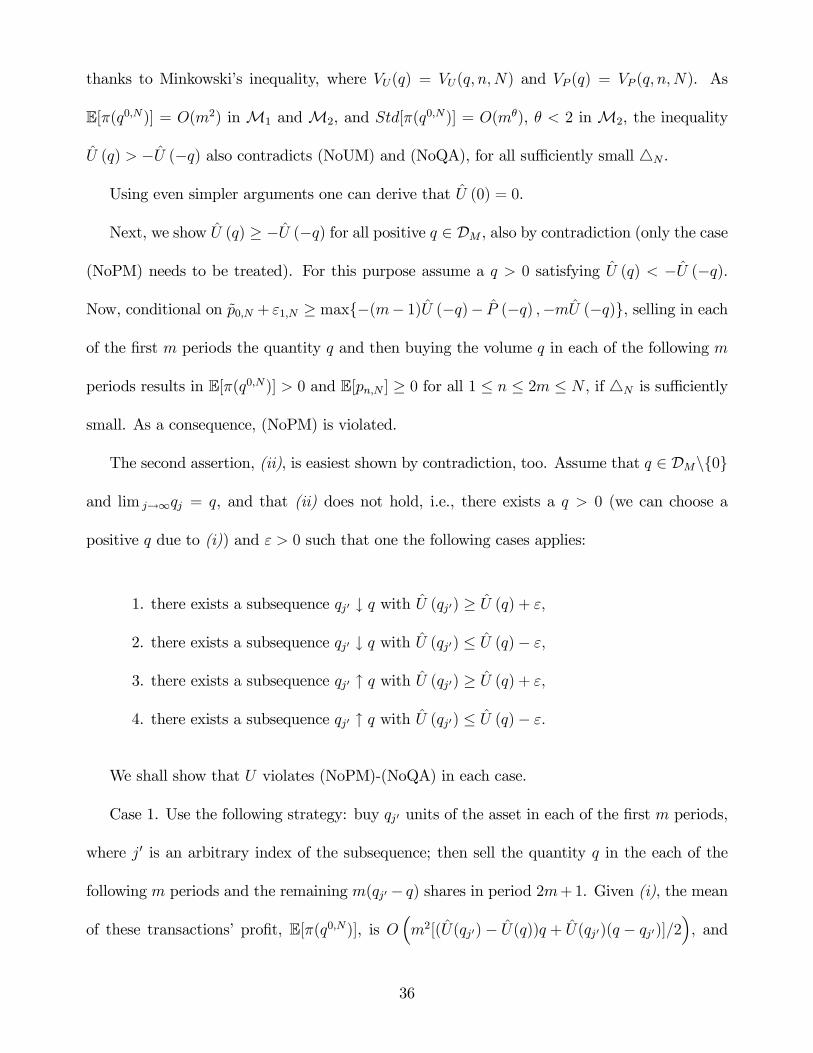
thanks to Minkowskis inequality, where VU(q) = VU(q, n,N) and VP (q) = VP (q, n,N). As

E[π(q0,N)] = O(m2) inM1 andM2, and Std[π(q0,N)] = O(mθ), θ < 2 inM2, the inequality

U (q) > − U (−q) also contradicts (NoUM) and (NoQA), for all sufficiently small 4N .

Using even simpler arguments one can derive that U (0) = 0.

Next, we show U (q) ≥ − U (−q) for all positive q ∈ DM , also by contradiction (only the case

(NoPM) needs to be treated). For this purpose assume a q > 0 satisfying U (q) < − U (−q).

Now, conditional on p0,N + ε1,N ≥ max−(m− 1) U (−q)− P (−q) ,−m U (−q), selling in each

of the Þrst m periods the quantity q and then buying the volume q in each of the following m

periods results in E[π(q0,N)] > 0 and E[pn,N ] ≥ 0 for all 1 ≤ n ≤ 2m ≤ N , if 4N is sufficiently

small. As a consequence, (NoPM) is violated.

The second assertion, (ii), is easiest shown by contradiction, too. Assume that q ∈ DM\0

and lim j→∞qj = q, and that (ii) does not hold, i.e., there exists a q > 0 (we can choose a

positive q due to (i)) and ε > 0 such that one the following cases applies:

1. there exists a subsequence qj0 ↓ q with U (qj0) ≥ U (q) + ε,

2. there exists a subsequence qj0 ↓ q with U (qj0) ≤ U (q)− ε,

3. there exists a subsequence qj0 ↑ q with U (qj0) ≥ U (q) + ε,

4. there exists a subsequence qj0 ↑ q with U (qj0) ≤ U (q)− ε.

We shall show that U violates (NoPM)-(NoQA) in each case.

Case 1. Use the following strategy: buy qj0 units of the asset in each of the Þrst m periods,

where j0 is an arbitrary index of the subsequence; then sell the quantity q in the each of the

following m periods and the remaining m(qj0 − q) shares in period 2m+1. Given (i), the mean

of these transactions proÞt, E[π(q0,N)], is O³m2[( U(qj0)− U(q))q + U(qj0)(q − qj0)]/2

´, and

36

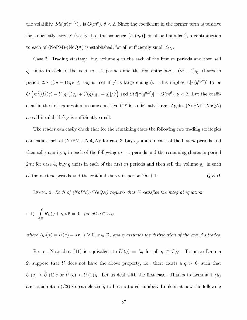
the volatility, Std[π(q0,N )], is O(mθ), θ < 2. Since the coefficient in the former term is positive

for sufficiently large j0 (verify that the sequence U (qj0) must be bounded!), a contradiction

to each of (NoPM)-(NoQA) is established, for all sufficiently small 4N .

Case 2. Trading strategy: buy volume q in the each of the Þrst m periods and then sell

qj0 units in each of the next m − 1 periods and the remaining mq − (m − 1)qj0 shares in

period 2m ((m− 1) qj0 ≤ mq is met if j0 is large enough). This implies E[π(q0,N)] to be

O³m2[( U(q)− U(qj0))qj0 + U(q)(qj0 − q)]/2

´and Std[π(q0,N)] = O(mθ), θ < 2. But the coeffi-

cient in the Þrst expression becomes positive if j0 is sufficiently large. Again, (NoPM)-(NoQA)

are all invalid, if 4N is sufficiently small.

The reader can easily check that for the remaining cases the following two trading strategies

contradict each of (NoPM)-(NoQA): for case 3, buy qj0 units in each of the Þrst m periods and

then sell quantity q in each of the following m− 1 periods and the remaining shares in period

2m; for case 4, buy q units in each of the Þrst m periods and then sell the volume qj0 in each

of the next m periods and the residual shares in period 2m+ 1. Q.E.D.

LEMMA 2: Each of (NoPM)-(NoQA) requires that U satisÞes the integral equation

(11)ZΩ

RU(q + η)dP = 0 for all q ∈ DM ,

where RU(x) ≡ U(x)− λx, λ ≥ 0, x ∈ D, and η assumes the distribution of the crowds trades.

PROOF: Note that (11) is equivalent to U (q) = λq for all q ∈ DM . To prove Lemma

2, suppose that U does not have the above property, i.e., there exists a q > 0, such that

U (q) > U (1) q or U (q) < U (1) q. Let us deal with the Þrst case. Thanks to Lemma 1 (ii)

and assumption (C2) we can choose q to be a rational number. Implement now the following

37

trading strategy: buy q units of the asset in each of the Þrst m periods such that mq is an

integer, then sell one unit in each of the following mq periods (m(1 + q) ≤ N). It follows that

E[π(q0,N)] = O(m2q[ U(q) − U(1)q]/2) and Std[π(q0,N)] = O(mθ), θ < 2, contradicting each of

(NoPM)-(NoQA), if 4N is sufficiently small.

The case U (q) < U (1) q can be tackled similarly: it is easy to verify that the strategy of

buying one unit in each of the Þrst mq periods and then selling q units in each of the next m

periods results in a violation of each (NoPM)-(NoQA). Q.E.D.

PROOF OF THEOREM 1: Immediate consequence of Lemmas 1 and 2. Q.E.D.

PROOF OF PROPOSITION 1: We only have to study here equation (11).

If P[η1,N = 0] = 1, then U(q) = λq, L(R)− a.e., follows immediately from (11).

To simplify the analysis for case (ii), we assume that there exists a number a ∈ (0, 1)

(preferably close to one) such that the function x 7−→ U(x)e−ax2/(2σ2η(N)) is L(R)-integrable.

This is a mild assumption because E[U(η1,N)] <∞ in any case.

For normally distributed ηn,N s the integral equation (11) becomes

(12)1√

2πση(N)

ZR

RU(x)e− (x−q)22σ2η(N)dx = 0 for all q ∈ R, λ ≥ 0.

Using the above assumption, it is an easy exercise to verify that (12) can be reformulated

as

(13)ZR

·RU(x)e

−a x2

2σ2η(N)

¸"1√

2πση(N)/√1− ae

− (x−q)22σ2η(N)/(1−a)

#dx = 0

for all q ∈ R, λ ≥ 0.

38

Now, recall that the Fourier transform F [f ] : R → C of a L(R)-integrable function f :

R → R is deÞned by F [f ](x) ≡ RReixyf(y)dy. Invoking the convolution theorem of Fourier

transforms for (13) gives

F

·y 7→ RU(y)e

−a y2

2σ2η(N)

¸(x) e−

σ2η(N)

2(1−a)x2

= 0 for all x ∈ R,

which implies that RU = 0, L(R)− a.e., since F is injective. So U(q) = λq, L(R)− a.e., holds

also for the case of normally-distributed ηn,N s. Q.E.D.

PROOF OF PROPOSITION 3: The result follows from the fact that, if P (x) = U(x)/2 = λx/2,

then E[π(q0,N)] equals

E·−λ2

³PNn=1 qn,N

´2+ λ

PN−1n=1 ηn,N

Pnj=1 qj,N − λ

2

PNn=1 ηn,Nqn,N

+PN

n=2 εn,NPn−1

j=1 qj,N

i− c(T (q0,N)),

which is −c(T (q0,N)) < 0, for all round-trip trades q0,N 6= 0. Q.E.D.

PROOF OF PROPOSITION 5: Take any ε > 0 and deÞne n(τ ,N) ≡ maxj ∈ N | j/N ≤ τ, τ <

1/2. First, we demonstrate that for an arbitrary q ≥ 0, Un(τ ,N),N(q) ≤ UN−n(τ ,N),N(q)+ε, if N is

sufficiently large. Suppose not, i.e., there exists a sequence Nm →∞ such that Un(τ ,Nm),Nm(q) >

UNm−n(τ ,Nm),Nm(q) + ε. Then buying q shares in each of the Þrst n(τ , Nm) periods, and then

selling q shares in each of the periods Nm − n(τ , Nm) + 1, Nm − n(τ ,Nm) + 2,. . ., Nm, results

in E[π(q0,Nm)] = O(n(τ ,Nm)2ε), which contradicts (NoUM).

Next, we verify that the inequalities

(14) q UN−n(τ ,N),N(1)− ε ≤ UN−n(τ ,N),N(q) ≤ q UN−n(τ ,N),N(1) + ε,

39

q ≥ 0, must hold for sufficiently large N . If the second inequality were false, then there would

exist a q > 0 and a sequence Nm →∞ such that UNm−n(τ ,Nm),Nm(q) > q UNm−n(τ ,Nm),Nm(1) + ε.

The strategy purchasing q shares in each of the Þrst n0m periods, and then selling one share

in periods Nm − n(τ , Nm) + 1, Nm − n(τ ,Nm) + 2,. . ., Nm − n(τ , Nm) + qn0m, where n0m and

qn0m ∈ N are smaller than n(τ ,Nm), constitutes a price manipulation. The Þrst inequality in

(14) can be shown by a similar argument. The proposition follows then from the maintained

assumptions. Q.E.D.

PROOF OF MULTI-ASSET VERSIONS OF THEOREM 1, PROPOSITIONS 1, AND 4 (REGARDING PRICE

MANIPULATION): We start by demonstrating the Þrst part of Theorem 1. For this purpose we

deÞne Uij(q) ∈ R to be the expected price update of asset i when q ∈ DjM ⊆ R shares of asset

j and none of the other assets are traded. The proof is divided into Þve steps. If necessary, a

round-trip trade below is conditioned on ε1,N to be sufficiently large so that it does not cause

negative expected prices (recall assumption (C3)).

Step 1: Uij is symmetric, i.e., Uij(q) = − Uij(−q) on DjM .

If not, then either (i) Uij(q) > − Uij(−q) or (ii) Uij(q) < − Uij(−q) for a q > 0, or (iii)

Uij(0) 6= 0. For case (i) consider the strategy of buying q shares of asset i in each of the

Þrst m periods, buying q shares of asset j in each of the next m periods, selling q shares of

asset j in each of the next m periods, and selling q shares of asset i in each of the following

m periods. This implies E[π(q0,N)] = O(m2q[ Uij(q) + Uij(−q)]), given that 4N is sufficiently

small. For case (ii) consider selling in each of the Þrst m periods q shares of asset i, buying

in each of the next m periods q shares of asset j, selling in each of the next m periods q

shares of asset j, and buying in each of the subsequent m periods q shares of asset i. Then,

E[π(q0,N)] = O(−m2q[ Uij(q)+ Uij(−q)]). Both trading strategies contradict (NoPM). Case (iii)

40

is easy to rebut and left to the reader.

Step 2: lim k→∞ Uij(qk) = Uij(q) if limk→∞ qk = q. In what follows, we verify that none of the

four discontinuities stated in the proof of Lemma 1 can hold for Uij. For the Þrst discontinuity

take the strategy of buying q shares of asset i in each of the Þrst m periods, buying qk0 shares of

asset j in each of the next m periods, selling q shares of asset j in each of the next m periods,

selling q shares of asset i in each of the following m periods, and selling m(qk0 − q) shares of

asset j in period 4m+1. This results in E[π(q0,N)] = O(m2q[ Uij(qk0)− Uij(q)]). For the second

discontinuity, consider buying q shares of asset i in each of the Þrst m periods, buying q shares

of asset j in each of the nextm periods, selling qk0 shares of asset j in each of the followingm−1

periods, selling q shares of asset i in each of the next m periods, and selling mq − (m − 1)qk0

shares of asset j in period 4m. As a consequence, E[π(q0,N )] = O(m2q[ Uij(q) − Uij(qk0)]). In

the third case, take the strategy of buying q shares of asset i in each of the Þrst m periods,

buying qk0 shares of asset j in each of the next m periods, selling q shares of asset j in each of

the next m−1 periods, selling q shares of asset i in each of the following m periods, and selling

mqk0−(m−1)q shares of asset j in period 4m. We obtain E[π(q0,N)] = O(m2q[ Uij(qk0)− Uij(q)]).

For the last discontinuity, consider buying q shares of asset i in each of the Þrst m periods,

buying q shares of asset j in each of the next m periods, selling qk0 shares of asset j in each of

the following m periods, selling q shares of asset i in each of the next m periods, and selling

m(q−qk0) shares of asset j in period 4m+1. This yields E[π(q0,N)] = O(m2q[ Uij(q)− Uij(qk0)]).

All trading strategies contradict (NoPM).

Step 3: Uij(q) = Uij(1)q on DjM . If it were not, either Uij(q) > Uij(1)q or Uij(q) < Uij(1)q for

a q > 0. In the Þrst case, the trading strategy of buying q shares of asset i in the Þrstm periods,

buying q shares of asset j in the next m periods, selling one share of asset j in each of the next

41

mq periods, and selling q shares of asset i in each of the next m periods gives E[π(q0,N)] =

O(m2q[ Uij(q)− Uij(1)q]). In the second case, we obtain E[π(q0,N )] = O(m2q[ Uij(1)q − Uij(q)])

from buying q shares of asset i in each of the Þrst m periods, buying one share of asset j in each

of the next mq periods, selling q shares of asset j in each of the next m periods, and selling

q shares of asset i in each of the following m periods. Hence, both round-trip trades are at

variance with (NoPM).

Step 4: Uij = Uji. Consider the strategy of buying q shares of asset i in each of the Þrst

m periods, buying q shares of asset j in each of the next m periods, selling q shares of asset

i in each of the next m periods, and selling q shares of asset j in each of the next m periods.

This implies E[π(q0,N)] = O(m2q[ Uij(q) − Uji(q)]). Obviously, this is in discord with (NoPM)

if Uij(q) > Uji(q) for a q > 0. By symmetry, Uji(q) ≤ Uij(q), q > 0, and therefore Uij = Uji.

Last Step: Ui(q1, q2, . . . , qK) =PK

j=1Uij(qj). For brevity we prove the latter equality only

for the case K = 2 here; the extension to arbitrary K is straightforward. Take m even and

employ the following two strategies.

Strategy X: trade −qj shares of asset j in each of the Þrst m/2 periods, trade (q1, q2)

shares each of asset i and asset j in each of the next m periods, trade qj shares of asset

j in each of the next m/2 periods, trade −qj shares of asset j in each of the following m

periods, and trade −qi shares of asset i in each of the next m periods;

Strategy Y: trade −qj shares of asset j in each of the Þrst m periods, trade −qi shares of

asset i in each of the next m periods, trade qj shares of asset j in each of the following

m/2 periods, trade (q1, q2) shares each of asset i and asset j in each of the nextm periods,

and trade −qj shares of asset j in each of the next m/2 periods.

Strategy X gives rise to E[π(q0,N)] = O(m2qi[ Ui(q1, q2) − Uii(qi) − Uij(qj)]), while strategy

42

Y has E[π(q0,N )] = O(−m2qi[ Ui(q1, q2) − Uii(qi) − Uij(qj)]) as a result. Thus, regardless of the

value of qi, (NoPM) implies Ui(q1, q2) = Uii(qi) + Uij(qj) and Ui is linear.

The slope λ of U has to be positive semideÞnite: if there exists a q such that qTλq < 0,

then consider the strategy of trading the vector q in the Þrst period, and then trading −q in

second period. The result is E[π(q0,N)] = −qTλq. Therefore, (NoPM) requires λ to be positive

semideÞnite. This completes the proof of the Þrst part of Theorem 1.

The multi-asset version of Proposition 1 regarding (NoPM) is shown by using the same

arguments as for the single-asset case. If U = P , then arg supq0,N E[π(q0,N)] = 0, as Huber-

man and Stanzl (2002) prove. Hence, the multiple-asset version of Proposition 4 for (NoPM)

holds. Q.E.D.

43

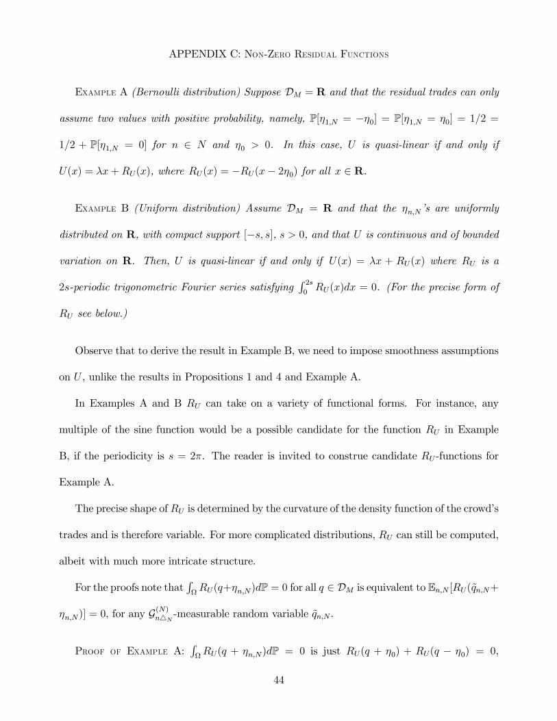
APPENDIX C: NON-ZERO RESIDUAL FUNCTIONS

EXAMPLE A (Bernoulli distribution) Suppose DM = R and that the residual trades can only

assume two values with positive probability, namely, P[η1,N = −η0] = P[η1,N = η0] = 1/2 =

1/2 + P[η1,N = 0] for n ∈ N and η0 > 0. In this case, U is quasi-linear if and only if

U(x) = λx+RU(x), where RU(x) = −RU(x− 2η0) for all x ∈ R.

EXAMPLE B (Uniform distribution) Assume DM = R and that the ηn,N s are uniformly

distributed on R, with compact support [−s, s], s > 0, and that U is continuous and of bounded

variation on R. Then, U is quasi-linear if and only if U(x) = λx + RU(x) where RU is a

2s-periodic trigonometric Fourier series satisfyingR 2s0RU(x)dx = 0. (For the precise form of

RU see below.)

Observe that to derive the result in Example B, we need to impose smoothness assumptions

on U , unlike the results in Propositions 1 and 4 and Example A.

In Examples A and B RU can take on a variety of functional forms. For instance, any

multiple of the sine function would be a possible candidate for the function RU in Example

B, if the periodicity is s = 2π. The reader is invited to construe candidate RU -functions for

Example A.

The precise shape of RU is determined by the curvature of the density function of the crowds

trades and is therefore variable. For more complicated distributions, RU can still be computed,

albeit with much more intricate structure.

For the proofs note thatRΩRU(q+ηn,N)dP = 0 for all q ∈ DM is equivalent to En,N [RU(qn,N+

ηn,N)] = 0, for any G(N)n4N-measurable random variable qn,N .

PROOF OF EXAMPLE A:RΩRU(q + ηn,N)dP = 0 is just RU(q + η0) + RU(q − η0) = 0,

44

q ∈ R. Q.E.D.

PROOF OF EXAMPLE B: Under the assumption that U is quasi-linear, equation (6) becomes

(15)Z q+s

q−sRU(x)dx = 0 for all q ∈ R.

By differentiating the above integral equation with respect to q, we obtain thatRU is 2s-periodic

on R. Since, by assumption, RU is continuous and of bounded variation, it has a trigonometric

Fourier representation given by

(16) RU(q) =∞Xn=1

han cos(

πn

sq) + bn sin(

πn

sq)i,

an =1

s

Z s

−sRU(x) cos(

πn

sx)dx, bn =

1

s

Z s

−sRU(x) sin(

πn

sx)dx.

The above Fourier series does not have an intercept part, a0, since a0 =R s−sRU(x)dx = 0.

Hence RU possesses the claimed 2s-periodic trigonometric Fourier series withR 2s0RU(x)dx = 0.

Conversely, if RU(q) = U(q) − λq is 2s-periodic and satisÞesR 2s0RU(x)dx = 0, then it has

the representation (16) and meets (15). Q.E.D.

45

REFERENCES

ALLEN, F., AND D. GALE (1992): Stock-Price Manipulation, Review of Financial Studies, 5,

503-529.

AMIHUD, Y., AND H. MENDELSON (1980): Dealership Market: Market-Making with

Inventory, Journal of Financial Economics, 8, 31-53.

BERNARDO, A. E., AND O. LEDOIT (2000): Gain, Loss, and Asset Pricing, Journal of

Political Economy, 108, 144-172.

BERTSIMAS, D., AND A. W. LO (1998): Optimal Control of Execution Costs, Journal of

Financial Markets 1, 1-50.

BLACK, F. (1995): Equilibrium Exchanges, Financial Analysts Journal, May-June, 23-29.

BREEN, W. J., L. HODRICK, AND R. A. KORAJCZYK (2002): Prediciting Equity Liquidity,

Management Science, 48, 470-483.

CHAN, L. K., AND J. LAKONISHOK (1995): The Behavior of Stock Prices around Institutional

Trades, Journal of Finance, 50, 1147-1174.

CHEN, Z., W. STANZL, AND M. WATANABE (2002): Price-Impact Costs and the Limit of

Arbitrage, Unpublished Manuscript, Yale University.

COCHRANE, J. H., AND J. SAA-REQUEJO (2000): Beyond Arbitrage: Good-Deal Asset Price

Bounds in Incomplete Markets, Journal of Political Economy, 108, 79-119.

DUTTA, P. K., AND A. MADHAVAN (1995): Price Continuity Rules and Insider Trading,

Journal of Financial and Quantitative Analysis, 30, 199-221.

DYBVIG, P. H., AND S. A. ROSS (1987): Arbitrage, in The New Palgrave: Finance, ed. by J.

Eatwell, M. Milgate, and P. Newman, MacMillan Press, New York, 57-71.

EASLEY, D., AND M. OHARA (1987): Price, Trade Size, and Information in Securities

46

Markets, Journal of Financial Economics, 19, 69-90.

(1992), Time and the Process of Security Price Adjustment, Journal of Finance, 47,

577-605.

GEMMILL, G. (1996): Transparency and Liquidity: A Study of Block Trades on the London

Stock Exchange under Different Publication Rules, Journal of Finance, 51, 1765-1790.

GLOSTEN, L. R., AND P. MILGROM (1985): Bid, Ask, and Transaction Prices in a Specialist

Market with Heterogeneously Informed Agents, Journal of Financial Economics, 14,

71-100.

HASBROUCK, J. (1991): Measuring the Information Content of Stock Trades, Journal of

Finance, 46, 179-207.

HASBROUCK, J., AND T. HO (1987): Order Arrival, Quote Behavior, and the Return Generating

Process, Journal of Finance, 42, 1035-1048.

HAUSMAN, J. A., A. W. LO, AND A. C. MACKINLAY (1992): An Ordered Probit Analysis of

Transaction Stock Prices, Journal of Financial Economics, 31, 319-379.

HO, T., AND H. R. STOLL (1981): Optimal Dealer Pricing Under Transactions and Return

Uncertainty, Journal of Financial Economics, 9, 47-73.

HOLTHAUSEN, R., R. LEFTWICH, AND D. MAYERS (1987): The Effect of Large Block

Transactions on Security Prices, Journal of Financial Economics, 19, 237-267.

(1990): Large Block Transactions, the Speed of Response, and Temporary and

Permanent Stock-Prices Effects, Journal of Financial Economics, 26, 71-95.

HUBERMAN, G. (1982): A Simple Approach to Arbitrage Pricing Theory, Journal of

Economic Theory, 28, 183-191.

HUBERMAN, G., AND W. STANZL (2002): Optimal Liquidity Trading, Unpublished

47

Manuscript, Columbia University.

JARROW, R. A. (1992): Market Manipulation, Bubbles, Corners, and Short Squeezes,

Journal of Financial and Quantitative Analysis, 27, 311-336.

KEIM, D. B., AND A. MADHAVAN (1996): The Upstairs Market for Large Block Transactions:

Analysis and Measurement of Price Effects, Review of Financial Studies, 9, 1-36.

KEMPF, A., AND O. KORN (1999): Market Depth and Order Size, Journal of Financial

Markets, 2, 29-48.

KYLE, A. S. (1985): Continuous Auctions and Insider Trading, Econometrica, 53,

1315-1336.

LEDOIT, O. (1995): Essays on Risk and Return in the Stock Market, Ph.D. dissertation, MIT.

MADHAVAN, A., M. RICHARDSON, AND M. ROMMANS (1997): Why Do Security Prices Change?

A Transaction-Level Analysis of NYSE Stocks, Review of Financial Studies, 10,

1035-1064.

MERTON, R. C. (1990): Continuous-time Finance, Blackwell, Cambridge, MA, & Oxford, UK.

SCHOLES, M. S. (1972): The Market for Securities: Substitution versus Price Pressure and the

Effects of Information on Share Prices, Journal of Business, 45, 179-211.

48

FOOTNOTES

1We are grateful to Prajit Dutta, Charles Jones, and Matthew Rhodes-Kropf for conver-

sations and comments. Larry Glosten was especially and extremely helpful and supportive.

We also thank the participants of the NASDAQ-Notre Dame Conference 2000, the Western

Finance Association Meetings 2001, the European Finance Association Meetings 2001, and of

the ESSFM Meetings 2001 in Gerzensee; in particular, Craig Holden, Eugene Kandel, Mark

Loewenstein, Massimo Massa, and Anna Pavlova. An earlier version of this paper circulated

under the title Arbitrage-free Price-Update and Price-Impact Functions.

49

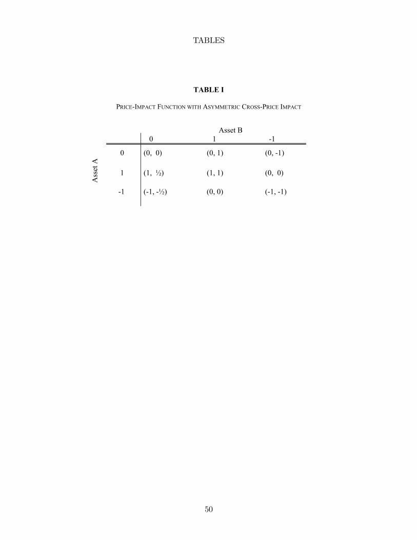
TABLES

TABLE I

PRICE-IMPACT FUNCTION WITH ASYMMETRIC CROSS-PRICE IMPACT

Asset B 0 1 -1

0 (0, 0) (0, 1) (0, -1)

1 (1, ½) (1, 1) (0, 0)

Ass

et A

-1 (-1, -½) (0, 0) (-1, -1)

50

LIST OF SYMBOLS

1. Model related:

4N , pn,N , pn,N , qn,N , qn,N , Pn,N , Un,N , εn,N , ηn,N ,

Pn,N , Un,N , P , U, Uij , q0,N , q0,Nm , VP , VU ,

T (q0,N), π(q0,N), SR(q0,N), GLR[z], RU , qj∞j=1, c(.),

Ω, F , P, E, V ar, Std, En,N , F (N)n4N

, G(N)n4N,

DM , Dη, Dε, D, DjM , M1(4N), M1, M2, M∗1,

λn,N , µn,N , ε−1,N , z+, z−, u, σ2ε, σ2η, ΛN , Λj,N ,

α, λ, η, Na(q,n), X, Y.

2. Parameters & Constants:

θ, θm, δ, q, v, n, N, N0, Nm, x, τ , K,

i, j, π, nm, n0m, η0, a0, ε, N .

3. Sets:

N, Q, R, R+, L(R), C.

4. Operators:

≡, ⊆, ∝, 6=, R, ∓, ∩, ∞, ∈, ↓, ↑, →,

F [f ], O(g),PN

n=1,P∞

n=1,RΩ,

RR,

R ba,

√x, sin,

cos, max, min, sup, inf, argmax, arg sup, lim, det.

51