TABLE 8.13. Summary of Single Number Risk Measure and Risk Indices

Risk measure Value

Maximum individual risk 2.4 x 10~5 / yr

Average individual risk

Exposed population 8.8 X 1(T6 / yr

Total population 7.5 x 1O-6 / yr

Fatal accident rate 0.10 fatalities / 108 man-hr exposure

Average rate of death 2.1 X 10~3 fatalities / yr

Equivalent social cost

Okrent 3.5 x 1(T3

Netherlands 2.7 x 10~2

FAR is normally used to measure risk to on-site personnel. If we assume thatthe populated area represents an occupied part of the plant, and that the peopleare present at all times, then the FAR can be calculated for this example.

FAR = (8.8 x lO^yr1) (1.14 x 104)= 0.10 fatalities / 108 exposure hours

Table 8.13 summarizes the various single number measures of risk and riskindices calculated for this example.

8.1.7. Conclusions

This case study illustrates a simple CPQRA using a representative set of incidents tocalculate risk for a simplified chlorine rail tank car loading facility. Both individual andsocietal risk measure are estimated and presented. These can be compared with com-pany or other risk targets. Alternatively, risk reduction measures that would reduce theconsequences of incidents or the frequency of occurrence, as well as more fundamentaldesign parameters such as facility location, can all be evaluated quantitatively. The cost-benefit for each option can be developed and rational basis ensured for consideration ofrisk reduction measures.

8.2. Distillation Column

8.2.1. Introduction

This second case study addresses the risks associated with a system containing flamma-ble materials. The depth of study for this case (Figure 8.9) represents an intermediatelevel of complexity using a representative set of incidents in the risk plane.

Previous Page

FIGURE 8.9. Depth of study for Case Study 8.2.

The first case study (Section 8.1) used HAZOP to identify potential incidents. Asimple neutral buoyancy model was used for dispersion, the historical record and faulttree analysis were used for frequency estimation, and individual and societal risks forrisk estimation. This case study demonstrates a different depth of study using othertechniques. Incidents are identified by assuming only basic line and vessel failures, andtheir frequencies are estimated from the historical record. External events and dominoeffects are not included to simplify the analysis in this example. Resulting vapor cloudreleases are modeled using a heavy gas dispersion model. Various fire and explosionincident outcomes are developed via event tree analysis and examined using variousconsequence models considering both overpressure and thermal radiation effects. Asingle weather condition and a nonuniform 8-point wind rose reduce the number ofincident outcome cases. The result is an estimate for both individual risk and societalrisk to a neighboring community.

8.2.2. Description

As in the example in Section 8.1, the facility in this example has been greatly simplifiedso that the risk analysis calculations can be illustrated in a reasonable amount of space inthis book. The facility as described does not necessarily represent a current or best prac-tice design for such a facility. In particular, it is not likely that such a facility would belocated so near a large population concentration. However, to illustrate the use of fireand explosion models in a quantitative risk analysis, the example has been set up with alarge population near the facility. Similarly, the process operating conditions and otherparameters have been set up for the purpose of illustrating risk calculations and should

Depth of studyfor Example 8.2

BoundingGroup

RepresentativeSet

ExpansiveList

ORiQiN

Simple

Intermediate

Complex

RISK ESTIMATION TECHNIQUE.Consequence Frequency Risk

NUMB

EROF

SELE

CTED

INCIDE

NTS

not be considered to represent real operating conditions for such a process. As in Section8.1, this example considers only a few potential incidents to allow the example to beexplained in a limited amount of space. The list of incidents described should not be con-strued to represent a complete list of incidents characterizing the risk of a real facility.

A C6 distillation column is used to separate hexane and heptane from a feed streamconsisting of 58% (wt) hexane and 42% (wt) heptane. The overhead condenser,thermosyphon reboiler, and accumulator are all included in this study. A line diagramof the column and associated equipment showing flow rates and line sizes is given inFigure 8.10.

The column operating pressure is 4 barg and the temperature range is 130-16O0Cfrom the top to the bottom of the column, respectively. The column bottoms andreboiler inventory is 6000 kg (13,228 Ib, roughly 6 min holdup) and there are about10,000 kg (22,046 Ib) of liquid on the trays. The condenser is assumed to have noliquid holdup and the accumulator drum inventory is 12,000 kg (26,455 Ib, roughly12 min holdup of feed rate). The material in the bottom of the column is approximately90% heptane and 10% hexane. The relevant physical properties for these materials aregiven in Table 8.14.

The plant site layout is presented in Figure 8.11. This is an old plant, and, to theeast, 80 m away, is an on site office and warehouse complex containing 200 people(present 24 hours a day), distributed uniformly on 1 ha (100 X 100 m) of land. Theremaining area around the site consists of open fields.

The study objective is to estimate the risk to the office/warehouse complex fromthe fractionation system from both individual and societal risk perspectives.

Pressure Relief Header 30 *&* 0.50 m ID

Piping Diameter Total Length

0.10m 10m0.15m 15m

0.50 m 25 m

FIGURE 8.10. The column and associated equipment.

Heptane 6.7 kg/s

Hexane 10 kg/s

Pump 2

Accumulator

Cold WaterOverhead Condenser

Column

4 Barg

Pump 1SteamReboiler18O0C8 Barg

Feed 16.7 kg/s

TABLE 8.14. Physical Properties3

Physical Properties Hcxanc Heptane

Boiling point (0C) 69 99

Molecular weight 86 100

Upper flammable limit (vol %) 7.5 7.0

Lower flammable limit (vol %) 1.2 1.0

Heat of combustion (J/kg) 4.5 x 107 4.5 x 107

Ratio of specific heats, £ 1.063 1.054

Liquid density at boiling point (kg/m3) 615 614

Heat of vaporization at boiling point (J/kg) 3.4 x 105 3.2 x 105

Liquid heat capacity (JAg-0K) 2.4 x 1Q3 2.8 X IQ3

"from DIPPR Handbook (AIChE, 1987)

In order to limit the number of calculations, only one average weather condition isconsidered—a wind speed of 1.5 m/s and F stability—representing a worst case weathercondition with a reasonable probability of occurrence. A more thorough risk estima-tion would include a number of different meteorological conditions, chosen to repre-sent the full spectrum of those recorded at the site. The consequence of using the worstcase weather condition is that risk results will be conservative with respect to frequency.

Area with200 People

FIGURE 8.11. The plant layout and surroundings.

DistillationColumn

Plan

t Bou

ndar

y

Scale

FIGURE 8.12. The wind rose for Case Study 8.2.

Figure 8.12 depicts the wind rose used in this example, which gives the probabilityof wind from each of eight directions.

8.2.3. Identification, Enumeration, and Selection of Incidents

One method of defining an initial list of incidents is to consider all possible breaks orruptures of items of equipment which would lead to a loss of containment. This InitialList can then be modified in a number of ways to produce a revised list. In this casestudy, special problems such as polymerization, corrosion, blockage, overpressuriza-tion, etc., are not considered.

Each line or vessel, of course, may break or rupture in an infinite number of ways.For example, a pipe break may be any size from a pinhole to a full bore rupture and maybe any position between the pipe ends. This spectrum of incidents needs to be reducedto a representative set of incidents as defined in the depth of study. In this example,possible pipe failures are represented by either full bore ruptures or holes 20% of thepipe diameter. Minor localized incidents (e.g., flange leaks, pump seal leaks) by them-selves are not capable of causing long distance effects, but could result in a pool fire.The diking around the column limits the pool size to 10 m2. The rule of thumb that"safe" radiation fluxes (4.7 kW/m2) would exist at distances of between 3 and 5 timesthe pool diameter would suggest that a pool fire would not threaten the office/ware-house complex. However, if a separate study were to be conducted for risks to in-plantemployees, this incident might be considered.

The risk analyst should consider, in this example, incident outcomes such as firesand explosions since the material is flammable. Releases caused by different incidentsmay lead to similar incident outcomes and these can be combined to reduce the

calculational burden. The final choice of incidents to be modeled is a difficult onerequiring judgment from the analyst, but the following factors are taken intoconsideration:

• the size of the release• whether the release is instantaneous or continuous• whether the release is liquid or vapor

The final choice of incident outcomes to be modeled is also difficult and is usuallydetermined after screening consequence-calculations are performed. For flammablereleases, the possibility of both immediate and delayed ignitions should be considered.

The revised list of incidents chosen is

1. Complete rupture• column• accumulator• reboiler• condenser

2. Liquid leaks (full bore rupture and hole equivalent to 20% of diameter)• column feed line• reboiler feed line• heptane pump (Pump 2) suction line (including flanges and pump)• heptane pump (Pump 2) discharge line (including flanges)• condenser discharge line• reflux pump (Pumpl) suction line (including flanges and pump)• reflux pump (Pump 1) discharge line (including flanges)• shell leak (of column, accumulator, reboiler or condenser) of hole size equiva-

lent to 20% of pipe diameter only3. Vapor leaks (full bore rupture and hole equivalent to 20% of diameter)

• column overhead line• reboiler discharge line• shell leakage (of the column, accumulator, reboiler or condenser) of• hole size equivalent to 20% of pipe diameter only

While manageable with computer analysis, this list of incidents is too long formanual calculation. The list contains many incidents that would have similar or identi-cal incident outcomes, and this set can be reduced to the Representative Set of incidentsthrough the following assumptions, and judgment:

1. There are no automatic isolation valves within this system. However, it isassumed that automatic isolation exists at the system boundaries such that noadditional fuel other than what is present in the system at the time of the inci-dent contributes to the release. Therefore, an instantaneous failure of one vesselwill lead to the rapid release of the entire contents of all other connected vessels.

In addition the discharge from the relief valve is connected to a pressurerelief header. Reverse flow through the relief valve-due to back pressure duringany of the release scenarios-that might contribute additional release is assumednot credible.

2. All liquid lines have diameter of either 0.10 or 0.15 m. For simplicity all theliquid lines are assumed to have a diameter of 0.15 m. A quick estimate of thedischarge rate can be used to establish whether the full bore rupture of theselines can be treated as a instantaneous or continuous release. To estimate thedischarge rate from a catastrophic break in the liquid piping, it is consideredappropriate to use a liquid discharge model rather than a two-phase dischargemodel. Releases close to the vessel are well approximated by the liquid model,and release in piping using a liquid discharge model will be conservative. Amore detailed study might distinguish between several release locations andemploy more rigorous modeling for each.

The discharge equation for the continuous liquid releases from the 0.15 mdiameter line is [Eq. (2.1.15)]

I fg p \m=pvA = pACDl2 \-?-L + ghL (2.1.15)

V V P I

wheremL = mass discharge rate (kg/s)p = liquid density (615 kg/m3)v — fluid velocity (length/time)A = hole cross-sectional area (for 0.15 m dia, 1.77 X 10"2 m2)C0 = discharge coefficient (for liquids use 0.61) (dimensionless)gc = gravitational constantPg = upstream pressure(400 kPa gauge)g = acceleration due to gravity (9.8 m/s2)bL = liquid head (assume O m)

From this equation, the discharge rate for the liquid release from one end of thepipe is 239 kg/s. It is possible that the flow rate could be double this value if thepipe broke such that flow was unimpeded from both ends.

At this initial rate, the entire contents of the column, reboiler, and accumu-lator would be lost in 2 minutes. In practice it would take somewhat longer asthe pressure in the system would decrease during the release. Therefore, it isconsidered reasonable to treat full bore ruptures of liquid lines the same as a cat-astrophic failure of any vessel in the fractionating system.

3. Both vapor lines are 0.5 m in diameter. Again, a quick estimate of the dischargerate can be used to establish whether the full bore rupture of these lines can betreated as an instantaneous or continuous release.

To estimate the actual discharge rate from a catastrophic break in the gaspiping, first a calculation should be performed to determine if the flow is sonic.

From Eq. (2.1.18)

r**« (J_}k/(t-l} (2.L18)P1 (* + iJ

wherePchoked = maximum downstream pressure resulting in maximum flow

P1 = upstream pressure (5.01 bar abs)

P2 = downstream pressure (1.01 bar abs, atmospheric)k = heat capacity ratio (1.063 for hexane, 1.054 for heptane).The upstream pressure is 5.01 bar resulting in a choked pressure ofPMe4 =

(5.01 bar)(2.96) = 14.8 bar. The discharge downstream is to atmosphericpressure which is less than the calculated choked flow, thus sonic flow isexpected.

The equation for sonic or choked flow is given by

\kg M( 2 V4+1"'*-" (2.1-17)^choked- C0^-P1 j-^r- 1J

where^choked = §as discharge rate, choked flow (kg/s)

C0 = discharge coefficient (approximately 1.0 for gases)A = hole cross-section area (for 0.5 m dia pipe, 0.196 m2)

P1 = upstream pressure (5.01 X 105 N/m2 absolute)M = Molecular weight (kg/kg-mol) (86 for hexane, 100 for heptane)R - Gas constant (8314 J/kg-mole/°K)T = upstream temperature (hexane 4030K, heptane 4330K)

The vapor discharge rate is 309 kg/s for pure hexane and 321 kg/s for pureheptane.

Therefore, full-bore ruptures of vapor lines are also treated the same as acatastrophic failure of any vessel in the fractionating system.

The above assumptions produce the following representative set of inci-dents:

A. a catastrophic failure of the column, reboiler, condenser, accumulator, orany full bore liquid or vapor line rupture

B. liquid release through a hole of diameter equal to 20% of a 0.15 m diameterline

C. a vapor release through a hole of diameter equal to 20% of a 0.5m diameterline

These incidents include one very large, but rare release (Incident A, a catastrophicfailure of a vessel or full bore rupture) and two moderate release cases (Incidents B andC). The derivation of incident outcomes for Incidents A, B, and C will be carried outlater with the aid of event trees.

8.2.4. Incident Consequence Estimation

8.2.4.1 FLASH, DISCHARGE AND DISPERSION CALCULATIONS(INCIDENTS A, B AND C)

Flash discharge and dispersion calculations for Incidents A, B, and C defined above arecarried out using the methods described in Section 2.1.2.

Incident A: Catastrophic Failure. In the event of catastrophic failure of one of thevessels or a full bore line rupture, it is assumed that the entire contents of the column,reboiler, condenser, and accumulator are lost instantaneously. In the following calcula-tion, the flash fraction is determined assuming the column reboiler and accumulator con-tain pure heptane and pure hexane, respectively, rather than mixtures [Eq. (2.1.36)].

(T-rb)^ 7 V=Cp- (2.1.36)

whereFv = fraction of liquid flashed to vaporCp = average liquid heat capacity over the range T to Tb (2400 J/kg 0K for

hexane, 2800 J/kg 0K for heptane)T = initial temperature (13O0C for hexane, 16O0C for heptane)Tb = final temperature or atmospheric boiling point (690C for hexane,

990C for heptane)hfg = heat of vaporization (3.4 X 105 J/kg for hexane, 3.2 X 105 J/kg for heptane)The calculated flash fractions are 0.43 for hexane and 0.53 for heptane. Therefore,

both of these materials exhibit a flash fraction roughly 0.5. It is reasonable to assumefrom the discussion in Section 2.1.2 that all the hexane and heptane released will releasea gas and aerosol. It is further assumed that the aerosol droplets are small enough toremain suspended and evaporate instead of raining out onto the ground.

At the release conditions, both hexane and heptane are significantly denser thanair, with relative densities of 2.0 and 2.3 respectively. As the releases are relatively large,the dispersion of the instantaneous release defined above is calculated using a densecloud model. The top hat model of Cox and Carpenter as incorporated in theWHAZAN software program is used to determine the dispersion of the release forwind speed of 1.5 m/s and F stability. Although WHAZAN was used for this problemother software programs employing a dense gas model could have been used.

The thermophysical properties of hexane and heptane are similar. For this casestudy it was decided to base the dispersion calculations on hexane which comprisesapproximately two-thirds of the inventory of the system. The definition of the sourceterms for the instantaneous release and the atmospheric conditions assumed are givenin Table 8.15 and discussed below.

Since the release should consist only of gas and aerosol droplets that eventually evap-orate into the cloud, an all gaseous release is the option chosen for the dispersion analysis.

The temperature used is 690C, which is the temperature to which hexane liquidwill flash when released to the atmosphere.

It is necessary to estimate the initial dilution, which is the number of volumes of aircontaining one volume of gas in the could after expansion to atmospheric pressure andbefore heat transfer and dispersion processes begin. A value of 10 was chosen based ona suggested dilution range of 10:1 to 100:1 by Kaiser and Walker (1978) from empiri-cal evidence and photographs of specific incidents.

The initial cloud radius is set equal to the cloud height, which is the most commondefault for top-hat models.

The results of the calculations are shown in Table 8.16. The puff formed by theinstantaneous release could reach a centerline concentration of 1.2% at a distance ofapproximately 85 m, which is just inside the office/warehouse complex.

TABLE 8.15. Data Used for Instantaneous Heavy Gas DispersionCalculations

Quantity Instantaneous release

Mass released 28,000 kg

Release rate —

Temperature 690C

Dilution factor 10

Cloud radius Equal to height

Atmospheric stability Stable (F)

Wind speed 1.5 m/s

Surface roughness parameter O. lm

Ambient temperature 2O0C

Ambient humidity 80%

TABLE 8.16. Results of Dispersion Calculations for the Instantaneous Release(Incident A)

Distance Center-line Clouddownwind Cloud radius Cloud height concentration temperature

Time(s) (m) (m) (m) (vol %) (0K)

O O 32 32 7.8* 309

20 30 91 14 2.2 297

40 60 125 11 1.5 296

57 85 148 9.5 1.2 295

The initial concentration is calculated for a 10 times dilution of hot hexane into ambient air.On mixing, the air will work, the hexane will cool, and the total volume of the cloud will increase.This results in an initial concentration of 7.8% (vol).

Incidents B and C: Liquid and Vapor Release from Hole in Piping. For a liquidrelease, the flash fraction is the same as for Incident A. An identical assumption is madethat the entire release is a gas and aerosol cloud, with no liquid rainout.

The discharge rate for the liquid release (Incident B) can be estimated using Eq.(2.1.15), assuming a hole diameter of 0.03 m. The resulting discharge rate is 9.6 kg/s.The discharge rate for the gaseous release (Incident C) can be estimated using Eq.(2.1.17), assuming a hole diameter of 0.10 m. The calculated discharge rate is 12.4 kg/s.

For simplicity, since both release are assumed to be gaseous and the discharge ratesare similar, Incidents B and C are combined into one representative average release ofvapor with a flow rate of 11 kg/s.

These releases are expected to provide a continuous release of material over anextended time period. Again, the top hat dense cloud model incorporated intoWHAZAN is used to determine the dispersion of the release, Table 8.17 presents thedata used in the source terms and Table 8.18 presents the results of the calculation.

The flammability zone from the continuous release will extend into theoffice/warehouse complex.

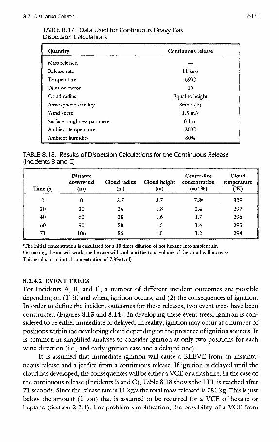
TABLE 8.17. Data Used for Continuous Heavy GasDispersion Calculations

Quantity Continuous release

Mass released —

Release rate 11 kg/s

Temperature 690C

Dilution factor 10

Cloud radius Equal to height

Atmospheric stability Stable (F)

Wind speed 1.5 m/s

Surface roughness parameter 0.1 m

Ambient temperature 2O0C

Ambient humidity 80%

TABLE 8.18. Results of Dispersion Calculations for the Continuous Release(Incidents B and C)

Distance Center-line Clouddownwind Cloud radius Cloud height concentration temperature

Time(s) (m) (m) (m) (vol %) (0K)

O O 3.7 3.7 7.8" 309

20 30 24 1.8 2.4 297

40 60 38 1.6 1.7 296

60 90 50 1.5 1.4 295

71 106 56 1.5 1.2 294

aThe initial concentration is calculated for a 10 times dilution of hot hexane into ambient air.On mixing, the air will work, the hexane will cool, and the total volume of the cloud will increase.This results in an initial concentration of 7.8% (vol)

8.2.4.2 EVENTTREESFor Incidents A, B, and C, a number of different incident outcomes are possibledepending on (1) if, and when, ignition occurs, and (2) the consequences of ignition.In order to define the incident outcomes for these releases, two event trees have beenconstructed (Figures 8.13 and 8.14). In developing these event trees, ignition is con-sidered to be either immediate or delayed. In reality, ignition may occur at a number ofpositions within the developing cloud depending on the presence of ignition sources. Itis common in simplified analyses to consider ignition at only two positions for eachwind direction (i.e., and early ignition case and a delayed one).

It is assumed that immediate ignition will cause a BLEVE from an instanta-neous release and a jet fire from a continuous release. If ignition is delayed until thecloud has developed, the consequences will be either a VCE or a flash fire. In the case ofthe continuous release (Incidents B and C), Table 8.18 shows the LFL is reached after71 seconds. Since the release rate is 11 kg/s the total mass released is 781 kg. This is justbelow the amount (1 ton) that is assumed to be required for a VCE of hexane orheptane (Section 2.2.1). For problem simplification, the possibility of a VCE from

FIGURE 8.14. Event tree for Incidents B and C.

Incidents B and C is ignored in this analysis, and the only outcome considered is a flashfire. A more complex study could include the possibility of a VCE.

If a vessel fails catastrophically with no ignition, it is possible for the stored PVenergy to produce a shock wave and present a threat based on overpressure alone. Thisparticular consequence is not considered in the analysis. Projectiles may also be pro-duced by a catastrophic rupture of a vessel, but the risk from these is assumed negligiblerelative to effects of fire and explosion.

From the event trees, the following incident outcomes are identified for the riskanalysis:

• BLEVE due to immediate ignition of and instantaneous release• VCE due to delayed ignition of an instantaneous release

BLEVE•{Incidentoutcome 1)

UVCE•(Incidentoutcome 2)

Flash fire{Incidentoutcome 3)

Noconsequences

Jet fire'(Incidentoutcome 4)

Rash fire{Incidentoutcome 5)

Noconsequences

ignition

FIGURE 8.13. Event tree for Incident A.

Immediate ignition

Continuousrelease

Delayedignition

Noignition

No immediateignition

Instantaneousrelease

Immediate ignition

No immediateignition

Delayedignition

Conditionsfavor UVCE

Conditions favorflash fire

• flash fire due to delayed ignition of an instantaneous release• jet fire from immediate ignition of a continuous release• flash fire due to delayed ignition of a continuous release

8.2.4.3. CONSEQUENCES OF INCIDENT OUTCOMESThe consequences of the incident outcomes are calculated using the methods describedin Section 2.2. For this example, flammable effects are defined using a discrete effectzone approach, within which all people are assumed to be fatalities and outside ofwhich all people are assumed to be nonfatalities. This method overestimates the pro-portion of fatalities within the zone and underestimates them beyond it. The zones offatal effect for the various incident outcomes are calculated as follows:

Incident Outcome No. 1: BLEVE due to Immediate Ignition of an Instanta-neous Release. For a BLEVE involving 28,000 kg of hexane (M) the followingparameters are calculated using a proprietary software package:

• peak BLEVE diameter 181 m• BLEVE duration 12 s• center height of BLEVE 136 m

As discussed earlier, some of the release cases included in the BLEVE incident out-come involve releasing the 28,000 kg inventory over a period greater than the 12 sec-onds calculated here (e.g., full bore rupture of piping) and would probably not result ina classical BLEVE. This means that the BLEVE consequences are overestimated.

For a duration of 12 seconds, the incident radiation required for fatality of an aver-age individual is approximately 75 kW/m2. This is derived from Figure 2.95 for the50% fatality line at 12 seconds.

The incident radiation from a BLEVE is given by Eq. (2.2.45):

Et =r,EF2l (2.2.45)where

Er = incident radiationra = transmissivityE = surface emitted flux (kW/m2)P21= view factor

the transmissivity is given by Eq. (2.2.42)

ra =2.02(Pw*s)-°-09 (2.2.42)

where Pw is the water partial pressure at ambient conditions (N/m2) and x is the pathlength between flame surface and receiver (m).

The path length x is calculated as

* = V(H*LEVE+rV^ = V(1362+r2)-90.5

where r is the horizontal distance from the column to the receiver.Assuming that Pw = 2810 N/m2 (Sample Problem Section 2.28), Eq. (2.2.42)

reduces to

r=0.99[(1362 +r 2 ) 0 ' 5 -90.S]'0'09

Using Eq. (2.2.47) withD = Dmax:

T7 __^MAX

**—&-

hence

P21 = 819Or-2

And from an energy balance on the emitted energy [Eq. (2.2.4O)]

RMH,h = ^

71^MAX ^BLEVE

R = 0.25 and the heat of combustion for hexane is 4.5 X 10~7 J/kg. Therefore, E =255 kW/m2. This value may be entered into the expanded equation (2.2.42):

£>R =|0.99[(Vl362 + r2)-90.5] ° J(255)(8190r-2)

For a radiation level Q^ °f 75 kW/m2, this equation may be solved by iteration togive r— 135m. Therefore, the area of fatal effect is a circle of radius 135 m, centered onthe column, which would extend into the office/warehouse complex.

Incident Outcome No. 2: Unconfined Vapor Cloud Explosion due to DelayedIgnition of Instantaneous Release. This incident outcome involves 28,000 kg ofhexane. Using the TNT equivalent model (Section 2.2.1.2) the equivalent mass ofTNT is given by Eq. (2.2.1).

W=TjM —^cTNT

whereW = equivalent mass of TNT (kg)M = actual mass of hydrocarbon (28,000 kg)

r\ = empirical explosion yield (assumed to be 0.1)Ec = heat of combustion of hydrocarbon (4.5 x 107 J/kg for hexane)

^CTNT = heat of combustion of TNT (4.6 X 106 J/kg)Hence, the equivalent mass of TNT is 27,391 kg (60,387 Ib).

The use of an empirical explosion yield of 0.1 should represent a reasonable worstcase result for an explosion incident outcome.

An overpressure of 3 psi is used to calculate the extent of fatal effects (Section2.3.3.2). From a figure equivalent to Figure 2.48 but in English units [Figure 2.18 inthe 1989 edition of this book (CCPS, 1989)] the scaled range (Z0) for an overpressureof 3 psi is 15 ft/lb1/3. To convert this to an actual distance,

RG = ZGWl/* = 15 x 60,3781/3 = 588 ft (179 m)

Hence, the area of fatal effect for a VCE of 28,000 kg of hexane is a circle of radius179 m, centered 85 m downwind or the column, which would extend well into theoffice/warehouse complex.

Incident Outcome No. 3: Flash Fire due to Delayed Ignition of an InstantaneousRelease. For flash fires, and approximate estimate for the extent of the fatal effect zoneis the area over which the cloud is above the LFL. It is assumed that this area is notincreased by cloud expansion during burning. This is a circular zone of 148 m radiuscentered 85 m downwind (Table 8.16).

Incident Outcome No. 4: Jet fire from Immediate Ignition of a ContinuousRelease. Very rough calculation using the simplified method of Considine and Grint(1984), although strictly application to LPG, yields an end hazard range of 50% lethalityat 31 m for a 100-s exposure. This result suggests that there is no direction threat to theoffice/warehouse complex and this incident outcome is not considered further.

Incident Outcome No. 5: Flash Fire due to Delayed Ignition of a ContinuousRelease. The area over which the cloud formed by the continuous release is above theLFL can be derived from Table 8.18. This gives a pie-shaped hazard zone 162 m longdownwind (106 m distance + 56 m radius) with 64° of arc [i.e., 2 tan~1(56 /(1062 -56Y)].

This incident can impact the office/warehouse complex and is considered further inthis study.

The net result of these consequence effect calculations is that four other IncidentOutcomes (Nos. 1, 2, 3, and 5) could impact the office/warehouse complex.

The next step in the calculation procedure is to determine Incident and IncidentOutcome frequencies.

8.2.5. Incident Frequency Estimation

8.2.5.1. FREQUENCIES OF THE REPRESENTATIVE SET OF INCIDENTSFor this example, data from the historical record (Section 3.1) have been used in orderto estimate the frequencies of the Representative Set of incidents. This method is appli-cable to cases where the items considered are similar in design to those for which his-torical record of failure rates exists. In this case the column, vessels, pipes, and pumpsare standard process equipment and historical failure rate data are available for suchitems (e.g., Rijmnond Public Authority, 1982).

The basic failure rate data are listed in Table 8.19. For each item of equipment, thefrequencies of a number of different sizes of failure are given. These are quoted per itemyear except for piping for which frequencies are given per meter-year.

Using Table 8.19 and the numbers of vessels, pumps, and pipe lengths included inthe representative set of incidents, the frequencies are calculated as follows:

Incident A: Instantaneous Release. This incident includes the following failures:

• catastrophic rupture of any component in the fractionating system• catastrophic (full bore) rupture of any pipework

There is approximately 25 m of 0.5 m diameter piping and 25 m of 0.15 m equiva-lent diameter piping included in this incident. Hence, the frequency is calculated asfollows:

TABLE 8.19 Example Failure Frequency (for Illustration Purposes)

Item Size of failure Failure rate

Piping

Small < 50 mm dia. Full bore rupture 8.8 X 10~7 (m yr'1)

20% of pipe dia. rupture 8.8 x 10~7 (m yr1)

Medium > 50 mm dia. Full bore rupture 2.6 X 10~7 (m yr"1)

< 150 mm dia. 20% of pipe dia. rupture 5.3 x 10"6 (m yr"1)

Large > 150 mm dia. Full bore rupture 8.8 x 10~8 (m yr""1)

20% of pipe dia. rupture 2.6 x 10"6 (m yr"1)

Fractionating system Serious leakage 1.0 X 10~5 (m yr"1)(excluding piping) Catastrophic rupture 6.5 X IQ"6 (m yr"1)

• Catastrophic rupture offractionating system: 6.5 x 10"6 = 6.5 x 10"6 yr"1

• Full bore of55 m of medium pipe 25 x 2.6 x 10~7 = 6.5 x 1(T6 yr"1

25 m of large pipe 25 x 8.8 x 10~8 = 2.2 x 1(T6 yr"1

• Total 1.5 x IQ-5 yr"1

Incidents B and C: Continuous Release. This incident includes holes of 20% of thediameter for all piping, and serious leakage form vessels. There are approximately 25 mof large 0.5 m diameter piping and 25 m of medium 0.15 m diameter piping includedin this incident. Hence, the frequency is calculated as follows:

• Leaks from55 m of medium pipe 25 x 5.3 x 10"6 = 1.3 x 10"4 yr1

25 m of large pipe 25 x 2.6 x 10"6 = 6.5 x 10"5 yr"1

• Serious leakage fromfractionating system 1.0 X 10"5 = 1.0 X 10"5 yr"1

•Total 2.1 x 10"4Vr"1

8.2.5.2. PROBABILITIES OF INCIDENT OUTCOMESThe probability of each incident outcome is determined by assigning probabilities to allof the branches of the event trees of Figures 8.13 and 8.14. Some of the probabilitiesare direction dependent (i.e., the proportion of the office/warehouse complex involvedaffects the probability of ignition). For this case study, two event trees have been devel-oped for each incident-one that considers wind directions toward the office/warehousecomplex and one that considers all other directions. The results of this exercise areshown in Figures 8.15 through 8.18. For this case study, the branch probabilities forthese event tree have been derived using engineering judgment. In a real risk assess-ment, better validated sources would be preferred. It is important that such assump-tions are documented for later review and sensitivity analysis if warranted. A summaryof the values selected and their justification is listed in Tables 8.21 and 8.22.

FIGURE 8.16. Event tree for Incident A,instantaneous release; wind from all other directions(directions away from residential area).

8.2.5.3. PREPARATION OF INCIDENT OUTCOME CASE FREQUENCIESThe prior analysis of a revised list of potential incidents (under the categories of com-plete rupture, liquid leaks and vapor leaks) gives a representative set of three potentialincidents (Incidents A5 B5 and C). It is assumed that with minimal loss in accuracy,those incidents can be characterized as a single catastrophic incident (Incident A) andsingle continuous release (Incidents B and C). The event tree analysis developed theinstantaneous and continuous release incidents to four specific incident outcomes that

FIGURE 8.15. Event tree for Incident A, instantaneous release; wind from SW, W. and NWdirections (directions affecting residential area).

BLEVE(Incident

"outcome 1)p «0.25

UVCEIncident

"outcome 2)p -0.34

Flash fire(Incident

"outcome 3)p m 0.34

No-consequencep - 0.08

BLEVE.(Incidentoutcome 1)p-0.25UVCE(Incident

'outcome 2)p -0.08

Rash fire(Incident"outcome 3)p - 0.08

No-consequencep - 0.60

Instantaneousrelease

Instantaneousrelease

Delayedignitionp -0.2

No immediateignitionp - 0.75

Immediate ignitionp -0.25

Immediate ignitionp - 0.25

No immediateignitionp - 0.75

Delayedignitionp -0.9

Flash firep -0.5

Noignitionp -0.1

Noignitionp -0.8

FIGURE 8.18. Event tree for Incidents B and C continuous release; wind from all otherdirections (directions away from residential area).

TABLE 8.20. Incident Outcomes Impacting the Residential Area

Incidentoutcomenumber Incident outcome

1 BLEVE due to immediate ignition of an instantaneous release

2 UVCE due to delayed ignition of instantaneous release

3 Flash Fire due to delayed ignition of an instantaneous release

5 Flash Fire due to delayed ignition of continuos release

FIGURE 8.17. Event tree for Incidents B and C continuous release; wind from SW, W. andNW directions (directions affecting residential area).

Jet fire (no.threat to public)p -0.1

Flash fire,(Incidentoutcome 5)p - 0.68

No-consequencep - 0.22

Jet fire (no.threat to public)p -0.1

Flash fire,(Incident"outcome 5)p m 0.09

No-consequencep - 0.81

Continuousrelease

Continuousrelease

Immediate ignitionp -0.1

Delayedignitionp - 0.75

No immediateignitionp -0.9

|Joignitionp -0.25

Delayedignitionp -0.1

No immediateignitionp -0.9

IJo __ignitionp -0.9

Immediate ignitionp -0.1

TABLE 8.21 . Event Tree Branch Probabilities — Instantaneous Releasefrom Figures 8. 1 5 and 8. 1 6

Branch

Immediate ignition (BLEVE)

No immediate ignition

Delayed ignition[From Figure 8.15 (windfrom SW, W & NW)]

No ignition

UVCE

Flash Fire

Delayed ignition[From Figure 8.16 (windfrom all other directions)

No ignition

Branch number

1

2

3A

4A

5

6

Probability

0.25

0.75

0.9

0.1

0.5

0.5

Basis

Cause for failure may be fire andthe release will initially extend toa wide area

Ignition likely due to large size ofcloud and the presence ofpopulation resulting in largernumber of ignition sources

High likelihood of UVCEbecause the release is a very largequantity of flashing liquid

Lower likelihood of ignition dueto smaller number of ignitionsources

TABLE 8.22. Event Tree Probabilities — Continuous Releasefrom Figures 8. 1 7 and 8. 1 8

Branch

Immediate ignition

No immediate ignition

Delayed ignition[From figure 8.17 (windfrom SW, W & NW)]

No ignition

Delayed ignition[From figure 8.18 (windfrom all other directions)]

No ignition

Branch number

7

8

9A

1OA

9B

1OB

Probability

0.1

0.9

0.75

0.25

0.1

0.9

Basis

Low likelihood of immediateignition due to lack of localignition sources and low rateof release

High likelihood of delayedignition due to presence ofpopulation

Low likelihood of delayedignition due to smaller numberof ignition sources

can impact the office/warehouse complex. A summary of the incident outcomes islisted in Table 8.22.

The frequencies of incident outcome cases, which are dependent on wind direc-tion, are calculated in Table 8.23. In that table the headings are defined as:

Incident: The incident from the representative set chosen for the analysis

Incident outcome: The incident outcomes related to a particular incident which wereshown to have potential for public impact

Incident frequency: The frequency of each incident in the representative set

Incident outcome probability: The probability of an incident outcome based onevent tree analysis given that the probability of the incident is 1.0

Incident outcome frequency: The product of the incident frequency and the incidentoutcome probability

Directional probability: The probability of the wind blowing in a particular directionbased on the wind rose

Incident outcome case frequency: The product of the incident outcome frequencyand the directional probability

TABLE 8.23. Frequencies of Incident Outcome Cases

IncidentIncident Incident Incident outcome case

Incident frequency outcome outcome Directional frequencyIncident outcome (y*~l) probability* frequency From probability' (y*'1)

A 1 BLEVE 1.5 x IQ-5 0.25 3.8 x IQ-6 — — — 3.8 x IQ-6

A 2 VCE 1.5 x 10-5 0.34 5.1 x IQ-6 SW NE 0.20 1.0 x IQ-*

0.34 5.1 x HH W E 0.15 7.7 x 10~7

0.34 5.1 x 1(H NW SE 0.10 5.1 x 10~7

0.08 1.2 x HH N S 0.10 1.2 x 10~7

0.08 1.2 x 10-6 NE SW 0.10 1.2 x 10~7

0.08 1.2 x HH E W 0.10 1.2 x 10~7

0.08 1.2 x 10-6 SE NW 0.10 1.2 x 10~7

0.08 1.2 x KH S N 0.15 1.8 x 10~7

A 3 1.5 x 10-5 0.34 5.1 x IQ-6 SW NE 0.20 1.0 x IQ-6

FlashFire 0.34 5 . IxIO- 6 W E 0.15 7.7 x 10~7

0.34 5.1 x 10-6 NW SE 0.10 5.1 x 10~7

0.08 1.2 x KH N S 0.10 1.2 x 10~7

0.08 1.2 x 10-6 NE SW 0.10 1.2 x 10~7

0.08 1.2 x 10-6 E W 0.10 1.2 x 10~7

0.08 1.2 x 10-6 SE NW 0.10 1.2 x 10~7

0.08 1.2 x 10-6 s N 0.15 1.8 x 10~7

B & C 5 2.1 x 1(H 0.68 1.4 x IQ-4 SW NE 0.20 2.9 x IQ-5

0.68 1.4 x 10-4 W E 0.15 2.1 x 10~5

0.68 1.4 x 1(H NW SE 0.10 1.4 x 10~5

0.09 1.9 x 10-5 N S 0.10 1.9 x IQ-6

0.09 1.9 x IO-5 NE SW 0.10 1.9 x IQ-6

0.09 1.9 x 10-5 E W 0.10 1.9 x 10

0.09 1.9 x 10-5 SE NW 0.10 1.9 x IQ-6

0.09 1.9 x IO-5 S N 0.15 2.9 x IQ-6

"From Figures 8.15-8.18.frFrom Figure 8.12.

8.2.6. Risk Estimation

8.2.6.1. INDIVIDUALRISKThe individual risk in the area around the column is estimated from the above incidentoutcome case frequencies and consequence effect zones. The discrete consequenceeffect zones were estimated previously.

Incident Outcome1. BLEVE A circle of radius 135 m centered on the column.2. VCE A circle of radius 179 m centered 85 m from the column.3. Flash Fire (Instantaneous) A circle of radius 148 m centered 85 m from the

column.5. Flash Fire (Continuous) A pie shaped section (64° angle) that extends a total

of 162 m from the column. The radius is 56 m centered on a point 106 m fromthe column.

These four consequence effect zones have been superimposed over the plant layoutto scale in the east direction in Figure 8.19. From consequence considerations only, the

FIGURE 8.19. The plant layout and surroundings.

Scale

DistillationColumn

2VCEInstantaneous(Delayed Ignition)

3 Flash FireInstantaneous(Delayed Ignition)

1 BLEVEInstantaneous(Immediate Ignition)

Plan

t Bou

ndar

y

5 Fl

ash

Fire

'

Con

tinuo

us(D

elay

ed Ig

ntio

n)

consequence effects, ranked in descending order, are VCE, flash fire (instantaneous),BLEVE, and flash fire (continuous).

The four consequences effects described above can be divided into 3 commontypes:

1. circular shaped, centered on column (Incident Outcome 1)2. circular shaped, centered 85 m from column (Incident Outcomes 2 and 3)3. pie shaped, originating at column (Incident Outcome 5)

Each of these must be treated slightly differently in calculating individual risk, butit is straightforward to extend this procedure to any effect zone shape and position.

Figures 8.20-8.23 illustrate the general shape of the individual risk profile as afunction of distance, for each of the four incident outcomes, along any wind direction

FIGURE 8.20. Risk profile for Incident outcome 1: BLEVE.

FIGURE 8.21. Risk profile for Incident outcome 2: VCE.

Distance (m) Risk contribution

0-94 All 8 directions94-108 7 directions

157-228 5 directions228-264 3 directions

> 264 O directions

RISK

RISK

FIGURE 8.23. Risk profile for incident outcome 5: flash fire (continuous).

(including the east direction that contains the office/warehouse complex). The zeropoint in each of the figures is the location of the fractionating system.

It is very important in the estimation of the individual risk (and as will be shownlater, in the estimation of societal risk) that overlapping incident be properly consid-ered. Thus, with the large VCE consequence effect zone, consideration of only the W

RISK

FIGURE 8.22. Risk profile for incident outcome 2: flash fire (instantaneous).

Distance (m) Risk contribution

0-63 All 8 directions63-75 7 directions

75-120 5 directions120-194 3 directions194-233 1 directions

> 233 O directions

RISK

to E wind case would greatly underestimate the risk of those living to the east of VCEincidents from all 8 directions contribute to the risk.

The calculation of individual risk at any point assumes that the contributions of allincident outcome cases are additive. Therefore, the total individual risk at each point isequal to the sum of the individual risks from all possible incident outcome cases.

The individual risk in this study is not symmetrical around the column because ofthe directional probabilities of the wind and ignition. Ideally, an individual risk con-tour could be developed that includes points in each of the eight wind directions. How-ever, in this study, the population is only situated east of the plant, and an individualrisk curve will be developed only for that easterly direction.

Each of Figures 8,20 to 8.23 contains a set of distances for that incident outcome.Each distance listed on a particular figure represents a subset of incident outcome casesthat reach that distance. However, other incident outcomes can also provide cases thatapply at that same distance. Therefore, for every distance listed in Figures 8.20 to 8.23a calculation should be made that sums all of the total incident outcome cases that con-tribute at that distance.

Table 8.24 presents a summation of the individual risk for a distance of 0-63 m inan easterly direction from the column. All incident outcome cases contribute in this cal-culation with the exception of flash fire (continuous) wind direction N to S, NE to SW,E to W, SE to NW, and S to N.

Table 8.25 has been developed to show the changes to total individual risk thatresult at each discrete distance. This permits development of the total individual riskcurve in the east direction (Figure 8.24).

TABLE 8.24 Estimation of Individual Risk

Incident Frequencies of Total frequencyoutcome incident outcome for each incident

Distance from Incident outcomes cases cases contributing outcome casecolumn (m) contributing contributing (yr'1) (y*~l)

0-63 1 BLEVE Wind 3.8 x 1(H 5.7 x IQ-6

directionindependent

2 UVCE SW to NE 1.6 x 1(H

NW to SE 1.2 x 1(H

N to S 1.8 x IO-7

NE to SW 1.8 x 10-7

E to W 1.8 x 10-7

SE to NW 1.8 x 10-7

S to N 2.8xlO-7 4 ,6XlO-6

3 Flash Fire (Inst.) Same as 2 4.6 x IQ-6

5 Flash Fire (Cont) SW to NE 5.0 x 10-5 1,1 x IQ-4

W to E 3.8x10-5

NW to SE 2.5 x 10-5

Total individual risk = 1,25 X IO"4 yr'1

TABLE 8.25. Total Individual Risk at Discrete Distances in the East Direction3

Distance segment (m)

At O up to 63

At 63 up to 75

At 75 up to 94

At 94 up to 108

At 108 up to 120

At 120 up to 135

At 135 up to 157

At 157 up to 162

At 162 up to 194

At 194 up to 228

At 228 up to 233

At 233 up to 264

>264

Incident outcome case thatno longer impact on the

total individual risk

Flash Fire (Cont.)

N to S

NE to SW

E to W

SE to NW

S to N

Flash Fire (Inst.)

E to W

Flash Fire (Inst.)

SE to NW

NE to SW

UCVE

E to W

UVCE

NE to SW

SE to NW

Flash Fire (Inst.)

N to S

S to N

Flash Fire (Cont.)

SW to NE

NW to SE

UVCE

N to S

S to N

Flash Fire (Cont.)

W to E

Flash Fire (Inst.)

SW to NE

NW to SE

UVCE

SW to NE

NW to SE

Flash Fire (Inst.)

Wto E

UVCE

W to E

Total individual risk (yr"1)

7.39 x IO-5

7.38 x 10-5

7.36 x 10-5

7.34 x 10-5

7.32 x 10-5

7.29 x IO-5

2.63 x 10-5

2.60 x 10-5

4.59 x 10-6

3.06 x 10-*

1.53 x 10-6

7.65 x 10-6

O

"From the data in this table, a curve for the total individual risk curve in the east direction can be developed, whichis shown in Figure 8.21.

DISTANCE TO EAST OF COLUMN (m)

FIGURE 8.24. Individual risk versus distance in the east direction.

Some observations on the results are

1. The risk near the column has probably been underestimated, since small inci-dents that may contribute to the risk in this area have been excluded form theanalysis (e.g., jet fire hazards).

2. The choice of only two places for ignition (immediate and delayed until theLFL concentration is reached) simplifies the real situation of ignition point atintermediate locations due to office/warehouse complex, fired process equip-ment, roads, etc. A different ignition distribution could be considered, but withincreased calculational burden.

3. The use of only one weather condition (F stability, 1.5 m/s wind speed) gener-ally tends to overestimate risk at a given distance, because the longest disper-

IND

IVID

UA

L R

ISK

OF

FAT

AL

ITY

(P

ER

YE

AR

)

sion distances are usually associated with F stability, low wind speedconditions.

4. The risk from VCE is probably overestimated because of the high explosiveyield chosen.

These assumptions have been chosen to provide a reasonable, but conservative,risk estimate using a minimum number of manual calculations. Where the resultingrisk estimates indicate a potential problem, the analyst can decide whether some simpli-fying assumptions should be made more realistic, and the calculations repeated. How-ever, each change in an assumption probably represents a significant increase in thenumber of incident outcome cases. An alternative approach is to use a computer toolthat automates the calculation procedure, allowing analysis of greater number of inci-dent outcome cases.

8.2.6.2. SOCIETALRISKThe first step in the estimation of societal risk is to calculate the number of fatalities foreach incident outcome case. For this case study, consequence effect zones are discrete(within the zone there will be 100% fatalities) and an assumption is made that the

TABLE 8.26. Estimation of Number of Fatalities for Each incident Outcome Case

Incident outcome case Estimated number ofIncident outcome case frequency (yr'1) fatalities

1 BLEVE 3.8 x 1(H 80

2VCE

SW to NE 1.0 XlO-6 200

W to E 7.7X10-7 150

NW to SE 5.IxIO-7 200N to S 1.2 x IO-7 I30

NE to SW 1.2x10-7 80

E to W 1.2X10-7 80

SE to NW 1.2x10-7 80

S to N 1.8x10-7 130

3 Flash Fire (Inst.)

SW to NE 1.0 x IO-6 130

W to E 7.7 x IO-7 150

NW to SE 5 . Ix IO- 7 130N to S 1.2 x IO-7 40

NE to SW 1.2x10-7 O

E to W 1.2x10-7 O

SE to NW 1.2x10-7 O

S to N 1.8XlO-7 40

5 Flash Fire (Cont.)

SW to NE 2.9 x IO-5 5

W to E 2 . Ix IO- 5 40

NW to SE 1.4 x IO-5 5

office/warehouse complex has a uniform population distribution. Therefore, the frac-tion of office/warehouse complex covered by each incident outcome case will representthe fraction of 200 fatalities which would result. Table 8.26 summarizes these results.

The data in Table 8.26 represent the raw information from which the societal riskestimate may be developed. The data must be put into a cumulative frequency form inorder to plot the F-N curve. This is accomplished by rearranging the incident outcomecases by descending number of fatalities, and then calculating the frequency of havingN or more fatalities. This procedure is presented in Table 8.27.

The data in the first and last column are plotted on logarithmic scales to producethe F-N curve shown in Figure 8.25. Adding more incident outcome cases will pro-duce a smoother curve because of the additional data points, but will necessarily pro-duce significant upward or downward bias.

8.2.7. Conclusions

The largest contribution to individual risk near to the column is from flash fires frompipe rupture equivalent to 20% of the pipe diameter. Remedial measures might includemore frequent inspection or monitoring of wall thickness, if significant corrosionand/or erosion effects are anticipated.

The largest contributor to the societal risk, not unexpectedly, is from instanta-neous release of the contents and delayed ignition resulting in an unconfined vaporcloud explosion.

TABLE 8.27 Societal Risk Estimation

CumulativeIncident frequency of N

Number of outcome case or morefatalities Incident outcome case frequency (yr'1) fatalities (yr'1)

200 2 VCE SW to NE 1.0 x IQ-6 1.5 x HH

200 2 VCE NW to SE 5.1 x 10~7

150 2 VCE W to E 7.7 x 10~7 1.5 x 10"6

150 3 Flash Fire W to E 7.7 x 10~7

130 2 VCE S to N 1.8 x 10~7

130 2 VCE N to S 1.2 x 10~7

130 3 Flash Fire SW to NE 1.0 x IQ-6 1.8 x 10

130 3 Flash Fire NW to SE 5.1x 10~7

80 2 VCE NE to SW 1.2 x IQ-7

80 2 VCE SE to NW 1.2 x 10~7

80 2 VCE E to W 1.2 x 10~7 4.1 x IQ-6

80 1 BLEVE 3.8 x 10"6

40 5 Flash Fire W to E 2.1x IO'5

40 3 Flash Fire S to N 1.8 x 10~7 2.2 x 10'5

40 3 Flash Fire N to S 1.2 x 10~7

5 5 Flash Fire SW to NE 2.9 x 10~5 4.3 x IO'5

5 5 Flash Fire NW to SE 1.4 x 10~5

NUMBER OF FATALITIES (N)

FIGURE 8.25. Total societal risk from the fractionating system.

The radius of the consequence zone is proportional to the 1/3 power of the quan-tity released. Therefore, only a very major reduction in quantity has a significant effectin reducing that radius. Nonetheless, additional remote isolation for the system couldbe considered. Vessel and piping integrity is the major concern. Additional inspection,perhaps utilizing different methods, could be considered.

Finally, because of the magnitude of the societal risk, additional study could con-sider other causes of vessel failure, such as overpressurization, that could lead to identi-cal consequences. These studies, probably utilizing FTA, could indicate whether athreat of overpressurization is significantly higher than basic vessel failure, and engi-neering or procedural controls could be implemented to reduce that risk.

FRE

QU

EN

CY

OF

N O

R M

OR

E F

AT

AL

ITIE

S (P

ER

YE

AR

)

8.3. References

American Institute of Chemical Engineers (AIChE) (1987). DIPPR Handbook. New York:American Institute of Chemical Engineers.

Center for Chemical Process Safety (CCPS) (1985). Guidelines for Hazard Evaluation Procedures.New York: American Institute of Chemical Engineers.

Center for Chemical Process Safety (CCPS) (1989). Guidelines for Chemical Process QuantitativeRisk Analysis. New York: American Institute of Chemical Engineers.

Center for Chemical Process Safety (CCPS) (1992). Guidelines for Hazard Evaluation Procedures,2nd Edition with Worked Examples. New York: American Institute of Chemical Engineers.

Considine, M. and Grint, G. C. (1984). "Rapid Assessment of the Consequences of LPGReleases." Proceedings of the Gastech 84 LNG/LPG Conference. Nov. 6-9. Gastech Ltd.,Rickmansworth, UK, 1985, pp. 187-200.

Kaiser, G. D. and Walker, B. C. (1978). "Releases of Anhydrous Ammonia from PressurizedContainers-The Importance of Denser Than Air Mixtures." Atmosphere Environment 12,2289-2300.

McMullen, R. W. (1975). 'The Change of Concentration Standard Deviations with Distance."JAPCA 25(10, October), 1057

Rijnmond Public Authority (1982). A Risk Analysis of 6 Potentially Hazardous Industrial Objectivein the Rijnmond Area—A Pilot Study. D. Reidel, Dordrecht, The Netherlands and Boston,MA. (ISBN 90-277-1393-6).

Turner, D. B. (1970). Workbook of Atmospheric Dispersion Estimates. Cincinnati, OH: U.S.Department of Health, Education, and Welfare.

Withers, R. M. J. and Lees, F. P. (1985). "The Assessment of Major Hazards: The Lethal Toxic-ity of Chlorine." (Parts 1 and 2}. Journal of Hazardous Materials 12 (3, December), 231-282and 283-302.