Preventing transition to turbulence using streamwise traveling waves:direct numerical simulations

Binh K. Lieu, Rashad Moarref, and Mihailo R. Jovanovic

Abstract— We use direct numerical simulations of the nonlin-ear Navier-Stokes (NS) equations to examine the effectivenessof streamwise traveling waves for controlling the onset ofturbulence in a channel flow. We highlight the effect of abase flow induced by the streamwise traveling waves on thedynamics of velocity fluctuations and on the net efficiencyof control. It is shown that properly designed downstreamtraveling waves are capable of reducing the fluctuations’ kineticenergy and maintaining the laminar flow. In contrast, ourresults demonstrate that upstream traveling waves promoteturbulence even when the uncontrolled flow stays laminar. Ournumerical simulations elucidate the predictive power of thetheoretical framework developed in a companion paper [1] andsuggest that the linearized NS equations with uncertainty serveas an effective control-oriented model for preventing transition.

Index Terms— Flow control; transition to turbulence; Navier-Stokes equations; direct numerical simulations; energy ampli-fication; skin-friction drag coefficient.

I. INTRODUCTION

Significant attention has recently been paid to the problemsof drag reduction and turbulence suppression in transi-tional and turbulent channel flows using sensorless controlstrategies. In this setup control action is formed withoutmeasurement of the relevant flow quantities and distur-bances, thereby circumventing estimation of velocity fluctua-tions based on noisy surface measurements (observer designin high-Reynolds-number flows is a challenging problem).In [2], it was shown by direct numerical simulations (DNS)that surface actuation in the form of an upstream travelingwave (UTW) can sustain sub-laminar skin-friction drag.

Currently available sensorless flow control strategies aredesigned using extensive numerical and experimental stud-ies. For example, an extensive number of simulations onturbulent drag reduction by means of spanwise wall oscil-lation was conducted in [3] where 37 cases of differentcontrol parameters were considered. Instead of an extensivenumerical study, this paper builds directly on the theoreticalfindings of a companion paper [1] where system-theoreticapproach was used to show that downstream traveling waves(DTWs) are capable of weakening the sensitivity to back-ground disturbances of the most energetic structures in a flowwith no control. The effectiveness of DTWs and UTWs inpreventing or enhancing transition is examined in this work.

B. K. Lieu, R. Moarref, and M. R. Jovanovic are with the Departmentof Electrical and Computer Engineering, University of Minnesota, Min-neapolis, MN 55455, USA (e-mails: lieux006@umn.edu, rashad@umn.edu,mihailo@umn.edu).

Financial support from the National Science Foundation under CAREERAward CMMI-06-44793 is gratefully acknowledged.

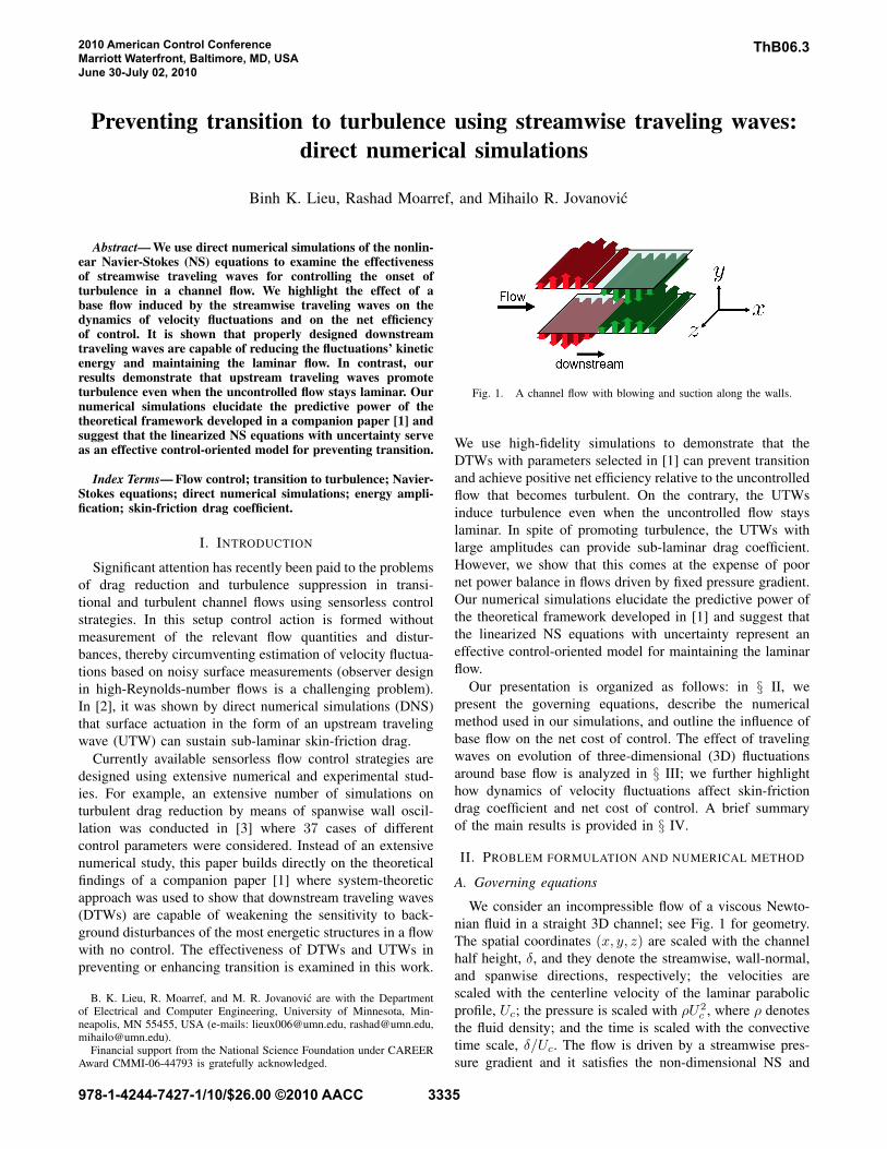
Fig. 1. A channel flow with blowing and suction along the walls.

We use high-fidelity simulations to demonstrate that theDTWs with parameters selected in [1] can prevent transitionand achieve positive net efficiency relative to the uncontrolledflow that becomes turbulent. On the contrary, the UTWsinduce turbulence even when the uncontrolled flow stayslaminar. In spite of promoting turbulence, the UTWs withlarge amplitudes can provide sub-laminar drag coefficient.However, we show that this comes at the expense of poornet power balance in flows driven by fixed pressure gradient.Our numerical simulations elucidate the predictive power ofthe theoretical framework developed in [1] and suggest thatthe linearized NS equations with uncertainty represent aneffective control-oriented model for maintaining the laminarflow.

Our presentation is organized as follows: in § II, wepresent the governing equations, describe the numericalmethod used in our simulations, and outline the influence ofbase flow on the net cost of control. The effect of travelingwaves on evolution of three-dimensional (3D) fluctuationsaround base flow is analyzed in § III; we further highlighthow dynamics of velocity fluctuations affect skin-frictiondrag coefficient and net cost of control. A brief summaryof the main results is provided in § IV.

II. PROBLEM FORMULATION AND NUMERICAL METHOD

A. Governing equations

We consider an incompressible flow of a viscous Newto-nian fluid in a straight 3D channel; see Fig. 1 for geometry.The spatial coordinates (x, y, z) are scaled with the channelhalf height, δ, and they denote the streamwise, wall-normal,and spanwise directions, respectively; the velocities arescaled with the centerline velocity of the laminar parabolicprofile, Uc; the pressure is scaled with ρU2

c , where ρ denotesthe fluid density; and the time is scaled with the convectivetime scale, δ/Uc. The flow is driven by a streamwise pres-sure gradient and it satisfies the non-dimensional NS and

2010 American Control ConferenceMarriott Waterfront, Baltimore, MD, USAJune 30-July 02, 2010

ThB06.3

978-1-4244-7427-1/10/$26.00 ©2010 AACC 3335

continuity equations

ut = − (u ·∇)u − ∇P + (1/Rc)∆u, 0 = ∇·u. (1)

Here, Rc denotes the Reynolds number, Rc = Ucδ/ν, ν isthe kinematic viscosity, u is the velocity vector, P is thepressure, ∇ is the gradient, and ∆ is the Laplacian, ∆ =∇ ·∇.

In addition to the constant pressure gradient, Px =−2/Rc, let the flow be subject to a zero-net-mass-fluxsurface blowing and suction in the form of a streamwisetraveling wave. The base velocity, ub = (U, V,W = 0),represents the steady-state solution to (1) in the presence ofthe following boundary conditions

V (y = ±1) = ∓2 α cos (ωx(x − c t)),U(±1) = Vy(±1) = W (±1) = 0,

(2)

where ωx, c, and α denote frequency, speed, and amplitudeof the traveling wave. Positive values of c define a DTW,while negative values of c define a UTW. In the presence ofvelocity fluctuations, u represents the sum of base velocity,ub, and velocity fluctuations, v = (u, v, w), where u, v, andw denote the fluctuations in the streamwise, wall-normal, andspanwise directions, respectively.

B. Numerical method

The traveling waves that are considered theoreticallyin [1] are tested in DNS of a 3D transitional chan-nel flow. All simulations performed in this work use thecode developed in [4]. A multi-step semi-implicit Adams-Bashforth/Backward-Differentiation (AB/BDE) scheme de-scribed in [5] is used for time discretization. The AB/BDEtreats the linear terms implicitly and the nonlinear termsexplicitly. A spectral method [6] is used for the spatialderivatives with Chebyshev polynomial expansion in thewall-normal direction and Fourier series expansion in thestreamwise and spanwise directions. Aliasing errors from theevaluation of the nonlinear terms are removed by the 3/2-rule when the horizontal FFTs are computed. We modifiedthe code to account for the boundary conditions (2).

The nonlinear NS equations are integrated in time with theobjective of computing the fluctuations’ kinetic energy andthe skin-friction drag coefficient, § III. The velocity fieldis first initialized with the laminar parabolic profile in theabsence of 3D fluctuations, § II-C; this yields the 2D baseflow which is induced by the fixed pressure gradient, Px =−2/Rc, and the boundary conditions (2). In simulationsof the full 3D flows (cf. § III), an initial 3D perturbationis superimposed to the base velocity, ub. As the initialperturbation, we consider a random velocity field which hasthe ability to trigger turbulence by exciting all the relevantFourier and Chebyshev modes [4]. This divergence-freeinitial condition is composed of random spectral coefficientsthat decay exponentially and satisfy homogenous Dirichletboundary conditions at the walls.

A fixed pressure gradient is enforced in all simulationswhich are initiated at Rc = 2000. We consider a stream-wise box length, Lx = 4π/ωx, for all controlled flow

simulations. This box length captures the streamwise modeskx = 0, ±ωx/2, ±ωx, ± 3ωx/2, . . .; relative to [1],these modes correspond to the union of the fundamental(kx = 0, ±ωx, ±2 ωx, . . .) and subharmonic (kx =±ωx/2, ± 3ωx/2, . . .) modes. In our presentation, in ad-dition to the uncontrolled flow, we consider two DTWs with(c = 5, ωx = 2, α = 0.035, 0.050), and three UTWswith (c = −2, ωx = 0.5, α = 0.015, 0.050, 0.125).The number of spatial grid points in x, y, and z directionsused in the uncontrolled and DTW flows are Nx = 50,Ny = 65, and Nz = 50, respectively; for the UTWs, weuse Nx = 200, Ny = 65, and Nz = 50. The total integrationtime is ttot = 1000 δ/Uc. We have verified our simulationsby making sure that the changes in results are negligibleby increasing the number of wall-normal grid points toNy = 97; we have also established agreement of our resultsfor UTWs with those of [2].

C. Base velocity and nominal net efficiency

The base velocity, ub = (U(x, y, t), V (x, y, t), 0), iscomputed using DNS of a 2D channel flow with Rc =2000 in the presence of streamwise traveling wave boundarycontrol (2). The nominal bulk flux is determined by UB,N =0.5

∫ 1

−1U(y) dy, where overline denotes the average over

horizontal directions. For the fixed pressure gradient, Px =−2/Rc, the nominal skin-friction drag coefficient is inverselyproportional to square of the nominal bulk, i.e., Cf,N =−2 Px/U2

B,N (cf. Table I). As shown in [7], compared tothe uncontrolled laminar flow, the nominal flux is decreased(increased) by DTWs (UTWs); this results in larger (smaller)nominal drag coefficients, respectively.

The above results suggest that upstream traveling wavescan exhibit increased flux compared to the uncontrolled flow.For the fixed pressure gradient, this results in production ofa driving power

Πprod = −Px (UB,c − UB,u) (2S),

where UB,c and UB,u denote the bulks of the controlledand uncontrolled flows, respectively, and S = LxLz is thearea of the wall. The normalized produced power %Πprod

is expressed as a percentage of the power spent to drive theuncontrolled flow, Πu = −Px UB,u (2S),

%Πprod = 100 (UB,c − UB,u) /UB,u.

On the other hand, the input power required for maintainingthe traveling waves is obtained from [8]

Πreq =(

V P∣∣y=−1

− V P∣∣y=1

)S,

and the normalized required power %Πreq is expressed as

%Πreq = 100V P

∣∣y=−1

− V P∣∣y=1

−2 Px UB,u.

In order to assess the efficacy of traveling waves for control-ling transitional flows, the control net power is defined as the

3336

Case c ωx α UB,N 103 Cf,N %Πprod %Πreq %Πnet

0 − − − 0.6667 4.5000 0 0 01 5 2 0.035 0.6428 4.8404 −3.58 16.64 −20.222 5 2 0.050 0.6215 5.1778 −6.77 31.74 −38.513 −2 0.5 0.015 0.6703 4.4513 2.70 5.46 −2.764 −2 0.5 0.050 0.7791 3.2949 16.86 37.69 −20.835 −2 0.5 0.125 1.0133 1.9478 51.99 145.05 −93.06

TABLE INOMINAL RESULTS IN CHANNEL FLOW WITH Rc = 2000. THE NOMINAL FLUX, UB,N , AND SKIN-FRICTION DRAG COEFFICIENT, Cf,N , ARE

COMPUTED IN THE 2D SIMULATIONS OF THE BASE FLOW DESCRIBED IN § II-C. THE PRODUCED POWER, %Πprod , REQUIRED POWER, %Πreq , AND

NET POWER, %Πnet , ARE NORMALIZED BY THE POWER REQUIRED TO DRIVE THE UNCONTROLLED FLOW. THE PRODUCED AND NET POWERS ARE

COMPUTED WITH RESPECT TO THE UNCONTROLLED LAMINAR FLOW.

difference between the produced and required powers [3]

%Πnet = %Πprod − %Πreq,

where %Πnet signifies how much net power is gained(positive %Πnet) or lost (negative %Πnet) in the controlledflow as a percentage of the power spent to drive the flowwith no control.

The nominal efficiency of the selected streamwise trav-eling waves in 2D flows, i.e. in the absence of velocityfluctuations, is shown in Table I. Note that the nominal netpower is negative for all controlled simulations. This is inagreement with a recent study of [7] where it was shownthat the net power required to drive a flow with transpiration-based control is always larger than in the (standard) pressuregradient type of actuation.

III. CONTROL OF TRANSITION BY TRAVELING WAVES

It was shown in [1] that a positive net efficiency can beachieved in a situation where the uncontrolled flow becomesturbulent but the controlled flow stays laminar. Whether thecontrolled flow can remain laminar depends on the dynamicsof velocity fluctuations around the modified base flow. In thissection, we study the influence of velocity fluctuations on thecontrol net efficiency in flows subject to streamwise travelingwaves. This problem is addressed by simulating full 3Dchannel flows in the presence of initial fluctuations which aresuperimposed on the base velocity. Depending on the kineticenergy of the initial condition, we distinguish two cases:(i) both the uncontrolled and properly designed controlledflows remain laminar (small initial energy); and (ii) theuncontrolled flow becomes turbulent, while the controlledflow stays laminar for the appropriate choice of travelingwave parameters (moderate initial energy). Our simulationsindicate, however, that poorly designed traveling waves canintroduce turbulence even for initial velocity fluctuations forwhich the uncontrolled flow stays laminar. It was demon-strated in [1] that properly designed DTWs are capable ofsignificantly weakening the intensity of velocity fluctuationswhich makes them well-suited for preventing transition;

on the other hand, compared to the uncontrolled flow, thevelocity fluctuations around the UTWs at best exhibit similarsensitivity to background disturbances.

The 3D simulations, which are summarized in Table II,confirm and complement the theoretical predictions in [1] attwo levels. At the level of transition control, we illustratein § III-A that the UTWs increase the intensity of velocityfluctuations and promote transition even for initial perturba-tions for which the uncontrolled flow stays laminar. In con-trast, the DTWs can prevent transition even in the presenceof initial conditions with moderate energy (cf. § III-B). At thelevel of net power efficiency, it is first shown in § III-A thatthe net power is negative when the uncontrolled flow stayslaminar. However, for the uncontrolled flow that becomesturbulent, we demonstrate that the DTWs that remain laminarcan result in a positive net efficiency. Our simulations in § III-B reveal that although UTWs become turbulent, a positive netefficiency can be achieved for small enough wave amplitudes.For the initial conditions with moderate energy, we furtherpoint out that the achievable positive net efficiency for UTWsis much smaller than for the DTWs that sustain the laminarflow (cf. § III-B).

A. Small initial energyWe first consider the initial fluctuations with small kinetic

energy, E(0) = 2.25×10−6, which cannot trigger turbulencein the uncontrolled flow. Our simulations show that theDTWs with parameters suggested in [1] improve transientresponse of the velocity fluctuations; on the contrary, theUTWs with parameters considered in [2] lead to deteriorationof the transient response and, consequently, enhance turbu-lence production. Since the uncontrolled flow stays laminar,both DTWs and UTWs lead to the negative net efficiency.

The energy of velocity fluctuations is given by

E(t) =1Ω

∫Ω

(u2 + v2 + w2) dΩ,

where Ω = 2S is the volume of the computational box.Fig. 2 shows the fluctuations’ kinetic energy as a functionof time for the uncontrolled and controlled flows. As evident

3337

Initial Energy Case c ωx α 103 Cf %Πprod %Πreq %Πnet

Small 0 − − − 4.5002 0 0 02 5 2 0.050 5.1778 −6.77 31.77 −38.543 −2 0.5 0.015 4.3204 −1.54 5.14 −3.604 −2 0.5 0.050 5.9426 −16.52 23.22 −39.745 −2 0.5 0.125 3.6853 12.20 108.41 −96.21

Moderate 0 − − − 10.3000 0 0 01 5 2 0.035 4.9244 52.07 26.44 25.632 5 2 0.050 5.2273 47.35 50.40 −3.053 −2 0.5 0.015 8.7866 11.36 4.53 6.834 −2 0.5 0.050 6.7406 31.15 41.96 −10.815 −2 0.5 0.125 3.9264 77.03 155.80 −78.77

TABLE IIRESULTS OF 3D SIMULATIONS IN CHANNEL FLOW WITH Rc = 2000. THE VALUES OF Cf , %Πprod , %Πreq , AND %Πnet CORRESPOND TO t = 1000.

FOR SMALL INITIAL ENERGY, THE PRODUCED AND NET POWERS ARE COMPUTED WITH RESPECT TO LAMINAR UNCONTROLLED FLOW; FOR

MODERATE INITIAL ENERGY, THEY ARE COMPUTED WITH RESPECT TO TURBULENT UNCONTROLLED FLOW.

from Fig. 2(a), the energy of the uncontrolled flow exhibitsa transient growth followed by an exponential decay tozero. We see that a DTW moves the transient responsepeak to a smaller time, which is about half the time atwhich peak of E(t) in the flow with no control takes place.Furthermore, maximal transient growth of the uncontrolledflow is reduced by approximately 2.5 times, and a muchfaster disappearance of the velocity fluctuations is achieved.On the other hand, Fig. 2(b) clearly exhibits the negativeinfluence of the UTWs on a transient response. In particular,the two UTWs with larger amplitudes (as selected in [2])significantly increase the energy of velocity fluctuations. Wenote that the fluctuations’ kinetic energy in a flow subjectto a UTW with an amplitude as small as α = 0.015 att = 1000 is already about two orders of magnitude largerthan the maximal transient growth of the uncontrolled flow.

Fig. 3(a) shows the skin-friction drag coefficient as afunction of time for the traveling waves considered in Fig. 2.The skin-friction drag coefficient is defined as [9]

Cf (t) =2τw

U2B

=1

Rc U2B

[(dU

dy+

du

dy

)∣∣∣∣y =−1

−(

dU

dy+

du

dy

)∣∣∣∣y = 1

],

(3)

where τw denotes the nondimensional average wall-shearstress and

UB(t) =12

∫ 1

−1

(U(y) + u(y, t)

)dy,

is the total bulk flux. Since both the uncontrolled flowand the flow subject to a DTW stay laminar, their dragcoefficients at the steady-state agree with the nominal valuescomputed in the absence of velocity fluctuations (cf. Tables I

(a) DOWNSTREAM (b) UPSTREAM

Fig. 2. Energy of the velocity fluctuations, E(t), for the initial conditionwith small energy: (a) ×, uncontrolled; , a DTW with (c = 5, ωx = 2,α = 0.05); and (b) UTWs with /, (c = −2, ωx = 0.5, α = 0.015);O, (c = −2, ωx = 0.5, α = 0.05); M, (c = −2, ωx = 0.5, α = 0.125).

and II). On the other hand, the drag coefficients of the UTWsthat become turbulent are about twice the values predictedusing the base flow analysis. The large growth of velocityfluctuations by UTWs has dramatically reduced the nominalflux and consequently increased the drag coefficients. Thevelocity fluctuations in the UTW with α = 0.015 are notamplified enough to have a pronounced effect on the dragcoefficient. Furthermore, the drag coefficients for the UTWswith (c = −2, ωx = 0.5, α = 0.05, 0.125) at t = 1000agree with the results of [2] computed for the fully developedchannel flow. This indicates that the UTWs with largeramplitudes in our simulations have transitioned to turbulence.The above results confirm the theoretical prediction of [1]where it is shown that the UTWs are poor candidates fortransition control for they enhance growth of the velocityfluctuations relative to the uncontrolled flow.

The net power as a function of time for the initial condi-tions with small kinetic energy are shown in Fig. 3. Note thatthe normalized net power for all traveling waves is negative

3338

(a) Cf (b) %Πnet

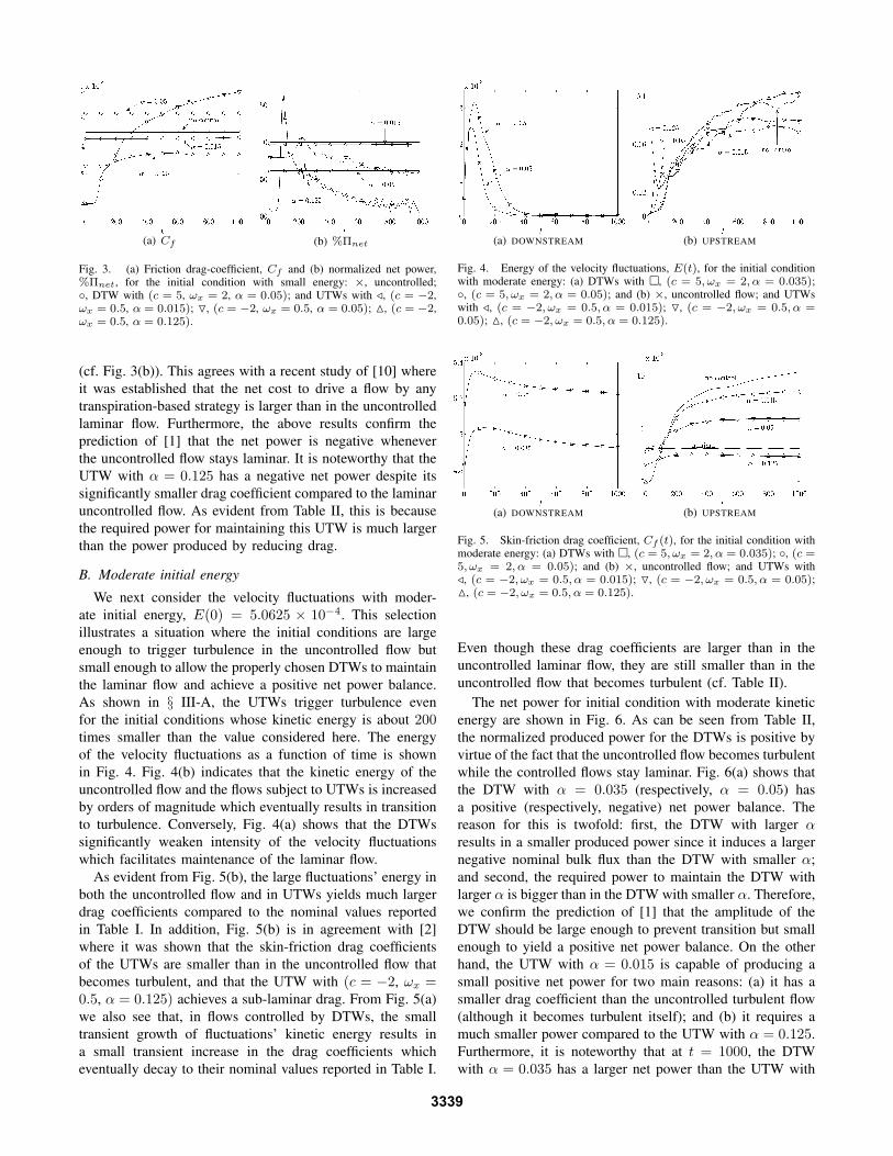
Fig. 3. (a) Friction drag-coefficient, Cf and (b) normalized net power,%Πnet, for the initial condition with small energy: ×, uncontrolled;, DTW with (c = 5, ωx = 2, α = 0.05); and UTWs with /, (c = −2,ωx = 0.5, α = 0.015); O, (c = −2, ωx = 0.5, α = 0.05); M, (c = −2,ωx = 0.5, α = 0.125).

(cf. Fig. 3(b)). This agrees with a recent study of [10] whereit was established that the net cost to drive a flow by anytranspiration-based strategy is larger than in the uncontrolledlaminar flow. Furthermore, the above results confirm theprediction of [1] that the net power is negative wheneverthe uncontrolled flow stays laminar. It is noteworthy that theUTW with α = 0.125 has a negative net power despite itssignificantly smaller drag coefficient compared to the laminaruncontrolled flow. As evident from Table II, this is becausethe required power for maintaining this UTW is much largerthan the power produced by reducing drag.

B. Moderate initial energy

We next consider the velocity fluctuations with moder-ate initial energy, E(0) = 5.0625 × 10−4. This selectionillustrates a situation where the initial conditions are largeenough to trigger turbulence in the uncontrolled flow butsmall enough to allow the properly chosen DTWs to maintainthe laminar flow and achieve a positive net power balance.As shown in § III-A, the UTWs trigger turbulence evenfor the initial conditions whose kinetic energy is about 200times smaller than the value considered here. The energyof the velocity fluctuations as a function of time is shownin Fig. 4. Fig. 4(b) indicates that the kinetic energy of theuncontrolled flow and the flows subject to UTWs is increasedby orders of magnitude which eventually results in transitionto turbulence. Conversely, Fig. 4(a) shows that the DTWssignificantly weaken intensity of the velocity fluctuationswhich facilitates maintenance of the laminar flow.

As evident from Fig. 5(b), the large fluctuations’ energy inboth the uncontrolled flow and in UTWs yields much largerdrag coefficients compared to the nominal values reportedin Table I. In addition, Fig. 5(b) is in agreement with [2]where it was shown that the skin-friction drag coefficientsof the UTWs are smaller than in the uncontrolled flow thatbecomes turbulent, and that the UTW with (c = −2, ωx =0.5, α = 0.125) achieves a sub-laminar drag. From Fig. 5(a)we also see that, in flows controlled by DTWs, the smalltransient growth of fluctuations’ kinetic energy results ina small transient increase in the drag coefficients whicheventually decay to their nominal values reported in Table I.

(a) DOWNSTREAM (b) UPSTREAM

Fig. 4. Energy of the velocity fluctuations, E(t), for the initial conditionwith moderate energy: (a) DTWs with , (c = 5, ωx = 2, α = 0.035);, (c = 5, ωx = 2, α = 0.05); and (b) ×, uncontrolled flow; and UTWswith /, (c = −2, ωx = 0.5, α = 0.015); O, (c = −2, ωx = 0.5, α =0.05); M, (c = −2, ωx = 0.5, α = 0.125).

(a) DOWNSTREAM (b) UPSTREAM

Fig. 5. Skin-friction drag coefficient, Cf (t), for the initial condition withmoderate energy: (a) DTWs with , (c = 5, ωx = 2, α = 0.035); , (c =5, ωx = 2, α = 0.05); and (b) ×, uncontrolled flow; and UTWs with/, (c = −2, ωx = 0.5, α = 0.015); O, (c = −2, ωx = 0.5, α = 0.05);M, (c = −2, ωx = 0.5, α = 0.125).

Even though these drag coefficients are larger than in theuncontrolled laminar flow, they are still smaller than in theuncontrolled flow that becomes turbulent (cf. Table II).

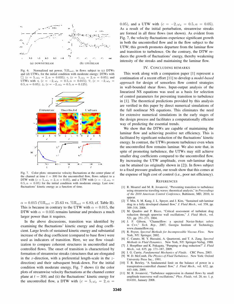
The net power for initial condition with moderate kineticenergy are shown in Fig. 6. As can be seen from Table II,the normalized produced power for the DTWs is positive byvirtue of the fact that the uncontrolled flow becomes turbulentwhile the controlled flows stay laminar. Fig. 6(a) shows thatthe DTW with α = 0.035 (respectively, α = 0.05) hasa positive (respectively, negative) net power balance. Thereason for this is twofold: first, the DTW with larger αresults in a smaller produced power since it induces a largernegative nominal bulk flux than the DTW with smaller α;and second, the required power to maintain the DTW withlarger α is bigger than in the DTW with smaller α. Therefore,we confirm the prediction of [1] that the amplitude of theDTW should be large enough to prevent transition but smallenough to yield a positive net power balance. On the otherhand, the UTW with α = 0.015 is capable of producing asmall positive net power for two main reasons: (a) it has asmaller drag coefficient than the uncontrolled turbulent flow(although it becomes turbulent itself); and (b) it requires amuch smaller power compared to the UTW with α = 0.125.Furthermore, it is noteworthy that at t = 1000, the DTWwith α = 0.035 has a larger net power than the UTW with

3339

(a) DOWNSTREAM (b) UPSTREAM

Fig. 6. Normalized net power, %Πnet, in flows subject to (c) DTWsand (d) UTWs, for the initial condition with moderate energy: DTWs with, (c = 5, ωx = 2, α = 0.035); , (c = 5, ωx = 2, α = 0.05); andUTWs with /, (c = −2, ωx = 0.5, α = 0.015); O, (c = −2, ωx =0.5, α = 0.05); M, (c = −2, ωx = 0.5, α = 0.125).

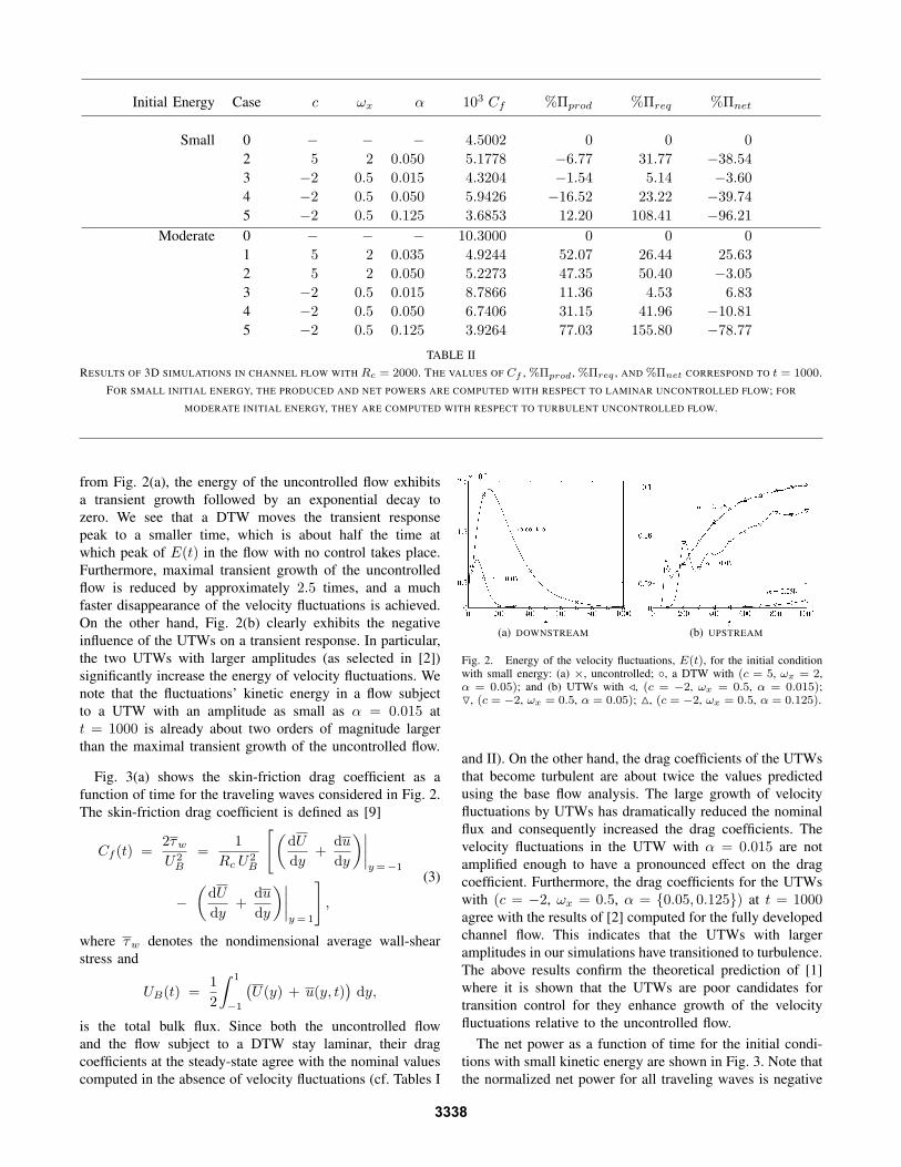
Fig. 7. Color plots: streamwise velocity fluctuations at the center plane ofthe channel at time t = 300 for the uncontrolled flow, flows subject to aDTW with (c = 5, ωx = 2, α = 0.05), and a UTW with (c = −2, ωx =0.5, α = 0.05) for the initial condition with moderate energy. Last row:fluctuations’ kinetic energy as a function of time.

α = 0.015 (%Πnet = 25.63 vs. %Πnet = 6.83; cf. Table II).This is because in contrary to the UTW with α = 0.015, theDTW with α = 0.035 remains laminar and produces a muchlarger power than it requires.

In the above discussions, transition was identified byexamining the fluctuations’ kinetic energy and drag coeffi-cient. Large levels of sustained kinetic energy and substantialincrease of the drag coefficient (compared to base flow) wereused as indicators of transition. Here, we use flow visual-ization to compare coherent structures in uncontrolled andcontrolled flows. The onset of transition is characterized byformation of streamwise streaks (structures that are elongatedin the x-direction, with a preferential length-scale in the z-direction) and their subsequent break-down. For the initialcondition with moderate energy, Fig. 7 shows (i) the colorplots of streamwise velocity fluctuations at the channel centerplane at t = 300; and (ii) the fluctuations’ kinetic energy forthe uncontrolled flow, a DTW with (c = 5, ωx = 2, α =

0.05), and a UTW with (c = −2, ωx = 0.5, α = 0.05).As a result of the initial perturbation, streamwise streaksare formed in all three flows (not shown). As evident fromFig. 7, the velocity fluctuations experience significant growthin both the uncontrolled flow and in the flow subject to theUTW; this growth promotes departure from the laminar flowand transition to turbulence. On the contrary, the DTW re-duces the growth of fluctuations’ energy, thereby weakeningintensity of the streaks and maintaining the laminar flow.

IV. CONCLUDING REMARKS

This work along with a companion paper [1] represent acontinuation of a recent effort [11] to develop a model-basedapproach for design of sensorless flow control strategiesin wall-bounded shear flows. Input-output analysis of thelinearized NS equations was used as a basis for selectionof control parameters for preventing transition to turbulencein [1]. The theoretical predictions provided by this analysisare verified in this paper by direct numerical simulations ofthe full nonlinear NS equations. This eliminates the needfor extensive numerical simulations in the early stages ofthe design process and facilitates a computationally efficientway of predicting the essential trends.

We show that the DTWs are capable of maintaining thelaminar flow and achieving positive net efficiency. This isfacilitated by significant reduction of the fluctuations’ kineticenergy. In contrast, the UTWs promote turbulence even whenthe uncontrolled flow remains laminar. We also note that, inspite of promoting turbulence, the UTWs may still achievesmaller drag coefficients compared to the uncontrolled flow.By increasing the UTW amplitude, even sub-laminar dragcan be attained (as originally shown in [2]). In flows subjectto a fixed pressure gradient, our result show that this comes atthe expense of high cost of control (i.e., poor net efficiency).

REFERENCES

[1] R. Moarref and M. R. Jovanovic, “Preventing transition to turbulenceusing streamwise traveling waves: theoretical analysis,” in Proceedingsof the 2010 American Control Conference, Baltimore, MD, 2010, toappear.

[2] T. Min, S. M. Kang, J. L. Speyer, and J. Kim, “Sustained sub-laminardrag in a fully developed channel flow,” J. Fluid Mech., vol. 558, pp.309–318, 2006.

[3] M. Quadrio and P. Ricco, “Critical assessment of turbulent dragreduction through spanwise wall oscillations,” J. Fluid Mech., vol.521, pp. 251–271, 2004.

[4] J. F. Gibson, “Channelflow: a spectral Navier-Stokes solverin C++,” Tech. Rep., 2007, Georgia Institute of Technology,www.channelflow.org.

[5] R. Peyret, Spectral Methods for Incompressible Viscous Flow. NewYork, NY: Springer, 2002.

[6] C. Canuto, M. Y. Hussaini, A. Quarteroni, and T. A. Zang, SpectralMethods in Fluid Dynamics. New York, NY: Springer-Verlag, 1988.

[7] J. Hoepffner and K. Fukagata, “Pumping or drag reduction?” J. FluidMech., vol. 635, pp. 171–187, 2009.

[8] I. G. Currie, Fundamental Mechanics of Fluids. CRC Press, 2003.[9] W. D. McComb, The Physics of Fluid Turbulence. New York: Oxford

University Press Inc., 1991.[10] T. R. Bewley, “A fundamental limit on the balance of power in a

transpiration-controlled channel flow,” J. Fluid Mech., vol. 632, pp.443–446, 2009.

[11] M. R. Jovanovic, “Turbulence suppression in channel flows by smallamplitude transverse wall oscillations,” Phys. Fluids, vol. 20, no. 1, p.014101, January 2008.

3340