The effect of wake turbulence intensity on transition in a compressor

cascade

Jan G. Wissink

School of Engineering and Design, Brunel University,

Uxbridge UB8 3PH, UK

and

Tamer A. Zaki

Department of Mechanical Engineering, Imperial College,

London SW7 2AZ, UK

and

Wolfgang Rodi

Institute for Hydromechanics, University of Karlsruhe,

Kaiserstr. 12, D-76128 Karlsruhe, Germany and

King Abdulaziz University, Jeddah, Saudi Arabia

and

Paul A. Durbin

Aerospace Engineering, Iowa State University,

Iowa, USA

Abstract

Direct numerical simulations of separating flow along a section at midspan of a low-pressure V103 compressor

cascade with periodically incoming wakes were performed. By varying the strength of the wake, its influence on

both boundary layer separation and bypass transition were examined. Due to the presence of small-scale three-

dimensional fluctuations in the wakes, the flow along the pressure surface was found to undergo bypass transition.

Only in the weak-wake case, the boundary layer was found to reach a nearly-separated state between impinging

wakes. In all simulations, the flow along the suction surface was found to separate. In the simulation with the strong

wakes, separation was found to be intermittently suppressed as the periodically passing wakes managed to trigger

turbulent spots upstream of the location of separation. As these turbulent spots were convected downstream, they

locally suppress separation.

1 Introduction

Low Pressure (LP) compressors typically consist of a large number of stages. The actual increase in pressure thatcan be realized in each stage is limited by the need to avoid massive boundary-layer separation which affects theaerodynamic performance of the blades and may cause structural damage. To some degree, separation is controlled byfree-stream fluctuations generated by the preceeding row of blades. To correctly predict the effects of impinging free-stream turbulence on the state of the blade’s boundary layer, advanced modelling strategies are needed. In engineeringapplications a variety of models are employed to predict the state of the boundary layer [9]. These range from crudealgebraic models to more complex and accurate models based on transport equations, as can be seen in [2, 10]. Toimprove existing models and to design new models for transition, data from both experiments and time-accuratenumerical simulations are needed.

Several experiments of flow in LP turbine cascades have been performed in the past [14, 15]. The accompanyingDNS-s [8, 18, 20, 21] allowed an even more detailed study of the physical mechanisms that drive boundary-layertransition in LP turbine blades. Relatively less effort has been dedicated to DNS of flow in compressor cascades.The present simulations are motivated by the experiments of flow in the LP V103A compressor cascade performedby Hilgenfeld and Pfitzner [6] who studied the combined effects of impinging wakes and background turbulence on

1

the development of the suction side boundary layer. It was found that the added effect of the periodically passingwakes on the blade’s boundary layer was largely masked by the overall effect of the uniformly distributed isotropicbackground turbulence. Hence, it was not possible to accurately analyse the influence of the periodically passing wakeson separation and transition of the compressor blade’s boundary layer.

Even though the available computational resources have increased significantly, a Direct Numerical Simulation(DNS) of the flow in realistic turbine or compressor stages is still far beyond the capabilities of modern supercomputers.The Reynolds number of such flows, however, is moderate, such that performing a DNS of flow for a simplified geometry- such as a two-dimensional section at midspan - is feasible. The first DNS-s of flow in a T106 turbine cascade withperiodically incoming wakes were performed by Wu and Durbin [21] and Wissink [18]. In both simulations, productionof fluctuating kinetic energy was observed at the apex of the deformed wake as it traveled through the passagebetween blades, and streamwise longitudinal vortical structures were found along the pressure side . These longitudinalstructures formed as the accelerating flow adjacent to the pressure side stretched the vortical structures in the wake,thereby aligning them with the direction of flow. Removing all fluctuations from the wake (see [20]) was found tobe sufficient to stop both the production of kinetic energy at the apex of the deformed wake and the formation oflongitudinal structures along the pressure side of the blade. While in the simulation by Wu and Durbin [21] the suctionside boundary layer was observed to undergo bypass transition, the larger inflow-angle employed in the simulationby Wissink [18] was found to lead to an intermittent separation of the boundary layer along the downstream half ofthe suction side. Kalitzin et al. [8] reported on a DNS of flow in the T106 turbine cascade with incoming free-streamturbulence (FST). Compared to the earlier DNS with incoming wakes by Wu and Durbin, the location of transitionof the suction side boundary layer was found to move further downstream. Because of the presence of high levels offree-stream fluctuations, the boundary layer flow on an LP turbine blade usually undergoes bypass transition.

The mechanism of bypass transition has been clarified by a number of studies of canonical boundary-layer flows,see e.g. [7, 24, 25, 11]). The mean-flow shear acts as a low-pass filter by only allowing low-frequency components ofthe free-stream turbulence into the boundary layer [26]. These penetrating disturbances cause the amplification ofelongated streaks, also known as Klebanoff modes. The streaks can reach amplitudes on the order of 10− 30% of thefree-stream speed, and some undergo a secondary instability that precedes the inception of localized turbulence spots[12]. The nature of the secondary instability depends on the flow configuration, for example the pressure gradient,and can be initiated near the edge of the boundary layer on close to the wall [17, 5]. Once formed, the turbulencespots grow as they are convected in the downstream direction, and finally merge into the fully-turbulent region.

Compared to the flow around an LP turbine blade, the boundary layer flow around an LP compressor blade ismore likely to separate and separation-induced transition is relatively common. Motivated by the experiments in theV103 compressor cascade [6], where it was found that the effect of the periodically impinging wakes on boundary layertransition was masked by the high intensity of the incoming background turbulence, a series of DNS-s of flow in aV103 compressor cascade was performed [22]. In these simulations the effect of FST alone (without wakes) on theblade’s boundary layer was studied. In the presence of FST, the boundary layer on the pressure side was found toremain attached due to transition to turbulence upstream of the location of separation in the laminar case. Alongthe suction surface, the separation was found to persist even at high levels of FST. By varying the levels of the FST,a rich variety of transitional mechanisms was found along the suction surface . At moderate levels of disturbances,two-dimensional waves could be identified and their development was still influenced by Klebanoff streaks due to thefree-stream forcing. For high levels of free-stream disturbances, the transition mechanism was found to shift towardsa pure bypass transition scenario.

Zaki et al. [27] studied the influence of periodically incoming weak wakes on transition and compared the flowto calculations without any inflow disturbances. On the pressure surface, the wakes were found to fully suppressseparation by periodically triggering bypass transition somewhat downstream of the leading edge. On the suctionsurface, only a periodic reduction in the size of the separation bubble was observed. The detached boundary layerwas found to roll up owing to a KH instability. Inside the rolls, the production of turbulent kinetic energy resultedin the formation of a turbulent wake-like flow downstream of the separation bubble, parallel to the suction surface. Itremained unclear, however, whether a stronger wake turbulence intensity can indeed suppress separation entirely or,perhaps, intermittently in the case of a strong adverse pressure gradient in the compressor passage. Whether this isthe case will be examined herein using direct numerical simulations.

One study relevant to this issue is the work by Coull and Hodson [3], although they focused on the pressuredistribution typical for the suction surface of a turbine blade, where the pressure gradient is locally adverse. Theyperformed experiments of boundary layer transition on a flat plate. The curvature of the top wall induced a varyingstreamwise pressure gradient along the plate that closely resembles the situation on the suction side of a high-liftLP turbine blade. The varying pressure gradient resulted in boundary-layer separation in the absence of free-stream

2

disturbances. A detailed study was performed of how FST and periodically passing wakes affect boundary-layertansition and separation. The grid-generated FST was found to induce weak Klebanoff streaks that, together withthe KH instability of the separated boundary layer, were found to promote transition. The addition of periodicallypassing wakes was found to result in the generation of stronger Klebanoff streaks originating from the region nearthe leading edge. The amplified streaks were found to convect at speeds that are typical for turbulent spots, whilethe strongest disturbances were found to convect at a speed of around 70% of the free-stream velocity. Apart fromthe strong Klebanoff modes, the wakes also induced short span KH structures in the separated boundary layer. Thecombination of wake-induced streaks and KH structures was found to lead to early transition.

In the present DNS we focus on the effect of strong periodically incoming wakes (without background turbulencein between the wakes) and compare it to the results obtained in the weak-wake simulation by Zaki et al. [27]. Theaim of these simulations is to elucidate the complex interaction of periodically passing wakes of various strength in acompressor cascade where the boundary layers along both the suction surface and the pressure surface are prone toseparation.

2 Simulation setup

x / L-0.5 0 0.5 1 1.5

Periodic

no slip

U

no slip

Perio

dic

inlet plane

42o

convectiveoutflow

Ucy

linde

r

Figure 1: Upper part: Cross section through the computational domain at midspan. Lower part: Computational grid,showing every 8th line in x and y

A schematic of the computational domain is shown in figure 1. In the experimental setup, the incoming wakes aregenerated at the inlet by vertically moving cylinders with speed Ucyl = 0.30U . Periodic boundary conditions wereemployed in the spanwise direction and in the vertical direction both upstream and downstream of the compressorblade. Along the surface of the compressor blade, no-slip boundary conditions were enforced. At the outflow plane- located at x/L = 1.5L - a convective outflow boundary condition was used. Finally, at the inflow plane, a uniforminflow (u, v, w) = U(cos 42o, sin 42o, 0) was prescribed on which realistic wake data (containing near-wake effects) weresuperimposed. The wake-data originated from a separate DNS performed by Wissink and Rodi [19] of flow around acircular cylinder at ReD = 3300 (ReD is based on the free-stream velocity and cylinder diameter D) and correspondsto a series of snapshots of the fluctuating velocity field in the plane x = 6D. The Reynolds number of the compressorflow problem based on the inflow velocity, U , and the axial chord length, L, is Re = 138 500. The pitch between bladesis P = 0.5953L, while the distance between the vertically moving cylinders is dcyl = P/2. The reduced frequency is

3

Simulation WD b Tux/L=0(%) lz

W1 0.14U0 0.0065L 3.6 0.15LW2 0.16U0 0.0122L 6.0 0.15L

Table 1: Overview of the direct numerical simulations performed. WD corresponds to the maximum mean wakevelocity-deficit at the inflow plane, b is the wake half-width at the location where the wake-deficit is at 50%WD L isthe axial chord-length, Tux/L=0 is the maximum turbulence level (in the wake) at x/L = 0. See [27] for a detaileddescription of the results obtained in Simulation W1, please note that in that paper the wake half-width b is defineddifferently and corresponds to the half-width at the inflow plane.

fred =Ucyl

dcyl× C

Uexit= 1.40, where C is the chord and Uexit is the exit velocity, the flow coefficient is Uexit

Ucyl= 2.48 and

the wake velocity ratio isUinlet,rel

Uexit,rel= 0.809, where Uinlet,rel and Uexit,rel are the relative velocities (in the frame of

reference of the moving cylinders) at the inlet and exit, respectively.An overview of the simulations performed is given in table 1. The wakes used in both simulations W1 and W2

correspond to scaled versions of the wake that was generated in a precursor simulation by Wissink and Rodi [19] of flowaround a circular cylinder at ReD = 3, 300. A time-sequence consisting of 1057 snapshots of the instantaneous flowfield in a vertical plane at a distance 6D behind the cylinder was stored. The series of snapshots was made periodicusing a special filtering technique in order to obtain a smooth transition between the final and the first snapshots,see [19] and [27] for a more detailed description. In simulation W2, the cylinder wake is used without any rescaling.In W1 (studied in [27]), the wake is rescaled to reduce the turbulence intensity from 6% to 3.6%. In this case, thewake width is also reduced. The results obtained without wakes were reported in earlier studies [27, 22].

The simulations were performed using a finite-volume code with a collocated variable arrangement in which second-order central discretisations in space were combined with a three-stage Runge-Kutta method for the time integration.To avoid decoupling of the velocity and the pressure fields, the momentum interpolation technique of [13] was employed.The Poisson equation for the pressure was solved using the strongly implicit SIP solver [16]. A more detailed descriptionof the numerical code can be found in [1]. To resolve the flow field, in the fully three-dimensional simulations W1 andW2, a 1030× 646× 128 mesh was employed in the streamwise, wall-normal and spanwise directions respectively. Themesh is illustrated in figure 1 (lower part), which shows every eighth grid line of the computational mesh at mid span.Based on the experience from previous simulations, the wall-normal refinement of the computational mesh was chosensuch that the grid resolution at the blade surface in wall-units was 5 < ∆+

t < 10, 0.5 < ∆+n < 1, and 5 < ∆+

z < 10, inthe tangential, normal and spanwise directions, respectively. A further verification of the accuracy of the simulationspresented here can be found in [27].

To compute statistical averages, the flow through the compressor cascade was simulated for ten wake-passingperiods. To improve the quality of the statistics, averaging of quantities in time and phase was combined with spatialaveraging in the homogeneous spanwise direction. For the phase-averaging, each period was divided into 240 equalphases and averages 〈f〉(ϕ) of f were gathered at each individual phase ϕ = 0, 1

240, . . . , 239

240.

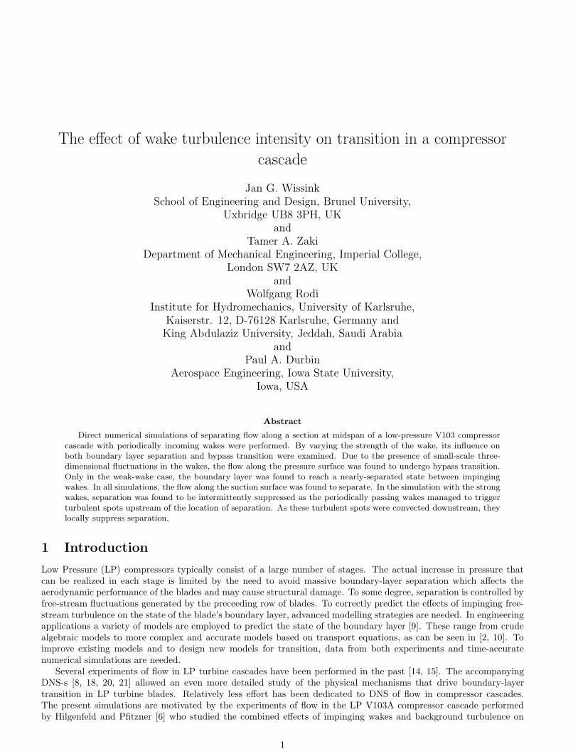
The phase-averaged turbulent kinetic energy 〈k〉 from simulation W2 is shown in figure 2 for 4 phases φ ={0, 2/8, 4/8, 6/8}. The increased levels of 〈k〉 identify the path of the incoming wakes as they migrate through thecompressor passage. In the inflow region, upstream of the leading edge of the blades, the upward moving wakesremain virtually straight. In the passage between blades, the wakes are slightly bent downwards by a moderatestretching/straining action of the mean flow. Because of this bending, the wakes impinge onto the suction side boundarylayer at non-zero angle of attack. Compared with the passing wakes in the T106 turbine cascade simulations [21]and [18], where production of turbulent kinetic energy was observed at the apex of the severely deformed wakes, in thecompressor passage - because of the significantly reduced turning and wake-distortion - no significant production of〈k〉 is observed. Only along the suction surface, immediately upstream of the trailing edge, an increased production ofkinetic energy is seen which is reflected by a local augmentation of 〈k〉 and indicates that the boundary layer underwenttransition to turbulence.

Figure 3 compares the phase-averaged turbulence levels 〈Tu〉 at mid pitch from simulations W1 and W2 at eightphases φ = {0, 1/8, 2/8, . . . , 7/8}. The local maxima in Tu identify the approximate location of the axis of the wakesas they are convected by the free-stream flow through the passage between blades. As expected, the convection speedof wakes in the two simulations is the same. The difference in intensity of the wakes in the passage between blades isa direct reflection of the difference in intensity at the inflow plane.

4

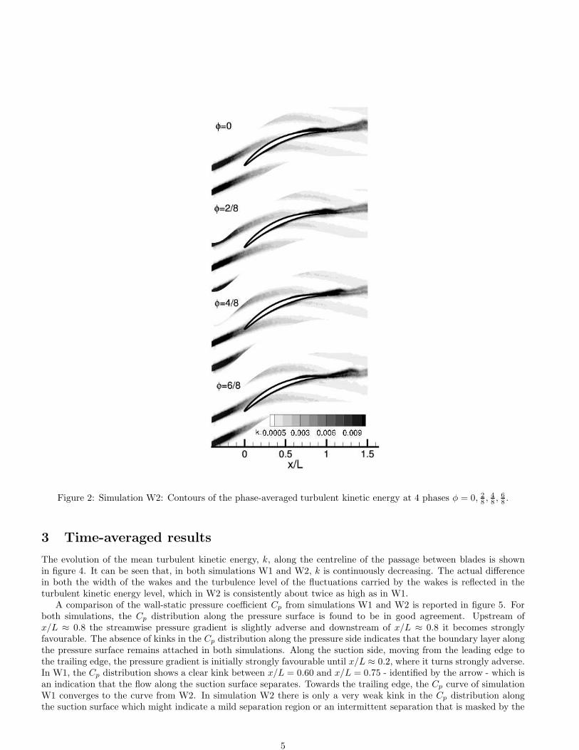
Figure 2: Simulation W2: Contours of the phase-averaged turbulent kinetic energy at 4 phases φ = 0, 2

8, 48, 6

8.

3 Time-averaged results

The evolution of the mean turbulent kinetic energy, k, along the centreline of the passage between blades is shownin figure 4. It can be seen that, in both simulations W1 and W2, k is continuously decreasing. The actual differencein both the width of the wakes and the turbulence level of the fluctuations carried by the wakes is reflected in theturbulent kinetic energy level, which in W2 is consistently about twice as high as in W1.

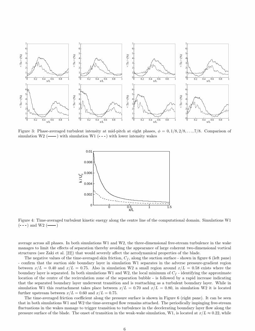
A comparison of the wall-static pressure coefficient Cp from simulations W1 and W2 is reported in figure 5. Forboth simulations, the Cp distribution along the pressure surface is found to be in good agreement. Upstream ofx/L ≈ 0.8 the streamwise pressure gradient is slightly adverse and downstream of x/L ≈ 0.8 it becomes stronglyfavourable. The absence of kinks in the Cp distribution along the pressure side indicates that the boundary layer alongthe pressure surface remains attached in both simulations. Along the suction side, moving from the leading edge tothe trailing edge, the pressure gradient is initially strongly favourable until x/L ≈ 0.2, where it turns strongly adverse.In W1, the Cp distribution shows a clear kink between x/L = 0.60 and x/L = 0.75 - identified by the arrow - which isan indication that the flow along the suction surface separates. Towards the trailing edge, the Cp curve of simulationW1 converges to the curve from W2. In simulation W2 there is only a very weak kink in the Cp distribution alongthe suction surface which might indicate a mild separation region or an intermittent separation that is masked by the

5

x/L

< T

u >

(%

)

0 0.2 0.4 0.6 0.8 10

1

2

3

4

5

6

7

x/L

< T

u >

(%

)

0 0.2 0.4 0.6 0.8 10

1

2

3

4

5

6

7

x/L

< T

u >

(%

)

0 0.2 0.4 0.6 0.8 10

1

2

3

4

5

6

7

x/L

< T

u >

(%

)

0 0.2 0.4 0.6 0.8 10

1

2

3

4

5

6

7

x/L

< T

u >

(%

)

0 0.2 0.4 0.6 0.8 10

1

2

3

4

5

6

7

x/L

< T

u >

(%

)

0 0.2 0.4 0.6 0.8 10

1

2

3

4

5

6

7

x/L

< T

u >

(%

)

0 0.2 0.4 0.6 0.8 10

1

2

3

4

5

6

7

x/L

< T

u >

(%

)

0 0.2 0.4 0.6 0.8 10

1

2

3

4

5

6

7

Figure 3: Phase-averaged turbulent intensity at mid-pitch at eight phases, φ = 0, 1/8, 2/8, . . . , 7/8. Comparison ofsimulation W2 ( ) with simulation W1 ( ) with lower intensity wakes

x/L

k/U

02

0 0.5 1 1.50

0.002

0.004

0.006

0.008

0.01

Figure 4: Time-averaged turbulent kinetic energy along the centre line of the computational domain. Simulations W1( ) and W2 ( )

average across all phases. In both simulations W1 and W2, the three-dimensional free-stream turbulence in the wakemanages to limit the effects of separation thereby avoiding the appearance of large coherent two-dimensional vorticalstructures (see Zaki et al. [22]) that would severely affect the aerodynamical properties of the blade.

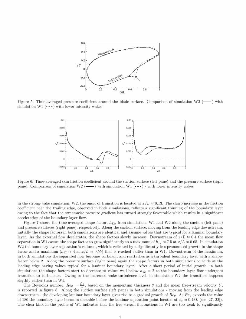
The negative values of the time-averaged skin friction, Cf , along the suction surface - shown in figure 6 (left pane)- confirm that the suction side boundary layer in simulation W1 separates in the adverse pressure-gradient regionbetween x/L = 0.40 and x/L = 0.75. Also in simulation W2 a small region around x/L = 0.58 exists where theboundary layer is separated. In both simulations W1 and W2, the local minimum of Cf - identifying the approximatelocation of the centre of the recirculation zone of the separation bubble - is followed by a rapid increase indicatingthat the separated boundary layer underwent transition and is reattaching as a turbulent boundary layer. While insimulation W1 this reattachment takes place between x/L = 0.70 and x/L = 0.80, in simulation W2 it is locatedfurther upstream between x/L = 0.60 and x/L = 0.75.

The time-averaged friction coefficient along the pressure surface is shown in Figure 6 (right pane). It can be seenthat in both simulations W1 and W2 the time-averaged flow remains attached. The periodically impinging free-streamfluctuations in the wakes manage to trigger transition to turbulence in the decelerating boundary layer flow along thepressure surface of the blade. The onset of transition in the weak-wake simulation, W1, is located at x/L ≈ 0.22, while

6

x/L

Cp

0 0.2 0.4 0.6 0.8 1-0.4

-0.2

0

0.2

0.4

0.6

Pressure side

Suction sideտ

Figure 5: Time-averaged pressure coefficient around the blade surface. Comparison of simulation W2 ( ) withsimulation W1 ( ) with lower intensity wakes

x/L

Cf

0 0.2 0.4 0.6 0.8 1-0.002

0

0.002

0.004

0.006

0.008

0.01

x/L

Cf

0 0.2 0.4 0.6 0.8 1-0.002

0

0.002

0.004

0.006

0.008

0.01

Figure 6: Time-averaged skin friction coefficient around the suction surface (left pane) and the pressure surface (rightpane). Comparison of simulation W2 ( ) with simulation W1 ( ) - with lower intensity wakes

in the strong-wake simulation, W2, the onset of transition is located at x/L ≈ 0.13. The sharp increase in the frictioncoefficient near the trailing edge, observed in both simulations, reflects a significant thinning of the boundary layerowing to the fact that the streamwise pressure gradient has turned strongly favourable which results in a significantacceleration of the boundary layer flow.

Figure 7 shows the time-averaged shape factor, h12, from simulations W1 and W2 along the suction (left pane)and pressure surfaces (right pane), respectively. Along the suction surface, moving from the leading edge downstream,initially the shape factors in both simulations are identical and assume values that are typical for a laminar boundarylayer. As the external flow decelerates, the shape factors slowly increase. Downstream of x/L ≈ 0.4 the mean flowseparation in W1 causes the shape factor to grow significantly to a maximum of h12 ≈ 7.5 at x/L ≈ 0.65. In simulationW2 the boundary layer separation is reduced, which is reflected by a significantly less pronounced growth in the shapefactor and a maximum (h12 ≈ 4 at x/L ≈ 0.55) that is reached earlier than in W1. Downstream of the maximum,in both simulations the separated flow becomes turbulent and reattaches as a turbulent boundary layer with a shape-factor below 2. Along the pressure surface (right pane) again the shape factors in both simulations coincide at theleading edge having values typical for a laminar boundary layer. After a short period of initial growth, in bothsimulations the shape factors start to decrease to values well below h12 = 2 as the boundary layer flow undergoestransition to turbulence. Owing to the increased wake-turbulence level, in simulation W2 the transition happenssligthly earlier than in W1.

The Reynolds number, Reθ = Uθν , based on the momentum thickness θ and the mean free-stream velocity U ,

is reported in figure 8. Along the suction surface (left pane) in both simulations - moving from the leading edgedownstream - the developing laminar boundary layer gives rise to a gradual growth of Reθ. As Reθ exceeds the valueof 180 the boundary layer becomes unstable before the laminar separation point located at xs ≈ 0.43L (see [27, 22]).The clear kink in the profile of W1 indicates that the free-stream fluctuations in W1 are too weak to significantly

7

x/L

h 12

0 0.2 0.4 0.6 0.8 10

2

4

6

8

x/L

h 12

0 0.2 0.4 0.6 0.8 10

1

2

3

4

Figure 7: Time-averaged shape factor along the suction surface (left pane) and the pressure surface (right pane).Simulations W1 ( ) and W2 ( )

x/L

Re θ

0 0.2 0.4 0.6 0.8 10

200

400

600

800

1000

x/L

Re θ

0 0.2 0.4 0.6 0.8 10

200

400

600

800

1000

Figure 8: Time-averaged Reθ along the suction surface (left pane) and the pressure surface (right pane). SimulationsW1 ( ) and W2 ( )

suppress separation, while the smoother behaviour of Reθ in W2 indicates that the free-stream fluctuations manageto significantly perturb the boundary layer thereby suppressing downstream separation. Further downstream in bothsimulations the boundary layer becomes fully turbulent and Reθ steadily grows until it reaches values aboveReθ = 1000near the trailing edge.

Along the pressure side (figure 8, right pane), immediately downstream of the leading edge the Reθ-values inboth simulations follow a similar trend. Once the boundary layer becomes unstable, however, in simulation W2 -withstronger disturbances - Reθ increases faster than in W1. This reflects the fact that the laminar-to-turbulent transitionin simulation W2 is established earlier than in W1. As can be seen from the Cf curve (figure Cf, right pane), transitionis completed at x/L ≈ 0.45 and 0.35 for W1 and W2, respectively. In both simulations, this corresponds to Reθ ≈ 350.

4 Phase-averaged and instantaneous results

4.1 The pressure surface

The transition mechanism on the pressure surface is examined in this section. The phase dependence of transition toturbulence and the change in the boundary layer between wakes are assessed. The transition mechanism is comparedto the canonical description of bypass transition, namely the formation of Klebanoff streaks in the boundary layerbeneath free-stream forcing, their secondary instability and the onset of turbulence spots [4, 23]. Finally, we examinewhether there is any evidence of the boundary layer relaxing to a nearly-separated state between impinging wakes.

8

x/L

Cf

0 0.2 0.4 0.6 0.8 10

0.001

0.002

0.003

0.004

0.005Simulation W1Simulation W2

φ = 0

x/L

Cf

0 0.2 0.4 0.6 0.8 10

0.001

0.002

0.003

0.004

0.005Simulation W1Simulation W2

φ = 1/4

x/L

Cf

0 0.2 0.4 0.6 0.8 10

0.001

0.002

0.003

0.004

0.005Simulation W1Simulation W2

φ = 2/4

x/LC

f0 0.2 0.4 0.6 0.8 10

0.001

0.002

0.003

0.004

0.005Simulation W1Simulation W2

φ = 3/4

Figure 9: Phase-averaged friction coefficient along the pressure side from Simulations W1 and W2. The actual locationof the wakes can be seen in Fig. 2

Figure 9 displays the phase-averaged skin friction, 〈Cf 〉, along the pressure surface of the blade from simulationsW1 and W2 at φ = {0, 1/4, 2/4, 3/4}. As the wakes migrate along the surface of the blade, disturbances are introducedinto the boundary layer. While in the absence of free-stream fluctuations the boundary layer on the pressure side wasfound to separate (see [27, 22]), in the presence of free-stream disturbances the boundary layer is likely to undergotransition to turbulence. The disturbances induced by the strong wakes (W2) are thereby expected to be more effectivein triggering transition to turbulence - corresponding to a significant growth in the friction coefficient - relative to theweak wakes (W1). This is evident in the 〈Cf 〉 curve at φ = 0, where the strong wakes of simulation W2 manage totrigger transition between x/L ≈ 0.13 and x/L ≈ 0.25. The slight kink observed in 〈Cf 〉 at x/L ≈ 0.38 corresponds toan earlier transition event triggered by the preceeding wake. With the weaker wakes from simulation W1, transitionoccurs further downstream and is located between x/L = 0.33 and x/L = 0.5. Also, it can be seen that the pressureside boundary layer from W1 does indeed relax to a nearly separated state near x/L = 0.35. A further reduction ofthe wake-passing frequency and/or the wake-turbulence is likely to induce periodic separation and separation-inducedtransition.

At φ = 1/4 the locations of transition in both simulations have moved with the wakes further downstream. Theonset of transition in W2 has moved to x/L ≈ 0.17. At the same location in W1, a slight increase in the phase-averagedskin friction can be observed. The distortion of the boundary layer, however, is not sufficient to cause a full transitionto turbulence, which happens further downstream and is still associated with the preceeding wake.

At φ = 2/4 transition in both simulations starts at x/L ≈ 0.25 and ends at x/L ≈ 0.35. The dips in the 〈Cf 〉signal near x/L ≈ 0.55 again correspond to an earlier transition event. The sequence of snapshots in figure 9 givea clear evidence of the presence of a periodic transition scenario in both simulations triggered by the passing wakes.In general the strong wakes in simulation W2 introduce stronger disturbances into the pressure side boundary layerwhich trigger earlier transition at φ = 0 and φ = 1/4.

Finally, at φ = 3/4 the onset of transition in both simulations has moved further downstream to x/L ≈ 0.27, whiletransition ends at x/L ≈ 0.40. In the simulation with strong wakes an incomplete transition event can be observedupstream, starting at x/L ≈ 0.10.

The contour plots in figure 10 (upper part) identify the location of the maximum phase-averaged spanwise fluctu-ations, maxy 〈wrms〉 (corresponding to the maximum value of 〈wrms〉 in the region between the wall and the edge ofthe boundary layer), in the pressure-surface boundary layer of simulations W1 (left) and W2 (right). The approximatepath of the wakes along the edge of the boundary layer is identified by the dashed lines and the calmed region thatforms in between impinging wakes is labelled “B”. The figure shows that there is a correlation between the presenceof the wake at the edge of the boundary layer and the presence of strong spanwise fluctuations inside the boundary

9

layer emerging after a slight phase-shift, ∆φ ≈ 0.3. The observed phase shift is explained partially by the fact thatthe location of the wake is given at the edge of the boundary layer while the location of maxy 〈wrms〉 is well inside theboundary layer - the time lag is necessary for free-stream disturbances to penetrate the boundary layer and to triggera response. Also, the propagation speed of disturbances inside the boundary layer is slower than that of the wake inthe free stream. This is evidenced by the existence of an angle between the path of the wakes and the orientationof the contours - best visible in simulation W1 - immediately downstream of the leading edge. The white areas inbetween the paths of the wakes, upstream of x/L ≈ 0.5, identify calmed regions in which the disturbance level insidethe boundary layer is relatively low. Further downstream disturbances are present inside the boundary layer at allphases indicating that at these locations the boundary layer is fully turbulent. Compared to the weak-wake simulationW1 (left pane), the contours of simulation W2 (right pane) show a smaller calmed region and an earlier transition toturbulence. Compared to maxy 〈wrms〉, the maximum tangential fluctuations, maxy 〈ut

rms〉, show a similar patternbut with slightly smaller calmed regions in between the paths of the migrating wakes. The main differences are thatthe maxima of the streamwise fluctuations are located more upstream than the maxima in the spanwise fluctuations,and that the actual level of the streamwise disturbances is significantly higher. A possible explanation for the ob-served differences is that the periodic disturbances introduced in the boundary layer by the passing wakes triggera Klebanoff distortion (streaks) which tends to lead to strong fluctuations in the streamwise direction and hence toa large maxy 〈ut

rms〉. Further downstream the streaks become unstable [17, 5] eventually leading to the observedamplification of maxy 〈wrms〉. The figure clearly demonstrates that both the appearence of streaks and the furthertransition to turbulence take place earlier in the strong wake simulation W2 relative to W1.

Figure 11 shows contours of the phase-averaged streamwise fluctuations along the pressure surface at phase φ = 7/8.The snapshot contrasts the location of maximum 〈ut

rms〉 within the pressure-surface boundary-layer to the locationalong the boundary-layer edge where the streamwise fluctuation level in the wake reaches its peak. This providesfurther evidence of the fact that the propagation speed of the wake-induced fluctuations inside the boundary layer isslower than the propagation speed of the wake in the free stream.

The four snapshots displayed in figure 12 show the time-evolution of contours of the tangential velocity fluctuationsin a plane adjacent to the pressure surface. The plane in the background - that shows contours of the fluctuatingvelocity - identifies the location of the wakes. As the wake traverses the surface of the blade, the boundary layer isperturbed. As a result, immediately below the wake, high- and low-speed streaks appear in the boundary layer. Atcertain times, a patch of calmed flow can be observed in between the passing wake and the turbulent flow downstream(see snapshots at t = 15.50 L/U and t = 15.75 L/U). The location of the onset of transition, associated with a passingwake, gradually moves downstream with the wake. Transition occurs when a number of turbulent spots appear almostsimultaneously at a similar streamwise location. These spots grow in the downstream direction and eventually mergeforming a fully-turbulent boundary layer.

Figure 13 shows contours of the spanwise velocity fluctuations and indicates where the streaks shown in figure 12become unstable resulting in the development of local patches of turbulence. A one-to-one comparison of the snapshotsin the two figures shows that the spanwise fluctuations first appear virtually at the same location as the first streaks.This evidences that when the wake triggers the formation of streaks in the pressure-surface boundary layer, it alsointroduces spanwise fluctuations. The latter contribute to streak instability and the onset of turbulence downstream.

4.2 The suction surface

Figure 14 shows a comparison of the phase-averaged friction coefficient, 〈Cf 〉, along the suction surface from simulationsW1 and W2. For all phases, the gradually decreasing 〈Cf 〉 profiles upstream of x/L = 0.4 are identical. It should benoted that in the absence of free-stream disturbances, the entirely laminar flow along the suction side separates alonga large portion of the blade [27, 22]. In that case the roll-up of the separated boundary layer resulted in the formationof strong two-dimensional KH rolls that convected downstream by the mean flow. In simulation W1, figure 14 showsthat the boundary layer separates at all phases, as indicated by 〈Cf 〉 becoming negative between x/L ≈ 0.45 andx/L ≈ 0.50. This is followed by a roll-up of the separated shear layer, which causes the significant oscillations in 〈Cf 〉downstream of x/L = 0.55.

Compared to simulation W1, the 〈Cf 〉 signal in simulation W2 is significantly smoother. At the phases shown, onlya small region of separation is identified as the separated boundary layer quickly undergoes transition to turbulenceand reattaches. Only around φ = 5/8 is separation of the time-averaged boundary layer entirely suppressed (seefigure 15). Even though this suppression is only marginal (the minimum 〈Cf 〉 value is virtually zero), it does showthat the increased wake-strength in simulation W2 not only leads to a significant reduction in the phase-averaged sizeof the separation bubble for all phases but also periodically leads to a complete reattachment of boundary layer.

10

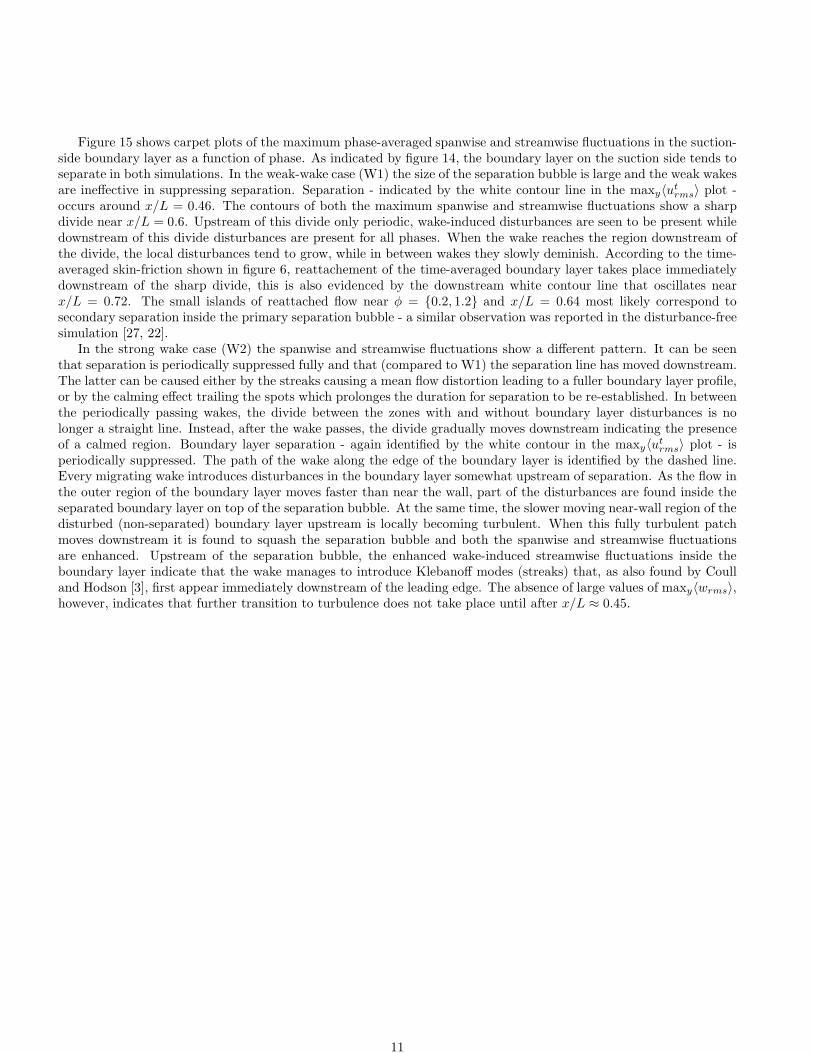
Figure 15 shows carpet plots of the maximum phase-averaged spanwise and streamwise fluctuations in the suction-side boundary layer as a function of phase. As indicated by figure 14, the boundary layer on the suction side tends toseparate in both simulations. In the weak-wake case (W1) the size of the separation bubble is large and the weak wakesare ineffective in suppressing separation. Separation - indicated by the white contour line in the maxy〈u

trms〉 plot -

occurs around x/L = 0.46. The contours of both the maximum spanwise and streamwise fluctuations show a sharpdivide near x/L = 0.6. Upstream of this divide only periodic, wake-induced disturbances are seen to be present whiledownstream of this divide disturbances are present for all phases. When the wake reaches the region downstream ofthe divide, the local disturbances tend to grow, while in between wakes they slowly deminish. According to the time-averaged skin-friction shown in figure 6, reattachement of the time-averaged boundary layer takes place immediatelydownstream of the sharp divide, this is also evidenced by the downstream white contour line that oscillates nearx/L = 0.72. The small islands of reattached flow near φ = {0.2, 1.2} and x/L = 0.64 most likely correspond tosecondary separation inside the primary separation bubble - a similar observation was reported in the disturbance-freesimulation [27, 22].

In the strong wake case (W2) the spanwise and streamwise fluctuations show a different pattern. It can be seenthat separation is periodically suppressed fully and that (compared to W1) the separation line has moved downstream.The latter can be caused either by the streaks causing a mean flow distortion leading to a fuller boundary layer profile,or by the calming effect trailing the spots which prolonges the duration for separation to be re-established. In betweenthe periodically passing wakes, the divide between the zones with and without boundary layer disturbances is nolonger a straight line. Instead, after the wake passes, the divide gradually moves downstream indicating the presenceof a calmed region. Boundary layer separation - again identified by the white contour in the maxy〈u

trms〉 plot - is

periodically suppressed. The path of the wake along the edge of the boundary layer is identified by the dashed line.Every migrating wake introduces disturbances in the boundary layer somewhat upstream of separation. As the flow inthe outer region of the boundary layer moves faster than near the wall, part of the disturbances are found inside theseparated boundary layer on top of the separation bubble. At the same time, the slower moving near-wall region of thedisturbed (non-separated) boundary layer upstream is locally becoming turbulent. When this fully turbulent patchmoves downstream it is found to squash the separation bubble and both the spanwise and streamwise fluctuationsare enhanced. Upstream of the separation bubble, the enhanced wake-induced streamwise fluctuations inside theboundary layer indicate that the wake manages to introduce Klebanoff modes (streaks) that, as also found by Coulland Hodson [3], first appear immediately downstream of the leading edge. The absence of large values of maxy〈wrms〉,however, indicates that further transition to turbulence does not take place until after x/L ≈ 0.45.

11

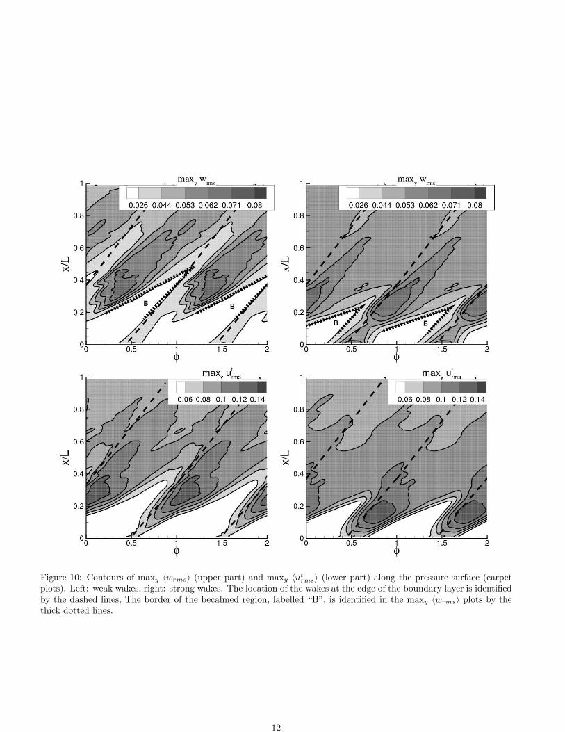
Figure 10: Contours of maxy 〈wrms〉 (upper part) and maxy 〈utrms〉 (lower part) along the pressure surface (carpet

plots). Left: weak wakes, right: strong wakes. The location of the wakes at the edge of the boundary layer is identifiedby the dashed lines, The border of the becalmed region, labelled “B”, is identified in the maxy 〈wrms〉 plots by thethick dotted lines.

12

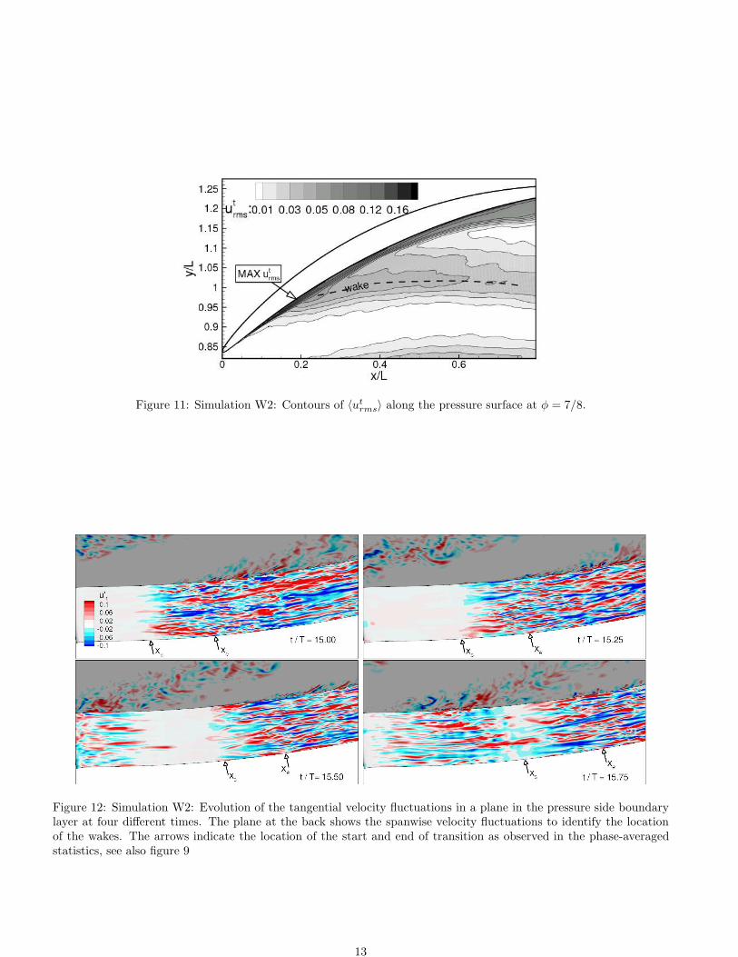
Figure 11: Simulation W2: Contours of 〈utrms〉 along the pressure surface at φ = 7/8.

Figure 12: Simulation W2: Evolution of the tangential velocity fluctuations in a plane in the pressure side boundarylayer at four different times. The plane at the back shows the spanwise velocity fluctuations to identify the locationof the wakes. The arrows indicate the location of the start and end of transition as observed in the phase-averagedstatistics, see also figure 9

13

Figure 13: Simulation W2: Evolution of the spanwise velocity fluctuations in a plane in the pressure side boundarylayer at four different times. The plane at the back shows the spanwise velocity fluctuations to identify the locationof the wakes. The arrows indicate the location of the start and end of transition as observed in the phase-averagedstatistics

x/L

<C

f>

0 0.2 0.4 0.6 0.8 1-0.01

-0.005

0

0.005

0.01

φ = 0

x/L

<C

f>

0 0.2 0.4 0.6 0.8 1-0.01

-0.005

0

0.005

0.01

φ = 1/4

x/L

<C

f>

0 0.2 0.4 0.6 0.8 1-0.01

-0.005

0

0.005

0.01

φ = 2/4

x/L

<C

f>

0 0.2 0.4 0.6 0.8 1-0.01

-0.005

0

0.005

0.01

φ = 3/4

Figure 14: Phase-averaged friction coefficient 〈Cf 〉 along the suction surface at phases φ = 0, 1/4, 2/4, 3/4. SimulationsW1 ( ) and W2 ( )

14

Figure 15: maxy〈utrms〉 and 〈wrms〉 along suction surface versus phase (carpet plot). Left: weak wakes (W1), right:

strong wakes (W2). The white contour in the maxy〈utrms〉 plots from simulations W1 & W2 identifies separation. As

in figure 10, the dashed lines correspond to the location of the wakes at the edge of the boundary layer.

15

φ

<C

f>

0 0.5 1 1.5 2-0.01

-0.005

0

0.005

0.01

x/L = 0.55

x/L = 0.60

x/L = 0.65

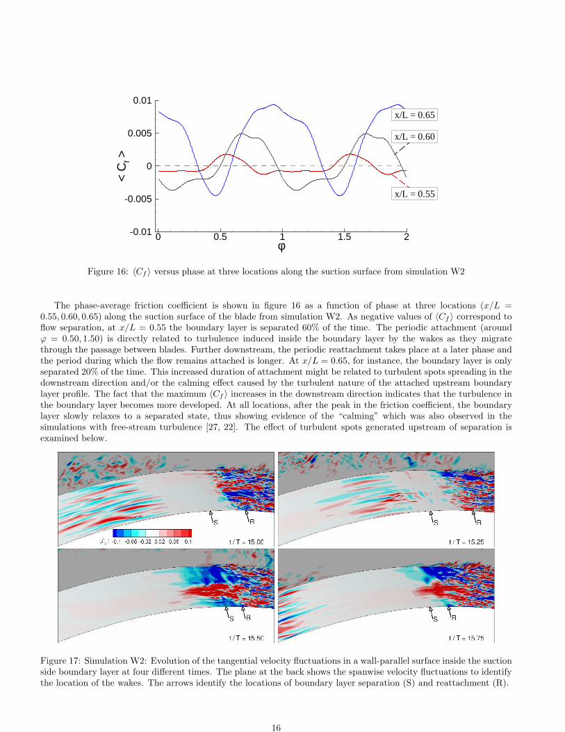
Figure 16: 〈Cf 〉 versus phase at three locations along the suction surface from simulation W2

The phase-average friction coefficient is shown in figure 16 as a function of phase at three locations (x/L =0.55, 0.60, 0.65) along the suction surface of the blade from simulation W2. As negative values of 〈Cf 〉 correspond toflow separation, at x/L = 0.55 the boundary layer is separated 60% of the time. The periodic attachment (aroundϕ = 0.50, 1.50) is directly related to turbulence induced inside the boundary layer by the wakes as they migratethrough the passage between blades. Further downstream, the periodic reattachment takes place at a later phase andthe period during which the flow remains attached is longer. At x/L = 0.65, for instance, the boundary layer is onlyseparated 20% of the time. This increased duration of attachment might be related to turbulent spots spreading in thedownstream direction and/or the calming effect caused by the turbulent nature of the attached upstream boundarylayer profile. The fact that the maximum 〈Cf 〉 increases in the downstream direction indicates that the turbulence inthe boundary layer becomes more developed. At all locations, after the peak in the friction coefficient, the boundarylayer slowly relaxes to a separated state, thus showing evidence of the “calming” which was also observed in thesimulations with free-stream turbulence [27, 22]. The effect of turbulent spots generated upstream of separation isexamined below.

Figure 17: Simulation W2: Evolution of the tangential velocity fluctuations in a wall-parallel surface inside the suctionside boundary layer at four different times. The plane at the back shows the spanwise velocity fluctuations to identifythe location of the wakes. The arrows identify the locations of boundary layer separation (S) and reattachment (R).

16

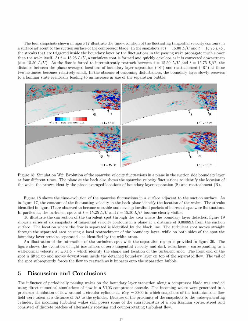
The four snapshots shown in figure 17 illustrate the time-evolution of the fluctuating tangential velocity contours ina surface adjacent to the suction surface of the compressor blade. In the snapshots at t = 15.00 L/U and t = 15.25 L/U ,the streaks that are triggered inside the boundary layer by the fluctuations in the passing wake propagate much slowerthan the wake itself. At t = 15.25 L/U , a turbulent spot is formed and quickly develops as it is convected downstream(t = 15.50 L/U). As the flow is forced to intermittently reattach between t = 15.50 L/U and t = 15.75 L/U , thedistance between the phase-averaged locations of boundary layer separation (“S”) and reattachment (“R”) at thesetwo instances becomes relatively small. In the absence of oncoming disturbances, the boundary layer slowly recoversto a laminar state eventually leading to an increase in size of the separation bubble.

Figure 18: Simulation W2: Evolution of the spanwise velocity fluctuations in a plane in the suction side boundary layerat four different times. The plane at the back also shows the spanwise velocity fluctuations to identify the location ofthe wake, the arrows identify the phase-averaged locations of boundary layer separation (S) and reattachment (R).

Figure 18 shows the time-evolution of the spanwise fluctuations in a surface adjacent to the suction surface. Asin figure 17, the contours of the fluctuating velocity in the back plane identify the location of the wakes. The streaksidentified in figure 17 are observed to become unstable and develop localised pockets of increased spanwise fluctuations.In particular, the turbulent spots at t = 15.25 L/U and t = 15.50 L/U become clearly visible.

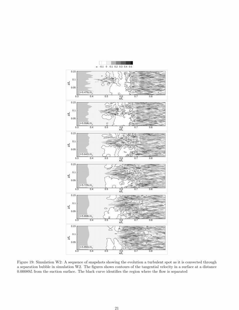
To illustrate the convection of the turbulent spot through the area where the boundary layer detaches, figure 19shows a series of six snapshots of tangential velocity contours in a plane at a distance of 0.00089L from the suctionsurface. The location where the flow is separated is identified by the black line. The turbulent spot moves straightthrough the separated area causing a local reattachment of the boundary layer, while on both sides of the spot theboundary layer remains separated - as identified by the white areas.

An illustration of the interaction of the turbulent spot with the separation region is provided in figure 20. Thefigure shows the evolution of light isosurfaces of zero tangential velocity and dark isosurfaces - corresponding to awall-normal velocity at ±0.1U - which identify the shape and location of the turbulent spot. The front end of thespot is lifted up and moves downstream inside the detached boundary layer on top of the separated flow. The tail ofthe spot subsequently forces the flow to reattach as it impacts onto the separation bubble.

5 Discussion and Conclusions

The influence of periodically passing wakes on the boundary layer transition along a compressor blade was studiedusing direct numerical simulations of flow in a V103 compressor cascade. The incoming wakes were generated in aprecursor simulation of flow around a circular cylinder at ReD = 3300 in which snapshots of the instantaneous flowfield were taken at a distance of 6D to the cylinder. Because of the proximity of the snapshots to the wake-generatingcylinder, the incoming turbulent wakes still posess some of the characteristics of a von Karman vortex street andconsisted of discrete patches of alternately rotating and counterrotating turbulent flow.

17

The effect of the strength of the wake on boundary-layer transition and boundary-layer separation was studied.On the pressure side, both the weak and strong wakes were found to trigger bypass transition of the boundary layerupstream of the location of separation identified in the disturbance-free simulation [27, 22]. As it passes over theblade, the strong wake induces transition shortly after the leading edge. The weaker wake causes transition furtherdownstream. However, when the wakes have passed mid-chord, the two cases have almost the same skin friction curveand in that sense, transition is independent of wake strength at that phase (see fig. 9). This is so, despite the weakwake having a lower turbulent intensity. This implies that correlations between transition and free-stream turbulentintensity are not applicable to transition under passing wakes: the instantaneous intensity is not correlated with theinstantaneous point of transition. The dynamics of the interaction between the wake and the boundary layer play adeterminative role.

At some phases, the wakes introduced disturbances into the boundary layer relatively close to the leading edge.These disturbances, however, were damped while convecting downstream, resulting in a re-laminarization of theboundary layer. This was seen on both pressure and suction sides of the blade. Despite the adverse pressure gradienton the pressure side, disturbances decay near the leading edge. This argues against leading edge receptivity beingthe initial coupling between the disturbance and the boundary layer. The passing wake provides evidence that thecoupling is locally to the downstream boundary layer. As they passed downstream, the boundary layer well upstreamof the wakes returned to laminar. In the weak-wake simulation, the boundary layer in between two passing wakes wasfound to relax to a nearly separated state. The strong-wake simulation relaxed too, but did not show any sign of beingclose to separation. Transition originates just behind the wakes and is caused by local forcing. This substantiates theidea that bypass transition is a consequence of low-frequency modes that penetrate into the boundary layer [24, 26].The consequent Klebanoff streaks are seen in the present simulations.

In the strong-wake-simulation it was found that separation on the suction surface was intermittently suppressed.In the weak-wake case the phase-averaged size of the suction-side separation bubble was only marginally affected bythe actual location of the wake. As a result, transition to turbulence was found to take place in the separated shearlayer and the location of transition was virtually independent of phase.

In the strong-wake simulation, the wakes introduced stronger disturbances in the suction side boundary layer,upstream of the location of separation. During each period, these disturbances were found to trigger streaks into theboundary layer which turned into turbulent spots as they were convected downstream. When reaching the locationof separation, the head of the turbulent spot - which was slightly lifted up - moved into the separated boundary layerwithout causing it to reattach (figures 19 and 20). This caused a prompt, 3-dimensional breakdown of the separatedshear layer. The flow underneath the spot was forced to locally reattach only when the tail of the spot reached theseparation bubble.

Future work on DNS of flows in turbomachinery could include - the effect of periodic unsteadiness in the overallpressure gradient on boundary layer transition (this unsteadiness would be created by the movement of blades upstreamof the passage), - simulation of more than one turbine/compressor passage, - simulation of a turbine/compressor passagewith end-wall effects etc.

Simulation results can be made available on request.

Acknowledgements

The authors would like to acknowledge the steering committee of the Computing Centre (HLRS) of the University ofStuttgart for granting computing time on the NEC SX8.

References

[1] Breuer, M., Rodi, W.: Large eddy simulation for complex flow of practical interest. In: E.H. Hirschel (ed.) Flowsimulation with high-performance computers II, Notes on Numerical Fluid Mechanics, volume 52. Vieweg Verlag,Braunschweig, Moscow: Nauka (1996)

[2] Cho, N.H., Liu, X., Rodi, W.: Calculation of wake-induced unsteady flow in a turbine cascade. ASME Paper92-GT-306 (1992)

[3] Coull, J., Hodson, H.: Unsteady boundary-layer transition in low-pressure turbines. J. Fluid Mech. 681, 370 –410 (2011)

18

[4] Durbin, P.A., Wu, X.: Transition beneath vortical disturbances. Annual Review of Fluid Mechanics 39, 107–128(2007)

[5] Hack, M.J.P., Zaki, T.A.: Streak instabilities in boundary layers beneath free-stream turbulence. Journal of FluidMechanics 741, 280–315 (2014)

[6] Hilgenfeld, L., Pfitzner, M.: Unsteady boundary layer development due to wake-passing effects on a highly loadedlinear compressor cascade. J. Turbomachinery 126, 493–500 (2004)

[7] Jacobs, R.G., Durbin, P.A.: Simulations of bypass transition. Journal of Fluid Mechanics 428, 185–212 (2001)

[8] Kalitzin, G., Wu, X., Durbin, P.: DNS of fully turbulent flow in a LPT passage. Int. J. of Heat and Fluid Flow24, 636–644 (2003)

[9] Mayle, R.E.: The role of laminar-turbulent transition in gas turbine engines. ASME Paper 91-GT-261 (1991)

[10] Michelassi, V., Martelli, F., Denos, T., Arts, T., Sieverding, C.: Unsteady heat transfer in stator-rotor interactionby two-equation turbulence model. ASME J. Turbomachinery 121, 436 – 447 (1999)

[11] Nagarajan, S., Lele, S., Ferziger, J.: Leading edge effects in bypass transition. Journal of Fluid Mechanics (2007)

[12] Nolan, K.P., Zaki, T.A.: Conditional sampling of transitional boundary layers in pressure gradients. Journal ofFluid Mechanics 728, 306–339 (2013)

[13] Rhie, C., Chow, W.: Numerical study of the turbulent flow past an airfoil with trailing edge separation. AIAA.J. 21(11), 1525–1532 (1983)

[14] Stadtmuller, P., Fottner, L.: A test case for the numerical investigation of wake-passing effects of a highly-loadedlp turbine cascade blade. ASME paper 2001-GT-311 (2001)

[15] Stieger, R., Hodson, H.: Convection of a turbulent bar wake through a low-pressure turbine cascade. ASME J.Turbomachinery 127, 388 – 394 (2005)

[16] Stone, H.: Iterative solutions of implicit approximations of multidimensional partial differential equations. SIAM.J. Nunerical Analysis 5, 87–113 (1968)

[17] Vaughan, N.J., Zaki, T.A.: Stability of zero-pressure-gradient boundary layer distorted by unsteady klebanoffstreaks. Journal of Fluid Mechanics 681, 116–153 (2011)

[18] Wissink, J.: DNS of separating low Reynolds number flow in a turbine cascade with incoming wakes. Int. J. ofHeat and Fluid Flow 24, 626–635 (2003)

[19] Wissink, J., Rodi, W.: Numerical study of the near wake of a circular cylinder. Int. J. of Heat and Fluid Flow29, 1060–1070 (2008)

[20] Wissink, J., Rodi, W., Hodson, H.: The influence of disturbances carried by periodically incoming wakes on theseparating flow around a turbine blade. Int. J. of Heat and Fluid Flow 27, 721–729 (2006)

[21] Wu, X., Durbin, P.A.: Existence of longitudinal vortices evolved from distorted wakes in a turbine passage.Journal of Fluid Mechanics 446, 199–228 (2001)

[22] Zaki, T., Wissink, J., Durbin, P., Rodi, W.: Direct numerical simulations of transition in a compressor cascade:the influence of free-stream turbulence. J. Fluid Mechanics 665, 57–98 (2010)

[23] Zaki, T.A.: From streaks to spots and on to turbulence: Exploring the dynamics of boundary layer transition.Flow, Turbulence and Combustion 91, 451–473 (2013)

[24] Zaki, T.A., Durbin, P.A.: Mode interaction and the bypass route to transition. Journal of Fluid Mechanics 531,85–111 (2005)

[25] Zaki, T.A., Durbin, P.A.: Continuous mode transition and the effects of pressure gradient. Journal of FluidMechanics 563, 357 – 388 (2006)

19

[26] Zaki, T.A., Saha, S.: On shear sheltering and the structure of vortical modes in single- and two-fluid boundarylayers. Journal of Fluid Mechanics 626, 111–147 (2009)

[27] Zaki, T.A., Wissink, J.G., Durbin, P.A., Rodi, W.: Direct computations of boundary layers distorted by migratingwakes in a linear compressor cascade. Flow, Turbulence and Combustion 83(3), 307–322 (2009)

20

u: -0.1 0 0.1 0.2 0.3 0.4 0.5

x/L

z/L

0.3 0.4 0.5 0.6 0.7 0.8

0.05

0.1

0.15

t=5.475L/U0

x/L

z/L

0.3 0.4 0.5 0.6 0.7 0.8

0.05

0.1

0.15

t=5.558L/U0

x/L

z/L

0.3 0.4 0.5 0.6 0.7 0.8

0.05

0.1

0.15

t=5.642L/U0

x/L

z/L

0.3 0.4 0.5 0.6 0.7 0.8

0.05

0.1

0.15

t=5.725L/U0

x/L

z/L

0.3 0.4 0.5 0.6 0.7 0.8

0.05

0.1

0.15

t=5.808L/U0

x/L

z/L

0.3 0.4 0.5 0.6 0.7 0.8

0.05

0.1

0.15

t=5.892L/U0

Figure 19: Simulation W2: A sequence of snapshots showing the evolution a turbulent spot as it is convected througha separation bubble in simulation W2. The figures shows contours of the tangential velocity in a surface at a distance0.00089L from the suction surface. The black curve identifies the region where the flow is separated

21

Figure 20: Simulation W2: A sequence of snapshots illustrating the movement of a turbulent spot (dark isosurfaces)through a separation bubble (light isosurface). The dark isosurfaces correspond to a wall-normal velocity of ±0.1Uand the light-gray isosurface corresponds to zero tangential velocity.

22