presented by presented by vinai ram, brandon ruben, rashaad aaron, stephan pierre, brandon maharaj,...

Presented by

Vinai Ram, Brandon Ruben, Rashaad Aaron, Stephan Pierre, Brandon Maharaj, Akim Mieres,

Makarion Phirangee

Class : 5P/5J

Teacher : Mr.G.PulchanSubject : Information Technology

What is a Spreadsheet?

• A spreadsheet is a table consisting of cells which enable a user to carry out numerical work easily. Spreadsheets also make use of formulae to manipulate this numerical data.

• Examples of a spreadsheet packages are• Microsoft Excel.• Apple iWork’s Numbers• Corel Quattro Pro (WordPerfect Office) )

What are the parts of a Spreadsheet?

A spreadsheet can be divided into the following parts:

• Rows• Columns• Cells

Rows………

• Rows are horizontal i.e. they run from left to right.

• Rows are numbered in ascending order.

Rows………

Columns…….

• Columns are vertical i.e. they run from top to bottom.

• Columns are lettered alphabetically.

Columns…….

Cells………

• A cell is the rectangular area where a row and a column meet.

• A cell is the intersection of a row and a column.

Cells……….

More on Cells…….

What was the definition of a cell?

…The intersection of a column and a row.• Columns are lettered…….• Rows are numbered……..

• The cell address is the location/position of the cell.

• It is written in terms of column letter then row number such as A17 B21 PL923.

Cell Address………

Name box showing active cell address i.e. the highlighted cell

Excel

• Each Excel document is called a workbook.

• A workbook can then be divided into individual worksheets.

Workbooks……Worksheets……

Title box showing name of workbook and program name

Menu bar showing worksheets

Functions….

Functions are predefined formulae in Excel that can automatically :

• Calculate results.• Perform worksheet actions.• Assist with decision making in the

spreadsheet.

Types of Functions….

There are many types of functions.• Sum function• Average• Date• Maximum and minimum• Count • If• Vlookup• Rank

SUM Function

• SUM is a predefined function in Excel. It is a quick and easy method to find the total of a group of cells.

• The Syntax for the SUM function is =SUM (number1, number2 …number255). Up to 255 numbers can be entered as arguments for the function.

• An argument is a value that is inserted into a function in order for it to carry out its task. It simply tells Excel what to do with the data in that location.

How to use the SUM function (shown by example).

• Click on cell D7 where results will be displayed.

• Click on the formulas tab of the ribbon menu.

• Choose Math & Trig from the ribbon to display dropdown menu.

• Click on sum from this menu to display function dialog box.

• The number1 line will already be selected, if not, select it.

• Click and hold cell D1 and drag down to D6 OR manually enter the first cell followed be a semicolon ( : ) and the last cell. (D1:D6)

• Click OK when finished and the answer (622) should be in cell D7.

More on the SUM function…….

• If numbers are input into the two spaces in the Excel document, the total will change as seen now…..

• This process can also be bypassed by selecting the formula menu then clicking the auto sum function, selecting the function you want and selecting the values to be processed…..

The Average function

• AVERAGE is a predefined function in Excel. It is a quick and easy method to find the mean of a group of cells.

How to use the AVERAGE function (shown by example).

• Click on cell D7 where the results will be displayed.

• Click on the formulas tab of the ribbon menu.

• Click on more functions to display the dropdown menu.

• Click on Statistical for another dropdown menu, here you can select AVERAGE.

• Drag select the cells you wish to calculate, in this case D1 to D6.

• A value will be automatically entered, click OK and you’re done.

More on the AVERAGE function…….

• If numbers are input into the two spaces in the Excel document, the mean will change as seen now…..


The DATE function……..

• The DATE function is a pre-defined Excel function. It is used simply to enter the date into a specific cell.

• It can be done by entering the syntax into the targeted cell. An example of this is:

• =DATE(2012, 9, 14).

Using the DATE function (shown by example)

• Click on a cell.• While that cell is targeted

select the formulas tab in the ribbon menu.

• Click on date & time to display the dropdown menu.

• The first thing on the drop down menu will be DATE.

• Select it and a window will pop up with spaces to enter year, month and day. Enter the values as directed and it will be formatted and entered into the specific cell.

The MAXIMUM function

• The Maximum function is one of Excel’s statistical functions. It is used to calculate the largest or maximum number in a given list of values or arguments.

• The syntax for Maximum function is =MAX (argument 1, argument 2 …argument30).

• These arguments can be numerical values, named ranges, arrays or cell references. Up to 30 cell references can be entered.

How to use the MAXIMUM function (shown by example)

• Click D7 and in the formulas tab of the ribbon menu, select More functions for the drop down menu.

• In the dropdown menu select Statistical then MAX, a window will appear.

• Using the cursor, select D1 and drag downwards until D1, D2, D3, D4, D5 and D6 is selected.

• Click the OK button in the pop-up window making sure the cells are highlighted.

• The largest number will be displayed in cell D7.

More on the MAXIMUM function…….

• If numbers are input into the two spaces in the Excel document, the maximum will change as seen now…..


The MINIMUM function

• The Minimum function is one of Excel’s statistical functions. It is used to calculate the lowest or minimum number in a given list of values or arguments.

• The syntax for the Minimum function is =MIN (argument 1, argument 2 …argument30).

• These arguments can be numerical values, named ranges, arrays or cell references. Up to 30 cell references can be entered.

How to use the MINIMUM function (shown by example)


• In the dropdown menu select Statistical then MIN, a window will appear.

• Using the cursor, select D1 and drag downwards until D1, D2, D3, D4, D5 AND D6 is selected.


• The lowest number will be displayed in cell D7.

More in the MINIMUM function

• If numbers are input into the two spaces in the Excel document, the minimum will change as seen now…..


The COUNT function

• The count function is a pre-defined system function in Excel that is used to total the number of cells in a selected range.

• The Count function only totals cells that contain numbers in them. The function ignores blank cells and cells with text data in them.

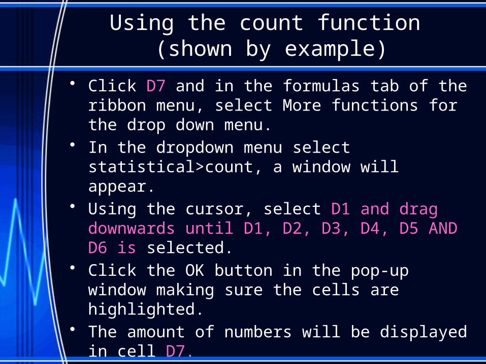
Using the count function (shown by example)


• In the dropdown menu select statistical>count, a window will appear.

• Using the cursor, select D1 and drag downwards until D1, D2, D3, D4, D5 AND D6 is selected.


• The amount of numbers will be displayed in cell D7.

The VLOOKUP function

• Excel's VLOOKUP function, which stands for vertical lookup, can help you find specific information in large data tables such as:

• An inventory list of parts • A large membership contact list

• Blank cells should be avoided as it renders the function inoperable.

How to use VLOOPKUP (shown by example)

• For this example the photo of preset values in Excel shown below will be used.

How to use VLOOPKUP (shown by example)

• Click on cell D1 and type the title Part Name.• Click on cell E1 and type the title Price.• Click on cell E2 - the location where the

results - in this case, the price of a Oil Filter - will be displayed.

• Click on the formulas tab in the ribbon menu and click on Lookup & Reference to open the dropdown menu

• In the drop down menu select VLOOKUP to display the dialog box.

The Dialog Box

• The data that we enter into the four blank rows of the dialog box will form the arguments for the VLOOKUP function.

• These arguments tell the function what information we are after and where it should search to find it.

The Lookup Value Argument(Area 1 in the Dialogue Box)

• The lookup value is located in the first column of the table of data. After specifying a subject in the first column, VLOOKUP will then allow you to search for specific information located in the same row as the subject.

• The lookup value can be text, a logical value (TRUE or

FALSE only), a number or a cell reference to a value.

• If you don’t use an absolute reference and you copy the VLOOKUP function to other cells, there is a good chance you will get error messages in the cells the function is copied to.

The Table Array Argument (Area 2 in the Dialog Box)

• The table array is the table of data that the VLOOKUP searches to find your information.

• The table array must contain at least two columns of data. The first column contains the lookup values (see previous step). These values can be text, numbers, or logical values.

• On this line in the dialog box enter the range of cells where the data is located.

• As with the lookup value, it is a good idea to use an absolute cell reference for the table array to avoid possible errors when copying the function.

The Table Array Argument (Area 2 in the Dialogue Box)

• Click on the Table_array line in the dialog box.

• Drag select cells D5 to E10 in the spreadsheet to add this range to the Table_array line. This is the range of data that VLOOKUP will search.

• Press the F4 key on the keyboard to make the range absolute.

Column Number Index Argument(Area 3 in the Dialog Box)

• The column index number indicates which column of the table array contains the data you are after.

For example:• If you enter a 2 into the column index number,

VLOOKUP returns a value from the second column of the Table_array;

• If the column index number is 4, it returns a value from the fourth column of the Table_array.

Column Number Index Argument(Area 3 in the Dialog Box)

• Click on the Col_index_num line in the dialogue box

• Type a 2 in this line to indicate that we want VLOOKUP to return information from the second column of the table array.

The Range Lookup Argument (Area 4 in the Dialog Box)

• The range lookup value is a logical value (TRUE or FALSE only) that indicates whether you want VLOOKUP to find an exact or an approximate match to the lookup value.

• If TRUE or if this argument is omitted, VLOOKUP will use an approximate match if it cannot find an exact match to the lookup_value. If an exact match is not found, VLOOKUP uses the next largest lookup value.

• If FALSE, VLOOKUP will only use an exact match to the lookup value. If there are two or more values in the first column of table_array that match the lookup value, the first value found is used. If an exact match is not found, an #N/A error is returned.

The Range Lookup Argument (Area 4 in the Dialogue Box)

• Click on the Range_lookup line in the dialog box

• Type the word False in this line to indicate that we want VLOOKUP to return an exact match for the data we are seeking.

• Click OK to close dialog box and complete the VLOOKUP function.

• If you have followed all the steps of this tutorial you will have a complete VLOOKUP function in cell E2.

The RANK function

• The rank function is one of Excel’s pre-defined system functions.

• It is a statistical function and it ranks the size of a number compared to other numbers in a list a data.

The RANK function

• The syntax for the RANK function is:

= RANK ( Number, Ref, Order )• Number - the cell reference of the number to be

ranked.• Ref - the range of cells to use in ranking the Number.

• Order - determines whether the Number is ranked in ascending or descending order.

• Type a "0" (zero) to rank in descending order (largest to smallest). Type a 1 to rank in ascending order (smallest to largest).

Using the RANK function

• Click on the Formulas tab.• Choose More Functions > Statistical from the ribbon to open the

function drop down list.• Click on RANK in the list to bring up the function's dialog box. • Click on cell F4 to choose the number to be ranked (345). • Click on the "Ref" line in the dialog box. • Drag select cells D1 to D11 in the spreadsheet to enter the range into

the dialog box.• Click on the "Order" line in the dialog box. • Type a zero on this line to rank the number in descending order. • Click OK. • The number 1 should appear in cell F4 since the number 345 is the

largest number. • The complete function = RANK ( D4 ,D1:D11,0) appears in the formula

bar above the worksheet when you click on cell F4.

The IF function

• The IF function test to see whether a certain condition is true or false.

• The syntax for the IF function is:• =IF( logical_test, value_if_true, value_if_false )• logical_test - a value or expression that is tested to

see if it is true or false.• value_if_true - the value that is displayed if

logical_test is true.• value_if_false - the value that is displayed if

logical_test is false.

Using the IF function (shown by example)

• Click on the Formulas tab.• Choose Logical Functions from the ribbon to open the drop

down list.• Click on IF in the list to bring up the function's dialog box. • On the Logical_test line in the dialog box, click on cell D1. After

this type the less than symbol ( < ) and then the number 26. • On the Value_if_true line of the dialog box, type 100.• On the Value_if_false line of the dialog box, type 200.• Click OK • The value 200 should appear in cell E1, since the value in D1 is

greater than 26.

The Nested IF function

• The nested If function is used when many conditions need to be tested.

• The following example would demonstrate this……….

Formulae Usage in Excel

Some important points to remember about Excel formulas:

• Formulas in Excel always begin with the equal sign ( = ).

• The equal sign always goes in the cell where you want the answer to go.

• Use of brackets is very helpful.

Use Cell References in Formulas

• Even though you can use numbers directly in a formula, it is much better to use the references or addresses of the cells containing the numbers you want to use.

• If you use the cell references rather than the actual data, later, if you need to change the data or copy it in either cell, the results of the formula will update automatically without you having to rewrite the formula.

Addition Subtraction Multiplication Division

• Using what we have just learnt is quite easy :

• Addition =(A1+B1)• Subtraction=(A1-B1)• Multiplication =(A1*B1)• Division =(A1/B1)

• This would be the basic format for any formula you may wish to form…

Remember

Equal Sign

ParenthesisArithmetic Sign

Cell Address

Formulas with Exponents

• In Excel powers are represented by ^ followed by the cell reference.

• Cell references are preferred as if the values of the cells are to be changed the result will also change.

Format for Exponential Equations

• As with all other formulas the basic format still applies here.

• This format is : =(Cell address ^ Cell address)

e.g. =(E1^F1)

Formulas with Square Roots

• In Excel square roots are represented by SQRT followed by cell reference.

• Cell references are preferred as if the values of the cells are to be changed the result will also change.

Format for Formulas With Square Root

• The syntax for the SQRT function is:

= SQRT ( Number )

• This SQRT function can also be accessed by clicking the Formula tab>Math & Trig>SQRT and then filling in the cell address in the Number space in the dialog box.

Formulas with Brackets

• If more than one operator is used in a formula, there is a specific order that Excel will follow to perform these mathematical operations.

• This order of operations can be changed by adding brackets to the equation. An easy way to remember the order of operations is to use the acronym:

• BEDMAS

BEDMAS

The Order of Operations is:• Brackets• Exponents• Division• Multiplication• Addition• Subtraction

• Basically whatever is put into brackets will be calculated firstly.

Row/column Title Locking

• When you freeze panes, you select specific rows or columns that remain visible and present when scrolling throughout the worksheet.

• This is especially helpful when there are standard headings used for rows and columns within a worksheet.

How to Lock Specific Rows or Columns

• To lock rows, select the row below the row or rows that you want to keep visible when you scroll.

• To lock columns, select the column to the right of the column or columns that you want to keep visible when you scroll.

• To lock both rows and columns, click the cell below and to the right of the rows and columns that you want to keep visible when you scroll.

How to Lock Specific Rows or Columns

• On the View tab, in the Window group, click the arrow below Freeze Panes.

• Do one of the following:– To lock one row only, click Freeze Top Row.– To lock one column only, click Freeze First

Column.– To lock more than one row or column, or to lock

both rows and columns at the same time, click Freeze Panes.

The Address Function

You can use the ADDRESS function to obtain the address of a cell in a worksheet, given specified row and column numbers.

For example:• ADDRESS(2,3) returns $C$2.• ADDRESS(77,300) returns $KN$77.

You can use other functions, such as:• the ROW and COLUMN functions, to provide the row and

column number arguments for the ADDRESS function.

Syntax• ADDRESS(row_num, column_num, [abs_num], [a1],

[sheet_text])


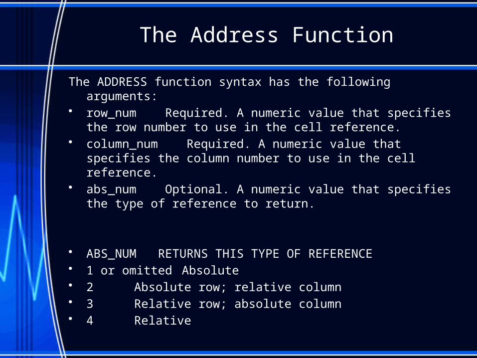
The ADDRESS function syntax has the following arguments:• row_num Required. A numeric value that specifies the row number to

use in the cell reference.• column_num Required. A numeric value that specifies the column

number to use in the cell reference.• abs_num Optional. A numeric value that specifies the type of

reference to return.

• ABS_NUM RETURNS THIS TYPE OF REFERENCE• 1 or omitted Absolute• 2 Absolute row; relative column• 3 Relative row; absolute column• 4 Relative


A1 is Optional.

It is a logical value that specifies the A1 or R1C1 reference style.

• A1 style - columns are labelled alphabetically rows are labelled numerically.

• R1C1 reference style, both columns and rows are labelled numerically.

• If the A1 argument is TRUE or omitted, the ADDRESS function returns an A1-style reference; if FALSE, the ADDRESS function returns an R1C1-style reference.

• NOTE To change the reference style that Excel uses, click the Microsoft Office Button ,click Excel Options, and then click Formulas. Under Working with formulas, select or clear the R1C1 reference style check box.


• Sheet_text is Optional.

• A text value that specifies the name of the worksheet to be used as the external reference.

Example formula =ADDRESS(1,1,,,"Sheet2") returns

Sheet2!$A$1.

• If the sheet_text argument is omitted, no sheet name is used, and the address returned by the function refers to a cell on the current sheet.

Replicating (copying) Formulae into other Cells

• Relative cell addressing with formulae is default set type of cell addressing.

• It means that as formula is replicated to other cells the cell address in the formula is automatically changed to suit the new location.

• Problems however, may arise if a cell in the formula is in one cell alone yet this cell data is needed by other cells to carry out a function. Here absolute cell addressing may be used.

Replicating (copying) Formulae into other Cells

• There may be instances where the user does not want Excel to change the cell address.

• To prevent alteration of these references a dollar ($) sign can be placed before and after the column number. Pressing the F4 key on the keyboard makes the reference absolute.

• These values will now undergo no change when copied or moved anywhere across spreadsheet.

Manipulating Data on the SpreadsheetCopying

• There are several situations which could arise if a formula is copied depending on the type of cell addressing used.

• Relative Cell Addressing • The destination cell will only contain the same data if the cells

used in the formula contain the same data as the cells used in the original formula. If not the data output in the formula destination cell will be calculated using data from the relative cells.

• Absolute Cell Addressing• The destination cell will contain the same data provided all cells

used in the formula use absolute cell addressing. Otherwise the situation would be the same as stated above for the cells not using absolute cell addressing.

Manipulating Data on the SpreadsheetCopying

To copy formulae simply: • Right-click the cell using the formula. • Select copy from the drop-down list. • Afterwards simply select the desired cell • Right-click it and select paste from the drop-

down list.

Manipulating Data on the Spreadsheet Moving Formulae

• If a formula is moved from one cell to another, the destination cell will contain the same data. The type of cell addressing which the cells used in the formula had would not affect the data.

• If the cell the formula was moved from was used in another calculation, the output of this calculation would be altered or an error message displayed.

Manipulating Data on the Spreadsheet Moving Formulae

To move formulae around the spreadsheet simply:

• Right-click the cell using the formulae .• Select cut from the drop-down list.• Next simply right-click the desired cell for

destination of formulae.• Select paste from the drop-down list.

Manipulating Data on the SpreadsheetDeleting Formulae

• If formulae is deleted there would be no calculation done and hence the data from the calculation would be deleted as well.

• If the data from this cell had been linked to other cells they too would be altered or deleted.

• To delete formulae simply right-click the desired cell and select clear contents from the drop-down list.

Manipulating Data on the Spreadsheet Columns and Rows

• New rows and columns can be inserted into a spreadsheet.

• This would create a new blank column or row in the spreadsheet adjusting the location of cells.

• These new columns or rows will not affect any previous information on the spreadsheet

• The new column would the inserted to the left of the column selected.

• The row will be inserted above the row selected.


To insert a column simply:• Right-click the column header of the column

which is desired to be on the right of the new column and select insert from the drop-down list.

To inserted a row simply :• Right-click the row header of the column

which is desired to be at the bottom of the new row and select insert from the drop-down list.


• Similarly rows and columns can be deleted.

• All data in the cells in these rows or columns will be removed.

• If any data in these now-deleted cells were previously being used for a calculation by another cell an error message would be produced in that cell.


To delete a column simply:• Right-click the column header of the column

which is desired to be deleted and select delete from the drop-down list.

To delete a row simply • Right-click the row header of the row which is

desired to be delete and select delete from the drop-down list.

Formatting a Spreadsheet Numeric Data Formatting

• Formatting numeric data refers to changing or altering the way in which numbers are represented.

Some standard formats are:• General – no specific number format• Number – general display of numbers (that is

decimal places and negative numbers)

• Currency – for monetary values (an example, $2971.83) {Specialized

Formatting Option} • Accounting – for lining up currency symbols and

decimal points {Specialized Formatting Option}

Formatting a Spreadsheet Numeric Data Formatting

To format the numeric data in a worksheet:• Highlight the cell or range of cells to be formatted.• Click the “Format” option listed under the “Home” section.• Click the “Format Cells” option listed under “Format”. When a

new window opens, click the “Number” option listed at the top, if it is not already selected.

• Select from the list, “Category”, whichever option is best suited to obtain the desired format of the data.

• Once the desired choice is highlighted, click “OK” to apply the changes to the document.

OR• You can select an option from a drop-down list or otherwise,

which is shown in the subsection “Number”, listed in the section “Home”.

Formatting a Spreadsheet

• Formatting data allows the user to alter and determine the outcome and appearance of the document.

• It allows the user to control what is produced.

Formatting a Spreadsheet Text Formatting

• Formatting the text within a worksheet document refers to changing or altering the way in which the text data is displayed.

Formatting a Spreadsheet Text Formatting

• Highlight the cell or range of cells, which contain text data, to be formatted.

• Click the “Format” option listed under the “Home” section.• Click the “Format Cells” option listed under “Format”.• A new window is opened, where the user is able to format

aspects of the text, such as font, font style, size and colour.• Select the desired options, then click “OK” when finished.

OR• You can select an option from a drop-down list or otherwise,

which is shown in the subsection “Font”, listed in the section “Home”.

Formatting a SpreadsheetText Alignment

• This function allows the user to change or move the position of text within a cell or range of cells.

• The user is allowed to change aspects such as, the degree of the indent of the text, its direction, as well as its orientation.

Formatting a SpreadsheetText Alignment

• Highlight the cell or range of cells to be formatted.• Click the “Format” option listed under the “Home”

section.• Click the “Format Cells” option listed under “Format”.• When a new window is opened, click the “Alignment”

option listed at the top.• Select the desired options from the drop-down lists

and from those that are listed, then click “OK” when finished, to apply the changes to the text in the document.

Formatting a SpreadsheetBorders

• This function allows the user to …

• Apply or remove borders from the worksheet.• Select where the border is to be placed • Change its style and colour.

Formatting a SpreadsheetBorders

• Highlight the cell or range of cells to which the border is to be applied.

• Click the “Format” option listed under the “Home” section.

• Click the “Format Cells” option listed under “Format”.• When a new window is opened, click the “Border”

option listed at the top.• Select the style and colour of the border, as well as,

choose where the border is to be applied from the options that are listed.

• Click “OK” when finished, to apply the changes to the document.

Sorting a Spreadsheet

• Sorting data in a spreadsheet refers to arranging it in some order.

• A typical spreadsheet package enables the user to sort data, whether text or numbers, into either ascending or descending order.

• In Excel, if an order is not specified, the rows and columns are sorted in ascending order, that is, the lowest to the highest.

Sorting a Spreadsheet

• When sorting a spreadsheet, there are primary fields and secondary fields.

• A primary field or primary column is the column that will be sorted first, when a command is given.

• A secondary field or secondary column is the column that is sorted after the primary column has already been sorted.

Sorting in Ascending and Descending Order

• Select the cell in the column that you wish to sort.• Click the “Data” option listed at the top of the window.• Click the option “Sort” from the section titled “Sort &

Filter”.• When a new window opens, select the order from the

drop-down list, either “A to Z” (ascending) or “Z to A” (descending).

OR• Select the desired cell then click the option “Data”

listed at the top of the window. • From the section listed “Sort & Filter” choose the

options listed, whether “A to Z” or “Z to A”.

Sorting using Primary and Secondary Fields

• Select the cell in the column that you wish to sort.• Click the “Data” option listed at the top of the window.• Click the option “Sort” from the section titled “Sort &

Filter”.• When a new window opens, use the “Sort by” box to

select the primary column by which you want your data sorted.

• To add a secondary field, click the “Add Level” option listed at the top of the “Sort” window.

• Use the “Then by” box to select the secondary column by which you want to sort your data.

• Click the “OK” option to apply the changes to the document.

Finding a Record Matching Given a Criterion

• Filtering a worksheet displays records that contain a certain value or that meet a set of criteria. There are two (2) methods used for filtering records in Excel. They are “Filter” and “Advanced Filter”.

Filter and Advanced Filter

• The option “Filter” allows the selection of records based on one criterion.

• The option “Advanced Filter” allows the use of multiple or complex criteria to limit which records are included in the result set of a query.

Filter and Advanced Filter

N.B. Before a worksheet can be filtered it must have column labels.

• LIST RANGE - this is the range of cells that you will perform the advanced filter function on.

• CRITERIA RANGE - this is the range of cells that contain the various criteria which will be used to select the records and generate the query result.

• COPY LOCATION - this is the area in the worksheet or where the query result will be

displayed.

Filter Command

• Click any cell that contains data. • Click the option “Data” listed at the top of the window.• Click the option “Filter” listed in the section “Sort &

Filter” OR press [Ctrl+Shift+L].• Once filtering is turned on, click the arrow in the

column header to choose a filter for the column from the drop-down list shown.

• Click “OK” to apply the changes to the document.

Advanced Filter Command

• Copy all headings and paste them in another location on the document.

• Add the criteria under the appropriate labels, that will be used to search the main document and generate the query result.

• Click the option “Data” listed at the top of the window.• Click the option “Advanced” listed in the section “Sort

& Filter”.• When the “Advanced Filter” window opens, specify

the list range, criteria range and copy location (if necessary).

• Click “OK” to display the query result.

Charts in Excel

• Charts are basically graphical representations of data.

• They are intended to make data easier to read, understand and interpret.

• There are several chart types and consequently many ways of displaying the same information.

Creating Charts on Excel

• Input data in Excel spreadsheet

• Highlight data to be represented in chart

• Select tab “Insert”

• From menu that has appeared, select one of the following chart types:– Column– Line– Pie– Bar– Area– Scatter

• Click on your choice of chart type and select one from the options that appear.

Adding a Chart Title

• Click anywhere on the chart

• From the menu options select “Layout” tab under chart tools

• From the menu list click on “Chart Title” then select the positioning of your title

• A text will then appear. Click on it and then enter the title of your chart

Adding Axis Titles

• Click anywhere in the chart• The display “Chart Tools” appears and the Tabs, Design, Layout

and Format become available. Click on the Layout tab.• Under the Layout tab, select Axis titles.• Do one or more of the following:

– To add a title to the horizontal axis, click on the “Primary Horizontal Axis Title” and then click the option that you want.

– To add a title to the vertical axis, click on “Primary Vertical Axis Title”, and then click the option that you want.

– To add a title to a depth axis, click “Depth Axis Title” and then click the option you want.

– In the text box that appears, type the title you want.

Data Manipulation in Multiple Worksheets

• Multiple worksheets are used to separate data into categories. Manipulating data in multiple worksheets is a necessary skill for solving complex problems. A user may wonder :

• Is it possible to enter the same data into several worksheets without retyping or copying and pasting the text into each one?

• How can you easily sum the cell values across multiple worksheets?

• How can you list the names of the worksheets in your workbook?

Entering Data in Multiple Worksheets Simultaneously

• As an example, let's say you want to put the same title text into different worksheets.

• One way to do this is to type the text in one worksheet, and then copy and paste the text into the other worksheets.

• If you have several worksheets, this can be very tedious……………..

Entering Data in Multiple Worksheets Simultaneously

• Press and hold the CTRL key, and then click Sheet1, Sheet2, and Sheet3.

• Click in cell A1 in Sheet1, and then type: **********

(This data will appear in each sheet).

• Click Sheet2 and notice that the text you just typed in Sheet1 also appears in cell A1 of Sheet2. The text also appears in Sheet3.

Sum the Value of a cell across Multiple Worksheets

• Another common Excel task is to sum the value of a cell in multiple worksheets and then display the result in another cell.

Sum the Value of a cell across Multiple Worksheets

• In cell B8 in Sheet1, type 20.• In cell B8 in both Sheet2 and Sheet3,

type 30.• In cell B9 in Sheet1, type the following

formula:=SUM(Sheet1:Sheet3!B8)

• Press ENTER. Notice that cell A1 displays 80, which is the total sum of the cells in the three worksheets.

Consolidate Data In Multiple Worksheets

• To summarize and report results from separate worksheets, you can consolidate data from each worksheet into a master worksheet.

• The worksheets can be in the same workbook as the master worksheet or in other workbooks.

• When you consolidate data, you are assembling data so that you can easily update and merge it on a regular or ad hoc basis.


• To consolidate data, use the Consolidate command in the Data Tools group on the Data tab.

• Consolidate by formula

• On the master worksheet, copy or enter the column or row labels that you want for the consolidated data.

• Click a cell that you want to contain consolidated data.

• Type a formula that includes a cell reference to the source cells on each worksheet or a 3-D reference that contains data that you want to consolidate. Regarding cell references, do one of the following:


• If the data to consolidate is in different cells on different worksheets

• Enter a formula with cell references to the other worksheets, one for each separate worksheet. For example, to consolidate data from worksheets named Advertising (in cell C8), Utilities (in cell G6) and Rent (in cell T6) of the master worksheet, you would enter the following:

• Tip :To enter a cell reference, such as Utilities!G6, in a formula without typing, type the formula up to the point where you need the reference, click the worksheet tab, and then click the cell.


• If the data to consolidate is in the same cells on different worksheets

• Enter a formula with a 3-D reference that uses a reference to a range of worksheet names. For example, to consolidate data in cells A3 from Advertising through Rent inclusive, in cell A3 of the master worksheet you would enter the following:

• NOTE If the workbook is set to automatically calculate formulas, a consolidation by formula always updates automatically when the data in the separate worksheets change.

Importing Graphics into Excel

• You can insert many popular graphics file formats into your workbook either directly or with the use of separate graphics filters. You don't need a separate graphics filter installed to insert the following graphics file formats:

• Enhanced Metafile (.emf)• Joint Photographic Experts Group (.jpg)• Portable Network Graphics (.png)• Microsoft Windows Bitmap (.bmp, .rle, .dib)• Graphics Interchange Format (.gif)• Windows Metafile (.wmf) graphics

Importing Graphics into Excel

• On the Insert tab, click the Picture button in the Illustrations group.

• The Insert Picture dialog box appears.• Locate and select the picture file you want to

import.• Click the Insert button.• The selected picture appears in the

worksheet.• Move and resize the image as needed.

Importing Tables into Excel

• If the data table is in a Word document or in text format on a webpage, change its format by saving the file/page as a text file. To do that:– Click on the File menu, top left corner of window, select Save

As– Accept the default file name or change it, but be sure to

select File Type– Text File (.txt) from the options available in the scroll menu. Remember where you save this file.

• On Excel, click on File>Open and select the document.• A Text Import Wizard box will open prompting you to select how

you want the data to appear when viewed using Excel. Work through the options presented – in some cases the Wizard will preview what an option will look like in the final imported file.

More on Importing Tables into Excel

• You may need to do some editing if you wish to work efficiently with the imported data.

• If a small green triangle appears in the upper left hand corner of any spreadsheet cells, that is an indicator that you have options to choose from. The data in the cell has been given a default format (text, numeric, etc) which you may want to change.

• For example, if numbers are stored in cells as text you will not be able to perform mathematical calculations using Excel formulas. Click in any cell with numbers in it, right click and select CELL FORMAT from the pull down menu that appears. Select from among the several number categories that which best defines the nature of the data.

A Presentation by:

Vinai Ram (Group Leader)

Brandon Ruben

Rashaad Aaron

Brandon Maharaj

Akim Mieres

Makarion Phirangee

5P/5J IT CLASS PCC

Thank You

presented by presented by vinai ram, brandon ruben, rashaad aaron, stephan pierre, brandon maharaj,...

Documents

highlighted cell slide

sum function sum

cell d1

cell d7

auto sum function

vlookup rank slide

information technology

predefined function