presentation european actuarial journal conference 2016

A discount curve for Insurance Risk Managementwith exact fit and parsimonious forecasts

Thierry Moudiki, PhD candidate @ ISFA Laboratoire SAF (jointwork with Areski Cousin & Ibrahima Niang)

08 septembre 2016

Plan

1. Context2. Curve construction and extrapolation

I Curve constructionI Curve extrapolation

3. Real world forecasting

1. Context




1. Context

I Calculation of insurers’ technical provisionsI Discount curve calibration and extrapolation for pricing and

risk neutral simulationI Curves’ real world forecasting for risk management

2. Curve construction and extrapolation

2.1. Curve construction





2.1. Curve construction

I Discount curve construction: uses IRS + Credit RiskAdjustment (Solvency II framework) or OIS

I Curve construction methodology: ideas from Schlögl andSchlögl (2000)

I We add:I static discount curve extrapolationI curves’ real world forecasting

I Can be extended to multiple curve construction


2.1. Curve construction (cont’d)

I Idea: No arbitrage short rate models include t 7→ b(t) forexact fitting of initial term structure

I Examples:I Hull & White (1990, 1994) extended VasicekI Extended CIR. . .

I piecewise-constant specification of t 7→ b(t) at inputswaps’ maturities T1, . . . ,Tn −→ b1, . . . , bn

2. Curve construction and extrapolation2.1. Curve construction (cont’d)

I Discount factors in the extended Vasicek case:

P(0, t) = exp(−X0φ(t)− a

∫ t

t0b(u)φ(t − u)du − ψ(t)

)Where:

φ(s) := 1a(1− e−as)

ψ(s) := −∫ s

0

(σ2

2 φ2(s − θ)

)dθ

I Piecewise-constant t 7→ b(t):∫ t

0b(u)φ(t − u)du −→

n∑k=1

bk

∫ Tk∧t

Tk−1∧tφ(t − u)du −→ PM(0, t)


2.1. Curve construction (cont’d)

I Calibration?I S = swaps values at time t = 0I C = swaps cash flows matrixI W = diagonal matrix of minimization weightsI P = unknown discount factors, function of b1, . . . , bn

I From less bias (and more variance) to more bias (and lessvariance)

I Solve S = CP iteratively (a.k.a bootstrapping)I Minimize (S − CP)T W (S − CP)I Minimize (S − CP)T W (S − CP) + Penalization


2.2. Curve extrapolation




2. Curve construction and extrapolation2.2. Curve extrapolation

I In the Extended Vasicek case, for t > Tn add a parameter:

bn+1 = f∞ + σ2

2a2

where f∞ = UFR = Ultimate Forward RateI Either exogenously fixed UFR and convergence periodτconvergence : increase parameter a until

|f M(0, LLP + τconvergence)− f∞| < tolerance

I Or data driven UFR:I A fraction of the swaps data in a training set, the other in atest set

I A grid search on values for f∞ −→ lowest pricing error on swapsfrom the test set

2. Curve construction and extrapolationI IRS from Ametrano and Bianchetti (2013) + CRA = 10bpsI Fixed UFR = 4.2%, LLP = 20 years, convergence periodτconvergence = 40 years, Smith-Wilson method:

2. Curve construction and extrapolationI Fixed UFR = 4.2%, LLP = 20 years, convergence periodτconvergence = 40 years, the method presented here:

2. Curve construction and extrapolationI OIS from Ametrano and Bianchetti (2013), data driven UFR

= 2.26%:


I Problem: Forecasting the constructed ‘discretized HW’ curvesto future dates, in real world probability

I A solution: problem’s dimension reductionI Functional Principal Components Analysis (FPCA) (Ramsay

and Silverman (2005)) on parametersI Calibrate spot rates through time; obtain:

Bij = b̂xi (tj)

I Based on the cross-product function:

V = 1NBTB

find Functional PCs: ξ1, . . . , ξK

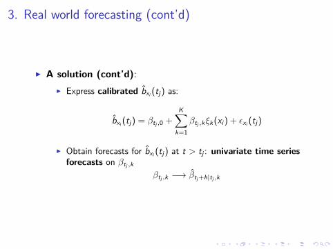
3. Real world forecasting (cont’d)

I A solution (cont’d):I Express calibrated b̂xi (tj) as:

b̂xi (tj) = βtj ,0 +K∑

k=1βtj ,kξk(xi) + εxi (tj)

I Obtain forecasts for b̂xi (tj) at t > tj : univariate time seriesforecasts on βtj ,k

βtj ,k −→ β̂tj +h|tj ,k


I A solution (cont’d):I Real world simulation: parametric law or bootstrapresampling (with replacement) of univariate time seriesresiduals

I Bootstrap:β̂tj ,k −→ β̂∗tj ,k

I Obtain univariate forecasts:

β̂∗tj +h|tj ,k

I And:b̂∗xi

(tj + h)

I Plug b̂∗xi(tj + h) into formulas for discount factors

3. Real world forecasting (cont’d)I IRS + CRA data. 12-months ahead forecasts, 1000simulations, FPCA and bootstrap resampling:


I Benchmarking with models à la Diebold-Li (2006)I Reasonable forecasts. But benchmarks are subjectiveI In practice: study the univariate time series

Model Avg. OOS error

CMN - auto.arima 0.0031CMN - ets 0.0037NS - auto.arima 0.0031NS - ets 0.0035NSS - auto.arima 0.0027NSS - ets 0.0035

I Next: use of AR(1)

3. Real world forecasting (cont’d)I IRS + CRA data. 12-months ahead forecasts, 1000simulations, FPCA and bootstrap resampling:

Questions

I Questions?

ReferencesI Ametrano, F. M., & Bianchetti, M. (2013). Everything you

always wanted to know about multiple interest rate curvebootstrapping but were afraid to ask. Available at SSRN2219548.

I Diebold, F. X., & Li, C. (2006). Forecasting the term structureof government bond yields. Journal of econometrics, 130(2),337-364.

I Hull, J., & White, A. (1990). Pricing interest-rate-derivativesecurities. Review of financial studies, 3(4), 573-592.

I Hull, J., & White, A. (1994). Branching out. Risk, 7(7), 34-37.I Ramsay, J. O., & Silverman, B. W. (2005). Springer Series in

Statistics. In Functional data analysis. Springer.I Schlögl, E., & Schlögl, L. (2000). A square root interest rate

model fitting discrete initial term structure data. AppliedMathematical Finance, 7(3), 183-209.

I Smith, A., & Wilson, T. (2001). Fitting yield curves with longterm constraints. Technical report.

presentation european actuarial journal conference 2016

Economy & Finance